Embed Size (px)
Citation preview

© A Harradine & A Lupton Draft, Oct 2008 WIP 2
Describing Change
Version 1.00 – October 2008
Written by Anthony Harradine and Alastair Lupton
Copyright © Harradine and Lupton 2008.
Copyright Information.
The materials within, in their present form, can be used free of charge for the purpose
of facilitating the learning of children in such a way that no monetary profit is made.
The materials cannot be used or reproduced in any other publications or for use in
any other way without the express permission of the authors.
© A Harradine & A Lupton Draft, Oct 2008 WIP 3
Index
Section Page
1. Managing a gas field..............................................................................5
2. Things that stack. ...................................................................................6
3. Talking about change. ...........................................................................7
4. Polygons and Angles..............................................................................9
5. Modelling Deterministic Change – 1..............................................11
6. Signal and Noise....................................................................................13
7. Modelling Stochastic Change – 1....................................................17
8. Invest smarter. ......................................................................................21
9. Simple exponential functions. ..........................................................23
10. Modelling Deterministic Change – 2..............................................24
11. Modelling Stochastic Change – 2.................................................277
12. eTech Support. .......................................................................................31
13. Answers. ................................................................................................... ??

© A Harradine & A Lupton Draft, Oct 2008 WIP 4
Using this resource.
This resource is not a text book.
It contains material that is hoped will be covered as a dialogue between students
and teacher and/or students and students.
You, as a teacher, must plan carefully ‘your performance’. The inclusion of all the
‘stuff’ is to support:
• you (the teacher) in how to plan your performance – what questions to ask,
when and so on,
• the student that may be absent,
• parents or tutors who may be unfamiliar with the way in which this approach
unfolds.
Professional development sessions in how to deliver this approach are available.
Please contact
The Noel Baker Centre for School Mathematics
Prince Alfred College,
PO Box 571 Kent Town, South Australia, 5071
Ph. +61 8 8334 1807
Email: [email protected]
Legend.
EAT – Explore And Think.
These provide an opportunity for an insight into an activity from which mathematics
will emerge – but don’t pre-empt it, just explore and think!
At certain points the learning process should have generated some
burning mathematical questions that should be discussed and pondered,
and then answered as you learn more!
Time to Formalise.
These notes document the learning that has occurred to this point,
using a degree of formal mathematical language and notation.
Examples.
Illustrations of the mathematics at hand, used to answer questions.
© A Harradine & A Lupton Draft, Oct 2008 WIP 5
1. Managing a gas field.
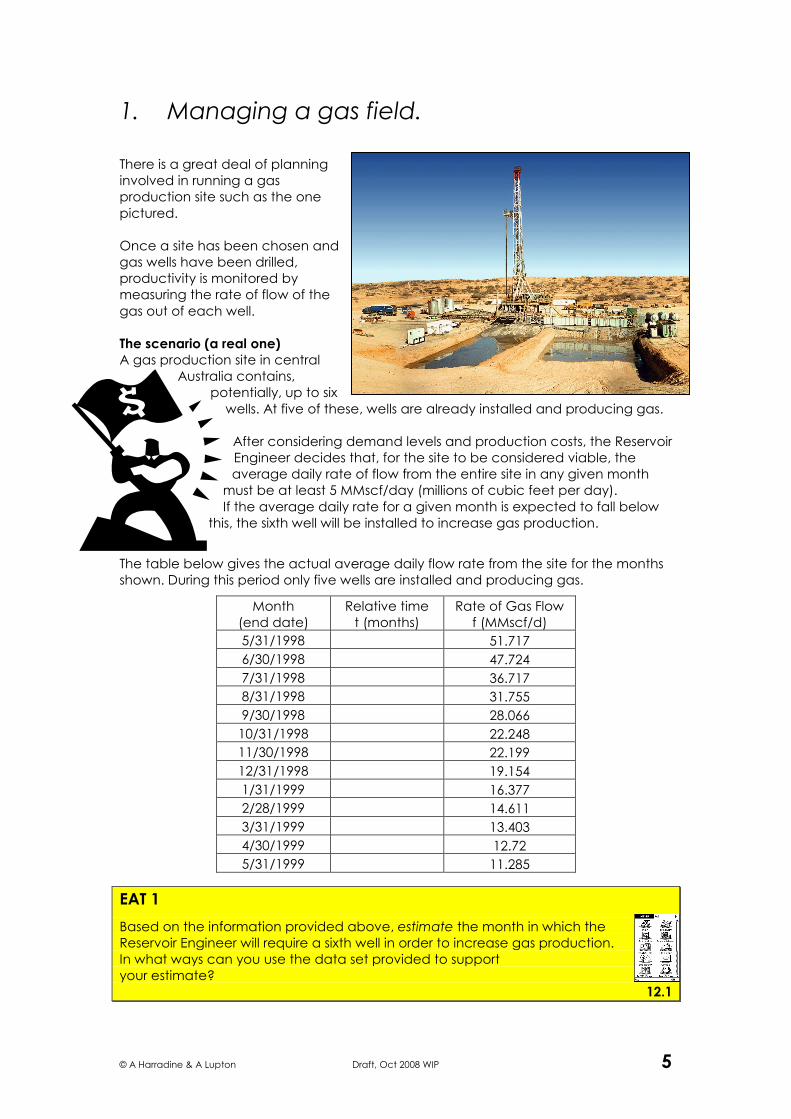
There is a great deal of planning
involved in running a gas
production site such as the one
pictured.
Once a site has been chosen and
gas wells have been drilled,
productivity is monitored by
measuring the rate of flow of the
gas out of each well.
The scenario (a real one)
A gas production site in central
Australia contains,
potentially, up to six
wells. At five of these, wells are already installed and producing gas.
After considering demand levels and production costs, the Reservoir
Engineer decides that, for the site to be considered viable, the
average daily rate of flow from the entire site in any given month
must be at least 5 MMscf/day (millions of cubic feet per day).
If the average daily rate for a given month is expected to fall below
this, the sixth well will be installed to increase gas production.
The table below gives the actual average daily flow rate from the site for the months
shown. During this period only five wells are installed and producing gas.
Month
(end date)
Relative time
t (months)
Rate of Gas Flow
f (MMscf/d)
5/31/1998 51.717
6/30/1998 47.724
7/31/1998 36.717
8/31/1998 31.755
9/30/1998 28.066
10/31/1998 22.248
11/30/1998 22.199
12/31/1998 19.154
1/31/1999 16.377
2/28/1999 14.611
3/31/1999 13.403
4/30/1999 12.72
5/31/1999 11.285
EAT 1
Based on the information provided above, estimate the month in which the
Reservoir Engineer will require a sixth well in order to increase gas production.
In what ways can you use the data set provided to support
your estimate?
12.1
© A Harradine & A Lupton Draft, Oct 2008 WIP 6
2. Things that stack.
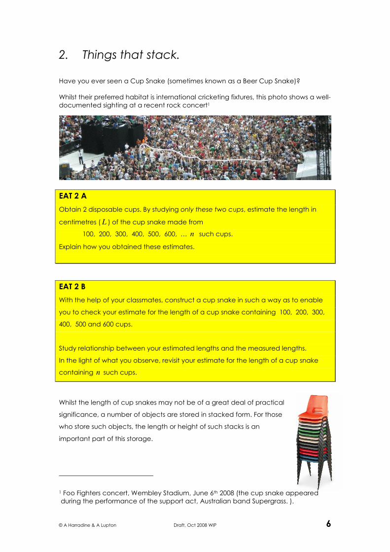
Have you ever seen a Cup Snake (sometimes known as a Beer Cup Snake)?
Whilst their preferred habitat is international cricketing fixtures, this photo shows a well-
documented sighting at a recent rock concert1
EAT 2 A
Obtain 2 disposable cups. By studying only these two cups, estimate the length in
centimetres ( L ) of the cup snake made from
100, 200, 300, 400, 500, 600, … n such cups.
Explain how you obtained these estimates.
EAT 2 B
With the help of your classmates, construct a cup snake in such a way as to enable
you to check your estimate for the length of a cup snake containing 100, 200, 300,
400, 500 and 600 cups.
Study relationship between your estimated lengths and the measured lengths.
In the light of what you observe, revisit your estimate for the length of a cup snake
containing n such cups.
Whilst the length of cup snakes may not be of a great deal of practical
significance, a number of objects are stored in stacked form. For those
who store such objects, the length or height of such stacks is an
important part of this storage.
1 Foo Fighters concert, Wembley Stadium, June 6th 2008 (the cup snake appeared
during the performance of the support act, Australian band Supergrass. ).

© A Harradine & A Lupton Draft, Oct 2008 WIP 7
3. Talking about change.
πάντα χωρεῖ καὶ οὐδὲν µένει
Change alone is unchanging
Heraclitus, 500 BC
Change can be observed in most of the systems that make up the world around us, in
simple systems like the way the balance of an investment account changes over
time, as well as in more complex systems like the growth of plants in response to
environmental factors like the supply of water and nutrients.
Human-designed systems, like the investment account, often change in regular and
predictable ways, allowing us to model these systems with a high degree of
accuracy. Change in non human-designed systems, like the growth of plants, can be
somewhat inconsistent. As a result, the modelling of such systems is harder and our
ability to predict their behaviour is more questionable.
More specifically
It is a quantity associated with a system that changes (i.e. value in $, weight in kg
etc). Hence we could say that it is the quantity that shows variation.
The variation in one quantity can often be explained by the variation in another.
Consider the following:
To what degree can
…diamond price be explained by its weight?
…the incidence of lung cancer be explained by degree of
exposure to cigarette smoke?
…global mean surface temperature be explained by the
amount of atmospheric carbon dioxide?
These questions suggest the need to explore the relationship between two quantities
or variables. We can describe this relationship in two ways.
It is likely that, in general,
• variation in diamond price is in response to variation in its weight.
• variation in the incidence of lung cancer is in response to variation in exposure
to cigarette smoke.
Or to put that another way, to some degree
• weight explains the variation in diamond price.
• exposure to cigarette smoke explains the incidence of lung cancer.
© A Harradine & A Lupton Draft, Oct 2008 WIP 8
By thinking in this way we can see that there are two different roles played by the
variables in these situations. These roles can be categorised as either
(1) Response or (2) Explanatory
In a situation, in order to determine which variable plays which role, ask yourself
Which of the variables explains the variation that occurs in the other variable?
For example, does diamond price explain the variation in weight or does
weight explain the variation in diamond price?2
In the previous three examples the following is clear,
Response Variable Explanatory Variable
Diamond Price weight
incidence of lung cancer degree of exposure to cigarette smoke
global mean surface temperature amount of atmospheric carbon dioxide
In studies, in laboratories and elsewhere, the idea is to make orderly changes to the
explanatory variable and observe the variation in the response variable.
For example, nutrient concentration can be changed in an orderly way
(i.e. increased by specific amounts) and the effect on the height of a plant can be
observed.
Sometimes, the response variable is referred to as the dependant variable, as the
value it takes tends to depend on the independent variable, with is another name for
the explanatory variable.
We have used the term explain not cause. The cause of the variation may be
something quite different to the explanatory variable.
For example, the price of a new Commodore may be explained
by time but what caused the variation?
Medical Researchers develop a new drug. They need to find the dose at which it is
most effective. The drug is developed to reduce the level of histamines in the body.
What variable are involved and what is their role?
2 More often than not the response variable is the “interesting variable” and the
explanatory variable is the “boring variable”.
© A Harradine & A Lupton Draft, Oct 2008 WIP 9
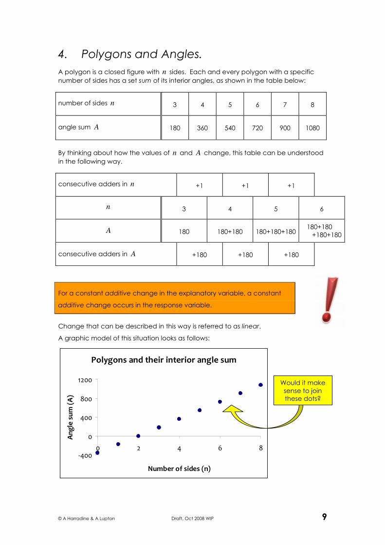
Polygons and their interior angle sum
-400
0
400
800
1200
0 2 4 6 8
Number of sides (n)
An
gle
su
m (
A)
4. Polygons and Angles.
A polygon is a closed figure with n sides. Each and every polygon with a specific
number of sides has a set sum of its interior angles, as shown in the table below:
number of sides n
3
4
5
6
7
8
angle sum A
180
360
540
720
900
1080
By thinking about how the values of n and A change, this table can be understood
in the following way.
consecutive adders in n
+1
+1
+1
n
3
4
5
6
A
180
180+180
180+180+180
180+180
+180+180
consecutive adders in A
+180
+180
+180
For a constant additive change in the explanatory variable, a constant
additive change occurs in the response variable.
Change that can be described in this way is referred to as linear.
A graphic model of this situation looks as follows:
Would it make
sense to join these dots?

© A Harradine & A Lupton Draft, Oct 2008 WIP 10
Note: A useful convention is that the explanatory variable is represented horizontally
and the response variable is represented vertically.
This system, the relationship between the interior Angle Sum ( A ) and the number of
sides ( n ) of a polygon, can be described algebraically.
Members of the family of linear functions3 cmxy += can be used to describe
systems where a constant additive change in the explanatory variable results in a
constant additive change in the response variable, as seen below
consecutive adders in x
+1
+1
1
…
1
x
0
1
2
3
…
x
y
c
cm +
cm +2
cm +3
…
cxm +
or cmx +
consecutive adders in y
m
m
m
…
m
4.1 Can you use the knowledge?
1. Write down the linear function that describes the relationship between
the interior Angle Sum ( A ) and the number of sides ( n ) of a polygon.
2. a. What is the slope / gradient of the line joining the points on the
graph of A against n on the previous page?
b. What does the slope / gradient represent in the context of system?
3. Explain the meaning of the vertical axis intercept in this context.
4. Use your linear function to determine the angle sum of a dodecagon.
5. Use your linear function to show that no polygon has an angle sum of °1680 .
6. Through geometric reasoning, it is possible deduce the relationship that we
have obtained between the interior angles and the number of sides of a
polygon. See if you can do so (a hint is provided in the Answers section).
3 A function is a mathematical rule that operates on a value (the “input” - often x ) to
obtain a unique value (the “output” - commonly y ). As such, it is a rule for obtaining
y by operating on x , sometimes referred to a rule “for y in terms of x ”.
© A Harradine & A Lupton Draft, Oct 2008 WIP 11
5. Modelling Deterministic Change – 1.
Systems, like the polygon’s internal angle sum, that change in a predictable or non-
random way are called deterministic systems. If a system’s change contains a degree
of randomness or a limited degree of predictability then it is called a stochastic
system. We are now going to work with some more deterministic systems.
5.1 Simple Interest.
In non-commercial loans (i.e. amongst family members) simple interest is often paid
by the borrower to the lender. This is a percentage of the borrowed amount, charged
per time period (i.e. per year) of the loan.
Jonathan borrows $5 400 from his father to purchase his first car. To compensate him,
Jonathan he agrees to pay him 4% p.a. (per annum or per year) in addition to the
borrowed amount (when he can afford to repay the loan).
To study the relationship between the length of the loan ( t years) and the amount
owed ($ A ) then
1. Define the role of the two variables.
2. Complete the following table
t
0
1
2
3
4
5
A
3. Explain why the relationship between these two variables is linear.
4. Represent this relationship graphically.
5. Write down the relationship between A and t algebraically.
(in other words, write down a function of A in terms of t ).
6. Use this function to determine the amount that Jonathan owes his father if
he repays the loan
a. after 10 years b. after 7 years and 9 months.
7. How long will the loan have been outstanding at the time when Jonathan
owes his father $9 000?
5.2 International Standard (SI) units – Speed.
Speed can be measured in a number of different units. Whilst in science the SI unit
metres per second is preferred, kilometres per hour is more widely understood.
Consider the following table,
© A Harradine & A Lupton Draft, Oct 2008 WIP 12
M (metres per second)
10
20
30
40
50
K (kilometres per hour)
36
72
108
144
180
1. Explain why the relationship between M and K is a linear one.
2. Write down a function for K in terms of M .
3. Use this function to convert
a. 18.6 m/s to km/h.
b. 1200 m/s to km/h.
c. 60 km/h to m/s.
d. 155 km/h to m/s.
5.3 International Standard (SI) units – Temperature.
Whilst most of the world exclusively use SI units (also known as metric units), USA and
Great Britain still frequently work with customary units (a.k.a. imperial units). When
obtaining culinary and meteorological information sourced from these countries,
temperatures are commonly given in degrees Fahrenheit. Some conversions to
degrees Celsius (the SI unit of temperature) are provided below.
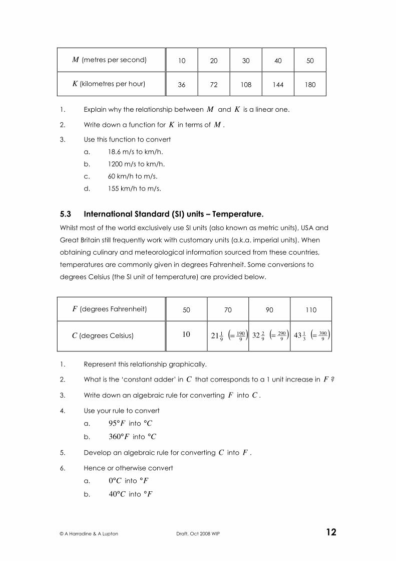
F (degrees Fahrenheit)
50
70
90
110
C (degrees Celsius)
10
( )9
1909121 =
( )9
2909232 =
( )9
3903143 =
1. Represent this relationship graphically.
2. What is the ‘constant adder’ in C that corresponds to a 1 unit increase in F ?
3. Write down an algebraic rule for converting F into C .
4. Use your rule to convert
a. F°95 into C°
b. F°360 into C°
5. Develop an algebraic rule for converting C into F .
6. Hence or otherwise convert
a. C°0 into F°
b. C°40 into F°

© A Harradine & A Lupton Draft, Oct 2008 WIP 13
6. Signal and Noise.
Recall the statement made earlier
In studies, in laboratories and elsewhere, the idea is to
make orderly changes to the explanatory variable and
observe the variation in the response variable.
It is time to look at the insights into change that can be had
when this approach is applied to a simple system like the one
pictured.
EAT 3
Set up an experiment that will allow you to gather information about the way that the
length of a helical spring (hung at one end from a fixed point as illustrated) changes
when a range of weights are suspended from the other end.
Describe the variables that will be studied in your experiment and the roles that they
play.
Predict the results of your experiment.
Conduct the experiment, record the results and compare with your predictions.

© A Harradine & A Lupton Draft, Oct 2008 WIP 14
6.1 Modelling stochastic change.
1. Complete a table similar to the following with the data that you obtained
from your experiment.
consecutive adders in m
w (weight in grams)
l (spring length in cm)
consecutive adders in l
4
For the constant additive change that you affected in the explanatory variable,
the change in the response variable was probably not exactly a constant additive
one, but sort of …
What does this suggest about a graphical representation of the
relationship between spring length and weight?
2. Represent this relationship graphically.
From your graph, two things should be clear.
• This system is not completely deterministic; there is some unpredictability
in the change that we are studying.
• The relationship between the variables is roughly linear.
As a consequence of these realisations, two more things should be apparent
• We can approximate the relationship between m and l with
a linear function.
• Such a function will represent the general trend but not the unpredictable
change, and so any use of such a model will not take into account this
behaviour.
This leaves us with two questions
• what linear function would best “fit” this relationship, and
• how to find it?
4 If you cannot complete the experiment, use the results obtained by the authors,
w (weight in grams) 0 50 100 150 200 250
l (spring length in cm) 20 20.4 22 25 27 28
© A Harradine & A Lupton Draft, Oct 2008 WIP 15
6.2 Seeking a line of best fit
1. Using your choice of electronic technology, enter your data into a
spreadsheet.
2. In two cells (e.g. D2 and E2), enter an estimate for the gradient/slope and
l -intercept of your linear model for l in terms of w .
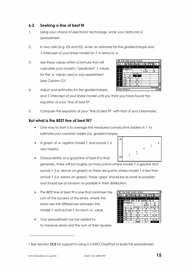
3. Use these values within a formula that will
calculate your model’s “predicted” l values
for the w values used in your experiment
(see Column C)5
4. Adjust your estimates for the gradient/slope
and l -intercept of your linear model until you think you have found the
equation of your “line of best fit”.
5. Compare the equation of your “line of best fit” with that of your classmates.
But what is the BEST line of best fit?
• One way to start is to average the measured consecutive adders in l to
estimate your constant adder (i.e. gradient/slope).
• A graph of w against model l and actual l is
very helpful.
• Characteristic of a good line of best fit is that,
generally, there will be roughly as many points where model l is greater that
actual l (i.e. above on graph) as there are points where model l is less that
actual l (i.e. below on graph). These ‘gaps’ should be as small as possible
and should be as random as possible in their distribution.
• The BEST line of best fit is one that minimises the
sum of the squares of the errors, where the
errors are the differences between the
model l and actual l for each w value.
• Your spreadsheet can be added to,
to measure errors and the sum of their squares.
5 See Section 12.2 for support in using a CASIO ClassPad to build this spreadsheet.
© A Harradine & A Lupton Draft, Oct 2008 WIP 16
0 50 100 150 200 250 300
extrapolation
interpolation
extrapolation
6.3 Using a stochastic model.
Once the line of best fit is determined and you have its equation then you can use it
to predict other values that the experiment did not reveal.
Discuss why have the word predict is used in this context.
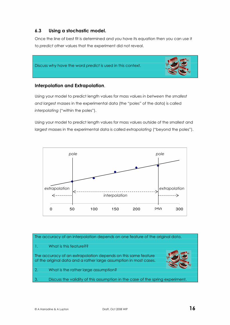
Interpolation and Extrapolation. Using your model to predict length values for mass values in between the smallest
and largest masses in the experimental data (the “poles” of the data) is called
interpolating (“within the poles”).
Using your model to predict length values for mass values outside of the smallest and
largest masses in the experimental data is called extrapolating (“beyond the poles”).
The accuracy of an interpolation depends on one feature of the original data.
1. What is this feature??
The accuracy of an extrapolation depends on this same feature
of the original data and a rather large assumption in most cases.
2. What is the rather large assumption?
3. Discuss the validity of this assumption in the case of the spring experiment.
po
pole pole

© A Harradine & A Lupton Draft, Oct 2008 WIP 17
7. Modelling Stochastic Change – 1.
12.3
7.1 Atmospheric Carbon Dioxide (CO2) over time – part 1.
For many years the concentration of Carbon Dioxide in the atmosphere
(measured in p.p.m. – parts per million) has been recorded at Mauna Loa, Hawaii.
The most recent 8 years of data from Mauna Loa are recorded below.
Year 2000 2001 2002 2003 2004 2005 2006 2007
Atmospheric concentration
of Carbon Dioxide (p.p.m.) 369.48 371.02 373.1 375.64 377.38 380.99 382.71 384.5
1. Represent this data graphically.
2. By considering the average additive change in C , the quantity of
atmospheric CO2 in p.p.m., over successive years, write down a linear model for C in terms of t , the number of years since 2000.
3. Sketch your model from part 2 on your graph from part 1.
4. Refine, if necessary, the co-efficients of your linear model in the light on this
sketch.
5. Use your linear model to predict the concentration of Carbon Dioxide in the
atmosphere in the year 2010.
6. Scientist warn of the potential significant climate change if the
concentration of Carbon Dioxide in the atmosphere exceeds 400 p.p.m.
According to your model, in what year will that quantity be exceeded?
7. What assumption are you making in your answering on part 6?
7.2 A stochastic process.
A stochastic process has generated the following data:
x 5 10 15 20 25 30 35 40 45 50 y 997 932 893 825 837 797 727 646 605 611
1. Draw a scatter plot of this data.
2. Calculate the average additive change in y for a one-unit increase in x , and
hence develop a linear model for y in terms of x .
3. Sketch your model from part 2 on your graph from part 1.
4. Refine, if necessary, the co-efficients of your linear model in the light on this
sketch.
5. Use your linear model to predict the result of this stochastic process if x = 65.
© A Harradine & A Lupton Draft, Oct 2008 WIP 18
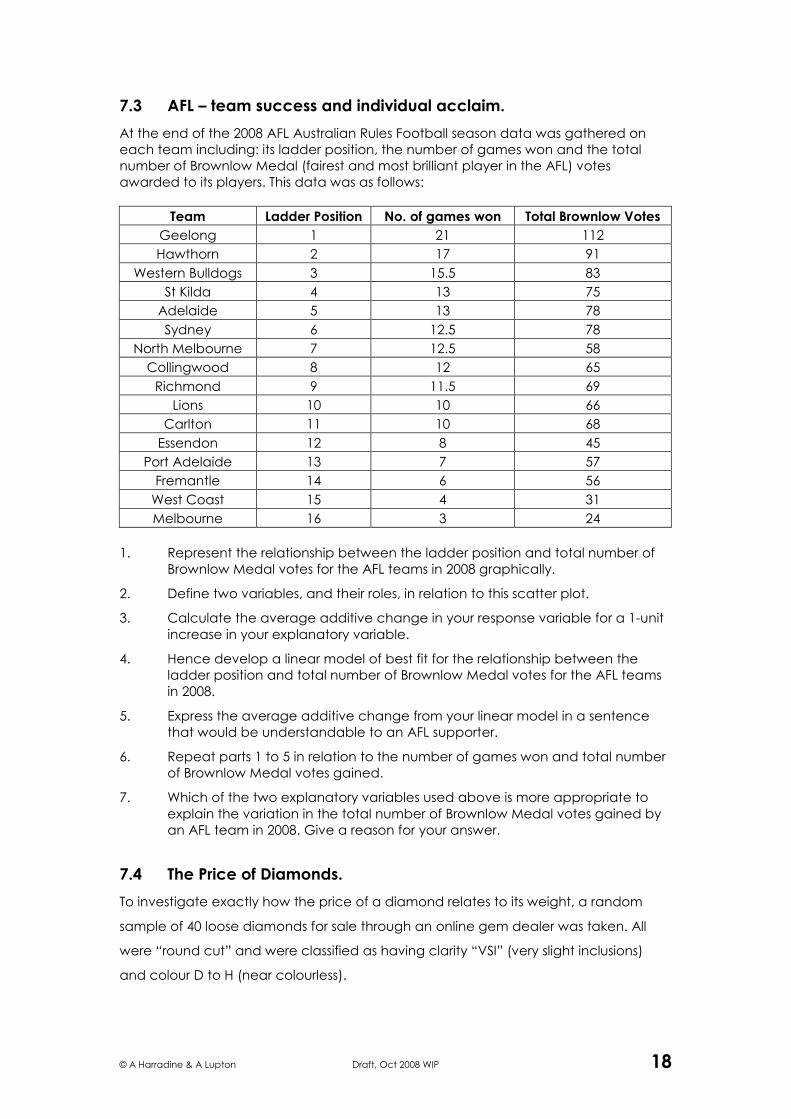
7.3 AFL – team success and individual acclaim.
At the end of the 2008 AFL Australian Rules Football season data was gathered on
each team including: its ladder position, the number of games won and the total
number of Brownlow Medal (fairest and most brilliant player in the AFL) votes
awarded to its players. This data was as follows:
Team Ladder Position No. of games won Total Brownlow Votes
Geelong 1 21 112
Hawthorn 2 17 91
Western Bulldogs 3 15.5 83
St Kilda 4 13 75
Adelaide 5 13 78
Sydney 6 12.5 78
North Melbourne 7 12.5 58
Collingwood 8 12 65
Richmond 9 11.5 69
Lions 10 10 66
Carlton 11 10 68
Essendon 12 8 45
Port Adelaide 13 7 57
Fremantle 14 6 56
West Coast 15 4 31
Melbourne 16 3 24
1. Represent the relationship between the ladder position and total number of
Brownlow Medal votes for the AFL teams in 2008 graphically.
2. Define two variables, and their roles, in relation to this scatter plot.
3. Calculate the average additive change in your response variable for a 1-unit
increase in your explanatory variable.
4. Hence develop a linear model of best fit for the relationship between the
ladder position and total number of Brownlow Medal votes for the AFL teams
in 2008.
5. Express the average additive change from your linear model in a sentence
that would be understandable to an AFL supporter.
6. Repeat parts 1 to 5 in relation to the number of games won and total number
of Brownlow Medal votes gained.
7. Which of the two explanatory variables used above is more appropriate to
explain the variation in the total number of Brownlow Medal votes gained by
an AFL team in 2008. Give a reason for your answer.
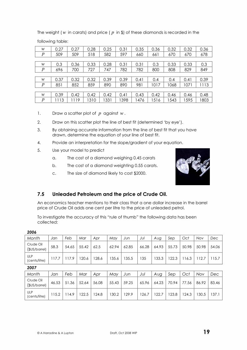
7.4 The Price of Diamonds.
To investigate exactly how the price of a diamond relates to its weight, a random
sample of 40 loose diamonds for sale through an online gem dealer was taken. All
were “round cut” and were classified as having clarity “VSI” (very slight inclusions)
and colour D to H (near colourless).
© A Harradine & A Lupton Draft, Oct 2008 WIP 19
The weight ( w in carats) and price ( p in $) of these diamonds is recorded in the
following table:
w 0.27 0.27 0.28 0.25 0.31 0.35 0.36 0.32 0.32 0.36 p 509 509 518 582 597 660 661 670 670 678
w 0.3 0.36 0.33 0.28 0.31 0.31 0.3 0.33 0.33 0.3 p 696 700 727 747 782 782 800 808 829 849
w 0.37 0.32 0.32 0.39 0.39 0.41 0.4 0.4 0.41 0.39 p 851 852 859 890 890 981 1017 1068 1071 1113
w 0.39 0.42 0.42 0.42 0.41 0.43 0.42 0.46 0.46 0.48 p 1113 1119 1310 1331 1398 1476 1516 1543 1595 1803
1. Draw a scatter plot of p against w .
2. Draw on this scatter plot the line of best fit (determined ‘by eye’).
3. By obtaining accurate information from the line of best fit that you have
drawn, determine the equation of your line of best fit.
4. Provide an interpretation for the slope/gradient of your equation.
5. Use your model to predict
a. The cost of a diamond weighing 0.45 carats
b. The cost of a diamond weighting 0.55 carats.
c. The size of diamond likely to cost $2000.
7.5 Unleaded Petroleum and the price of Crude Oil.
An economics teacher mentions to their class that a one dollar increase in the barrel
price of Crude Oil adds one cent per litre to the price of unleaded petrol.
To investigate the accuracy of this “rule of thumb” the following data has been
collected:
2006
Month Jan Feb Mar Apr May Jun Jul Aug Sep Oct Nov Dec
Crude Oil ($US/barrel)
58.3 54.65 55.42 62.5 62.94 62.85 66.28 64.93 55.73 50.98 50.98 54.06
ULP
(cents/litre) 117.7 117.9 120.6 128.6 135.6 135.5 135 133.3 122.3 116.3 112.7 115.7
2007
Month Jan Feb Mar Apr May Jun Jul Aug Sep Oct Nov Dec
Crude Oil ($US/barrel)
46.53 51.36 52.64 56.08 55.43 59.25 65.96 64.23 70.94 77.56 86.92 83.46
ULP (cents/litre)
115.2 114.9 122.5 124.8 130.2 129.9 126.7 122.7 123.8 124.3 130.5 137.1

© A Harradine & A Lupton Draft, Oct 2008 WIP 20
1. Define the variables and their roles in this situation.
2. Develop a model that best fits this data.
3. With reference to your model, comment on the “rule of thumb” quoted
above. If necessary, formulate a revised rule of thumb.
4. Use your model to predict
a. The price of ULP if crude oil cost $80 per barrel.
b. The level to which the cost of crude oil will have risen if the
cost of ULP reaches $8.00 per litre
(CSIRO worst case scenario for 2018).
12.4
2008
Month Jan Feb Mar Apr May Jun
Crude Oil ($US/barrel)
84.7 86.64 96.87 104.31 117.4 126.33
ULP
(cents/litre) 138.6 136.1 139.7 143.1 148.9 157.8

© A Harradine & A Lupton Draft, Oct 2008 WIP 21
8. Invest smarter.
Compound Interest … explains why $1000 … can grow to $47 000
over 50 years. No wonder Albert Einstein described compound interest
as one of the greatest human discoveries
ipac finacial services
EAT 4 How does Compound Interest work?
Consider an investment of $1 000 that earns 6% interest p.a.
In the 1st year, how much interest is earned?
Therefore, what is the total value of the investment after the 1st year?
Based on this,
In the 2nd year, how much interest is earned?
Therefore, what is the value of the investment after the 2nd year?
Repeat this for the 3rd, 4th and 5th years.
Can you write down a model for V , the value of the investment after n years?
Is this a deterministic or stochastic model? Why?
If you can write down a model for V in terms of n , use it to predict the value of
the investment after 50 years.
If this value is not $47 000, how would the scenario have to changed if the
claim above was to be accurate?
What different ways were used to perform the
calculations required in EAT 4?
Which way was easiest?
How do you (easily) increase an amount by 15%? 80%? 1%?
© A Harradine & A Lupton Draft, Oct 2008 WIP 22
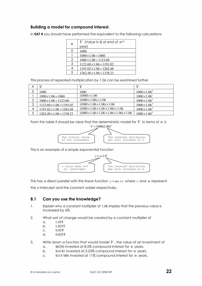
Building a model for compound interest.
In EAT 4 you should have performed the equivalent to the following calculations
n V (Value in $ at end of n th
year)
0 1000 1 1000 ×1.06 = 1060 2 1060 ×1.06 = 1123.60 3 1123.60 ×1.06 = 1191.02 4 1191.02 ×1.06 = 1262.48 5 1262.48 ×1.06 = 1338.23
This process of repeated multiplication by 1.06 can be examined further
n V V V
0 1000 1000 1000 ×1.060 1 1000 ×1.06 = 1060 (1000) ×1.06 1000 ×1.061 2 1060 ×1.06 = 1123.60 (1000 ×1.06) ×1.06 1000 ×1.062 3 1123.60 ×1.06 = 1191.02 (1000 ×1.06 ×1.06) ×1.06 1000 ×1.063 4 1191.02 ×1.06 = 1262.48 (1000 ×1.06 ×1.06 ×1.06) ×1.06 1000 ×1.064 5 1262.48 ×1.06 = 1338.23 (1000 ×1.06 ×1.06 ×1.06 ×1.06) ×1.06 1000 ×1.065
From this table it should be clear that the deterministic model for V in terms of n is
V = 1000(1.06)n
This is an example of a simple exponential function
y = a × bx
This has a direct parallel with the linear function y = mx + c where c and m represent
the y-intercept and the constant adder respectively.
8.1 Can you use the knowledge?
1. Explain why a constant multiplier of 1.06 implies that the previous value is
increased by 6%.
2. What sort of change would be created by a constant multiplier of
a. 1.45?
b. 1.025?
c. 0.95?
d. 0.825?
3. Write down a function that would model V , the value of an investment of
a. $6250 invested at 8.5% compound interest for n years.
b. $14.92 invested at 2.25% compound interest for n years.
c. $115 000 invested at 11% compound interest for n years.
The initial value of the investment
The constant multiplier per unit increase in n
y value when x=0 (y- intercept)
The constant multiplier per unit increase in x
© A Harradine & A Lupton Draft, Oct 2008 WIP 23
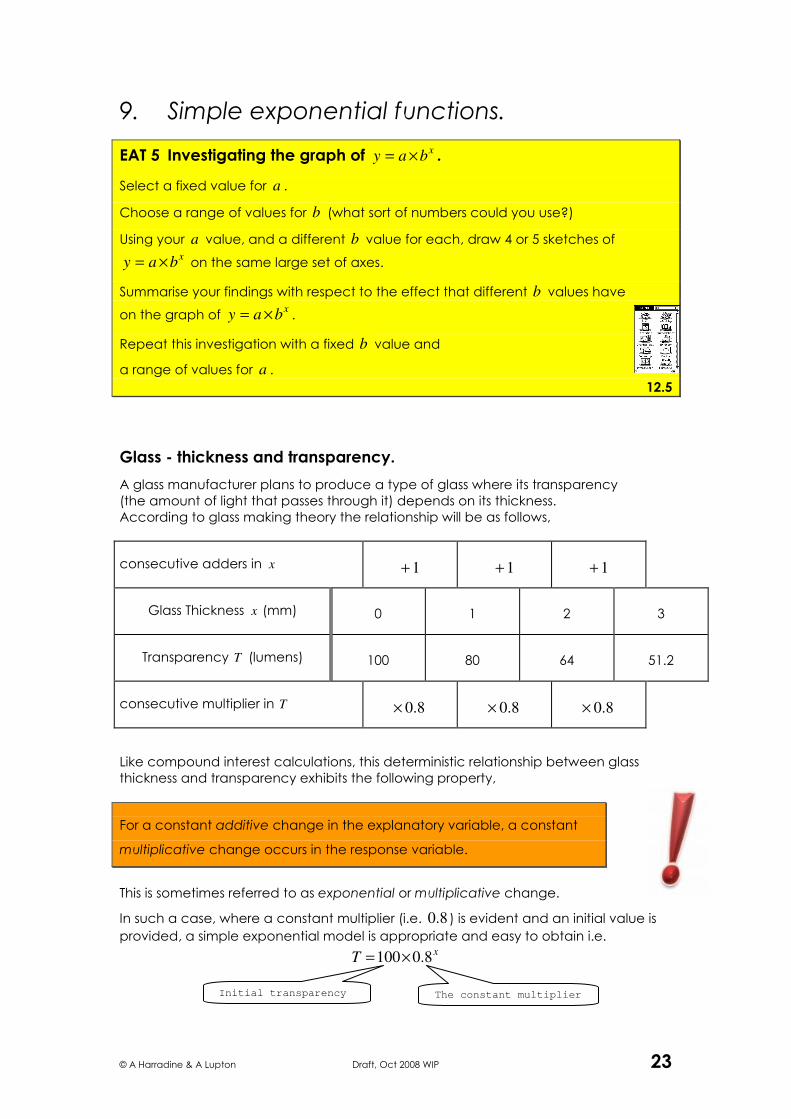
9. Simple exponential functions.
EAT 5 Investigating the graph of xbay ×= .
Select a fixed value for a .
Choose a range of values for b (what sort of numbers could you use?)
Using your a value, and a different b value for each, draw 4 or 5 sketches of x
bay ×= on the same large set of axes.
Summarise your findings with respect to the effect that different b values have
on the graph of x
bay ×= .
Repeat this investigation with a fixed b value and
a range of values for a .
12.5
Glass - thickness and transparency.
A glass manufacturer plans to produce a type of glass where its transparency
(the amount of light that passes through it) depends on its thickness.
According to glass making theory the relationship will be as follows,
consecutive adders in x
1+
1+
1+
Glass Thickness x (mm)
0
1
2
3
Transparency T (lumens)
100
80
64
51.2
consecutive multiplier in T
8.0×
8.0×
8.0×
Like compound interest calculations, this deterministic relationship between glass
thickness and transparency exhibits the following property,
For a constant additive change in the explanatory variable, a constant
multiplicative change occurs in the response variable.
This is sometimes referred to as exponential or multiplicative change.
In such a case, where a constant multiplier (i.e. 8.0 ) is evident and an initial value is
provided, a simple exponential model is appropriate and easy to obtain i.e. x
T 8.0100×=
Initial transparency The constant multiplier
© A Harradine & A Lupton Draft, Oct 2008 WIP 24
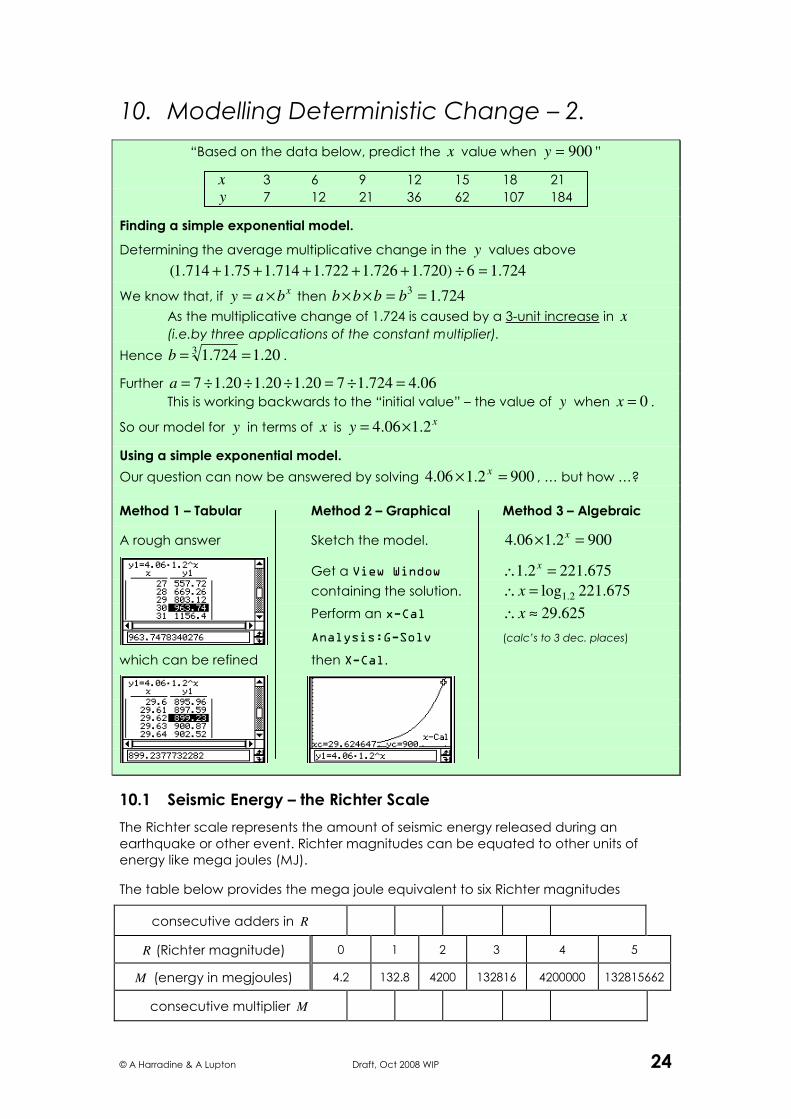
10. Modelling Deterministic Change – 2.
“Based on the data below, predict the x value when 900=y ”
x 3 6 9 12 15 18 21
y 7 12 21 36 62 107 184
Finding a simple exponential model.
Determining the average multiplicative change in the y values above
724.16)720.1726.1722.1714.175.1714.1( =÷+++++
We know that, if xbay ×= then 724.13
==×× bbbb
As the multiplicative change of 1.724 is caused by a 3-unit increase in x
(i.e.by three applications of the constant multiplier).
Hence 20.1724.13 ==b .
Further 06.4724.1720.120.120.17 =÷=÷÷÷=a
This is working backwards to the “initial value” – the value of y when 0=x .
So our model for y in terms of x is xy 2.106.4 ×=
Using a simple exponential model.
Our question can now be answered by solving 9002.106.4 =×x
, … but how …?
Method 1 – Tabular Method 2 – Graphical Method 3 – Algebraic
A rough answer Sketch the model. 9002.106.4 =×x
Get a View Window 675.2212.1 =∴x
containing the solution. 675.221log 2.1=∴ x
Perform an x-Cal 625.29≈∴ x
Analysis:G-Solv (calc’s to 3 dec. places)
which can be refined then X-Cal.
10.1 Seismic Energy – the Richter Scale
The Richter scale represents the amount of seismic energy released during an
earthquake or other event. Richter magnitudes can be equated to other units of
energy like mega joules (MJ).
The table below provides the mega joule equivalent to six Richter magnitudes
consecutive adders in R
R (Richter magnitude) 0 1 2 3 4 5
M (energy in megjoules) 4.2 132.8 4200 132816 4200000 132815662
consecutive multiplier M

© A Harradine & A Lupton Draft, Oct 2008 WIP 25
1. Using the previous table, write down a model for M in terms of R .
2. Use this model to determine the energy released (in MJ) by the earthquake
that devastated Kashmir in 2005 which measured 7.5 on the Richter Scale.
3. The Valdivia Earthquake that struck Chile in 1960 measured 9.5 on the Richter
Scale, one of the highest ever recorded.
How many MJ of energy did it release?
4. Describe the difference in energy release between earthquakes that
differ by two on the Richter scale.
10.2 Depreciation.
According to a company’s Depreciation Schedule, an assets “book value” in the
years after purchase is as follows;
t (years since purchase) 0 1 2 3 4 5
V (book value – whole $’s) 112500 95625 81281 69089 58725 49916
1. Interpret the constant multiplier evident in the relationship between V and t .
2. Write down a simple exponential model for this relationship.
3. Hence determine the book value of the asset
a. 10 years after purchase.
b. 13.5 years after purchase.
4. In what year does the book value of the asset fall below $5000?
10.3 Radioactive Decay.
The radioactive isotope Thorium 234 decays (by beta-emission of radioactivity into
protactinium-234) in the following way
t (days) 0 4 8 12 16 20
W (mass of remaining
Thorium-234 in grams) 100 89 79.4 70.7 63 56.1
1. Determine the constant multiplier in W for a one-unit increase in t .
Interpret this value in the context of the question.
2. Write down a simple exponential model for this relationship.
3. Hence the amount of Thorium-234 remaining after
a. 7 days.
b. 365 days.
4. What is the half-life of Thorium-234?
(An isotope’s half-life is the time taken for it to decay to half its mass)
© A Harradine & A Lupton Draft, Oct 2008 WIP 26
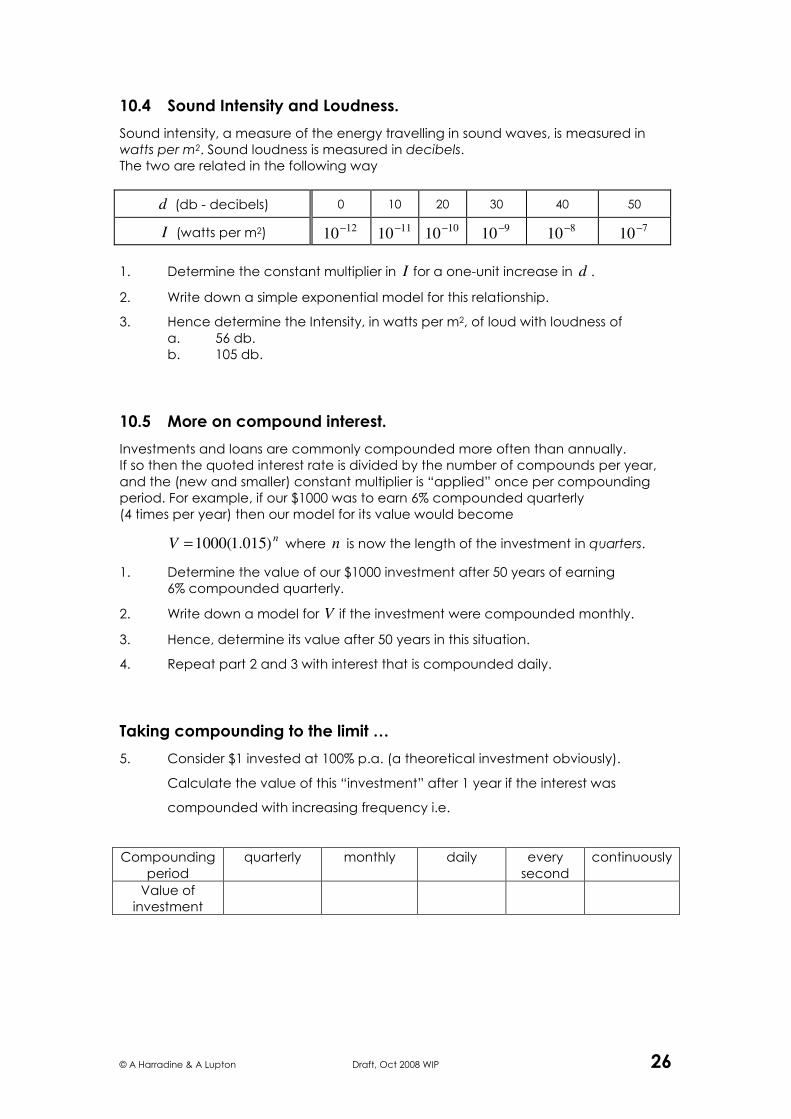
10.4 Sound Intensity and Loudness.
Sound intensity, a measure of the energy travelling in sound waves, is measured in
watts per m2. Sound loudness is measured in decibels.
The two are related in the following way
d (db - decibels) 0 10 20 30 40 50
I (watts per m2) 1210−
1110−
1010−
910−
810−
710−
1. Determine the constant multiplier in I for a one-unit increase in d .
2. Write down a simple exponential model for this relationship.
3. Hence determine the Intensity, in watts per m2, of loud with loudness of
a. 56 db.
b. 105 db.
10.5 More on compound interest.
Investments and loans are commonly compounded more often than annually.
If so then the quoted interest rate is divided by the number of compounds per year,
and the (new and smaller) constant multiplier is “applied” once per compounding
period. For example, if our $1000 was to earn 6% compounded quarterly
(4 times per year) then our model for its value would become
nV )015.1(1000= where n is now the length of the investment in quarters.
1. Determine the value of our $1000 investment after 50 years of earning
6% compounded quarterly.
2. Write down a model for V if the investment were compounded monthly.
3. Hence, determine its value after 50 years in this situation.
4. Repeat part 2 and 3 with interest that is compounded daily.
Taking compounding to the limit …
5. Consider $1 invested at 100% p.a. (a theoretical investment obviously).
Calculate the value of this “investment” after 1 year if the interest was
compounded with increasing frequency i.e.
Compounding
period
quarterly monthly daily every
second
continuously
Value of
investment
© A Harradine & A Lupton Draft, Oct 2008 WIP 27
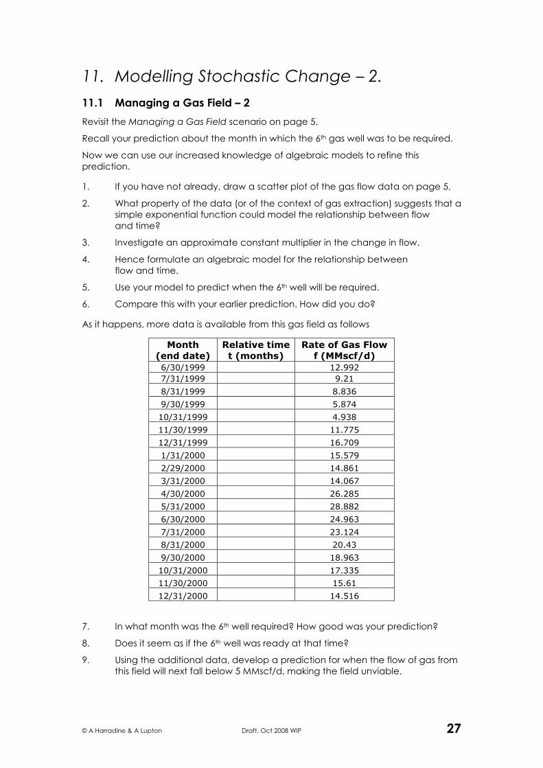
11. Modelling Stochastic Change – 2.
11.1 Managing a Gas Field – 2
Revisit the Managing a Gas Field scenario on page 5.
Recall your prediction about the month in which the 6th gas well was to be required.
Now we can use our increased knowledge of algebraic models to refine this
prediction.
1. If you have not already, draw a scatter plot of the gas flow data on page 5.
2. What property of the data (or of the context of gas extraction) suggests that a
simple exponential function could model the relationship between flow
and time?
3. Investigate an approximate constant multiplier in the change in flow.
4. Hence formulate an algebraic model for the relationship between
flow and time.
5. Use your model to predict when the 6th well will be required.
6. Compare this with your earlier prediction. How did you do?
As it happens, more data is available from this gas field as follows
7. In what month was the 6th well required? How good was your prediction?
8. Does it seem as if the 6th well was ready at that time?
9. Using the additional data, develop a prediction for when the flow of gas from
this field will next fall below 5 MMscf/d, making the field unviable.
Month
(end date)
Relative time
t (months)
Rate of Gas Flow
f (MMscf/d)
6/30/1999 12.992
7/31/1999 9.21
8/31/1999 8.836
9/30/1999 5.874
10/31/1999 4.938
11/30/1999 11.775
12/31/1999 16.709
1/31/2000 15.579
2/29/2000 14.861
3/31/2000 14.067
4/30/2000 26.285
5/31/2000 28.882
6/30/2000 24.963
7/31/2000 23.124
8/31/2000 20.43
9/30/2000 18.963
10/31/2000 17.335
11/30/2000 15.61
12/31/2000 14.516
© A Harradine & A Lupton Draft, Oct 2008 WIP 28
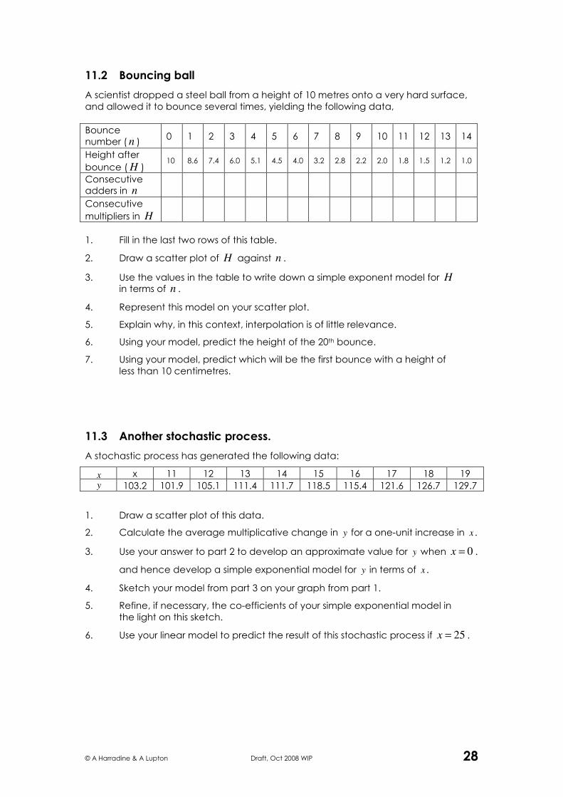
11.2 Bouncing ball
A scientist dropped a steel ball from a height of 10 metres onto a very hard surface,
and allowed it to bounce several times, yielding the following data,
Bounce number ( n )
0 1 2 3 4 5 6 7 8 9 10 11 12 13 14
Height after
bounce ( H ) 10 8.6 7.4 6.0 5.1 4.5 4.0 3.2 2.8 2.2 2.0 1.8 1.5 1.2 1.0
Consecutive adders in n
Consecutive
multipliers in H
1. Fill in the last two rows of this table.
2. Draw a scatter plot of H against n .
3. Use the values in the table to write down a simple exponent model for H in terms of n .
4. Represent this model on your scatter plot.
5. Explain why, in this context, interpolation is of little relevance.
6. Using your model, predict the height of the 20th bounce.
7. Using your model, predict which will be the first bounce with a height of
less than 10 centimetres.
11.3 Another stochastic process.
A stochastic process has generated the following data:
x x 11 12 13 14 15 16 17 18 19 y 103.2 101.9 105.1 111.4 111.7 118.5 115.4 121.6 126.7 129.7
1. Draw a scatter plot of this data.
2. Calculate the average multiplicative change in y for a one-unit increase in x .
3. Use your answer to part 2 to develop an approximate value for y when 0=x .
and hence develop a simple exponential model for y in terms of x .
4. Sketch your model from part 3 on your graph from part 1.
5. Refine, if necessary, the co-efficients of your simple exponential model in
the light on this sketch.
6. Use your linear model to predict the result of this stochastic process if 25=x .

© A Harradine & A Lupton Draft, Oct 2008 WIP 29
11.4 Worldwide use of the WWW.
According to an internet monitor, the percentage of the world’s population that uses
the internet (at least monthly) has changed, since 1995, in the following way:
years
since ‘95 0 1 2 3 4 5 6 7 8 9 10 11 12
WWW
use (%) 0.4 0.9 1.7 3.6 4.1 5.8 8.6 9.4 11.1 12.7 15.7 16.7 20
1. Represent this data on a scatter plot.
2. Explain why a linear model is not able to capture the change in use of the
world wide web since 1995.
3. Investigate the possibility of modelling this change with a simple exponential
model.
4. Use technology to obtain a quadratic model of best fit for this data.
5. Use your preferred model from parts 3 or 4 to predict when a third of the world
will use the internet (at least monthly).
6. How accurate do you think the prediction asked for in part 5 is likely to be?
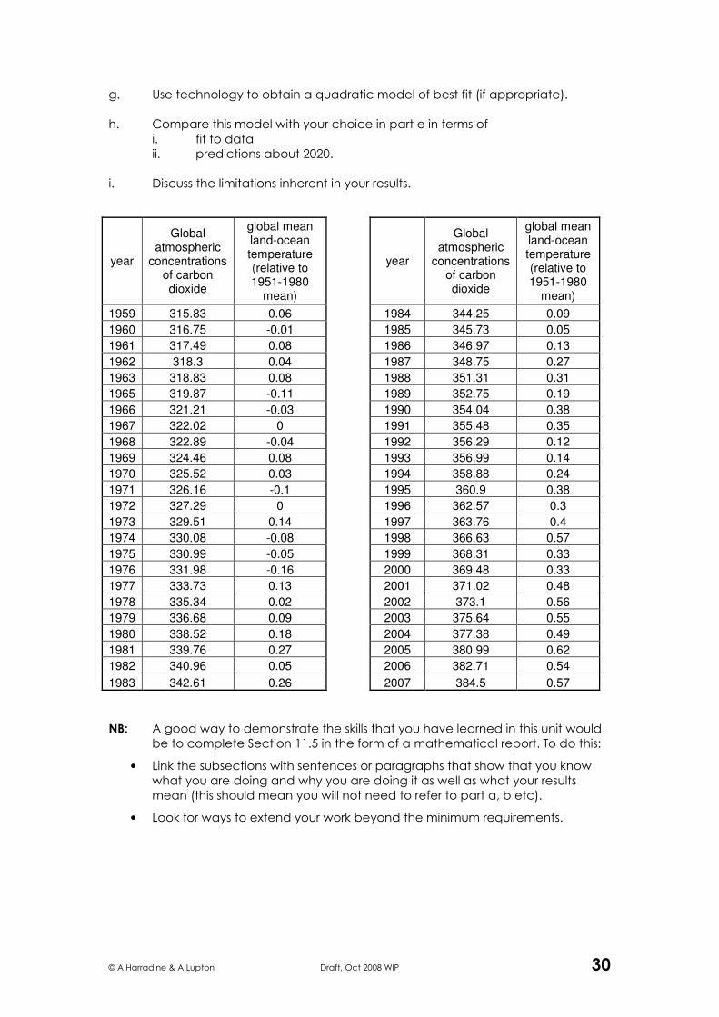
11.5 Global Temperature and Atmospheric CO2.
The table provided contains the annual data from Mauna Loa, the longest running
atmospheric monitoring station based in Hawaii, along with the global mean land-
ocean temperature (relative to the 1951-1980 mean) for the years after 1959.
Investigate appropriate models for
1. atmospheric CO2 in terms of years since 1959,
2. global mean land-ocean temperature in terms of years since 1959
3. global mean land-ocean temperature in terms of atmospheric CO2.
In each case,
a. Assign variables and classify their role.
b. Determine the type of algebraic model that you will use to describe the
relationship between the variables, explaining the reasons for your selection.
c. Determine the equation of the line / curve of best fit, using the concepts of
“constant adder / multiplier” and a “graph and refine” method, with
documentation.
d. Use the model fitting capacity of your choice of technology to find the
equation of an alternative line / curve of best fit.
e. Compare the models obtained in parts c and d and select your choice of
model. Give reasons for your selection.
f. Use your choice of model to make predictions about 2020.
© A Harradine & A Lupton Draft, Oct 2008 WIP 30
g. Use technology to obtain a quadratic model of best fit (if appropriate).
h. Compare this model with your choice in part e in terms of
i. fit to data
ii. predictions about 2020.
i. Discuss the limitations inherent in your results.
NB: A good way to demonstrate the skills that you have learned in this unit would
be to complete Section 11.5 in the form of a mathematical report. To do this:
• Link the subsections with sentences or paragraphs that show that you know
what you are doing and why you are doing it as well as what your results
mean (this should mean you will not need to refer to part a, b etc).
• Look for ways to extend your work beyond the minimum requirements.
year
Global atmospheric
concentrations of carbon dioxide
global mean land-ocean temperature (relative to 1951-1980
mean)
year
Global atmospheric
concentrations of carbon dioxide
global mean land-ocean temperature (relative to 1951-1980
mean)
1959 315.83 0.06 1984 344.25 0.09
1960 316.75 -0.01 1985 345.73 0.05
1961 317.49 0.08 1986 346.97 0.13
1962 318.3 0.04 1987 348.75 0.27
1963 318.83 0.08 1988 351.31 0.31
1965 319.87 -0.11 1989 352.75 0.19
1966 321.21 -0.03 1990 354.04 0.38
1967 322.02 0 1991 355.48 0.35
1968 322.89 -0.04 1992 356.29 0.12
1969 324.46 0.08 1993 356.99 0.14
1970 325.52 0.03 1994 358.88 0.24
1971 326.16 -0.1 1995 360.9 0.38
1972 327.29 0 1996 362.57 0.3
1973 329.51 0.14 1997 363.76 0.4
1974 330.08 -0.08 1998 366.63 0.57
1975 330.99 -0.05 1999 368.31 0.33
1976 331.98 -0.16 2000 369.48 0.33
1977 333.73 0.13 2001 371.02 0.48
1978 335.34 0.02 2002 373.1 0.56
1979 336.68 0.09 2003 375.64 0.55
1980 338.52 0.18 2004 377.38 0.49
1981 339.76 0.27 2005 380.99 0.62
1982 340.96 0.05 2006 382.71 0.54
1983 342.61 0.26 2007 384.5 0.57
© A Harradine & A Lupton Draft, Oct 2008 WIP 31
12. eTech Support.
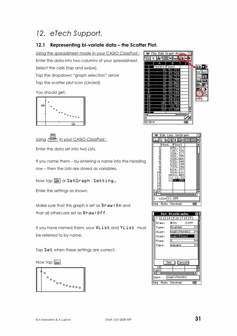
12.1 Representing bi-variate data – the Scatter Plot.
Using the spreadsheet mode in your CASIO ClassPad :
Enter the data into two columns of your spreadsheet.
Select the cells (tap and swipe).
Tap the dropdown “graph selection” arrow
Tap the scatter plot icon (circled)
You should get:
Using I in your CASIO ClassPad :
Enter the data set into two Lists.
If you name them – by entering a name into the heading
row – then the Lists are stored as variables.
Now tap G or SetGraph : Setting…
Enter the settings as shown.
Make sure that this graph is set as Draw:On and
that all others are set as Draw:Off.
If you have named them, your XList and YList must
be referred to by name.
Tap Set when these settings are correct.
Now tap y
© A Harradine & A Lupton Draft, Oct 2008 WIP 32
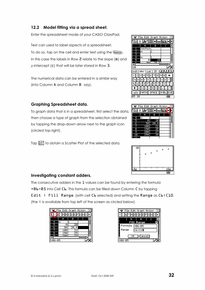
12.2 Model fitting via a spread sheet.
Enter the spreadsheet mode of your CASIO ClassPad.
Text can used to label aspects of a spreadsheet.
To do so, tap on the cell and enter text using the k.
In this case the labels in Row 2 relate to the slope (m) and
y-intercept (c) that will be later stored in Row 3.
The numerical data can be entered in a similar way
(into Column A and Column B say).
Graphing Spreadsheet data.
To graph data that is in a spreadsheet, first select the data,
then choose a type of graph from the selection obtained
by tapping the drop-down arrow next to the graph icon
(circled top right).
Tap X to obtain a Scatter Plot of the selected data.
Investigating constant adders.
The consecutive adders in the l-values can be found by entering the formula
=B6-B5 into Cell C6. This formula can be filled down Column C by tapping
Edit : Fill Range. (with cell C6 selected) and setting the Range as C6:C10.
(the : is available from top left of the screen as circled below)
© A Harradine & A Lupton Draft, Oct 2008 WIP 33
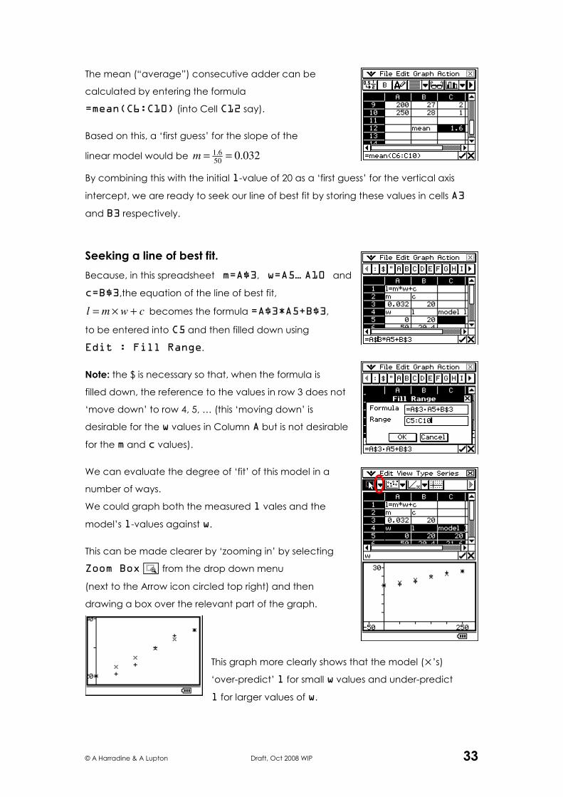
The mean (“average”) consecutive adder can be
calculated by entering the formula
=mean(C6:C10) (into Cell C12 say).
Based on this, a ‘first guess’ for the slope of the
linear model would be 032.050
6.1 ==m
By combining this with the initial l-value of 20 as a ‘first guess’ for the vertical axis
intercept, we are ready to seek our line of best fit by storing these values in cells A3
and B3 respectively.
Seeking a line of best fit.
Because, in this spreadsheet m=A$3, w=A5… A10 and
c=B$3,the equation of the line of best fit,
cwml +×= becomes the formula =A$3*A5+B$3,
to be entered into C5 and then filled down using
Edit : Fill Range.
Note: the $ is necessary so that, when the formula is
filled down, the reference to the values in row 3 does not
‘move down’ to row 4, 5, … (this ‘moving down’ is
desirable for the w values in Column A but is not desirable
for the m and c values).
We can evaluate the degree of ‘fit’ of this model in a
number of ways.
We could graph both the measured l vales and the
model’s l-values against w.
This can be made clearer by ‘zooming in’ by selecting
Zoom Box Q from the drop down menu
(next to the Arrow icon circled top right) and then
drawing a box over the relevant part of the graph.
This graph more clearly shows that the model (× ’s)
‘over-predict’ l for small w values and under-predict
l for larger values of w.
© A Harradine & A Lupton Draft, Oct 2008 WIP 34
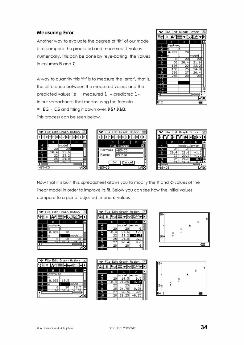
Measuring Error
Another way to evaluate the degree of ‘fit’ of our model
is to compare the predicted and measured l-values
numerically. This can be done by ‘eye-balling’ the values
in columns B and C.
A way to quantity this ‘fit’ is to measure the ‘error’, that is,
the difference between the measured values and the
predicted values i.e measured l – predicted l.
In our spreadsheet that means using the formula
= B5 – C5 and filling it down over D5:D10.
This process can be seen below.
Now that it is built this, spreadsheet allows you to modify the m and c-values of the
linear model in order to improve its fit. Below you can see how the initial values
compare to a pair of adjusted m and c-values
© A Harradine & A Lupton Draft, Oct 2008 WIP 35
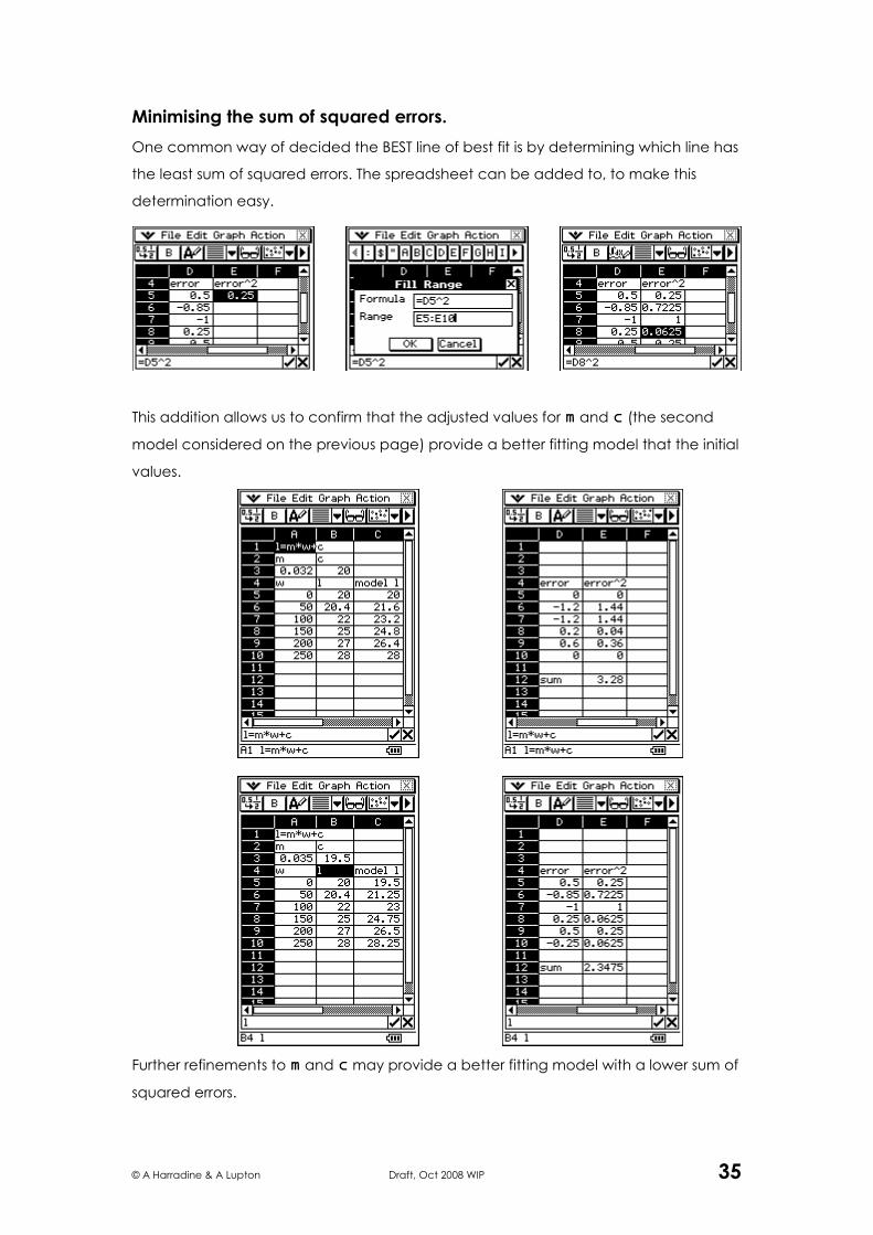
Minimising the sum of squared errors.
One common way of decided the BEST line of best fit is by determining which line has
the least sum of squared errors. The spreadsheet can be added to, to make this
determination easy.
This addition allows us to confirm that the adjusted values for m and c (the second
model considered on the previous page) provide a better fitting model that the initial
values.
Further refinements to m and c may provide a better fitting model with a lower sum of
squared errors.
© A Harradine & A Lupton Draft, Oct 2008 WIP 36
12.3 Working with data and models.
Calculating Additive Change
See Section 12.2. on the use of the ClassPad’s spreadsheet.
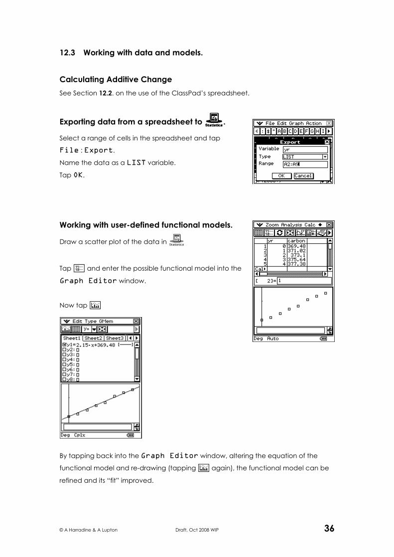
Exporting data from a spreadsheet to IIII.
Select a range of cells in the spreadsheet and tap
File : Export.
Name the data as a LIST variable.
Tap OK.
Working with user-defined functional models.
Draw a scatter plot of the data in I
Tap ! and enter the possible functional model into the
Graph Editor window.
Now tap y
By tapping back into the Graph Editor window, altering the equation of the
functional model and re-drawing (tapping y again), the functional model can be
refined and its “fit” improved.
© A Harradine & A Lupton Draft, Oct 2008 WIP 37
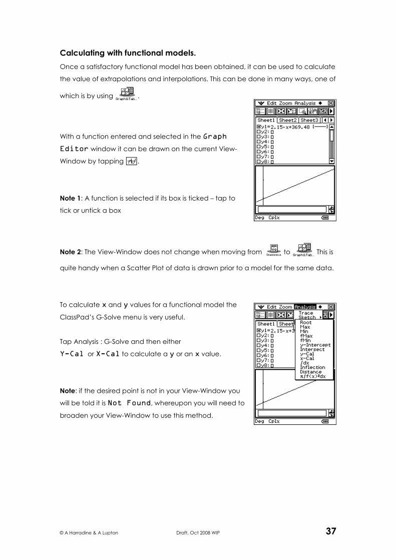
Calculating with functional models.
Once a satisfactory functional model has been obtained, it can be used to calculate
the value of extrapolations and interpolations. This can be done in many ways, one of
which is by using W.
With a function entered and selected in the Graph
Editor window it can be drawn on the current View-
Window by tapping $.
Note 1: A function is selected if its box is ticked – tap to
tick or untick a box
Note 2: The View-Window does not change when moving from I to W This is
quite handy when a Scatter Plot of data is drawn prior to a model for the same data.
To calculate x and y values for a functional model the
ClassPad’s G-Solve menu is very useful.
Tap Analysis : G-Solve and then either
Y-Cal or X-Cal to calculate a y or an x value.
Note: if the desired point is not in your View-Window you
will be told it is Not Found, whereupon you will need to
broaden your View-Window to use this method.
© A Harradine & A Lupton Draft, Oct 2008 WIP 38
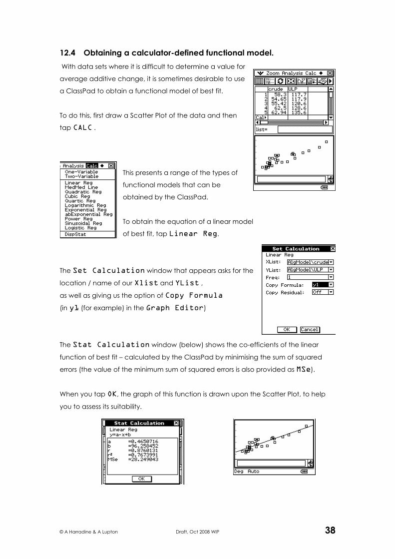
12.4 Obtaining a calculator-defined functional model.
With data sets where it is difficult to determine a value for
average additive change, it is sometimes desirable to use
a ClassPad to obtain a functional model of best fit.
To do this, first draw a Scatter Plot of the data and then
tap CALC .
This presents a range of the types of
functional models that can be
obtained by the ClassPad.
To obtain the equation of a linear model
of best fit, tap Linear Reg.
The Set Calculation window that appears asks for the
location / name of our Xlist and YList ,
as well as giving us the option of Copy Formula
(in y1 (for example) in the Graph Editor)
The Stat Calculation window (below) shows the co-efficients of the linear
function of best fit – calculated by the ClassPad by minimising the sum of squared
errors (the value of the minimum sum of squared errors is also provided as MSe).
When you tap OK, the graph of this function is drawn upon the Scatter Plot, to help
you to assess its suitability.
© A Harradine & A Lupton Draft, Oct 2008 WIP 39
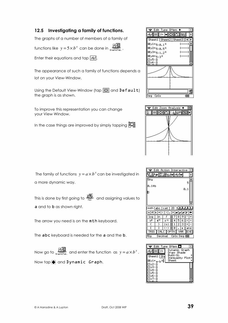
12.5 Investigating a family of functions.
The graphs of a number of members of a family of
functions like xby ×= 5 can be done in W.
Enter their equations and tap $.
The appearance of such a family of functions depends a
lot on your View-Window.
Using the Default View-Window (tap 6 and Default)
the graph is as shown.
To improve this representation you can change
your View Window.
In the case things are improved by simply tapping r
The family of functions xbay ×= can be investigated in
a more dynamic way.
This is done by first going to J and assigning values to
a and to b as shown right.
The arrow you need is on the mth keyboard.
The abc keyboard is needed for the a and the b.
Now go to W and enter the function as xbay ×= .
Now tap ~ and Dynamic Graph.
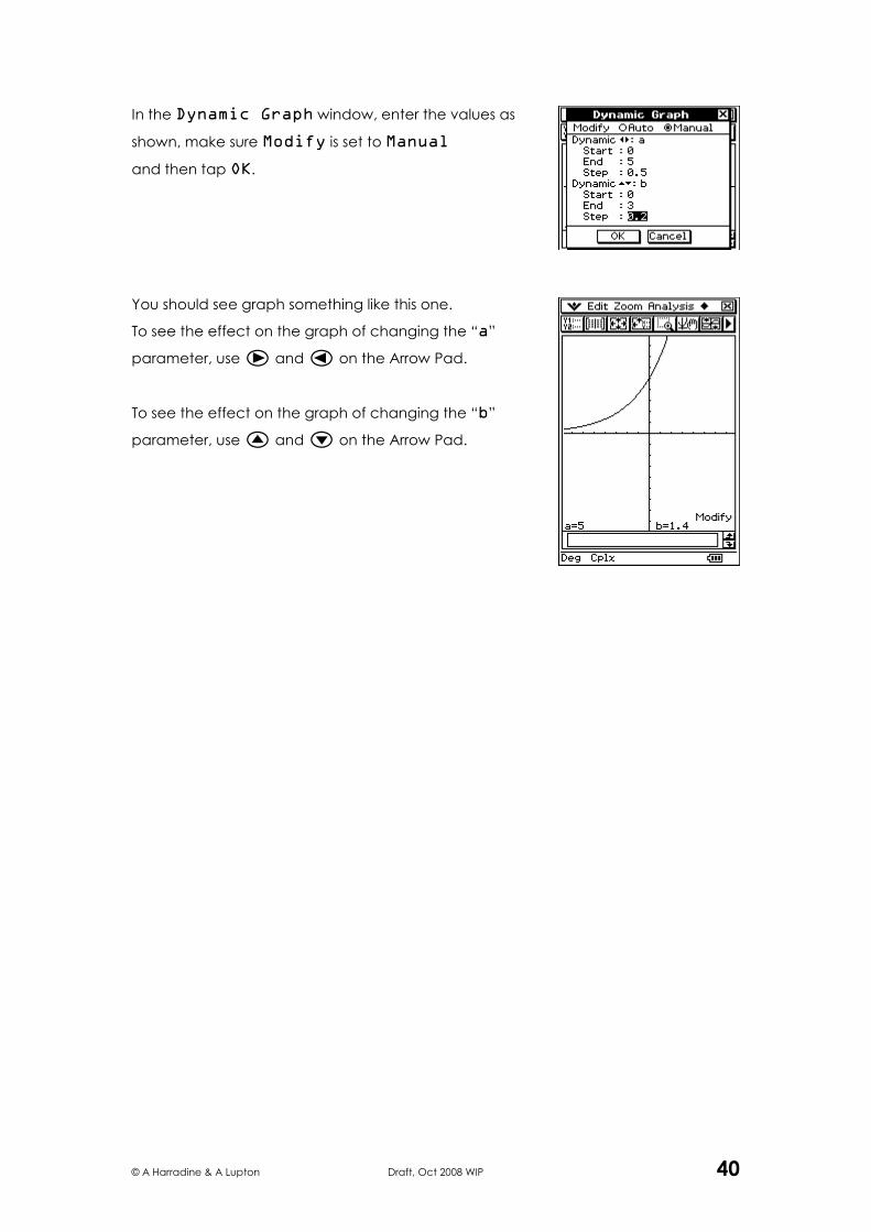
© A Harradine & A Lupton Draft, Oct 2008 WIP 40
In the Dynamic Graph window, enter the values as
shown, make sure Modify is set to Manual
and then tap OK.
You should see graph something like this one.
To see the effect on the graph of changing the “a”
parameter, use e and d on the Arrow Pad.
To see the effect on the graph of changing the “b”
parameter, use f and c on the Arrow Pad.

© A Harradine & A Lupton Draft, Oct 2008 WIP 41
13. Answers.
4.1 Can you ….1.
1. 360180 −= nA
2. a. 180
b.
This value represents
the increase in internal
angle sum upon the
addition of a side to a
polygon.
3.
An axis intercept of
360− means that,
according to this
relationship, a polygon
with no sides would
have an internal angle
sum of o360−
(a somewhat “un-real”
result).
4.
o
A
1800
36012180
=
−×=
5.
...33.11
3601801680
=⇒
−=
n
n
But Zn ∈ (as polygons
only have whole
numbers of sides).
6.
Rely of the fact that
the sum of the interior
angles of a triangle is o180 .
5.1
1. t - the length of the
loan in years – is the
explanatory variable.
A - the amount owed
in $ - is the response
variable.
2.
t A
0 5400
1 5616
2 5832
3 6048
4 6264
5 6480
3.
For each addition of
one year there is an
addition of a fixed
amount ($216) to the
amount owed.
4.
If you consider only
whole years
If you consider interest
accruing over
continuous time
5.
5400216 += tA
6.
a.
7560$
540010216
=
+×
b. 7074$
7.
3216
90005400216
=⇒
=+
t
t
(i.e. 16 years and 8
months).
5.2
1.
A constant adder in K
(i.e. 36) for a constant
adder in M (i.e. 10).
2. MK 6.3= .
3. a. 96.66 km/h
b. 4320 km/h
c. 3216 m/s
d. 18143 m/s
5.3
1.
This shows the 4 points
This better captures
the relationship.
2. 9
5
20
9
100
= .
3. 9
16095 −= FC
4. a.
o
C
35
959
16095
=
−×=
b. o
92182
5. 32
59
9160
95
+=∴
+=
CF
CF
6. a Fo32
b Fo104
© A Harradine & A Lupton Draft, Oct 2008 WIP 42
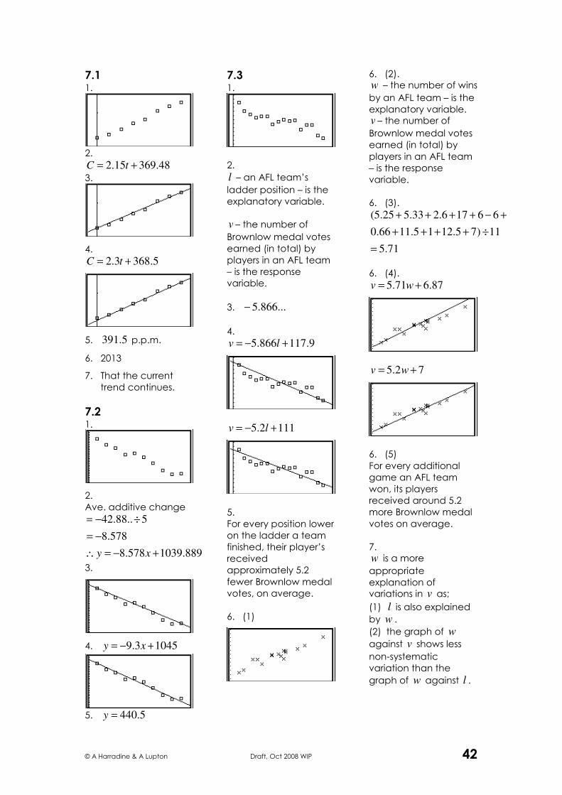
7.1 1.
2.
48.36915.2 += tC
3.
4.
5.3683.2 += tC
5. 5.391 p.p.m.
6. 2013
7. That the current
trend continues.
7.2 1.
2.
Ave. additive change
889.1039578.8
578.8
5..88.42
+−=∴
−=
÷−=
xy
3.
4. 10453.9 +−= xy
5. 5.440=y
7.3 1.
2.
l – an AFL team’s
ladder position – is the
explanatory variable.
v – the number of
Brownlow medal votes
earned (in total) by
players in an AFL team
– is the response
variable.
3. ...866.5−
4.
9.117866.5 +−= lv
1112.5 +−= lv
5.
For every position lower
on the ladder a team
finished, their player’s
received
approximately 5.2
fewer Brownlow medal
votes, on average.
6. (1)
6. (2). w – the number of wins
by an AFL team – is the
explanatory variable. v – the number of
Brownlow medal votes
earned (in total) by
players in an AFL team
– is the response
variable.
6. (3).
71.5
11)75.1215.1166.0
66176.233.525.5(
=
÷++++
+−++++
6. (4).
87.671.5 += wv
72.5 += wv
6. (5)
For every additional
game an AFL team
won, its players
received around 5.2
more Brownlow medal
votes on average.
7. w is a more
appropriate
explanation of variations in v as;
(1) l is also explained
by w .
(2) the graph of w
against v shows less
non-systematic
variation than the
graph of w against l .
© A Harradine & A Lupton Draft, Oct 2008 WIP 43
7.4
1.
2.
3. 8205000 −= wp
4.
A diamond weighing 1
carat more will cost
$5000 extra.
5.
a. 1430$
b. 1930$
c. 564.0 carats.
7.5
1. c - the cost of a barrel
of crude oil in US dollars
is the explanatory
variable.
p - the price of a litre
of ULP in Australian
cents is the response
variable.
2.
96465.0 += cp
3. The “rule of thumb”
suggests that the
model should have an
adder of approx. 1.
The model has an
adder of around 5.0 .
As such, a much better
rule of thumb would be
that a one dollar
increase in the barrel
price of crude oil adds
half a cent per litre to
the price of ULP.
8.1
1.
To increase x by %6 is
to add %6 of x to x
i.e.
06.1
)1(
1006
1006
×=
+=
÷×+
x
x
xx
2. a. Increase by %45
b. Increase by %5.2
c. Decrease by %5
d. Decrease by
%5.17 .
3.
a. nV )085.1(6250=
b. nV )0225.1(92.14=
c. nV )11.1(115000=
10.1
1. R
M 62.312.4 ×=
2. 111046.7 × MJ
3. 141046.7 × MJ
4.
A ‘quake measuring
two more on the
Richter scale releases
1000 times as much
energy!
10.2
1.
A multiplier of 85.0
means depreciation by
%15 per year.
2. t
V 85.0112500 ×=
3. a. 37.22148$
b. 30.12540$
4. The 20th year.
10.3
1.
971.0
89.04
=∴
=
b
b
This represents decay
of %9.2 per day.
2. t
W 971.0100 ×=
3. a. 38.81 grams
b. 0022.0 grams
4.
6.23
5.0971.0
=⇒
=
t
t
.
10.4
1. 259.1
2. d
I 259.110 12×=
−
3. a. 7104 −
×
b. 0318.0
10.5
1.
03.19643$
015.11000 200
=
×
2. t
V 005.11000 ×=
3. 90.19935$
4. t
V 000164.11000 ×=
59.20080$
5.
Value compounded
quarterly = 44.2$
monthly = 61.2$
daily = 714567.2$
second = 718281.2$
Compounded
continuously the value
...597182818284.2== e
© A Harradine & A Lupton Draft, Oct 2008 WIP 44
11.1
1.
2.
The flow decreases
rapidly at first, then
more slowly.
Given the context the
flow should decay to
zero.
3. 883.0
4. t
F 883.07.51 ×=
tF 87.07.51 ×=
5.
77.16=t
i.e about three quarters
the way through
October 1999.
7.
As the flow for October
was below 5 MMscf/d
the well was needed in
that month.
8.
The increase in flow
suggests the well was
ready in November.
9. 10905.05.31 −
×=t
F
When 29=t , 5<f
i.e November 2001.
11.2
1.
Adders in 1=n
Multipliers in =H …
2.
3. n
H 849.010×=
4.
5. As n , the bounce
number, must be a
positive integer, no
additional heights can
be interpolated
between bounce 0
and bounce 14
6. 37.0 metres
7. The 29th bounce.
11.3
1.
2. 026.1
3.
8.79
026.12.103 10
=
÷
Hence xy 026.18.79 ×=
4.
5. xy 027.178×=
6. 8.151
11.4
1.
2.
Because there is no
constant adder in
internet use .
Because the scatter
plot is curved!
3.
The “best” simple
exponential model that
can be obtained is
something like t
W 34.193.0 ×=
But this model fits the
data very poorly
© A Harradine & A Lupton Draft, Oct 2008 WIP 45
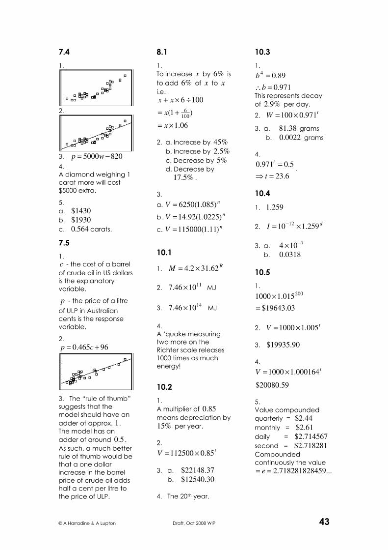
The reason that there is
no better model of this
type is that the data
does not have an
approximate constant
multiplier.
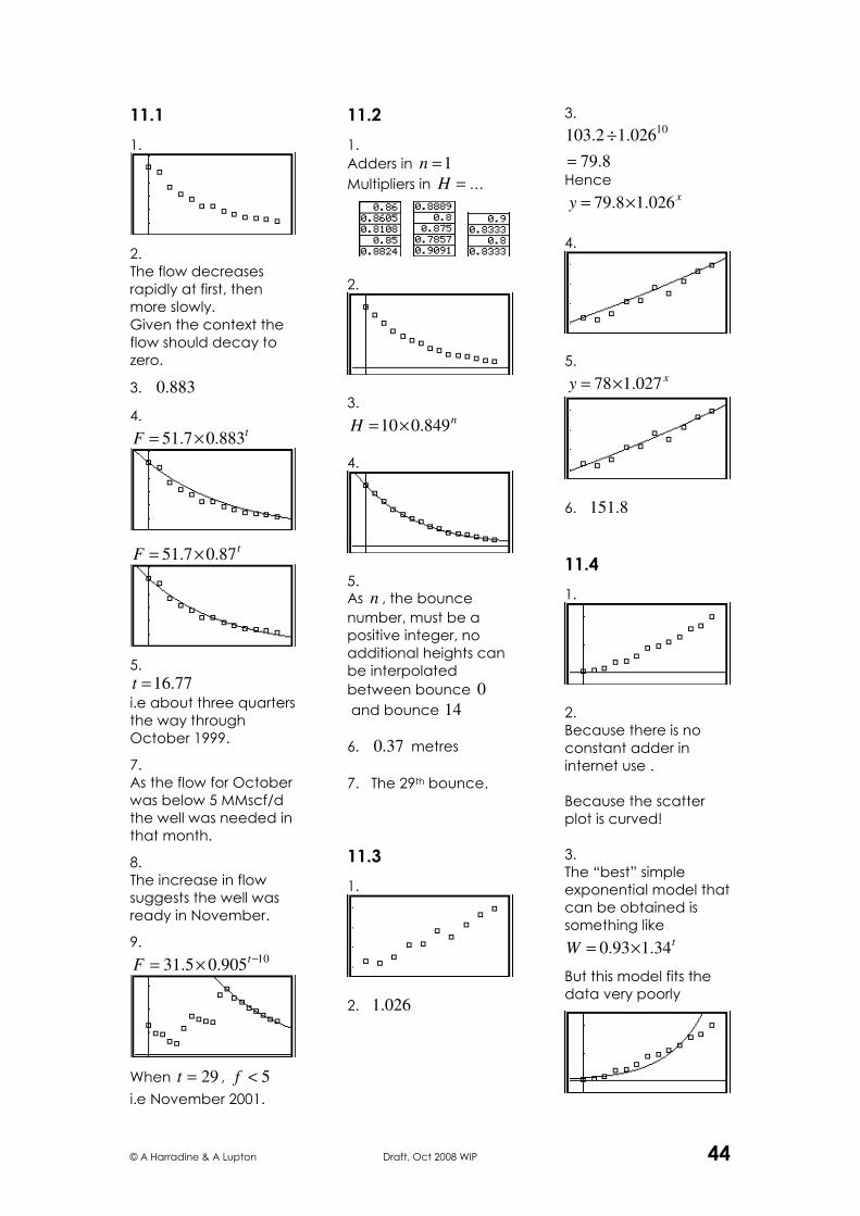
4.
5. In 2012.
6. There is a good
chance that the
prediction will be
inaccurate as there
may not be another
13% of the world’s
population ready to
take up internet use
(i.e. the trend of
increasing growth may
be unable to
continue).