Depth to Magnetic Basement of the Capel and Faust Basins ... · Depth to magnetic basement of the Capel and Faust Basins 3 Figure 1. Location of the ship track profiles from survey

Goutam Kumar Nayak and Peter Petkovic

Record

2011/42

Depth to Magnetic Basement of the Capel and Faust Basins, Lord Howe Rise

GeoCat # 71844

APPLYING GEOSCIENCE TO AUSTRALIA’S MOST IMPORTANT CHALLENGES

G E O S C I E N C E A U S T R A L I A

Depth to Magnetic Basement of the Capel and Faust Basins, Lord Howe Rise GEOSCIENCE AUSTRALIA RECORD 2011/42 by Goutam Kumar Nayak and Peter Petkovic

Petroleum & Marine Division, Geoscience Australia GPO Box 378, Canberra, ACT, 2601 CANBERRA 2011

Department of Resources, Energy and Tourism Minister for Resources and Energy: The Hon. Martin Ferguson, AM MP Secretary: Mr Drew Clarke Geoscience Australia Chief Executive Officer: Dr Chris Pigram

© Commonwealth of Australia (Geoscience Australia) 2011 With the exception of the Commonwealth Coat of Arms and where otherwise noted, all material in this publication is provided under a Creative Commons Attribution 3.0 Australia Licence (www.creativecommons.org/licenses/by/3.0/au/) Geoscience Australia has tried to make the information in this product as accurate as possible. However, it does not guarantee that the information is totally accurate or complete. Therefore, you should not solely rely on this information when making a commercial decision. ISSN 1448-2177 ISBN 978-1-921954-52-9 GeoCat No. 71844 Bibliographic reference: Nayak, G.K. and Petkovic, P. 2011. Depth to magnetic basement of the Capel and Faust Basins, Lord Howe Rise. Record 2011/42. Geoscience Australia: Canberra.

Depth to magnetic basement of the Capel and Faust Basins

iii

Contents

Executive Summary ..........................................................................................................................1

Introduction.......................................................................................................................................2

Data Acquisition and Processing ......................................................................................................4

Gridding and Reduction to the Pole ..................................................................................................5

Depth to Magnetic Basement ............................................................................................................7

Spectral Analysis Method .........................................................................................................7

Error Analysis .................................................................................................................................13

Comparison with Reflection Seismic Model ..................................................................................17

Conclusions.....................................................................................................................................21

Acknowledgements.........................................................................................................................21

References.......................................................................................................................................22


iv


1

Executive Summary

As a part of the Australian Government’s Energy Security programme, Geoscience Australia

acquired pre-competitive ship-borne geophysical data over the Capel and Faust basins, about

800 km east of Brisbane. Marine surveys GA-302 and GA-2436 were conducted during 2006 and

2007, over an area of more than 100,000 km2, at water depths of 1000–3000 m to acquire

reflection and refraction seismic, swath bathymetry, gravity and magnetic data.

This document describes how magnetic spectra were used in an attempt to estimate depth to

magnetic basement and give additional constraint on the basement architecture of these frontier

basins where seismic coverage is sparse and there is only one shallow well. A semi-automated

method was developed using a combination of commercial and in-house developed software in

order to improve the utility of the spectral method.

The results confirm the seismic interpretation of a substantial depocentre, about 6 km thickness

trending north-northwest in the northwest part of the Capel and Faust Basins study area. The

magnetic analysis indicate the presence of a north trending ridge in the central part of the study

area, also evident in the reflection seismic data.

The results indicate that our semi-automated magnetic spectral method is viable and points to

areas where it can be improved. We propose the technique may be useful in the study of other

frontier basins where the magnetic data coverage is of comparable detail and resolution.


2

Introduction

The Capel and Faust basins of the Lord Howe Rise were surveyed during 1996 and 1998 as part of

Geoscience Australia’s Law of the Sea programme to define Australia’s legal continental shelf

margin. The data from these surveys indicated that sediment pockets existed (Ramsay et al., 1997,

Bernardel et al., 1999) creating interest in the region as a possible petroleum province (Stagg et

al., 1999), although it was unclear just how extensive and thick the sediments were.

Geoscience Australia completed a seismic survey (GA-302) of these basins during the summer of

2006/07 to explore the area in detail, using 2D acquisition technology to image the sedimentary

sequences and the underlying crust. The survey was conducted on behalf of Geoscience Australia

by Compagnie Générale de Géophysique (now CGG Veritas) on the platform Pacific Titan,

collecting 5920 km of high-quality 106 fold 2D seismic reflection data to 12 s two-way travel time

at 37.5 m shot interval using an 8 km streamer (Compagnie Générale de Géophysique, 2007), as

well as magnetic, gravity, bathymetry and sonobuoy refraction data. The potential field and

bathymetry data were processed by Fugro Robertson (2007). The reflection seismic data from this

survey was interpreted by Colwell et al. (2010) and the refraction data by Petkovic (2010).

Following survey GA-302 in 2007, Geoscience Australia survey GA-24361 collected multi-beam

bathymetry data and sea-floor samples as well as magnetic and gravity data over the northwest

part of the GA-302 survey area at a 4 km line spacing (Heap et al., 2009). The location of surveys

GA-302 and GA-2436 is shown in Figure 1. The potential field and bathymetry data on this survey

were acquired and processed by Fugro Robertson (2008).

1 GA-2436 is also known by the acquisition platform name “R/V Tangaroa” or the National Institute of Water & Atmospheric Research (New Zealand) code TAN-713.


3

Figure 1. Location of the ship track profiles from survey GA-302, sonobuoys from GA-302 [ red segments on seismic lines], two lines from earlier survey GA-206, the location of DSDP 208 [ ], pre-existing velocity models [ ], and closely spaced lines from multi-beam bathymetry and potential field survey GA-2436 (also known as ‘Tangaroa’ survey). Bathymetric contours are background.

The results of stratigraphic studies using reflection seismic data from GA-302 are reported in

Colwell et al. (2010), who supported earlier notions (e.g. Gaina et al., 1998; van de Beuque et al.,

2003) that the Lord Howe Rise is underlain in this region by continental crust which was part of

greater Australia before its Late Cretaceous breakup and the formation of the Tasman Sea.

Reflection seismic data from GA-302 provides evidence for this proposition by the variable


4

character of basement which includes both characterless transparent zones and sections where

layering is clearly present, indicative of intruded and altered older Mesozoic basins. In addition,

Colwell et al. (2010) opined that the entire seismic stratigraphic sequence is intruded or

interbedded with volcanic sills and dykes throughout the sedimentary succession. Thus, at the

outset of the study it remained difficult to determine sediment thickness, one of the fundamental

parameters of petroleum potential, despite the high quality seismic data and adequate penetration

of seismic energy. To test various seismic basement depth ideas Petkovic (2008) and Petkovic et

al. (2011) developed 2.5D and 3D gravity models using sediment and basement densities inferred

from velocity models of refraction data.

This study focuses on the magnetic data and describes the method for estimating depth to

magnetic basement on the assumption that the basement is composed of randomly distributed

magnetic sources. It provides an independent estimate of sediment thickness, alongside the

refraction and reflection seismic models and the gravity models.

Data Acquisition and Processing Total magnetic field measurements were acquired on surveys GA-302 and GA-2436 using a

proton precession SeaSpy marine magnetometer towed between 210 and 245 m astern by a

floating tow cable and recorded at 1 second intervals. The magnetometer head was towed at least

two ship lengths astern to avoid recording the magnetic field of the ship (Bullard & Mason, 1961).

The GA-302 and GA-2436 datasets were processed by Fugro Robertson Inc LCT Gravity and

Magnetics Division (Fugro Robertson) and provided to Geoscience Australia in the first half of

2008. Processing involved:

position correction for the distance between sensor and navigation antenna,

subtraction of the International Geomagnetic Reference Field (IGRF) value extrapolated

from the 2005 formula,

diurnal correction,

filtering using a Butterworth filter with a cutoff at 60 seconds2, and

network adjustment to minimise misties.

2 ship speed on GA-302 was ~150 m/minute and GA-2436 ~300 m/minute


5

The network adjustment reduced mistie rms from 10.1 nT (before adjustment) to 5.6 nT for survey

GA-302 and from 8.8 nT to 1.3 nT for survey GA-2436.

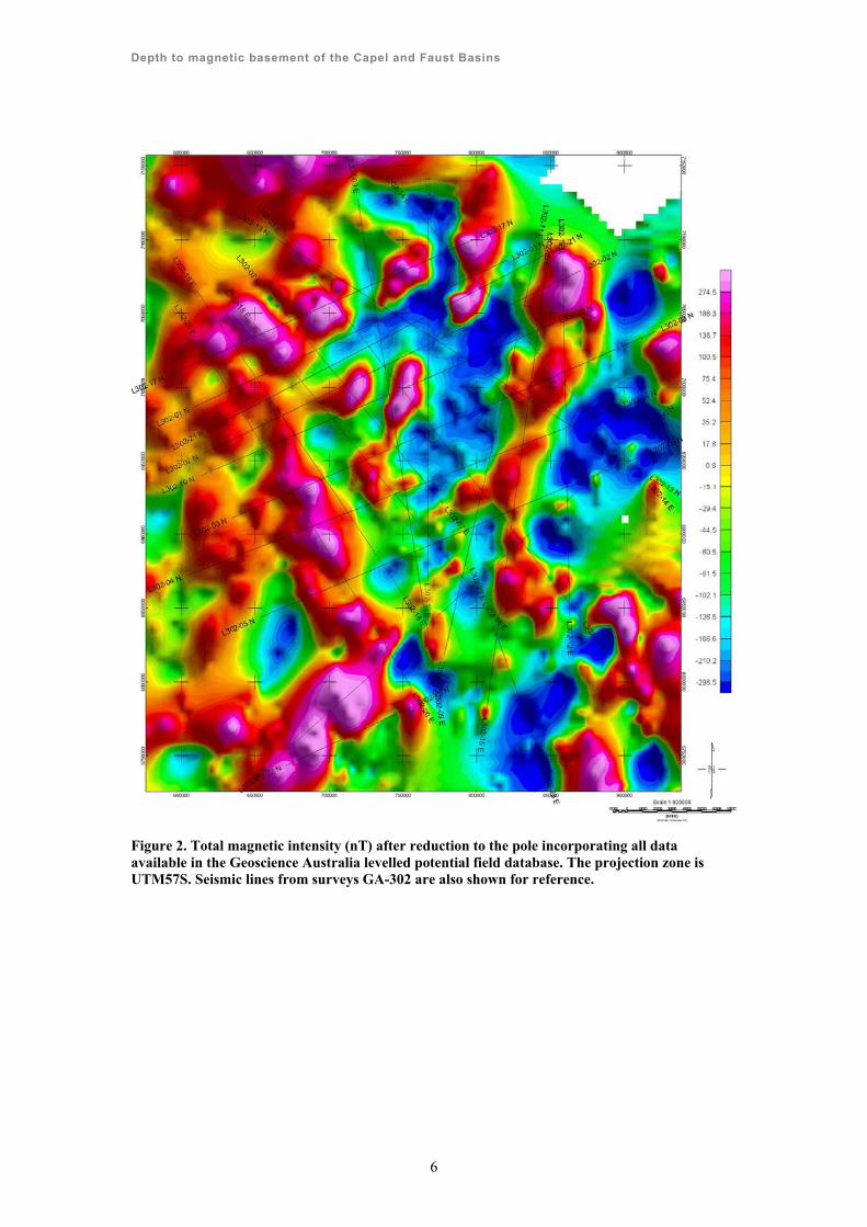
The magnetic line data from each survey were gridded with a cell-size of 0.01º using minimum

curvature technique and merged with grids from data obtained on earlier surveys (Hackney, 2010).

Figure 2 shows the reduced to pole anomaly with respect to the IGRF of the integrated dataset,

which was the basis for estimating depth to magnetic basement.

Gridding and Reduction to the Pole

The IGRF-corrected total magnetic intensity (TMI) profile data were gridded with 5000 m grid

cell size using the minimum curvature algorithm with Oasis MontajTM software. This cell size

minimises gaps in the grid image of the area where the approximate line separation for GA-302 is

40 km and 4 km for GA-2436 in the northwest of the study area (Figure 1).

The measured magnetic field at any point is the combination of the Earth’s magnetic field and the

field due to crustal induced and remnant magnetisation. It will be assumed that the remnant

magnetisation is in the direction of induced magnetisation or the magnitude of remnant

magnetisation is small compared to the induced magnetisation. Except at the magnetic poles,

where the Earth’s magnetic field is vertical, the anomaly due to the induced magnetisation will be

displaced away from the bodies that cause them. To restore the position of anomalies, a reduction-

to-pole process (RTP) was applied (Figure 2) and is the basic data set for all depth computation in

the following sections.


6

Figure 2. Total magnetic intensity (nT) after reduction to the pole incorporating all data available in the Geoscience Australia levelled potential field database. The projection zone is UTM57S. Seismic lines from surveys GA-302 are also shown for reference.


7

Depth to Magnetic Basement

The basement rocks of sedimentary basins commonly consist of igneous or metamorphic rocks,

while the overlying sediments are non-magnetic. This means that the interface between the

basement and the sediments represents a strong magnetic contrast. In such cases the depth to

magnetic sources determination by magnetic methods gives reliable estimates of the depth to

geological basement. In the present case the situation is complicated because the geological

basement is believed to consist of older sedimentary basin material and the overlying sedimentary

pile shows evidence of magmatic intrusion. Nevertheless we conducted magnetic depth estimation

and compared the results to depths derived from reflection seismic data by Colwell et al. (2010).

We used the spectral method of Spector and Grant (1970) which works best in situations where

magnetic anomalies are due to randomly distributed sources.

Spectral Analysis Method

Magnetic depth estimation methods such as Euler and Werner deconvolution don’t work well in

areas where magnetic anomalies represent the superposition of individual anomalies from multiple

discrete bodies. In such cases, power spectrum analysis of the magnetic data can be used to

estimate an ensemble average depth to magnetic marker horizons which separate two different sets

of randomly distributed magnetic source bodies (Spector and Grant, 1970). In the present case we

assumed magnetic anomalies are caused by:

sources of magnetic materials lying within the sedimentary succession, and/or

possible magnetic rocks present within the basement (up to Curie isotherm).

The magnetic power spectrum method, which does not use magnetic field gradients, allows an

interpreter to separate magnetic signatures arising from magnetic horizons lying at different

depths. These will appear as discrete straight line segments on log-power vs frequency plots. The

slopes of these segments are a function of the depth to the top of magnetic marker horizons.

The process is described as follows: the RTP-corrected grid (Figure 2) was smoothed by upward

continuation to 500 m then split into 50 km x 50 km sub-grids with 90% overlap (centres 5 km

apart) using program ‘splitdomain3’. The size of the sub-grid determines the frequency content in

the spectrum and hence the depth of investigation. Nayak and Rama Rao (2002) and Odegard and

3 ‘splitdomain’ is an in-house program written in Fortran by Indrajit Roy


8

Weber (2005) working on sedimentary basins in different parts of the world suggested that a

window of 45–55 km was optimum for investigating depth to basement. We calculated the power

spectrum for each 50 km x 50 km sub-grid, of which there were ~7000, using the Fast Fourier

Transform (FFT) in the IntrepidTM software run in batch mode. The radially averaged energy

spectrum was calculated for each window by averaging the energy from all directions for the same

wavenumber. The results (wavenumber vs energy) were tabulated to one output text file per

window so that a plot of the result for each window could be inspected and slopes determined.

The slope of the straight line fit to the plot of the wavenumbers (cycles/meter) versus the energy

(log P) is proportional to the ensemble average depth to the different magnetic marker horizons.

The depth to the magnetic marker is given by:

N

Eh

4

1

where,

E = Energy in log power,

N = Frequency/wave-number, and

∆E/∆N is the slope of the straight line segment of the spectrum.

To compute the depth from the energy spectrum for each of ~7000 power spectrum reports we

developed an approach to automate the slope determination process. The tabulations of ∆E and ∆N

were read into program ‘powerspec_rpt_fixed.pl’ which computed the slope of the line of least-

squares best fit between user specified fixed lower and upper values of N. To determine this

frequency band ten windows were randomly selected and depth to basement determined manually

for each (Table 1). By inspection, basement lay in the 0.015 to 0.095 cycle/km band which was

then given as the program parameter.

A companion program, ‘powerspec_rpt_variable.pl’, computed the slope from a fixed lower

frequency (0.015 km-1, as did powerspec_rpt_fixed.pl) to a variable upper frequency. The upper

frequency was determined for each window using a change-of-slope search algorithm.


9

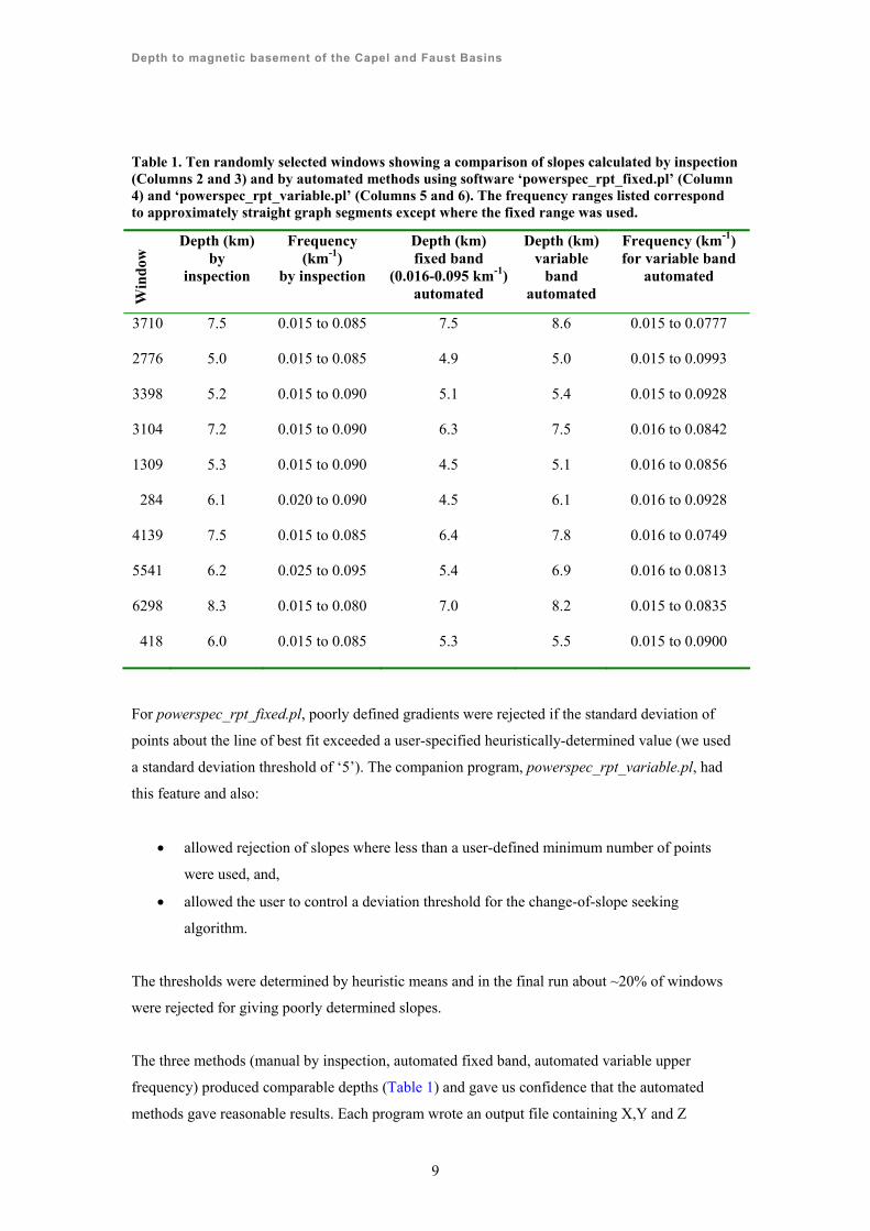
Table 1. Ten randomly selected windows showing a comparison of slopes calculated by inspection (Columns 2 and 3) and by automated methods using software ‘powerspec_rpt_fixed.pl’ (Column 4) and ‘powerspec_rpt_variable.pl’ (Columns 5 and 6). The frequency ranges listed correspond to approximately straight graph segments except where the fixed range was used.

Win

dow

Depth (km) by

inspection

Frequency (km-1)

by inspection

Depth (km) fixed band

(0.016-0.095 km-1)automated

Depth (km) variable

band automated

Frequency (km-1) for variable band

automated

3710 7.5 0.015 to 0.085 7.5

8.6

0.015 to 0.0777

2776 5.0 0.015 to 0.085 4.9

5.0 0.015 to 0.0993

3398 5.2 0.015 to 0.090 5.1

5.4 0.015 to 0.0928

3104 7.2 0.015 to 0.090 6.3

7.5 0.016 to 0.0842

1309 5.3 0.015 to 0.090 4.5

5.1 0.016 to 0.0856

284 6.1 0.020 to 0.090 4.5

6.1 0.016 to 0.0928

4139 7.5 0.015 to 0.085 6.4

7.8 0.016 to 0.0749

5541 6.2 0.025 to 0.095 5.4

6.9 0.016 to 0.0813

6298 8.3 0.015 to 0.080 7.0

8.2 0.015 to 0.0835

418 6.0 0.015 to 0.085 5.3

5.5 0.015 to 0.0900

For powerspec_rpt_fixed.pl, poorly defined gradients were rejected if the standard deviation of

points about the line of best fit exceeded a user-specified heuristically-determined value (we used

a standard deviation threshold of ‘5’). The companion program, powerspec_rpt_variable.pl, had

this feature and also:

allowed rejection of slopes where less than a user-defined minimum number of points

were used, and,

allowed the user to control a deviation threshold for the change-of-slope seeking

algorithm.

The thresholds were determined by heuristic means and in the final run about ~20% of windows

were rejected for giving poorly determined slopes.

The three methods (manual by inspection, automated fixed band, automated variable upper

frequency) produced comparable depths (Table 1) and gave us confidence that the automated

methods gave reasonable results. Each program wrote an output file containing X,Y and Z


10

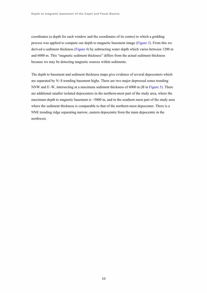
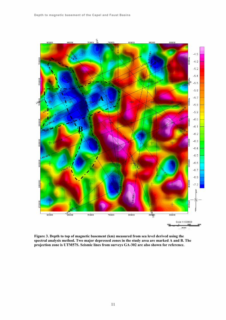
coordinates (a depth for each window and the coordinates of its centre) to which a gridding

process was applied to compute our depth to magnetic basement image (Figure 3). From this we

derived a sediment thickness (Figure 4) by subtracting water depth which varies between 1200 m

and 6000 m. This “magnetic sediment thickness” differs from the actual sediment thickness

because we may be detecting magnetic sources within sediments.

The depth to basement and sediment thickness maps give evidence of several depocenters which

are separated by N–S trending basement highs. There are two major depressed zones trending

NNW and E–W, intersecting at a maximum sediment thickness of 6000 m (B in Figure 3). There

are additional smaller isolated depocenters in the northern-most part of the study area, where the

maximum depth to magnetic basement is ~5000 m, and in the southern most part of the study area

where the sediment thickness is comparable to that of the northern-most depocenter. There is a

NNE trending ridge separating narrow, eastern depocentre from the main depocentre in the

northwest.


11

Figure 3. Depth to top of magnetic basement (km) measured from sea level derived using the spectral analysis method. Two major depressed zones in the study area are marked A and B. The projection zone is UTM57S. Seismic lines from surveys GA-302 are also shown for reference.

A

B


12

Figure 4. Sediment thickness derived by subtracting the bathymetry from magnetic basement depth (km). The projection zone is UTM57S.


13

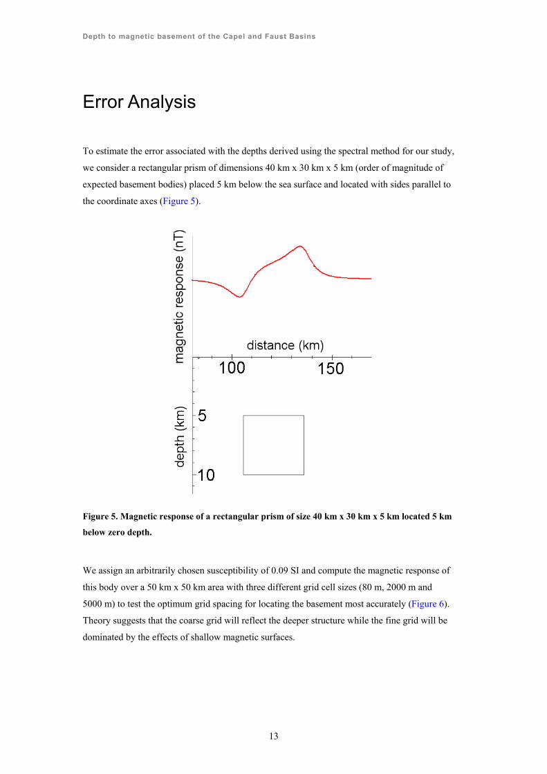
Error Analysis

To estimate the error associated with the depths derived using the spectral method for our study,

we consider a rectangular prism of dimensions 40 km x 30 km x 5 km (order of magnitude of

expected basement bodies) placed 5 km below the sea surface and located with sides parallel to

the coordinate axes (Figure 5).

Figure 5. Magnetic response of a rectangular prism of size 40 km x 30 km x 5 km located 5 km

below zero depth.

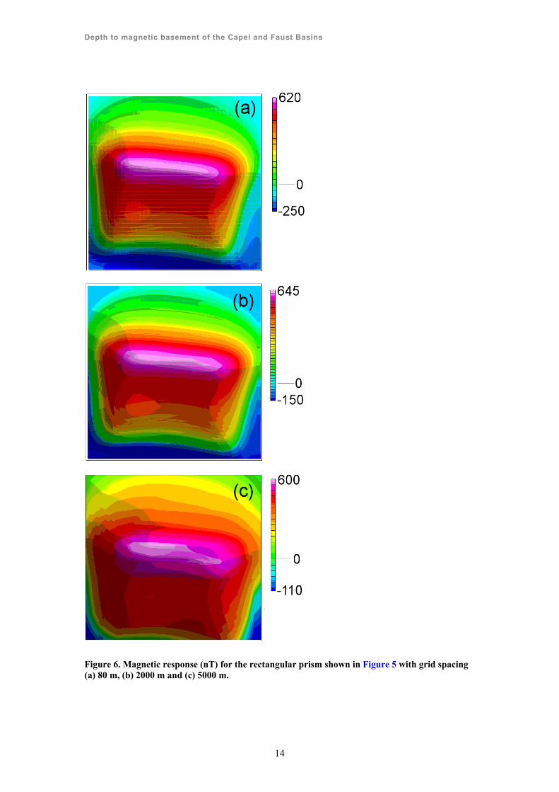
We assign an arbitrarily chosen susceptibility of 0.09 SI and compute the magnetic response of

this body over a 50 km x 50 km area with three different grid cell sizes (80 m, 2000 m and

5000 m) to test the optimum grid spacing for locating the basement most accurately (Figure 6).

Theory suggests that the coarse grid will reflect the deeper structure while the fine grid will be

dominated by the effects of shallow magnetic surfaces.


14

Figure 6. Magnetic response (nT) for the rectangular prism shown in Figure 5 with grid spacing (a) 80 m, (b) 2000 m and (c) 5000 m.


15

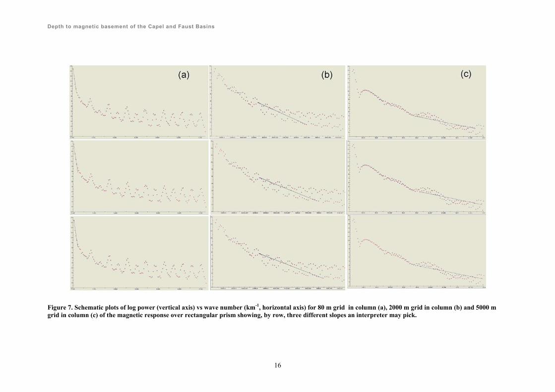
Figure 7a represents the power spectrum for the 80 m grid-spacing. We consider three different

slopes that may be picked within the frequency band 4.2 to 19.9 x 10-5 cycle/km. The average

depth from these is 4700 m with a range of 4600–4800m, and the average depth is in error by

~6%.

Similarly, Figure 7b and Figure 7c represent three different slopes that may be used to compute

the depth for the grid spacing 2000 m and 5000 m respectively. In Figure 7a and Figure 7b the top

of basement lies in a common frequency band of 4.2 to 20.0 x 10-5 cycle/km. Figure 7a is mostly

dominated by high frequency noise and Figure 7b is almost equally dominated by high and low

frequency noise.

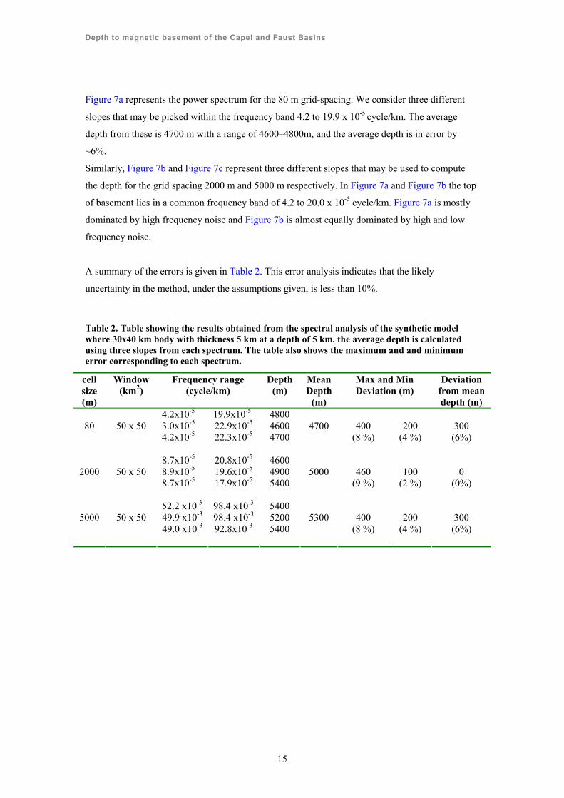
A summary of the errors is given in Table 2. This error analysis indicates that the likely

uncertainty in the method, under the assumptions given, is less than 10%.

Table 2. Table showing the results obtained from the spectral analysis of the synthetic model where 30x40 km body with thickness 5 km at a depth of 5 km. the average depth is calculated using three slopes from each spectrum. The table also shows the maximum and and minimum error corresponding to each spectrum.

cell size (m)

Window (km2)

Frequency range (cycle/km)

Depth (m)

Mean Depth

(m)

Max and Min Deviation (m)

Deviation from mean depth (m)

4.2x10-5 19.9x10-5 4800 3.0x10-5 22.9x10-5 4600

80

50 x 50

4.2x10-5 22.3x10-5 4700

4700 400

(8 %)

200 (4 %)

300 (6%)

8.7x10-5 20.8x10-5 4600 8.9x10-5 19.6x10-5 4900

2000

50 x 50

8.7x10-5 17.9x10-5 5400

5000

460

(9 %)

100

(2 %)

0

(0%)

52.2 x10-3 98.4 x10-3 5400 49.9 x10-3 98.4 x10-3 5200

5000

50 x 50

49.0 x10-3 92.8x10-3 5400

5300

400

(8 %)

200

(4 %)

300 (6%)


16

Figure 7. Schematic plots of log power (vertical axis) vs wave number (km-1, horizontal axis) for 80 m grid in column (a), 2000 m grid in column (b) and 5000 m grid in column (c) of the magnetic response over rectangular prism showing, by row, three different slopes an interpreter may pick.


17

Comparison with Reflection Seismic Model

Reflection seismic data from survey GA-302 over the Capel and Faust Basins was interpreted by

Colwell et al. (2010), whose identification of top of basement was corroborated by velocity

modelling of sonobuoy data (Petkovic, 2010) and gravity modelling (Petkovic et al. 2011). In this

report the depth to magnetic basement over the Capel and Faust basins was derived independently

using the spectral analysis method, without constraints from these previous studies, in order to

develop and test the method and confirm or negate earlier work.

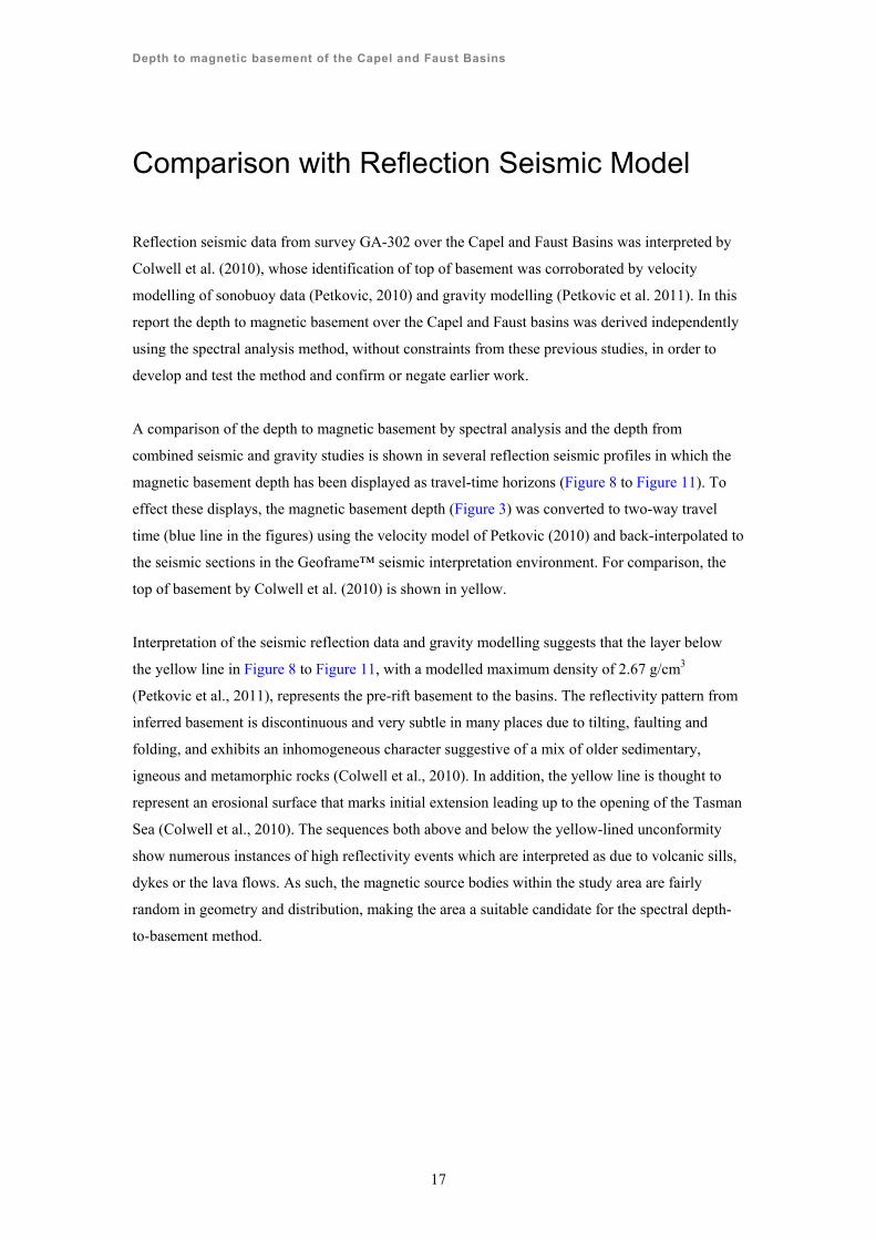
A comparison of the depth to magnetic basement by spectral analysis and the depth from

combined seismic and gravity studies is shown in several reflection seismic profiles in which the

magnetic basement depth has been displayed as travel-time horizons (Figure 8 to Figure 11). To

effect these displays, the magnetic basement depth (Figure 3) was converted to two-way travel

time (blue line in the figures) using the velocity model of Petkovic (2010) and back-interpolated to

the seismic sections in the Geoframe™ seismic interpretation environment. For comparison, the

top of basement by Colwell et al. (2010) is shown in yellow.

Interpretation of the seismic reflection data and gravity modelling suggests that the layer below

the yellow line in Figure 8 to Figure 11, with a modelled maximum density of 2.67 g/cm3

(Petkovic et al., 2011), represents the pre-rift basement to the basins. The reflectivity pattern from

inferred basement is discontinuous and very subtle in many places due to tilting, faulting and

folding, and exhibits an inhomogeneous character suggestive of a mix of older sedimentary,

igneous and metamorphic rocks (Colwell et al., 2010). In addition, the yellow line is thought to

represent an erosional surface that marks initial extension leading up to the opening of the Tasman

Sea (Colwell et al., 2010). The sequences both above and below the yellow-lined unconformity

show numerous instances of high reflectivity events which are interpreted as due to volcanic sills,

dykes or the lava flows. As such, the magnetic source bodies within the study area are fairly

random in geometry and distribution, making the area a suitable candidate for the spectral depth-

to-basement method.


18

Figure 8. Seismic section along line GA302-10. The top of seismic basement (yellow) and magnetic basement converted two-way travel time (blue) are shown. The line is 244.5 km long and the vertical exaggeration is 9.1.

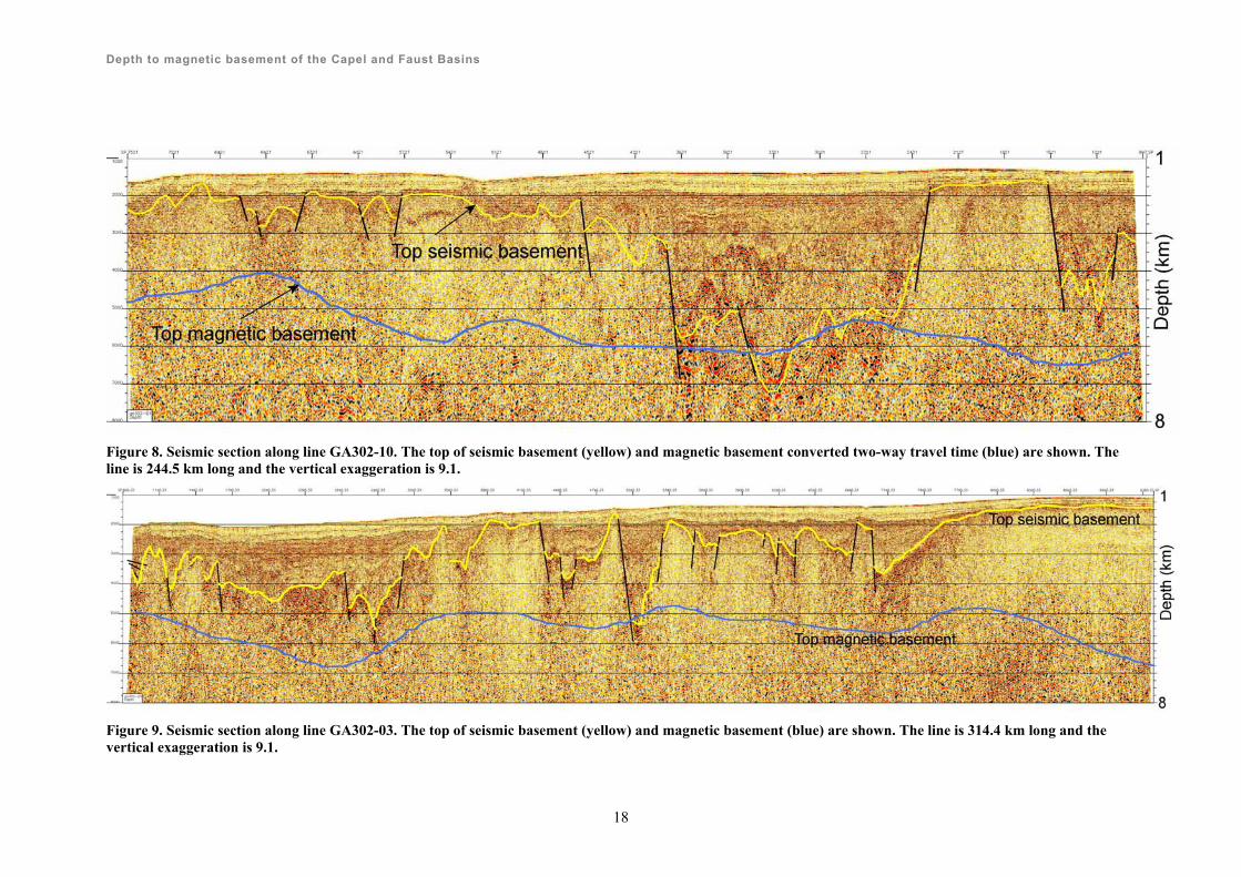
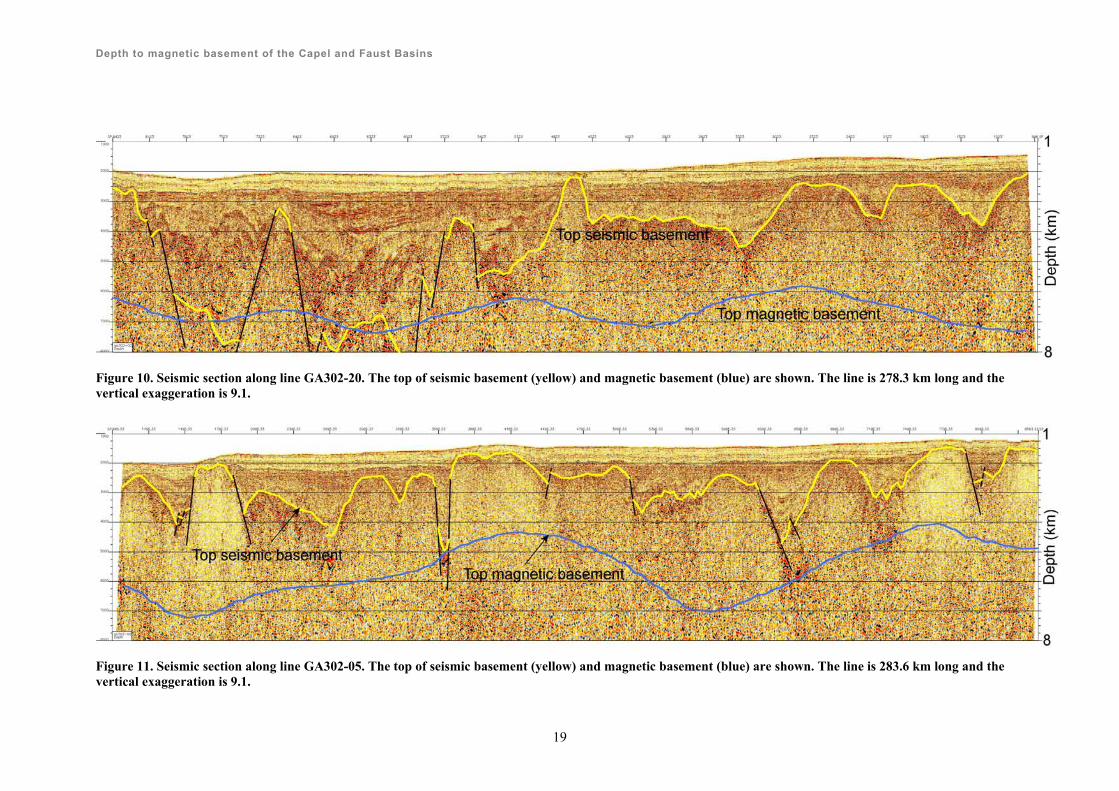
Figure 9. Seismic section along line GA302-03. The top of seismic basement (yellow) and magnetic basement (blue) are shown. The line is 314.4 km long and the vertical exaggeration is 9.1.


19




20

In the representative sections shown in Figure 8 to Figure 11 (above) the basement topography

determined by the two methods are in agreement only in the deeper part of the section, within the

10% error margin predicted from our synthetic example. For example, in Figure 8 and Figure 10

the depths are approximately the same where the seismic basement horizon is at about 7.2 sec two-

way travel time, but at the shallower levels, less than ~5 sec, the two interpretations do not match.

Similarly, in Figure 9 and Figure 11 the seismic interpretation of the central basement-high is at

shallower level compared to the magnetic basement depth.

The greater depths obtained in general by the spectral method outlined in this report may be due

to:

a) an excessively large grid spacing (5000 m) which is not optimum for picking the shallow

magnetic basement surface,

b) the 0.016 to 0.096 frequency band we considered may not be suitable for a shallower

magnetic basement signal, and/or

c) a lack of magnetic materials in the basement of the central high.

The first two points could be addressed by further work, such as using a variable window size in

several passes and developing a better method for automated slope picking of the log power –

frequency plots and error analysis. These methods are currently under investigation by Johnston

and Petkovic (in prep.). A realistic investigation would require use of high performance hardware

combined with fully automated computation for realistic turn-around time, as well as software

development as indicated.

It would then be possible to draw geological conclusions on the thrid point, viz. the degree of

magnetisation and intrusion by magnetic rocks into the shallower parts of what has been

interpreted as basement by reflection and refraction seismic and gravity methods. It would be an

important question to address in order to enhance our understanding of the petroleum potential of

these remote frontier basins.

Despite the discrepancies in depth and lateral offsets obtained by the two methods the power

spectrum method for determining depth to magnetic basement is able to delineate the top of

basement in deeper areas, where the resolution of the seismic is reduced.


21

Conclusions

The results of the magnetic data analysis over the Capel and Faust basins show that the whole area

is divided into a number of sediment depocentres with variable size and shape. The position and

dimensions of the main features agree with earlier work based on seismic and gravity methods.

We can make the following conclusions:

the deepest and most extensive depocenter lies in the northwest of the study area, and

the maximum sediment thickness in the study area is between 5 and 6 km.

Further work could be done to improve the method outlined in this report and allow more

definitive geological conclusions to be drawn.

Acknowledgements

The authors thank Ron Hackney, Indrajit G. Roy, Gabriel Nelson and Stephen Johnston who

reviewed the manuscript, Anne Fleming and Andrea Cortese for assistance with data and

application software, Indrajit Roy for use of the computer program ‘splitdomain’ and Riko

Hashimoto for commentary, criticism and encouragement. The authors publish with the

permission of the Chief Executive Officer, Geoscience Australia.


22

References

Bernardel, G., Lafoy, Y., Van de Beuque, S., Missegue, F. and Nercessian, A. 1999. Preliminary

results from AGSO Law of the Sea Cruise 206: an Australia/French collaborative deep-seismic

marine survey in the Lord Howe Rise/New Caledonia region. Record 1999/14. Australia

Geological Survey Organisation: Canberra.

Bullard, E.C. and Mason, R.G. 1961. ‘The magnetic field astern of a ship’. Deep Sea Research,

8: 20–27.

Colwell, J.B., Hashimoto, T., Rollet, N., Higgins, K.L., Bernardel, G. and McGiveron, S. 2010.

Interpretation of seismic data, Capel and Faust Basins, Australia’s Remote Offshore Eastern

Frontier. Record 2010/06. Geoscience Australia: Canberra. [CD-ROM]

Compagnie Générale de Géophysique, 2007. Final survey report: Capel & Faust basin, MGC Job

No. 6283. Internal report. Geoscience Australia: Canberra.

Fugro Robertson Inc. 2007. Shipborne gravity, magnetic and bathymetric survey data processing

report, L302, Capel and Faust basins, offshore Australia for Geoscience Australia. Internal

report. Geoscience Australia: Canberra.

Fugro Robertson Inc. 2008. Shipborne gravity, magnetic and bathymetric survey data processing

report, Capel and Faust basins, Tangaroa TAN0713, for Geoscience Australia. Internal report.

Geoscience Australia: Canberra.

Gaina, C., Müller, R.D., Royer, J-Y., Stock, J., Hardebeck, J. and Symonds, P. 1998. ‘The tectonic

history of the Tasman Sea: a puzzle with 13 pieces’. Journal of Geophysical Research, 103(B6):

12413–12433.

Hackney, R. 2010. ‘Potential-field data covering the Capel and Faust Basins, Australia's remote

offshore eastern frontier’, Record 2010/34. Geoscience Australia: Canberra.

Heap, A.D., Hughes, M., Anderson, T., Nichol, S., Hashimoto, T., Daniell, J., Przeslawski, R.,

Payne,D., Radke, L. and Shipboard-Party, 2009. Seabed environments and subsurface geology of

the Capel & Faust Basins and Gifford Guyot, Eastern Australia - Geoscience Australia TAN0713

post-survey repor,. Record 2009/22. Geoscience Australia: Canberra.


23

Johnston, S. and Petkovic, P. (in prep.). North Perth Basin 2D and 3D Models of Depth to

Magnetic Basement, Record, Geoscience Australia: Canberra.

Nayak, G.K. and Rama Rao, C. 2002. ‘Structural configuration of Mahanadi offshore basin, India:

an aeromagnetic study’. Marine Geophysical Research, 23(6): 471–479,

doi: 10.1023/B:MARI.0000018244.65222.9a

Odegard, M.E. and Weber, W.R. 2005. Depth to basement using spectral inversion of magnetic

and gravity data: application to Northwest Africa and Brazil. University of Houston and Dickson

International Geosciences. Internal report.

Petkovic, P. 2008. ‘Preliminary results from marine seismic survey GA302 over Capel and Faust

Basins’. Preview, 132: 31–34.

Petkovic, P. 2010. Seismic velocity models of the sediment and upper crust of the Capel and Faust

Basins, Lord Howe Rise. Record 2010/03. Geoscience Australia: Canberra. [CD-ROM]

Petkovic, P, Lane, R.J.L. and Rollet, N. 2011. 3D gravity models of the Capel and Faust Basins,

Lord Howe Rise. Record 2010/13. Geoscience Australia: Canberra. [CD-ROM]

Ramsay, D.C., Herzer, R.H. and Barnes, P.M. 1997. Continental shelf definition in the Lord Howe

Rise and Norfolk Ridge regions: Law of the Sea survey 177, Part 1 – preliminary results. Record

1997/54. Australian Geological Survey Organisation: Canberra.

Spector, A. and Grant, F.S. 1970. ‘Statistical models for interpreting aeromagnetic data’,

Geophysics, 35: 293–302.

Stagg, H.M.J., Borissova, I., Alcock, M.B. and Moore, A.M.G. 1999. ‘Tectonic provinces of the

Lord Howe Rise’. AGSO Research Newsletter, 31.

Van De Beuque, S., Stagg, H.M.J., Sayers, J., Willcox, J.B. and Symonds, P.A. 2003. Geological

framework of the northern Lord Howe Rise and adjacent areas. Record, 2003/01. Geoscience

Australia: Canberra.

Documents

Depth to Magnetic Basement of the Capel and Faust Basins ... · Depth to magnetic basement of the Capel and Faust Basins 3 Figure 1. Location of the ship track profiles from survey