Deposit Spreads and the Welfare Cost of Inflation

Pablo Kurlat∗

Stanford University

October 2018

Abstract

I measure the welfare cost of inflation, taking into account the relationship betweendeposit spreads and the nominal interest rate that arises from banks’ monopoly power.A higher nominal interest rate leads to higher deposit spreads, which raises the costof transaction services and increases bank profits and, if there is free entry, attractingentry into the banking sector. A one percentage point increase in inflation has a welfarecost of 0.08% of GDP, 6.8 times higher than traditional estimates.

Keywords: Inflation, bank deposits, money demand

JEL codes: E31, E41, G21, D43

∗I am grateful to Adrien Auclert, Sebastian Di Tella, Javier Garcia Cicco and Isaac Sorkin for helpfulcomments. Ricardo de la O Flores provided outstanding research assistance. Correspondence: Departmentof Economics, Stanford University. 579 Serra Mall, Stanford, CA, 94305. Email: pkurlat@stanford.edu

1

The welfare cost of inflation is a longstanding concern of monetary economics, and therecent debate about raising the inflation target lends it renewed relevance. One reason thatinflation is costly is that, other things being equal, higher inflation induces households toreduce their money balances, forgoing some of the convenience of carrying money to conducttransactions. A standard method for measuring the magnitude of this cost, proposed byBailey (1956) and pursued by Lucas (2000) and Ireland (2009) among others, is to measurethe area under the money demand curve. This valid as long as money does not pay interestand is costless to create. In this paper I propose and quantify a model that makes it possibleto extend this calculation to the case where bank-created money pays interest, there arefixed costs to operating a bank, and the banking industry responds to changes in interestrates.

The model is a variant of Drechsler et al. (2017). Households value the transactionservices of currency and several types of bank deposits, which are imperfect substitutes. Theopportunity cost of holding currency is the nominal interest rate; the opportunity cost ofholding a bank deposit is the deposit spread: the difference between the market interest rateand the deposit interest rate. Banks have a fixed cost of operating but zero marginal cost ofdeposits, and have some degree of monopoly power to set deposit spreads. Under constantelasticity of substitution, equilibrium spreads depend positively and linearly on the nominalinterest rate. This implies that a higher nominal interest rate raises the opportunity cost ofholding all money-like assets in the same proportion.

I assume that there is free entry into the banking industry. An increase in deposit spreadsraises bank profits, attracting entry until profits are diluted back to equal fixed costs. Theincrease in the real amount of resources dedicated to fixed costs is part of the welfare costof higher inflation.

I estimate the parameters of the model using a combination of time series and geograph-ical cross sectional variation, using a detailed database on deposit rates. I first document,using time series variation, that the relationship between the interest rate and deposit ratesis indeed positive and close to linear. I estimate the elasticity of demand for deposits usingcross sectional variation in market shares of the largest banks. Together with data on mon-etary aggregates, this makes it possible to construct an aggregate measure of money andestimate its demand elasticity. Finally, I measure the elasticity of bank profits with respectto bank concentration using cross sectional variation in the exposure of local markets tobank mergers. Together, these estimates make it possible to quantify the model.

I use the model to compute the welfare cost of a permanent increase in the inflation rate

2

by one percentage point, and find it to be 0.08% of GDP, which is 6.8 times higher thanone finds using the approach in Lucas (2000) and Ireland (2009). A factor of 1.8 resultsfrom constructing a monetary aggregate in the way the model suggests, while the rest ofthe difference comes from taking into account the resources wasted through inefficient bankentry.

1 The Model

1.1 The Environment

The model is based on Drechsler et al. (2017). There is a representative household withpreferences

u (y,m) = y +η

η − 1β

1ηm

η−1η (1)

where y is consumption and m is transaction services from money holdings. The monetaryaggregate m is a nested CES aggregate of real currency c and bank deposits d, with elasticityof substitution ε:

m =[α

1ε c

ε−1ε + (1− α)

1ε d

ε−1ε

] εε−1 (2)

Deposits are a CES aggregate of deposits dn from N different banks, with elasticity ofsubstitution σ:

d =

(N∑n=1

µ1σn d

σ−1σ

n

) σσ−1

(3)

Deposits at bank n are themselves a CES aggregate of J different types of deposits djn, withelasticity of substitution εd:

dn ≡

[J∑j=1

α1εdj d

εd−1

εdjn

] εdεd−1

(4)

When I take the model to the data, I set J = 2; d1n represents checking accounts and d2nrepresents savings accounts at bank n, both of which provide some amount of transactionservices.1 The nested structure embodies the assumption that bank customers purchasebanking services in bundles and competition across banks takes place at the level of thebundle rather than at the level of the individual deposit type.2

1I also re-do the calculations for J = 3, where d3n represents small time deposits.2Amel and Starr-McCluer (2002) and Amel et al. (2008) report that about 73% and 60% of checking and

3

The government sets a nominal interest rate i and costlessly supplies as much currency c ashouseholds demand. Deposits are supplied by banks; they have a fixed cost κ of operating butcan supply unlimited amounts of deposits at zero marginal cost. Since they have monopolypower over their particular variety of deposit, they have to decide what interest rate they willpay. Denote by ijn the interest rate paid by bank n on deposits of type j and let sjn ≡ i− ijnbe the deposit spread.

1.2 The Household’s Problem

The household chooses its money holdings by maximizing (1) subject to the budget constraint

y + ιm ≤ w

where w is the household’s wealth (which is irrelevant thanks to quasilinear preferences) andι is the minimized cost of holding one unit of the monetary aggregate m:

ι ≡ minc,d

ic+ sd s.t. m = 1

=(αi1−ε + (1− α) s1−ε

) 11−ε (5)

For currency, which pays zero nominal interest rate, the opportunity cost of holding it is theinterest rate i. The opportunity cost of holding deposits is the composite spread s, which isan index of the deposit spreads charged by the N banks:

s ≡ mindn

sndn s.t. d = 1

=

(N∑n=1

µns1−σn

) 11−σ

(6)

savings deposit accounts respectively are held by households at their primary institution.

4

The spread on deposits at bank n is an index of the cost of holding the J different types ofdeposits:

sn ≡ mindjn

J∑j=1

sjndjn s.t. dn = 1

=

(J∑j=1

αjs1−εdjn

) 11−εd

(7)

It’s straightforward to show that the optimal amounts of j-deposits at bank n, totaldeposits at bank n, total composite deposits, currency holdings and money holding are,respectively:

djn = αjdn

(sjnsn

)−εd(8)

dn = µnd(sns

)−σ(9)

d = (1− α)m(sι

)−ε(10)

c = αm

(i

ι

)−ε(11)

m = βι−η (12)

1.3 The Bank’s Problem

Bank n sets interest rates (or, equivalently, spreads) on the J different types of deposits tosolve:

max{sjn,djn}Jj=1

J∑j=1

sjndjn − κ

subject to (5)-(12). Using (7), (8) and (9), the objective function reduces to:

J∑j=1

sjndjn = sndn − κ

5

Since households choose deposit services in bundles, it is the price of the bundle sn thatmatters for bank profits. The first order condition for optimally setting the spread sn is:

1 = −∂ log dn∂ log sn

(13)

Since the marginal cost is zero, banks set spreads to maximize total spread income. Theydo so by looking for the point on the demand curve where the elasticity of their individualdemand is minus one. Using (5)-(12), the elasticity of demand faced by bank n is:

∂ log dn∂ log sn

=

[−ε+ (1− α) (ε− η)

(sι

)1−ε+ σ

]µn

(sns

)1−σ− σ (14)

1.4 Spreads

Define ηd as the elasticity of the total demand for deposits with respect spreads s:

ηd ≡ −∂ log d

∂ log s(15)

Using (9)-(12):

ηd = ε− (1− α) (ε− η)(sι

)1−ε(16)

Replacing (16) and (14) in the first order condition for spreads (13):

1 = σ + [ηd − σ]µn(sns

)1−σ(17)

In an equilibrium with symmetric banks, with µn = 1N

and sns= 1, the first order condition

(17) reduces to:

ηd = 1− (σ − 1) (N − 1) (18)

Equation (18), also found in Drechsler et al. (2017), has the following interpretation. If abank was a pure monopoly N = 1, it would face the total demand for deposits, so it wouldset spreads at the point where the elasticity of total deposit demand is equal to minus one.As the level of competition increases (either because there are more banks, or they are closersubstitutes to each other), demand for an individual bank’s deposits becomes more elasticthan total demand. Since it’s individual demand elasticity which must be equal to minusone, this means that the equilibrium spread s must be at a less elastic point of the market

6

demand curve.Rearranging (16), equilibrium spreads must satisfy

s =

(ε− ηdε− η

1

1− α

) 11−ε

ι

and, using (5), this implies that

s =

(ε− ηdηd − η

α

1− α

) 11−ε

i (19)

Therefore spreads are a linear function of the interest rate i. The substitutability of currencyand deposits means that the opportunity cost of currency acts as an anchor for depositspreads. Note that this relies on banks actively choosing to exercise their monopoly powerby adjusting the price, and therefore the quantity, of deposits in response to the interestrate. Di Tella and Kurlat (2017) study a similar model but where the supply of deposits isfixed at a multiple of bank net worth. In that model, as the interest rate rises, householdssubstitute away from currency towards deposits, which leads to higher spreads and a fall inthe quantity of currency. However, this effect weakens as the interest rate rises because thereis less currency to substitute away from. Therefore, unless the currency-to-deposit ratio atlow interest rates is very high, spreads rapidly become flat at higher interest rates. Here,instead, banks actively adjust spreads to keep s

iconstant. Using (10) and (11), this implies

a constant currency-to-deposit ratio.Replacing (19) in (5), the overall cost of transaction services is

ι =

(αε− ηηd − η

) 11−ε

i (20)

Spreads for individual types of deposits sj are indeterminate because only the price ofthe bundle matters, for both banks and households, but it’s easy to extend the model to pinthem down. Suppose a fraction of households only use checking accounts while the rest useboth checking and savings accounts. The composite deposit for the checking-only group isjust d1n and its elasticity of substitution across banks is denoted σ1. The same reasoningthat leads to (19) implies that the equilibrium spread faced by this group is

s1 =

(ε− η1η1 − η

α

1− α

) 11−ε

i

7

withη1 = 1− (σ1 − 1) (N − 1)

Banks set the checking spread s1 at the level that would result if all households only hadchecking accounts and set the spread on savings accounts s2 so that the composite spreads satisfies (19). Since the spreads on individual types of deposits do not play a role in thewelfare calculations below, I conduct the analysis at the level of the composite spread s.

1.5 Bank Profits and Entry

Total bank profits (gross of fixed costs) are:

π = sd (21)

Replacing (10), (12) and (19):

π = βα1−η1−ε

(ε− ηηd − η

) 1−η1−ε(ε− ηdε− η

)i1−η (22)

Other things being equal, if η < 1 then bank profits are increasing in the nominal interestrate. Higher interest rates are associated with higher spreads, but also lower deposit holdings.If the elasticity of money demand is less than 1, then the first effect dominates and profitsare increasing.

I assume that there’s free entry into the banking sector. An entering bank automaticallyobtains a market share 1

N(the fixed cost includes whatever advertising or setup costs are

involved in attaining this market share). Ignoring integer constraints, the free entry conditionis

π

N= κ (23)

For the welfare calculation, it will be necessary to compute the elasticity of entry withrespect to the interest rate. Using the implicit function theorem, the free entry condition(23) implies that the elasticity of the number of banks with respect to the interest rate is:

∂ logN

∂ log i=

∂ log π∂ log i

1− ∂ log π∂ logN

8

Equation (22) implies that∂ log π

∂ log i= (1− η)

and equation (21) and definition (15) imply that

∂ log π

∂ logN= (1− ηd)

∂ log s

∂ logN

Therefore:∂ logN

∂ log i=

1− η1− (1− ηd) ∂ log s

∂ logN

(24)

Entry will respond strongly to interest rates if (i) η is low, because an inelastic moneydemand means that profits respond strongly to interest rates, (ii) the absolute value of∂ log s∂ logN

is low, because this means that entry does not rapidly compete away total profits bylowering spreads, or (iii) the elasticity of demand for deposits is high, because this meansthat if entry lowers spreads, banks partly make up for it with higher volume. Taken literally,the model has implications for the value of ∂ log s

∂ logNbut they are not robust to different ways

of microfounding the source of banks’ monopoly power. For instance, Drechsler et al. (2017)show that the model is isomorphic to one where the source of market power is that a fractionof customers are stuck with one bank instead of just product differentiation. For this reason,I will leave ∂ log s

∂ logNas an additional parameter to be estimated.

1.6 Welfare

The main exercise is to calculate the impact on welfare of an increase in the rate of inflation,which I assume translates one for one into an increase in the nominal interest rate. Welfareis given by:

u = w −Nκ+η

η − 1β

1ηm

η−1η (25)

I assume that bank profits and seignorage revenue are rebated back to the household. There-fore the representative household consumes its wealth minus what is spent on the fixed costsof banks, and also enjoys the transaction services provided by money. Importantly, I assumethat banks’ fixed costs involve spending real resources. If instead they represented some sortof fee that is also rebated back to the household, then they should not be subtracted from(25).

The welfare effect of an increase in the nominal interest rate, expressed as a percentage

9

of the monetary aggregate m is:

du

di

1

m= β

1ηm−

1+ηηdm

di− 1

m

d (Nκ)

di(26)

Take the first term in (26) first. Using (12), (5), (19) and (24):3

β1ηm−

1+ηηdm

di= −ηdι

di

= −η[∂ι

∂i+

∂ι

∂N

∂N

∂i

]

= −η(αε− ηηd − η

) 11−ε

1 + ε− ηdε− η

(1− η)(∂ log s∂ logN

)−1− (1− ηd)

(27)

Now compute the second term in (26). Using (24), (23), (22) and (12):

d (Nκ)

di

1

m=

(αε− ηηd − η

) 11−ε(ε− ηdε− η

)1− η

1− (1− ηd) ∂ log s∂ logN

(28)

Replacing (27) and (28) into (26) and rearranging:

du

di

1

m= −

(αε− ηηd − η

) 11−ε[η +

(ε− ηdε− η

)1− η

1− (1− ηd) ∂ log s∂ logN

(η∂ log s

∂ logN+ 1

)](29)

For the case where there are no deposits (α = 1), equation (29) reduces to the standardexpression:

du

di

1

m= −η (30)

that relates the welfare cost of inflation to the elasticity of money demand. For the generalcase, the formula takes into account three additional forces.

First, as set out by equation (20), the slope of the cost of transaction services with respect

to the interest rate need not equal one. Hence the factor(α ε−ηηd−η

) 11−ε , which translates

increases in interest rates into increases in the cost of transaction services.3The functional form (3) with µn = 1

N mechanically implies that as banks enter, households re-weighttheir preferences over deposits at different banks and there is no gain from variety in the term ∂ι

∂N . Thealternative proposed by Drechsler et al. (2017) where the source of market power is captive consumers asopposed to product differentiation also has no direct gains from variety. If preferences did have a taste forvariety, then this would be an additional channel (in addition to reduced market power), whereby entrylowers the effective cost of transaction services.

10

Second, other things being equal, higher rates make banks more profitable, which inducesentry, and real resources are dedicated to the fixed costs of the entering banks. This iscaptured by the terms in equation (28). The hypothesis that higher inflation leads to alarger banking sector has been studied before. English (1999) documents a positive cross-country correlation between the share of financial sector value added in GDP and the rateof inflation. Yoshino (1993) shows country-by-country time-series evidence in the samedirection. Bresciani Turroni (1937), Wicker (1986), Marom (1998), Kleiman (1989) andAiyagari et al. (1998) also document this correlation, focusing on episodes of very highinflation. Dotsey and Ireland (1996) study a quantitative model where this effect is present.4

Third, entry affects spreads by increasing competition, partly offsetting the increase inthe opportunity cost of money. This is reflected in the second term inside the brackets inequation (27), which results from computing ∂ι

∂N∂N∂i.

The traditional calculation based on equation (30) concludes that a relatively inelasticmoney demand implies a low welfare cost of inflation, because it means that the area underthe demand curve is small. Equation (29) implies an effect in the opposite direction. Aninelastic money demand means that bank profits respond strongly to higher interest rates,inducing entry and the associated fixed costs.

2 Measurement

2.1 Data

The first source of data is the monetary aggregates compiled by the Federal Reserve, whichI use to construct weekly time series of c and dj. c is the stock of currency in circulation.d1 is M1 adjusted for retail sweeps minus currency.5 d2 is the savings deposits componentof M2 minus the difference between M1 adjusted and unadjusted for retail sweeps. All themonetary aggregates are scaled by dividing by annualized nominal GDP (from NIPA) for thecorresponding quarter. When I re-do the calculations for J = 3, I let d3 be the small timedeposit component of M2. In addition, for purposes of comparison, I look at the MonetaryServices Index aggregate computed by the Federal Reserve of St. Louis and its corresponding

4Note that the correlation between inflation and the size of the banking sector will be present if onemeasures the size of the banking sector by its value added or by total operating costs but not if one measuresit by total deposits.

5Retail sweeps are like checking accounts from the point of view of the bank customer but are classifiedas savings accounts and not included in M1; the adjusted series adds them back in. See Anderson and Jones(2011) for details.

11

Real User Cost.The second source of data is deposit data from the Federal Deposit Insurance Corporation.

The FDIC reports a total dollar amount of deposits for each bank branch at an annualfrequency. I aggregate this data up to the county level to construct an annual panel of county-level deposits. Unfortunately, the FDIC just reports total deposits, without distinguishingbetween different types of deposits.

The next source of data is on deposit interest rates. The firm RateWatch conductsa weekly survey of interest rates paid on various types of deposits of about 16,000 bankbranches, representing approximately 25% of total deposits in the US. I use this data toconstruct both aggregate time series and a county-level panel on deposit spreads spanningfrom December 1997 to December 2017. I aggregate to either the county or the nationallevel by taking total-deposit-weighted averages across bank branches (where the weights areconstructed using the FDIC data). I do this separately for three types of deposits. s1 isconstructed using rates on “Interest Checking Accounts with no lower limit” and s2 usingrates on “Money Market Accounts with $25,000 lower limit”. When I set J = 3, I constructs3 using rates on “12-month Certificates of Deposit with $10,000 lower limit”. These are themost common types of checking, savings and time deposit accounts, offered by 95.9%, 97.2%and 99.5% of all bank branches respectively.

As discussed by Anderson and Jones (2011), the empirical counterpart of the modelconcept of a market interest rate is not entirely clear. Conceptually, this corresponds to theinterest rate on a safe asset that does not provide any transaction services. In practice, mostsafe assets are at least somewhat useful for conducting some types of transactions. As abaseline, I construct a time series of i as the maximum of: the effective federal funds rate,the 3-month LIBOR rate, the yield on 3-month AA+ commercial paper, 3-month Broad GCrepo rates, 3-month banker’s acceptance rates and the median rate (across all bank branches)on 3-month time deposits of 100K+ dollars. I then define spreads as the difference betweenthe deposit rate and this benchmark rate.

Finally, in the estimation of the elasticity of spreads with respect to entry, I make useof the Commercial Bank Database of the Federal Reserve, which contains data on bankmergers.

2.2 Parameters and Moments

Expression (29) depends on five numbers: ∂ log s∂ logN

, ε, η, α and ηd. I measure ∂ log s∂ logN

directlyusing cross-sectional data. I set the remaining four parameter values to jointly match the

12

elasticity of money demand, the elasticity of deposit demand, the slope of deposit spreadswith respect to interest rates and the currency-to-deposit ratio. Matching these momentsis a fixed point problem, which can be solved in a number of ways. I do so by iteratingon the following steps, starting from conjectured values for ε, η, α, ηd and the elasticity ofsubstitution across deposit types εd.

The first step is to compute weights {αj}Jj=1 on the j deposit types and the slope of thecomposite spread s with respect to i, which I denote by γ. I use the J time series of spreadson different deposit types to estimate linear regressions of sjt on it. Denote the estimatedslopes by γj. Using (7), γ aggregates the individual slopes according to:

γ =

(J∑j=1

αjγ1−εdj

) 11−εd

(31)

Using (8), (10), (11) and symmetry across banks, the currency-to-j-deposit ratio is given by:

c

dj=

1

αj

α

1− α(γj)

εd γε−εd (32)

Using the conjectured values of ε, α and εd, and empirical moments γj and cdj, I obtain values

for {αj}Jj=1 and γ by solving equations (31) and (32).The second step is to compute the currency-to-composite-deposit ratio. Equation (4)

implies that it can be constructed from the individual currency-to-j-deposit ratios accordingto:

c

d=

(J∑j=1

α1εdj

(c

dj

) 1−εdεd

) εd1−εd

The third step is to update the conjectured values of α and ε. Using equations (11), (12)and (19), the model predicts that the currency-to-composite deposit ratio should be equalto:

c

d=

α

1− α

(ε− ηdηd − η

α

1− α

) ε1−ε

(33)

Moreover, (19) implies that:

γ =

(ε− ηdηd − η

α

1− α

) 11−ε

(34)

Equations (34) and (33) can be solved for ε and α in terms of empirical moments γ and cd

13

and parameters η and ηd:

ε = (ηd − η)γ

c/d+ ηd (35)

α =c/d

γε + c/d(36)

Equation (35) has the following interpretation. By (16), the elasticity of deposit demand isa weighted average of the elasticity of money demand η and the elasticity of substitutionbetween currency and deposits ε. Therefore if I measure the elasticities of money and depositdemand I can reconstruct what elasticity of substitution rationalizes them. If the demandfor deposits is highly elastic while the money demand is not, I will infer that what makesdeposit demand elastic is substitution with currency, and find a high value of ε. Equation(36) implies, unsurprisingly, that I will infer a high weight of currency in the money aggregateif the observed currency-to-deposit ratio is high.

The fourth step is to update the conjectured value of η. Using the updated values ofα and ε, I can construct a time series of mt using (2) and the subcomponents of monetaryaggregates, and use it to estimate a money demand equation. Equation (12) implies that ifI regress logmt on log it, the regression coefficient should be equal to −η .

The fifth and final step is to update the conjectured value of ηd. I use equation (7) andthe estimated αj to construct data on composite-deposit spreads. Then I use cross-sectionalvariation in spreads to estimate the elasticity of deposit demand with respect to spreads. Bydefinition, this provides an estimate of ηd.

By iterating on these steps until convergence, I obtain values of ε, α, η and ηd for anyconjectured value of εd. The elasticity of inter-deposit substitution εd is harder to measurebecause I don’t have the detailed cross-sectional quantity data by type of deposit that wouldallow estimation by the same procedure used to estimate currency-deposit substitution. Itherefore show results for different values of εd, taking εd = 1 as a baseline.

2.3 Empirical Results

Figure 1 shows scatterplots of spreads on checking accounts and savings accounts againstnominal interest rates. Both figures show a strong positive association between spreads andinterest rates.

Part of this association could be simply due to a form of stickiness. Although the theo-retically relevant price for the deposit is the spread, prices for deposits are typically quoted

14

Figure 1: Spreads and interest rates

in terms of the interest rate rather than the spread. A large empirical literature (Hannanand Berger 1991, Neumark and Sharpe 1992, Driscoll and Judson 2013, Craig and Dinger2014, Yankov 2014) has documented that deposit rates take some time to react to changes ininterest rates, which implies that spreads over-react in the short run. The model has nothingto say about these short-run dynamics, so I attempt to estimate the relationship betweenspreads and interest rates that remains after spreads have had time to adjust.6 Suppose thatstickiness takes the form:

ijt = λij,t−1 + (1− λ) (1− γj) it (37)

Expression (37) says that banks set rates on j-type deposits as a weighted average of theirtarget rate (1− γj) it and the rate they were offering the previous period. λ = 1 wouldrepresent completely sticky rates and λ = 0 immediate adjustment. Using sjt = it− ijt, thisimplies:

sjt = (1− (1− λ) (1− γj)) it − λ (it−1 − sj,t−1)6In terms of mapping to the model, I assume that the data corresponds to equilibria of the model with

fixed parameter values and different interest rates. In particular, I assume that interest rate changes areperceived as temporary and bank entry only responds to permament changes, so all the data comes from amodel with fixed N .

15

In order to estimate γj, I estimate, for each j:

sjt = a0j + a1jit + a2j (it−1 − sj,t−1) + υjt (38)

and then setγj = 1− 1− a1j

1 + a2j

The model implies that a0 should be equal to zero, so I also estimate versions that imposea0 = 0. The results are shown on Table 1. Columns 1 and 4 (for checking and savingsrespectively) correspond to the specification that does not impose a0 = 0. The constantterms are very small, and not statistically different from zero, consistent with spreads beinga linear function of i. Columns 2 and 5 impose a0 = 0, which makes very little difference;columns 3 and 6 also impose a2 = 0, equivalent to assuming no stickiness. Even thoughdeposit rates are estimated to be quite sticky (the data is at monthly frequency), takingstickiness into account does not change the estimated slopes very much. The slopes of spreadswith respect to interest rates are estimated to be γ1 = 0.85 for checking and γ2 =0.57 forsavings. Using formula (7), the benchmark εd = 1 and the estimated values of αj, which areα1 = 0.73 and α2 = 0.27, this implies that the slope of composite deposits is γ = 0.76.

s1t s2t

(1) (2) (3) (4) (5) (6)

it 0.995 0.996 0.826 0.975 0.977 0.518(0.002) (0.002) (0.006) (0.003) (0.003) (0.009)

ij,t−1 -0.973 -0.973 -0.947 -0.946(0.011) (0.010) (0.006) (0.006)

Constant 0.005 0.010(0.004) (0.004)

Implicit γ 0.849 0.570

Table 1: Slope of spreads with respect to interest rates

Figure 2 shows scatterplots of the ratio of currency to deposit holdings against the nom-inal interest rate, for checking deposits, savings deposits and composite deposits d (con-structed using equation (4)). The model implies that these ratios should be constant.Even though they are not exactly constant, neither currency-to-checking nor currency-to-savings ratios show a strong correlation with interest rates, and neither does the currency-

16

to-composite deposits ratio, justifying the approximation that cdis constant. The average

value of cdis 0.22.

Figure 2: Currency to deposit ratios

Figure 3 shows scatterplots of the monetary aggregates (expressed as a fraction of GDP)against the nominal interest rate. The overall aggregate m is constructed using equation (2)and the estimated α and ε. The solid line is the best fit of a log-log regression, which is arelatively good fit, especially for the monetary aggregate m. The data ranges from 1980 to2013 (which is the last year for which there is data on sweep-adjusted M1).

If the ratios between the monetary aggregates were exactly constant as predicted by themodel, the one could use any one of them to estimate a demand elasticity. I estimate:

logmt = a0 − η log it + υt (39)

for each of the monetary aggregates. For comparison, I include conventionally-defined M1(adjusted for retail sweeps) and the Monetary Services Index among the monetary aggregates.The results are shown on Table 2. The estimates of η range from 0.03 for the MSI to 0.22

for savings deposits. I take as the baseline value the estimate for the composite monetaryaggregate m, which is η = 0.11.

In order to estimate the elasticity of demand for deposits, I exploit cross-sectional vari-ation in deposit spreads. I assume that households obtain banking services exclusively intheir own county, so that each county represents a separate experiment of the model.7 Let

7Amel et al. (2008) report that over 94% of households have their main checking account at a branchwithin 30 miles of their home, and 75% of them within 5 miles.

17

Figure 3: Money demand

skt be the composite deposit spread in county k in period t, constructed by aggregating thespreads on different types of deposits using (7). I estimate:

log dkt = a0 − ηd log skt + υkt (40)

There are several difficulties in estimating ηd. The first is that for many county-yearobservations, especially when interest rates are low, measured spreads are negative, whichis incompatible with the log-log specification (40).8 I attempt to sidestep this difficulty byonly estimating (40) on those time periods where less than 100 (out of 2668) counties havenegative spreads.9 Within these time periods, I replace any observation with a negativespread with a spread equal to one basis point (truncating at 10 basis points gives almostidentical results).

A second problem with estimating equation (40) by OLS is that skt is likely endogenous.8The model has no way to account for negative spreads, since households in the model would demand

infinite deposits. Negative spreads could reflect banks’ efforts to retain customers as part of a dynamicstrategy that is not well captured by the model, or possibly unmeasured fees that banks charge in additionto spreads.

9This means dropping the years 2002-2004 and 2009-2015, about half the sample.

18

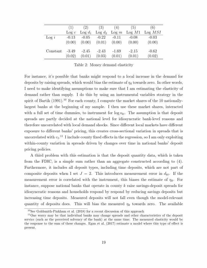
(1) (2) (3) (4) (5) (6)Log c Log d1 Log d2 Log m Log M1 Log MSI

Log i -0.13 -0.05 -0.22 -0.11 -0.08 -0.03(0.00) (0.00) (0.01) (0.00) (0.00) (0.00)

Constant -3.49 -2.45 -2.43 -1.69 -2.15 -0.62(0.02) (0.01) (0.03) (0.01) (0.01) (0.02)

Table 2: Money demand elasticity

For instance, it’s possible that banks might respond to a local increase in the demand fordeposits by raising spreads, which would bias the estimate of ηd towards zero. In other words,I need to make identifying assumptions to make sure that I am estimating the elasticity ofdemand rather than supply. I do this by using an instrumental variables strategy in thespirit of Bartik (1991).10 For each county, I compute the market shares of the 10 nationally-largest banks at the beginning of my sample. I then use these market shares, interactedwith a full set of time dummies, to instrument for log skt. The assumption is that depositspreads are partly decided at the national level for idiosyncratic bank-level reasons andtherefore uncorrelated with local demand shocks. Since different local markets have differentexposure to different banks’ pricing, this creates cross-sectional variation in spreads that isuncorrelated with υt.11 I include county fixed effects in the regression, so I am only exploitingwithin-county variation in spreads driven by changes over time in national banks’ depositpricing policies.

A third problem with this estimation is that the deposit quantity data, which is takenfrom the FDIC, is a simple sum rather than an aggregate constructed according to (4).Furthermore, it includes all deposit types, including time deposits, which are not part ofcomposite deposits when I set J = 2. This introduces measurement error in dkt. If themeasurement error is correlated with the instrument, this biases the estimate of ηd. Forinstance, suppose national banks that operate in county k raise savings-deposit spreads foridiosyncratic reasons and households respond by respond by reducing savings deposits butincreasing time deposits. Measured deposits will not fall even though the model-relevantquantity of deposits does. This will bias the measured ηd towards zero. The available

10See Goldsmith-Pinkham et al. (2018) for a recent discussion of this approach11One worry may be that individual banks may change spreads and other characteristics of the deposit

service (such as the perceived solvency of the bank) at the same time. The measured elasticity would bethe response to the sum of these changes. Egan et al. (2017) estimate a model where this type of effect ispresent.

19

quantity data, which does not distinguish by deposit type, does not make it possible toovercome this possible bias.

The results are shown on Table 3. The estimated elasticity is ηd = 0.20

Log dht(1) (2)OLS IV

Log sht -0.098 -0.200(0.009) (0.004)

Observations 18732 18732

Table 3: Demand for deposits

Using equations (35) and (36), together η = 0.11, ηd = 0.20, γ = 0.76 and cd= 0.22, I

obtain parameter values ε = 0.53 and α = 0.20.Finally, I need to estimate ∂ log s

∂ logN. To do this, I first compute Herfindahl concentration

indices Hkt for each county and time period. I then estimate the following specification,separately for each deposit type:12

sjkt = (ajk + bj logHkt) it + υjkt (41)

where sjkt is the spread on deposit type j in county k in period t and ajk is a vector ofcounty fixed effects. (41) imposes the linearity of spreads in i implied by the model but letsthe slope vary by county and over time within a county if that county’s Herfindahl indexchanges. I then obtain d log s

d logNas follows:

d log s

d logN= −1

s

ds

d logH

= −

(J∑j=1

αjs1−εdj

)−1( J∑j=1

αjs−εdj

dsjd logH

)

= −∑J

j=1 αjγ−εdj bj∑J

j=1 αjγ1−εdj

(42)

The first step just uses that with symmetric banks H = 1N. The second step uses formula

(7) for aggregating spreads on different deposit types. The final step uses that sj = γji and12Estimating (41) instead of a specification with log sjkt on the left hand side avoids having to transform

the data to deal with negative measured spreads.

20

replaces dsjd logH

with its empirical estimate bj.The problem with estimating equation (41) by OLS is that Hkt is likely endogenous.

For instance, a rise in spreads for idiosyncratic county-level reasons (for instance, due to anincrease in county-level deposit demand) could attract bank entry, lowering Hkt. This wouldbias the estimate of bj downwards.

To overcome this, I exploit mergers between large banks as a predictor of concentration.Garmaise and Moskowitz (2006) use a related approach to measure the effect of bank mergerson local social and economic indicators. Following their criteria, I compile a list of all thebank mergers and acquisitions in which both banks had at least $1 billion in assets in the yearprior to the merger. There are a total of 654 valid mergers between 1998 and 2017, the timerange for which I have RateWatch data. For each county, I compute market shares at thebeginning of the sample. I then compute a fictitious time series H̃kt of the Herfindahl indexfor each county by assuming that market shares stay constant except when there are mergers;when two banks that have branches in the same country merge, I add their market shares.I then use log H̃kt as an instrument for logHkt in estimating (41). Since ajk are county fixedeffects, I am only exploiting the within-county variation that comes from changes in localconcentration that are the result of mergers between large banks. The results are shownon Table 4. In the IV specification, both checking and savings spreads are estimated torespond to bank concentration, with similar magnitudes. Applying formula (42) results in ameasured elasticity of spreads with respect to entry of ∂ log s

∂ logN= −1.36.

Log s1 Log s2(1) (2) (3) (4)OLS IV OLS IV

log(HHI)*i −0.029 1.008 −0.027 1.040(0.005) (0.107) (0.007) (0.132)

Observations 40742 40742 40742 40742

Table 4: Spreads and concentration

There have been previous attempts to measure the effect of concentration on depositspreads. Also using RateWatch and FDIC data, Drechsler et al. (2017) find significanteffects of concentration when estimating a first-differences specification, which regresses thechange in spreads on the change in interest rates, interacted with a measure of concentration.For measuring the profit-eroding effect of entry, what matters is the effect on levels ratherthan first-differences (although if spreads are exactly linear functions of interest rates, the

21

two formulations should give the same answer). In Italian data, Focarelli and Panetta (2003)find that mergers tend to raise spreads in the short run but lower them in the long run, buttheir focus is on comparing merged with unmerged banks rather that measuring the effectof concentration on market-wide spreads. Prager and Hannan (1998) find that mergers areassociated with an increase in market-wide spreads. In an older dataset, Berger and Hannan(1989) find a positive association between concentration and savings deposit spreads.

2.4 Welfare measures

Using the measured values of ∂ log s∂ logN

= −1.36, ε = 0.53, η = 0.11, α = 0.20 and ηd = 0.20 informula (29), I obtain

du

di

1

m= −0.32

At a nominal interest rate of 3%, the estimates from Table 2 indicate that m is equal to 34%

of GDP. Therefore the welfare cost of a one percentage point rise in inflation is:

du

GDP=du

di

1

m︸ ︷︷ ︸−0.32

m

GDP︸ ︷︷ ︸0.27

di︸︷︷︸0.01

= 0.084%

or 8.4 basis points of GDP.Table 5 shows how sensitive this magnitude is to various assumptions. As discussed

in Section 2.2, I don’t have the data that would enable me to estimate the elasticity ofsubstitution across deposit types. The baseline figures are computed under the assumptionthat εd = 1 but, as shown in columns 2-4, this makes a relatively minor difference.

As discussed in Section 2.3, there are reasons to believe that the estimation of the elas-ticity of demand for deposits may be biased towards zero. Columns 5 and 6 show the resultsof re-doing the calculations assuming a demand for deposits that is more elastic than thebaseline ηd = 0.20. Higher values of ηd imply a higher welfare cost of inflation. The reasoncan be seen from equation (24). Higher ηd implies that entry responds more strongly tochanges in the interest rate. A more elastic demand for deposits means that when entrylowers spreads, profits fall less because the quantity of deposits increases more. As a result,more entry is needed to restore the free entry condition, so more resources are dedicated tobank fixed costs.

Column 7 shows the effect of re-doing the whole calculation assuming J = 3, with smalltime deposits as a third component of composite deposits. Spreads on time deposits aremuch lower than those on savings accounts but despite being cheaper for households, the

22

quantity held is lower. The model therefore infers that they have little weight in compositedeposits (α3 = 0.1) and including them doesn’t change the figure very much.

Baseline εd = 0.5 εd = 2 εd = 10 ηd = 0.5 ηd = 1 J = 38.4 7.4 9.1 9.8 9.9 15.1 10.1

Table 5: Welfare costs under different assumptions (b.p. of GDP)

Table 6 compares the welfare cost that I find with those obtained by other methods.Perhaps the most common approach is the one by Lucas (2000) and Ireland (2009). Theyassume that the relevant measure of money is M1 (adjusted for retail sweeps), and thatmoney does not pay interest. In this case, using the values for M1 from Table 2, the welfarecost of a one percentage point increase in inflation is:13

du

GDP= − ηM1︸︷︷︸

0.08

M1

GDP︸ ︷︷ ︸0.15

di︸︷︷︸0.01

= 0.012%

Both Lucas (2000) and Ireland (2009) mention that the focus on M1 as the relevantmonetary aggregate is somewhat arbitrary. An alternative, advocated by Cysne (2003), is tobase the calculation on the type of Törnquist-Theil-Divisia monetary aggregate proposed byBarnett (1980). The Monetary Services Index (MSI) and its associated user cost constructedby the Federal Reserve Bank of St. Louis is an example of this (see Anderson and Jones(2011) for details). By definition, the user cost is the opportunity cost of holding one unitof the index. I estimate the slope of this user cost with respect to interest rates (usingspecification (38) to account for possible stickiness) in order to measure how changes in theinterest rate translate into changes in the cost of monetary services, and obtain γMSI = 0.47.Using this value and the demand estimates from Table 2, I obtain the following measure ofthe welfare cost of inflation:

du

GDP= − ηMSI︸ ︷︷ ︸

0.03

MSI

GDP︸ ︷︷ ︸0.6

γMSI︸ ︷︷ ︸0.47

di︸︷︷︸0.01

= 0.022%

13Lucas (2000) estimates a log-log specification like (39) while Ireland (2009) estimates a semi-log specifi-cation logmt = a0 + a1it + υt. This makes a difference for computing the welfare impact of a large changein inflation (both authors focus on the welfare gain of bringing the interest rate all the way down to zero).For a local change of the type considered here, the choice of specification doesn’t make much difference aslong as it’s a good local approximation at the point of interest. The number I find applying this approachis not the same as the actual numbers from Lucas (2000) because he estimates the money-demand elasticityon a different sample and finds a higher number.

23

A similar exercise can be conducted using the model-implied index m instead of the MSI.This is simply the welfare cost of inflation from the model if the entry margin is shut down.Conceptually, the model-implied index m and the MSI are similar, except that the MSI isconstructed on the basis of finer categories and is constructed solely on the basis of pricesand quantities, without relying on estimates of the elasticity of substitution. Nevertheless,using both aggregates yields similar numbers.

I also compute the welfare cost from the model under the assumption that fixed costs donot represent real resource costs but are fees rebated back to the household (but taking intoaccount the spread-reducing effects of entry). This produces an even lower figure than justshutting down the entry margin.

Baseline Using M1 Using the MSI Using m, no bank entry Using m, entry is transfer8.4 1.2 2.2 2.3 1.2

Table 6: Welfare costs under alternative methods (b.p. of GDP)

3 Conclusion

There is very strong evidence that deposit spreads, and thus the profitability of banks, arehigher when interest rates are higher. If the banking industry is characterized by free entryand high fixed costs, this implies that a permanently higher inflation rate will induce realresources to be dedicated to chasing these profits. This is a large component of the welfarecost of inflation.

References

Aiyagari, S. R., Braun, R. A. and Eckstein, Z.: 1998, Transaction services, inflation, andwelfare, Journal of political Economy 106(6), 1274–1301.

Amel, D. F., Kennickell, A. B., Moore, K. B. et al.: 2008, Banking market definition:evidence from the survey of consumer finances. FEDS Working Paper 2008-35.

Amel, D. F. and Starr-McCluer, M.: 2002, Market definition in banking: Recent evidence,The Antitrust Bulletin 47(1), 63–89.

Anderson, R. G. and Jones, B.: 2011, A comprehensive revision of the us monetary services(divisia) indexes, Federal Reserve Bank of St. Louis Review 93(September/October 2011).

24

Bailey, M. J.: 1956, The welfare cost of inflationary finance, Journal of Political Economy64(2), 93–110.

Barnett, W. A.: 1980, Economic monetary aggregates - an application of index number andaggregation theory, Journal of Econometrics 14, 11–48.

Bartik, T. J.: 1991, Who benefits from state and local economic development policies?

Berger, A. N. and Hannan, T. H.: 1989, The price-concentration relationship in banking,The Review of Economics and Statistics pp. 291–299.

Bresciani Turroni, C.: 1937, The economics of inflation: A Study of Currency Depreciationin Post-War Germany, George Allen and Unwin, London.

Craig, B. R. and Dinger, V.: 2014, The duration of bank retail interest rates, InternationalJournal of the Economics of Business 21(2), 191–207.

Cysne, R. P.: 2003, Divisia index, inflation, and welfare, Journal of Money, Credit andBanking 35(2), 221–238.

Di Tella, S. and Kurlat, P.: 2017, Why are banks exposed to monetary policy? StanfordUniversity Working Paper.

Dotsey, M. and Ireland, P.: 1996, The welfare cost of inflation in general equilibrium, Journalof Monetary Economics 37(1), 29–47.

Drechsler, I., Savov, A. and Schnabl, P.: 2017, The deposits channel of monetary policy, TheQuarterly Journal of Economics 132(4), 1819–1876.

Driscoll, J. C. and Judson, R.: 2013, Sticky deposit rates. FEDS Working Paper No. 2013-80.

Egan, M., Hortaçsu, A. and Matvos, G.: 2017, Deposit competition and financial fragility:Evidence from the us banking sector, American Economic Review 107(1), 169–216.

English, W. B.: 1999, Inflation and financial sector size, Journal of Monetary Economics44(3), 379 – 400.

Focarelli, D. and Panetta, F.: 2003, Are mergers beneficial to consumers? evidence from themarket for bank deposits, American Economic Review 93(4), 1152–1172.

25

Garmaise, M. J. and Moskowitz, T. J.: 2006, Bank mergers and crime: The real and socialeffects of credit market competition, the Journal of Finance 61(2), 495–538.

Goldsmith-Pinkham, P., Sorkin, I. and Swift, H.: 2018, Bartik instruments: What, when,why, and how. NBER Working Paper.

Hannan, T. H. and Berger, A. N.: 1991, The rigidity of prices: Evidence from the bankingindustry, The American Economic Review 81(4), 938.

Ireland, P. N.: 2009, On the welfare cost of inflation and the recent behavior of moneydemand, American Economic Review 99(3), 1040–52.

Kleiman, E.: 1989, The costs of inflation. Working Paper, Hebrew University of Jerusalem.

Lucas, R. E.: 2000, Inflation and welfare, Econometrica pp. 247–274.

Marom, A.: 1998, Inflation and israel’s banking industry, Bank of Israel Economic Review62, 30–41.

Neumark, D. and Sharpe, S. A.: 1992, Market structure and the nature of price rigidity:evidence from the market for consumer deposits, The Quarterly Journal of Economics107(2), 657–680.

Prager, R. A. and Hannan, T. H.: 1998, Do substantial horizontal mergers generate sig-nificant price effects? evidence from the banking industry, The Journal of IndustrialEconomics 46(4), 433–452.

Wicker, E.: 1986, Terminating hyperinflation in the dismembered habsburg monarchy, TheAmerican Economic Review 76(3), 350–364.

Yankov, V.: 2014, In search of a risk-free asset. FEDS Working Paper No. 2014-108.

Yoshino, J. A.: 1993, Money and banking regulation: The welfare costs of inflation. Ph.D.dissertation, University of Chicago.

26