ARTICLE

Depleted depletion drives polymer swelling in poorsolvent mixturesDebashish Mukherji1, Carlos M. Marques 2, Torsten Stuehn1 & Kurt Kremer1

Establishing a link between macromolecular conformation and microscopic interaction is a

key to understand properties of polymer solutions and for designing technologically relevant

“smart” polymers. Here, polymer solvation in solvent mixtures strike as paradoxical phe-

nomena. For example, when adding polymers to a solvent, such that all particle interactions

are repulsive, polymer chains can collapse due to increased monomer–solvent repulsion. This

depletion induced monomer–monomer attraction is well known from colloidal stability. A

typical example is poly(methyl methacrylate) (PMMA) in water or small alcohols. While

polymer collapse in a single poor solvent is well understood, the observed polymer swelling in

mixtures of two repulsive solvents is surprising. By combining simulations and theoretical

concepts known from polymer physics and colloidal science, we unveil the microscopic,

generic origin of this collapse–swelling–collapse behavior. We show that this phenomenon

naturally emerges at constant pressure when an appropriate balance of entropically driven

depletion interactions is achieved.

DOI: 10.1038/s41467-017-01520-5 OPEN

1Max-Planck Institut für Polymerforschung, Ackermannweg 10, 55128 Mainz, Germany. 2 Institut Charles Sadron, Université de Strasbourg, CNRS, 23 rue duLoess, 67034 Strasbourg Cedex 2, France. Correspondence and requests for materials should be addressed to D.M. (email: mukherji@mpip-mainz.mpg.de)or to K.K. (email: kremer@mpip-mainz.mpg.de)

NATURE COMMUNICATIONS |8: �1374� |DOI: 10.1038/s41467-017-01520-5 |www.nature.com/naturecommunications 1

1234

5678

90

The understanding of coil-to-globule transition of a mac-romolecule in solvent mixtures is a fundamental process forfunctional soft matter with a huge variety of applications

that goes beyond traditional polymer science1, 2. This reaches fromthe responsiveness of hydrogels to external stimuli3, 4 and bio-medical applications5–8 to the processing of conjugated polymersfor organic electronics9. In this context, it has been commonlyobserved that a polymer can collapse in a mixture of twocompeting, well miscible good solvents, while the same polymerremains expanded in these two individual components. Thisphenomenon is commonly known as co-non-solvency2, 10–19.However, it has also been observed that a polymer can becollapsed in two different poor solvents, whereas it is “better”soluble in their mixtures20–23. Thus far a multitude of specific,system-dependent explanations hindered the emergence of a clearphysical picture of these two intriguing phenomena. While thephenomenon of co-non-solvency has been recently brought onto afirmer ground of a generic explanation2, 18, no equivalentunderstanding of the collapse–swelling–collapse behavior has yetbeen achieved.

In a standard poor solvent, starting from a good solventcondition, an increase of the effective attraction between themonomers first brings the polymer into Θ—conditions, where theradius of gyration scales as Rg ! N1=2

l with Nl being the chainlength24, 25. Upon further increase of the attraction, a polymerthen collapses into a globular state. The resultant collapsedglobule can be understood by balancing negative second virialosmotic contributions and three-body repulsions. The effectiveattraction between the monomers of a polymer can be viewed as adepletion induced attraction, a phenomenon well described forcolloidal suspensions26–30 of purely repulsive particles. In thiscontext, monomer attraction will occur when monomer–solventexcluded volume interactions become large enough. The resultingisolated polymer conformation can be well described by thePorod scaling law of the static structure factor S(q)∝ q−4 fol-lowing the envelope of the correlation peaks in S(q), presenting acompact spherical globule. Interestingly, even if a polymer exhi-bits poor solvent conditions in two different solvents, it canpossibly be somewhat swollen by intermediate mixing ratios ofthe two poor solvents. A system that shows thiscollapse–swelling–collapse scenario is poly(methyl methacrylate)(PMMA) in aqueous alcohol mixtures. More specifically, waterand alcohol are “almost” perfectly miscible and individually poorsolvents for PMMA. However, PMMA shows improved solubilitywithin intermediate mixing concentrations of aqueous alcoholand/or other solvent mixtures20–23.

In this work, we propose a microscopic, generic and thus quitegenerally applicable picture of this collapse–swelling–collapsebehavior in poor solvent mixtures. Therefore, we aim to do thefollowing: (1) devise a thermodynamically consistent generic(chemically independent) model such that solubility of manypolymers in mixtures of poor solvents, including PMMA inaqueous alcohol, can be explained within a simplified (universal)physical concept, (2) develop a microscopic understanding of thecollapse–swelling–collapse scenario and show that micro-scopically this is a second order effect, and (3) investigate if apolymer in mixed poor solvents can really reach a fully swollenstate characteristic of good solvents. To achieve the above goals,we combine generic molecular dynamics, all-atom simulationsand analytical theoretical arguments to study polymer behavior inpoor solvent mixtures.

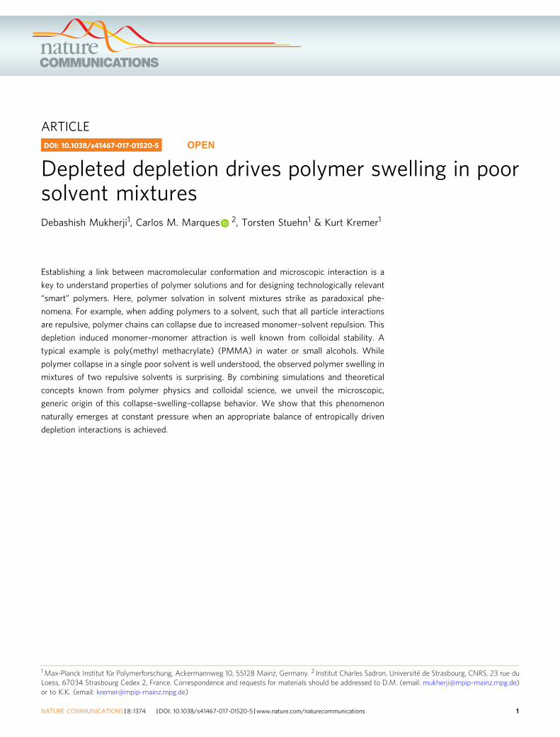
ResultsConformation of polymer. Figure 1 summarizes results for thenormalized squared radius of gyration R2

g ¼ R2g

D E= Rg xc ¼ 0ð Þ2! "

as a function of cosolvent mole fraction xc from the generic modeland for three different cases described in the SupplementaryTable 1. A closer look at the symmetric case of two almost per-fectly miscible, but otherwise identical solvents (black Δ) showsthat—while the pure solvent (xc= 0) and the pure cosolvent (xc=1) are equally poor solvents for the polymer, the same polymerswells within the intermediate cosolvent compositions, reaching amaximum swelling of R2

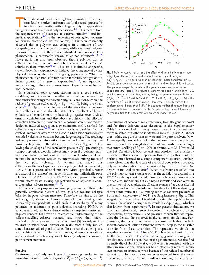
g by ~20% at around xc= 0.5. How couldthis be? Certainly, if both solvent and cosolvent were perfectlymiscible, nothing should happen in this case, as this would benothing but identical to a single component solution. Further-more, given that this is a case of standard poor solvent collapse,polymer conformations are determined by depletion forces (ordepletion induced attraction)28. When cosolvents are added intothe polymer–solvent system (such as the addition of alcohol in aPMMA–water system), the addition of cosolvents not only repels(or depletes) monomers, but also repels solvents and vice versa. Inthis context, if we analyze the all-atom system of aqueous alcoholmixtures, we find that the total number density of the system ρtotalshows a minimum at 50/50 mixing ratios at constant pressure of1 atm and temperature of 300 K, see Supplementary Fig. 1. Thissuggests that, when alcohol is added in water, the repulsive forcesbetween the solution components result in a dip in ρtotal, which isalso known from experiments31. In our generic simulations, wetune solvent–solvent, solvent–cosolvent, cosolvent–cosolventinteractions, temperature T and pressure P such that we repro-duce the density dip observed in the all-atom simulations. Fur-thermore, the system parameters are chosen such that the bulksolvent–cosolvent solution mixture remains deep in the misciblestate far from phase separation. The representative simulationsnapshot is shown in Fig. 2 for a 50/50 solvent–cosolvent mixture.In the main panel of Fig. 2, we show ρtotal used in our genericsimulations. It can be seen that, in the generic model, we also finda density dip of about 10% at xc= 0.5, which is consistent with theall-atom simulations. This leads to an effectively reduced repul-sive interaction around xc= 0.5 because of the reduced number ofsolvent particles near the monomer as expected from the varia-tion of ρtotal with xc. The net result is a swelling of the polymer

1.7Symmetric

Case 1Case 2

R2 g

1.6

1.5

1.4

1.3

1.2

1.1

1.0

0.0 0.2 0.4 0.6xc

0.8 1.0

Fig. 1 Polymer conformation and the effect of different mixtures of poorsolvent conditions. Normalized squared radius of gyration R

2g ¼

R2gD E

= Rg xc ¼ 0ð Þ2D E

as a function of cosolvent molar concentration xc.Results are shown for the generic simulations and for three different cases.The parameter-specific details of the generic cases are listed in theSupplementary Table 1. The results are shown for a chain length of Nl= 30,which corresponds to ! 30‘p with ‘p being the persistence length. HereRg xc ¼ 0ð Þ2

D E= 2.6± 0.4σ2 and R

2Θ ¼ 2:13 with RΘ ¼ RΘ=Rg xc ¼ 0ð Þ is the

normalized Θ—point gyration radius. Here case 2 closely mimics theconformational behavior of PMMA in aqueous methanol mixture based onthe parameterization presented in the Supplementary Table 1. Lines arepolynomial fits to the data that are drawn to guide the eye

ARTICLE NATURE COMMUNICATIONS | DOI: 10.1038/s41467-017-01520-5

2 NATURE COMMUNICATIONS |8: �1374� |DOI: 10.1038/s41467-017-01520-5 |www.nature.com/naturecommunications

chain around xc= 0.5. We coin here the term depleted depletionfor explaining the reduction of depletion forces responsible forpolymer collapse due to mutual solvent–cosolvent exclusion.Notice, however, that this is a common concept in colloidal sci-ence, where the modifications of the depletion attraction profiledue to depletant-depletant interactions have been extensivelystudied28–30.

When the interaction asymmetry between polymer-cosolventεpc and polymer–solvent εps is increased (Supplementary Table 1),where εpc for case 2< case 1< symmetric case, not only thedegree of swelling increases, but the swelling region also shiftsbetween 0.5< xc< 0.9. This range is found to be in excellentagreement with the experimental observation of PMMA con-formations in aqueous alcohol mixtures21, 22. Specifically, ourcase 2 closely resembles PMMA in an aqueous methanol mixture.Indeed, we tune our monomer–solvent and monomer–cosolventinteractions in the generic model such that we can reproduce thecorrect solvation free energy, as measured by the shift in excesschemical potential per monomer μp, known from all-atomsimulations of a PMMA system in aqueous methanol mixtures(Supplementary Fig. 4 and Supplementary Note 2). Furthermore,because we reproduce μp and ρtotal variation with changing xc inour generic model as known from all-atom simulations underambient condition, T= 0.5ε/kB in the generic model correspondsto 300 K and P= 16.0ε/σ3 corresponds to 1 atm in all-atomsystem. While the swelling around xc ! 50%, especially for thesymmetric case, is bulk solution number density dependent (atconstant pressure), the shift in the region of maximal swelling iscosolvent–monomer interaction dependent. For example,cosolvent–monomer repulsion for symmetric case> case 1> case2. This is similar to the PMMA solvation in different aqueousalcohol mixtures, where the repulsion of methanol–MMA>ethanol–MMA> propanol–MMA20–23.

Single-chain structure factor. A closer look at Fig. 1 shows thatthe degree of swelling, within the range 0.5< xc< 0.9, variesbetween 20 and 65% (or 10 and 30% in Rg), depending on theinteraction assymetry. Considering that we are dealing withcombinations of poor solvents, this is a very significant swelling,making PMMA-based materials permeable to water–alcoholmixtures. Moreover, analyzing the simulations, it becomesapparent that the polymer does not necessarily reach a fully

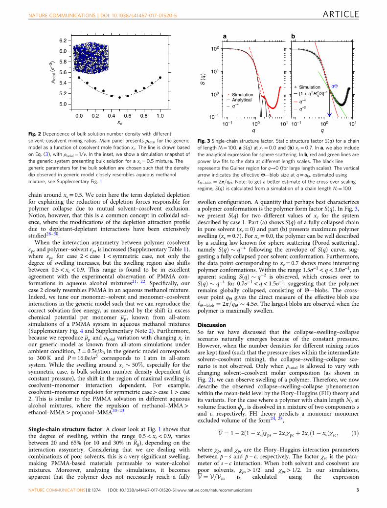
swollen configuration. A quantity that perhaps best characterizesa polymer conformation is the polymer form factor S(q). In Fig. 3,we present S(q) for two different values of xc for the systemdescribed by case 1. Part (a) shows S(q) of a fully collapsed chainin pure solvent (xc= 0) and part (b) presents maximum polymerswelling (xc= 0.7). For xc= 0.0, the polymer can be well describedby a scaling law known for sphere scattering (Porod scattering),namely SðqÞ ! q%4 following the envelope of S(q) curve, sug-gesting a fully collapsed poor solvent conformation. Furthermore,the data point corresponding to xc= 0.7 shows more interestingpolymer conformations. Within the range 1.5σ−1< q< 3.0σ−1, anaparent scaling SðqÞ ! q%2 is observed, which crosses over toSðqÞ ! q%4 for 0.7σ−1< q< 1.5σ−1, suggesting that the polymerremains globally collapsed, consisting of Θ—blobs. The cross-over point qΘ gives the direct measure of the effective blob size‘Θ%blob ¼ 2π=qΘ ! 4:5σ. The largest blobs are observed when thepolymer is maximally swollen.

DiscussionSo far we have discussed that the collapse–swelling–collapsescenario naturally emerges because of the constant pressure.However, when the number densities for different mixing ratiosare kept fixed (such that the pressure rises within the intermediatesolvent–cosolvent mixing), the collapse–swelling–collapse sce-nario is not observed. Only when ρtotal is allowed to vary withchanging solvent–cosolvent molar composition (as shown inFig. 2), we can observe swelling of a polymer. Therefore, we nowdescribe the observed collapse–swelling–collapse phenomenonwithin the mean-field level by the Flory–Huggins (FH) theory andits variants. For the case where a polymer with chain length Nl, atvolume fraction ϕp, is dissolved in a mixture of two components sand c, respectively, FH theory predicts a monomer–monomerexcluded volume of the form24, 25,

V ¼ 1% 2 1% xcð Þχps % 2xcχpc þ 2xc 1% xcð Þχsc; ð1Þ

where χps and χpc are the Flory–Huggins interaction parametersbetween p − s and p − c, respectively. The factor χsc is the para-meter of s − c interaction. When both solvent and cosolvent arepoor solvents, χps> 1/2 and χpc> 1/2. In our simulations,V ¼ V=Vm is calculated using the expression

0.80.60.4xc

0.20.0

6.2

! tot

al ("–3

)6.0

5.8

5.6

5.4

5.2

5.0

1.0

Fig. 2 Dependence of bulk solution number density with differentsolvent–cosolvent mixing ratios. Main panel presents ρtotal for the genericmodel as a function of cosolvent mole fraction xc. The line is drawn basedon Eq. (3), with ρtotal= 1/v. In the inset, we show a simulation snapshot ofthe generic system presenting bulk solution for a xc= 0.5 mixture. Thegeneric parameters for the bulk solution are chosen such that the densitydip observed in generic model closely resembles aqueous methanolmixture, see Supplementary Fig. 1

101 10–1 101100

q–4

qΘ

q–2

102

a b

S (

q) 101

Simulation

Simulation[1 + q 2R 2

g/3]–1

Analyticalq–4

100

10–1

10–1 100

q q

Fig. 3 Single-chain structure factor. Static structure factor S(q) for a chainof length Nl= 100. a S(q) at xc= 0.0 and (b) xc= 0.7. In a, we also includethe analytical expression for sphere scattering. In b, red and green lines arepower law fits to the data at different length scales. The black linerepresents the Guiner region for q→0 (for large length scales). The verticalarrow indicates the effective Θ—blob size at q= qΘ, estimated using‘Θ%blob ¼ 2π=qΘ. Note: to get a better estimate of the cross-over scalingregime, S(q) is calculated from a simulation of a chain length Nl= 100

NATURE COMMUNICATIONS | DOI: 10.1038/s41467-017-01520-5 ARTICLE

NATURE COMMUNICATIONS |8: �1374� |DOI: 10.1038/s41467-017-01520-5 |www.nature.com/naturecommunications 3

V ¼ 2πR

1% e%vðrÞ=kBT# $

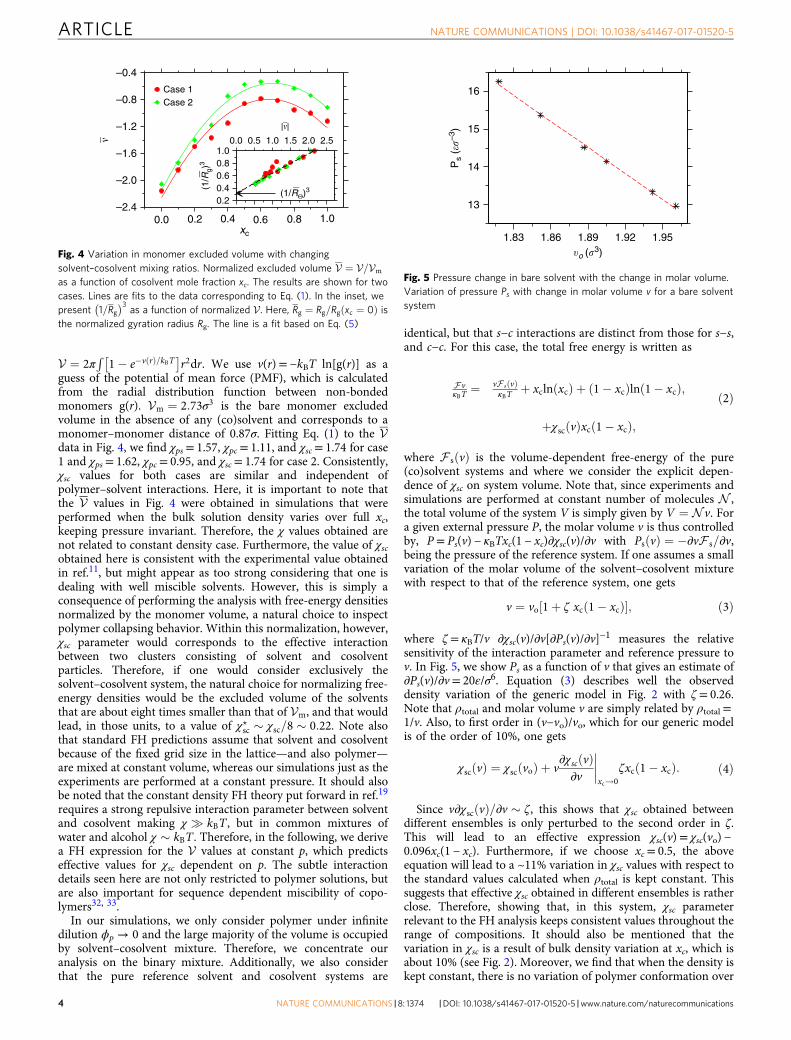
r2dr. We use v(r)= −kBT ln[g(r)] as aguess of the potential of mean force (PMF), which is calculatedfrom the radial distribution function between non-bondedmonomers g(r). Vm ¼ 2:73σ3 is the bare monomer excludedvolume in the absence of any (co)solvent and corresponds to amonomer–monomer distance of 0.87σ. Fitting Eq. (1) to the Vdata in Fig. 4, we find χps= 1.57, χpc= 1.11, and χsc= 1.74 for case1 and χps= 1.62, χpc= 0.95, and χsc= 1.74 for case 2. Consistently,χsc values for both cases are similar and independent ofpolymer–solvent interactions. Here, it is important to note thatthe V values in Fig. 4 were obtained in simulations that wereperformed when the bulk solution density varies over full xc,keeping pressure invariant. Therefore, the χ values obtained arenot related to constant density case. Furthermore, the value of χscobtained here is consistent with the experimental value obtainedin ref.11, but might appear as too strong considering that one isdealing with well miscible solvents. However, this is simply aconsequence of performing the analysis with free-energy densitiesnormalized by the monomer volume, a natural choice to inspectpolymer collapsing behavior. Within this normalization, however,χsc parameter would corresponds to the effective interactionbetween two clusters consisting of solvent and cosolventparticles. Therefore, if one would consider exclusively thesolvent–cosolvent system, the natural choice for normalizing free-energy densities would be the excluded volume of the solventsthat are about eight times smaller than that of Vm, and that wouldlead, in those units, to a value of χ?sc ! χsc=8 ! 0:22. Note alsothat standard FH predictions assume that solvent and cosolventbecause of the fixed grid size in the lattice—and also polymer—are mixed at constant volume, whereas our simulations just as theexperiments are performed at a constant pressure. It should alsobe noted that the constant density FH theory put forward in ref.19

requires a strong repulsive interaction parameter between solventand cosolvent making χ ' kBT , but in common mixtures ofwater and alcohol χ ! kBT . Therefore, in the following, we derivea FH expression for the V values at constant p, which predictseffective values for χsc dependent on p. The subtle interactiondetails seen here are not only restricted to polymer solutions, butare also important for sequence dependent miscibility of copo-lymers32, 33.

In our simulations, we only consider polymer under infinitedilution ϕp → 0 and the large majority of the volume is occupiedby solvent–cosolvent mixture. Therefore, we concentrate ouranalysis on the binary mixture. Additionally, we also considerthat the pure reference solvent and cosolvent systems are

identical, but that s−c interactions are distinct from those for s−s,and c−c. For this case, the total free energy is written as

FvκBT

¼ vF sðvÞκBT

þ xcln xcð Þ þ 1% xcð Þln 1% xcð Þ;

þχscðvÞxc 1% xcð Þ;

ð2Þ

where F sðvÞ is the volume-dependent free-energy of the pure(co)solvent systems and where we consider the explicit depen-dence of χsc on system volume. Note that, since experiments andsimulations are performed at constant number of molecules N ,the total volume of the system V is simply given by V ¼ N v. Fora given external pressure P, the molar volume v is thus controlledby, P= Ps(v) − κBTxc(1 − xc)∂χsc(v)/∂v with PsðvÞ ¼ %∂vF s=∂v,being the pressure of the reference system. If one assumes a smallvariation of the molar volume of the solvent–cosolvent mixturewith respect to that of the reference system, one gets

v ¼ vo 1þ ζ xcð1% xcÞ½ ); ð3Þ

where ζ= κBT/v ∂χsc(v)/∂v[∂Ps(v)/∂v]−1 measures the relativesensitivity of the interaction parameter and reference pressure tov. In Fig. 5, we show Ps as a function of v that gives an estimate of∂Ps(v)/∂v= 20ε/σ6. Equation (3) describes well the observeddensity variation of the generic model in Fig. 2 with ζ= 0.26.Note that ρtotal and molar volume v are simply related by ρtotal=1/v. Also, to first order in (v−vo)/vo, which for our generic modelis of the order of 10%, one gets

χscðvÞ ¼ χsc voð Þ þ v∂χscðvÞ∂v

%%%%xc!0

ζxc 1% xcð Þ: ð4Þ

Since v∂χscðvÞ=∂v ! ζ, this shows that χsc obtained betweendifferent ensembles is only perturbed to the second order in ζ.This will lead to an effective expression χsc(v)= χsc(vo) −0.096xc(1 − xc). Furthermore, if we choose xc= 0.5, the aboveequation will lead to a ~11% variation in χsc values with respect tothe standard values calculated when ρtotal is kept constant. Thissuggests that effective χsc obtained in different ensembles is ratherclose. Therefore, showing that, in this system, χsc parameterrelevant to the FH analysis keeps consistent values throughout therange of compositions. It should also be mentioned that thevariation in χsc is a result of bulk density variation at xc, which isabout 10% (see Fig. 2). Moreover, we find that when the density iskept constant, there is no variation of polymer conformation over

0.0

–0.4

Case 1Case 2–0.8

–1.2

–1.6

#

–2.0

–2.40.2 0.4 0.6

xc

0.8 1.0

(1/RΘ)3(1/R

g)3

1.00.80.60.40.2

0.0 0.5 1.0

|#|1.5 2.0 2.5

Fig. 4 Variation in monomer excluded volume with changingsolvent–cosolvent mixing ratios. Normalized excluded volume V ¼ V=Vm

as a function of cosolvent mole fraction xc. The results are shown for twocases. Lines are fits to the data corresponding to Eq. (1). In the inset, wepresent 1=Rg

& '3as a function of normalized V. Here, Rg ¼ Rg=Rg xc ¼ 0ð Þ is

the normalized gyration radius Rg. The line is a fit based on Eq. (5)

1.951.921.891.86$o ("

3)1.83

16

Ps

(%"–3

) 15

14

13

Fig. 5 Pressure change in bare solvent with the change in molar volume.Variation of pressure Ps with change in molar volume v for a bare solventsystem

ARTICLE NATURE COMMUNICATIONS | DOI: 10.1038/s41467-017-01520-5

4 NATURE COMMUNICATIONS |8: �1374� |DOI: 10.1038/s41467-017-01520-5 |www.nature.com/naturecommunications

full xc range, while pressure of the system goes up with a max-imum at xc= 0.5.

Our numerical predictions successfully account for polymerswelling in solutions of poor solvent mixtures, as the simulationsquantitatively demonstrate. While this fascinating polymerbehavior is driven by purely repulsive interactions, it also revealsthe subtle balance of depletion forces and bulk solution propertiesthat enable such a paradoxical phenomenon. Indeed, polymercollapse in repulsive solvents can be understood by depletioninduced attractions28. The dominant contribution to depletioninduced attraction originates from direct monomer–solventrepulsion, and is thus proportional to solvent number densityρtotat dictating the number of depletants. When a few solventmolecules are replaced by cosolvents, for example, a water by analcohol, this preserves the solvent density to the first order. Underthese conditions, one smoothly interpolates between two polymercollapsed states, without any swelling at intermediate composi-tions. Here, however, interactions between solvent componentsplay a delicate role in dictating the depletion forces by bringing incontributions proportional to second (or to even higher)-ordercontributions of ρtotat, see Fig. 2. Interestingly, it is well knownfrom colloidal sciences that such second order effects may reducecolloid–colloid attractive forces29, 30. Moreover, these studies incolloidal systems typically deal with two component systemswhere size asymmetry of 10 is needed to observe higher ordereffects. In our study, size asymmetry between monomer andsolvent is significantly smaller and second order effects originatebecause of the peculiar properties of the solvent–cosolvent mix-tures. Thus, the polymer case occurs in a different interactionregime compared to colloidal effect. The solvent–cosolventexcluded volume is slightly stronger than the correspondingvalues for solvent–solvent and cosolvent–cosolvent molecules,leading to a slightly smaller solution density and a correspondingdiminution of the effective depletion interaction. At intermediatecompositions, where solvent–cosolvent interactions are dominantin the solution, the effect is the strongest. Therefore, a broadvariety of polymer/solvent systems are expected to display such abehavior.

A standard measure of the attractive forces leading to polymercollapse is provided by the monomer excluded volume V. Forpoor solvents, V is negative and the dimensions of the chain canbe understood by balancing the second (negative) virial osmoticcontributions and the three body repulsion24, 25, leading to

R3Θ

R3g

% 1 ¼ V%% %%: ð5Þ

In the inset of Fig. 4, we show 1=Rg& '3 as a function of V,

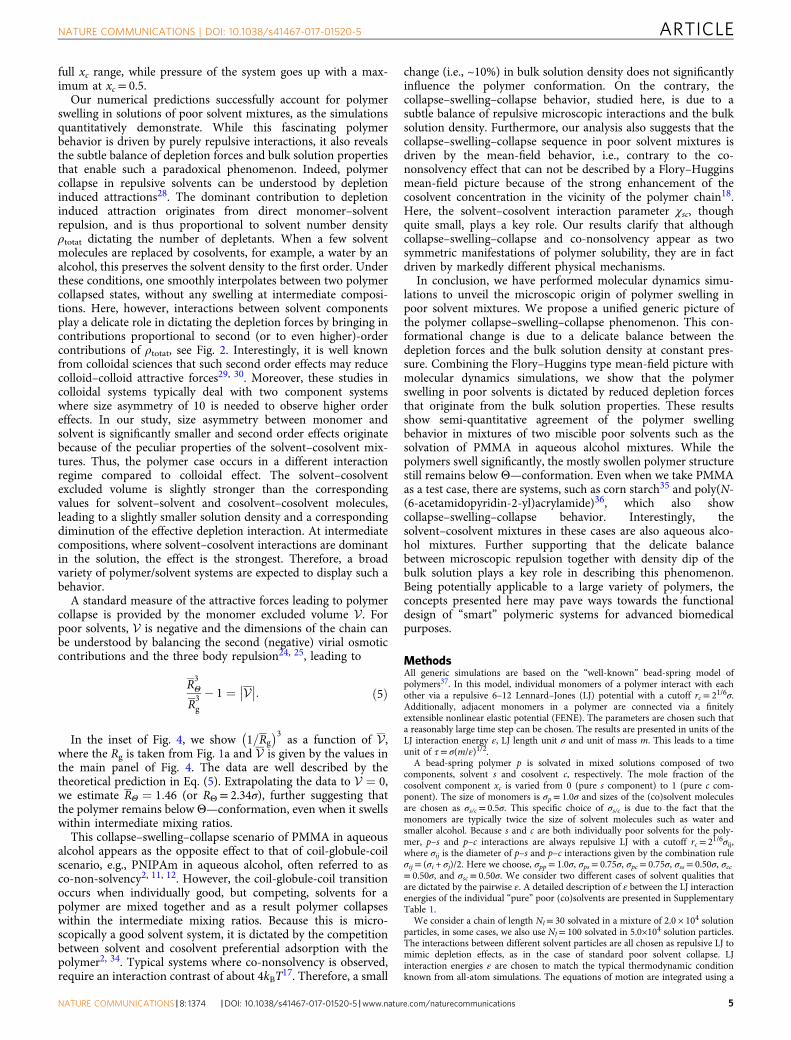
where the Rg is taken from Fig. 1a and V is given by the values inthe main panel of Fig. 4. The data are well described by thetheoretical prediction in Eq. (5). Extrapolating the data to V ¼ 0,we estimate RΘ ¼ 1:46 (or RΘ= 2.34σ), further suggesting thatthe polymer remains below Θ—conformation, even when it swellswithin intermediate mixing ratios.

This collapse–swelling–collapse scenario of PMMA in aqueousalcohol appears as the opposite effect to that of coil-globule-coilscenario, e.g., PNIPAm in aqueous alcohol, often referred to asco-non-solvency2, 11, 12. However, the coil-globule-coil transitionoccurs when individually good, but competing, solvents for apolymer are mixed together and as a result polymer collapseswithin the intermediate mixing ratios. Because this is micro-scopically a good solvent system, it is dictated by the competitionbetween solvent and cosolvent preferential adsorption with thepolymer2, 34. Typical systems where co-nonsolvency is observed,require an interaction contrast of about 4kBT17. Therefore, a small

change (i.e., ~10%) in bulk solution density does not significantlyinfluence the polymer conformation. On the contrary, thecollapse–swelling–collapse behavior, studied here, is due to asubtle balance of repulsive microscopic interactions and the bulksolution density. Furthermore, our analysis also suggests that thecollapse–swelling–collapse sequence in poor solvent mixtures isdriven by the mean-field behavior, i.e., contrary to the co-nonsolvency effect that can not be described by a Flory–Hugginsmean-field picture because of the strong enhancement of thecosolvent concentration in the vicinity of the polymer chain18.Here, the solvent–cosolvent interaction parameter χsc, thoughquite small, plays a key role. Our results clarify that althoughcollapse–swelling–collapse and co-nonsolvency appear as twosymmetric manifestations of polymer solubility, they are in factdriven by markedly different physical mechanisms.

In conclusion, we have performed molecular dynamics simu-lations to unveil the microscopic origin of polymer swelling inpoor solvent mixtures. We propose a unified generic picture ofthe polymer collapse–swelling–collapse phenomenon. This con-formational change is due to a delicate balance between thedepletion forces and the bulk solution density at constant pres-sure. Combining the Flory–Huggins type mean-field picture withmolecular dynamics simulations, we show that the polymerswelling in poor solvents is dictated by reduced depletion forcesthat originate from the bulk solution properties. These resultsshow semi-quantitative agreement of the polymer swellingbehavior in mixtures of two miscible poor solvents such as thesolvation of PMMA in aqueous alcohol mixtures. While thepolymers swell significantly, the mostly swollen polymer structurestill remains below Θ—conformation. Even when we take PMMAas a test case, there are systems, such as corn starch35 and poly(N-(6-acetamidopyridin-2-yl)acrylamide)36, which also showcollapse–swelling–collapse behavior. Interestingly, thesolvent–cosolvent mixtures in these cases are also aqueous alco-hol mixtures. Further supporting that the delicate balancebetween microscopic repulsion together with density dip of thebulk solution plays a key role in describing this phenomenon.Being potentially applicable to a large variety of polymers, theconcepts presented here may pave ways towards the functionaldesign of “smart” polymeric systems for advanced biomedicalpurposes.

MethodsAll generic simulations are based on the “well-known” bead-spring model ofpolymers37. In this model, individual monomers of a polymer interact with eachother via a repulsive 6–12 Lennard–Jones (LJ) potential with a cutoff rc= 21/6σ.Additionally, adjacent monomers in a polymer are connected via a finitelyextensible nonlinear elastic potential (FENE). The parameters are chosen such thata reasonably large time step can be chosen. The results are presented in units of theLJ interaction energy ε, LJ length unit σ and unit of mass m. This leads to a timeunit of τ= σ(m/ε)1/2.

A bead-spring polymer p is solvated in mixed solutions composed of twocomponents, solvent s and cosolvent c, respectively. The mole fraction of thecosolvent component xc is varied from 0 (pure s component) to 1 (pure c com-ponent). The size of monomers is σp= 1.0σ and sizes of the (co)solvent moleculesare chosen as σs/c= 0.5σ. This specific choice of σs/c is due to the fact that themonomers are typically twice the size of solvent molecules such as water andsmaller alcohol. Because s and c are both individually poor solvents for the poly-mer, p–s and p–c interactions are always repulsive LJ with a cutoff rc= 21/6σij,where σij is the diameter of p–s and p–c interactions given by the combination ruleσij= (σi + σj)/2. Here we choose, σpp= 1.0σ, σps= 0.75σ, σpc= 0.75σ, σss= 0.50σ, σcc= 0.50σ, and σsc= 0.50σ. We consider two different cases of solvent qualities thatare dictated by the pairwise ε. A detailed description of ε between the LJ interactionenergies of the individual “pure” poor (co)solvents are presented in SupplementaryTable 1.

We consider a chain of length Nl= 30 solvated in a mixture of 2.0 × 104 solutionparticles, in some cases, we also use Nl= 100 solvated in 5.0×104 solution particles.The interactions between different solvent particles are all chosen as repulsive LJ tomimic depletion effects, as in the case of standard poor solvent collapse. LJinteraction energies ε are chosen to match the typical thermodynamic conditionknown from all-atom simulations. The equations of motion are integrated using a

NATURE COMMUNICATIONS | DOI: 10.1038/s41467-017-01520-5 ARTICLE

NATURE COMMUNICATIONS |8: �1374� |DOI: 10.1038/s41467-017-01520-5 |www.nature.com/naturecommunications 5

velocity Verlet algorithm with a time step δt= 0.01τ. The simulations were usuallyequilibrated for 107 MD time steps. The measurements are typically observed overanother 106 MD steps. During this time, observables such as the gyration radius Rg,static structure factor S(q), chemical potential of polymer μp, and the polymerexcluded volume V is calculated. The temperature is set to 0.5ε/kBT, which isemployed using a Langevin thermostat with damping constant γ= 1.0τ−1.

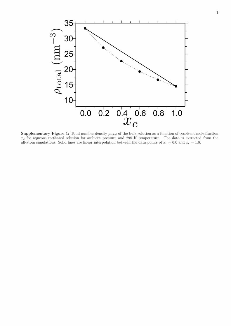
One of the most important aspects of modeling PMMA in aqueous alcohol is toincorporate bulk solution properties. As mentioned earlier in the main manuscripttext, alcohol and water are poor solvents for PMMA, while it swells inwater–alcohol mixtures. Analyzing the experimental data31 and all-atom simula-tions of aqueous alcohol mixtures, it has become apparent that the excess volumeof the mixtures increases (or decrease in the total solution number density ρtotal)from the mean-field values, which follows in a nonlinear dependence with xc(Supplementary Fig. 1). This deviation is most dominant at intermediate mixingratios. In our generic simulation protocol, we choose interaction parameters of thesolution components such that ρtotal of the solution decreases at around 50–50mixture, while keeping the solution at constant pressure. For this purpose, wechoose εss= εcc= 0.5 and εsc= 2.5, keeping all the interactions repulsive (Supple-mentary Table 1). It is important to mention that ρtotal= 5.5σ−3 for pure xc= 0 andxc= 1 solutions. This corresponds to a pressure of p≈ 16.0± 0.5ε/σ3. The advan-tage of this choice of ρtotal is that the solution remains stable over full xc range,when the ρtotal decreases by ≈10% at xc= 0.5.

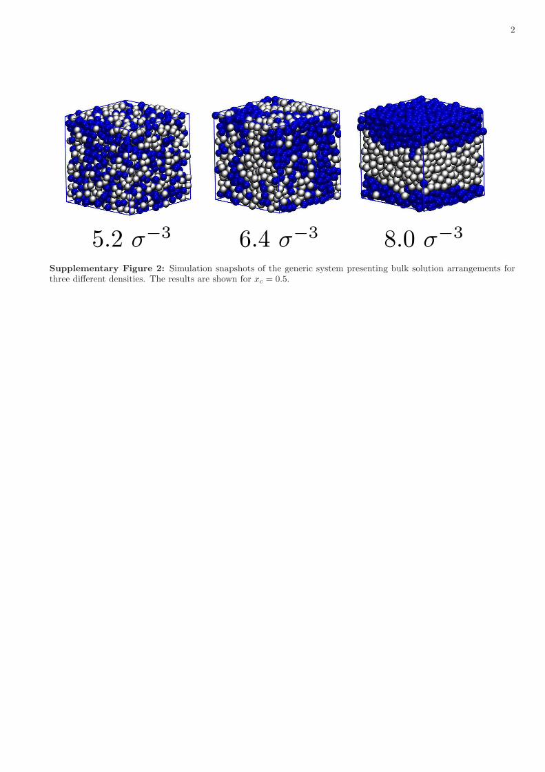
We also want to mention that even when the parameters are chosen as repulsivewith c−s being more repulsive than c−c and s−s interaction, our bulk solutionremains homogeneous over the full range of mixing ratios. In this context, it isimportant to note that the solution phase separation is intimately linked to thesolution density. Within our choice of ρtotal, we do not see any phase separation. InSupplementary Fig. 2, we show three simulation snapshots for different ρtotal andfor xc= 0.5. It can be appreciated that there is no signature of phase separationwhen ρtotal= 5.2σ−3, phase separation can only be seen for ρtotal 6:4σ

%3. Suggestingthat the bulk solution remains stable. Furthermore, to quantify the possibility ofany phase separation we calculate the quantity η defined as,

η ¼ Vss þ Vcc % 2Vsc: ð6Þ

Here V ij is the excluded volume of the i−j interaction defined as,

V ij ¼ 2πZ 1

01% e%vijðrÞ=κBTh i

r2dr; ð7Þ

where vij is the potential of mean force between i and j components. We findη ¼ %0:4σ3 for ρtotal= 5.2σ−3, η= −5.5σ3 for ρtotal= 6.4σ−3, and η< −30.0σ3 forρtotal= 8.0σ−3. It can be appreciated that η→0 for ρtotal → 5.2σ−3, further suggestingthat the bulk solution is stable.

The details about generic simulations and all-atom force field parameters aregiven in the electronic Supplementary Material. Generic simulations are performedusing the ESPResSo + +molecular dynamics package38, all-atom simulations areperformed using the GROMACS package39, and simulation snapshots are renderedusing VMD40.

Data availability. All presented and analyzed the data is included in both maintext and in the Supplementary Material, including the methods, force fields, andtheory developed. Generic simulation scripts will be made available through theESPResSo++ webpage http://www.espresso-pp.de/.

Received: 28 February 2017 Accepted: 25 September 2017

References1. Cohen-Stuart, M. A. et al. Emerging applications of stimuli-responsive polymer

materials. Nat. Mater. 9, 101 (2010).2. Mukherji, D., Marques, C. M. & Kremer, K. Polymer collapse in miscible good

solvents is a generic phenomenon driven by preferential adsorption. Nat.Commun. 5, 4882 (2014).

3. Chang, D. P., Dolbow, J. E. & Zauscher, S. Switchable friction of stimulus-responsive hydrogels. Langmuir 23, 250 (2007).

4. Schmidt, S. et al. Adhesion and mechanical properties of PNIPAM microgelfilms and their potential use as switchable cell culture substrates. Adv. Funct.Mater. 20, 3235 (2010).

5. Vogel, M. J. & Steen, P. H. Capillarity-based switchable adhesion. Proc. NatlAcad. Sci. USA 107, 3377 (2010).

6. Lee, H., Lee, B. P. & Messersmith, P. B. A reversible wet/dry adhesive inspiredby mussels and geckos. Nature 448, 338 (2007).

7. Meddahi-Pelle, A. et al. Organ repair, hemostasis, and in vivo bonding ofmedical devices by aqueous solutions of nanoparticles. Angew. Chem., Int. Ed.53, 6369 (2014).

8. de Beer, S., Kutnyanszky, E., Schön, P. M., Vansco, G. J. & Müser, M. H. Solventinduced immiscibility of polymer brushes eliminates dissipation channels. Nat.Commun. 5, 3781 (2014).

9. Hernandez-Sosa, G. et al. Rheological and drying considerations for uniformlygravure-printed layers: towards large-area flexible organic light-emitting diodes.Adv. Funct. Mat. 23, 3164 (2013).

10. Wolf, B. A. & Willms, M. M. Measured and calculated solubility of polymers inmixed solvents: Co-nonsolvency. Makromol. Chem. 179, 2265 (1978).

11. Schild, H. G., Muthukumar, M. & Tirrell, D. A. Cononsolvency in mixedaqueous solutions of poly(N-isopropylacrylamide). Macromolecules 24, 948(1991).

12. Zhang, G. & Wu, C. Reentrant coil-to-globule-to-coil transition of a singlelinear homopolymer chain in a water/methanol mixture. Phys. Rev. Lett. 86,822 (2001).

13. Hiroki, A., Maekawa, Y., Yoshida, M., Kubota, K. & Katakai, R. Volume phasetransitions of poly(acryloyl-L-proline methyl ester) gels in response to water-alcohol composition. Polymer 42, 1863 (2001).

14. Kiritoshi, K. & Ishihara, K. EMolecular recognition of alcohol by volume phasetransition of cross-linked poly(2-methacryloyloxyethyl phosphorylcholine) gel.Sci. Technol. Adv. Mater. 4, 93 (2003).

15. Lund, R., Willner, L., Stellbrink, J., Radulescu, A. & Richter, D. Role ofinterfacial tension for the structure of PEP-PEO polymeric micelles. Acombined SANS and pendant drop tensiometry investigation. Macromolecules37, 9984 (2004).

16. Heyda, J., Muzdalo, A. & Dzubiella, J. Rationalizing polymer swelling andcollapse under attractive cosolvent conditions. Macromolecules 46, 1231 (2013).

17. Mukherji, D. & Kremer, K. Coil-globule-coil transition of PNIPAm in aqueousmethanol: Coupling all-atom simulations to semi-grand canonical coarse-grained reservoir. Macromolecules 46, 9158 (2013).

18. Mukherji, D., Marques, C. M., Stuehn, T. & Kremer, K. Co-non-solvency:Mean-field polymer theory does not describe polymer collapse transition in amixture of two competing good solvents. J. Chem. Phys. 142, 114903 (2015).

19. Dudowicz, J., Freed, K. F. & Douglas, J. F. Communication: cosolvency andcononsolvency explained in terms of a Flory-Huggins type theory. J. Chem.Phys. 143, 131101 (2015).

20. Masegosa, R. M., Prolongo, M. G., Hernandez-Feures, I. & Horta, A.Preferential and total sorption of poly(methyl methacrylate) in the cosolventsformed by acetonitrile with pentyl acetate and with alcohols (1-butanol, 1-propanol, and methanol). Macromolecules 17, 1181 (1984).

21. Hoogenboom, R., Remzi Becer, C., Guerrero-Sanchez, C., Hoeppener, S. &Schubert, U. S. Solubility and thermoresponsiveness of PMMA in alcohol-watersolvent mixtures. Aust. J. Chem. 63, 1173 (2010).

22. Lee, S. M. & Bae, Y. C. Enhanced solvation effect of re-collapsing behavior forcross-linked PMMA particle gel in aqueous alcohol solutions. Polymer= 55,4684 (2014).

23. Yu, Y., Kieviet, B. D., Kutnyanszky, E., Vancso, G. J. & de Beer, S. Cosolvency-induced switching of the adhesion between Poly(methyl methacrylate) brushes.ACS Macro Lett. 4, 75 (2015).

24. de Gennes, P.-G. Scaling Concepts in Polymer Physics. (Cornell University Press,London, 1979).

25. Des Cloizeaux, J. & Jannink, G. Polymers in Solution: Their Modelling andStructure. (Clarendon Press, Oxford, 1990).

26. Crocker, J. C., Matteo, J. A., Dinsmore, A. D. & Yodh, A. G. Entropic attractionand repulsion in binary colloids probed with a line optical tweezer. Phys. Rev.Lett. 82, 4352 (1999).

27. Phillips, R. et al. Physical Biology of the Cell, 2nd edn (Garland Science 2012).28. Lekkerkerker, H. N. W. & Tuinier, R. Colloids and the Depletion Interaction.

(Clarendon Press, Oxford, 1990).29. Mao, Y., Cates, M. E. & Lekkerkerker, H. N. W. Depletion stabilization by

semidilute rods. Phys. Rev. Lett. 75, 4548 (1995).30. Mao, Y., Cates, M. E. & Lekkerkerker, H. N. W. Depletion force in colloidal

systems. Physica. A 222, 10 (1995).31. Perera, A., Sokolic, F., Almasy, L. & Koga, Y. Kirkwood-Buff integrals of

aqueous alcohol binary mixtures. J. Chem. Phys. 124, 124515 (2006).32. Balazs, A. C., Sanchez, I. C., Epstein, I. R., Karasz, F. E. & MacKnight, W. J.

Effect of sequence distribution on the miscibility of polymer/copolymer blends.Macromolecules 18, 2188 (1985).

33. Balazs, A. C., Karasz, F. E., MacKnight, W. J., Ueda, H. & Sanchez, I. C.Copolymer/copolymer blends: effect of sequence distribution on miscibility.Macromolecules 18, 2784 (1985).

34. Mukherji, D. et al. Relating side chain organization of PNIPAm with itsconformation in aqueous methanol. Soft Matter 12, 7995 (2016).

35. Galvez, L. O., de Beer, S., van der Meer, D. & Pons, A. Dramatic effect of fluidchemistry on cornstarch suspensions: linking particle interactions tomacroscopic rheology. Phys. Rev. E 95, 030602 (2017).

36. Asadujjaman, A., Ahmadi, V., Yalcin, M., ten Brummelhuis, N. & Bertin, A.Thermoresponsive functional polymers based on 2,6-diaminopyridine motif

ARTICLE NATURE COMMUNICATIONS | DOI: 10.1038/s41467-017-01520-5

6 NATURE COMMUNICATIONS |8: �1374� |DOI: 10.1038/s41467-017-01520-5 |www.nature.com/naturecommunications

with tunable UCST behaviour in water/alcohol mixtures. Pol. Chem 8, 3140(2017).

37. Kremer, K. & Grest, G. S. Dynamics of entangled linear polymer melts:amoleculardynamics simulation. J. Chem. Phys. 92, 5057 (1990).

38. Halverson, J. D. et al. ESPResSo++: a modern multiscale simulation package forsoft matter systems. Comp. Phys. Comm. 184, 1129 (2013).

39. Hess, B., Kutzner, C., van der Spoel, D. & Lindahl, E. GROMACS 4: algorithmsfor highly efficient, load-balanced, and scalable molecular simulation. J. Chem.Theory Comput. 4, 435 (2008).

40. Humphrey, W., Dalke, A. & Schulten, K. VMD: visual molecular dynamics. J.Mol. Graph. 14, 33 (1996).

AcknowledgementsD.M. thanks Burkhard Dünweg and Vagelis Harmandaris for many stimulating dis-cussions, Tiago Oliveira for the help to build the all-atom PMMA force field and BjörnBaumeier for suggesting ref.1. in Supplementary Material. C.M.M. acknowledges Max-Planck Institut für Polymerforschung for hospitality where this work was initiated andperformed. We thank Nancy Carolina Forero-Martinez and Hsiao-Ping Hsu for criticalreading of the manuscript.

Author contributionsD.M., C.M.M. and K.K. designed the research and parameterized the model, D.M. andT.S. performed the simulations, D.M., C.M.M. and K.K. analyzed the data and for-mulated the theory and D.M., C.M.M. and K.K. wrote the paper.

Additional informationSupplementary Information accompanies this paper at doi:10.1038/s41467-017-01520-5.

Competing interests: The authors declare no competing financial interests.

Reprints and permission information is available online at http://npg.nature.com/reprintsandpermissions/

Publisher's note: Springer Nature remains neutral with regard to jurisdictional claims inpublished maps and institutional affiliations.

Open Access This article is licensed under a Creative CommonsAttribution 4.0 International License, which permits use, sharing,

adaptation, distribution and reproduction in any medium or format, as long as you giveappropriate credit to the original author(s) and the source, provide a link to the CreativeCommons license, and indicate if changes were made. The images or other third partymaterial in this article are included in the article’s Creative Commons license, unlessindicated otherwise in a credit line to the material. If material is not included in thearticle’s Creative Commons license and your intended use is not permitted by statutoryregulation or exceeds the permitted use, you will need to obtain permission directly fromthe copyright holder. To view a copy of this license, visit http://creativecommons.org/licenses/by/4.0/.

© The Author(s) 2017

NATURE COMMUNICATIONS | DOI: 10.1038/s41467-017-01520-5 ARTICLE

NATURE COMMUNICATIONS |8: �1374� |DOI: 10.1038/s41467-017-01520-5 |www.nature.com/naturecommunications 7

1

0.0 0.2 0.4 0.6 0.8 1.010

15

20

25

30

35

Supplementary Figure 1: Total number density ρtotal of the bulk solution as a function of cosolvent mole fractionxc for aqueous methanol solution for ambient pressure and 298 K temperature. The data is extracted from theall-atom simulations. Solid lines are linear interpolation between the data points of xc = 0.0 and xc = 1.0.

2

Supplementary Figure 2: Simulation snapshots of the generic system presenting bulk solution arrangements forthree different densities. The results are shown for xc = 0.5.

3

0.0 0.2 0.4 0.6 0.8 1.00.8

1.0

1.2

1.4

1.6

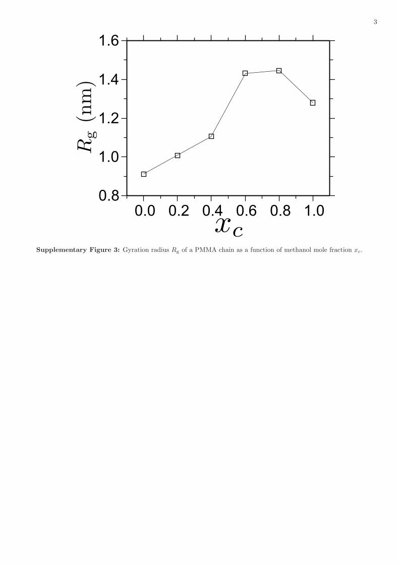
Supplementary Figure 3: Gyration radius Rg of a PMMA chain as a function of methanol mole fraction xc.

4

0.0 0.2 0.4 0.6 0.8 1.0-4.0-3.0-2.0-1.00.0

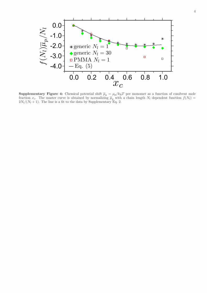
Supplementary Figure 4: Chemical potential shift µp = µp/kBT per monomer as a function of cosolvent molefraction xc. The master curve is obtained by normalizing µp with a chain length Nl dependent function f(Nl) =2Nl/(Nl + 1). The line is a fit to the data by Supplementary Eq. 2.

5

Supplementary Table 1: Lennard-Jones (LJ) interactions for the generic model. p, s and c represents polymer,solvent and cosolvent, respectively.

LJ energy Symmetric Case 1 Case 2 Cut-off

ϵpp 1.0ϵ 1.0ϵ 1.0ϵ 21/6σ

ϵps 3.5ϵ 3.5ϵ 3.5ϵ 0.75× 21/6σ

ϵpc 3.5ϵ 2.5ϵ 2.0ϵ 0.75× 21/6σ

6

Supplementary Note 1: Computational details

In this work a modified OPLS force field of methyl acetate [1] was used to simulate PMMA. We use the SPC/Ewater model [2] and OPLS force field for methanol [3]. A more detailed analysis of the all-atom force field will bepresented elsewhere [4].The temperature is set to 300 K using a Berendsen thermostat with a coupling constant 0.1 ps. The time step for

the simulations is chosen as 1 fs. To obtain equilibrium solvent density, initial configurations are equilibrated for 5 nsusing a Berendsen barostat [5] with a coupling time of 0.5 ps and 1 atm pressure. The production runs are performedin canonical ensemble. The electrostatics are treated using Particle Mesh Ewald [6]. The interaction cutoff is chosenas 1.4 nm.We use PMMA chains of lengths Nl = 30 solvated in a simulation box consisting of 2.0 × 104 solvent molecules

with varying xc. In Supplementary Fig. we show a plot of the all-atom simulation of PMMA in aqueous methanol.We also want to point out that the case 2 in the generic model is tuned to reproduce PMMA solvation in aqueousmethanol. However, the all-atom chain consists of ∼ 15ℓp with ℓp being the presistance length of the chain, while inthe generic model we have simulated a chain of 30ℓp length. If we now take Rg for the maximally swollen chain Rg

and normalized it by (Nl/ℓp)1/3 taking a collapsed chain, we find Rg (Nl/ℓp)

−1/3 = 0.67σ for the generic model and0.59 nm for all-atom chain. This gives a conversion of 1σ ∼ 0.9nm between all-atom and generic simulation.

7

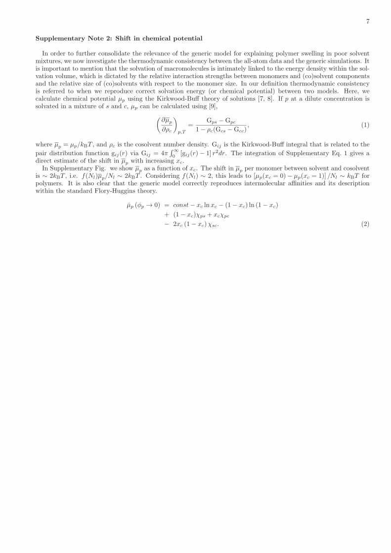
Supplementary Note 2: Shift in chemical potential

In order to further consolidate the relevance of the generic model for explaining polymer swelling in poor solventmixtures, we now investigate the thermodynamic consistency between the all-atom data and the generic simulations. Itis important to mention that the solvation of macromolecules is intimately linked to the energy density within the sol-vation volume, which is dictated by the relative interaction strengths between monomers and (co)solvent componentsand the relative size of (co)solvents with respect to the monomer size. In our definition thermodynamic consistencyis referred to when we reproduce correct solvation energy (or chemical potential) between two models. Here, wecalculate chemical potential µp using the Kirkwood-Buff theory of solutions [7, 8]. If p at a dilute concentration issolvated in a mixture of s and c, µp can be calculated using [9],

(

∂µp

∂ρc

)

p,T

=Gps −Gpc

1− ρc(Gcs −Gcc), (1)

where µp = µp/kBT , and ρc is the cosolvent number density. Gij is the Kirkwood-Buff integral that is related to the

pair distribution function gij(r) via Gij = 4π∫

∞

0[gij(r)− 1] r2dr. The integration of Supplementary Eq. 1 gives a

direct estimate of the shift in µp with increasing xc.In Supplementary Fig. we show µp as a function of xc. The shift in µp per monomer between solvent and cosolvent

is ∼ 2kBT , i.e. f(Nl)µp/Nl ∼ 2kBT . Considering f(Nl) ∼ 2, this leads to [µp(xc = 0)− µp(xc = 1)] /Nl ∼ kBT forpolymers. It is also clear that the generic model correctly reproduces intermolecular affinities and its descriptionwithin the standard Flory-Huggins theory.

µp (φp → 0) = const− xc lnxc − (1− xc) ln (1− xc)

+ (1− xc)χps + xcχpc

− 2xc (1− xc)χsc. (2)

8

[1] K. Murzyn, M. Bratek, and M. Pasenkiewicz-Gierula J. Phys. Chem. B 117, 16388 (2013).[2] H. J. C. Berendsen, J. R. Grigera, and T. P. Straatsma, J. Phys. Chem. 91, 6269 (1987).[3] W. L. Jorgensen, D. S. Maxwell, and J. Tirado-Rives, J. Am. Chem. Soc. 118, 11225 (1996).[4] D. Mukherji, B. Baumeier, and K. Kremer, in preparation.[5] H. J. C. Berendsen, J. P. M. Postma, W. F. van Gunsteren, A. DiNola, and J. R. Haak, J. Chem. Phys. 81, 3684 (1984).[6] U. Essmann, L. Perera, M. L. Berkowitz, T. Darden, H. Lee, L. G. A. Pedersen, J. Chem. Phys. 103 8577 (1995).[7] J. G. Kirkwood and F. P. Buff, J. Chem. Phys. 19, 774 (1951).[8] A. Ben-Naim, J. Phys. Chem. 71, 4002 (1967).[9] J. Rosgen, B. M. Pettitt, and D. W. Bolen, Biophys. J 89, 2988 (2005).