Embed Size (px)
Citation preview

Department of Physics and AstronomyUniversity of Heidelberg
Diploma Thesis in Physics2010
submitted byRebecca Bollborn in Hagen


A Monolithic Active Pixel Sensoras Direct Monitor for
Therapeutic Antiproton and Ion Beams
This diploma thesis has been carried out by
Rebecca Boll
at the
Max-Planck-Institute for Nuclear Physics in Heidelberg
under the supervision of
Prof. Joachim Ullrich
Heidelberg, December 1, 2010

A Monolithic Active Pixel Sensor as Direct Monitor for Therapeutic Antiprotonand Ion Beams
The Mimotera, a monolithic active pixel sensor (MAPS) of crystalline silicon hasbeen investigated regarding its ability to directly monitor antiproton and ion beams,and has been implemented as a beam monitor at the Antiproton Cell Experiment(ACE) at the European Organization for Nuclear Research (CERN). It has beenproven to be a well-suited device for monitoring a spill of about 3 × 10⁷ antipro-tons only 500 ns long, on a shot-to-shot basis in real time without saturating. Thecommissioning of the Mimotera at ACE represents a major improvement, ensuringnot only a more reliable data analysis due to exact profile measurements, but alsospeeding up the initial preparation of the experiment significantly.
Moreover, it has been shown that the Mimotera behaves linearly as a function ofintensity, as well as of the energy loss of a carbon ion beam at the Heidelberg Ion-Beam Therapy Center (HIT). The readout rate of the system is high enough totrack fluctuations in the beam intensity during one spill, such that the Mimoteracould also serve as a tool for fast and reliable quality assurance in hadron therapyfacilities.
Ein monolitischer, aktiver Pixelsensor als direkter Monitor für Antiprotonen-und Ionenstrahlen
Der Mimotera Detektor, ein monolithischer, aktiver Pixelsensor aus kristallinemSilizium wurde hinsichtlich seiner Eignung als direkter Monitor für Antiprotonen-und Ionenstrahlen untersucht. Er wurde im Antiproton Cell Experiment (ACE) ander Europäischen Organisation für Kernforschung (CERN) als Strahlmonitor instal-liert und es wurde gezeigt, dass der Mimotera geeignet ist, einzelne Antiprotonen-schüsse von nur 500 ns Länge und einer Intensität von etwa 3× 10⁷ Teilchen abzu-bilden, ohne dabei in Sättigung zu gehen. Dies bietet eine erhebliche Verbesserungfür ACE, da der Detektor nicht nur eine verlässlichere Datenanalyse durch genaueProfilmessungen ermöglicht, sondern außerdem auch das Einstellen des Strahls zuBeginn des Experimentes deutlich beschleunigt.
Weiterhin wurde gezeigt, dass der Mimotera sich linear als Funktion der Intensitätund des Energieverlustes eines Kohlenstoffionenstrahls am Heidelberger Ionenstrahl-Therapiezentrum (HIT) verhält. Die Ausleserate des Systems ist hoch genug, um einVerfolgen der Intensitätsfluktuationen in jedem einzelnen Spill zu ermöglichen. Da-her ist der Mimotera ein vielversprechendes Instrument, um die Qualitätssicherungin Hadronentherapiezentren zu verbessern.


Contents
1 Motivation 11.1 Development of Hadron Therapy for Cancer Treatment . . . . . . . . 11.2 The Antiproton Cell Experiment . . . . . . . . . . . . . . . . . . . . 61.3 Goal of this Thesis . . . . . . . . . . . . . . . . . . . . . . . . . . . . 8
2 Comparison of Beam Monitoring Systems 92.1 Previously Used Systems at ACE . . . . . . . . . . . . . . . . . . . . 92.2 Semiconductor Radiation Detectors . . . . . . . . . . . . . . . . . . . 11
2.2.1 Basic Functionality . . . . . . . . . . . . . . . . . . . . . . . . 112.2.2 Different Types of Silicon Detectors . . . . . . . . . . . . . . . 15
3 The Mimotera 193.1 Architecture of the Sensor . . . . . . . . . . . . . . . . . . . . . . . . 193.2 Data Acquisition . . . . . . . . . . . . . . . . . . . . . . . . . . . . . 213.3 Data Analysis . . . . . . . . . . . . . . . . . . . . . . . . . . . . . . . 243.4 Why the Mimotera is the System of Choice . . . . . . . . . . . . . . . 27
4 Antiproton Beam at ACE 314.1 The Challenge of Saturation . . . . . . . . . . . . . . . . . . . . . . . 314.2 Beam Monitoring . . . . . . . . . . . . . . . . . . . . . . . . . . . . . 384.3 The Mimotera as an Alignment Tool . . . . . . . . . . . . . . . . . . 41
5 Ion Beams at HIT 435.1 Experimental Conditions at HIT . . . . . . . . . . . . . . . . . . . . . 435.2 Carbon Ions . . . . . . . . . . . . . . . . . . . . . . . . . . . . . . . . 455.3 Protons . . . . . . . . . . . . . . . . . . . . . . . . . . . . . . . . . . 50
6 Open Questions and Summary 536.1 Radiation Damage . . . . . . . . . . . . . . . . . . . . . . . . . . . . 536.2 Summary and Outlook . . . . . . . . . . . . . . . . . . . . . . . . . . 57
A Mimotera Manual for ACE 61A.1 Setting up the system . . . . . . . . . . . . . . . . . . . . . . . . . . . 61A.2 Taking Data . . . . . . . . . . . . . . . . . . . . . . . . . . . . . . . . 63
B Bibliography 69

1 Motivation
1.1 Development of Hadron Therapy for CancerTreatment
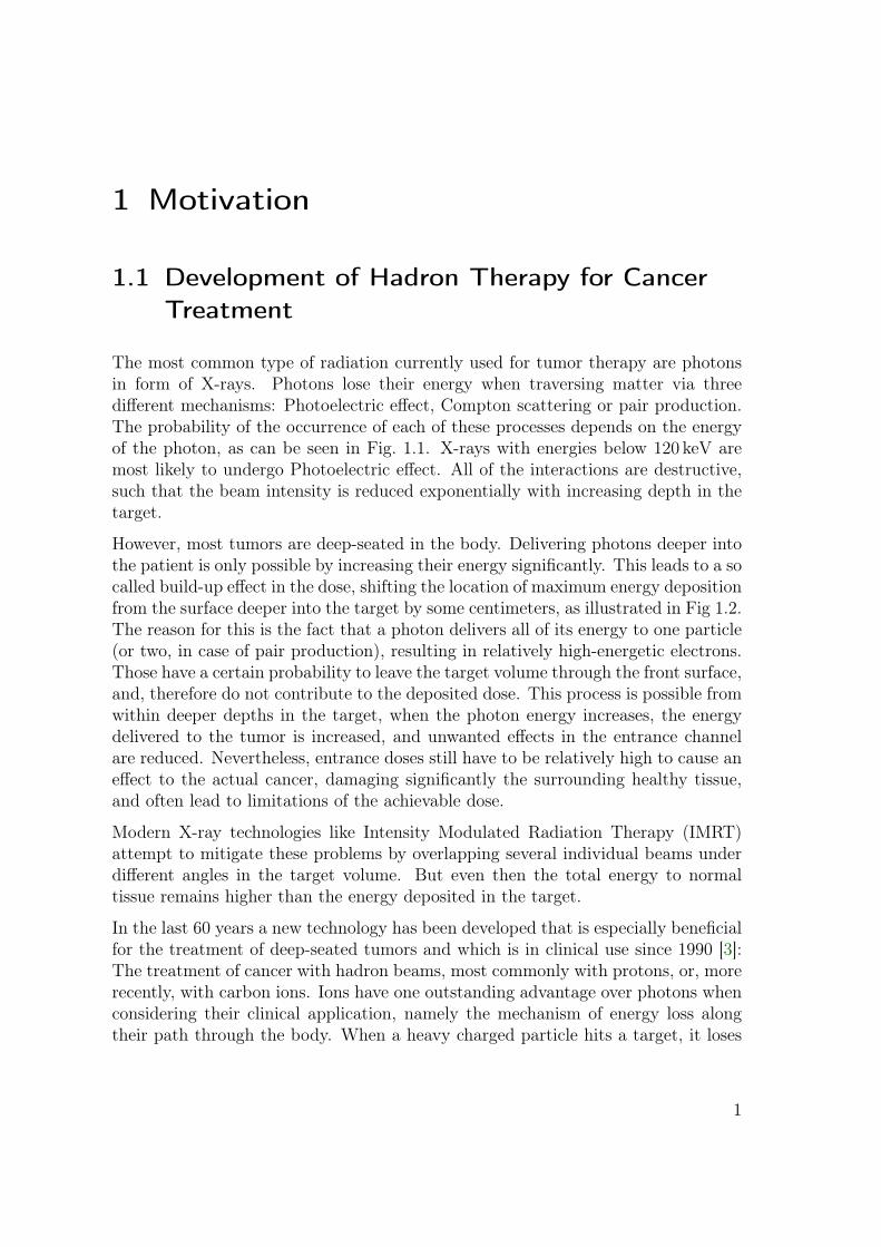
The most common type of radiation currently used for tumor therapy are photonsin form of X-rays. Photons lose their energy when traversing matter via threedifferent mechanisms: Photoelectric effect, Compton scattering or pair production.The probability of the occurrence of each of these processes depends on the energyof the photon, as can be seen in Fig. 1.1. X-rays with energies below 120 keV aremost likely to undergo Photoelectric effect. All of the interactions are destructive,such that the beam intensity is reduced exponentially with increasing depth in thetarget.
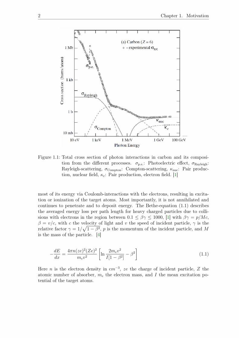
However, most tumors are deep-seated in the body. Delivering photons deeper intothe patient is only possible by increasing their energy significantly. This leads to a socalled build-up effect in the dose, shifting the location of maximum energy depositionfrom the surface deeper into the target by some centimeters, as illustrated in Fig 1.2.The reason for this is the fact that a photon delivers all of its energy to one particle(or two, in case of pair production), resulting in relatively high-energetic electrons.Those have a certain probability to leave the target volume through the front surface,and, therefore do not contribute to the deposited dose. This process is possible fromwithin deeper depths in the target, when the photon energy increases, the energydelivered to the tumor is increased, and unwanted effects in the entrance channelare reduced. Nevertheless, entrance doses still have to be relatively high to cause aneffect to the actual cancer, damaging significantly the surrounding healthy tissue,and often lead to limitations of the achievable dose.
Modern X-ray technologies like Intensity Modulated Radiation Therapy (IMRT)attempt to mitigate these problems by overlapping several individual beams underdifferent angles in the target volume. But even then the total energy to normaltissue remains higher than the energy deposited in the target.
In the last 60 years a new technology has been developed that is especially beneficialfor the treatment of deep-seated tumors and which is in clinical use since 1990 [3]:The treatment of cancer with hadron beams, most commonly with protons, or, morerecently, with carbon ions. Ions have one outstanding advantage over photons whenconsidering their clinical application, namely the mechanism of energy loss alongtheir path through the body. When a heavy charged particle hits a target, it loses
1
2 Chapter 1. Motivation
Figure 1.1: Total cross section of photon interactions in carbon and its composi-tion from the different processes. σp.e.: Photoelectric effect, σRayleigh:Rayleigh-scattering, σCompton: Compton-scattering, κnuc: Pair produc-tion, nuclear field, κe: Pair production, electron field. [1]
most of its energy via Coulomb-interactions with the electrons, resulting in excita-tion or ionization of the target atoms. Most importantly, it is not annihilated andcontinues to penetrate and to deposit energy. The Bethe-equation (1.1) describesthe averaged energy loss per path length for heavy charged particles due to colli-sions with electrons in the region between 0.1 ≤ βγ ≤ 1000, [1] with βγ = p/Mc,β = v/c, with c the velocity of light and v the speed of incident particle, γ is therelative factor γ = 1/
√1− β2, p is the momentum of the incident particle, and M
is the mass of the particle. [4]
−dEdx
=4πn(ze)2(Ze)2
mev2
[ln
2mev2
I[1− β2]− β2
](1.1)
Here n is the electron density in cm−3, ze the charge of incident particle, Z theatomic number of absorber, me the electron mass, and I the mean excitation po-tential of the target atoms.
1.1. Development of Hadron Therapy for Cancer Treatment 3
Figure 1.2: Depth dose curves of photons and carbon ions of different energies inwater. [2]
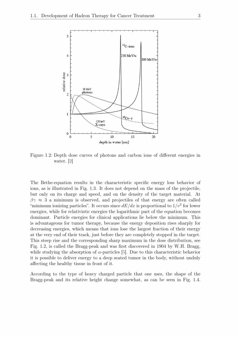
The Bethe-equation results in the characteristic specific energy loss behavior ofions, as is illustrated in Fig. 1.3. It does not depend on the mass of the projectile,but only on its charge and speed, and on the density of the target material. Atβγ ≈ 3 a minimum is observed, and projectiles of that energy are often called“minimum ionizing particles”. It occurs since dE/dx is proportional to 1/v2 for lowerenergies, while for relativistic energies the logarithmic part of the equation becomesdominant. Particle energies for clinical applications lie below the minimum. Thisis advantageous for tumor therapy, because the energy deposition rises sharply fordecreasing energies, which means that ions lose the largest fraction of their energyat the very end of their track, just before they are completely stopped in the target.This steep rise and the corresponding sharp maximum in the dose distribution, seeFig. 1.2, is called the Bragg-peak and was first discovered in 1904 by W.H. Bragg,while studying the absorption of α-particles [5]. Due to this characteristic behaviorit is possible to deliver energy to a deep seated tumor in the body, without undulyaffecting the healthy tissue in front of it.
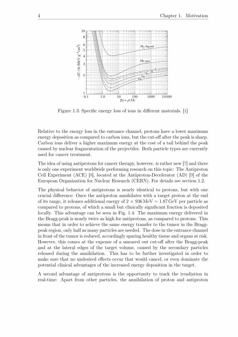
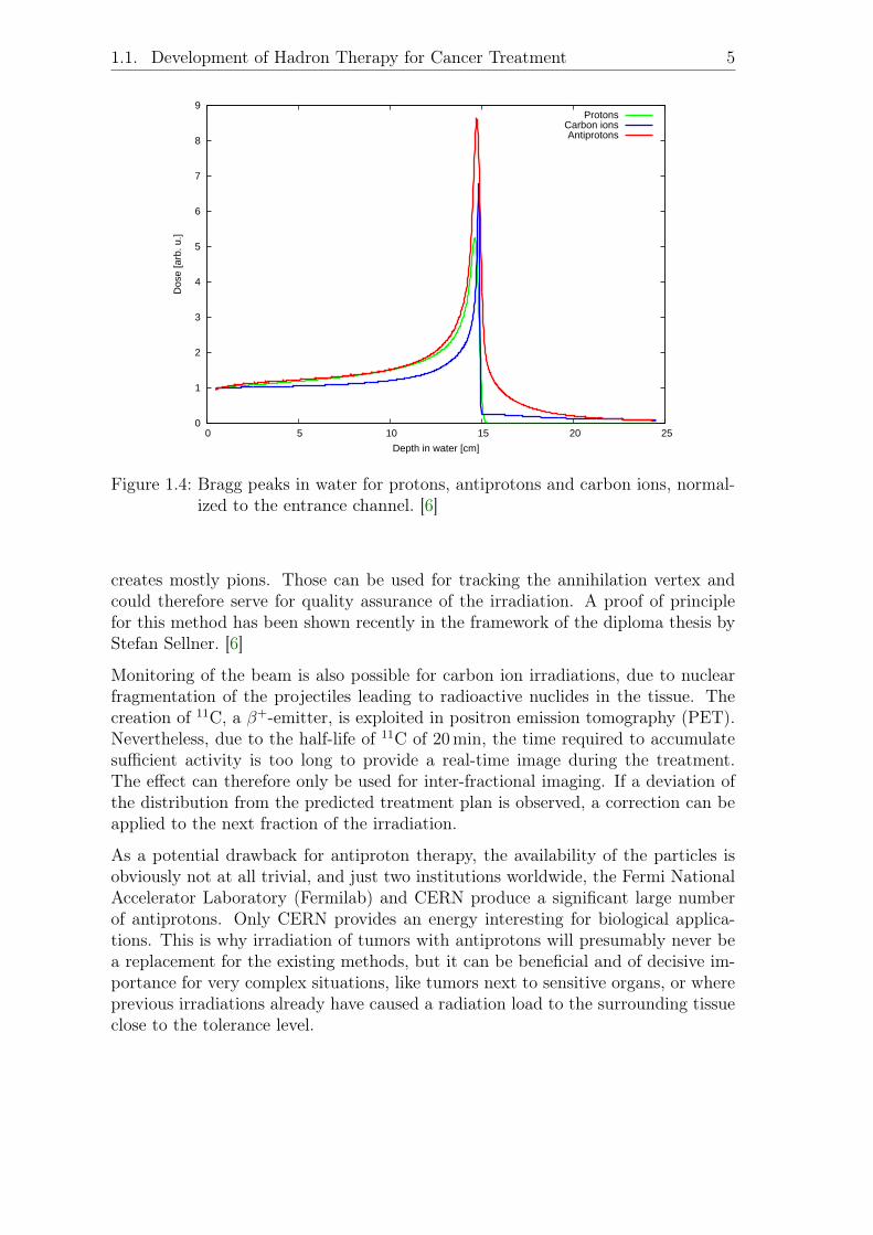
According to the type of heavy charged particle that one uses, the shape of theBragg-peak and its relative height change somewhat, as can be seen in Fig. 1.4.
4 Chapter 1. Motivation
Figure 1.3: Specific energy loss of ions in different materials. [1]
Relative to the energy loss in the entrance channel, protons have a lower maximumenergy deposition as compared to carbon ions, but the cut-off after the peak is sharp.Carbon ions deliver a higher maximum energy at the cost of a tail behind the peakcaused by nuclear fragmentation of the projectiles. Both particle types are currentlyused for cancer treatment.
The idea of using antiprotons for cancer therapy, however, is rather new [7] and thereis only one experiment worldwide performing research on this topic: The AntiprotonCell Experiment (ACE) [8], located at the Antiproton-Decelerator (AD) [9] of theEuropean Organization for Nuclear Research (CERN). For details see section 1.2.
The physical behavior of antiprotons is nearly identical to protons, but with onecrucial difference: Once the antiproton annihilates with a target proton at the endof its range, it releases additional energy of 2 × 936 MeV = 1.87 GeV per particle ascompared to protons, of which a small but clinically significant fraction is depositedlocally. This advantage can be seen in Fig. 1.4: The maximum energy delivered inthe Bragg-peak is nearly twice as high for antiprotons, as compared to protons. Thismeans that in order to achieve the same energy transfer to the tumor in the Bragg-peak region, only half as many particles are needed. The dose in the entrance channelin front of the tumor is reduced, accordingly sparing healthy tissue and organs at risk.However, this comes at the expense of a smeared out cut-off after the Bragg-peakand at the lateral edges of the target volume, caused by the secondary particlesreleased during the annihilation. This has to be further investigated in order tomake sure that no undesired effects occur that would cancel, or even dominate thepotential clinical advantages of the increased energy deposition in the target.
A second advantage of antiprotons is the opportunity to track the irradiation inreal-time: Apart from other particles, the annihilation of proton and antiproton
1.1. Development of Hadron Therapy for Cancer Treatment 5
0
1
2
3
4
5
6
7
8
9
0 5 10 15 20 25
Dos
e [a
rb. u
.]
Depth in water [cm]
ProtonsCarbon ionsAntiprotons
Figure 1.4: Bragg peaks in water for protons, antiprotons and carbon ions, normal-ized to the entrance channel. [6]
creates mostly pions. Those can be used for tracking the annihilation vertex andcould therefore serve for quality assurance of the irradiation. A proof of principlefor this method has been shown recently in the framework of the diploma thesis byStefan Sellner. [6]
Monitoring of the beam is also possible for carbon ion irradiations, due to nuclearfragmentation of the projectiles leading to radioactive nuclides in the tissue. Thecreation of 11C, a β+-emitter, is exploited in positron emission tomography (PET).Nevertheless, due to the half-life of 11C of 20 min, the time required to accumulatesufficient activity is too long to provide a real-time image during the treatment.The effect can therefore only be used for inter-fractional imaging. If a deviation ofthe distribution from the predicted treatment plan is observed, a correction can beapplied to the next fraction of the irradiation.
As a potential drawback for antiproton therapy, the availability of the particles isobviously not at all trivial, and just two institutions worldwide, the Fermi NationalAccelerator Laboratory (Fermilab) and CERN produce a significant large numberof antiprotons. Only CERN provides an energy interesting for biological applica-tions. This is why irradiation of tumors with antiprotons will presumably never bea replacement for the existing methods, but it can be beneficial and of decisive im-portance for very complex situations, like tumors next to sensitive organs, or whereprevious irradiations already have caused a radiation load to the surrounding tissueclose to the tolerance level.

6 Chapter 1. Motivation
1.2 The Antiproton Cell Experiment
Figure 1.5: CERN accelerator complex.
The Antiproton Cell Experiment is dedicated to investigations of an innovativeapproach for cancer therapy. It is located at the Antiproton Decelerator (AD) atCERN, see Fig. 1.5. The antiprotons are produced by shooting 26 GeV/c protonscoming from the Proton Synchrotron on an Iridium target. The maximum yield ofantiprotons produced in this collision lies around 3.6 GeV/c, and antiprotons in anarrow band around this momentum are captured by a magnetic horn and injectedinto the Antiproton Decelerator. They are decelerated and cooled in several steps.Once a kinetic energy of 126 MeV (502 MeV/c momentum) is reached, they areejected to ACE. Usually the antiprotons are decelerated to 5 MeV (100 MeV/c) andare sent to the three main experiments operating at the AD, studying antihydrogen.
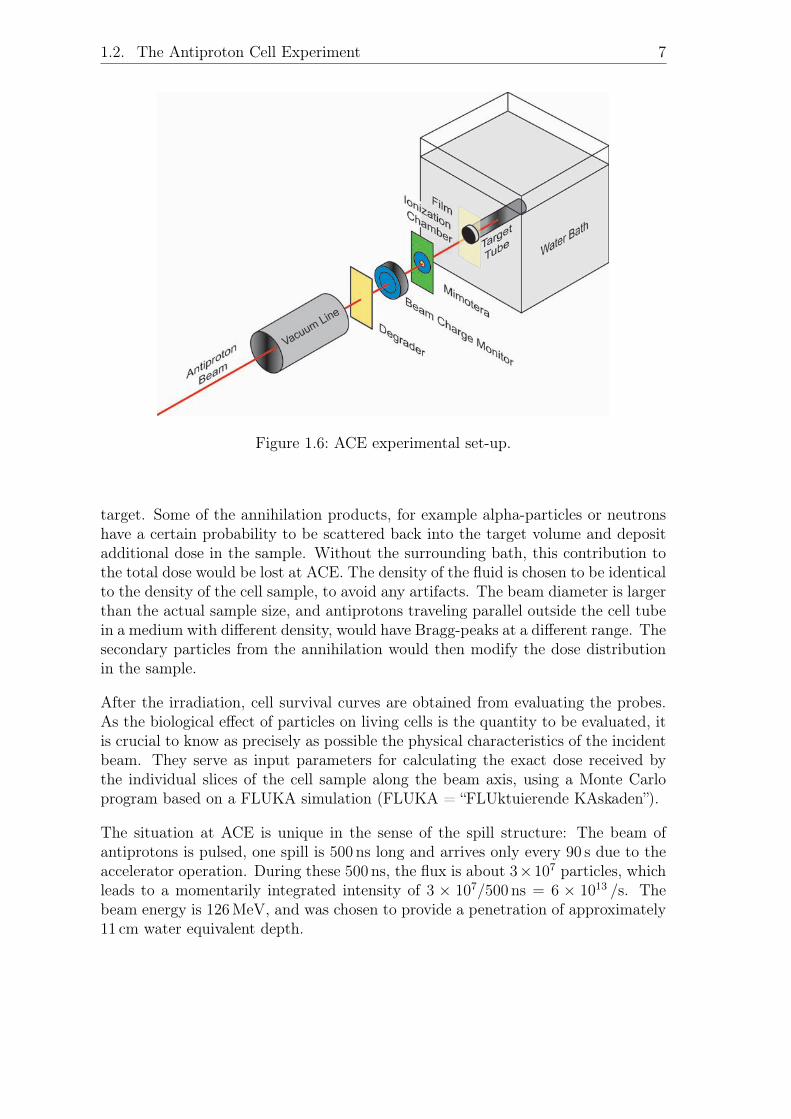
The experimental set-up is displayed in Fig. 1.6: The antiproton beam enters aPMMA tank; in its center, along the central beam axis, PMMA tubes filled withV79-WNRE Chinese Hamster cells embedded into gelatin are placed. The usage ofthese special cells allows correlations to experiments with other radiation modalities,because they are used worldwide in a variety of different clinical tests. [10] The beamenergy can be decreased to obtain a spread-out Bragg peak, by inserting a certainnumber of PMMA-degraders in front of the tank. The other devices displayed inFig. 1.6 are used for beam monitoring and are explained in detail in section 2.1.
The volume in the tank around the tube is filled with a mixture of water and glycerin,providing cooling to 4◦C for the cells, to halt any repair mechanism and thereby tocompensate for sometimes very long irradiation times due to the low dose rate of≈ 20 mGy/min. Moreover, the fluid simulates the back scattering from the tissuesurrounding the actual irradiated cells, which also takes place in a real biological
1.2. The Antiproton Cell Experiment 7
Figure 1.6: ACE experimental set-up.
target. Some of the annihilation products, for example alpha-particles or neutronshave a certain probability to be scattered back into the target volume and depositadditional dose in the sample. Without the surrounding bath, this contribution tothe total dose would be lost at ACE. The density of the fluid is chosen to be identicalto the density of the cell sample, to avoid any artifacts. The beam diameter is largerthan the actual sample size, and antiprotons traveling parallel outside the cell tubein a medium with different density, would have Bragg-peaks at a different range. Thesecondary particles from the annihilation would then modify the dose distributionin the sample.
After the irradiation, cell survival curves are obtained from evaluating the probes.As the biological effect of particles on living cells is the quantity to be evaluated, itis crucial to know as precisely as possible the physical characteristics of the incidentbeam. They serve as input parameters for calculating the exact dose received bythe individual slices of the cell sample along the beam axis, using a Monte Carloprogram based on a FLUKA simulation (FLUKA = “FLUktuierende KAskaden”).
The situation at ACE is unique in the sense of the spill structure: The beam ofantiprotons is pulsed, one spill is 500 ns long and arrives only every 90 s due to theaccelerator operation. During these 500 ns, the flux is about 3×10⁷ particles, whichleads to a momentarily integrated intensity of 3 × 10⁷/500 ns = 6 × 10¹³ /s. Thebeam energy is 126 MeV, and was chosen to provide a penetration of approximately11 cm water equivalent depth.
8 Chapter 1. Motivation
1.3 Goal of this Thesis
For the rather special situation at ACE, a detector is required, that is able to obtainthe exact characteristics of the antiproton beam. Two tasks shall be accomplishedby the new system: First of all it shall track the beam during all cell irradiationexperiments, in order to provide a reliable input for the dose delivered to the samplein the analysis of the cell survival curves. The main properties that have to beknown for an evaluation of the data are:
• The beam profile: Non-Gaussian, asymmetric beam profiles can lead to inho-mogeneous dose distributions, which need to be considered for the cell survival.• The beam intensity: The number of particles delivered to the cell sample has
to be known. Beam spills with particle numbers reduced down to 60% of thenominal intensity have been observed, see chapter 4, that need to be includedin the analysis. Therefore a shot-to-shot tracking of the intensity fluctuationsis needed.• The beam position: Shifts of several millimeters have been observed which
would lead to an incorrect estimation of the delivered dose, if disregarded.
A challenge for the detection system will be to measure the correct number of parti-cles for each pixel and not to saturate due to the high flux impinging within a veryshort time interval. Furthermore it must provide a fast, digital output for everysingle shot. Previous set-ups did not satisfy these requirements, as explained insection 2.1.
Secondly, the detector shall not only be applied for tracking the beam, but alsoto speed up the preparation of the experiment. For the one week of beam timewhich the ACE experiment is granted each year, the operation of the Antiproton-Decelerator has to be modified significantly because the beam energy is changedfrom the standard value of 5 MeV to 126 MeV for the cell irradiations. This makesthe preparation of the experiment rather complicated and tedious. For the alignmentof the beam with respect to the experiment, a device is needed that can provide ashot-to-shot, real-time image of the beam, and can be accessed in the acceleratorcontrol room, to allow the AD operator team to modify the current settings of thesteering and focusing magnets in the ACE beam line.
The lack of a detector that has all the required characteristics gave rise to the searchfor a new device. This thesis is dedicated to the installation and commissioning ofthe Mimotera, a M inimum I onizing MOnolithic active pixel detector for the TERAfoundation [11] in the Antiproton Cell Experiment, to be applied as a beam monitorfor the run in October 2010 and all future beam times. Furthermore, the moregeneral applicability of the Mimotera in clinical facilities for hadron therapy withprotons and carbon ions is investigated.

2 Comparison of Beam MonitoringSystems
2.1 Previously Used Systems at ACE
Previous set-ups at ACE included different systems for monitoring intensity andshape of the beam. Tab. 2.1 gives an overview, including the characteristics requiredfor ACE.
Beam charge Ionization Gafchro- Scintillator Mimotera
monitor chamber mic film + camera
Spatial resolution – – x x x
Linear digital output x x – – x
Sensitive to single spill x x – – x
Real-time image – – – – x
Table 2.1: Beam monitoring systems at ACE.
Beam Charge Monitor1
This device consists of an Integrating Current Transformer that is placed in frontof the water tank, as can be seen in Fig. 1.2, and the actual Beam Charge Monitor(BCM). The BCM processes the signal obtained from the transformer, producing abipolar voltage that is directly proportional to the beam charge, and holding it for500µs. This output provides a reference for the number of particles in each beamspill. The resolution of the system is 1 pC, corresponding to 3×10⁶ antiprotons. [12]For the intensity at the ACE beam line of 3× 10⁷ particles per pulse, the signal tonoise ration is thus only about 10, the system does not provide sufficient precision.Also it has no position resolution and can therefore not serve as a monitor for thebeam profile.
1BCN-IHR; Bergoz Instrumentation, St. Genis, France.
9
10 Chapter 2. Comparison of Beam Monitoring Systems
Ionization Chamber2
An ionization chamber, read out by an electrometer, is placed directly in front of thewater tank. The current is linearly proportional to the number of particles in thebeam, and moreover, the chamber is calibrated to an absolute dose measurement.Therefore, it provides more information than the beam charge monitor and is alsomore precise. Nevertheless, it does not have any position resolution, as the signal isintegrated over the entire volume.
Gafchromic Film3
This is a special kind of film that darkens when irradiated by ionizing radiation. [13]It is taped on the entrance window of the water tank and provides the position ofthe beam. The darkness of the film is proportional to the delivered dose, which islinearly related to the number of particles. Unfortunately, about twenty shots areneeded until the picture is dark enough to be evaluated. For the ACE spill structure,this means that one has to wait for half an hour to see if the beam position was welladjusted, which is not a real-time image and cannot detect shot-to-shot fluctuationsof intensity or position. Moreover, the signal is not available as a digital output, butthe film has to be scanned and analyzed off-line.
Scintillator4
This is the set-up which was used at ACE up to 2006, consisting of a scintillatingscreen placed in front of the entrance window of the water tank. This screen wasviewed by an intensified CCD camera, placed under a 45 degree angle outside thebeam path. It had the required position resolution, and was able to provide singleshot images for the initial experiments at 50 MeV beam energy. Nevertheless, asthe light yield was already poor for this low energy, for the current measurementsat 126 MeV it is much too low to provide an image for a single shot of antiprotons.Choosing a thicker scintillator would presumably not improve this considerably,because the generated photons have to leave the surface to be detected by the CCDcamera, which is suppressed for a thick volume.
2ROOS type, read out by a UNIDOS; both PTW, Freiburg, Germany.3GafchromicTM EBT-2 film; International Specialty Products, Wayne, New Jersey, USA.4BC 400 Scintillator Sheet; Saint-Gobain Ceramics & Plastics Inc., Paris, France.

2.2. Semiconductor Radiation Detectors 11
None of the systems used up to now meets all the requirements for a real-timebeam monitor. A recently founded cooperation with Prof. Massimo Caccia fromthe Università dell’ Insubria in Como, Italy, gave rise to the idea of using the newlydevelopedMimotera, a thin semiconductor pixel detector of crystalline silicon, placeddirectly in the beam. It is supposed to fulfill all the requirements at ACE, asclaimed beforehand in Tab. 2.1. Section 2.2 gives a short introduction in the basicsof semiconductor radiation detection in general, and chapter 3 explains in detail thearchitecture and the operation principle of the Mimotera.
2.2 Semiconductor Radiation Detectors
2.2.1 Basic Functionality
In the following, all working principles will be explained for silicon, as it is the mostcommonly used semiconductor for the fabrication of radiation detectors. Neverthe-less, other materials like gallium arsenide have similar properties.
Properties of Silicon
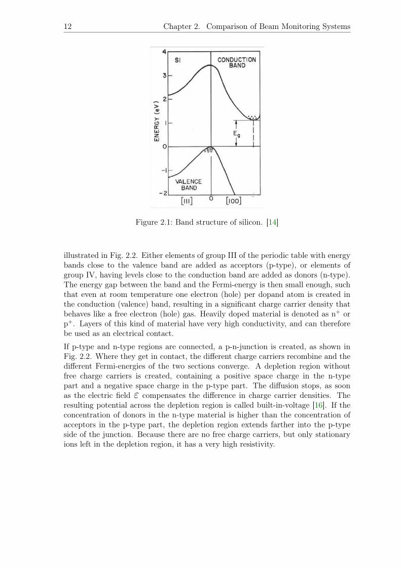
Silicon detectors are used for the detection of charged particles or photons in manydifferent applications. The basic principle is always the same, although the designof a specific detector can vary significantly. Silicon is a semiconductor with diamondcrystal structure, a lattice constant of 5.43Å, and a band gap of Eg = 1.12 eV, seeFig. 2.1. [15] As silicon is an indirect semiconductor, the production of an electron-hole pair requires a larger energy, on average 3.62 eV at room temperature [16]because additional phonon scattering is needed for the direct transition, as alsoillustrated in Fig. 2.1. Therefore, the incidence of this process is suppressed. Siliconis sensitive to a wide range of ionizing radiation, including visible light (E ≈ 2−4 eV)and X-rays, as well as ions or high-energy electrons.
At absolute zero, a semiconductor is an insulator, but at finite temperatures theconduction band is occupied by thermally excited electrons, leaving behind holes inthe valence band. The amount of electrons in the conduction band is given by theFermi-Dirac statistics. At room temperature only a fraction of 1 out of 1012 atomsis ionized. [17]
p-n-Junction
In principle, pure silicon could serve as a detector for ionizing radiation: Electronsfrom the valance band are excited to the conduction band and can be measured asa current. However, for technical applications the current is too low because theintrinsic charge carrier density is much too small. It can be increased by doping as
12 Chapter 2. Comparison of Beam Monitoring Systems
Figure 2.1: Band structure of silicon. [14]
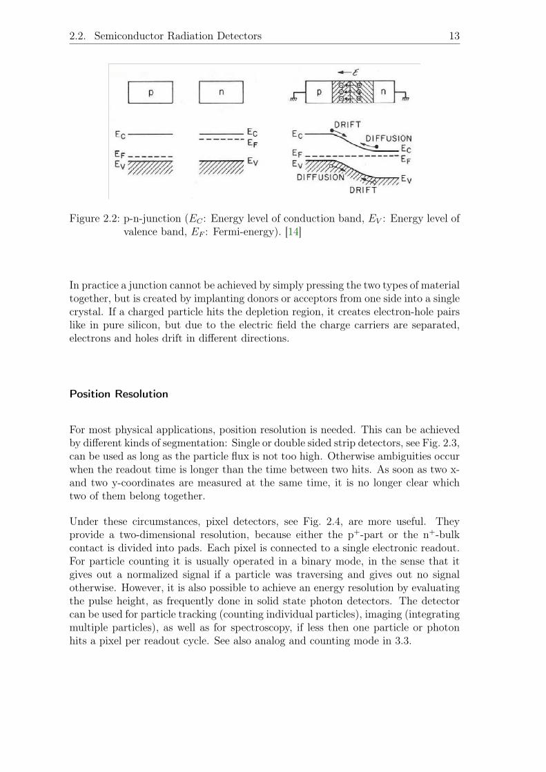
illustrated in Fig. 2.2. Either elements of group III of the periodic table with energybands close to the valence band are added as acceptors (p-type), or elements ofgroup IV, having levels close to the conduction band are added as donors (n-type).The energy gap between the band and the Fermi-energy is then small enough, suchthat even at room temperature one electron (hole) per dopand atom is created inthe conduction (valence) band, resulting in a significant charge carrier density thatbehaves like a free electron (hole) gas. Heavily doped material is denoted as n+ orp+. Layers of this kind of material have very high conductivity, and can thereforebe used as an electrical contact.
If p-type and n-type regions are connected, a p-n-junction is created, as shown inFig. 2.2. Where they get in contact, the different charge carriers recombine and thedifferent Fermi-energies of the two sections converge. A depletion region withoutfree charge carriers is created, containing a positive space charge in the n-typepart and a negative space charge in the p-type part. The diffusion stops, as soonas the electric field ε compensates the difference in charge carrier densities. Theresulting potential across the depletion region is called built-in-voltage [16]. If theconcentration of donors in the n-type material is higher than the concentration ofacceptors in the p-type part, the depletion region extends farther into the p-typeside of the junction. Because there are no free charge carriers, but only stationaryions left in the depletion region, it has a very high resistivity.
2.2. Semiconductor Radiation Detectors 13
Figure 2.2: p-n-junction (EC : Energy level of conduction band, EV : Energy level ofvalence band, EF : Fermi-energy). [14]
In practice a junction cannot be achieved by simply pressing the two types of materialtogether, but is created by implanting donors or acceptors from one side into a singlecrystal. If a charged particle hits the depletion region, it creates electron-hole pairslike in pure silicon, but due to the electric field the charge carriers are separated,electrons and holes drift in different directions.
Position Resolution
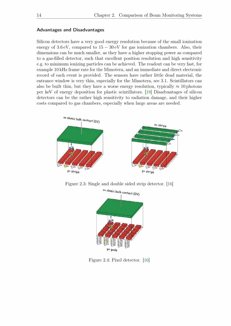
For most physical applications, position resolution is needed. This can be achievedby different kinds of segmentation: Single or double sided strip detectors, see Fig. 2.3,can be used as long as the particle flux is not too high. Otherwise ambiguities occurwhen the readout time is longer than the time between two hits. As soon as two x-and two y-coordinates are measured at the same time, it is no longer clear whichtwo of them belong together.
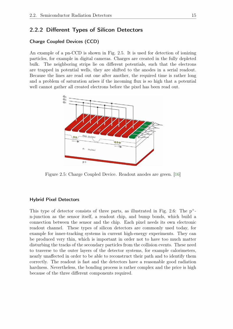
Under these circumstances, pixel detectors, see Fig. 2.4, are more useful. Theyprovide a two-dimensional resolution, because either the p+-part or the n+-bulkcontact is divided into pads. Each pixel is connected to a single electronic readout.For particle counting it is usually operated in a binary mode, in the sense that itgives out a normalized signal if a particle was traversing and gives out no signalotherwise. However, it is also possible to achieve an energy resolution by evaluatingthe pulse height, as frequently done in solid state photon detectors. The detectorcan be used for particle tracking (counting individual particles), imaging (integratingmultiple particles), as well as for spectroscopy, if less then one particle or photonhits a pixel per readout cycle. See also analog and counting mode in 3.3.
14 Chapter 2. Comparison of Beam Monitoring Systems
Advantages and Disadvantages
Silicon detectors have a very good energy resolution because of the small ionizationenergy of 3.6 eV, compared to 15 − 30 eV for gas ionization chambers. Also, theirdimensions can be much smaller, as they have a higher stopping power as comparedto a gas-filled detector, such that excellent position resolution and high sensitivitye.g. to minimum ionizing particles can be achieved. The readout can be very fast, forexample 10 kHz frame rate for the Mimotera, and an immediate and direct electronicrecord of each event is provided. The sensors have rather little dead material, theentrance window is very thin, especially for the Mimotera, see 3.1. Scintillators canalso be built thin, but they have a worse energy resolution, typically ≈ 10 photonsper keV of energy deposition for plastic scintillators. [18] Disadvantages of silicondetectors can be the rather high sensitivity to radiation damage, and their highercosts compared to gas chambers, especially when large areas are needed.
Figure 2.3: Single and double sided strip detector. [16]
Figure 2.4: Pixel detector. [16]
2.2. Semiconductor Radiation Detectors 15
2.2.2 Different Types of Silicon Detectors
Charge Coupled Devices (CCD)
An example of a pn-CCD is shown in Fig. 2.5. It is used for detection of ionizingparticles, for example in digital cameras. Charges are created in the fully depletedbulk. The neighboring strips lie on different potentials, such that the electronsare trapped in potential wells, they are shifted to the anodes in a serial readout.Because the lines are read out one after another, the required time is rather longand a problem of saturation arises if the incoming flux is so high that a potentialwell cannot gather all created electrons before the pixel has been read out.
Figure 2.5: Charge Coupled Device. Readout anodes are green. [16]
Hybrid Pixel Detectors
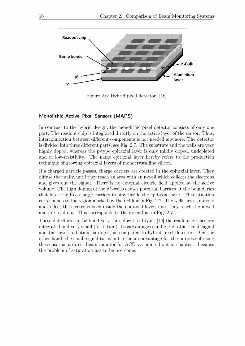
This type of detector consists of three parts, as illustrated in Fig. 2.6: The p+-n-junction as the sensor itself, a readout chip, and bump bonds, which build aconnection between the sensor and the chip. Each pixel needs its own electronicreadout channel. These types of silicon detectors are commonly used today, forexample for inner-tracking systems in current high-energy experiments. They canbe produced very thin, which is important in order not to have too much matterdisturbing the tracks of the secondary particles from the collision events. These needto traverse to the outer layers of the detector systems, for example calorimeters,nearly unaffected in order to be able to reconstruct their path and to identify themcorrectly. The readout is fast and the detectors have a reasonable good radiationhardness. Nevertheless, the bonding process is rather complex and the price is highbecause of the three different components required.
16 Chapter 2. Comparison of Beam Monitoring Systems
Figure 2.6: Hybrid pixel detector. [16]
Monolithic Active Pixel Sensors (MAPS)
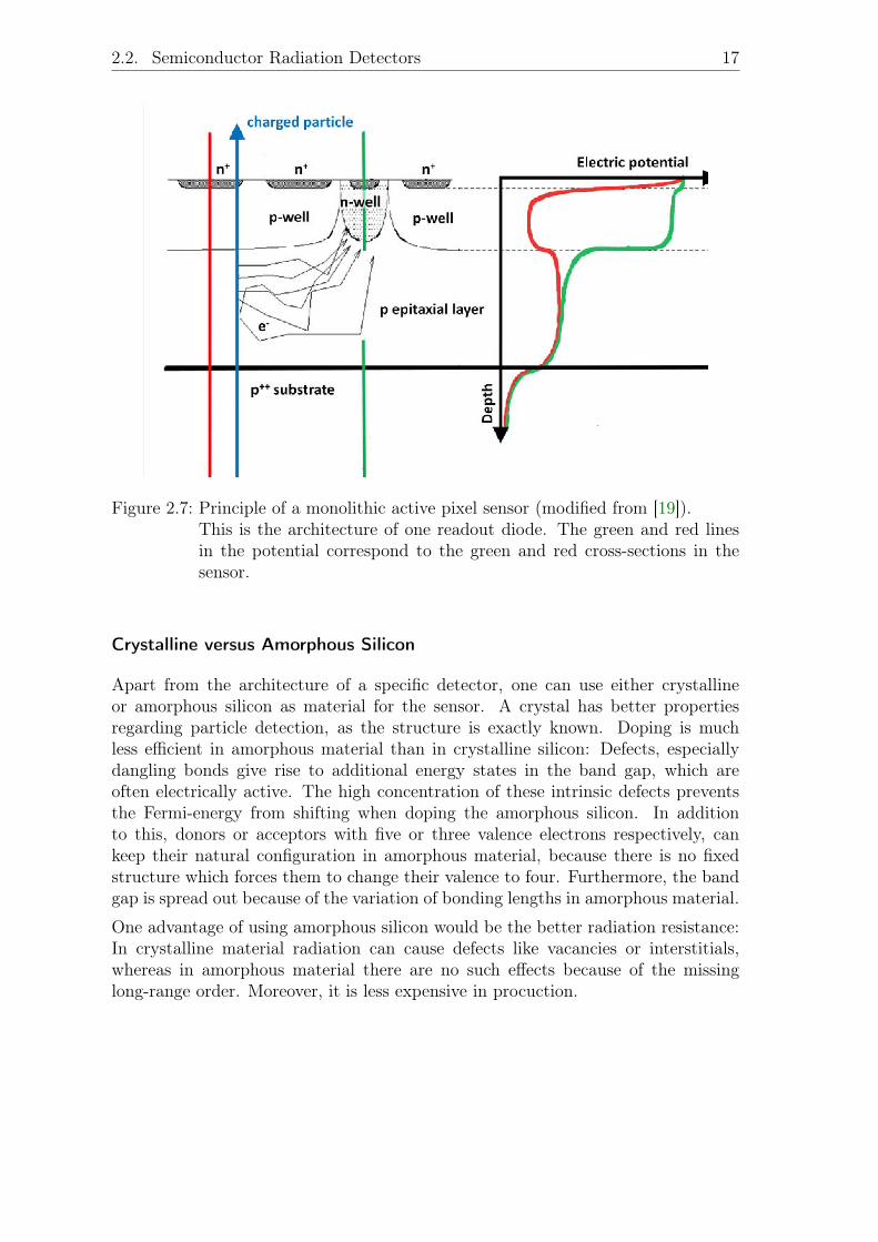
In contrast to the hybrid design, the monolithic pixel detector consists of only onepart. The readout chip is integrated directly on the active layer of the sensor. Thus,interconnection between different components is not needed anymore. The detectoris divided into three different parts, see Fig. 2.7. The substrate and the wells are veryhighly doped, whereas the p-type epitaxial layer is only mildly doped, undepletedand of low-resistivity. The name epitaxial layer hereby refers to the productiontechnique of growing epitaxial layers of monocrystalline silicon.
If a charged particle passes, charge carriers are created in the epitaxial layer. Theydiffuse thermally, until they reach an area with an n-well which collects the electronsand gives out the signal. There is no external electric field applied at the activevolume. The high doping of the p+-wells causes potential barriers at the boundariesthat force the free charge carriers to stay inside the epitaxial layer. This situationcorresponds to the region marked by the red line in Fig. 2.7. The wells act as mirrorsand reflect the electrons back inside the epitaxial layer, until they reach the n-welland are read out. This corresponds to the green line in Fig. 2.7.
These detectors can be build very thin, down to 14µm, [19] the readout pitches areintegrated and very small (5−50µm). Disadvantages can be the rather small signaland the lower radiation hardness, as compared to hybrid pixel detectors. On theother hand, the small signal turns out to be an advantage for the purpose of usingthe sensor as a direct beam monitor for ACE, as pointed out in chapter 1 becausethe problem of saturation has to be overcome.
2.2. Semiconductor Radiation Detectors 17
Figure 2.7: Principle of a monolithic active pixel sensor (modified from [19]).This is the architecture of one readout diode. The green and red linesin the potential correspond to the green and red cross-sections in thesensor.
Crystalline versus Amorphous Silicon
Apart from the architecture of a specific detector, one can use either crystallineor amorphous silicon as material for the sensor. A crystal has better propertiesregarding particle detection, as the structure is exactly known. Doping is muchless efficient in amorphous material than in crystalline silicon: Defects, especiallydangling bonds give rise to additional energy states in the band gap, which areoften electrically active. The high concentration of these intrinsic defects preventsthe Fermi-energy from shifting when doping the amorphous silicon. In additionto this, donors or acceptors with five or three valence electrons respectively, cankeep their natural configuration in amorphous material, because there is no fixedstructure which forces them to change their valence to four. Furthermore, the bandgap is spread out because of the variation of bonding lengths in amorphous material.
One advantage of using amorphous silicon would be the better radiation resistance:In crystalline material radiation can cause defects like vacancies or interstitials,whereas in amorphous material there are no such effects because of the missinglong-range order. Moreover, it is less expensive in procuction.

3 The Mimotera
3.1 Architecture of the Sensor
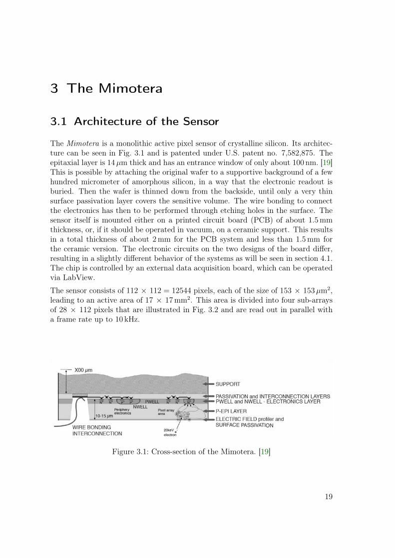
The Mimotera is a monolithic active pixel sensor of crystalline silicon. Its architec-ture can be seen in Fig. 3.1 and is patented under U.S. patent no. 7,582,875. Theepitaxial layer is 14µm thick and has an entrance window of only about 100 nm. [19]This is possible by attaching the original wafer to a supportive background of a fewhundred micrometer of amorphous silicon, in a way that the electronic readout isburied. Then the wafer is thinned down from the backside, until only a very thinsurface passivation layer covers the sensitive volume. The wire bonding to connectthe electronics has then to be performed through etching holes in the surface. Thesensor itself is mounted either on a printed circuit board (PCB) of about 1.5 mmthickness, or, if it should be operated in vacuum, on a ceramic support. This resultsin a total thickness of about 2 mm for the PCB system and less than 1.5 mm forthe ceramic version. The electronic circuits on the two designs of the board differ,resulting in a slightly different behavior of the systems as will be seen in section 4.1.The chip is controlled by an external data acquisition board, which can be operatedvia LabView.
The sensor consists of 112 × 112 = 12544 pixels, each of the size of 153 × 153µm2,leading to an active area of 17 × 17 mm2. This area is divided into four sub-arraysof 28 × 112 pixels that are illustrated in Fig. 3.2 and are read out in parallel witha frame rate up to 10 kHz.
Figure 3.1: Cross-section of the Mimotera. [19]
19
20 Chapter 3. The Mimotera
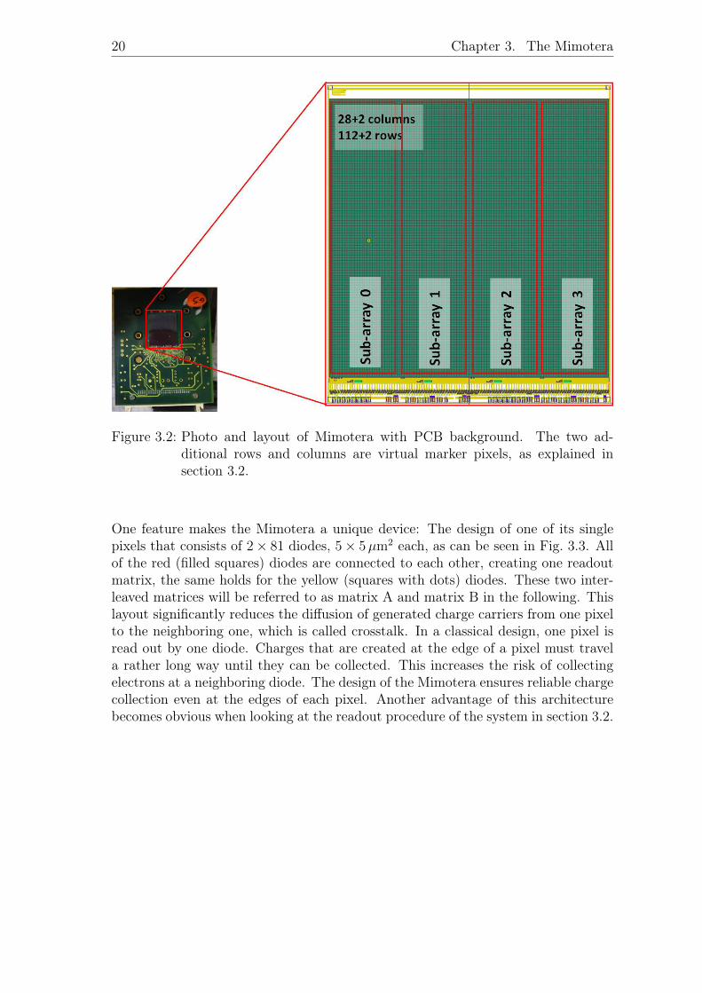
Figure 3.2: Photo and layout of Mimotera with PCB background. The two ad-ditional rows and columns are virtual marker pixels, as explained insection 3.2.
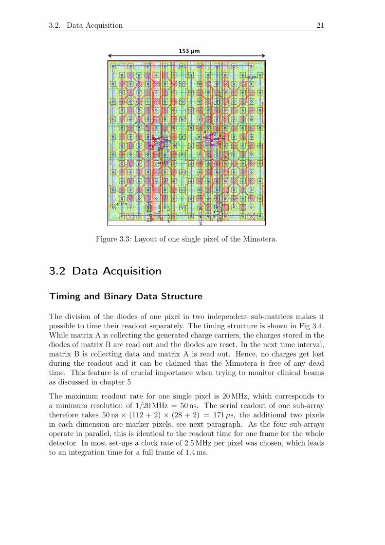
One feature makes the Mimotera a unique device: The design of one of its singlepixels that consists of 2× 81 diodes, 5× 5µm2 each, as can be seen in Fig. 3.3. Allof the red (filled squares) diodes are connected to each other, creating one readoutmatrix, the same holds for the yellow (squares with dots) diodes. These two inter-leaved matrices will be referred to as matrix A and matrix B in the following. Thislayout significantly reduces the diffusion of generated charge carriers from one pixelto the neighboring one, which is called crosstalk. In a classical design, one pixel isread out by one diode. Charges that are created at the edge of a pixel must travela rather long way until they can be collected. This increases the risk of collectingelectrons at a neighboring diode. The design of the Mimotera ensures reliable chargecollection even at the edges of each pixel. Another advantage of this architecturebecomes obvious when looking at the readout procedure of the system in section 3.2.
3.2. Data Acquisition 21
Figure 3.3: Layout of one single pixel of the Mimotera.
3.2 Data Acquisition
Timing and Binary Data Structure
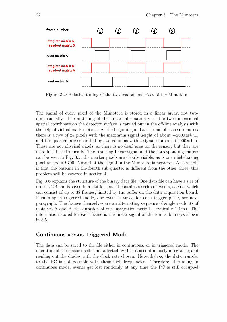
The division of the diodes of one pixel in two independent sub-matrices makes itpossible to time their readout separately. The timing structure is shown in Fig 3.4.While matrix A is collecting the generated charge carriers, the charges stored in thediodes of matrix B are read out and the diodes are reset. In the next time interval,matrix B is collecting data and matrix A is read out. Hence, no charges get lostduring the readout and it can be claimed that the Mimotera is free of any deadtime. This feature is of crucial importance when trying to monitor clinical beamsas discussed in chapter 5.
The maximum readout rate for one single pixel is 20 MHz, which corresponds toa minimum resolution of 1/20 MHz = 50 ns. The serial readout of one sub-arraytherefore takes 50 ns × (112 + 2) × (28 + 2) = 171µs, the additional two pixelsin each dimension are marker pixels, see next paragraph. As the four sub-arraysoperate in parallel, this is identical to the readout time for one frame for the wholedetector. In most set-ups a clock rate of 2.5 MHz per pixel was chosen, which leadsto an integration time for a full frame of 1.4 ms.
22 Chapter 3. The Mimotera
Figure 3.4: Relative timing of the two readout matrices of the Mimotera.
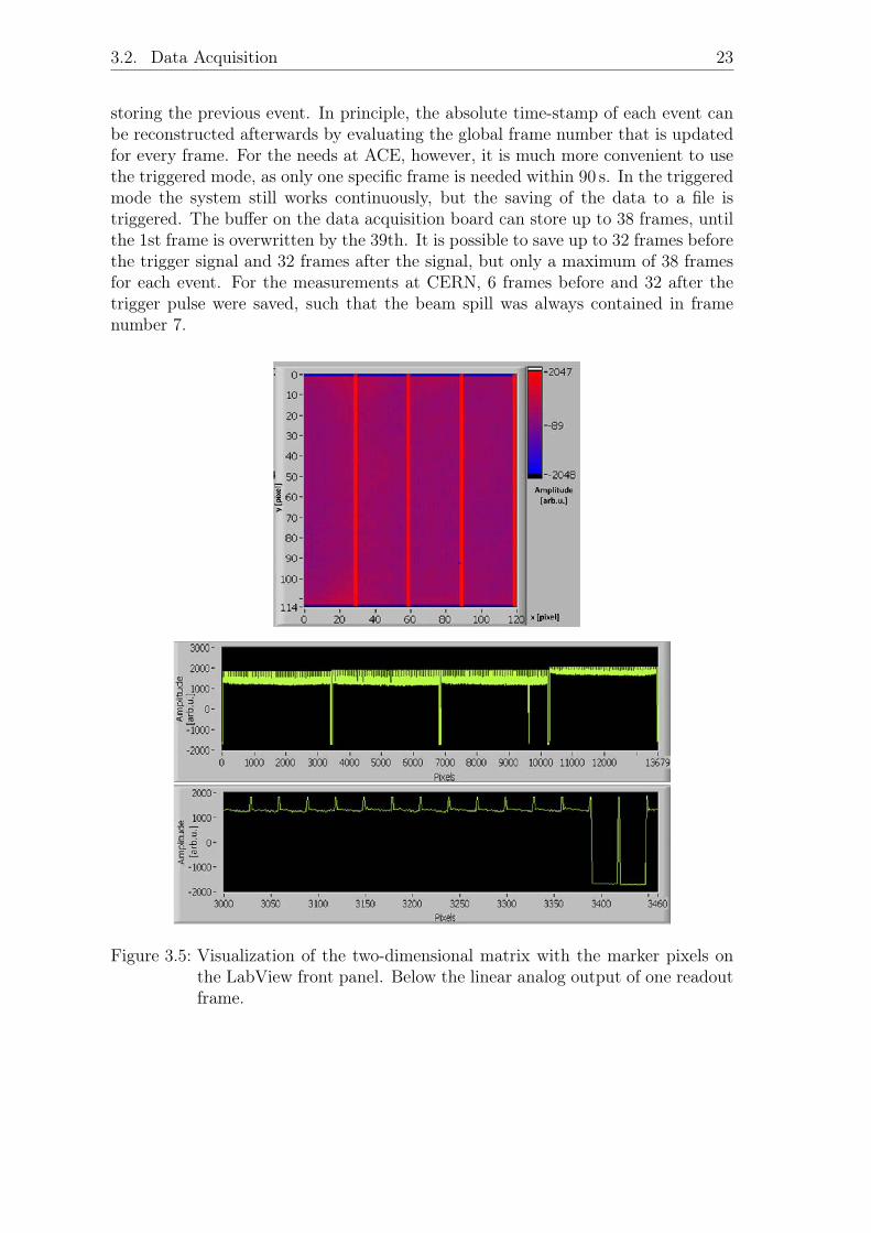
The signal of every pixel of the Mimotera is stored in a linear array, not two-dimensionally. The matching of the linear information with the two-dimensionalspatial coordinate on the detector surface is carried out in the off-line analysis withthe help of virtual marker pixels: At the beginning and at the end of each sub-matrixthere is a row of 28 pixels with the maximum signal height of about −2000 arb.u.,and the quarters are separated by two columns with a signal of about +2000 arb.u.These are not physical pixels, so there is no dead area on the sensor, but they areintroduced electronically. The resulting linear signal and the corresponding matrixcan be seen in Fig. 3.5, the marker pixels are clearly visible, as is one misbehavingpixel at about 9700. Note that the signal in the Mimotera is negative. Also visibleis that the baseline in the fourth sub-quarter is different from the other three, thisproblem will be covered in section 4.
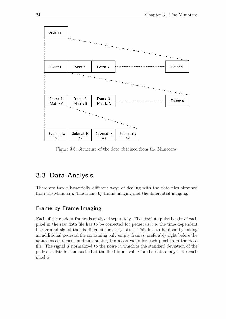
Fig. 3.6 explains the structure of the binary data file. One data file can have a size ofup to 2 GB and is saved in a .dat format. It contains a series of events, each of whichcan consist of up to 38 frames, limited by the buffer on the data acquisition board.If running in triggered mode, one event is saved for each trigger pulse, see nextparagraph. The frames themselves are an alternating sequence of single readouts ofmatrices A and B, the duration of one integration period is typically 1.4 ms. Theinformation stored for each frame is the linear signal of the four sub-arrays shownin 3.5.
Continuous versus Triggered Mode
The data can be saved to the file either in continuous, or in triggered mode. Theoperation of the sensor itself is not affected by this, it is continuously integrating andreading out the diodes with the clock rate chosen. Nevertheless, the data transferto the PC is not possible with these high frequencies. Therefore, if running incontinuous mode, events get lost randomly at any time the PC is still occupied
3.2. Data Acquisition 23
storing the previous event. In principle, the absolute time-stamp of each event canbe reconstructed afterwards by evaluating the global frame number that is updatedfor every frame. For the needs at ACE, however, it is much more convenient to usethe triggered mode, as only one specific frame is needed within 90 s. In the triggeredmode the system still works continuously, but the saving of the data to a file istriggered. The buffer on the data acquisition board can store up to 38 frames, untilthe 1st frame is overwritten by the 39th. It is possible to save up to 32 frames beforethe trigger signal and 32 frames after the signal, but only a maximum of 38 framesfor each event. For the measurements at CERN, 6 frames before and 32 after thetrigger pulse were saved, such that the beam spill was always contained in framenumber 7.
Figure 3.5: Visualization of the two-dimensional matrix with the marker pixels onthe LabView front panel. Below the linear analog output of one readoutframe.
24 Chapter 3. The Mimotera
Figure 3.6: Structure of the data obtained from the Mimotera.
3.3 Data Analysis
There are two substantially different ways of dealing with the data files obtainedfrom the Mimotera: The frame by frame imaging and the differential imaging.
Frame by Frame Imaging
Each of the readout frames is analyzed separately. The absolute pulse height of eachpixel in the raw data file has to be corrected for pedestals, i.e. the time dependentbackground signal that is different for every pixel. This has to be done by takingan additional pedestal file containing only empty frames, preferably right before theactual measurement and subtracting the mean value for each pixel from the datafile. The signal is normalized to the noise ν, which is the standard deviation of thepedestal distribution, such that the final input value for the data analysis for eachpixel is
3.3. Data Analysis 25
S(n) =pulse height(n)− pedestal
ν(3.1)
where n is the frame number. This calculation has to be performed for matricesA and B separately, as they are physically different and, therefore, have differentpedestals and noise levels. This mode is useful for continuous signals, for examplewhen imaging a laser spot.
Advantages: All values have the same polarity and details of the matrix structureare visible. For example the faulty pixel that is visible in Fig. 3.5 would disappearin an analysis with the differential mode.
Disadvantage: As mentioned above, it is necessary to keep exact track of thepedestals. This has to be done by taking additional data files, and even then thereis a systematic error if the pedestal shifts in between the background measurementand the taking of the actual data. The pedestals can vary strongly with time, whichis why a new method has been developed for the measurements at HIT, providingthe possibility of tracking them more closely in time to the actual data. This willbe described in chapter 5.
Differential Imaging
In this mode, not the absolute signal, but the difference between two subsequentframes is considered. Taking into account the timing structure in Fig. 3.4, thedifference is build for matrices A and B separately, such that for matrix A one getsframes 4-2, 6-4, 8-6, etc. and for matrix B frames 3-1, 5-3, 7-5, etc. The resultingsignal for each pixel is
∆(n) = pulse height(n)− pulse height(n-2) (3.2)
again, to be carried out separately for both matrices A and B.
Advantage: One does not need to consider the pedestals, as they can be expectedto be the same for two subsequent frames. The difference is thus zero and theydo not contribute to the signal. This method is very useful for the experimentalconditions at ACE, where the beam is contained in only one readout frame, andthus the difference of two frames results in the absolute signal.
Disadvantages: The resulting signal can be either positive or negative, dependingon the chronological order of the frames before subtraction. Details of the matrixstructure, like dead pixels, get lost as they are the same in every frame.
26 Chapter 3. The Mimotera
Analog versus Counting
Apart from the two different imaging modalities described above, there is anotherdistinction one can make in the analysis of the data. One possibility is to takeinto consideration the absolute, analog pulse height in each pixel, the other oneis to do particle counting. The Mimotera is able to do both. In the countingmode, a pixel can only be regarded as hit or not hit, the height of the signal iswithout relevance. This provides a direct measurement of the particle flux, withoutcalibration. A threshold has to be defined beforehand, above which a pixel countsas being hit, below as being not hit. For this method it is important to reduce thecrosstalk between neighboring pixels, in order not to count a particle twice. This ispossible due to the multiple readout diodes in each pixel described in 3.1. The mostimportant and severe limitation, however, is that it is not applicable in a pile-upsituation, namely if the flux is so high that the mean number of particles per pixelper frame exceeds one. In this case, two particles in the same pixel in the sameframe are only counted as one. Therefore this mode is only useful for low intensitybeams.
The analog method on the other hand can still be used even if the experimentalconditions lead to pile-up, as the absolute signal height for a monoenergetic beamdepends only on the number of particles hitting the pixel. This is valid as longas the dynamic range of the detector is not completely exhausted and saturationis reached. This is a challenge at ACE, as will be see in chapter 4. On the otherhand, the analog method requires a calibration for a measurement of the absoluteintensity, as otherwise it is not known how to interpret the pulse height of a signal.This calibration might even be time dependent.
At ACE there is definitely a situation of pile-up, as the intensity is 3 × 10⁷ particlesin one frame and the Mimotera has only 1.25 × 104 pixels. Therefore, the analogmode has to be used. Furthermore, it is convenient not to subtract the pedestals,especially because the spill of antiprotons is contained in only one readout frameand subtracting the pedestal is equal to simply subtracting the previous frame. Thisis the reason for choosing the differential imaging.
The analysis of the data is carried out with ROOT, a data analysis framework fromCERN, [20] using different macros written in C.

3.4. Why the Mimotera is the System of Choice 27
3.4 Why the Mimotera is the System of Choice
Thickness
The total thickness of the PCB system is about 2 mm. For the 126 MeV antiprotonsat ACE with a range of approximately 10 cm in water, this does not disturb theoperation significantly. The system is installed close to the water tank, so that theeffect caused by multiple scattering in the air between sensor and the cell sample isnegligible.
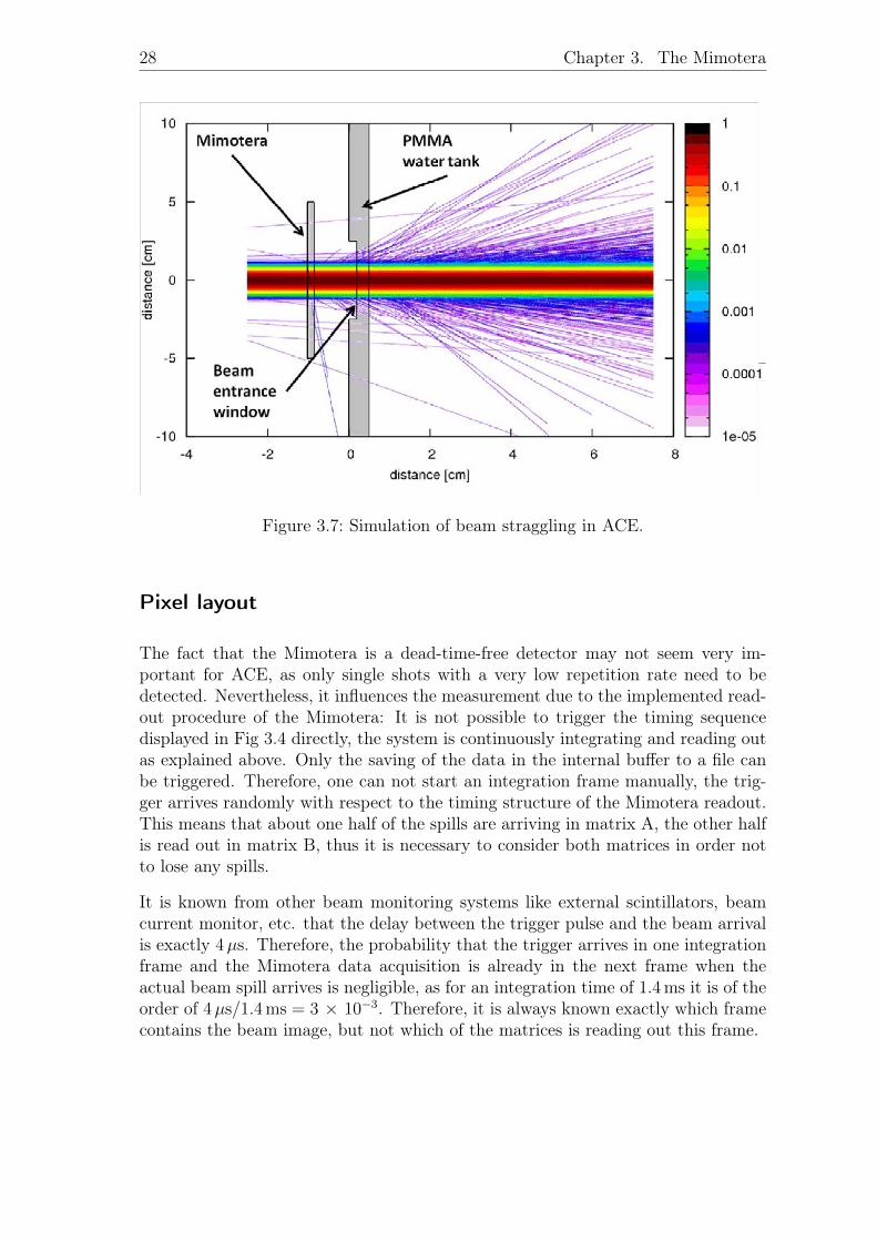
A Monte-Carlo-simulation has been performed with FLUKA, in order to comparethe beam straggling caused by the Mimotera, the air and the water tank. The resultscan be seen in Fig. 3.7. Distance zero along the beam direction indicates the edge ofthe PMMA water tank, which has an entrance window of 3 mm thickness. In frontof the tank, the Mimotera is mounted, both are surrounded by air. The additionalstraggling of the beam caused by the Mimotera is extremely small. The number ofparticles scattered by the system is of the order of only 0.01 % of the total numberof particles in the beam. Moreover, for modifying the energy of the beam in severalsteps to produce a spread-out Bragg-peak, degraders of 1 mm of PMMA are insertedin the beam line in front of the Mimotera. This increases the beam straggling byfar more, making it already necessary to account for it in the Monte Carlo dosecalculations. Thus, for the energy range interesting for ACE, the Mimotera is thinenough not to disturb the operation significantly.
Size
The active area of the Mimotera is only 17 × 17 mm. Thus it is not possible tomonitor beams with large diameters, for example de-focused clinical proton beamsas used at HIT, see section 5.1. Nevertheless, as the antiproton beam at ACE hasa FWHM of only about 7 mm, the Mimotera is large enough to monitor the wholebeam spot.
Position and Time Resolution
The spatial resolution of the sensor is 153µm. This is fully sufficient for the ACErequirements, because for a profile of 7 mm FWHM, about 7 mm/153µm = 45 datapoints are obtained in the central region. Therefore, the pixel size of the Mimoterais small enough to provide a good profile measurement of the beam. The high framerate of up to 10 kHz is not of major importance for the ACE set-up, but it will beimportant when monitoring continuous beams of protons and carbon ions at HIT,see chapter 5.
28 Chapter 3. The Mimotera
Figure 3.7: Simulation of beam straggling in ACE.
Pixel layout
The fact that the Mimotera is a dead-time-free detector may not seem very im-portant for ACE, as only single shots with a very low repetition rate need to bedetected. Nevertheless, it influences the measurement due to the implemented read-out procedure of the Mimotera: It is not possible to trigger the timing sequencedisplayed in Fig 3.4 directly, the system is continuously integrating and reading outas explained above. Only the saving of the data in the internal buffer to a file canbe triggered. Therefore, one can not start an integration frame manually, the trig-ger arrives randomly with respect to the timing structure of the Mimotera readout.This means that about one half of the spills are arriving in matrix A, the other halfis read out in matrix B, thus it is necessary to consider both matrices in order notto lose any spills.
It is known from other beam monitoring systems like external scintillators, beamcurrent monitor, etc. that the delay between the trigger pulse and the beam arrivalis exactly 4µs. Therefore, the probability that the trigger arrives in one integrationframe and the Mimotera data acquisition is already in the next frame when theactual beam spill arrives is negligible, as for an integration time of 1.4 ms it is of theorder of 4µs/1.4 ms = 3 × 10⁻³. Therefore, it is always known exactly which framecontains the beam image, but not which of the matrices is reading out this frame.
3.4. Why the Mimotera is the System of Choice 29
Dynamic range
The electric potential in each pixel of the Mimotera is U = 2 V, the capacitance canbe chosen to be C = 0.5 pF (called “attenuation off”) or 5 pF (called “attenuationon”), depending on which signal height is expected for a certain experimental set-up.As the particle flux at ACE is high in a short time interval, the larger capacitanceis chosen. This means that every pixel can store a charge of up to Q = CU =5 pF×2 V = 10−11 C, which corresponds to 10−11 C/(1.6×10−19 C) = 6×10⁷ electronsper pixel before reaching saturation. For the lower limit of charge carriers that canstill be detected as a signal, one has to consider the equivalent noise charge of thesensor. [21] For the Mimotera this is about about 1000 electron-hole pairs per pixel.A signal to noise ratio of the order of 5 is desirable, therefore about 5×10³ electronsper pixel per frame are needed to obtain a stable and reliable signal.
The energy loss through ionization and excitation of a 126 MeV proton in the 14µmepi-layer in the Mimotera is 16 keV, see also section 5.3. [25] For an antiproton theenergy loss can be considered to be equal, as for this energy the particles are farfrom being stopped in the volume, essentially no nuclear interactions take place andno annihilation events occur. The mean energy to create an electron-hole pair insilicon is 3.62 eV at room temperature, as stated in 2.2.1. This means that eachantiproton on average sets free 16 keV/3.62 eV = 4.4×10³ electrons when traversingthe epi-layer of the Mimotera, which is safely above the mean noise level, such thatsingle antiprotons could be detected. As a consequence, the upper limit of flux theMimotera can handle is about 6× 10⁷/(4.4× 103) = 1.4× 10⁴ antiprotons per pixel.
The number of antiprotons hitting one single pixel is highest in the center of theGaussian and is calculated as follows: The probability that a particle hits the de-tector at −x0 ≤ x ≤ x0, is
Px =
∫ +x0
x=−xo
1√2πσ2
e−x2/2σ2
dx (3.3)
with x0 = 153µm/2 = 76.5µm and σ = FWHM/2√
2 ln 2 = 7 mm/2√
2 ln 2 =2.97 mm. An expansion leads to
e−x2/2σ2
=∞∑i=0
(−x2/2σ2)i
i!= (1− x2
2σ2− ...) = 1 for x� σ (3.4)
Inserting this in the integral above yields
Px =
∫ x0
x=−xo
1√2πσ2
dx =2x0√2πσ2
(3.5)
30 Chapter 3. The Mimotera
As the distribution is symmetric, the probability of hitting the central pixel is
P = Px · Py =(2x0)
2
2πσ2=
(153µm)2
2π(2.97 mm)2= 4.2× 10⁻⁴ (3.6)
which leads to a total number of particles in the central pixel of
N = P ·N0 = 4.2× 10−4 · 3× 107 = 1.3× 10⁴ (3.7)
for a total beam intensity of 3× 10⁷ particles in one spill.
It has been calculated above that the Mimotera is able to cope with 1.4 × 10⁴
antiprotons per pixel with the attenuation turned on. Therefore, it can be expectedthat the sensor will be able to operate without saturation at ACE. The signal heightseems to lie just barely below the upper limit of the dynamic range, but one hasalso to consider that the estimation above holds only for an ideal sensor that collects100% of the charges generated in the active volume. This is of course not the casefor any such device, several different effects reduce the charge collection efficiency.Three examples for such effects are:
A build-up effect similar to the situation with photons explained in section 1.1 hasbeen observed also for carbon ions. It is of the order of some percent in a range ofabout 1 mm in PMMA. [22] The behavior of other ions like protons and antiprotonscan be considered to be very similar. As the Mimotera has an entrance window ofonly about 100 nm and the epitaxial layer is as thin as 14µm, the signal does notreach its full height within the active volume. This reduces the number of generatedcharge carriers by a few percent.
A second effect that could reduce the signal height, is recombination of electron-hole pairs that annihilate before they are read out. Usually this effect can be ne-glected, [24] because the space charge region separates electrons and holes veryquickly. Nevertheless, the Mimotera is a MAPS, in which no external voltage is ap-plied to deplete the sensor, the charges are collected via thermal diffusion. Therefore,the lifetime of a signal charge could be a significant parameter. Measurements withultra-thin silicon detectors in a 5 MeV antiproton beam have shown a significantreduction of the signal for lover bias voltages. [23]
Moreover, measurements at ACE have demonstrated that 15 readout cycles are notenough to collect all charge carriers generated in a single frame due to incompletereadout, see section 6.1. This reduces the height of the signal in the actual framewith the beam further, because a non-negligible fraction of the charges are collectedonly in the following frames.
In summary, the design of the Mimotera thus seems to be suitable for serving as anearly-non-disturbing, direct beam monitor for the Antiproton Cell Experiment.
4 Antiproton Beam at ACE
4.1 The Challenge of Saturation
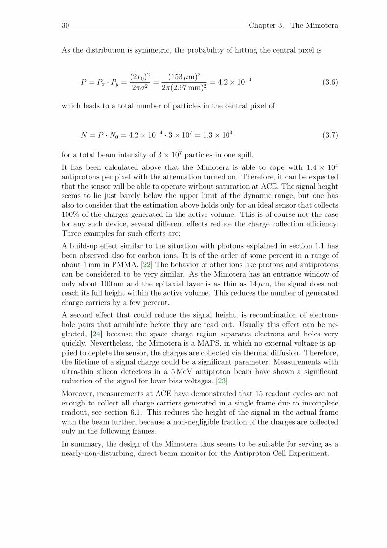
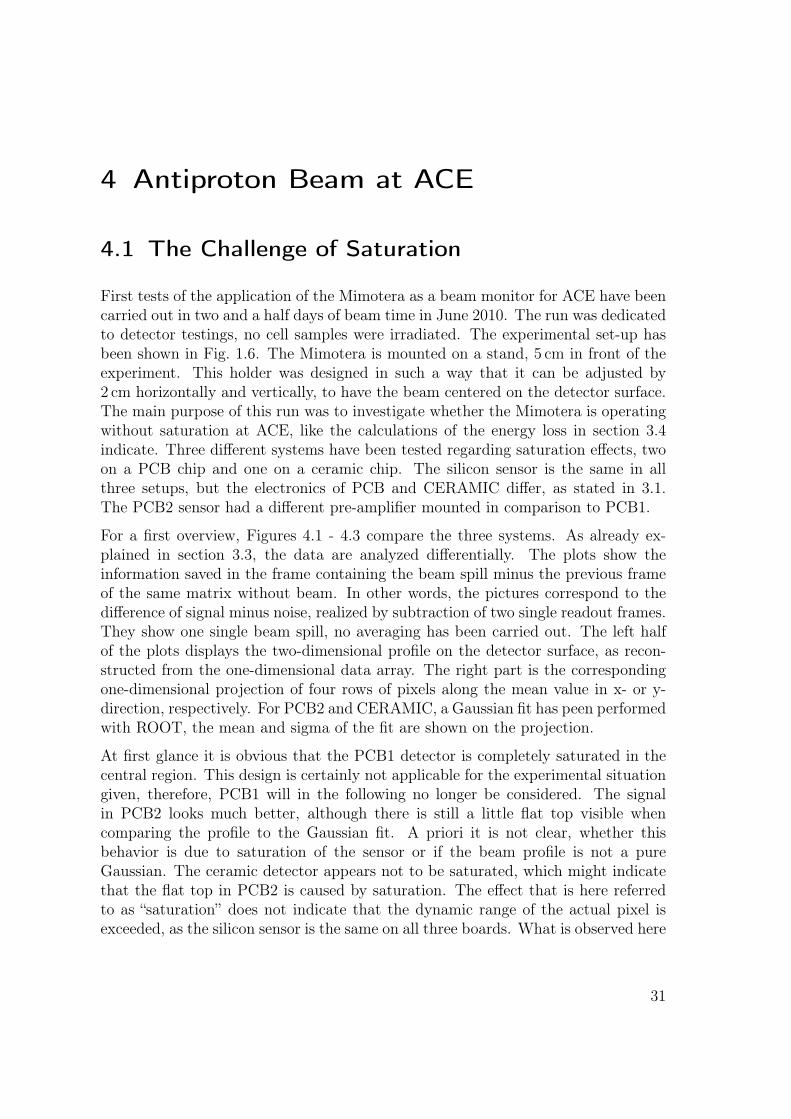
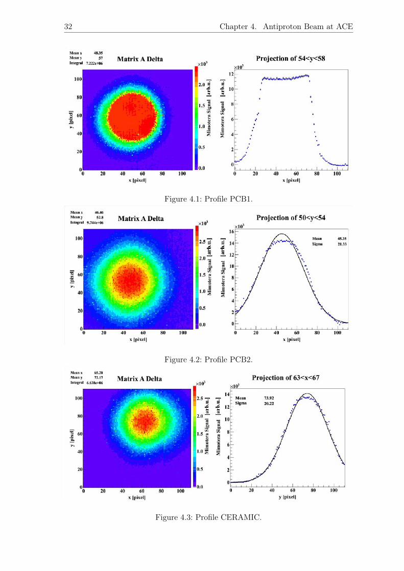
First tests of the application of the Mimotera as a beam monitor for ACE have beencarried out in two and a half days of beam time in June 2010. The run was dedicatedto detector testings, no cell samples were irradiated. The experimental set-up hasbeen shown in Fig. 1.6. The Mimotera is mounted on a stand, 5 cm in front of theexperiment. This holder was designed in such a way that it can be adjusted by2 cm horizontally and vertically, to have the beam centered on the detector surface.The main purpose of this run was to investigate whether the Mimotera is operatingwithout saturation at ACE, like the calculations of the energy loss in section 3.4indicate. Three different systems have been tested regarding saturation effects, twoon a PCB chip and one on a ceramic chip. The silicon sensor is the same in allthree setups, but the electronics of PCB and CERAMIC differ, as stated in 3.1.The PCB2 sensor had a different pre-amplifier mounted in comparison to PCB1.
For a first overview, Figures 4.1 - 4.3 compare the three systems. As already ex-plained in section 3.3, the data are analyzed differentially. The plots show theinformation saved in the frame containing the beam spill minus the previous frameof the same matrix without beam. In other words, the pictures correspond to thedifference of signal minus noise, realized by subtraction of two single readout frames.They show one single beam spill, no averaging has been carried out. The left halfof the plots displays the two-dimensional profile on the detector surface, as recon-structed from the one-dimensional data array. The right part is the correspondingone-dimensional projection of four rows of pixels along the mean value in x- or y-direction, respectively. For PCB2 and CERAMIC, a Gaussian fit has peen performedwith ROOT, the mean and sigma of the fit are shown on the projection.
At first glance it is obvious that the PCB1 detector is completely saturated in thecentral region. This design is certainly not applicable for the experimental situationgiven, therefore, PCB1 will in the following no longer be considered. The signalin PCB2 looks much better, although there is still a little flat top visible whencomparing the profile to the Gaussian fit. A priori it is not clear, whether thisbehavior is due to saturation of the sensor or if the beam profile is not a pureGaussian. The ceramic detector appears not to be saturated, which might indicatethat the flat top in PCB2 is caused by saturation. The effect that is here referredto as “saturation” does not indicate that the dynamic range of the actual pixel isexceeded, as the silicon sensor is the same on all three boards. What is observed here
31
32 Chapter 4. Antiproton Beam at ACE
Figure 4.1: Profile PCB1.
Figure 4.2: Profile PCB2.
Figure 4.3: Profile CERAMIC.
4.1. The Challenge of Saturation 33
is merely a saturation of the on-board electronics that can be reduced by exchangingthe amplifier, as can be seen for PCB2.
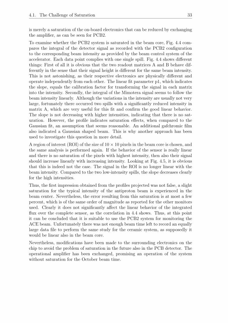
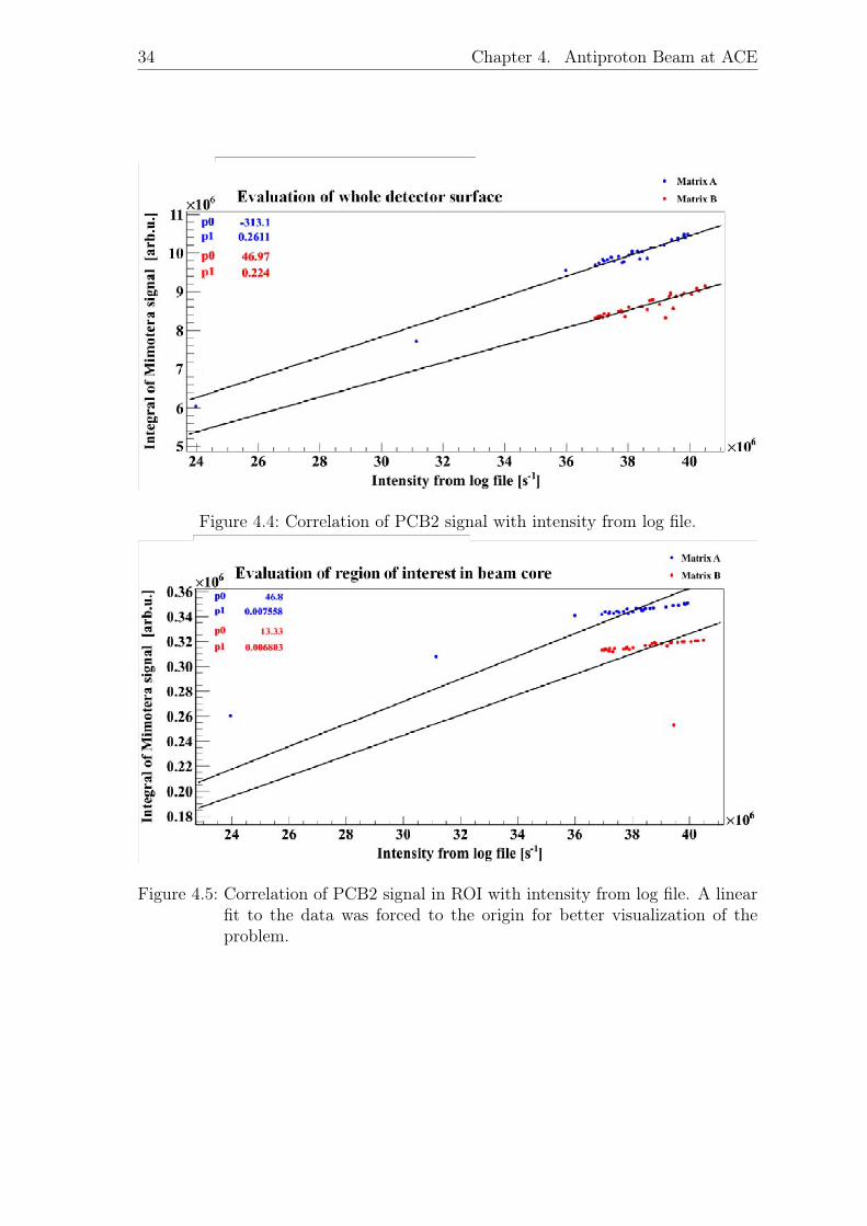
To examine whether the PCB2 system is saturated in the beam core, Fig. 4.4 com-pares the integral of the detector signal as recorded with the PCB2 configurationto the corresponding beam intensity as provided by the beam control system of theaccelerator. Each data point complies with one single spill. Fig. 4.4 shows differentthings: First of all it is obvious that the two readout matrices A and B behave dif-ferently in the sense that their signal height is different for the same beam intensity.This is not astonishing, as their respective electronics are physically different andoperate independently from each other. The linear fit parameter p1, which indicatesthe slope, equals the calibration factor for transforming the signal in each matrixinto the intensity. Secondly, the integral of the Mimotera signal seems to follow thebeam intensity linearly. Although the variations in the intensity are usually not verylarge, fortunately there occurred two spills with a significantly reduced intensity inmatrix A, which are very useful for this fit and confirm the good linear behavior.The slope is not decreasing with higher intensities, indicating that there is no sat-uration. However, the profile indicates saturation effects, when compared to theGaussian fit, an assumption that seems reasonable. An additional gafchromic filmalso indicated a Gaussian shaped beam. This is why another approach has beenused to investigate this question in more detail.
A region of interest (ROI) of the size of 10× 10 pixels in the beam core is chosen, andthe same analysis is performed again. If the behavior of the sensor is really linearand there is no saturation of the pixels with highest intensity, then also their signalshould increase linearly with increasing intensity. Looking at Fig. 4.5, it is obviousthat this is indeed not the case. The signal in the ROI is no longer linear with thebeam intensity. Compared to the two low-intensity spills, the slope decreases clearlyfor the high intensities.
Thus, the first impression obtained from the profiles projected was not false, a slightsaturation for the typical intensity of the antiproton beam is experienced in thebeam center. Nevertheless, the error resulting from this saturation is at most a fewpercent, which is of the same order of magnitude as reported for the other monitorsused. Clearly it does not significantly affect the linear behavior of the integratedflux over the complete sensor, as the correlation in 4.4 shows. Thus, at this pointit can be concluded that it is suitable to use the PCB2 system for monitoring theACE beam. Unfortunately there was not enough beam time left to record an equallylarge data file to perform the same study for the ceramic system, as supposedly itwould be linear also in the beam core.
Nevertheless, modifications have been made to the surrounding electronics on thechip to avoid the problem of saturation in the future also in the PCB detector. Theoperational amplifier has been exchanged, promising an operation of the systemwithout saturation for the October beam time.
34 Chapter 4. Antiproton Beam at ACE
Figure 4.4: Correlation of PCB2 signal with intensity from log file.
Figure 4.5: Correlation of PCB2 signal in ROI with intensity from log file. A linearfit to the data was forced to the origin for better visualization of theproblem.

4.1. The Challenge of Saturation 35
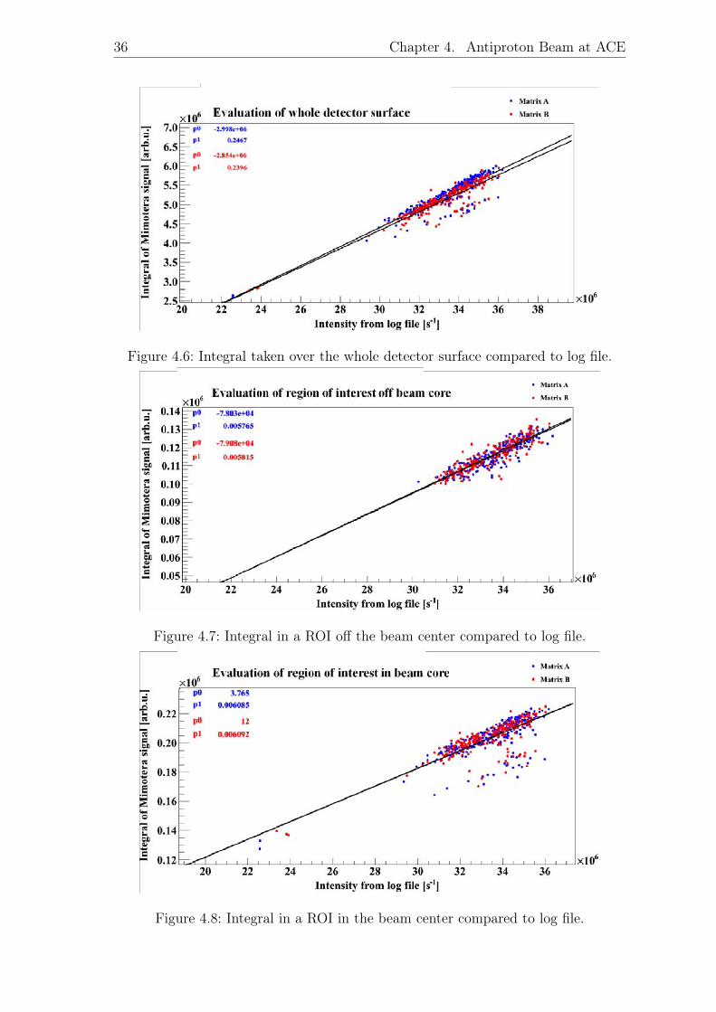
The same analysis as explained above has then been performed for a larger data file,taken with the PCB2 detector in October 2010. Fig. 4.6 corresponds to Fig. 4.4,Fig. 4.8 correlates with Fig. 4.5. The behavior of the sensor is now linear withincreasing intensities, even in the core of the beam. Also, the relation of signalheights in matrix A and B changed with respect to the set-up in June: The twomatrices are behaving nearly identical now, there is no longer a shift between theirintegrals.
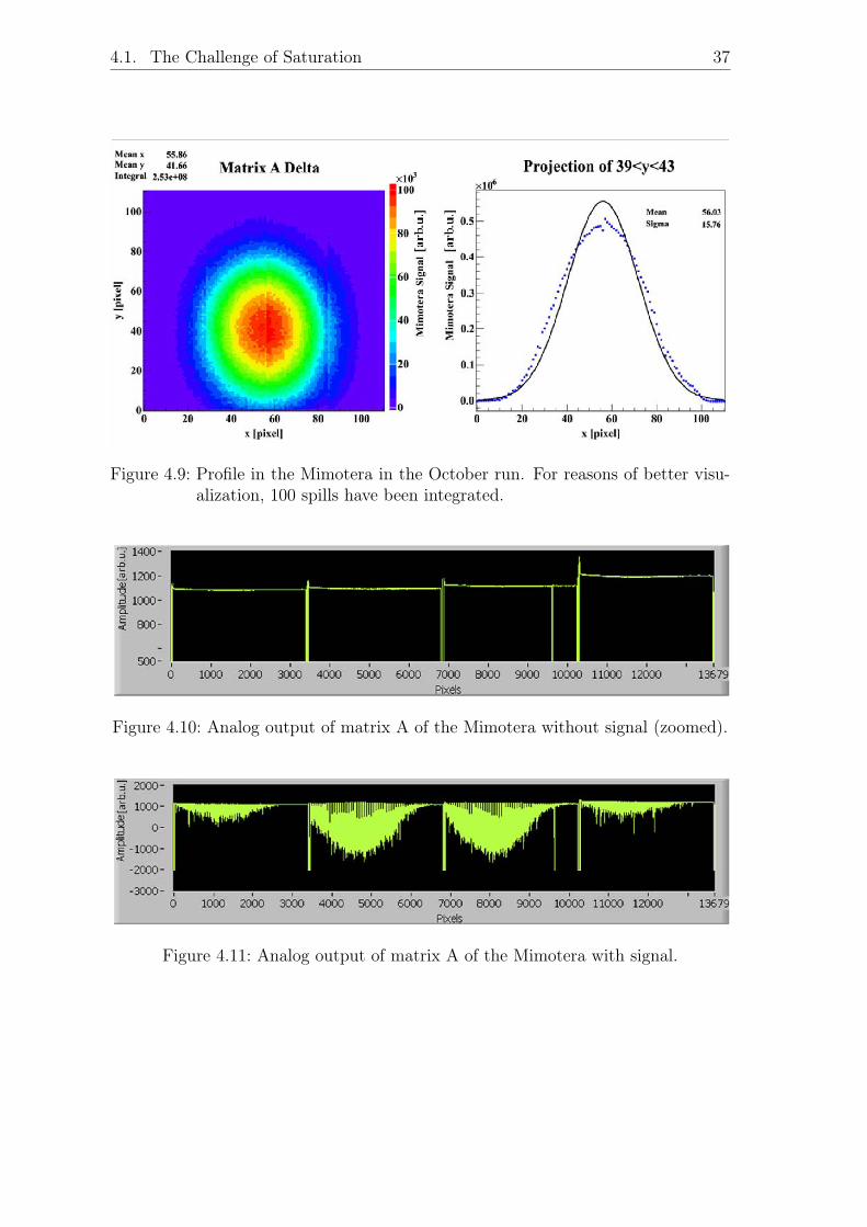
Unfortunately, a different effect occurs for the October data: The linear fit in Fig. 4.6and Fig. 4.8 does no longer cross zero. This is not the case when taking into account aROI in the core of the beam, see Fig. 4.8. As the analysis is carried out differentially,this can not be a constant offset in the pixels because this would cancel out in thesubtraction. It might be related to an effect that becomes visible when lookingat the two-dimensional beam-profiles from the October run, one of which is shownin Fig. 4.9. There is a shift in the signal of one sub-quarter with respect to theneighboring one. This problem is caused by different baselines in each sub-quarter,as can be seen in the corresponding analog output of the matrix without beam inFig. 4.10. The difference between the third and the fourth sub-matrix is largest,causing a discontinuity along the x-axis in the two-dimensional profile of each beamspill, see Fig. 4.9. This effect might have been already present in one of the sub-quarters in the set-up used in June, as indicated by Fig. 3.5. Nevertheless, it did notaffect the profiles obtained in this run, because the beam was slightly shifted awayfrom the center of the Mimotera, such that this particular sub-quarter was nearlynot irradiated at all.
All efforts during the October beam time to eliminate these shifts failed, neitherexchanging the cables, the DAQ board, or even the sensor itself, nor tuning the op-eration voltage on the DAQ board improved the situation substantially. Still, thisconstant offset should not disturb the differential analysis, and it is not yet under-stood why this effect is observed even after subtraction. This has to be investigatedfurther for future beam times.
Nevertheless, the problem of saturation has been solved for the system used in theOctober run, as the correlation with the CERN log file is linear and as the amplitudesin Fig. 4.11 are below the saturation limit. The signal height of −2000 arb.u. of themarker pixels indicates the maximum possible signal height in the sensor. Rememberthat the signal in the Mimotera is negative. The dynamic range is not fully exploitedin this case. The estimation in section 3.4 indicated that the antiproton beam needs1.3/1.4 = 93% of the dynamic range. Looking at Fig. 4.11, the signal seems tobe smaller than this, leading to the conclusion that the signal is indeed somewhatreduced by the effects described in section 3.4.
36 Chapter 4. Antiproton Beam at ACE
Figure 4.6: Integral taken over the whole detector surface compared to log file.
Figure 4.7: Integral in a ROI off the beam center compared to log file.
Figure 4.8: Integral in a ROI in the beam center compared to log file.
4.1. The Challenge of Saturation 37
Figure 4.9: Profile in the Mimotera in the October run. For reasons of better visu-alization, 100 spills have been integrated.
Figure 4.10: Analog output of matrix A of the Mimotera without signal (zoomed).
Figure 4.11: Analog output of matrix A of the Mimotera with signal.
38 Chapter 4. Antiproton Beam at ACE
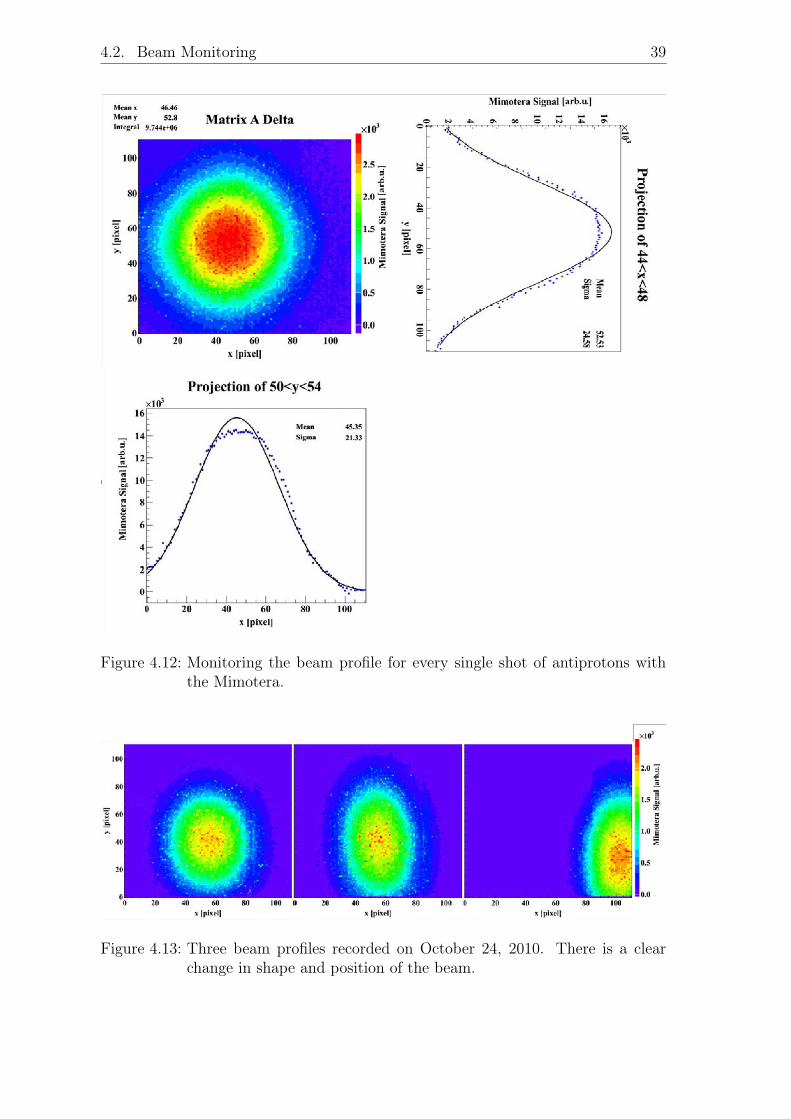
4.2 Beam Monitoring
As stated in section 1.3, the future beam monitor for ACE shall provide a real-time,digital image of the beam profile and it shall track the fluctuations in beam intensityand position. The data analysis is performed in a way that all three quantities canbe obtained quickly for each data file. For the beam profile, the two-dimensionalplots along with projections in x- and y- directions are saved for every single shot,and one example is given in Fig. 4.12. Note that the data is taken from the PCB2system in June, and therefore the small saturation effect is still visible.
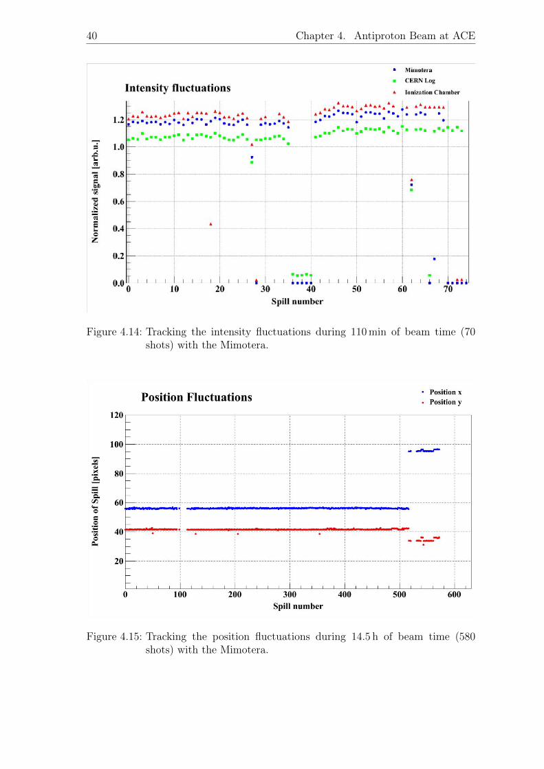
For a real-time, online image of the beam, a two-dimensional beam profile andprojections in x- and y-directions have also been implemented on the LabView frontpanel. This offers the possibility to recognize and correct a sudden change in profileor position of the beam within only one shot, as can be seen in Fig 4.13, taken onOctober 24, 2010. The cell sample can be removed from the water tank immediately,until the beam has been re-adjusted, and thus incorrect irradiation of the cell sampleby more than one spill can be avoided. Using only a gafchromic film, this changewould have been realized only after a long time, if at all, and the cell sample wouldhave been totally lost for the data set.
The progression of the beam intensity is displayed by plotting the integral of theMimotera signal for a consecutive spill number, see Fig. 4.14. In order to investi-gate the reliability of the accelerator log and the ionization chamber signals, theircorresponding measurements are plotted as well. All are normalized to their inte-gral over the spill number to fit on the same scale. In general, the course of theMimotera signal follows the intensity of the log file very well. It seems to be at leastas accurate in tracking relative changes of the beam intensity from shot to shot asthe calibrated ionization chamber, and thus can be used to monitor the intensityfluctuations during an irradiation. This will allow to correct for occasional readouterrors observed to occur for the ionization chamber, caused by trigger problems ofthe main control software of the experiment, as for example for spills 31, 32, 59 and60. For spills 36–40, the signals of the Mimotera and of the ionization chamber lieon top of each other.
The two-dimensional beam position is defined by the mean values of the beam profilein x- and y-directions respectively, and is tracked in a similar plot. It is usually verystable, with maximum fluctuations of less than two pixels (300µm) along the x-,and even less, about one pixel along the y-direction. Nevertheless, in October asituation occured that demonstrated the major improvement that the Mimoteraoffers for ACE. Fig. 4.15 shows the position tracking over a period of 14 hours ofbeam time. There was a sudden, large change in the beam position at spill number517 that would have been disastrous for the cell irradiation, if unnoticed.
4.2. Beam Monitoring 39
Figure 4.12: Monitoring the beam profile for every single shot of antiprotons withthe Mimotera.
Figure 4.13: Three beam profiles recorded on October 24, 2010. There is a clearchange in shape and position of the beam.
40 Chapter 4. Antiproton Beam at ACE
Figure 4.14: Tracking the intensity fluctuations during 110 min of beam time (70shots) with the Mimotera.
Figure 4.15: Tracking the position fluctuations during 14.5 h of beam time (580shots) with the Mimotera.

4.3. The Mimotera as an Alignment Tool 41
4.3 The Mimotera as an Alignment Tool
The Mimotera proved to be an excellent choice not only for the tracking of the beamintensity and position, but also for substantially improving the initial alignmentprocedure of the beam during the preparation of the experiment. The front panelof the LabView interface for the data acquisition provides an online image of thebeam that can be accessed from the accelerator control room via remote desktopconnection. A wrong position or beam shape can be corrected by re-adjusting thedipole and quadrupole magnets in the ACE beam line within only a few shots. Thishas been impossible with the previous set-up, using gafchromic films which needabout half an hour of exposure followed by a time consuming scanning routine untilthe beam position and shape are obtained.
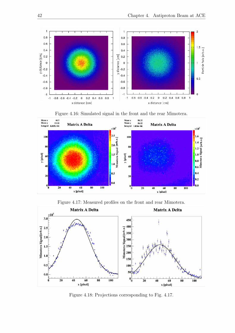
It is also possible to not only direct the beam to the center of the Mimotera, butfurthermore to align the experimental table to the beam. For this purpose, a secondMimotera has been placed approximately 50 cm behind the first one. The watertank in the middle is removed and the beam travels through air. Simulations withFLUKA have shown that despite straggling caused by the first Mimotera and the50 cm of air in between the two detectors, it should still be possible to observe afairly good beam profile, and thus to verify the alignment, as can be seen in Fig 4.16
The profiles that were obtained on the Mimotera in front of and behind the experi-ment respectively, are shown in Fig. 4.17, along with their corresponding projectionsin Fig 4.18. The results agree very well with the simulations and it is easily possibleto determine the center of the beam profile on the second Mimotera. In the caseillustrated, the mean value of the distribution differs only by about 4 pixels in x-and 3 pixels in y-direction over the range of 50 cm, which corresponds to an angleof arctan[3 × 153µm/50 cm] = 0.056 degrees. The rear Mimotera is also mountedon an adjustable holder, such that it can be moved to achieve an image of the beamcentered on the detector. Afterwards the Mimotera chip is removed from the holder,to allow a laser beam to be aligned to the center of the front and rear Mimotera.Subsequently, the water tank is adjusted to be precisely in line with the laser and,thus also with the antiproton beam.
42 Chapter 4. Antiproton Beam at ACE
Figure 4.16: Simulated signal in the front and the rear Mimotera.
Figure 4.17: Measured profiles on the front and rear Mimotera.
Figure 4.18: Projections corresponding to Fig. 4.17.
5 Ion Beams at HIT
Having demonstrated the suitability of the Mimotera for monitoring antiprotonbeams, which may be used for cancer treatment only in the not-so-near future, if atall, it is tempting to test the chip also for more conventional ion beams. The mostcommonly used hadrons for cancer therapy are protons and carbon ions. Both areapplied at the Heidelberg Ion-Beam Therapy Center (HIT), where the experimentsdescribed below have been carried out. The irradiations took place in the qualityassurance room of the facility, during the breaks in between the patient treatments.
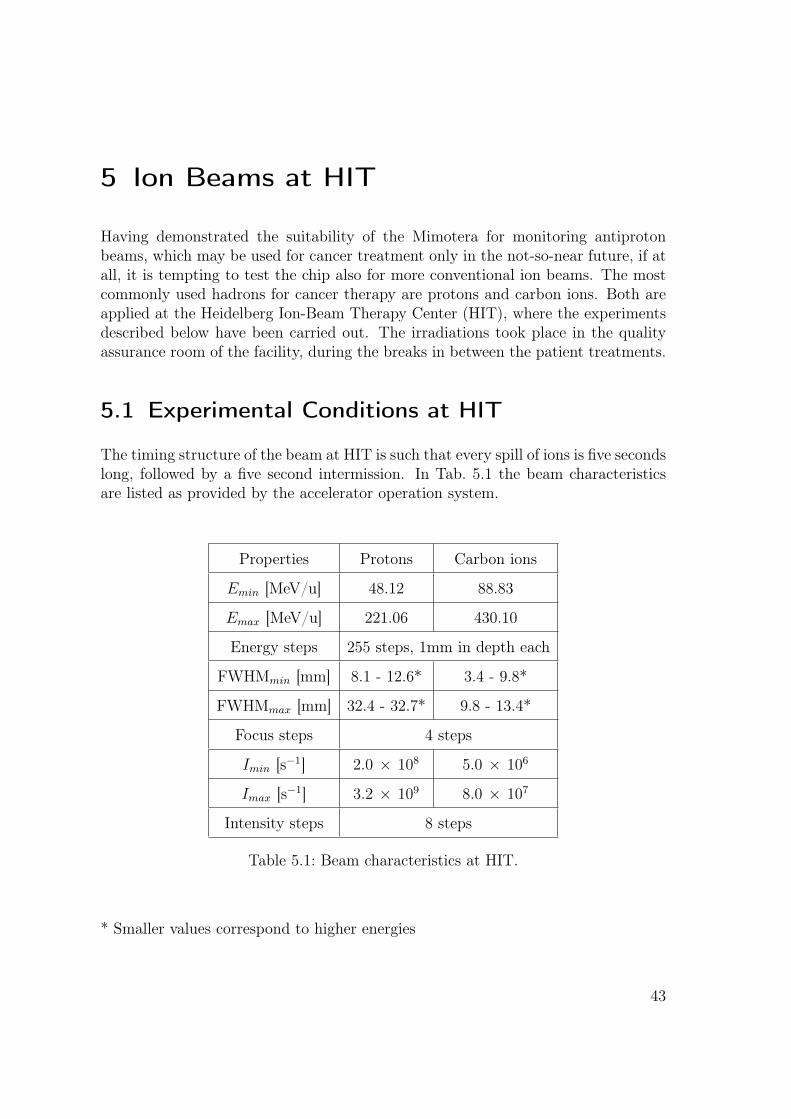
5.1 Experimental Conditions at HIT
The timing structure of the beam at HIT is such that every spill of ions is five secondslong, followed by a five second intermission. In Tab. 5.1 the beam characteristicsare listed as provided by the accelerator operation system.
Properties Protons Carbon ions
Emin [MeV/u] 48.12 88.83
Emax [MeV/u] 221.06 430.10
Energy steps 255 steps, 1mm in depth each
FWHMmin [mm] 8.1 - 12.6* 3.4 - 9.8*
FWHMmax [mm] 32.4 - 32.7* 9.8 - 13.4*
Focus steps 4 steps
Imin [s−1] 2.0 × 10⁸ 5.0 × 10⁶
Imax [s−1] 3.2 × 10⁹ 8.0 × 10⁷
Intensity steps 8 steps
Table 5.1: Beam characteristics at HIT.
* Smaller values correspond to higher energies
43
44 Chapter 5. Ion Beams at HIT
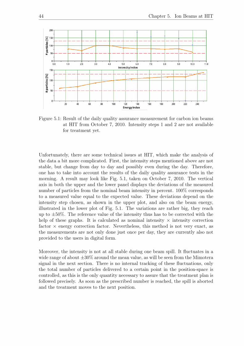
Figure 5.1: Result of the daily quality assurance measurement for carbon ion beamsat HIT from October 7, 2010. Intensity steps 1 and 2 are not availablefor treatment yet.
Unfortunately, there are some technical issues at HIT, which make the analysis ofthe data a bit more complicated. First, the intensity steps mentioned above are notstable, but change from day to day and possibly even during the day. Therefore,one has to take into account the results of the daily quality assurance tests in themorning. A result may look like Fig. 5.1, taken on October 7, 2010. The verticalaxis in both the upper and the lower panel displays the deviations of the measurednumber of particles from the nominal beam intensity in percent. 100% correspondsto a measured value equal to the expected value. These deviations depend on theintensity step chosen, as shown in the upper plot, and also on the beam energy,illustrated in the lower plot of Fig. 5.1. The variations are rather big, they reachup to ±50%. The reference value of the intensity thus has to be corrected with thehelp of these graphs. It is calculated as nominal intensity × intensity correctionfactor × energy correction factor. Nevertheless, this method is not very exact, asthe measurements are not only done just once per day, they are currently also notprovided to the users in digital form.
Moreover, the intensity is not at all stable during one beam spill. It fluctuates in awide range of about ±30% around the mean value, as will be seen from the Mimoterasignal in the next section. There is no internal tracking of these fluctuations, onlythe total number of particles delivered to a certain point in the position-space iscontrolled, as this is the only quantity necessary to assure that the treatment plan isfollowed precisely. As soon as the prescribed number is reached, the spill is abortedand the treatment moves to the next position.
5.2. Carbon Ions 45
5.2 Carbon Ions
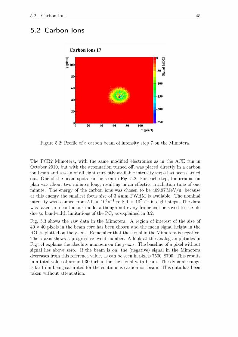
Figure 5.2: Profile of a carbon beam of intensity step 7 on the Mimotera.
The PCB2 Mimotera, with the same modified electronics as in the ACE run inOctober 2010, but with the attenuation turned off, was placed directly in a carbonion beam and a scan of all eight currently available intensity steps has been carriedout. One of the beam spots can be seen in Fig. 5.2. For each step, the irradiationplan was about two minutes long, resulting in an effective irradiation time of oneminute. The energy of the carbon ions was chosen to be 409.97 MeV/u, becauseat this energy the smallest focus size of 3.4 mm FWHM is available. The nominalintensity was scanned from 5.0 × 10⁶ s−1 to 8.0 × 10⁷ s−1 in eight steps. The datawas taken in a continuous mode, although not every frame can be saved to the filedue to bandwidth limitations of the PC, as explained in 3.2.
Fig. 5.3 shows the raw data in the Mimotera. A region of interest of the size of40× 40 pixels in the beam core has been chosen and the mean signal height in theROI is plotted on the y-axis. Remember that the signal in the Mimotera is negative.The x-axis shows a progressive event number. A look at the analog amplitudes inFig 5.4 explains the absolute numbers on the y-axis: The baseline of a pixel withoutsignal lies above zero. If the beam is on, the (negative) signal in the Mimoteradecreases from this referenca value, as can be seen in pixels 7500–8700. This resultsin a total value of around 300 arb.u. for the signal with beam. The dynamic rangeis far from being saturated for the continuous carbon ion beam. This data has beentaken without attenuation.
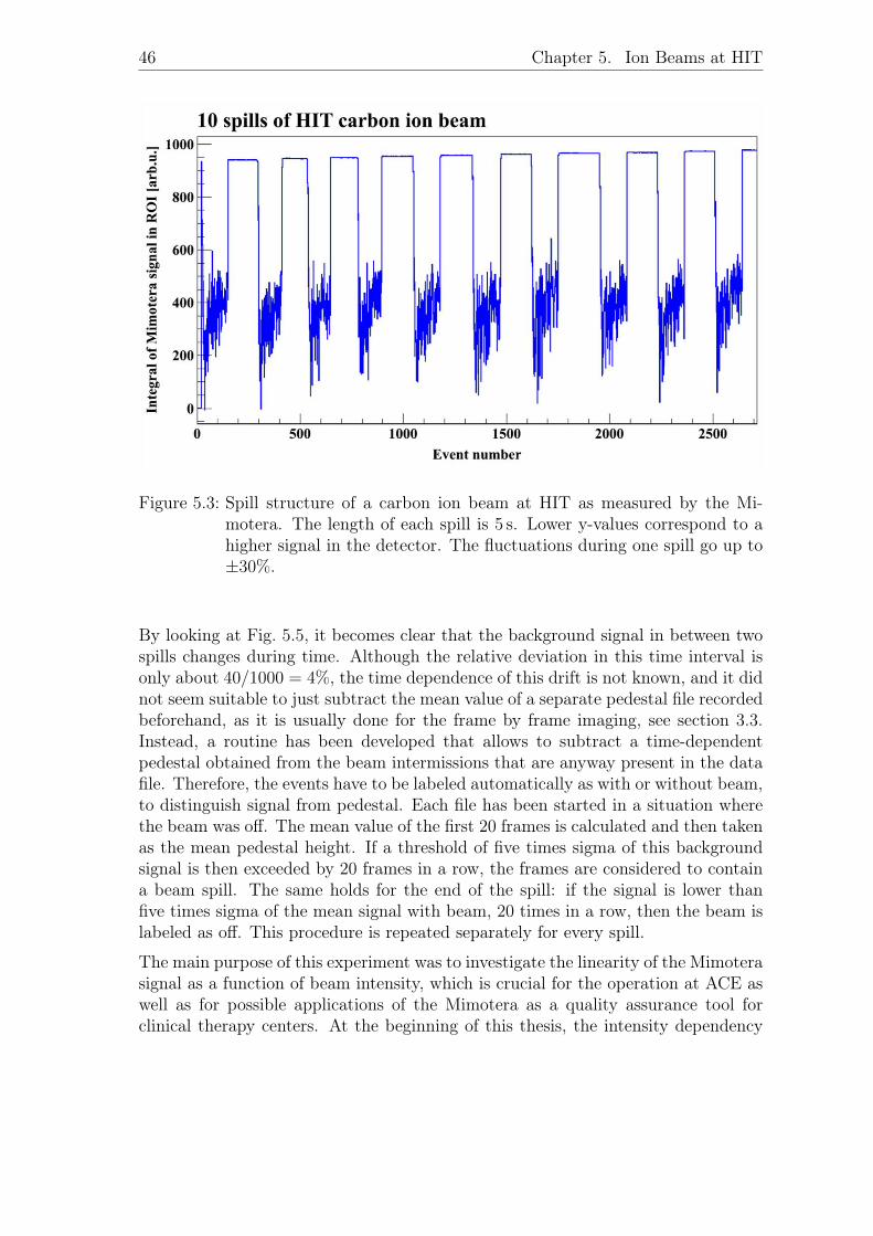
46 Chapter 5. Ion Beams at HIT
Figure 5.3: Spill structure of a carbon ion beam at HIT as measured by the Mi-motera. The length of each spill is 5 s. Lower y-values correspond to ahigher signal in the detector. The fluctuations during one spill go up to±30%.
By looking at Fig. 5.5, it becomes clear that the background signal in between twospills changes during time. Although the relative deviation in this time interval isonly about 40/1000 = 4%, the time dependence of this drift is not known, and it didnot seem suitable to just subtract the mean value of a separate pedestal file recordedbeforehand, as it is usually done for the frame by frame imaging, see section 3.3.Instead, a routine has been developed that allows to subtract a time-dependentpedestal obtained from the beam intermissions that are anyway present in the datafile. Therefore, the events have to be labeled automatically as with or without beam,to distinguish signal from pedestal. Each file has been started in a situation wherethe beam was off. The mean value of the first 20 frames is calculated and then takenas the mean pedestal height. If a threshold of five times sigma of this backgroundsignal is then exceeded by 20 frames in a row, the frames are considered to containa beam spill. The same holds for the end of the spill: if the signal is lower thanfive times sigma of the mean signal with beam, 20 times in a row, then the beam islabeled as off. This procedure is repeated separately for every spill.
The main purpose of this experiment was to investigate the linearity of the Mimoterasignal as a function of beam intensity, which is crucial for the operation at ACE aswell as for possible applications of the Mimotera as a quality assurance tool forclinical therapy centers. At the beginning of this thesis, the intensity dependency
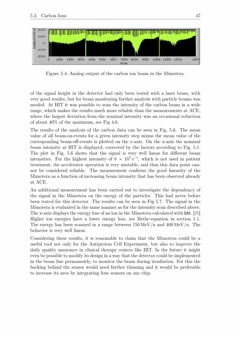
5.2. Carbon Ions 47
Figure 5.4: Analog output of the carbon ion beam in the Mimotera.
of the signal height in the detector had only been tested with a laser beam, withvery good results, but for beam monitoring further analysis with particle beams wasneeded. At HIT it was possible to scan the intensity of the carbon beam in a widerange, which makes the results much more reliable than the measurements at ACE,where the largest deviation from the nominal intensity was an occasional reductionof about 40% of the maximum, see Fig 4.6.
The results of the analysis of the carbon data can be seen in Fig. 5.6. The meanvalue of all beam-on-events for a given intensity step minus the mean value of thecorresponding beam-off-events is plotted on the y-axis. On the x-axis the nominalbeam intensity at HIT is displayed, corrected by the factors according to Fig. 5.1.The plot in Fig. 5.6 shows that the signal is very well linear for different beamintensities. For the highest intensity of 8 × 10⁷ s−1, which is not used in patienttreatment, the accelerator operation is very unstable, and thus this data point can-not be considered reliable. The measurement confirms the good linearity of theMimotera as a function of increasing beam intensity that has been observed alreadyat ACE.
An additional measurement has been carried out to investigate the dependency ofthe signal in the Mimotera on the energy of the particles. This had never beforebeen tested for this detector. The results can be seen in Fig 5.7. The signal in theMimotera is evaluated in the same manner as for the intensity scan described above.The x-axis displays the energy loss of an ion in the Mimotera calculated with bbt. [25]Higher ion energies have a lower energy loss, see Bethe-equation in section 1.1.The energy has been scanned in a range between 150 MeV/n and 400 MeV/n. Thebehavior is very well linear.
Considering these results, it is reasonable to claim that the Mimotera could be auseful tool not only for the Antiproton Cell Experiment, but also to improve thedaily quality assurance in clinical therapy centers like HIT. In the future it mighteven be possible to modify its design in a way that the detector could be implementedin the beam line permanently, to monitor the beam during irradiation. For this thebacking behind the sensor would need further thinning and it would be preferableto increase its area by integrating four sensors on one chip.
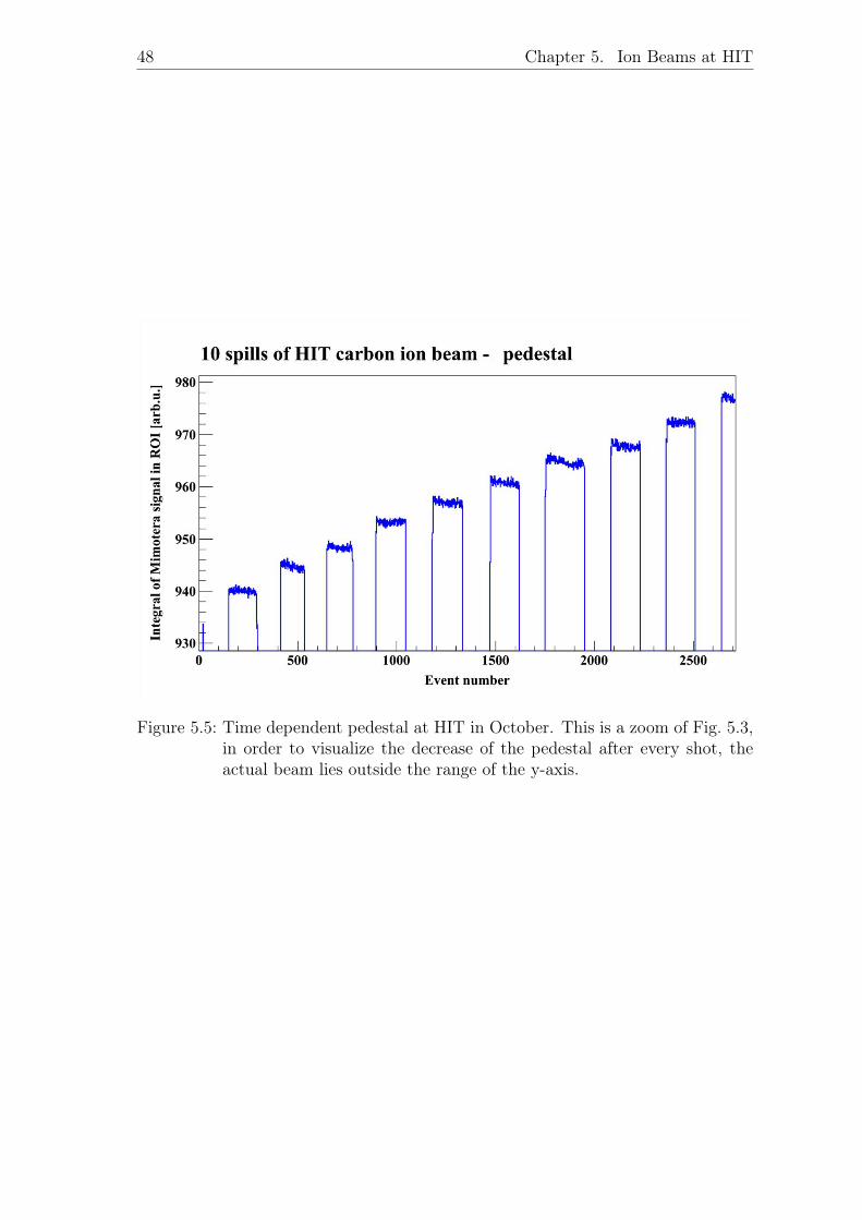
48 Chapter 5. Ion Beams at HIT
Figure 5.5: Time dependent pedestal at HIT in October. This is a zoom of Fig. 5.3,in order to visualize the decrease of the pedestal after every shot, theactual beam lies outside the range of the y-axis.
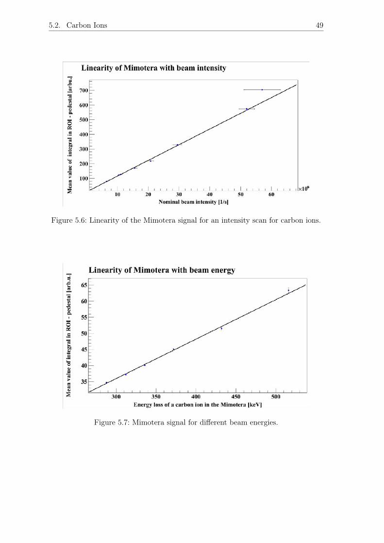
5.2. Carbon Ions 49
Figure 5.6: Linearity of the Mimotera signal for an intensity scan for carbon ions.
Figure 5.7: Mimotera signal for different beam energies.
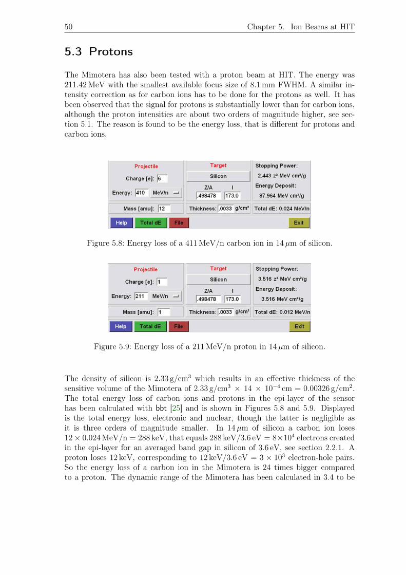
50 Chapter 5. Ion Beams at HIT
5.3 Protons
The Mimotera has also been tested with a proton beam at HIT. The energy was211.42 MeV with the smallest available focus size of 8.1 mm FWHM. A similar in-tensity correction as for carbon ions has to be done for the protons as well. It hasbeen observed that the signal for protons is substantially lower than for carbon ions,although the proton intensities are about two orders of magnitude higher, see sec-tion 5.1. The reason is found to be the energy loss, that is different for protons andcarbon ions.
Figure 5.8: Energy loss of a 411 MeV/n carbon ion in 14µm of silicon.
Figure 5.9: Energy loss of a 211 MeV/n proton in 14µm of silicon.
The density of silicon is 2.33 g/cm3 which results in an effective thickness of thesensitive volume of the Mimotera of 2.33 g/cm3 × 14 × 10−4 cm = 0.00326 g/cm2.The total energy loss of carbon ions and protons in the epi-layer of the sensorhas been calculated with bbt [25] and is shown in Figures 5.8 and 5.9. Displayedis the total energy loss, electronic and nuclear, though the latter is negligible asit is three orders of magnitude smaller. In 14µm of silicon a carbon ion loses12× 0.024 MeV/n = 288 keV, that equals 288 keV/3.6 eV = 8×10⁴ electrons createdin the epi-layer for an averaged band gap in silicon of 3.6 eV, see section 2.2.1. Aproton loses 12 keV, corresponding to 12 keV/3.6 eV = 3 × 10³ electron-hole pairs.So the energy loss of a carbon ion in the Mimotera is 24 times bigger comparedto a proton. The dynamic range of the Mimotera has been calculated in 3.4 to be

5.3. Protons 51
5× 10³ to 6× 10⁶ electrons per pixel per frame. Therefore, the energy deposition ofa 211 MeV proton is not big enough to be detected as a signal.
Unfortunately, it was not possible to do measurements for lower proton energiesat HIT, where the energy deposition would have been higher, because the minimalfocus size of the beam increases rapidly with decreasing energy, resulting for examplein a minimum focus of 32.4 mm FWHM for 50 MeV protons. As the Mimotera isonly 17× 17 mm large, it appeared not useful to apply these conditions.

6 Open Questions and Summary
6.1 Radiation Damage
An effect that is not yet entirely investigated for the Mimotera is the influence ofion irradiation on the detector response. The variety of temporal and eventuallypermanent modifications occurring during the monitoring of protons, antiprotonsand carbon ions will in the following be referred to as radiation damage. The maineffect caused by the irradiation of a crystal lattice with nuclei is the displacementof atoms in the lattice, leading to interstitials, which are atoms in places in betweentwo lattice points, and vacancies, which are empty lattice points. These have twoconsequences: They act as so called generation-recombination centers, which meansthey can capture and emit electrons and holes, leading to an increased leakagecurrent in the space charge region. Moreover, they act as trapping centers for thesignal charge carriers, causing a delay of the detection, and a decrease of the signal.See [24] for more details.
Ion beams at HIT
In Fig. 6.1, the analog output of the Mimotera immediately after two different days ofirradiations with protons and carbon ions at HIT can be seen. The total irradiationtime was about two hours for all runs, the beam intensity has been scanned to studythe linearity of the detector response. For the first test on May 20, 2010 there is aclear increase of the background signal at the same position on the sensor where thecarbon ion beam had been placed. This reaches up to the level that hit pixels areeven saturated when using the unattenuated configuration of the Mimotera, as canbe seen in the upper part of Fig. 6.1. Also, the position of the proton beam, whichhad been shifted with respect to the carbon beam is visible after the irradiation.
This impression can be quantified by analyzing the integral of the signal in a regionof interest at the beam position, as explained in section 5.2. The result in Fig. 6.2shows the absolute value of the pedestal, i.e. the signal height per pixel that decreasesafter every spill of carbon ions. This corresponds to an increase of the background, asthe signal in the Mimotera is negative. The cause for this are probably generation-recombination centers in the silicon crystal, as mentioned above. The defects inthe crystal lattice are electrically active and cause a capture and re-emittance ofelectrons that is visible in the analog output.
53
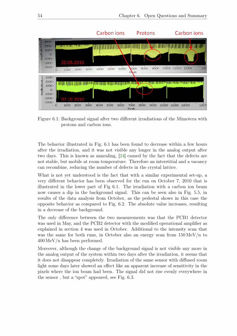
54 Chapter 6. Open Questions and Summary
Figure 6.1: Background signal after two different irradiations of the Mimotera withprotons and carbon ions.
The behavior illustrated in Fig. 6.1 has been found to decrease within a few hoursafter the irradiation, and it was not visible any longer in the analog output aftertwo days. This is known as annealing, [24] caused by the fact that the defects arenot stable, but mobile at room temperature. Therefore an interstitial and a vacancycan recombine, reducing the number of defects in the crystal lattice.
What is not yet understood is the fact that with a similar experimental set-up, avery different behavior has been observed for the run on October 7, 2010 that isillustrated in the lower part of Fig 6.1. The irradiation with a carbon ion beamnow causes a dip in the background signal. This can be seen also in Fig. 5.5, inresults of the data analysis from October, as the pedestal shows in this case theopposite behavior as compared to Fig. 6.2. The absolute value increases, resultingin a decrease of the background.
The only difference between the two measurements was that the PCB1 detectorwas used in May, and the PCB2 detector with the modified operational amplifier asexplained in section 4 was used in October. Additional to the intensity scan thatwas the same for both runs, in October also an energy scan from 150 MeV/n to400 MeV/n has been performed.
Moreover, although the change of the background signal is not visible any more inthe analog output of the system within two days after the irradiation, it seems thatit does not disappear completely. Irradiation of the same sensor with diffused roomlight some days later showed an effect like an apparent increase of sensitivity in thepixels where the ion beam had been. The signal did not rise evenly everywhere inthe sensor , but a “spot” appeared, see Fig. 6.3.
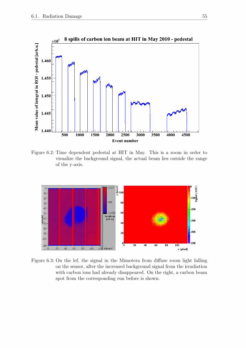
6.1. Radiation Damage 55
Figure 6.2: Time dependent pedestal at HIT in May. This is a zoom in order tovisualize the background signal, the actual beam lies outside the rangeof the y-axis.
Figure 6.3: On the lef, the signal in the Mimotera from diffuse room light fallingon the sensor, after the increased background signal from the irradiationwith carbon ions had already disappeared. On the right, a carbon beamspot from the corresponding run before is shown.
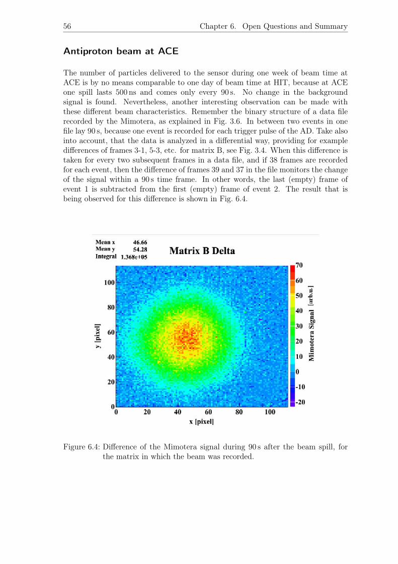
56 Chapter 6. Open Questions and Summary
Antiproton beam at ACE
The number of particles delivered to the sensor during one week of beam time atACE is by no means comparable to one day of beam time at HIT, because at ACEone spill lasts 500 ns and comes only every 90 s. No change in the backgroundsignal is found. Nevertheless, another interesting observation can be made withthese different beam characteristics. Remember the binary structure of a data filerecorded by the Mimotera, as explained in Fig. 3.6. In between two events in onefile lay 90 s, because one event is recorded for each trigger pulse of the AD. Take alsointo account, that the data is analyzed in a differential way, providing for exampledifferences of frames 3-1, 5-3, etc. for matrix B, see Fig. 3.4. When this difference istaken for every two subsequent frames in a data file, and if 38 frames are recordedfor each event, then the difference of frames 39 and 37 in the file monitors the changeof the signal within a 90 s time frame. In other words, the last (empty) frame ofevent 1 is subtracted from the first (empty) frame of event 2. The result that isbeing observed for this difference is shown in Fig. 6.4.
Figure 6.4: Difference of the Mimotera signal during 90 s after the beam spill, forthe matrix in which the beam was recorded.
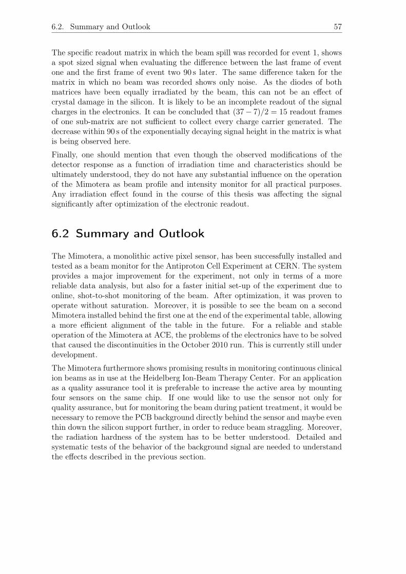
6.2. Summary and Outlook 57
The specific readout matrix in which the beam spill was recorded for event 1, showsa spot sized signal when evaluating the difference between the last frame of eventone and the first frame of event two 90 s later. The same difference taken for thematrix in which no beam was recorded shows only noise. As the diodes of bothmatrices have been equally irradiated by the beam, this can not be an effect ofcrystal damage in the silicon. It is likely to be an incomplete readout of the signalcharges in the electronics. It can be concluded that (37− 7)/2 = 15 readout framesof one sub-matrix are not sufficient to collect every charge carrier generated. Thedecrease within 90 s of the exponentially decaying signal height in the matrix is whatis being observed here.
Finally, one should mention that even though the observed modifications of thedetector response as a function of irradiation time and characteristics should beultimately understood, they do not have any substantial influence on the operationof the Mimotera as beam profile and intensity monitor for all practical purposes.Any irradiation effect found in the course of this thesis was affecting the signalsignificantly after optimization of the electronic readout.
6.2 Summary and Outlook
The Mimotera, a monolithic active pixel sensor, has been successfully installed andtested as a beam monitor for the Antiproton Cell Experiment at CERN. The systemprovides a major improvement for the experiment, not only in terms of a morereliable data analysis, but also for a faster initial set-up of the experiment due toonline, shot-to-shot monitoring of the beam. After optimization, it was proven tooperate without saturation. Moreover, it is possible to see the beam on a secondMimotera installed behind the first one at the end of the experimental table, allowinga more efficient alignment of the table in the future. For a reliable and stableoperation of the Mimotera at ACE, the problems of the electronics have to be solvedthat caused the discontinuities in the October 2010 run. This is currently still underdevelopment.
The Mimotera furthermore shows promising results in monitoring continuous clinicalion beams as in use at the Heidelberg Ion-Beam Therapy Center. For an applicationas a quality assurance tool it is preferable to increase the active area by mountingfour sensors on the same chip. If one would like to use the sensor not only forquality assurance, but for monitoring the beam during patient treatment, it would benecessary to remove the PCB background directly behind the sensor and maybe eventhin down the silicon support further, in order to reduce beam straggling. Moreover,the radiation hardness of the system has to be better understood. Detailed andsystematic tests of the behavior of the background signal are needed to understandthe effects described in the previous section.


Appendix
59


A Mimotera Manual for ACE
Handle with care!
• The sensor must never be touched with anything! There are verythin wires connecting the PCB background to the sensor, which can be easilyunbonded. If the chip has to be unmounted from the holder for some reason,touch only the PCB and only on the edges. Be extremely careful with thescrewdriver, side-slipping may cause irreparable damage.
• When changing cell samples in the water tank, please, make sure that no liquidgets in contact with the sensor, the data acquisition board or the laptop.
• The whole system is sensitive to motion. Shocks or moving the system whilerunning might cause a crash of the data acquisition. Do not stress the greencable, it is very sensitive and has to hang loose all the time.
If there is a crash of the program, do the following:
1. Close LabView
2. Close CyConsle
3. Turn off the power supply and wait a few seconds.
4. Turn it back on and continue with “Setting up the system” below.
A.1 Setting up the system
Installation of the DAQ Software
1. Install LVRuntimeEng.exe
2. Install Cypress USB console
3. Copy the file CyUSB.inf (in the Cypress installer folder) in C:/programs/cypress/USBDevStudio/Driver
4. Connect the system to the PC. (See also next paragraph) Turn on the powersupply. The first time, Windows asks for drivers. Select “No, not this time”in the installation wizard. Then chose the path of the cypress’ drivers folderas above.
61
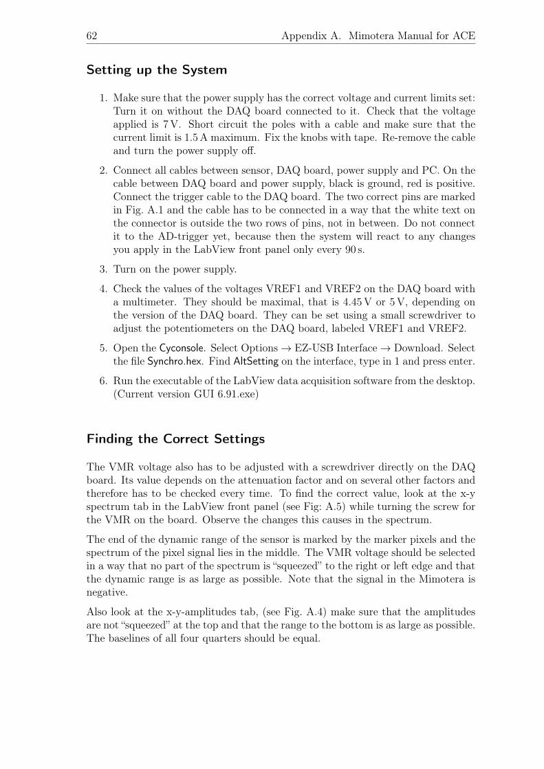
62 Appendix A. Mimotera Manual for ACE
Setting up the System
1. Make sure that the power supply has the correct voltage and current limits set:Turn it on without the DAQ board connected to it. Check that the voltageapplied is 7 V. Short circuit the poles with a cable and make sure that thecurrent limit is 1.5 A maximum. Fix the knobs with tape. Re-remove the cableand turn the power supply off.
2. Connect all cables between sensor, DAQ board, power supply and PC. On thecable between DAQ board and power supply, black is ground, red is positive.Connect the trigger cable to the DAQ board. The two correct pins are markedin Fig. A.1 and the cable has to be connected in a way that the white text onthe connector is outside the two rows of pins, not in between. Do not connectit to the AD-trigger yet, because then the system will react to any changesyou apply in the LabView front panel only every 90 s.
3. Turn on the power supply.
4. Check the values of the voltages VREF1 and VREF2 on the DAQ board witha multimeter. They should be maximal, that is 4.45 V or 5 V, depending onthe version of the DAQ board. They can be set using a small screwdriver toadjust the potentiometers on the DAQ board, labeled VREF1 and VREF2.
5. Open the Cyconsole. Select Options→ EZ-USB Interface→ Download. Selectthe file Synchro.hex. Find AltSetting on the interface, type in 1 and press enter.
6. Run the executable of the LabView data acquisition software from the desktop.(Current version GUI 6.91.exe)
Finding the Correct Settings
The VMR voltage also has to be adjusted with a screwdriver directly on the DAQboard. Its value depends on the attenuation factor and on several other factors andtherefore has to be checked every time. To find the correct value, look at the x-yspectrum tab in the LabView front panel (see Fig: A.5) while turning the screw forthe VMR on the board. Observe the changes this causes in the spectrum.
The end of the dynamic range of the sensor is marked by the marker pixels and thespectrum of the pixel signal lies in the middle. The VMR voltage should be selectedin a way that no part of the spectrum is “squeezed” to the right or left edge and thatthe dynamic range is as large as possible. Note that the signal in the Mimotera isnegative.
Also look at the x-y-amplitudes tab, (see Fig. A.4) make sure that the amplitudesare not “squeezed” at the top and that the range to the bottom is as large as possible.The baselines of all four quarters should be equal.
A.2. Taking Data 63
Figure A.1: The two pins that have to be used for triggering the DAQ board.
A.2 Taking Data
1. Enter the correct settings of all parameters on the LabView front panel thatcan be seen in Fig. A.2.
• Check Mkoff and Mkoff2 in order to avoid influences of the digital outputson the analog signal.
• Uncheck SO.
• Check PCB Hybrid if a PCB system is in use.
• Uncheck AT, unless you would like to attenuate the signal height by afactor of about five.
• Select Post-reset pulse = 6 in order to have the marker pixels in the rightpositions.
• Select Reset pulse width = 3
• Select ADC clock delay = 1
• Select the desired number of frames to save after each trigger. (“aftertrig. fr. amount”) and before each trigger. (“after trig. fr. amount”).The sum of both can be maximum 38. If you save for example 6 framesbefore each trigger, it means that the beam spill is always contained inframe number 7.

64 Appendix A. Mimotera Manual for ACE
• Press the button const/trigger in a way that it is dark green, not lightgreen.
• Select ADC-CLK = 2.5 MHz
Afterwards, click “Send Parameters”, preferably two or three times to be surethe input was accepted.
2. Now connect the cable to the AD trigger. Everything else can then be doneremotely from outside the zone.
3. Enter how many events you would like to save (“no. of events to store”,Fig. A.2). This is the number of events that will be saved to one data file.At ACE, each event corresponds to one trigger pulse of the AD, one event issaved every 90 s. To obtain the number of frames that are stored, multiplythe number of events by [(after trig. fr. amount) + (before trig. fr. amount)].Note that one event consisting of 38 frames needs roughly 2 MB and that adata file must not exceed 2 GB.
4. Enter the full path of the file including the extension .dat at the interface, seeFig. A.2. If you do not change the filename in between two runs, the first filewill not be overwritten but the data is attached to the first file.
5. Click “save to file”. As soon as the next trigger pulse arrives, the green lightwill light up and “no of events to store” will start counting down from thevalue you entered to zero. If you wish to stop the data taking earlier, press“stop saving”. In this case the number will immediately jump to 1 and the filewill be finished after the next trigger pulse that arrives.
To see the beam online on the front panel, make sure that the following adjustmentsare correct:
• On the X-Y-Subtract tab on the right in Fig. A.2, the difference has to betaken between the frame that contains the beam spill and the previous one. If6 frames are saved before each trigger, this has to be relative frame number 7minus 6.
• The beam can be in matrix A or in matrix B. If you do not see anything, trychanging “matrix to subtract” from A(x)–A(y) to B(x)–B(y) in the same tab.
Now you should be able to see the beam in the X-Y-Subtract tab as in Fig. A.6.
Looking at the tab Beam on-line imaging in Fig A.7, in order to see the beam, makesure that:
• No. to sum up for display is 1. Otherwise several events are summed up untilyou can see the beam.
• Analog to the X-Y-Subtract, change between matrix A and B in case the beamwas recorded in the other matrix.
When an adjustment of the beam is necessary, consider the following: The pictureof the beam that is visible on the interface is what you see when you stand behind
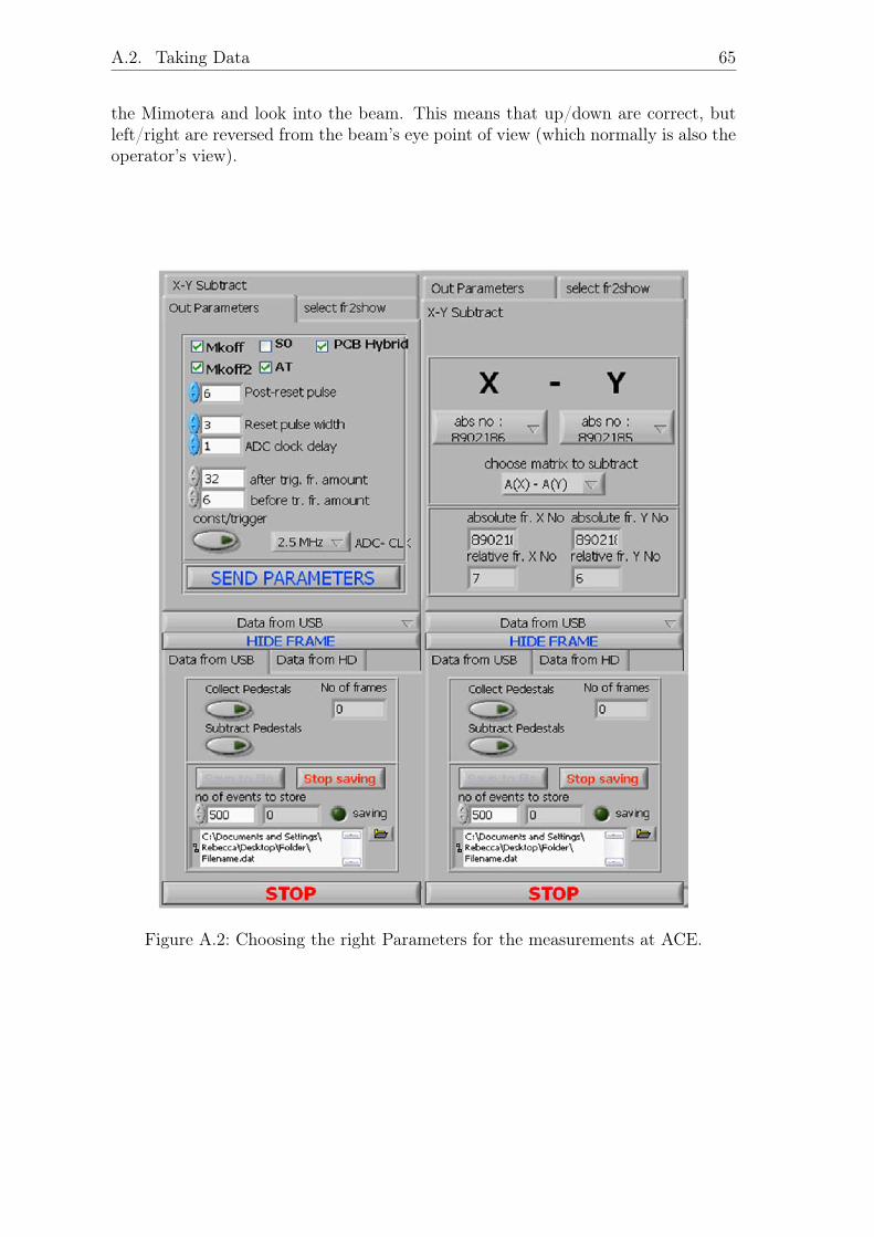
A.2. Taking Data 65
the Mimotera and look into the beam. This means that up/down are correct, butleft/right are reversed from the beam’s eye point of view (which normally is also theoperator’s view).
Figure A.2: Choosing the right Parameters for the measurements at ACE.
66 Appendix A. Mimotera Manual for ACE
Figure A.3: Selected AB frame in LabView.
Figure A.4: X–Y–Amplitudes in LabView.
Figure A.5: X–Y–Spectrum in LabView.
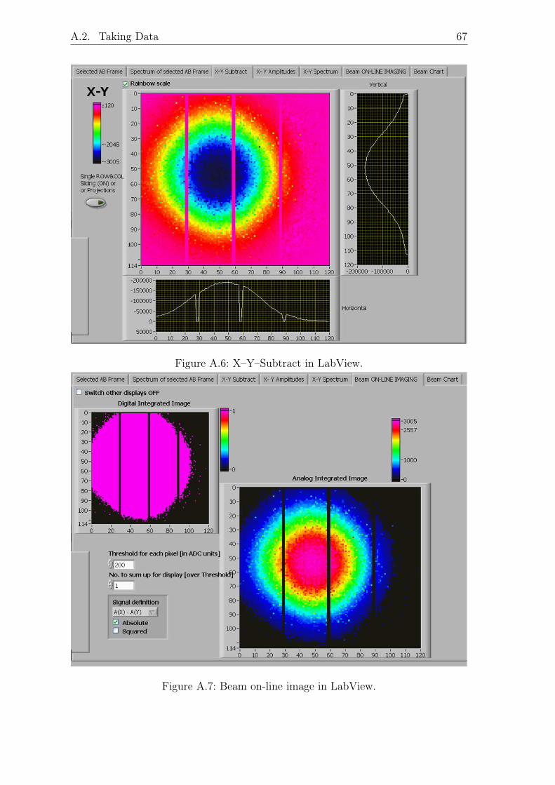
A.2. Taking Data 67
Figure A.6: X–Y–Subtract in LabView.
Figure A.7: Beam on-line image in LabView.


B Bibliography
[1] Particle Data Group: Review of Particle Physics. University of California,2010.
[2] G. Kraft: Tumor therapy with heavy charged particles. Prog. Part. Nucl. Phys.45, 2000.
[3] http://ptcog.web.psi.ch/
[4] M. Henley, A. Garcia: Subatomic Physics. World Scientific Publishing Co. Pre.Ltd., Singapore. 3. edition, 2007.
[5] W. H. Bragg and R. Kleemann: On the Ionization Curves of Radium. Phil.Mag. 8, 1963.
[6] S. Sellner: Real-Time Imaging of the Annihilation Vertex Distributions forAntiprotons Stopping in Biological Targets. Diploma thesis, 2010.
[7] T. E. Kalogeropoulos, R. Muratore: Antiprotons for Imaging and Therapy.Nucl. Inst. Meth. B40/41, 1989.
[8] M. Holzscheiter et al.: The Biological Effectiveness of Antiproton Irradiation.Radiotherapy & Oncology 81, 2006.
[9] S. Maury: The Antiproton Decelerator: AD. Hyperfine Interact. 109, 1997.
[10] B. G. Wouters, G. K. Lam, U. Oelfke, K. Gardey, R. E. Durand, L. D. Skars-gard: Measurements of relative biological effectiveness of the 70 MeV protonbeam at TRIUMF using Chinese hamster V79 cells and the high-precision cellsorter assay. Radiat. Res. 146, 1996.
[11] http://www.tera.it/ise.cgi
[12] http://www.bergoz.com/index.php?option=com_content&view=article&id=14&Itemid=17
[13] M. Martisikova, B. Ackermann, S. Klemm, O. Jäkel: Use of Gafchromic EBTfilms in heavy ion therapy. Nucl. Inst. Methods Phys. Res. A 591, 2008.
[14] S. M. Sze: Physics of semiconductor devices. Wiley, New York. 3. edition, 2007.
[15] S. Hunklinger: Festkörperphysik. Oldenbourg Wissenschaftsverlag, München.1. edition, 2007.
69
70 B Bibliography
[16] P.Riedler: Lecture on Silicon Pixel detectors. Geneva, 2006/2007.
[17] http://www-m2.ma.tum.de/homepages/gilg/notesd/Vorl_S_K1.pdf
[18] http://en.wikipedia.org/wiki/Scintillator
[19] L.Bandano: Developpement d’un moniteur de faisceau innovant pour la mesureen temps reel des faisceaux utilises en hadron therapie. PhD thesis, 2005.
[20] http://root.cern.ch/drupal/
[21] V. Radeka: Low-noise techniques in detectors. Ann. Rev. Nucl. Part. Sci. 38,1988.
[22] C. Brusasco, B. Voss, D. Schardt, M. Krämer, G. Kraft: A dosimetry system forfast measurement of 3D depth-dose profiles in charged-particle tumor therapywith scanning techniques. Nucl. Inst. Methods Phys. Res. B 168, 2000.
[23] P. Riedler, J. Rochet, A. Rudge, M. Doser, R. Landua: Performance of ultra-thin silicon detectors in a 5 MeV antiproton beam. Nucl. Inst. Methods Phys.Res. A 478, 2002.
[24] G. Lutz: Semiconductor Radiation Detectors. Springer-Verlag, Berlin Heidel-berg, 2007
[25] http://www.sgeier.net/tools/bbt.html
Acknowledgments
At this point I would like to thank everybody who supported my work during thelast year, and who contributed to this thesis in any way:
Michael Holzscheiter, for always giving good answers and posing the right questions,and for believing in me in moments I didn’t.
Joachim Ullrich, for having helpful suggestions and questions, and for improving theresult of this thesis.
Oliver Jäkel, for always supporting my work and making the measurements at theHeidelberg Ion-Beam Therapy Center possible.
Massimo Caccia, for enabling this work in the first place, by providing the detectoralong with a lot of first-hand advice and many emails; Loretta Negrini, for being ofgreat help in measuring and analyzing data; and everybody else from this group atthe Università dell’ Insubria in Como, Italy.
The members of the QUASAR group at the Max-Planck-Institute for Nuclear Physics,Heidelberg, Germany; particularly Carsten Welsch, for his support and ideas.
The members of the E040-9 group at the German Cancer Research Center, Heidel-berg, Germany, for good collaboration.
Stefan Sellner, for processing the simulations and for arbitrating between me andmy computer.
Kirsten Vincke, Jana Schnieders, and Dennis Kütemeier, for finding hopefully everymistake I made.
Someone special, for never stopping to believe in me.
71


Erklärung:
Ich versichere, dass ich diese Arbeit selbstständig verfasst habe und keine anderenals die angegebenen Quellen und Hilfsmittel benutzt habe.
Heidelberg, den 1. Dezember 2010 . . . . . . . . . . . . . . . . . . . . . . . . . . . . . . .