Embed Size (px)
Citation preview
MSc Physics and Astronomy
Theoretical Physics
Master Thesis
The Replica Trick and Replica Wormholes
by
Joost Pluijmen
6044557
August 2020
60 ECTS
Research carried out between May 2019 and August 2020
Supervisor/Examiner: Examiner:
Dr. Ben Freivogel Prof. Dr. Erik Verlinde
Institute for Theoretical Physics Amsterdam (ITFA)
[ August 28, 2020 at 11:14 –]

A B S T R A C T
Stephen Hawking proposed that a black hole formed from the collapse of a pure statewould disappear after a period of evaporation. The resulting evaporated radiation,known as Hawking radiation, would then be left in a mixed state. In case this is true,information would be lost and there would be no unitary evolution from the initial purestate to a final pure state. This problem is called the ”black hole information paradox”(BHIP). If we demand unitarity, the entropy that is created during the formation andevaporation of a black hole should follow the ”Page curve” as the black hole evaporates.In this thesis, I will give an introduction to the concept of entropy and show examples ofhow we can use the ”replica trick” to calculate this entropy. The replica trick can alsobe used to calculate the entropy of evaporating Euclidean black holes with the help of”replica wormholes”. The idea is that by introducing these wormholes, the Hawkingradiation will end up in a pure state so the we can solve the BHIP. Here, we show howthese replica wormholes ensure unitarity in AdS2.
ii
[ August 28, 2020 at 11:14 –]

Tingelingeling
— Pieter H. M. Pluijmen
A C K N O W L E D G M E N T S
Many thanks to my supervisor Ben Freivogel, who helped me outstandingly with all hisadvises. Thanks to Ben, the trajectory of my thesis project has been really smooth. TheZoom-talks during the Corona pandemic where good replacements of the earlier face-to-face meetings, with the blackboard from a distance, to help me understand differenttopics. I also want to thank my girlfriend Esin, who dragged me trough the last periodof my study and who supports me in every aspect of life. Last but not least I want tothank my parents who are my oldest and dearest friends and who have had my backduring my whole studentship.
iii
[ August 28, 2020 at 11:14 –]

C O N T E N T S
1 introduction 1
2 von neumann entropy and the replica trick 4
2.1 Von Neumann Entropy . . . . . . . . . . . . . . . . . . . . . . . . . . . . . . 4
2.2 The Replica Trick . . . . . . . . . . . . . . . . . . . . . . . . . . . . . . . . . 6
2.3 Canonical Ensemble . . . . . . . . . . . . . . . . . . . . . . . . . . . . . . . 6
2.4 Example: the Harmonic Oscillator . . . . . . . . . . . . . . . . . . . . . . . 9
3 euclidean path integrals and the replica trick in quantum
mechanics 11
3.1 Propagator . . . . . . . . . . . . . . . . . . . . . . . . . . . . . . . . . . . . . 11
3.2 Euclidean Time . . . . . . . . . . . . . . . . . . . . . . . . . . . . . . . . . . 12
3.3 Free Particle . . . . . . . . . . . . . . . . . . . . . . . . . . . . . . . . . . . . 15
3.3.1 Propagator . . . . . . . . . . . . . . . . . . . . . . . . . . . . . . . . . 15
3.3.2 Replica Trick . . . . . . . . . . . . . . . . . . . . . . . . . . . . . . . 18
3.4 Harmonic Oscillator . . . . . . . . . . . . . . . . . . . . . . . . . . . . . . . 19
3.4.1 Propagator . . . . . . . . . . . . . . . . . . . . . . . . . . . . . . . . . 19
3.4.2 Replica Trick . . . . . . . . . . . . . . . . . . . . . . . . . . . . . . . 23
4 euclidean path integrals and the replica trick in free scalar
field theory 28
4.1 Propagator . . . . . . . . . . . . . . . . . . . . . . . . . . . . . . . . . . . . . 28
4.2 Euclidean Spacetime . . . . . . . . . . . . . . . . . . . . . . . . . . . . . . . 30
4.3 Massive Free Scalar Field in d-Dimensional Euclidean Spacetime . . . . . 32
4.3.1 Replica Trick . . . . . . . . . . . . . . . . . . . . . . . . . . . . . . . 36
4.4 The Cardy Formula . . . . . . . . . . . . . . . . . . . . . . . . . . . . . . . . 38
4.5 Rindler Coordinates . . . . . . . . . . . . . . . . . . . . . . . . . . . . . . . 41
4.5.1 Minkowski spacetime . . . . . . . . . . . . . . . . . . . . . . . . . . 41
4.5.2 Euclidean spacetime . . . . . . . . . . . . . . . . . . . . . . . . . . . 43
4.6 Massless Free Scalar Field in 2-dimensional Euclidean Rindler Spacetime 44
5 black hole entropy and replica wormholes 50
5.1 Black Hole Entropy and the Entropy of Hawking Radiation . . . . . . . . 50
5.1.1 Bekenstein-Hawking entropy . . . . . . . . . . . . . . . . . . . . . . 50
5.1.2 Partition function . . . . . . . . . . . . . . . . . . . . . . . . . . . . . 51
5.1.3 Effective action . . . . . . . . . . . . . . . . . . . . . . . . . . . . . . 51
5.1.4 New Rules . . . . . . . . . . . . . . . . . . . . . . . . . . . . . . . . . 52
5.2 Euclidean AdS2 . . . . . . . . . . . . . . . . . . . . . . . . . . . . . . . . . . 53
5.3 Replica Wormholes in Euclidean AdS2 . . . . . . . . . . . . . . . . . . . . . 55
5.3.1 Constructing Mn . . . . . . . . . . . . . . . . . . . . . . . . . . . . . 55
5.3.2 IdentifyingMn . . . . . . . . . . . . . . . . . . . . . . . . . . . . . . 62
5.4 Replica Trick on the Replica Manifold . . . . . . . . . . . . . . . . . . . . . 63
6 conclusions & future research 65
6.1 Conclusions . . . . . . . . . . . . . . . . . . . . . . . . . . . . . . . . . . . . 65
6.2 Future Research . . . . . . . . . . . . . . . . . . . . . . . . . . . . . . . . . . 66
a appendices 67
iv
[ August 28, 2020 at 11:14 –]

contents v
a.1 Replica Trick . . . . . . . . . . . . . . . . . . . . . . . . . . . . . . . . . . . . 67
a.2 Saddle Point Approximation . . . . . . . . . . . . . . . . . . . . . . . . . . 68
a.2.1 Quantum Mechanics . . . . . . . . . . . . . . . . . . . . . . . . . . . 68
a.2.2 Free Scalar Field Theory . . . . . . . . . . . . . . . . . . . . . . . . . 73
a.3 Direct Calculation of the Propagator of the Free Particle . . . . . . . . . . 75
a.4 Direct Calculation of the Partition Function of the Harmonic Oscillator . 76
bibliography 80
[ August 28, 2020 at 11:14 –]
1I N T R O D U C T I O N
Almost 50 years after Stephen Hawking discovered that black holes evaporate in the formof Hawking radiation [1, 2], theoretical physicists are still not sure about what happensto quantum information in and around black holes. This uncertainty is most clearlyexplained in the Black Hole Information Paradox (BHIP) [3, 4, 5].
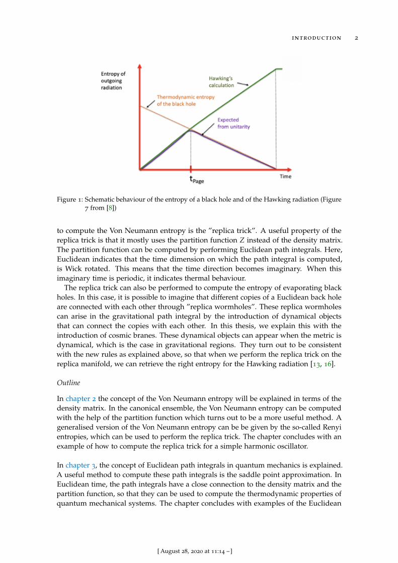
An important feature of the BHIP involves the evolution of the state of the system.This state can be represented by the density matrix ρ, which describes the possibleconfigurations of the system. The Von Neumann entropy SVN diagnoses the ”mixedness”of a state and it vanishes when ρ is in a pure state 1. An important property of the VonNeumann entropy is that it is invariant under unitary time evolution. This unitarityimplies that a state that is pure at an initial time will remain pure after a unitary timeevolution. The BHIP, however, signals that when a black hole, formed from a purestate, evaporates, the Hawking radiation will end up in a mixed state, which means thatunitarity is violated. This effect will cause the Von Neumann entropy to keep growing,whereas unitarity implies that the final density matrix should be pure so that the finalVon Neumann entropy of the Hawking radiation should decrease.
The Bekenstein-Hawking entropy, SBH = A4GN
, describes the entropy of a black holeas a thermodynamic object 2. Here, A represents the area of the horizon of the blackhole, whereas GN is the Newton constant. When a black hole evaporates, logically, SBH
decreases. This means that at some point in time, the entropy of the Hawking radiationSrad, should equal SBH. Following the work of Don Page [6, 7], we call this time thePage time tPage. Page demonstrated that the entropy should follow the Page curve. InFigure 1 we can see that the green line representing the entropy of the Hawking radiationkeeps increasing over time, whereas the orange line representing the Bekenstein-Hawkingentropy of the black hole decreases to zero. The purple line represents the Page curve andshows how the entropy of the combination of the black hole and the Hawking radiationis expected to evolve under unitary time evolution.
In a series of papers [9, 10, 11, 12, 13, 14, 15], a set of ”new rules” was developed tocalculate the entropy of evaporating black holes and of the Hawking radiation. Theserules involve a so-called ”quantum extremal surface” that is not the event horizon ofthe black hole. This surface minimises the generalised entropy Sgen which combines theBekenstein-Hawking entropy with the entropy of matter in and around the black hole.An important facet of this new concept is that it seems to be consistent with unitary timeevolution.
In this thesis, I will examine the properties of the density matrix in the context ofquantum mechanics and of free scalar field theory. As stated before, the density matrixdefines the Von Neumann entropy, but in many cases is very had to compute. A method
1In Chapters 2, 3 & 4, I will use S instead of SVN to indicate the Von Neumann entropy.2In this thesis, I will use natural units so that h = c = kB = 1.
1
[ August 28, 2020 at 11:14 –]
introduction 2
Figure 1: Schematic behaviour of the entropy of a black hole and of the Hawking radiation (Figure7 from [8])
to compute the Von Neumann entropy is the ”replica trick”. A useful property of thereplica trick is that it mostly uses the partition function Z instead of the density matrix.The partition function can be computed by performing Euclidean path integrals. Here,Euclidean indicates that the time dimension on which the path integral is computed,is Wick rotated. This means that the time direction becomes imaginary. When thisimaginary time is periodic, it indicates thermal behaviour.
The replica trick can also be performed to compute the entropy of evaporating blackholes. In this case, it is possible to imagine that different copies of a Euclidean back holeare connected with each other through ”replica wormholes”. These replica wormholescan arise in the gravitational path integral by the introduction of dynamical objectsthat can connect the copies with each other. In this thesis, we explain this with theintroduction of cosmic branes. These dynamical objects can appear when the metric isdynamical, which is the case in gravitational regions. They turn out to be consistentwith the new rules as explained above, so that when we perform the replica trick on thereplica manifold, we can retrieve the right entropy for the Hawking radiation [13, 16].
Outline
In chapter 2 the concept of the Von Neumann entropy will be explained in terms of thedensity matrix. In the canonical ensemble, the Von Neumann entropy can be computedwith the help of the partition function which turns out to be a more useful method. Ageneralised version of the Von Neumann entropy can be be given by the so-called Renyientropies, which can be used to perform the replica trick. The chapter concludes with anexample of how to compute the replica trick for a simple harmonic oscillator.
In chapter 3, the concept of Euclidean path integrals in quantum mechanics is explained.A useful method to compute these path integrals is the saddle point approximation. InEuclidean time, the path integrals have a close connection to the density matrix and thepartition function, so that they can be used to compute the thermodynamic properties ofquantum mechanical systems. The chapter concludes with examples of the Euclidean
[ August 28, 2020 at 11:14 –]

introduction 3
path integrals for the free particle and the harmonic oscillator, where for both cases, thereplica trick can be performed.
In chapter 4 the concept of Euclidean path integrals is explained for free scalar fieldtheories. Similar as with the quantum mechanical path integrals, these path integrals canbe used to compute the thermodynamic properties of field theories. The saddle pointapproximation will be used to compute the path integrals of the massive free scalar fieldin d-dimesional Minkowski spacetime. A special representation of Minkowski spacetimeis given by the Rindler metric of an uniformly accelerated observer. The last exampleinvolves the computation of the entropy of a massless free scalar field in 2-dimensionalRindler spacetime. As a bonus, this chapter provides a derivation of he Cardy formulafor 2-dimensional CFT’s.
In chapter 5 the concept of black hole entropy is explained. The generalised entropyformula seems to be insufficient to compute the right entropy for evaporating black holes,so that two ”new rules” are introduced. The introduction of n replica wormholes assaddle points in the Euclidean path integral can be used to perform the replica trick overa spacetime manifold that we constructed in AdS2.
In chapter 6 I will conclude this thesis by giving some final thoughts on the retrievedresults. Furthermore, I will give some suggestions for future research.
[ August 28, 2020 at 11:14 –]
2V O N N E U M A N N E N T R O P Y A N D T H E R E P L I C A T R I C K
2.1 von neumann entropy
As was already stated in the introduction, the Von Neumann entropy diagnoses themixedness of a state [17]. It can be expressed in terms of the density matrix ρ as
S = −Tr ρ ln ρ. (2.1.1)
The density matrix ρ represents the state of a system and can be written as a combinationof pure states
ρ =∞
∑i=0
pi |ψi〉 〈ψi| . (2.1.2)
The eigenvalues pi form a probability distribution
∞
∑i=0
pi = 1, (2.1.3)
which means that
Tr ρ = 1. (2.1.4)
A pure state is the most definite state
ρ =∞
∑i=0
pi |ψi〉 〈ψi| = |ψ〉 〈ψ| . (2.1.5)
Other properties of the density matrix are
ρ† = ρ, ρ ≥ 0. (2.1.6)
The Von Neumann entropy can also be expressed in terms of the eigenvalues pi
S = −∞
∑i=0
pi ln pi. (2.1.7)
When the density matrix represents a mixed state, S(ρ) > 0, whereas if it represents apure state S(ρ) = 0.
4
[ August 28, 2020 at 11:14 –]
2.1 von neumann entropy 5
Unitarity
An important property of the Von Neumann entropy is its invariance under unitary timeevolution
S(ρ) = S(
UρU−1)
, (2.1.8)
where U(t f , ti) represents a unitary operator. Here we can see that we can relate thedensity matrix at a final time t f to the density matrix at an initial time ti as
ρ(t f ) = U(t f , ti)ρ(ti)U−1(t f , ti). (2.1.9)
This principle is called unitarity.
Joint Systems
The Hilbert space of a joint system AB can be represented by the tensor product ofsystems A and B
HAB = HA ⊗HB. (2.1.10)
If we consider a density matrix ρAB and we want to find the state of system A, we needto trace out the other subsystem
ρA = TrB ρAB, (2.1.11)
which is called the reduced density matrix. If ρAB is a product state
ρAB = ρA ⊗ ρB, (2.1.12)
then
〈OA ⊗OB〉ρAB − 〈OA〉ρA〈OB〉ρB = 0. (2.1.13)
This means that correlation functions of operators working on A and B vanish so thatA and B are uncorrelated. When ρAB is not a product state, ρA and ρB are mixed statesand A and B are correlated. This means that A and B are entangled. The Von Neumannentropy of joint systems is extensive and subadditive,
ρAB = ρA ⊗ ρB → S(AB) = S(A) + S(B)
ρAB 6= ρA ⊗ ρB → S(AB) 6= S(A) + S(B)(2.1.14)
and obeys the Araki-Lieb inequality
S(AB) ≥ |S(A)− S(B)|. (2.1.15)
This implies that when ρAB is a pure state, S(AB) = 0 and S(A) = S(B). The so-calledmutual information, detects the amount of correlation or entanglement between thesubsystems
I(A : B) = S(A) + S(B)− S(AB). (2.1.16)
[ August 28, 2020 at 11:14 –]
2.2 the replica trick 6
2.2 the replica trick
Renyi entropies Sn are a one-parameter generalisation of the Von Neumann entropy [17],defined for n ≥ 0 and n 6= 1. We can express these entropies in terms of the densitymatrix ρ or the eigenvalues pn
Sn =ln Tr ρn
1− n=
ln ∑∞i=0 pn
i1− n
. (2.2.1)
Renyi entropies are related to the Tsallis entropy [18]
Sn,Tsallis =Tr ρn − 1
1− n(2.2.2)
through
Sn,Tsallis =e(1−n)Sn − 1
1− n. (2.2.3)
The replica trick implies that we can use the Renyi entropies Sn to retrieve the VonNeumann by fitting the result to an analytic function of n, and taking the limit n → 1,see A.2 for a full derivation. In terms of the density matrix or its eigenvalues this implies
limn→1
Sn = limn→1
ln Tr ρn
1− n= lim
n→1
ln ∑∞i=0 pn
i1− n
(2.2.4)
Alternatively, we can define the Von Neumann entropy in terms of the Renyi entropiesby various integral identities [19]. The example
S =∫ ∞
0dx
∞
∑n=0
(−x)n
(n + 1)!(Tr ρn − 1), (2.2.5)
makes use of the identity ∫ ∞
0
daa
(xe−ax − xe−a) = −x ln x. (2.2.6)
2.3 canonical ensemble
In statistical mechanics, the canonical ensemble of a system represents the possiblestates of a system that is coupled to a heat bath [19, 20, 21]. The system is in thermalequilibrium with the heat bath at a fixed temperature T, which is represented by theparameter β = 1
kBT . From now on we will set kB = 1, so that β = 1T . In the canonical
ensemble, the density matrix is
ρ =e−βH
Z(2.3.1)
where H is the Hamiltonian of the system. This thermal density matrix maximisesthe entropy of the system under the condition that the system has some fixed energy〈H〉 = E. The partition function Z is defined as
Z = Tr e−βH =∞
∑i=0〈ψi| e−βH |ψi〉 (2.3.2)
[ August 28, 2020 at 11:14 –]
2.3 canonical ensemble 7
and can also be expressed as an integral
Z =∫
dx∞
∑i=0〈ψi|x〉 〈x| e−βH |ψi〉
=∫
dx∞
∑i=0〈x| e−βH |ψi〉 〈ψi|x〉
=∫
dx 〈x| e−βH |x〉 .
(2.3.3)
The eigenvalues of H are Ei, so that if we compare 2.3.1 with 2.1.2, we can see that theeigenvalues of the density matrix are
pi =e−βEi
Z, (2.3.4)
and the density matrix can be expressed as
ρ =1Z
∞
∑i=0
e−βEi |ψi〉 〈ψi| . (2.3.5)
In terms of the energy eigenvalues, the partition function is
Z =∞
∑i=0
e−βEi . (2.3.6)
An important expectation value in the canonical ensemble is the expectation value ofthe internal energy, normally represented as E, which is a sum over the eigenvalues of ρ
times the eigenvalues of H
E = 〈H〉 = Tr ρH =∞
∑i=0
piEi. (2.3.7)
We can now use 2.3.4 and 2.3.6 to see that
E =1Z
∞
∑i=0
Eie−βEi
= −∂β
(ln
∞
∑i=0
e−βEi
)= −∂β ln Z
(2.3.8)
The entropy can be found by using 2.1.7 and 2.3.4
S = −∞
∑i=0
e−βEi
Zln
e−βEi
Z
=1Z
∞
∑i=0
(βEi + ln Z)e−βEi .(2.3.9)
We can then recognise a term that is proportional to the internal energy U and by using2.3.6, we can see that
S = βE + ln Z
= −β∂β ln Z + ln Z
= (1− β∂β) ln Z
= −β2∂β
(ln Z
β
).
(2.3.10)
[ August 28, 2020 at 11:14 –]
2.3 canonical ensemble 8
At finite temperature, the state of the system minimises the so-called ”free energy” F
F = E− TS. (2.3.11)
If we fill in the value for S in 2.3.10, we will find an expression for F in terms of Z
F = E− T(βE + ln Z)
= − ln Zβ
,(2.3.12)
so that we can also express S in terms of F
S = βE− βF. (2.3.13)
We now can express the partition function in terms of the free energy
Z = e−βF, (2.3.14)
which tends to be extremely useful when we want to calculate the partition function ofblack holes.
Replica Trick
In the canonical ensemble, the Renyi entropies are
Sn =1
1− nln
Tr e−nβH
Zn =1
1− nln
∞
∑i=0
e−nβEi
Zn . (2.3.15)
If we now formulate that
Zn = Tr e−nβH =∞
∑i=0
e−nβEi , (2.3.16)
we can write the Renyi entropies as
Sn =1
1− nln
Zn
Zn
=ln Zn − n ln Z
1− n.
(2.3.17)
The replica trick then implies
limn→1
Sn = limn→1
ln Zn − n ln Z1− n
= limn→1
∂n(ln Zn − n ln Z)
∂n(1− n)
= limn→1−∂n(Zn)
Zn+ ln Z
= limn→1−∂n(Zn)
Z+ ln Z
(2.3.18)
If we now apply 2.3.16, we retrieve the result in 2.3.10.
[ August 28, 2020 at 11:14 –]
2.4 example : the harmonic oscillator 9
2.4 example : the harmonic oscillator
The Hamiltonian of the quantum harmonic oscillator is [20]
H =p2
2m+
mω2x2
2. (2.4.1)
Here, x and p respectively denote the position and the momentum operator of theoscillator, m its mass and ω its angular frequency. With the introduction of ladderoperators
a =
√mω
2
(x +
imω
p)
a† =
√mω
2
(x− i
mωp)
,(2.4.2)
we can write the Hamiltonian of the harmonic oscillator as
H = (a†a +12
)ω, (2.4.3)
with energy eigenvalues
Ei = (i +12
)ω. (2.4.4)
In the canonical ensemble, the density matrix of the harmonic oscillator can be expressedin terms of its eigenvalues
ρ =1Z
∞
∑i=0
e−β(i+ 12 )ω |ψi〉 〈ψi| (2.4.5)
Here, the partition function is
Z =∞
∑i=0
e−β(i+ 12 )ω = e−βω/2
∞
∑i=0
(e−βω)i. (2.4.6)
Since βω > 0 it follows that e−βω < 1 so the resulting sum is a geometric series
∞
∑i=0
xi =1
1− x(2.4.7)
so that the partition function becomes
Z =e−βω/2
1− e−βω=
1eβω/2 − e−βω/2 =
12
csch(βω/2). (2.4.8)
We could directly calculate the entropy of the harmonic oscillator using 2.3.10
S = β2∂β
(ω
2+
ln(1− e−βω
)β
)
= β2
(β∂β(1− e−βω)
β2(1− e−βω)−
ln(1− e−βω
)β2
)
=βωe−βω
1− e−βω− ln
(1− e−βω
).
(2.4.9)
[ August 28, 2020 at 11:14 –]
2.4 example : the harmonic oscillator 10
Replica Trick
For the replica trick, we want to make use of Zn
Zn =e−nβω/2
1− e−nβωor
12
csch(nβω/2). (2.4.10)
With the first term in 2.4.10, we can perform the replica trick according to 2.3.18
limn→1
Sn = limn→1−∂n(Zn)
Z+ ln Z
= limn→1−
∂n
(e−nβω/2
1−e−nβω
)e−βω/2
1−e−βω
+ lne−βω/2
1− e−βω
=βω
21 + e−βω
1− e−βω− βω
2− ln
(1− e−βω
)=
βωe−βω
1− e−βω− ln
(1− e−βω
)= S
(2.4.11)
and retrieve the same entropy as in 2.4.9. We can also use the second term in 2.4.10 anddo the replica trick
limn→1
Sn = limn→1−∂n(Zn)
Z+ ln(Z)
= limn→1−
∂n( 1
2 csch(nβω/2))
12 csch(βω/2)
+ ln(
12
csch(βω/2)
)= lim
n→1
βω
2
12 coth(nβω/2) csch(nβω/2)
12 csch(βω/2)
+ ln(
12
csch(βω/2)
)=
βω
2coth(βω/2) + ln
(12
csch(βω/2)
)= S.
(2.4.12)
We can see that this result matches 2.4.9 if we use the identities 12 csch(x) = e−x
1−e−2x and12 coth(x) = e−2x
1−e−2x + 12 .
[ August 28, 2020 at 11:14 –]
3
E U C L I D E A N PAT H I N T E G R A L S A N D T H E R E P L I C A T R I C K I NQ UA N T U M M E C H A N I C S
In this chapter. The calculations are done with the help of [22, 23, 24, 25, 26]. Theprovided calculations are based on examples in [24, 22, 23, 25, 26, 27, 28].
3.1 propagator
In the path integral formulation of quantum mechanics, the propagator gives the tran-sition amplitude between the spacetime time points (xi, ti) and (x f , t f ) [24, 29]. Withh = 1, the propagator is
K(x f , t f ; xi, ti) =⟨
x f , t f∣∣ e−i(t f−ti)H |xi, ti〉 . (3.1.1)
Here, the Hamiltonian H is the sum of a kinetic energy term T = p2
2m and a variablepotential energy term V(x)
H =p2
2m+ V(x). (3.1.2)
If we then want to write the transition amplitude in the form of a path integral, we needto ”slice” the time between ti and t f in N equal pieces (for a whole derivation, see forexample [29]). The propagator then becomes the sum over all possible trajectories fromx(ti) to x(t f ). In the limit N → ∞, the propagator can be written as a path integral
K(x f , t f ; xi, ti) = N∫ x(t f )=x f
x(ti)=xi
D[x]eiS[x(t)], (3.1.3)
with normalisation constant N . Here, D[x] represents the integration measure over allpossible paths, whereas S[x(t)] is the action
S[x(t)] =∫ t f
ti
L(x, x)dt. (3.1.4)
The Lagrangian L(x, x) depends on the position operator x and its time derivativedxdt = x. We can retrieve the Lagrangian from the Hamiltonian by using the Legendretransformation
H = x∂L∂x− L(x, x) (3.1.5)
and the definition of the momentum
p =∂L∂x
. (3.1.6)
11
[ August 28, 2020 at 11:14 –]
3.2 euclidean time 12
When we combine these two definitions, we get
H = xp− L(x, x)
→ dHdp
= x(3.1.7)
From 3.1.2, we know that
dHdp
=pm
, (3.1.8)
so that
pm
= x. (3.1.9)
We can consequently fill in these values in 3.1.7, where
L(x, x) = x∂L∂x− H (3.1.10)
and retrieve
L(x, x) =mx2
2−V(x). (3.1.11)
Now the propagator can be written as
K(x f , t f ; xi, ti) = N∫ x(t f )=x f
x(ti)=xi
D[x]ei∫ t f
ti
(mx2
2 −V(x))
dt. (3.1.12)
3.2 euclidean time
In the previous sector we saw the regular path integral formulation of quantum mechanics.If we however take a closer look at the propagator, we can see that there is closeresemblance to the definition of the density matrix in the canonical ensemble 2.3.1. If weperform a so-called Wick rotation [29] of the time component in the propagator t→ −iτ,the propagator transforms to
K(x f , τf ; xi, τi) =⟨
x f , τf∣∣ e−(τf−τi)H |xi, τi〉 . (3.2.1)
In the path integral formulation, the exponential term transforms as
exp
i∫ t f
ti
(mx2
2−V(x)
)dt→ exp
i∫ τf
τi
(m2
(dx
d(−iτ)
)2
−V(x)
)d(−iτ)
= exp
−∫ τf
τi
(m2
(dxdτ
)2
+ V(x)
)dτ
= exp−IE[x(τ)],
(3.2.2)
[ August 28, 2020 at 11:14 –]
3.2 euclidean time 13
where we defined the Euclidean action IE[x(τ)]
IE[x(τ)] =∫ τf
τi
(m2
(dxdτ
)2
+ V(x)
)dτ
=∫ τf
τi
LE(x, x)dτ,
(3.2.3)
with the Euclidean Lagrangian now dependent on x = dxdτ
LE
(x,
dxdτ
)=
(m2
(dxdτ
)2
+ V(x)
). (3.2.4)
The propagator can then be written as
K(x f , τf ; xi, τi) = N∫ x(τf )=x f
x(τi)=xi
D[x]e−IE[x(τ)]. (3.2.5)
The partition function can be retrieved by tracing over x, so that we can say that weconnect the end points of a line, xi and x f . When we let the Euclidean time run from 0 tonβ
Zn =∫
dx 〈x| e−nβH |x〉
=∫
dxK(x, nβ; x, 0)
= N∫
dx∫ x(nβ)=x
x(0)=xD[x]e−IE[x(τ)]
= N∫ x(nβ)=x(0)
D[x]e−IE[x(τ)].
(3.2.6)
When τ runs from 0 to β, we can recognize the density matrix up to a factor of Z in itsposition representation ⟨
x f∣∣ ρ |xi〉 =
1Z⟨
x f∣∣ e−βH |xi〉
=1Z
K(x f , β; xi, 0)
=NZ
∫ x(β)=x f
x(0)=xi
D[x]e−IE[x(τ)].
(3.2.7)
Accordingly, the density matrix now becomes independent of the normalisation constantN
⟨x f∣∣ ρ |xi〉 =
N∫ x(β)=x f
x(0)=xiD[x]e−IE[x(τ)]
N∫ x(β)=x(0)D[x]e−IE[x(τ)]
=
∫ x(β)=x f
x(0)=xiD[x]e−IE[x(τ)]∫ x(β)=x(0)D[x]e−IE[x(τ)]
.
(3.2.8)
The most common way to perform the replica trick is by using the result of Zn andimplement this result in 2.3.18. Another way to perform the replica trick is to compute
[ August 28, 2020 at 11:14 –]
3.2 euclidean time 14
Tr ρn. To do so, we first want to compute ρn. If we state that x f = xn and xi = x0, we canwrite ⟨
x f∣∣ ρn |xi〉 = 〈xn| ρn |x0〉 =
∫ n−1
∏i=1
dxi 〈xn| ρ |xn−1〉 · · · 〈x1| ρ |x0〉 . (3.2.9)
We can then compute Tr ρn so that xn = x0
Tr ρn = 〈x0| ρn |x0〉 =∫
dx0
∫ n−1
∏i=1
dxi 〈x0| ρ |xn−1〉 · · · 〈x1| ρ |x0〉 . (3.2.10)
In most cases, this calculation is much harder than the computation of Zn, but an exactexample is given in 3.4.2.
Saddle Point Approximation
A useful method to calculate the path integral, is the saddle point approximation. Theprecise derivation is displayed in A.2, but the idea is that we can expand the actionaround a classical path
x(τ) = xcl(τ) + δx(τ) (3.2.11)
where δx(τ) counts for the quantum fluctuations of the classical path. Furthermore,xcl(τi) = xi and xcl(τf ) = x f , so that δx(τi) = δx(τf ) = 0. The propagator then becomes
K(x f , τf ; xi, τi) = N e−IE[xcl]∫ δx(τf )=0
δx(τi)=0D[δx]e−IE[δx]. (3.2.12)
When the classical action IE[xcl] dominates the path integral, we can approximate thepropagator as follows
K(x f , τf ; xi, τi) ≈ e−IE[xcl]. (3.2.13)
If we implement 3.2.7 and 3.2.6, we can write the density matrix as
⟨x f∣∣ ρ |xi〉 =
K(x f , β; xi, 0)∫dxK(x, β; x, 0)
=N e−IE[xcl]
∫ δx(β)=0δx(0)=0 D[δx]e−IE[δx]
N∫ xi=x f =x dxe−IE[xcl]
∫ δx(β)=0δx(0)=0 D[δx]e−IE[δx]
=e−IE[xcl]∫ xi=x f =x dxe−IE[xcl]
,
(3.2.14)
where we can see that the density matrix is independent of the normalisation constantN . Here, the partition function is
Z = N∫ xi=x f =x
dxe−IE[xcl]∫ δx(β)=0
δx(0)=0D[δx]e−IE[δx]. (3.2.15)
If we look at 3.2.13, we can see that
Z ≈∫ xi=x f =x
dxe−IE[xcl], (3.2.16)
when the classical action dominates the path integral.
[ August 28, 2020 at 11:14 –]
3.3 free particle 15
3.3 free particle
The simplest quantum mechanical path integral is that of the ”free particle”. Here, wewill perform this path integral directly in Euclidean time. The Hamiltonian of the freeparticle is
H =p2
2m. (3.3.1)
After a Wick rotation and with 3.1.9, we can see that the Euclidean action of the freeparticle is
IE[x(τ)] =m2
∫ τf
τi
x(τ)2dτ. (3.3.2)
3.3.1 Propagator
A direct derivation of the propagator can be achieved for the free particle and is illustratedin A.3. Here, however, we use the saddle point approximation to retrieve the propagatorwhich gives us the following expression for the action
IE[x(τ)] =m2
∫ τf
τi
xcl(τ)2dτ +m2
∫ τf
τi
δx(τ)2dτ, (3.3.3)
so that the propagator becomes
K(x f , τf ; xi, τi) = N exp−m
2
∫ τf
τi
xcl(τ)2dτ
∫ δx(τf )=0
δx(τi)=0D[δx] exp
−m
2
∫ τf
τi
δx(τ)2dτ
.
(3.3.4)
We can find an expression for xcl(τ) by solving the Euler-Lagrange equation for the firstvariation of the action for the boundary conditions xcl(τi) = xi and xcl(τf ) = x f
∂L(x, x)
∂x(τ)
∣∣∣∣x=xcl
− ddτ
∂L(x, x)
∂x(τ)
∣∣∣∣x=xcl
= 0
→ − ddτ
mxcl(τ) = 0
→ xcl(τ) = 0,
(3.3.5)
so that
xcl(τ) = Aτ + B
→ xcl(τ) = xi +x f − xi
τf − τi(τ − τi)
→ xcl(τ) =x f − xi
τf − τi.
(3.3.6)
Now the classical action can be written as
IE[xcl] =m2
∫ τf
τi
(x f − xi
τf − τi
)2
dτ
=m2
(x f − xi
)2
τf − τi.
(3.3.7)
[ August 28, 2020 at 11:14 –]
3.3 free particle 16
Due to the boundary conditions δx(τi) = δx(τf ) = 0,
−IE[δx] = −m2
∫ τf
τi
δx(τ)2dτ
= −m2
δx(τ)δx(τ)|τfτi +
m2
∫ τf
τi
dτδx(τ)
(d
dτ
)2
δx(τ)
=m2
∫ τf
τi
dτδx(τ)
(d
dτ
)2
δx(τ)
=m2
∫ τf
τi
dτδx(τ)Oδx(τ),
(3.3.8)
where O =(
ddτ
)2. Now we can use a simple Gaussian integral to see that
N∫ δx(τf )=0
δx(τi)=0D[δx]e−IE[δx] = N
∫ δx(τf )=0
δx(τi)=0D[δx] exp
m2
∫ τf
τi
dτδx(τ)Oδx(τ)
= N
(det− m
2πO)− 1
2.
(3.3.9)
To find det− m
2π O
we can make a change of variables
δx(τ) =∞
∑n=1
anxn(τ), (3.3.10)
where xn(τ) are the orthonormalized eigenmodes of O so that we can set
Oxn(τ) = bnxn(τ). (3.3.11)
The boundary conditions now imply that xn(τi) = xn(τf ) = 0. If we change the variablesso that τ′ = τ− τi where τ′ ∈ (0, β) then τ′i = 0 and β = τ′f − τ′i then xn(τ′) is a solutionof (
ddτ′
)2
xn(τ′) = bnxn(τ′)
→ xn(τ′) = A sinh(√
bnτ′)
+ B cosh(√
bnτ′)
xn(τ′i = 0) = 0
→ xn(τ′) = A sinh(√
bnτ′)
xn(τ′f = β) = 0 = A sinh(√
bnβ)→ sinh
(√bnβ)
= 0
→√
bnβ = iπn→ bn =
(iπn
β
)2
→ xn(τ′) = A sinh(
iπnβ
τ′)
.
(3.3.12)
[ August 28, 2020 at 11:14 –]
3.3 free particle 17
To find A, we use∫ τ′f =β
τ′i =0xn(τ′)xm(τ′)dτ′ = 1
→ A2∫ τ′f =β
τ′i =0sinh
(iπn
βτ′)
sinh(
iπmβ
τ′)
dτ′ = 1
→ βA2
2δnm = 1
→ A =
√2β
.
(3.3.13)
Combining 3.3.12 and 3.3.13 and changing back the variables then gives us
xn(τ) =
√2
τf − τisinh
(iπn
τf − τi(τ − τi)
), (3.3.14)
so that now
m2
∫ τf
τi
dτδx(τ)Oδx(τ) =m2
∫ τf
τi
dτ∞
∑n=1
anxn(τ)∞
∑m=1
bmamxm(τ)
=m2
∞
∑n=1
an
∞
∑m=1
bmam
∫ τf
τi
xm(τ)dτ
=m2
∞
∑n=1
an
∞
∑m=1
bmamδnm
=m2
∞
∑n=1
bna2n.
(3.3.15)
The an now form a discrete set of integration variables, and we can write
N∫ δx(τf )=0
δx(τi)=0D[δx] exp
m2
∫ τf
τi
dτδx(τ)Oδx(τ)
= N
∫ δx(τf )=0
δx(τi)=0
∞
∏n=1
dan expm
2bna2
n
= N(
m2π
∞
∏n=1
bn
)− 12
= N(− m
2π
∞
∏n=1
(πn
τf − τi
)2)− 1
2
.
(3.3.16)
Here we can see that
det− m
2πO
= − m2π
∞
∏n=1
(πn
τf − τi
)2
. (3.3.17)
If we now fill in these results in 4.3.25, the propagator becomes
K(x f , τf ; xi, τi) = N(− m
2π
∞
∏n=1
(πn
τf − τi
)2)− 1
2
exp
−m
2
(x f − xi
)2
τf − τi
. (3.3.18)
[ August 28, 2020 at 11:14 –]
3.3 free particle 18
The direct calculation of the propagator as shown in A.3
K(x f , τf ; xi, τi) =
√m
2π(τf − τi)e−m
2
(x f −xi)2
τf −τi . (3.3.19)
can eventually give us the write value for the normalisation constant N
N(− m
2π
∞
∏n=1
(πn
τf − τi
)2)− 1
2
=
√m
2π(τf − τi)
→ N =
√m
2π(τf − τi)
√√√√− m2π
∞
∏n=1
(πn
τf − τi
)2
.
(3.3.20)
3.3.2 Replica Trick
When we let the Euclidean time run from 0 to nβ, we can easily compute the partitionfunction Zn by tracing over the propagator
Zn =∫ xi=x f =x
dxK(x, nβ; x, 0)
=
√m
2πnβ
∫dxe−
m2
02nβ
=
√mL2
2πnβ,
(3.3.21)
where L is the length of the system. The density matrix is then
⟨x f∣∣ ρ |xi〉 =
1Z1
K(x f , β; xi, 0)
=1L
e−m(x f −xi)
2
2β .
(3.3.22)
A simple computation then shows that Tr ρ = 1 as expected. For the replica trick, wenow want to use 2.3.18
limn→1
Sn = limn→1−∂n(Zn)
Z1+ ln Z1
= limn→1−
∂n
(√mL2
2πnβ
)√
mL2
2πβ
+ ln
√mL2
2πβ
= limn→1
12n
+12
lnmL2
2πβ
=12
(1 + ln
mL2
2πβ
)(3.3.23)
and retrieve the entropy of a free particle in the canonical ensemble.
[ August 28, 2020 at 11:14 –]
3.4 harmonic oscillator 19
3.4 harmonic oscillator
The second example of a Euclidean path integral in quantum mechanics, will be theharmonic oscillator. We already know the Hamiltonian of the harmonic oscillator from2.4.1. After a Wick rotation and with 3.1.9, we can see that the Euclidean action of theharmonic oscillator is
IE[x(τ)] =m2
∫ τf
τi
(x(τ)2 + ω2x(τ)2) dτ. (3.4.1)
3.4.1 Propagator
We use the saddle point approximation (see A.2) to retrieve the propagator and find thefollowing Euclidean action
IE[x(τ)] =m2
∫ τf
τi
(xcl(τ)2 + ω2xcl(τ)2) dτ +
m2
∫ τf
τi
(δx(τ)2 + ω2δx(τ)2) dτ. (3.4.2)
We can then implement this term in the propagator, so that
K(x f , τf ; xi, τi) = N exp−m
2
∫ τf
τi
(xcl(τ)2 + ω2xcl(τ)2) dτ
×∫ δx(τf )=0
δx(τi)=0D[δx] exp
−m
2
∫ τf
τi
(δx(τ)2 + ω2δx(τ)2) dτ
. (3.4.3)
The first variation of the action gives the Euler-Lagrange equation of motion∫ τf
τi
dτ1δIE[x]
δx(τ1)
∣∣∣∣x=xcl
δx(τ1) = 0
→ ∂L(x, x)
∂x(τ)
∣∣∣∣x=xcl
− ddτ
∂L(x, x)
∂x(τ)
∣∣∣∣x=xcl
= 0
→ mω2xcl(τ)− ddτ
mxcl(τ) = 0
→ ω2xcl(τ) = xcl(τ).
(3.4.4)
Now we can integrate the Euclidean classical action by parts and implement the previousresults, to get
IE[xcl] =m2
xcl(τ)xcl(τ)|τfτi −
m2
∫ τf
τi
(xcl(τ)xcl(τ)−ω2xcl(τ)2) dτ
=m2
xcl(τ)xcl(τ)|τfτi .
(3.4.5)
We can find the solution for xcl(τ) by solving the Euler-Lagrange equation for theboundary conditions xcl(τi) = xi and xcl(τf ) = x f
ω2xcl(τ) = xcl(τ)
→ xcl(τ) = A sinh(ωτ) + B cosh(ωτ)
→ xcl(τ) =xi sinh
(ω(τf − τ)
)− x f sinh(ω(τi − τ))
sinh(ω(τf − τi)
)→ xcl(τ) = −a
xi cosh(ω(τf − τ)
)− x f cosh(ω(τi − τ))
sinh(ω(τf − τi)
) ,
(3.4.6)
[ August 28, 2020 at 11:14 –]
3.4 harmonic oscillator 20
so that the Euclidean classical action can be written as
IE[xcl] =m2
xcl(τ)xcl(τ)|τfτi
=mω
2 sinh(ω(τf − τi)
) ((x2f + x2
i ) cosh(ω(τf − τi)
)− 2xix f
).
(3.4.7)
The second term in the action can be retrieved by again an integration by parts and withthe boundary conditions δx(τi) = δx(τf ) = 0
−IE[δx] = −m2
∫ τf
τi
dτ(δx(τ)2 + ω2δx(τ)2)
= −m2
δx(τ)δx(τ)|τfτi +
m2
∫ τf
τi
dτδx(τ)
((d
dτ
)2
−ω2
)δx(τ)
=m2
∫ τf
τi
dτδx(τ)
((d
dτ
)2
−ω2
)δx(τ)
=m2
∫ τf
τi
dτδx(τ)Oωδx(τ).
(3.4.8)
Here, Oω =(
ddτ
)2−ω2 is defined, so that
N∫ δx(τf )=0
δx(τi)=0D[δx]e−IE[δx] = N
∫ δx(τf )=0
δx(τi)=0D[δx] exp
m2
∫ τf
τi
dτδx(τ)Oωδx(τ)
= N
(det− m
2πOω
)− 12
.
(3.4.9)
Just like we did with the example of the free particle, we can express δx(τ) as a sum overeigenvalues an, so that
δx(τ) =∞
∑n=1
anxn(τ), (3.4.10)
where xn(τ) are the orthonormalized eigenmodes of Oω. We can then consequently set
Oωxn(τ) = bnxn(τ). (3.4.11)
According to the boundary conditions, xn(τi) = xn(τf ) = 0. If we make a change ofvariables where τ′ = τ − τi with τ′ ∈ (0, β) so that τ′i = 0 and where β = τ′f − τ′i , thenxn(τ′) is a solution of((
ddτ′
)2
−ω2
)xn(τ′) = bnxn(τ′)
→ xn(τ′) = A sinh(√
bn + ω2τ′)
+ B cosh(√
bn + ω2τ′)
xn(τ′i = 0) = 0
→ xn(τ′) = A sinh(√
bn + ω2τ′)
xn(τ′f = β) = 0 = A sinh(√
bn + ω2β)→√
bn + ω2β = iπn
→ bn =
(iπn
β
)2
−ω2 = −((
πnβ
)2
+ ω2
)
→ xn(τ′) = A sinh(
iπnβ
τ′)
.
(3.4.12)
[ August 28, 2020 at 11:14 –]
3.4 harmonic oscillator 21
To find the correct value for A, we want to normalize the eigenmodes∫ τ′f =β
τ′i =0xnxmdτ′ = 1
→ A2∫ τ′f =β
τ′i =0sinh
(iπn
βτ′)
sinh(
iπmβ
τ′)
dτ′ = 1
→ βA2
2δnm = 1
→ A =
√2β
,
(3.4.13)
so that
xn(τ′) =
√2β
sinh(
iπnβ
τ′)
. (3.4.14)
We can now fill in the values for β and τ′ to retrieve the right expression for xn(τ)
xn(τ) =
√2
τf − τisinh
(iπn
τf − τi(τ − τi)
). (3.4.15)
The complete second term of the Euclidean action then becomes
m2
∫ τf
τi
dτδx(τ)Oωδx(τ) =m2
∫ τf
τi
dτ∞
∑n=1
anxn(τ)∞
∑m=1
bmamxm(τ)
=m2
∞
∑n=1
an
∞
∑m=1
bmam
∫ τf
τi
xn(τ)xm(τ)dτ
=m2
∞
∑n=1
an
∞
∑m=1
bmamδnm
=m2
∞
∑n=1
bna2n.
(3.4.16)
The an now form a discrete set of integration variables and change the integrationaccording to
N∫ δx(τf )=0
δx(τi)=0D[δx] exp
m2
∫ τf
τi
dτδx(τ)Oδx(τ)
= N
∫ δx(τf )=0
δx(τi)=0
∞
∏n=1
dan expm
2bna2
n
= N(
m2π
∞
∏n=1
bn
)− 12
= N(− m
2π
∞
∏n=1
((πn
τf − τi
)2
+ ω2
))− 12
.
(3.4.17)
[ August 28, 2020 at 11:14 –]
3.4 harmonic oscillator 22
Now we can see that
det− m
2πOω
= − m
2π
∞
∏n=1
((πn
τf − τi
)2
+ ω2
)
= − m2π
∞
∏n=1
(πn
τf − τi
)2
1 +
((τf−τi)ω
π
)2
n2
.
(3.4.18)
By using the identity
∞
∏n=1
(1 +
x2
n2
)=
sinh(πx)
πx(3.4.19)
the term in 3.4.18 becomes
det− m
2πOω
= − m
2π
∞
∏n=1
(πn
τf − τi
)2 sinh((τf − τi)ω
)(τf − τi)ω
. (3.4.20)
We can now combine the results in 3.4.7 and 3.4.20 with 3.4.3 to find the followingexpression for the propagator
K(x f , τf ; xi, τi) = N(− m
2π
∞
∏n=1
(πn
τf − τi
)2 sinh((τf − τi)ω
)(τf − τi)ω
)− 12
× exp
− mω
2 sinh(ω(τf − τi)
) ((x2f + x2
i ) cosh(ω(τf − τi)
)− 2xix f
). (3.4.21)
We know from 3.3.20 the value for the normalisation constant
N =
√m
2π(τf − τi)
√√√√− m2π
∞
∏n=1
(πn
τf − τi
)2
, (3.4.22)
so that we finally retrieve the exact propagator of the harmonic oscillator
K(x f , τf ; xi, τi) =
√m
2π(τf − τi)
√√√√√√ − m2π ∏∞
n=1
(πn
τf−τi
)2
− m2π ∏∞
n=1
(πn
τf−τi
)2 sinh((τf−τi)ω)(τf−τi)ω
× exp
− mω
2 sinh(ω(τf − τi)
) ((x2f + x2
i ) cosh(ω(τf − τi)
)− 2xix f
)
=
√mω
2π sinh((τf − τi)ω
)× exp
− mω
2 sinh(ω(τf − τi)
) ((x2f + x2
i ) cosh(ω(τf − τi)
)− 2xix f
).
(3.4.23)
[ August 28, 2020 at 11:14 –]
3.4 harmonic oscillator 23
3.4.2 Replica Trick
In order to perform the replica trick, we must find the partition function or the densitymatrix. One way to retrieve the partition function is by performing a direct calculation asis shown in A.4. Here, however, we focus on retrieving it from the propagator in 3.4.23.We will give two examples of how we can perform the replica trick. The first exampleinvolves the use of Zn, while the second example shows how we can perform Tr ρn.
Replica Trick with the use of Zn
We can calculate Zn with the propagator in 3.4.23. We let the Euclidean time run from 0to nβ and we trace over the propagator so that xi = x f = x
Zn =∫ xi=x f =x
dxK(x, nβ; x, 0)
=
√mω
2π sinh(nβω)
∫dx exp
− mω
2 sinh(nβω)
(2x2 cosh(nβω)− 2x2)
=
√mω
2π sinh(nβω)
∫dx exp
−mωx2 cosh(nβω)− 1
sinh(nβω)
=
√mω
2π sinh(nβω)
√π sinh(nβω)
mω(cosh(nβω)− 1)
=
√1
2(cosh(nβω)− 1).
(3.4.24)
Using the identity cosh(2x)− 1 = 2 sinh2(x) gives
Zn =
√1
4 sinh2(nβω/2)=
12 sinh(nβω/2)
=12
csch(nβω/2), (3.4.25)
which is the same result as in 2.4.10. We already performed the replica trick with Zn in2.4.12.
[ August 28, 2020 at 11:14 –]
3.4 harmonic oscillator 24
Replica Trick with the use of Tr ρn
The density matrix can be computed by using the regular definition⟨x f∣∣ ρ |xi〉 =
1Z
K(x f , τf ; xi, τi)
= 2 sinh(βω/2)
√mω
2π sinh(βω)
× exp− mω
2 sinh(βω)
((x2
f + x2i ) cosh(βω)− 2xix f
)
=
√2mω sinh2(βω/2)
π sinh(βω)exp
− mω
2 sinh(βω)
((x2
f + x2i ) cosh(βω)− 2xix f
)
=
√mω(cosh(βω)− 1)
π sinh(βω)exp
− mω
2 sinh(βω)
((x2
f + x2i ) cosh(βω)− 2xix f
)=
√mω tanh(βω/2)
πexp
− mω
2 sinh(βω)
((x2
f + x2i ) cosh(βω)− 2xix f
),
(3.4.26)
where we used the identity cosh(x)−1sinh(x)
= tanh( x
2
). As we showed in 3.2.14, we could have
directly calculated the density matrix without knowing the normalisation constant of thepropagator
⟨x f∣∣ ρ |xi〉 =
e−IE[xcl]∫ xi=x f =x dxe−IE[xcl]
=exp
− mω
2 sinh(βω)
((x2
f + x2i ) cosh(βω)− 2xix f
)∫
dx exp− mω
2 sinh(βω) (2x2 cosh(βω)− 2x2)
=exp
− mω
2 sinh(βω)
((x2
f + x2i ) cosh(βω)− 2xix f
)∫
dx exp−mωx2 tanh
(βω2
)=
√mω tanh(βω/2)
πexp
− mω
2 sinh(βω)
((x2
f + x2i ) cosh(βω)− 2xix f
),
(3.4.27)
where we again used the identity cosh(x)−1sinh(x)
= tanh( x
2
). To perform the replica trick, we
first want to compute ρn with the help of 3.2.9 and fill in the values of density matrix, sothat
〈xn| ρn |x0〉 = N n∫ n−1
∏i=1
dxi exp
−
mω((
x2n + x2
n−1
)cosh(βω)− 2xn−1xn
)2 sinh(βω)
× · · · × exp
−
mω((
x21 + x2
0)
cosh(βω)− 2x0x1)
2 sinh(βω)
, (3.4.28)
where we defined
N =
√mω tanh(βω/2)
π. (3.4.29)
[ August 28, 2020 at 11:14 –]
3.4 harmonic oscillator 25
We can simplify this result by summing over all terms in the exponential
〈xn| ρn |x0〉 = N n∫ n−1
∏i=1
dxi
× exp
−mω((
x2n + 2 ∑n−1
i=1 x2i + x2
0
)cosh(βω)− 2 ∑n−1
n=0 xixi+1
)2 sinh(βω)
. (3.4.30)
Now we want to perform Tr ρn with 3.2.10 so that
Tr ρn = N n∫
dx0
∫ n−1
∏i=1
dxi
× exp
−mω((
2x20 + 2 ∑n−1
i=1 x2i
)cosh(βω)− 2 ∑n−1
i=0=n xixi+1
)2 sinh(βω)
= N n
∫ n−1
∏i=0
dxi exp
−mω(
2 ∑n−1i=0 x2
i cosh(βω)− 2 ∑n−1i=0=n xixi+1
)2 sinh(βω)
.
(3.4.31)
In the last step we added dx0 to the integration measure. We can then introduce asymmetric n× n matrix
Uij =mω
(2 cosh(βω)δij − δi+1,j − δi,j+1
)2 sinh(βω)
, (3.4.32)
so that
〈x0| ρn |x0〉 = N n∫ n−1
∏i=0
dxi exp
−
n−1
∑i,j=0=n
xiUijxj
= N n
√πn
det(Uij) ,
(3.4.33)
where we performed a simple Gaussian integral in the last step. We can say that
Uij =mω
2 sinh(βω)uij (3.4.34)
so that
det(Uij)
=
(mω
2 sinh(βω)
)n
det(uij). (3.4.35)
If we then fill in the right value for N , we retrieve
〈x0| ρn |x0〉 =
(mω tanh(βω/2)
π
) n2(
2π sinh(βω)
mω
) n2√
1det(uij)
=(
4 sinh2(βω/2)) n
2
√1
det(uij)
= 2n sinhn(βω/2)
√1
det(uij) .
(3.4.36)
[ August 28, 2020 at 11:14 –]
3.4 harmonic oscillator 26
For convenience, we will call the determinant of uij, Dn and express it as a n× n matrix
Dn = det(uij)
=
∣∣∣∣∣∣∣∣∣∣∣∣∣∣
2 cosh(βω) −1 0 · · · 0 −1−1 2 cosh(βω) −1 · · · 0 00 −1 2 cosh(βω) · · · 0 0...
......
. . ....
...0 0 0 · · · 2 cosh(βω) −1−1 0 0 · · · −1 2 cosh(βω).
∣∣∣∣∣∣∣∣∣∣∣∣∣∣(3.4.37)
We can then find the following recursion relation
Dn = 2 (cosh(βω)Cn−1 − Cn−2 − 1) (3.4.38)
where Cn is the determinant of a submatrix
Cn =
∣∣∣∣∣∣∣∣∣∣∣
2 cosh(βω) −1 0 · · · 0−1 2 cosh(βω) −1 · · · 00 −1 2 cosh(βω) · · · 0...
......
. . ....
0 0 0 · · · 2 cosh(βω).
∣∣∣∣∣∣∣∣∣∣∣(3.4.39)
The recursion relation for Cn is
Cn = 2 cosh(βω)Cn−1 − Cn−2, (3.4.40)
so that we can simplify the recursion relation for Dn
Dn = Cn − Cn−2 − 2. (3.4.41)
If we want to solve the recursion relation for Cn, we have to solve
x2 − 2 cosh(βω)x + 1 = 0
→ x = cosh(βω)± sinh(βω)
= e±βω,
(3.4.42)
so that
Cn = Aeβωn + Be−βωn. (3.4.43)
Now we can use the values for C0 and C1 to solve for Cn
C0 = 1 = A + B→ A = 1− B
→ Cn = (1− B)eβωn + Be−βωn
= eβωn − B(eβωn − e−βωn)
C1 = 2 cosh(βω) = eβω + e−βω = eβω − B(eβω − e−βω)→ B = − e−βω
eβω − e−βω
→ Cn = eβωn +e−βω
eβω − e−βω(eβωn − e−βωn)
= eβωn +eβω(n−1) − e−βω(n+1)
eβω − e−βω
=eβω(n+1) − e−βω(n+1)
eβω − e−βω.
(3.4.44)
[ August 28, 2020 at 11:14 –]
3.4 harmonic oscillator 27
By plugging these values into the recursion relation for Dn, we retrieve
Dn =eβω(n+1) − e−βω(n+1)
eβω − e−βω− eβω(n−1) − e−βω(n−1)
eβω − e−βω− 2
=eβω(n+1) − e−βω(n+1) − eβω(n−1) + e−βω(n−1)
eβω − e−βω− 2
=eβω(eβωn + e−βωn)− e−βω(eβωn + e−βωn)
eβω − e−βω− 2
= eβωn + e−βωn − 2
= 2 cosh(βωn)− 2
= 4 sinh2(βωn/2)
(3.4.45)
Since Dn = det(uij), we can fill in its value in 3.4.36
Tr ρn = 〈x0| ρn |x0〉 = 2n sinhn(βω/2)
√1
det(uij)
= 2n sinhn(βω/2)
√1
4 sinh2(nβω/2)
=2n sinhn(βω/2)
2 sinh(nβω/2).
(3.4.46)
Here we can recognise
Tr ρn =Zn
Zn (3.4.47)
so that we can again perform the replica trick and retrieve the same result as in 2.4.12.
[ August 28, 2020 at 11:14 –]
4
E U C L I D E A N PAT H I N T E G R A L S A N D T H E R E P L I C A T R I C K I NF R E E S C A L A R F I E L D T H E O RY
This chapter describes the formulation of path integrals in non-interacting or ”free” scalarfield theory, which is a branch of quantum field theory. Here, ”free” means that thescalar fields in the theory don’t interact with each other. In the previous chapter, wegave an inside in the path integral formulation in quantum mechanics, which we willgeneralise to a free scalar field theory here. The calculations in this chapter are based on[17, 19, 21, 30, 31, 32, 33, 34, 35]
4.1 propagator
In quantum field theory, the geometry of the background spacetime plays a major role. Inregular quantum field theory, most calculations are done on a 4-dimensional Minkowskispacetime. However, when we want to formulate a field theory on a curved spacetime asfor example in the proximity of a black hole, the calculations become rather different.The line element of a spacetime can be expressed as
ds2 = gµν(x)dxµdxν. (4.1.1)
Here, ds represents the distance between two points in the spacetime. Furthermore,x = xµ = (x0, · · · , xd−1) and gµν(x) is the metric, satisfying
gµσgσν = δνµ. (4.1.2)
The standard action for a free scalar field φ(x) can be expressed as
I[φ(x)] =∫
ddxL[φ(x),∇µφ(x), gµν(x)
]=∫
ddx√|g(x)|L0
[φ(x),∇µφ(x), gµν(x)
].
(4.1.3)
Here, L[φ(x),∇µφ(x), gµν(x)
]represents the Lagrangian density
L[φ(x),∇µφ(x), gµν(x)
]=√|g(x)|
[−1
2gµν(x)∇µφ(x)∇νφ(x)−V [φ(x)]
], (4.1.4)
where g(x) = det[gµν(x)
]and V [φ(x)] is the potential. Here, ∇µ is the covariant
derivative, which in case of a scalar field is just the partial derivative
∇µφ(x) = ∂µφ(x). (4.1.5)
28
[ August 28, 2020 at 11:14 –]
4.1 propagator 29
The partial derivative is defined as ∂µ = ∂∂xµ
=(
∂∂x0
, · · · , ∂∂xd−1
). We can then write the
action as
I[φ(x)] =∫
ddx√|g(x)|
[−1
2gµν(x)∂µφ(x)∂νφ(x)−V [φ(x)]
]. (4.1.6)
Minkowski Spacetime
As stated before, Minkowski spacetime or flat spacetime is the most common backgroundof a quantum field theory. The metric of a d-dimensional Minkowski spacetime can beexpressed as a d× d diagonal matrix
gµν(x) = gµν(x) =
−1 0 · · · 00 1 · · · 0...
.... . .
...0 0 · · · 1.
(4.1.7)
In Minkowski spacetime, the metric is mostly known as gµν(x) = ηµν(x). The lineelement is
gµν(x)dxµdxν = −dx20 +
d−1
∑n=1
dx2n, (4.1.8)
where x0 = t is the time coordinate and xn are the Euclidean space coordinates. Now, wecan write x = xµ = (t, x1, · · · , xd−1) = (t,~x) where ~x = (x1, · · · , xn) with 1 ≤ n ≤ d− 1,so that
gµν(x)dxµdxν = −dt2 + d~x2. (4.1.9)
We can express the propagator in non-interacting scalar field theory in d-dimensionalMinkowski space as a quantum mechanical path integral from a field at an initial timeφ(ti,~x) = φi(~x) to a field at a final time φ(t f ,~x) = φ f (~x)
⟨φ(t f ,~x)
∣∣ e−i(t f−ti)H |φ(ti,~x)〉 = N∫ φ(t f ,~x)=φ f (~x)
φ(ti ,~x)=φi(~x)D[φ(x)]eiI[φ(x)]. (4.1.10)
The action in Minkowski spacetime is
I[φ(x)] =∫ t f
ti
dtL(t), (4.1.11)
where
L(t) =∫ ∞
−∞dx1 · · ·
∫ ∞
−∞dxnL [φ(x), ∂φ(x)]
=∫ ∞
−∞d~xL [φ(x), ∂φ(x)] ,
(4.1.12)
so that
I[φ(x)] =∫ t f
ti
dt∫ ∞
−∞d~xL [φ(x), ∂φ(x)]
=∫ t f
ti
dt∫ ∞
−∞d~x√|g(x)|
[−1
2gµν(x)∂µφ(x)∂νφ(x)−V [φ(x)]
].
(4.1.13)
[ August 28, 2020 at 11:14 –]
4.2 euclidean spacetime 30
Here |g(x)| = 1 and ∂µ =(
∂∂t , ∂
∂x1, · · · , ∂
∂xn
)=(
∂∂t , ∂
∂~x
), so that
I[φ(x)] =∫ t f
ti
dt∫ ∞
−∞d~x
[12
(∂φ(x)
∂t
)2
− 12
(∂φ(x)
∂~x
)2
−V [φ(x)]
]. (4.1.14)
Saddle Point Approximation
Like we did in the quantum mechanical case, we will make use of the saddle point approx-imation. We refer to A.2 for a complete derivation. In the saddle point approximation,the action can be written as
I[φ(x)] = I[φcl(x)] +12
∫ddxδφ(x)
(−V ′′[φcl(x)]
)δφ(x) +O(δφ3), (4.1.15)
where the Alembertian gµν∂µ∂ν = ∂µ∂µ = = − ∂2
∂t2 + ∑dn=1
∂2
∂x2n
= −∂2t + ∂2
~x. The Euler-Lagrange equation gives
1√|g(x)|
∂µ
(√|g(x)|gµν∂νφcl(x)
)−V ′[φcl(x)] = φcl(x)−V ′[φcl(x)]
= 0.(4.1.16)
Because of the variation of the action D[φ]→ D[δφ], so that the propagator becomes
⟨φ(t f ,~x)
∣∣ e−i(t f−ti)H |φ(ti,~x)〉 = N∫ φ(t f ,~x)=φ f (~x)
φ(ti ,~x)=φi(~x)D[φ(x)]eiI[φ(x)]
= N∫
δφ(x)=0 ∀ x∈∂Ω
D[δφ(x)]ei(I[φcl(x)]+ 12
∫ddxδφ(x)(−V′′[φcl(x)])δφ(x)+O(δφ3))
' N eiI[φcl(x)]∫
δφ(x)=0 ∀ x∈∂Ω
D[δφ(x)]ei2
∫ddxδφ(x)(−V′′[φcl(x)])δφ(x).
(4.1.17)
4.2 euclidean spacetime
Just like we did to the time direction in quantum mechanics, we can perform a Wickrotation on the Minkowski time direction where t→ −iτ so that the metric becomes
gµν(x)dxµdxν = −d(−iτ)2 + d~x2 = dτ2 + d~x2. (4.2.1)
We then have a d-dimensional Euclidean spacetime which can again be expressed as ad× d diagonal matrix
gµν(x) = gµν(x) =
1 0 · · · 00 1 · · · 0...
.... . .
...0 0 · · · 1.
(4.2.2)
[ August 28, 2020 at 11:14 –]
4.2 euclidean spacetime 31
The Wick rotation of the action gives
I[φ(x)]∣∣∣t=−iτ
=∫ it f
iti
d(−iτ)∫ ∞
−∞d~x
[12
(∂φ(−iτ,~x)
∂(−iτ)
)2
− 12
(∂φ(−iτ,~x)
∂~x
)2
−V [φ(−iτ,~x)]
]
= −i∫ τf
τi
dτ∫ ∞
−∞d~x
[−1
2
(∂φ(x)
∂τ
)2
− 12
(∂φ(x)
∂~x
)2
−V [φ(x)]
]
= i∫ τf
τi
dτ∫ ∞
−∞d~x
[12
(∂φ(x)
∂τ
)2
+12
(∂φ(x)
∂~x
)2
+ V [φ(x)]
]
= i∫ τf
τi
dτ∫ ∞
−∞d~x[
12
∂µφ(x)∂µφ(x) + V [φ(x)]
],
(4.2.3)
where now x = xµ = (τ,~x) and ∂µ =(
∂∂τ , ∂
∂~x
). We can then define the Euclidean action
to be
IE[φ(x)] = −iI[φ(x)]∣∣∣t=−iτ
=∫ τf
τi
dτ∫ ∞
−∞d~x[
12
∂µφ(x)∂µφ(x) + V [φ(x)]
]=∫ τf
τi
dτ∫ ∞
−∞d~x√|g(x)|
[12
gµν(x)∂µφ(x)∂νφ(x) + V [φ(x)]
].
(4.2.4)
The propagator changes accordingly to⟨φ(τf ,~x)
∣∣ e−(τf−τi)H |φ(τi,~x)〉 = N∫ φ(τf ,~x)=φ f (~x)
φ(τi ,~x)=φi(~x)D[φ(x)]e−IE[φ(x)]. (4.2.5)
In the saddle point approximation, the action can now be written as
IE[φ(x)] = IE[φcl(x)] +12
∫ddxδφ(x)
(−∆ + V ′′[φcl(x)]
)δφ(x) +O(δφ3), (4.2.6)
where the Laplacian gµν∂µ∂ν = ∂µ∂µ = ∆ = ∂2
∂τ2 + ∑dn=1
∂2
∂x2n
= ∂2τ + ∂2
~x. The Euler-Lagrange equation gives
− 1√|g(x)|
∂µ
(√|g(x)|gµν∂νφcl(x)
)+ V ′[φcl(x)] = −∆φcl(x) + V ′[φcl(x)]
= 0,(4.2.7)
so that the propagator becomes⟨φ(τf ,~x)
∣∣ e−(τf−τi)H |φ(τi,~x)〉 = N∫ φ(τf ,~x)=φ f (~x)
φ(τi ,~x)=φi(~x)D[φ(x)]e−IE[φ(x)]
= N∫
δφ(x)=0 ∀ x∈∂Ω
D[δφ(x)]e−(IE[φcl(x)]+ 12
∫ddxδφ(x)(−∆+V′′[φcl(x)])δφ(x)+O(δφ3))
' N e−IE[φcl(x)]∫
δφ(x)=0 ∀ x∈∂Ω
D[δφ(x)]e−12
∫ddxδφ(x)(−∆+V′′[φcl(x)])δφ(x)
≈ e−IE[φcl(x)]
(4.2.8)
[ August 28, 2020 at 11:14 –]
4.3 massive free scalar field in d-dimensional euclidean spacetime 32
Replica Trick
Like we saw in the quantum mechanical case, we can also see a correspondence be-tween the time direction and temperature in Euclidean scalar field theory. By imposingperiodicity on the Euclidean time, so that 0 ≤ τ ≤ β, the propagator changes to
〈φ(β,~x)| e−βH |φ(0,~x)〉 = N∫ φ(β,~x)=φ f (~x)
φ(0,~x)=φi(~x)D[φ(x)]e−IE[φ(x)]. (4.2.9)
The propagator is then equal to the density matrix up to a factor of Z
〈φ(β,~x)| ρ |φ(0,~x)〉 =⟨φ f (β,~x)
∣∣ e−βH
Z|φi(0,~x)〉
=NZ
∫ φ(β,~x)=φ f (~x)
φ(0,~x)=φi(~x)D[φ(x)]e−IE[φ(x)]
≈ e−IE[φcl(x)]
Z
(4.2.10)
Zn is defined by a trace, where φ(0,~x) = φ(nβ,~x) = ϕ(~x)
Zn = Tr e−nβH
= N∫
φi(~x)=φ f (~x)=ϕ(~x)
D[ϕ(~x)]∫ φ(nβ,~x)=φ f (~x)
φ(0,~x)=φi(~x)D[φ(x)]e−IE[φ(x)]
≈∫
φi(~x)=φ f (~x)=ϕ(~x)
D[ϕ(~x)]e−IE[φcl(x)]
(4.2.11)
We can then perform the replica trick by implementing the result for Zn in 2.3.18. Wecan also compute the replica trick by calculating Tr ρn, which implies that we should firstretrieve ρn. We set φ(β,~x) = φn and φ(β,~x) = φ0, so that
〈φ(β,~x)| ρn |φ(0,~x)〉 = 〈φn| ρn |φ0〉 =∫ n−1
∏i=1
dφi 〈φn| ρ |φn−1〉 × · · · × 〈φ1| ρ |φ0〉 . (4.2.12)
We can then trace over ρn by setting φn = φ0
Tr ρn = 〈φn| ρn |φ0〉 =∫
dφ0
∫ i−1
∏n=1
dφi 〈φ0| ρ |φn−1〉 × · · · × 〈φ1| ρ |φ0〉 . (4.2.13)
4.3 massive free scalar field in d-dimensional euclidean spacetime
In this example we will compute the path integral for a massive free scalar field in d-dimensional Euclidean spacetime and consequently perform the replica trick to computeits entropy. The Euclidean action of a massive free scalar field d-dimensions is
IE[φ(x)] =∫ τf
τi
dτ∫ ∞
−∞d~x(
12
∂µφ(x)∂µφ(x) +m2
2φ(x)2
)=
12
∫ τf
τi
dτ∫ ∞
−∞d~x(∂µφ(τ,~x)∂µφ(τ,~x) + m2φ(τ,~x)2) ,
(4.3.1)
[ August 28, 2020 at 11:14 –]

4.3 massive free scalar field in d-dimensional euclidean spacetime 33
where d~x = dd−1x. In the saddle point approximation, the propagator becomes⟨φ f (τf ,~x)
∣∣ e−(τf−τi)H |φi(τi,~x)〉
' N exp−1
2
∫ τf
τi
dτ∫ ∞
−∞d~x(∂µφcl(τ,~x)∂µφcl(τ,~x) + m2φcl(τ,~x)2)
×∫
δφ(x)=0 ∀ x∈∂Ω
D[δφ(x)] exp
12
∫ddxδφ(x)
(∆−m2) δφ(x)
.
(4.3.2)
To find φcl(x) we need to solve the Euler-Lagrange equation
∆φcl(x)−V ′(φcl(x)) =(∆−m2) φcl(x) =
(∂2
τ + ∂2~x −m2) φcl(τ,~x) = 0. (4.3.3)
We can use the Fourier transform to find a general solution for φcl(x)
φcl(τ,~x) =∫ d~p
(2π)d−1 ei~p·~xφcl(τ,~p)
φcl(τ,~p) =∫
d~xe−i~p·~xφcl(τ,~x),(4.3.4)
where the momentum vector p = pµ = (p0,~p) = (p0, p1, . . . , pd−1), so that(∆−m2) φcl(x) =
(∂2
τ + ∂2~x −m2) φcl(τ,~x)
=(∂2
τ + ∂2~x −m2) ∫ d~p
(2π)d−1 ei~p·~xφcl(τ,~p)
=∫ d~p
(2π)d−1
(∂2
τ − ~p2 −m2) ei~p·~xφcl(τ,~p)
= 0
→(∂2
τ − ~p2 −m2) φcl(τ,~p) =(
∂2τ −ω2
~p
)φcl(τ,~p) = 0.
(4.3.5)
Here we defined
ω2~p = ~p2 + m2 (4.3.6)
with
ω~p =
∣∣∣∣√~p2 + m2
∣∣∣∣ . (4.3.7)
We also want the scalar field to be real, so that
φcl(τ,~x) = φ∗cl(τ,~x)
→∫ d~p
(2π)d−1 ei~p·~xφcl(τ,~p) =∫ d~p
(2π)d−1 e−i~p·~xφ∗cl(τ,~p)
→ φ∗cl(τ,~p) = φcl(τ,−~p).
(4.3.8)
[ August 28, 2020 at 11:14 –]

4.3 massive free scalar field in d-dimensional euclidean spacetime 34
We can now compute the classical Euclidean action in terms of momentum modes
IE[φcl(x)] =12
∫ τf
τi
dτ∫ ∞
−∞d~x[∂µφ(x)∂µφ(x) + m2φ(x)2]
=12
∫ τf
τi
dτ∫ ∞
−∞d~x∫ d~pd~q
(2π)2(d−1)ei(~p+~q)·~x [φcl(τ,~p)φcl(τ,~q)−
(~p ·~q−m2) φcl(τ,~p)φcl(τ,~q)
]=
12
∫ τf
τi
dτ∫ d~pd~q
(2π)d−1 δd−1 (~p +~q)[φcl(τ,~p)φcl(τ,~q)−
(~p ·~q−m2) φcl(τ,~p)φcl(τ,~q)
]=
12
∫ τf
τi
dτ∫ d~p
(2π)d−1
[φcl(τ,~p)φcl(τ,−~p)−
(~p · −~p−m2) φcl(τ,~p)φcl(τ,−~p)
]=
12
∫ τf
τi
dτ∫ d~p
(2π)d−1
[φcl(τ,~p)φ∗cl(τ,~p) +
(~p2 + m2) φcl(τ,~p)φ∗cl(τ,~p)
]=
12
∫ τf
τi
dτ∫ d~p
(2π)d−1
[|φcl(τ,~p)|2 + ω2
~p|φcl(τ,~p)|2]
.
(4.3.9)
We impose that φcl(τi,~p) = φi(~p) and φcl(τf ,~p) = φ f (~p) to solve for φcl(τ,~p)
φcl(τ,~p) =φi(~p) sinh
(ω~p(τf − τ)
)− φ f (~p) sinh
(ω~p(τi − τ)
)sinh
(ω~p(τf − τi)
) . (4.3.10)
The time derivative of φcl(τ,~p) then is
φcl(τ,~p) = −ω~pφi(~p) cosh
(ω~p(τf − τ)
)− φ f (~p) cosh
(ω~p(τi − τ)
)sinh
(ω~p(τf − τi)
) . (4.3.11)
Now,
ω2~p|φcl(τ,~p)|2 =
ω2~p
sinh2(ω~p(τf − τi))
(φi(~p) sinh
(ω~p(τf − τ)
)− φ f (~p) sinh
(ω~p(τi − τ)
))×(
φ∗i (~p) sinh(ω~p(τf − τ)
)− φ∗f (~p) sinh
(ω~p(τi − τ)
))=
ω2~p
sinh2(ω~p(τf − τi))
(|φi(~p)|2 sinh2(ω~p(τf − τ)) + |φ f (~p)|2 sinh2(ω~p(τi − τ))
− φi(~p)φ∗f (~p) sinh(ω~p(τf − τ)
)sinh
(ω~p(τi − τ)
)−φ f (~p)φ∗i (~p) sinh
(ω~p(τi − τ)
)sinh
(ω~p(τf − τ)
))(4.3.12)
and
|φcl(τ,~p)|2 =ω2~p
sinh2(ω~p(τf − τi))
(φi(~p) cosh
(ω~p(τf − τ)
)− φ f (~p) cosh
(ω~p(τi − τ)
))×(
φ∗i (~p) cosh(ω~p(τf − τ)
)− φ∗f (~p) cosh
(ω~p(τi − τ)
))=
ω2~p
sinh2(ω~p(τf − τi))
(|φi(~p)|2 cosh2(ω~p(τf − τ)) + |φ f (~p)|2 cosh2(ω~p(τi − τ))
− φi(~p)φ∗f (~p) cosh(ω~p(τf − τ)
)cosh
(ω~p(τi − τ)
)−φ f (~p)φ∗i (~p) cosh
(ω~p(τi − τ)
)cosh
(ω~p(τf − τ)
)),
(4.3.13)
[ August 28, 2020 at 11:14 –]
4.3 massive free scalar field in d-dimensional euclidean spacetime 35
so that
|φcl(τ,~p)|2 + ω2~p|φcl(τ,~p)|2 =
ω2~p
sinh2(ω~p(τf − τi))
(|φi(~p)|2 cosh
(2ω~p(τf − τ)
)+ |φ f (~p)|2 cosh
(2ω~p(τi − τ)
)−(
φi(~p)φ∗f (~p) + φ f (~p)φ∗i (~p))
cosh(ω~p(τf + τi − 2τ)
)).
(4.3.14)
Filling in these values in the Euclidean classical action gives
IE[φcl(x)] =12
∫ τf
τi
dτ∫ d~p
(2π)d−1
[|φcl(τ,~p)|2 + ω2
~p|φcl(τ,~p)|2]
=12
∫ τf
τi
dτ∫ d~p
(2π)d−1
ω2~p
sinh2(ω~p(τf − τi))
(|φi(~p)|2 cosh
(2ω~p(τf − τ)
)+ |φ f (~p)|2 cosh
(2ω~p(τi − τ)
)−(
φi(~p)φ∗f (~p) + φ f (~p)φ∗i (~p))
cosh(ω~p(τf + τi − 2τ)
))=
12
∫ d~p(2π)d−1
ω~p
sinh(ω~p(τf − τi)
)( (|φi(~p)|2 + |φ f (~p)|2)
cosh(ω~p(τf − τi)
)− φi(~p)φ∗f (~p)− φ f (~p)φ∗i (~p)
).
(4.3.15)
We can see that is action is very similar to the Euclidean classical action of the harmonicoscillator. To make this connection even more evident, it is possible to put the system ina finite spatial volume V = Ld−1. For a given xi, the Fourier transform is then
φ(xi) =1Li
∞
∑ni=−∞
ei 2πni xi
Li φ(ni) =1Li
∑pi
eipixiφ(pi), pi =
2πni
Li, (4.3.16)
with
φ(pi) =∫ L/2
−L/2dxie−ipixi
φ(xi), (4.3.17)
where we used
1Li
∞
∑ni=−∞
=1
2π
∞
∑ni=−∞
∆pi
Li→∞∆pi→0−−−→
∫ dpi
2π. (4.3.18)
Now,
φ(~x) =1V ∑
~pei~p·~xφ(~p) V→∞−−−→
∫ d~p(2π)d−1 ei~p·~xφcl(~p) (4.3.19)
so that the Euclidean classical action can be written as
IE[φcl(x)] =1
2V ∑~p
ω~p
sinh(ω~p(τf − τi)
)( (|φi(~p)|2 + |φ f (~p)|2)
cosh(ω~p(τf − τi)
)− φi(~p)φ∗f (~p)− φ f (~p)φ∗i (~p)
).
(4.3.20)
[ August 28, 2020 at 11:14 –]
4.3 massive free scalar field in d-dimensional euclidean spacetime 36
If we compare this with the Euclidean classical action for the harmonic oscillator
IE[xcl] =mω
2 sinh(ω(τf − τi)
) ((x2f + x2
i ) cosh(ω(τf − τi)
)− 2xix f
), (4.3.21)
we can see that the Euclidean classical action of the free scalar field is a sum of harmonicoscillators where we see the replacements m→ 1
V , ω → ω~p and x2 → |φ(~p)|2. We thenknow that the prefactor of the propagator of the harmonic oscillator√
mω
2π sinh(ω(τf − τi)
) (4.3.22)
corresponds to the factor
N∫
δφ(x)=0 ∀ x∈∂Ω
D[δφ] exp
12
∫ddxδφ(x)
(∆−m2) δφ(x)
(4.3.23)
which can be retrieved by filling in the replacements to retrieve√ω~p
2πV sinh(
βω~p) . (4.3.24)
So that the propagator can be written as
⟨φ f (τf ,~x)
∣∣ e−(τf−τi)H |φi(τi,~x)〉 = ∏~p
[√ω~p
2πV sinh(
βω~p)×
exp(− 1
2Vω~p
sinh(ω~p(τf − τi)
)( (|φi(~p)|2 + |φ f (~p)|2)
cosh(ω~p(τf − τi)
)− φi(~p)φ∗f (~p)− φ f (~p)φ∗i (~p)
))]. (4.3.25)
4.3.1 Replica Trick
We can now compute the partition function Zn if we impose that φi(~x) = φ f (~x) = ϕ(~x)
and we trace over ϕ(~x). Furthermore, impose periodicity on τ, so that it runs from 0 tonβ
Zn = N∫
φi(~x)=φ f (~x)=ϕ(~x)
D[ϕ(~x)]∫ φ(nβ,~x)=φ f (~x)
φ(0,~x)=φi(~x)D[φ(x)]e−IE[φ(x)]. (4.3.26)
[ August 28, 2020 at 11:14 –]
4.3 massive free scalar field in d-dimensional euclidean spacetime 37
When we use the result in 4.3.25, we see that
Zn =∫D[ϕ(~p)] ∏
~p
[√ω~p
2πV sinh(nβω~p
)× exp
− 1
2Vω~p
sinh(nβω~p
) (2|ϕ(~p)|2 cosh(nβω~p
)− 2|ϕ(~p)|2
)]
=∫D[ϕ(~p)] ∏
~p
[√ω~p
2πV sinh(nβω~p
) exp
− 1
Vω~p|ϕ(~p)|2
cosh(nβω~p
)− 1
sinh(nβω~p
) ]
=∫D[ϕ(~p)] ∏
~p
[√ω~p
2πV sinh(nβω~p
) exp− 1
Vω~p|ϕ(~p)|2 tanh
(nβω~p/2
)].
(4.3.27)
We now want to compute the the partition function in a finite space, so that the integrationmeasure changes as ∫
D[ϕ(~p)] = ∏~p
∫dϕ(~p)dϕ∗(~p), (4.3.28)
and the partition function can be written as
Zn = ∏~p
[√ω~p
2πV sinh(nβω~p
) ∫ dϕ(~p)dϕ∗(~p) exp
− 1
V ∑~p
ω~p|ϕ(~p)|2 tanh(nβω~p/2
)]
= ∏~p
[√ω~p
2πV sinh(nβω~p
)√ πVω~p tanh
(nβω~p/2
)]
=12 ∏
~pcsch
(nβω~p/2
).
(4.3.29)
We can then compute the entropy with 2.3.18, where
∂n(Zn) = ∑~p
∂n
(12
csch(nβω~p/2
))∏~p′ 6=~p
12
csch(nβω~p′/2
)= −∑
~p
βω~p
4coth
(nβω~p/2
)csch
(nβω~p/2
)∏~p′ 6=~p
12
csch(nβω~p′/2
)= −∑
~p
βω~p
2coth
(nβω~p/2
)∏~p
12
csch(nβω~p/2
)(4.3.30)
[ August 28, 2020 at 11:14 –]
4.4 the cardy formula 38
so that the entropy becomes
limn→1
Sn = limn→1
∑~pβω~p
2 coth(nβω~p/2
)∏~p
12 csch
(nβω~p/2
)∏~p
12 csch
(βω~p/2
) + ln
(∏~p
12
csch(
βω~p/2))
= ∑~p
βω~p
2coth
(βω~p/2
)+ ∑
~pln(
12
csch(
βω~p/2))
= ∑~p
[βω~p
2coth
(βω~p/2
)+ ln
(12
csch(
βω~p/2))]
= S.(4.3.31)
To see how the entropy diverges, we can express the entropy as an integral by using4.3.18
limV→∞
S = V∫ d~p
(2π)d−1
[βω~p
2coth
(βω~p/2
)+ ln
(12
csch(
βω~p/2))]
. (4.3.32)
4.4 the cardy formula
The Cardy formula is a useful way to retrieve the entropy of 2-dimensional conformalfield theories (CFT’s) [36, 37, 38, 39, 40, 41]. One way to express the Cardy formula is
S(E) = 2π
√cRE
3, (4.4.1)
where c denotes the central charge of the CFT, R the radius of the circle on which the CFTlives and E, the total energy of the CFT. Since the theory of a massless free scalar field in2-dimensional Euclidean spacetime is also a 2d CFT, we want to check if the entropy of amassless free scalar field in 2 dimensions as can be derived from the calculation in theprevious section, matches the Cardy formula.
Entropy of a massless free scalar field in 1 + 1 dimensions
From 4.3.31 we know that the entropy of a massless free scalar field in 1 + 1 dimensions,can be expressed as
S = ∑p
[βωp
2coth
(βωp/2
)+ ln
(12
csch(
βωp/2))]
. (4.4.2)
If we implement 4.3.18, the entropy can be written as an integral
limL→∞
S = L∫ ∞
−∞
dp2π
[βωp
2coth
(βωp/2
)+ ln
(12
csch(
βωp/2))]
=Lπ
∫ ∞
0dωp
[βωp
2coth
(βωp/2
)+ ln
(12
csch(
βωp/2))]
,(4.4.3)
[ August 28, 2020 at 11:14 –]
4.4 the cardy formula 39
where ωp = |p|. For convenience, we will solve this integral in the form
limL→∞
S =Lπ
∫ ∞
0dωp
[βωpe−βωp
1− e−βωp− ln
(1− e−βωp
)]. (4.4.4)
First we make a coordinate transformation x = βωp, so that dωp = dxβ and the entropy
becomes
limL→∞
S =L
πβ
∫ ∞
0dx[
xe−x
1− e−x − ln(1− e−x)] . (4.4.5)
The second term can be integrated by parts as
−∫ ∞
0dx ln
(1− e−x) = −x ln
(1− e−x)∣∣∞
0 +∫ ∞
0dx
xe−x
1− e−x =∫ ∞
0dx
xe−x
1− e−x , (4.4.6)
so that
limL→∞
S =2Lπβ
∫ ∞
0dx
xe−x
1− e−x
=2Lπβ
∫ ∞
0dx
xex − 1
=2Lπβ
Γ(2)ζ(2)
=πL3β
.
(4.4.7)
Here we used the identity
Γ(s)ζ(s) =∫ ∞
0dx
xs−1
ex − 1. (4.4.8)
Since L = 2πR, we can also express the entropy in terms of R
S =2π2R
3β(4.4.9)
Entropy in terms of energy
To retrieve the Cardy formula, we should find an expression for the entropy in terms ofenergy, for which we can use the relation
S(E) = ln N(E), (4.4.10)
where N(E) is the density of states. The density of states is the inverse Laplace transformof the partition function [42]
ρ(E) =1
2πi
∫ c+i∞
c−i∞dβeβEZ(β)
=1
2πi
∫ c+i∞
c−i∞dβeβE+ln Z(β).
(4.4.11)
[ August 28, 2020 at 11:14 –]
4.4 the cardy formula 40
If we now define
ψ(β) = βE + ln Z(β), (4.4.12)
we can perform the saddle point approximation around a saddle point of the temperatureβ∗ with β = β∗ + δβ, so that
∂βψ(β)∣∣
β=β∗= 0
→ E = − ∂β ln Z(β)∣∣
β=β∗.
(4.4.13)
Here we recognise the relation between the energy and the partition function 2.3.8. Thedensity of states can then be approximated by
ρ(E) ' eψ(β∗). (4.4.14)
From 4.3.29, we know that the partition function of a 2-dimensional massless free scalarfield is given by
Z(β) =12 ∏
pcsch
(βωp/2
). (4.4.15)
Now we can use 4.4.13 to calculate the energy at the saddle point β∗
E = −∂βZ(β)
Z(β)
∣∣∣∣β=β∗
=12 ∑
pωp coth
(β∗ωp/2
) (4.4.16)
so that according to 4.4.12,
ψ(β∗) = ∑p
[β∗ωp
2coth
(β∗ωp/2
)+ ln
(12
csch(
β∗ωp/2))]
. (4.4.17)
Here we see that ψ(β∗) = S(β∗) so that it becomes clear that the contribution of β∗
actually gives the exact expression for the entropy S = βE + βF. However, if we want towant find a value of the partition function in terms of R, we need to use 2.3.10 and 4.4.9,so that
2π2R3β
= −β2∂β
(ln Z(β)
β
)→ −2π2R
3
∫ dβ
β3 =ln Z(β)
β
→ π2R3β2 =
ln Z(β)
β
→ ln Z(β) =π2R3β
.
(4.4.18)
Now we can find a value for β in terms of E by using
E = −∂β ln Z(β) =π2R3β2
→ β = π
√R
3E.
(4.4.19)
[ August 28, 2020 at 11:14 –]
4.5 rindler coordinates 41
We can then fill in this value for β in 4.4.18 to retrieve
ln Z(β) =πR3
√3ER
= π
√RE3
. (4.4.20)
The entropy can the simply be found by using 2.3.10, to find
S(E) = 2π
√RE3
. (4.4.21)
If we compare this result with 4.4.1, we see that for a massless free scalar field theory in2 dimensions, the central charge c = 1.
4.5 rindler coordinates
4.5.1 Minkowski spacetime
A special representation of a part of Minkowski spacetime can be given by Rindler coor-dinates. These Rindler coordinates represent the proper reference frame of a uniformlyaccelerating observer in which the observer is at rest [43, 44, 45, 46, 47]. To derive thesecoordinates, we start by looking at the definition of the proper time dtP
ds2 = gµν(x)dxµdxν = −dt2P. (4.5.1)
The observer has a proper velocity vector vµ that can be expressed as
vµ =dxµ
dtP=
dxµ
dtdt
dtP. (4.5.2)
We know that in Minkowski space(dtP
dt
)2
=−gµν(x)dxµdxν
dt2 =dt2 − d~x2
dt2 = 1−~v2, (4.5.3)
so that
vµ =1√
1−~v2(1,~v) . (4.5.4)
It follows that
vµvµ =~v2 − 11−~v2 = −1. (4.5.5)
If we now state that
dx2
dt, · · · ,
dxn
dt= 0, (4.5.6)
we can solve
v21 − v2
0 = −1. (4.5.7)
The remaining velocity vector then becomes
vµ = (cosh ( f (tP)) , sinh ( f (tP)) , 0, · · · , 0) . (4.5.8)
[ August 28, 2020 at 11:14 –]
4.5 rindler coordinates 42
The proper acceleration vector aµ can be defined as
aµ =d2xµ
dt2P
=dvµ
dtP=
d f (tP)
dtP(sinh ( f (tP)) , cosh ( f (tP)) , 0, · · · , 0) . (4.5.9)
If we now assume that the acceleration is in the x1 direction, the acceleration vector canalso be expressed as
a = aµ = (0, α, 0, · · · , 0) , (4.5.10)
we can compute aµaµ and compare the two expressions
aµaµ = α2 =
(d f (tP)
dtP
)2 (cosh2 ( f (tP))− sinh2 ( f (tP))
)=
(d f (tP)
dtP
)2
→ f (tP) = αtP
(4.5.11)
Now we can fill in this value in the expression for the velocity vector
vµ = (cosh (αtP) , sinh (αtP) , 0, · · · , 0) (4.5.12)
and in the expression for the position vector
xµ =
(1α
sinh (αtP) ,1α
cosh (αtP) , x2, · · · , xn
)=
(1α
sinh (αtP) ,1α
cosh (αtP) ,~x⊥
),
(4.5.13)
where ~x⊥ are (x2, · · · , xn). The trajectory of the observer in the t, x1 plane is given by
x21 − t2 =
1α2 = ξ2, (4.5.14)
where ξ is now a variable that changes with the change of the acceleration, so that
xµ = (±ξ sinh (αtP) ,±ξ cosh (αtP) ,~x⊥) . (4.5.15)
Furthermore, it is possible to rescale the proper time to Rindler time and define
η = αtP, (4.5.16)
so that we can express the position vector in terms of eta
xµ = (±ξ sinh (η) ,±ξ cosh (η) ,~x⊥) . (4.5.17)
Here we can see two different values for ξ which define the left and right Rindler wedges
xµ =
xµ,R = (ξR sinh (ηR) , ξR cosh (ηR) ,~x⊥) if x1 > |t|xµ,L = (−ξL sinh (ηL) ,−ξL cosh (ηL) ,~x⊥) if x1 < |t|
. (4.5.18)
Now we want to retrieve the new Rindler metric with
dt = ± sinh (η) dξ ± ξ cosh (η) dη & dx1 = ± cosh (η) dξ ± ξ sinh (η) dη, (4.5.19)
so that
gµν(x)dxµdxν = −ξ2dη2 + dξ2 + d~x2⊥. (4.5.20)
We can then again express the Rindler metric as d× d matrix
gµν(x) =
−ξ2 0 · · · 0
0 1 · · · 0...
.... . .
...0 0 · · · 1
. (4.5.21)
[ August 28, 2020 at 11:14 –]
4.5 rindler coordinates 43
4.5.2 Euclidean spacetime
In Euclidean space, we can also find the coordinates of an observer with constant properacceleration in one direction. We can use 4.5.15 and perform the Wick rotations t→ −iτand tP → −iτP, so that position vector vµ becomes
xµ = (±ξ sinh (−iατP) ,±ξ cosh (−iατP) ,~x⊥)
= (∓iξ sin (ατP) ,±ξ cos (ατP) ,~x⊥)
= (−iτ, x1,~x⊥)
→ xµ = (±ξ sin (ατP) ,±ξ cos (ατP) ,~x⊥) .
(4.5.22)
We can again rescale the Euclidean proper time
ηE = ατP, (4.5.23)
so that we can express xµ in terms of η
xµ(ξ, ηE) = (±ξ sin (ηE) ,±ξ cos (ηE) ,~x⊥) . (4.5.24)
Now, the left and right Rindler wedges are expressed as follows
xµ(ξ, ηE) =
xµ(ξR, ηE,R) = (ξR sin (ηE,R) , ξR cos (ηE,R) ,~x⊥) if x1 > |τ|xµ(ξL, ηE,L) = (−ξL sin (ηE,L) ,−ξL cos (ηE,L) ,~x⊥) if x1 < |τ|
. (4.5.25)
The metric changes with
dt = ± sin (ηE) dξ ± ξ cos (ηE) dηE & dx1 = ± cos (ηE) dξ ∓ ξ sin (ηE) dηE (4.5.26)
to the Euclidean Rindler metric which is valid for both the right and the left Rindlerwedge
gµν(x)dxµdxν = ξ2dη2E + dξ2 + d~x2
⊥. (4.5.27)
For this metric to be smooth at ξ = 0, ηE has to have a period of 2π. Expressed as amatrix, the Euclidean Rindler metric then looks like
gµν(x) =
ξ2 0 · · · 00 1 · · · 0...
.... . .
...0 0 · · · 1
. (4.5.28)
Propagator
To define the propagator, we can now imagine a path in the left or the right Rindlerwedge, where we find a path between Euclidean Rindler times ηE,i and ηE, f
⟨φ(ηE, f , ξ,~x⊥)
∣∣ e−i(ηE, f−ηE,i)H |φ(ηE,i, ξ,~x⊥)〉 = N∫ φ(ηE, f ,ξ,~x⊥)=φ f (ξ,~x⊥)
φ(ηE,i ,ξ,~x⊥)=φi(ξ,~x⊥)D[φ(x)]e−IE[φ(x)].
(4.5.29)
[ August 28, 2020 at 11:14 –]
4.6 massless free scalar field in 2-dimensional euclidean rindler spacetime 44
Filling in the right values for the matric, gives the Euclidean action in Rindler coordinates
IE[φ(x)] =∫ ηE, f
ηE,i
dηE
∫ ∞
0dξ∫ ∞
−∞d~x⊥
√|g(x)|
[12
gµν(x)∂µφ(x)∂νφ(x) + V [φ(x)]
]=∫ ηE, f
ηE,i
dηE
∫ ∞
0dξ∫ ∞
−∞d~x⊥ξ
[1
2ξ2
(∂φ(x)
∂ηE
)2
+12
(∂φ(x)
∂ξ
)2
+12
(∂φ(x)
∂~x⊥
)2
+ V [φ(x)]
]
=∫ ηE, f
ηE,i
dηE
∫ ∞
0dξ∫ ∞
−∞d~x⊥
[1
2ξ
(∂φ(x)
∂ηE
)2
+ξ
2
(∂φ(x)
∂ξ
)2
+ξ
2
(∂φ(x)
∂~x⊥
)2
+ ξV [φ(x)]
].
(4.5.30)
Partition Function and the Unruh Effect
To find the density matrix and the partition function, we can perform the same computa-tions as explained in section 4.2. However, instead of imposing a boundary condition onthe Euclidean time coordinate, we know that the Euclidean Rindler time coordinate ηE isalready periodic over 2π, which implies that Zn becomes
Zn = Tr e−2πnH
= N∫
φi(~x)=φ f (~x)=ϕ(~x)
D[ϕ(~x)]∫ φ(2πn,~x)=φ f (~x)
φ(0,~x)=φi(~x)D[φ(x)]e−IE[φ(x)]. (4.5.31)
This periodicity also implies that a Rindler observer experiences a temperature T = 1β =
12π . Although this value is dimensionless, we can restore this by observing that if we usea comoving observer that experiences the proper time τP. From 4.5.23, we know that
τP =ηE
α, (4.5.32)
so that the the physical temperature that the observer experiences is Tprop = α2π [47].
This is known as the Unruh effect [8, 48]. The Unruh effect can be used to derive theHawking temperature
TH =κ
2π(4.5.33)
near the horizon of a black hole, where κ denotes the surface gravity of the black hole(see for example [8] for a derivation). We will explain the significance of the Unruh effectin more detail in the following chapter.
4.6 massless free scalar field in 2-dimensional euclidean rindler
spacetime
In this example, we want to calculate the path integral of a massless free scalar field in2-d Euclidean Rindler spacetime and consequently perform the replica trick to retrieveits entropy. In 2 dimensions, the action in 4.5.30 can be written as
IE[φ(x)] =12
∫ ηE, f
ηE,i
dηE
∫ ∞
0dξ
[1ξ
(∂φ(x)
∂ηE
)2
+ ξ
(∂φ(x)
∂ξ
)2]
. (4.6.1)
[ August 28, 2020 at 11:14 –]
4.6 massless free scalar field in 2-dimensional euclidean rindler spacetime 45
In the saddle point approximation, we can then express the propagator as⟨φ f (ηE, f , ξ)
∣∣ e−i(ηE, f−ηE,i)H |φi(ηE,i, ξ)〉
' N e−IE[φcl(x)]∫
δφ(x)=0 ∀ x∈∂Ω
D[δφ(x)]e− 1
2
∫ ηE, fηE,i dηE
∫ ∞0 dξδφ(x)
[1ξ
(∂
∂ηE
)2+ξ( ∂
∂ξ )2]
δφ(x). (4.6.2)
We will first focus on IE[φcl(x)], for which we need to solve the Euler-Lagrange equation
1√|g(x)|
∂µ
(√|g(x)|gµν(x)∂νφcl(x)
)−V ′[φcl(x)] =
1ξ
∂µ (ξgµν(x)∂νφcl(x))
=1ξ
∂µ
(ξ(
gµηE (x)∂ηE + gµξ(x)∂ξ
)φcl(ηE, ξ)
)=
1ξ
(∂ηE
(1ξ
∂ηE φcl(ηE, ξ)
)+ ∂ξ
(ξ∂ξφcl(ηE, ξ)
))=
(1ξ2 ∂2
ηE+
1ξ
∂ξ + ∂2ξ
)φcl(ηE, ξ)
= 0.
(4.6.3)
A solution is given by the Fourier Transform, where we express the classical fields interms of momentum modes
φcl(ηE, ξ) =∫ ∞
−∞
dp2π
eip ln(ξ)φcl(ηE, p). (4.6.4)
For convenience, we now want to define
ln(ξ) = χ, (4.6.5)
with −∞ ≤ χ ≤ ∞, so that
ξ = eχ and dξ = eχdχ. (4.6.6)
The line element in 4.5.27 now changes to
ds2 = e2χ(dη2
E + dχ2) = gµν(x)dxµdxν (4.6.7)
with metric
gµν(x) =
(e2χ 00 e2χ
). (4.6.8)
The Euler-Lagrange equation can then be written as
1√|g(x)|
∂µ
(√|g(x)|gµν(x)∂νφcl(x)
)−V ′[φcl(x)] = e−2χ∂µ
(e2χgµν(x)∂νφcl(x)
)= e−2χ∂µ
(e2χ(
gµηE (x)∂ηE + gµχ(x)∂χ
)φcl(ηE, χ)
)= e−2χ
(∂2
ηE+ ∂2
χ
)φcl(ηE, χ)
= 0
→(
∂2ηE
+ ∂2χ
)φcl(ηE, χ) = 0.
(4.6.9)
[ August 28, 2020 at 11:14 –]
4.6 massless free scalar field in 2-dimensional euclidean rindler spacetime 46
This yields(∂2
ηE+ ∂2
χ
)φcl(ηE, χ) =
(∂2
ηE+ ∂2
χ
) ∫ ∞
−∞
dp2π
eipχφcl(ηE, p)
=∫ ∞
−∞
dp2π
(∂2
ηE− p2
)eipχφcl(ηE, p)
= 0
→(
∂2ηE− p2
)φcl(ηE, p) =
(∂2
ηE−ω2
p
)φcl(ηE, p) = 0,
(4.6.10)
where we defined
ωp = |p|. (4.6.11)
We also want the scalar field to be real, so that
φcl(ηE, χ) = φ∗cl(ηE, χ)
→∫ ∞
−∞
dp2π
eipχφcl(ηE, p) =∫ ∞
−∞
dp2π
e−ipχφ∗cl(ηE, p)
→ φ∗cl(ηE, p) = φcl(ηE,−p).
(4.6.12)
We can now compute the action in terms of momentum modes
IE[φcl(x)] =12
∫ ηE, f
ηE,i
dηE
∫ ∞
−∞
dp2π
[|φcl(ηE, p)|2 + ω2
p|φcl(ηE, p)|2]
. (4.6.13)
We impose that φ(ηE,i, p) = φi(p) and φ(ηE, f , p) = φ f (p) to solve for φcl(ηE, p)
φcl(ηE, p) =φi(p) sinh
(ωp(ηE, f − ηE)
)− φ f (p) sinh
(ωp(ηE,i − ηE)
)sinh
(ωp(ηE, f − ηE,i)
) . (4.6.14)
The time derivative consequently is
φcl(ηE, p) = −ωpφi(p) cosh
(ωp(ηE, f − ηE)
)− φ f (p) cosh
(ωp(ηE,i − ηE)
)sinh
(ωp(ηE, f − ηE,i)
) . (4.6.15)
Now
|φcl(ηE, p)|2 + ω2p|φcl(ηE, p)|2
=p2
sinh2(ωp(ηE, f − ηE,i))
(|φi(p)|2 cosh
(2ωp(ηE, f − ηE)
)+ |φ f (p)|2 cosh
(2ωp(ηE,i − ηE)
)−(
φi(p)φ∗f (p) + φ f (p)φ∗i (p))
cosh(ωp(ηE, f + ηE,i − 2ηE)
)).
(4.6.16)
[ August 28, 2020 at 11:14 –]
4.6 massless free scalar field in 2-dimensional euclidean rindler spacetime 47
Filling in this value in the classical action, gives
IE[φcl(x)] =12
∫ ηE, f
ηE,i
dηE
∫ ∞
−∞
dp2π
[ω2
p
sinh2(ωp(ηE, f − ηE,i))
(|φi(p)|2 cosh
(2ωp(ηE, f − ηE)
)+ |φ f (p)|2 cosh
(2ωp(ηE,i − ηE)
)−(
φi(p)φ∗f (p) + φ f (p)φ∗i (p))
cosh(ωp(ηE, f + ηE,i − 2ηE)
))]
=12
∫ ∞
−∞
dp2π
[ωp
sinh(ωp(ηE, f − ηE,i)
)( (|φi(p)|2 + |φ f (p)|2)
cosh(ωp(ηE, f − ηE,i)
)− φi(p)φ∗f (p) + φ f (p)φ∗i (p)
)].
(4.6.17)
We can now put the system on a finite length ln L− ln ε = ln Lε , where ξ = L is needed
to regulate IR divergences, whereas ξ = ε is a UV cut-off [49]. The Fourier transformthen becomes
φ(χ) =1
ln L/ε
∞
∑n=−∞
ei 2πnχln L/ε φ(n) =
1ln L/ε ∑
peipχφ(p), p =
2πnln L/ε
, (4.6.18)
where
φ(p) =∫ ln L
ln εdχe−ipχφ(χ). (4.6.19)
The action accordingly transforms to
IE[φcl(x)] =1
2 ln L/ε ∑p
[ωp
sinh(ωp(ηE, f − ηE,i)
)( (|φi(p)|2 + |φ f (p)|2)
cosh(ωp(ηE, f − ηE,i)
)− φi(p)φ∗f (p) + φ f (p)φ∗i (p)
)].
(4.6.20)
This action resembles the classical action of the harmonic oscillator,
IE[xcl] =mω
2 sinh(ω(τf − τi)
) ((x2f + x2
i ) cosh(ω(τf − τi)
)− 2xix f
)(4.6.21)
where we can see that m→ 1ln L/ε , ω → ωp and x2 → |φp|2. We can then use the prefactor,
of the propagator of the harmonic oscillator√mω
2π sinh(ω(τf − τi)
) (4.6.22)
to conclude that the prefactor of the propagator should be√ωp
2π ln L/ε sinh(ωp(ηE, f − ηE,i)
) . (4.6.23)
[ August 28, 2020 at 11:14 –]
4.6 massless free scalar field in 2-dimensional euclidean rindler spacetime 48
Then the whole propagator can be written as
⟨φ f (ηE, f , ξ)
∣∣ e−i(ηE, f−ηE,i)H |φi(ηE,i, ξ)〉 = ∏p
√ωp
2π ln L/ε sinh(ωp(ηE, f − ηE,i)
)× exp
(− 1
2 ln L/ε
[ωp
sinh(ωp(ηE, f − ηE,i)
)( (|φi(p)|2 + |φ f (p)|2)
cosh(ωp(ηE, f − ηE,i)
)− φi(p)φ∗f (p) + φ f (p)φ∗i (p)
)]). (4.6.24)
Replica Trick
We can calculate the partition function Zn by setting φ(0, ξ) = φ(2πn, ξ) = ϕ(ξ) andtracing over ϕ(ξ)
Z(n) = N∫
φi(ξ)=φ f (ξ)=ϕ(ξ)
D[ϕ(~x)]∫ φ(2πn,ξ)=φ f (ξ)
φ(0,ξ)=φi(ξ)D[φ(x)]e−IE[φ(x)]
=∫D[ϕ(p)] ∏
p
√ωp
2πn ln L/ε sinh(2πnωp
)× exp
− 1
2 ln L/ε
ωp
sinh(2πnωp
)(2|ϕ(p)|2 cosh(2πnωp
)− 2|ϕ(p)|2
)
=∫D[ϕ(p)] ∏
p
√ωp
2πn ln L/ε sinh(2πnωp
) exp− 1
ln L/εωp|ϕ(p)|2 tanh
(2πnωp/2
)
= ∏p
[ ∫dϕ(p)dϕ∗(p)
√ωp
2πn ln L/ε sinh(2πnωp
)× exp
− 1
ln L/εωp|ϕ(p)|2 tanh
(2πnωp/2
)]
= ∏p
[√ωp
2πn ln L/ε sinh(2πnωp
)√ π ln L/ε
ωp tanh(2πnωp/2
)]
=12 ∏
pcsch
(2πnωp/2
).
(4.6.25)
[ August 28, 2020 at 11:14 –]
4.6 massless free scalar field in 2-dimensional euclidean rindler spacetime 49
We use the replica trick 2.3.18 to find the entropy
limn→1
Sn = limn→1
∑p2πωp
2 coth(2πnωp/2
)∏p
12 csch
(2πnωp/2
)∏p
12 csch
(2πωp/2
) + ln
(∏
p
12
csch(2πωp/2
))
= ∑p
2πωp
2coth
(2πωp/2
)+ ∑
pln(
12
csch(2πωp/2
))= ∑
p
[2πωp
2coth
(2πωp/2
)+ ln
(12
csch(2πωp/2
))]= ∑
p
[πωp coth
(πωp
)+ ln
(12
csch(πωp
))].
(4.6.26)
Finally, we can replace the sum by an integral over finite length ln L/ε, so that the entropybecomes
limln L/ε→∞
= ln L/ε∫ ∞
−∞
dp2π
[πωp coth
(πωp
)+ ln
(12
csch(πωp
))]=
ln L/ε
π
∫ ∞
0dωp
[πωp coth
(πωp
)+ ln
(12
csch(πωp
))]=
16
ln L/ε,
(4.6.27)
where, in the last steps of the calculation, we followed the calculations done in section4.4.
[ August 28, 2020 at 11:14 –]
5
B L A C K H O L E E N T R O P Y A N D R E P L I C A W O R M H O L E S
5.1 black hole entropy and the entropy of hawking radiation
5.1.1 Bekenstein-Hawking entropy
In the 1970s, Bekenstein and Hawking [2, 50] discovered that the entropy of a radiatingblack hole should equal
SBH =A
4G, (5.1.1)
where SBH denotes the Bekenstein-Hawking entropy and A the area of the black holehorizon [13]. The derivation of this entropy is based on the rules of black hole ther-modynamics [51] and on the Hawking temperature [43, 8], see 4.5.33. In the case of aSchwarzschild black hole, the first law of black hole thermodynamics states that
dM =κ
8πGNdA. (5.1.2)
If we compare this to the first law of thermodynamics
dE = TdS, (5.1.3)
we can see a resemblance if we substitute E = M and fill in T = TH , which leaves us with
κ
8πGNdA =
κ
2πdS
→ S =A
4GN.
(5.1.4)
The total entropy of a black hole and its surroundings can be generalized, by adding aterm to the Bekenstein-Hawking entropy that includes the semi-classical entropy of allthe quantum fields outside the black hole
Sgen = SBH + Soutside =A
4GN+ SQFT. (5.1.5)
If we take a look at the Schwarzschild metric
ds2 = −(1− rs
r)dt2 +
dr2
1− rsr
+ r2dΩ22, (5.1.6)
50
[ August 28, 2020 at 11:14 –]
5.1 black hole entropy and the entropy of hawking radiation 51
where rs = 2GN M denotes the Scharzschild radius. When we use that for a Schwarzschildblack hole, κ = 1
4GN M , we can also express the Hawking temperature in terms of rs
TH =1
8πGN M=
14πrs
. (5.1.7)
In the previous chapters, we made use of a Wick rotation t→ −iτ, to calculate Euclideanpath integrals. In the case of black hole thermodynamics, this method seems to plausibleas well. If we Wick rotate the Schwarzschild metric 5.1.6, the Euclidean Schwarzschildmetric becomes
ds2 = (1− rs
r)dτ2 +
dr2
1− rsr
+ r2dΩ22. (5.1.8)
In order for this metric to be smooth, τE needs to be periodic over 4πrs. This means thatif τ = τ + β, β = 4πrs, which is exact the same result as we computed for the Hawkingtemperature of the Schwarzschild black hole.
5.1.2 Partition function
This is an indication that we can also perform Euclidean path integrals on the blackhole geometry. As we showed in 4.2.11, in the saddle point approximation, the partitionfunction over quantum field fields, can be approximated by
Z ≈∫
φi(~x)=φ f (~x)=ϕ(~x)
D[ϕ(~x)]e−IE[φcl(x)]. (5.1.9)
Since, in this case we want to calculate a path integral that combines gravity withquantum field theory, we should calculate a partition function of the form [52, 53, 39]
Z =∫D[g]
∫D[φ]e−IE[g,φ]. (5.1.10)
Here, g denotes the gravitational field and φ the matter fields. The Euclidean actionIE[g, φ] can be split in a term that only depends on the gravitational fields and a termthat depends on both the gravitational fields and the matter fields
IE[g, φ] = IE,grav[g] + IEmat [g, φ]. (5.1.11)
The gravitational action is the Euclidean Einstein-Hilbert action IEEH [g], which is asolution to the Einstein field equations through the principle of least action
IE,grav[g] = IEEH [g] =1
16πGN
∫ddx√|g|(R− 2Λ), (5.1.12)
where R is the Ricci scalar and Λ the cosmological constant.
5.1.3 Effective action
The problem with the Einstein-Hilbert action, is that it is not renormalisable. Therefore,we should use effective field theory to find a solution [37]. In effective field theory, we
[ August 28, 2020 at 11:14 –]
5.1 black hole entropy and the entropy of hawking radiation 52
use a method similar to the saddle point approximation to find the effective action W[53], so that
e−W = Zgrav. (5.1.13)
We can recall from 2.3.14, that the partition function is related to the free energy F by
Z = e−βF, (5.1.14)
We can find the effective action, by expanding around a saddle point of IE,grav[g], g0, sothat the action can be written as
IE,grav[g] = IE,grav[g0] + I(1) + · · · (5.1.15)
and the partition function becomes
Zgrav = e−IE,grav[g0]Z1, (5.1.16)
where Z1 hold all the fluctuations of the partition function [53]. The effective action canthen be expressed as
W = IE,grav[g0]− ln Z1 = IE,grav[g0] + W1[g0]. (5.1.17)
The Euclidean Schwarzschild black hole is a classical saddle point [39]. Therefore, up toleading order approximation,
ln Zgrav = −W ≈ −IE,grav[g0]. (5.1.18)
When we plug back in the matter contribution to the action, the logarithm of the completepartition function can finally be expressed as
ln Z ≈ −IE,grav + ln Zmat. (5.1.19)
5.1.4 New Rules
In a series of papers, Almheiri et al. and Penington introduced a set of ”new rules” toresolve the black hole information paradox. They specifically looked at black holes in anAdS spacetime coupled to Minkowski spacetime ”bath” region [9, 10, 11, 12, 13, 14, 15].The idea, however, is that their proposal can be generalised to physical spacetimes aswell. The goal of these papers is to find the right Von Neumann entropy formula for anevaporating black hole, so that the entropy follows the Page curve [6, 7]. They basedtheir rules on the idea that the Von Neumann entropy of a black hole is given by thegeneralised entropy of a quantum extremal surface (QES) [54, 55, 56].
A QES is a surface that extremises the generalized entropy 5.1.5 functional. Hereit means, that is should minimise a generalised entropy in the spatial direction andmaximise it in the time direction. A QES has codimesion two, which means that it hastwo dimensions less than the spacetime. The first rule gives the Von Neumann entropyof the black hole with QES X
S[B] = minX
extX
[Area(X)
4G+ S[B]
]. (5.1.20)
[ August 28, 2020 at 11:14 –]

5.2 euclidean ads2 53
Here, B is the region between X and the cut-off surface, which is an imaginary surfaceoutside the black hole. The cut-off surface is best understood as being the AdS boundary.The rule states that when there are multiple QES, X is the minimum QES. The term S(B)
gives the von Neumann entropy of the quantum fields on B that appear in the semi-classical description. The second rule gives the Von Neumann entropy of the Hawkingradiation involving the same QES X
S[R] = minX
extX
[Area(X)
4G+ S[R ∪ I]
]. (5.1.21)
Here, I is the region behind the horizon, called the ”island”, which is bounded by X.R is the region outside the cut-off surface that contains the Hawking radiation. Theterm S[R ∪ I] gives the Von Neumann entropy of the quantum fields on I and R in thesemi-classical description. The union R ∪ B ∪ I, represents a full spatial slice throughthe black hole and the surrounding region. Therefore, when the state is pure on thisspatial slice, S[R ∪ B ∪ I] = 0 and 5.1.20 is the same as 5.1.21, according to the Araki-Liebinequality 2.1.15. This then implies that when the rules are correct, the state remainspure and unitarity is guaranteed.
5.2 euclidean ads2
Anti-de Sitter, or simply AdS, spacetime of d-dimensions can be embedded in a (d + 1)-dimensional space with metric [57, 58]
ds2 = −dX20 +
d
∑i=1
dX2i − dX2
d+1, (5.2.1)
as a surface
−X20 +
d
∑i=1
X2i − X2
d+1 = −R2AdS (5.2.2)
where X0 and Xd+1 are timelike dimensions and Xi spacelike dimensions. RAdS rep-resents the radius of the AdS spacetime. In this case, we are interested in the AdS2
spacetime, which can thus be embedded into a 3-dimensional spacetime with two timelikedimensions
−X20 + X2
1 − X22 = −R2
AdS (5.2.3)
with embedding metric
ds2 = −dX20 + dX2
1 − dX22 . (5.2.4)
AdS2 is then embedded as the one-sheeted hyperboloid. A Wick rotation where XE =
−iX2 transforms the one-sheeted hyperboloid into a two-sheeted hyperboloid
−X20 + X2
1 + X2E = −R2
AdS (5.2.5)
with metric
ds2 = −dX20 + dX2
1 + dX2E. (5.2.6)
[ August 28, 2020 at 11:14 –]
5.2 euclidean ads2 54
We can see that
−X20 + X2
1 + X2E
R2AdS
= −1, (5.2.7)
so that the sheets can be projected on the plane X0 = 0 with respect to the point(X0, X1, XE) = (−1, 0, 0). Here, a point P =
(X0
RAdS, X1
RAdS, XE
RAdS
)on the two-sheeted hyper-
boloid is projected to a point Q = (0, Y1, YE) on the hyperbolic disk, using
Yi =
XiRAdS
X0RAdS
+ 1(5.2.8)
where Xi = (X1, XE) and Yi = (Y1, YE). The transformation of coordinates then looks like(X0
RAdS,
Xi
RAdS
)=
(1 + ∑ Y2
i , 2Yi)
1−∑ Y2i
(5.2.9)
Parametrisation
We can parametrise Euclidean AdS2 into different coordinates. Here we will show twoexamples. The first example are the global coordinates
X0 = RAdS cosh(ρ) cosh(τE)
X1 = RAdS sinh(ρ)
XE = RAdS cosh(ρ) sinh(τE)
(5.2.10)
so that the original metric in global coordinates becomes
ds2E = R2
AdS
(dρ2 + cosh2(ρ)dτ2
E
). (5.2.11)
The global coordinates are projected on the hyperbolic disk as
Y1 =sinh(ρ)
1 + cosh(ρ) cosh(τE)
YE =cosh(ρ) sinh(τE)
1 + cosh(ρ) cosh(τE).
(5.2.12)
Another parametrisation of Euclidean AdS2 can be done with polar coordinates
X0 = RAdS cosh(σ)
X1 = RAdS sinh(σ) cos(θE)
XE = RAdS sinh(σ) sin(θE),
(5.2.13)
so that the Euclidean metric becomes
ds2E = R2
AdS
(dσ2 + sinh2(σ)dθ2
E
). (5.2.14)
These polar coordinates are projected on the hyperbolic disk as
Y1 =sinh(σ) cos(θE)
1 + cosh(σ)
YE =sinh(σ) sin(θE)
1 + cosh(σ).
(5.2.15)
[ August 28, 2020 at 11:14 –]
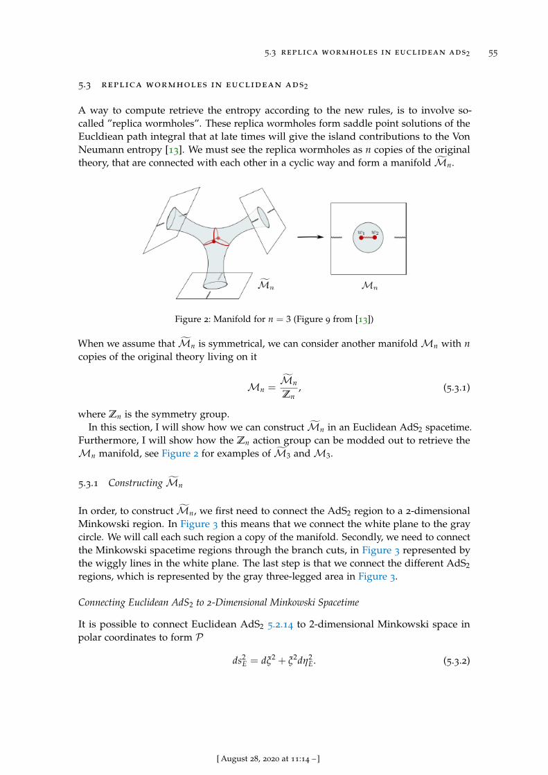
5.3 replica wormholes in euclidean ads2 55
5.3 replica wormholes in euclidean ads2
A way to compute retrieve the entropy according to the new rules, is to involve so-called ”replica wormholes”. These replica wormholes form saddle point solutions of theEucldiean path integral that at late times will give the island contributions to the VonNeumann entropy [13]. We must see the replica wormholes as n copies of the originaltheory, that are connected with each other in a cyclic way and form a manifold Mn.
Figure 2: Manifold for n = 3 (Figure 9 from [13])
When we assume that Mn is symmetrical, we can consider another manifoldMn with ncopies of the original theory living on it
Mn =Mn
Zn, (5.3.1)
where Zn is the symmetry group.In this section, I will show how we can construct Mn in an Euclidean AdS2 spacetime.
Furthermore, I will show how the Zn action group can be modded out to retrieve theMn manifold, see Figure 2 for examples of M3 andM3.
5.3.1 Constructing Mn
In order, to construct Mn, we first need to connect the AdS2 region to a 2-dimensionalMinkowski region. In Figure 3 this means that we connect the white plane to the graycircle. We will call each such region a copy of the manifold. Secondly, we need to connectthe Minkowski spacetime regions through the branch cuts, in Figure 3 represented bythe wiggly lines in the white plane. The last step is that we connect the different AdS2
regions, which is represented by the gray three-legged area in Figure 3.
Connecting Euclidean AdS2 to 2-Dimensional Minkowski Spacetime
It is possible to connect Euclidean AdS2 5.2.14 to 2-dimensional Minkowski space inpolar coordinates to form P
ds2E = dξ2 + ξ2dη2
E. (5.3.2)
[ August 28, 2020 at 11:14 –]
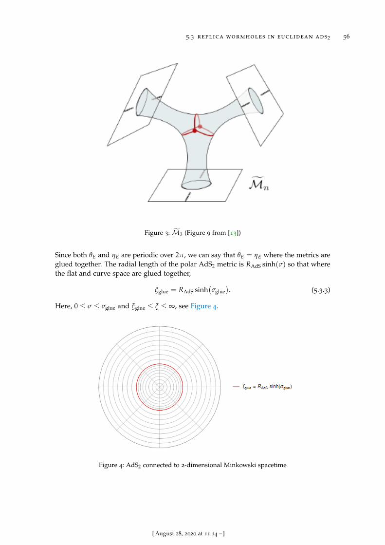
5.3 replica wormholes in euclidean ads2 56
Figure 3: M3 (Figure 9 from [13])
Since both θE and ηE are periodic over 2π, we can say that θE = ηE where the metrics areglued together. The radial length of the polar AdS2 metric is RAdS sinh(σ) so that wherethe flat and curve space are glued together,
ξglue = RAdS sinh(σglue
). (5.3.3)
Here, 0 ≤ σ ≤ σglue and ξglue ≤ ξ ≤ ∞, see Figure 4.
Figure 4: AdS2 connected to 2-dimensional Minkowski spacetime
[ August 28, 2020 at 11:14 –]
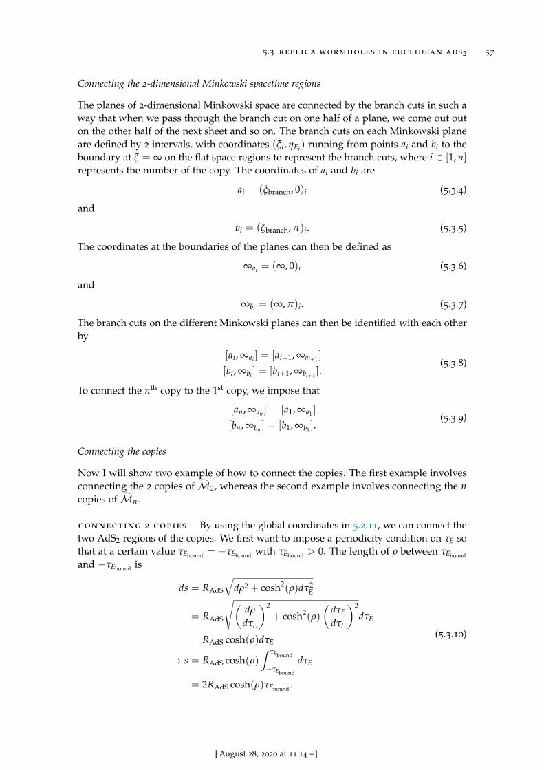
5.3 replica wormholes in euclidean ads2 57
Connecting the 2-dimensional Minkowski spacetime regions
The planes of 2-dimensional Minkowski space are connected by the branch cuts in such away that when we pass through the branch cut on one half of a plane, we come out outon the other half of the next sheet and so on. The branch cuts on each Minkowski planeare defined by 2 intervals, with coordinates (ξi, ηEi ) running from points ai and bi to theboundary at ξ = ∞ on the flat space regions to represent the branch cuts, where i ∈ [1, n]
represents the number of the copy. The coordinates of ai and bi are
ai = (ξbranch, 0)i (5.3.4)
and
bi = (ξbranch, π)i. (5.3.5)
The coordinates at the boundaries of the planes can then be defined as
∞ai = (∞, 0)i (5.3.6)
and
∞bi = (∞, π)i. (5.3.7)
The branch cuts on the different Minkowski planes can then be identified with each otherby
[ai, ∞ai ] = [ai+1, ∞ai+1 ]
[bi, ∞bi ] = [bi+1, ∞bi+1 ].(5.3.8)
To connect the nth copy to the 1st copy, we impose that
[an, ∞an ] = [a1, ∞a1 ]
[bn, ∞bn ] = [b1, ∞b1 ].(5.3.9)
Connecting the copies
Now I will show two example of how to connect the copies. The first example involvesconnecting the 2 copies of M2, whereas the second example involves connecting the ncopies of Mn.
connecting 2 copies By using the global coordinates in 5.2.11, we can connect thetwo AdS2 regions of the copies. We first want to impose a periodicity condition on τE sothat at a certain value τEbound = −τEbound with τEbound > 0. The length of ρ between τEbound
and −τEbound is
ds = RAdS
√dρ2 + cosh2(ρ)dτ2
E
= RAdS
√(dρ
dτE
)2
+ cosh2(ρ)
(dτE
dτE
)2
dτE
= RAdS cosh(ρ)dτE
→ s = RAdS cosh(ρ)∫ τEbound
−τEbound
dτE
= 2RAdS cosh(ρ)τEbound .
(5.3.10)
[ August 28, 2020 at 11:14 –]
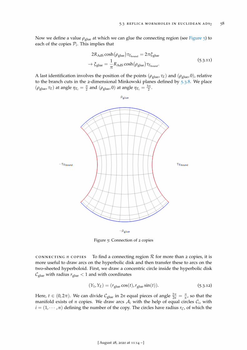
5.3 replica wormholes in euclidean ads2 58
Now we define a value ρglue at which we can glue the connecting region (see Figure 5) toeach of the copies Pi. This implies that
2RAdS cosh(ρglue
)τEbound = 2πξglue
→ ξglue =1π
RAdS cosh(ρglue
)τEbound .
(5.3.11)
A last identification involves the position of the points (ρglue, τE) and (ρglue, 0), relativeto the branch cuts in the 2-dimensional Minkowski planes defined by 5.3.8. We place(ρglue, τE) at angle ηEi = π
2 and (ρglue, 0) at angle ηEi = 3π2 .
Figure 5: Connection of 2 copies
connecting n copies To find a connecting region R for more than 2 copies, it ismore useful to draw arcs on the hyperbolic disk and then transfer these to arcs on thetwo-sheeted hyperboloid. First, we draw a concentric circle inside the hyperbolic diskCglue with radius rglue < 1 and with coordinates
(Y1, YE) = (rglue cos(t), rglue sin(t)). (5.3.12)
Here, t ∈ (0, 2π). We can divide Cglue in 2n equal pieces of angle 2π2n = π
n , so that themanifold exists of n copies. We draw arcs Ai with the help of equal circles Ci, withi = (1, · · · , n) defining the number of the copy. The circles have radius rC , of which the
[ August 28, 2020 at 11:14 –]
5.3 replica wormholes in euclidean ads2 59
centre has distance R to the centre of the hyperbolic disk. The endpoints of Ai should beconnected to Cglue at angles ti1 and ti2 . We can identify the half-angle of the arc
dt =12
(ti2 − ti1) =12
π
n=
π
2n, (5.3.13)
so that
ti2 − ti1 =π
n. (5.3.14)
Furthermore, the angle at the centre of each arc is defined by
∆ti =12
(ti1 + ti2) . (5.3.15)
The boundaries Bi are placed between angles ti2 and t(i+1)1, with coordinates
(Y1Bi, YEBi
) = (rglue cos(ti), rglue sin(ti)) for ti ∈[ti2 , t(i+1)1
](5.3.16)
The centres of the circles Ci are located at
(Y1, YE) = (R cos(∆ti), R sin(∆ti)) . (5.3.17)
Trigonometry shows that the radius of Ci is
rC = rglue tan(dt). (5.3.18)
The distance between the middle points of Cglue and Ci is
R =√
r2glue + r2
glue tan2(dt)
= rglue sec(dt).(5.3.19)
The distance between the point (0, 0) and (r∆, ∆ti) is
r∆ = R− rC= rglue sec(dt)− rglue tan(dt)
= rglue(sec(dt)− tan(dt)).
(5.3.20)
The coordinates of Ci can be defined as(
Y1Ci, YECi
)= (ri cos(ti), ri sin(ti)). Since we
already now the coordinates of the centres of Ci in 5.3.17, we now want to solve thefollowing equation for ri
r2C = (ri cos(ti)− R cos(∆ti))
2 + (ri sin(ti)− R sin(∆ti))2
→ r2glue tan2(dt) =
(ri cos(ti)− rglue sec(dt) cos(∆ti)
)2+(ri sin(ti)− rglue sec(dt) sin(∆ti)
)2
→ ri = rglue sec(dt)
(cos(ti − ∆ti)±
√12
(cos(2(ti − ∆ti))− cos(2dt))
)
= rglue sec(dt)(
cos(ti − ∆ti)±√− sin(ti − ∆ti − dt) sin(ti − ∆ti + dt)
),
(5.3.21)
[ August 28, 2020 at 11:14 –]

5.3 replica wormholes in euclidean ads2 60
to find the coordinates of Ci. The coordinates of Ci are then
(Y1Ci
, YECi
)= rglue sec(dt)
(cos(ti − ∆ti)±
√− sin(ti − ∆ti − dt) sin(ti − ∆ti + dt)
)× (cos(ti), sin(ti)). (5.3.22)
For the arcs Ai, we need the area of Ci for ri < 1, which is given by the solution of ri withthe minus sign. The coordinates of the arcs Ai then are
(Y1Ai
, YEAi
)= rglue sec(dt)
(cos(ti − ∆ti)−
√− sin(ti − ∆ti − dt) sin(ti − ∆ti + dt)
)× (cos(ti), sin(ti)) for ti ∈ [ti1 , ti2 ]. (5.3.23)
In Figure 6, we show an example of R for n = 3 with the locations of ti1 , ti2 and ∆ti. Thedashed lines represent the separation of the different copies. As we can see in the figure,each copy i is bounded by the following interval
(Y1i , YEi ) = (r cos(t), r sin(t))
for t ∈ [∆ti, ti2 ] and r ∈ [0, ri]
for t ∈ [ti2 , t(i+1)1] and r ∈ [0, rglue]
for t ∈ [t(i+1)1, ∆t(i+1)] and r ∈ [0, r(i+1)].
(5.3.24)
Figure 6: Example of R for n = 3
[ August 28, 2020 at 11:14 –]
5.3 replica wormholes in euclidean ads2 61
We can now transform the coordinates on the hyperbolic disk to coordinates on thehyperboloid, by using 5.2.9. The coordinates on the hyperbolic disk are
(Y1, YE) = (r cos(t), r sin(t)) (5.3.25)
with metric
ds2 = dr2 + r2dt2 (5.3.26)
for t periodic over 2π and r ∈ [0, 1). The transformation then implies that the coordinateson the hyperboloid are
(X0, X1, XE) =RAdS
1− r2
(1 + r2, 2r cos(t), 2r sin(t)
)(5.3.27)
with metric
ds2 = 4R2AdS
dr2 + r2dt2
(r2 − 1)2 . (5.3.28)
On the hyperboloid, each copy i is now bounded by
(X0i , X1i , XEi ) =RAdS
1− r2
(1 + r2, 2r cos(t), 2r sin(t)
)
for t ∈ [∆ti, ti2 ] and r ∈ [0, ri]
for t ∈ [ti2 , t(i+1)1] and r ∈ [0, rglue]
for t ∈ [t(i+1)1, ∆t(i+1)] and r ∈ [0, r(i+1)].
(5.3.29)
In order for the manifold to be smooth, we need two copies of R and call them RA andRB. Now we want to rename the points ti1 and ti2 , so that each copy of the manifold nowhas arc endpoints ia and ib on both RA and RB so that
iaA = ti2Aand ibA = t(i+1)1A
,
iaB = ti2Band ibB = t(i+1)1B
.(5.3.30)
We can now connect RA and RB so that the boundary of each copy is represented by asemicircle on RA and a semicircle on RB. In terms of the arc endpoints, this means
iaA = iaB = ia and ibA = ibB = ib. (5.3.31)
Each boundary line Bi on RA now represents a semicircle with angle 0 to π and eachboundary line Bi on RB now represents a semicircle with angle π to 2π, see Figure 7 forthe example of n = 3.
The circumference of each circle that is formed by the connection of these semicircles Sishould then be the circumference of the gluing circle on Pi, 2πξglue. The length of Bi isrglue
πn , so that the circumference of Si also is rglue
2πn , which means
2πξglue = rglue2π
n
→ ξglue =rglue
n.
(5.3.32)
A last identification involves the position of the points ia and ib, relative to the branch cutsin the 2-dimensional Minkowski planes defined by 5.3.8. We place ia at angle ηEi = π
2and ib at angle ηEi = 3π
2 .
[ August 28, 2020 at 11:14 –]

5.3 replica wormholes in euclidean ads2 62
Figure 7: Example of RA and RB for n = 3
5.3.2 IdentifyingMn
As we saw in the example of M3, the manifold Mn is rotational symmetric around thepoints (0, 0) on both RA and RB. When we mod out the Zn action group, these pointsbecome so-called ”fixed points” with a conical deficit angle of 2π
n . We call these pointswA and wB (see Figure 8 for an example of M3).
Figure 8: Example of RA and RB for n = 3 with the fixed points wA and wB
The Zn action group is formed by identifying different regions on Mn with each other.The most trivial identification is, is the identification of the regions Pi of each copy, with
[ August 28, 2020 at 11:14 –]
5.4 replica trick on the replica manifold 63
each other. For the regions RA and RB, the identification of the different copies witheach other means that we should relate the coordinates (r(t), t) of one copy to the samecoordinates on another copy
(r(t), t) =
(r(
t +2π(i− 1)
n
), t +
2π(i− 1)
n
), (5.3.33)
with i ∈ (1, n). After modding out the Zn action group, the region between the pointswA and wB forms a new branch cut of length 2r∆ = 2rglue(sec
(π2n
)− tan
(π2n
)).
5.4 replica trick on the replica manifold
In this section, we will provide an example of how to perform the replica trick on thereplica manifold Mn. We can start by computing the partition function Zn on Mn
Zn = Z[Mn]. (5.4.1)
Then the entropy can be computed by performing the replica trick 2.3.18. The partitionfunction for the whole system is a sum of the gravitational action IE,grav and the logarithmof the partition function for the quantum fields on the geometry as we saw in 5.1.19
ln Zn = −IE,grav + ln Zmat[Mn]. (5.4.2)
This is an effective action for the geometry, so that the integral over the geometriesmust be evaluated as a saddle point. The branch cuts on the 2-dimensional Minkowskispacetime represent the region R for the radiation in 5.1.21. We can place twist operatorsTn at the end points of these branch cuts to connect the different copies with each other.These twist operators obey the conditions that are given by 5.3.9 (see [59]). Wen we modout the Zn action group, we can also place twist operators at the fixed points of the Zn
action group wA and wB, with conical deficit angle 2πn . Now we can translate 5.4.2, to an
equation that involves the new manifoldMn. We can place codimension-two ”cosmicbranes” on the positions of the fixed points at wA and wB, with tension
Tn =n− 14nGN
. (5.4.3)
Because of their codimension-two, these cosmic branes represent just points in a 2-dimensional geometry, but become ”cosmic strings” 4-dimensional spacetime. We canthen replace the gravitational action in 5.4.2 by
Igrav[Mn] = n(
Igrav[Mn] + Tn
∫Σd−2
√g)
= nIgrav[Mn] +n− 14GN
∫Σd−2
√g, (5.4.4)
where we added the action of the cosmic branes. When n = 1, the manifold M1 =M1
which is a solution of the total action Itot1 . To find the manifoldMn for n ∼ 1 we need to
add the action of the cosmic branes
limn→1
Itot = nI1 + δI. (5.4.5)
Here, δI arises from the effect of the tension Tn of the cosmic branes and of the effect ofthe insertion of the twist operators at these cosmic branes. When n ∼ 1, the contribution
[ August 28, 2020 at 11:14 –]

5.4 replica trick on the replica manifold 64
of these effects is of order n− 1. When we perturb the action from the solutionM1, wecan see that δI drops out of the geometry, since the effects are of order n− 1. The term δIis then proportional to the generalised entropy at the positions of the cosmic branes wi
−δ
(ln Z
n
)= δ
(In
)= (n− 1)Sgen(wi) (5.4.6)
which now represent the QES X as described in the previous section. The region betweenwA and wB can then be seen as the island region I in 5.1.21 when we extremise 5.4.6.
[ August 28, 2020 at 11:14 –]
6C O N C L U S I O N S & F U T U R E R E S E A R C H
6.1 conclusions
In this thesis, I examined a wide range of topics. All of these topics can be seen in thelight of the Von Neumann entropy. The first topic I examined was how the Von Neumannentropy can be retrieved in statistical quantum mechanics with the help of the densitymatrix and the partition function. An important ensemble in quantum mechanics is thecanonical ensemble, which represents the possible states of a system that is in a thermalequilibrium with a heat bath. The partition function in the canonical ensemble can beused to retrieve the values for the energy, the free energy and the entropy of a system.
A useful method to calculate the entropy of a system is the replica trick. The replicatrick uses Renyi entropies in the limit n → 1. To use the replica trick we only need tocompute the value of the partition function, which in most cases is easier to achieve thento compute the density matrix. We can perform the replica trick when we assume thatwe have n copies of the partition function.
Wick rotating the time dimension hands us a magical method to determine the ther-modynamic properties of quantum systems. By performing the Euclidean path integrals,we can compute the partition function, which gives us the opportunity to perform thereplica trick. A good example of how the Euclidean time direction represents tempera-ture, is given by the Unruh effect. Here, a uniformly accelerated observer experience atemperature that is proportional to the periodicity of the Euclidean time.
The entropy of 2-dimensional conformal field theories is determined by the Cardyformula. I recovered the Cardy formula from the computation of the entropy of amassless free scalar field in 2-dimensional Minkowski spacetime.
A common way to compute path integrals is by using a saddle point approximation. Inthis approximation, the action is varied around the classical action of the path integral inorder to retrieve its highest contribution. In black hole thermodynamics, a saddle pointapproximation is required to compute the Einstein-Hilbert action. Otherwise, the pathintegral diverges.
To compute the right entropy for black holes and the Hawking radiation, we canintroduce replica wormhole solutions to the path integral. These replica wormholes forma manifold that consists of n copies of the original black hole. In this thesis we foundthe metric for such a manifold in AdS2. Eventually, we can calculate Zn and perform thereplica trick over this manifold to reproduce the right entropy of the Hawking radiation.
65
[ August 28, 2020 at 11:14 –]
6.2 future research 66
6.2 future research
The research that was executed in this thesis can in many ways be extended to future re-search. The path integrals that were performed in this thesis gave exact results. However,for most path integrals in quantum field theories, the results must be approximated. TheEuclidean path integrals in black hole thermodynamics can even only be approximated.An idea is to compute gravitational path integrals on a physical gravitational background,to see if the thermality of the results is in line with thermality that you would expectfrom regular black hole thermodynamics.
Another extension involves the replica wormholes. Here, I constructed the n-manifoldin AdS2, but it would be interesting to see how this construction works in higherdimensions. It could also be possible to extend this field of research to curved spacetimesother than AdS to get a better grip of the meaning of the replica wormholes in thephysical universe.
Something that is not well understood is how the replica wormholes should be inter-preted physically. Are these connections that really exist when a black hole evaporates,or do they just function as a mathematical construction to serve the purpose of a rightanswer.
Furthermore, research must be done to understand the new rules in non-AdS space-times. The rules have been derived from results that are closely related to string theory,but need to be tested on more physical spacetimes, to see if the Black Hole InformationParadox can really be solved.
[ August 28, 2020 at 11:14 –]
AA P P E N D I C E S
a.1 replica trick
The replica trick can be derived in terms of the denisty matrix ρ
limn→1Sn = limn→1
ln Tr ρn
1− n
= limn→1
∂n(ln Tr ρn)
∂n(1− n)
= − limn→1
∂n(Tr ρn)
Tr ρn
= − limn→1
∂n(Tr ρn)
= − limn→1
∂n(Tr en ln ρ)
= − limn→1
Tr ρn ln ρ
= −Tr ρ ln ρ
= S
(A.1.1)
and in terms of its eigen values pi
limn→1
Sn = limn→1
ln ∑∞i=0 pn
i1− n
= limn→1
∂n(ln ∑∞i=0 pn
i )
∂n(1− n)
= − limn→1
∑∞i=0 ∂n(pn
i )
∑∞i=0 pn
i
= − limn→1
∞
∑i=0
∂n(pni )
= − limn→1
∞
∑i=0
∂n(en ln pi )
= − limn→1
∞
∑i=0
pni ln pi
= −∞
∑i=0
pi ln pi
= S.
(A.1.2)
67
[ August 28, 2020 at 11:14 –]
A.2 saddle point approximation 68
a.2 saddle point approximation
Here, I will show the derivation of the saddle point approximation in quantum mechanicsand in quantum field theory.
a.2.1 Quantum Mechanics
If we recall that the propagator for the Euclidean action is
K(xi, x f , τ) =⟨
x f , τf∣∣ e−(τf−τi)H |xi, τi〉 = N
∫ x(τf )=x f
x(τi)=xi
D[x]e−IE[x(τ)]. (A.2.1)
We can vary the Euclidean action
IE[x(τ)] =∫ τf
τi
L (x(τ), x(τ)) dτ (A.2.2)
so that
δIE[x(τ)] = 0 (A.2.3)
due to the Euler-Lagrange equations of motion. Since the path integral is dominated bypaths close to the classical action, we can define
x(τ) = xcl(τ) + δx(τ), (A.2.4)
where δx(τ) counts for the deviations of x of the classical path, so that δx(τi) = δx(τf ) =
0. Here τi and τf stand for the initial and final points of the path respectively. Furthermore,xcl(τi) = xi and xcl(τf ) = x f . If we expand the action around xcl(τ), it becomes
IE[x(τ)] = IE[xcl] +∫ τf
τi
dτ1δIE[x]
δx(τ1)
∣∣∣∣x=xcl
δx(τ1)
+12
∫ τf
τi
dτ1
∫ τf
τi
dτ2δ2 IE[x]
δx(τ1)δx(τ2)
∣∣∣∣x=xcl
δx(τ1)δx(τ2) +O(δx3). (A.2.5)
In terms of the Lagrangian this is∫ τf
τi
dτ1δIE[x]
δx(τ1)
∣∣∣∣x=xcl
δx(τ1) =∫ τf
τi
dτ1δ
δx(τ1)
(∫ τf
τi
L (x(τ), x(τ)) dτ
)∣∣∣∣x=xcl
δx(τ1).
(A.2.6)
[ August 28, 2020 at 11:14 –]
A.2 saddle point approximation 69
Now
δ
δx(τ)
(∫ τf
τi
L(x(τ′), x(τ′)
)dτ′)∣∣∣∣
x=xcl
δx(τ)
=∫ τf
τi
dτ′(
∂L(x, x)
∂x(τ′)
∣∣∣∣x=xcl
δx(τ′)
δx(τ)+
∂L(x, x)
∂x(τ′)
∣∣∣∣x=xcl
δx(τ′)
δx(τ)
)δx(τ)
=∫ τf
τi
dτ′(
∂L(x, x)
∂x(τ′)
∣∣∣∣x=xcl
δx(τ′)
δx(τ)+
∂L(x, x)
∂x(τ′)
∣∣∣∣x=xcl
ddτ′
δx(τ′)
δx(τ)
)δx(τ)
=∫ τf
τi
dτ′(
∂L(x, x)
∂x(τ′)
∣∣∣∣x=xcl
δ(τ′ − τ) +∂L(x, x)
∂x(τ′)
∣∣∣∣x=xcl
ddτ′
δ(τ′ − τ)
)δx(τ)
=
(∂L(x, x)
∂x(τ)
∣∣∣∣x=xcl
+∂L(x, x)
∂x(τ)
∣∣∣∣x=xcl
ddτ
)δx(τ)
=∂L(x, x)
∂x(τ)
∣∣∣∣x=xcl
δx(τ) +∂L(x, x)
∂x(τ)
∣∣∣∣x=xcl
δx(τ),
(A.2.7)
so that ∫ τf
τi
dτ1δIE[x]
δx(τ1)
∣∣∣∣x=xcl
δx(τ1)
=∫ τf
τi
dτ
(∂L(x, x)
∂x(τ)
∣∣∣∣x=xcl
δx(τ) +∂L(x, x)
∂x(τ)
∣∣∣∣x=xcl
δx(τ)
).
(A.2.8)
If we use the chain rule and the fact that δx(τi) = δx(τf ) = 0∫ τf
τi
dτ1δIE[x]
δx(τ1)
∣∣∣∣x=xcl
δx(τ1)
=∫ τf
τi
dτ
(∂L(x, x)
∂x(τ)
∣∣∣∣x=xcl
− ddτ
∂L(x, x)
∂x(τ)
∣∣∣∣x=xcl
)δx(τ) +
(∂L(x, x)
∂x(τ)
∣∣∣∣x=xcl
δx(τ)
)∣∣∣∣∣τf
τi
=∫ τf
τi
dτ
(∂L(x, x)
∂x(τ)
∣∣∣∣x=xcl
− ddτ
∂L(x, x)
∂x(τ)
∣∣∣∣x=xcl
)δx(τ).
(A.2.9)
If we minimize the action, we can recognise the Euler-Lagrange equation of motion∫ τf
τi
dτ1δIE[x]
δx(τ1)
∣∣∣∣x=xcl
δx(τ1) = 0
→ ∂L(x, x)
∂x(τ)
∣∣∣∣x=xcl
− ddτ
∂L(x, x)
∂x(τ)
∣∣∣∣x=xcl
= 0.(A.2.10)
The second variation of the action is∫ τf
τi
dτ1
∫ τf
τi
dτ2δ2 IE[x]
δx(τ1)δx(τ2)
∣∣∣∣x=xcl
δx(τ1)δx(τ2)
=∫ τf
τi
dτ1
∫ τf
τi
dτ2δ2
δx(τ1)δx(τ2)
(∫ τf
τi
L (x(τ), x(τ)) dτ
)∣∣∣∣x=xcl
δx(τ1)δx(τ2).
(A.2.11)
[ August 28, 2020 at 11:14 –]
A.2 saddle point approximation 70
If we recall that
δ
δx(τ)
(∫ τf
τi
L(x(τ′), x(τ′)
)dτ′)∣∣∣∣
x=xcl
δx(τ)
=∂L(x, x)
∂x(τ)
∣∣∣∣x=xcl
δx(τ) +∂L(x, x)
∂x(τ)
∣∣∣∣x=xcl
δx(τ),(A.2.12)
this becomes∫ τf
τi
dτ1
∫ τf
τi
dτ2δ2 IE[x]
δx(τ1)δx(τ2)
∣∣∣∣x=xcl
δx(τ1)δx(τ2)
=∫ τf
τi
dτ1δ
δx(τ1)
∫ τf
τi
dτ
(∂L(x, x)
∂x(τ)
∣∣∣∣x=xcl
δx(τ) +∂L(x, x)
∂x(τ)
∣∣∣∣x=xcl
δx(τ)
)δx(τ1).
(A.2.13)
Now
δ
δx(τ1)
∫ τf
τi
dτ
(∂L(x, x)
∂x(τ)
∣∣∣∣x=xcl
δx(τ) +∂L(x, x)
∂x(τ)
∣∣∣∣x=xcl
δx(τ)
)δx(τ1)
=δ
δx(τ1)
∫ τf
τi
dτ∂L(x, x)
∂x(τ)
∣∣∣∣x=xcl
δx(τ)δx(τ1) +δ
δx(τ1)
∫ τf
τi
dτ∂L(x, x)
∂x(τ)
∣∣∣∣x=xcl
δx(τ)δx(τ1),
(A.2.14)
where
δ
δx(τ1)
∫ τf
τi
dτ∂L(x, x)
∂x(τ)
∣∣∣∣x=xcl
δx(τ)δx(τ1)
=∫ τf
τi
dτ
(∂2L(x, x)
∂x(τ)2
∣∣∣∣x=xcl
δx(τ)
δx(τ1)+
∂2L(x, x)
∂x(τ)∂x(τ)
∣∣∣∣x=xcl
δx(τ)
δx(τ1)
)δx(τ1)δx(τ)
=∫ τf
τi
dτ
(∂2L(x, x)
∂x(τ)2
∣∣∣∣x=xcl
δx(τ)
δx(τ1)+
∂2L(x, x)
∂x(τ)∂x(τ)
∣∣∣∣x=xcl
ddτ
δx(τ)
δx(τ1)
)δx(τ1)δx(τ)
=∫ τf
τi
dτ
(∂2L(x, x)
∂x(τ)2
∣∣∣∣x=xcl
δ(τ − τ1) +∂2L(x, x)
∂x(τ)∂x(τ)
∣∣∣∣x=xcl
ddτ
δ(τ − τ1)
)δx(τ1)δx(τ)
=
(∂2L(x, x)
∂x(τ)2
∣∣∣∣x=xcl
δx(τ) +∂2L(x, x)
∂x(τ)∂x(τ)
∣∣∣∣x=xcl
ddτ
δx(τ)
)δx(τ)
=∂2L(x, x)
∂x(τ)2
∣∣∣∣x=xcl
δx(τ)2 +∂2L(x, x)
∂x(τ)∂x(τ)
∣∣∣∣x=xcl
δx(τ)δx(τ)
(A.2.15)
[ August 28, 2020 at 11:14 –]
A.2 saddle point approximation 71
and
δ
δx(τ1)
∫ τf
τi
dτ∂L(x, x)
∂x(τ)
∣∣∣∣x=xcl
δx(τ)δx(τ1)
=∫ τf
τi
dτ
(∂2L(x, x)
∂x(τ)∂x(τ)
∣∣∣∣x=xcl
δx(τ)
δx(τ1)+
∂L(x, x)
∂x(τ)
∣∣∣∣x=xcl
δx(τ)
δx(τ1)
)δx(τ1)δx(τ)
=∫ τf
τi
dτ
(∂2L(x, x)
∂x(τ)∂x(τ)
∣∣∣∣x=xcl
δx(τ)
δx(τ1)+
∂L(x, x)
∂x(τ)
∣∣∣∣x=xcl
ddτ
δx(τ)
δx(τ1)
)δx(τ1)δx(τ)
=∫ τf
τi
dτ
(∂2L(x, x)
∂x(τ)∂x(τ)
∣∣∣∣x=xcl
δ(τ − τ1) +∂L(x, x)
∂x(τ)
∣∣∣∣x=xcl
ddτ
δ(τ − τ1)
)δx(τ1)δx(τ)
=
(∂2L(x, x)
∂x(τ)∂x(τ)
∣∣∣∣x=xcl
δx(τ) +∂L(x, x)
∂x(τ)
∣∣∣∣x=xcl
ddτ
δx(τ)
)δx(τ)
=∂2L(x, x)
∂x(τ)∂x(τ)
∣∣∣∣x=xcl
δx(τ)δx(τ) +∂L(x, x)
∂x(τ)
∣∣∣∣x=xcl
δx(τ)2,
(A.2.16)
so that∫ τf
τi
dτ1
∫ τf
τi
dτ2δ2 IE[x]
δx(τ1)δx(τ2)
∣∣∣∣x=xcl
δx(τ1)δx(τ2)
=∫ τf
τi
dτ
(∂2L(x, x)
∂x(τ)2
∣∣∣∣x=xcl
δx(τ)2 +∂2L(x, x)
∂x(τ)∂x(τ)
∣∣∣∣x=xcl
δx(τ)δx(τ)
+∂2L(x, x)
∂x(τ)∂x(τ)
∣∣∣∣x=xcl
δx(τ)δx(τ) +∂L(x, x)
∂x(τ)
∣∣∣∣x=xcl
δx(τ)2
)
=∫ τf
τi
dτ
(∂2L(x, x)
∂x(τ)2
∣∣∣∣x=xcl
δx(τ)2 + 2∂2L(x, x)
∂x(τ)∂x(τ)
∣∣∣∣x=xcl
δx(τ)δx(τ)
+∂L(x, x)
∂x(τ)
∣∣∣∣x=xcl
δx(τ)2
).
(A.2.17)
The whole variation of the action becomes
IE[x(τ)]
= IE[xcl] +∫ τf
τi
dτ1δIE[x]
δx(τ1)
∣∣∣∣x=xcl
δx(τ1)
+12
∫ τf
τi
dτ1
∫ τf
τi
dτ2δ2 IE[x]
δx(τ1)δx(τ2)
∣∣∣∣x=xcl
δx(τ1)δx(τ2) +O(δx3)
=∫ τf
τi
L (x(τ), x(τ))|x=xcldτ +
12
∫ τf
τi
dτ
(∂2L(x, x)
∂x(τ)2
∣∣∣∣x=xcl
δx(τ)2
+ 2∂2L(x, x)
∂x(τ)∂x(τ)
∣∣∣∣x=xcl
δx(τ)δx(τ) +∂L(x, x)
∂x(τ)
∣∣∣∣x=xcl
δx(τ)2
)+O(δx3),
(A.2.18)
or just
IE[x(τ)] = IE[xcl] + IE[δx]. (A.2.19)
[ August 28, 2020 at 11:14 –]
A.2 saddle point approximation 72
Because of the variation of x(τ), the propagator becomes
K(x f , τf ; xi, τi) = N∫ x(τf )=x f
x(τi)=xi
D[x]e−IE[x(τ)]
= N∫ x(τf )=x f
x(τi)=xi
D[x]e−(IE[xcl]+IE[δx])
= N e−IE[xcl]∫ δx(τf )=0
δx(τi)=0D[δx]e−IE[δx],
(A.2.20)
since D[x] only depends on δx.
Different Method of Variation of the Action
Remarkably, we would see the same result if we immediately plug in the expansionaround x(τ)
x(τ) = xcl(τ) + δx(τ). (A.2.21)
The then action becomesIE[x(τ)]
=m2
∫ τf
τi
(x(τ)2 + ω2x(τ)2) dτ
=m2
∫ τf
τi
((xcl(τ) + δx(τ))2 + ω2 (xcl(τ) + δx(τ))2
)dτ
=m2
∫ τf
τi
(xcl(τ)2 + 2xcl(τ)δx(τ) + δx(τ)2 + ω2 (xcl(τ)2 + 2xcl(τ)δx(τ) + δx(τ)2)) dτ
=m2
∫ τf
τi
(xcl(τ)2 + ω2xcl(τ)2) dτ + m
∫ τf
τi
(xcl(τ)δx(τ) + ω2xcl(τ)δx(τ)
)dτ
+m2
∫ τf
τi
(δx(τ)2 + ω2δx(τ)2) dτ
= IE[xcl] + IE[δx] + m∫ τf
τi
(xcl(τ)δx(τ) + ω2xcl(τ)δx(τ)
)dτ.
(A.2.22)
After integration by parts and following the boundary conditions that δx(τi) = δx(τf ) = 0
m∫ τf
τi
(xcl(τ)δx(τ)) dτ
= m xcl(τ)δx(τ)|τfτi −m
∫ τf
τi
(xcl(τ)δx(τ)) dτ
= −m∫ τf
τi
(xcl(τ)δx(τ)) dτ.
(A.2.23)
Using the Euler-Lagrange equation of motion, the third term becomes
m∫ τf
τi
(xcl(τ)δx(τ) + ω2xcl(τ)δx(τ)
)dτ
= −m∫ τf
τi
(xcl(τ)δx(τ)−ω2xcl(τ)δx(τ)
)dτ
= 0,
(A.2.24)
so that again we have the same term for the action
IE[x(τ)] = IE[xcl] + IE[δx]. (A.2.25)
[ August 28, 2020 at 11:14 –]
A.2 saddle point approximation 73
a.2.2 Free Scalar Field Theory
Just like we did for the quantum mechanical path integral, it is possible to expand thefield around a classical field φ = φcl + δφ(x) where δφ(x) reflects the fluctuations of thefield. We imply that these fluctuations do not occur at the boundary of the space-time, sothat δφ(τi,~x) = δφ(τf ,~x) = 0 and δφ(τ,−∞) = δφ(τ, ∞) = 0
I[φ(x)] = I[φcl(x)] +∫
ddx′δI[φ(x)]
δφ(x′)
∣∣∣∣φ=φcl
δφ(x′)
+12
∫ddx′
∫ddx′′
δ2 I[φ(x)]
δφ(x′)δφ(x′′)
∣∣∣∣φ=φcl
δφ(x′)δφ(x′′) +O(δφ3), (A.2.26)
where due to principle of least action
δI[φ(x)] = 0. (A.2.27)
In terms of the Lagrangian density
L[φ(x),∇µφ(x), gµν(x)
]=√|g(x)|L0
[φ(x),∇µφ(x), gµν(x)
]=√|g(x)|L0
[φ(x), ∂µφ(x), gµν(x)
],
(A.2.28)
we can write
δI[φ(x)] =∫
ddx′δI[φ(x)]
δφ(x′)
∣∣∣∣φ=φcl
δφ(x′)
=∫
ddx
∂L[φ,∇αφ, gαβ
]∂φ(x)
∣∣∣∣∣φ=φcl
δφ(x) +∂L[φ,∇αφ, gαβ
]∂(∂µφ(x))
∣∣∣∣∣φ=φcl
δ(∂µφ(x))
=∫
ddx
∂√|g(x)|L0
[φ, ∂αφ, gαβ
]∂φ(x)
∣∣∣∣∣φ=φcl
δφ(x)
+∂√|g(x)|L0
[φ, ∂αφ, gαβ
]∂(∂µφ(x))
∣∣∣∣∣φ=φcl
δ(∂µφ(x))
.
(A.2.29)
Here, due to partial integration
∂√|g(x)|L0
[φ, ∂αφ, gαβ
]∂(∂µφ(x))
∣∣∣∣∣φ=φcl
∂µ(δφ(x)) = ∂µ
∂√|g(x)|L0
[φ, ∂αφ, gαβ
]∂(∂µφ(x))
∣∣∣∣∣φ=φcl
δφ(x)
− ∂µ
∂√|g(x)|L0
[φ, ∂αφ, gαβ
]∂(∂µφ(x))
∣∣∣∣∣φ=φcl
δφ(x)
.
(A.2.30)
[ August 28, 2020 at 11:14 –]
A.2 saddle point approximation 74
Due to the divergence theorem, the term with the total derivative can be written as ad− 1-integral over the boundary of the space-time
∫Ω
ddx∂µ
∂√|g(x)|L0
[φ, ∂αφ, gαβ
]∂(∂µφ(x))
∣∣∣∣∣φ=φcl
δφ(x)
=∫
∂Ωdd−1xnµ
∂√|h(x)|L0
[φ, ∂αφ, gαβ
]∂(∂µφ(x))
∣∣∣∣∣φ=φcl
δφ(x)
= 0,
(A.2.31)
because of the boundary conditions. Here, hµν(x) is the metric of the boundary and nµ
the unit normal of the boundary. Now we can write the action as
δI[φ(x)]
=∫
ddx
∂√|g(x)|L0
[φ, ∂αφ, gαβ
]∂φ(x)
∣∣∣∣∣φ=φcl
− ∂µ
∂√|g(x)|L0
[φ, ∂αφ, gαβ
]∂(∂µφ(x))
∣∣∣∣∣φ=φcl
δφ(x)
=∫
ddx
√|g(x)|∂L0
[φ, ∂αφ, gαβ
]∂φ(x)
∣∣∣∣∣φ=φcl
− ∂µ
√|g(x)|∂L0
[φ, ∂αφ, gαβ
]∂(∂µφ(x))
∣∣∣∣∣φ=φcl
δφ(x).
(A.2.32)
The variation of the action then gives the Euler-Lagrange equation
δI[φ(x)] = 0
→∂L0
[φ, ∂αφ, gαβ
]∂φ(x)
∣∣∣∣∣φ=φcl
− 1√|g(x)|
∂µ
√|g(x)|∂L0
[φ, ∂αφ, gαβ
]∂(∂µφ(x))
∣∣∣∣∣φ=φcl
= 0.
(A.2.33)
If we use
L0[φ(x), ∂µφ(x), gµν(x)
]= −1
2gµν(x)∂µφ(x)∂νφ(x)−V [φ(x)] , (A.2.34)
we get
1√|g(x)|
∂µ
(√|g(x)|1
2
(gαβδ
µα ∂βφcl(x) + gαβ∂αφcl(x)δν
β
))−V ′[φcl(x)]
=1√|g(x)|
∂µ
(√|g(x)|1
2
(gµβ∂βφcl(x) + gαν∂αφcl(x)
))−V ′[φcl(x)]
=1√|g(x)|
∂µ
(√|g(x)|gµν∂νφcl(x)
)−V ′[φcl(x)]
= 0.
(A.2.35)
If we now use the identity
∇µVµ =1√|g(x)|
∂µ
(√|g(x)|Vµ
)(A.2.36)
[ August 28, 2020 at 11:14 –]
A.3 direct calculation of the propagator of the free particle 75
and the fact that ∇µφ(x) = ∂µφ(x), we can write the Euler-Lagrange equation as
∇µgµν∇νφcl(x)−V ′[φcl(x)] = gµν∇µ∇νφcl(x)−V ′[φcl(x)]
= 0.(A.2.37)
Likewise, the second variation of the action in terms of the Lagrangian density gives
12
∫ddx′
∫ddx′′
δ2 I[φ(x)]
δφ(x′)δφ(x′′)
∣∣∣∣φ=φcl(x)
δφ(x′)δφ(x′′)
=12
∫ddx√|g(x)|
(−gµν∂µ∂ν −V ′′[φcl(x)]
)δφ(x)2
=12
∫ddx√|g(x)|δφ(x)
(gµν∂µ∂ν −V ′′[φcl(x)]
)δφ(x),
(A.2.38)
due to the boundary conditions. The whole variation of the action then becomes
I[φ(x)] = I[φcl(x)] +12
∫ddx√|g(x)|δφ(x)
(gµν∂µ∂ν −V ′′[φcl(x)]
)δφ(x)
+O(δφ3). (A.2.39)
a.3 direct calculation of the propagator of the free particle
The propagator for the free particle can be directly computed by
K(x f , τf ; xi, τi) =⟨
x f , τf∣∣ e−(τf−τi)H |xi, τi〉
=⟨
x f , τf∣∣ e−(τf−τi)
p22m |xi, τi〉 .
(A.3.1)
By inserting a complete set of eigenstates 1 =∫
dp |p〉 〈p|, we obtain
K(x f , τf ; xi, τi) =∫
dp⟨
x f∣∣p⟩ e−(τf−τi)
p22m 〈p|xi〉 . (A.3.2)
We can then use the identity 〈x|p〉 = eipx√
2π, so that
K(x f , τf ; xi, τi) =∫
dpeipx f
√2π
e−(τf−τi)p22m
e−ipxi
√2π
=1
2π
∫dpe−(τf−τi)
p22m +ip(x f−xi).
(A.3.3)
By using the identity∫
dxe−ax2+bx =√
πa e
b24a , we retrieve
K(x f , τf ; xi, τi) =1
2π
√2mπ
(τf − τi)e−m
2
(x f −xi)2
τf −τi
=
√m
2π(τf − τi)e−m
2
(x f −xi)2
τf −τi .
(A.3.4)
[ August 28, 2020 at 11:14 –]
A.4 direct calculation of the partition function of the harmonic oscillator 76
a.4 direct calculation of the partition function of the harmonic
oscillator
The partition function of the harmonic oscillator can also be derived directly [60]. Theidea is that we start by installing the boundary conditions. In terms of the path integral,the partition function is
Z = N∫ x(β)=x(0)
D[x]e−IE[x(τ)]
= N∫ x(β)=x(0)
D[x] exp−m
2
∫ β
0
(x(τ)2 + ω2x(τ)2) dτ
.
(A.4.1)
Because of the periodic boundary condition x(β) = x(0), x(τ) can be expressed as aFourier series
x(τ) =∞
∑n=−∞
xneiωnτ, (A.4.2)
with
ωn =2πn
β. (A.4.3)
Here, x(τ) ∈ R, such that x∗(τ) = x(τ)→ x∗n = x−n. If xn = an + ibn → x∗n = an − ibn =
x−n = a−n + ib−n → a−n = an & b−n = −bn. Since b0 = 0 this changes to
x(τ) = a0 +∞
∑n=1
[(an + ibn)eiωnτ + (an − ibn)e−iωnτ
], (A.4.4)
so that the Euclidean action becomes
IE[x(τ)] =m2
∫ β
0
(x(τ)2 + ω2x(τ)2)
=m2
∫ β
0
(−∑
n,mωnxneiωnτωmxmeiωmτ + ω2 ∑
n,mxneiωnτxmeiωmτ
)dτ
=m2 ∑
n,m
(−ωnωm + ω2) xnxm
∫ β
0ei(ωn+ωm)τdτ
=m2 ∑
n,m
(−ωnωm + ω2) xnxmβδn,−m
=βm2 ∑
n
(−ωnω−n + ω2) xnx−n.
(A.4.5)
Since ω−n = −ωn and ∑n xnx−n = ∑n a2n + b2
n = a20 + 2 ∑∞
n=1 a2n + b2
n
IE[x(τ)] =βm2 ∑
n
(ω2
n + ω2) (a2n + b2
n)
=βm2
(ω2a2
0 + 2∞
∑n=1
(ω2
n + ω2) (a2n + b2
n))
.(A.4.6)
[ August 28, 2020 at 11:14 –]
A.4 direct calculation of the partition function of the harmonic oscillator 77
The integration over all possible paths can be done by integrating over an and bn. Thisprocedure introduces a determinant so that the normalisation constant changes as
ND[x] = N ′da0
∞
∏n=1
dandbn, (A.4.7)
where
N ′ = N∣∣∣∣det
[δx(τ)
δxn
]∣∣∣∣ , (A.4.8)
so that the partition function becomes
Z = N∫ x(β)=x(0)
D[x] exp−m
2
∫ β
0
(x(τ)2 + ω2x(τ)2) dτ
= N ′
∫ ∞
−∞da0
∫ ∞
−∞
∞
∏n=1
dandbn exp
−βm
2
(ω2a2
0 + 2∞
∑n=1
(ω2
n + ω2) (a2n + b2
n))
= N ′√
2π
βmω2
∫ ∞
−∞
∞
∏n=1
dandbn exp
−βm
(∞
∑n=1
(ω2
n + ω2) (a2n + b2
n))
= N ′√
2π
βmω2
∞
∏n=1
π
βm(ω2n + ω2)
= N ′√
2π3
β3m3ω2
∞
∏n=1
1(2πn
β
)2+ ω2
= N ′√
2π3
β3m3ω2
∞
∏n=1
(β
2πn
)2 n2
n2 +(
βω2π
)2 .
(A.4.9)
Here, we used the identity
∞
∏n=1
(n2
n2 + x2
)= πx csch(πx). (A.4.10)
Therefore, Z can be rewritten as
Z = N ′√
β
8πm3ω2
∞
∏n=1
1n2
βω
2csch
(βω
2
)= N ′
√β3
32πm3
∞
∏n=1
1n2 csch(βω/2).
(A.4.11)
Since N ′ is independent of ω we can determine its value in the limit ω = 0. However,the term in the integral with a0 is divergent for ω → 0. By regulating the integration overa0 it is possible to take the limit ω → 0
1β
∫ β
0x(τ)dτ =
1β
∫ β
0a0 +
∞
∑n=1
[(an + ibn)eiωnτ + (an − ibn)e−iωnτ
]dτ = a0, (A.4.12)
[ August 28, 2020 at 11:14 –]
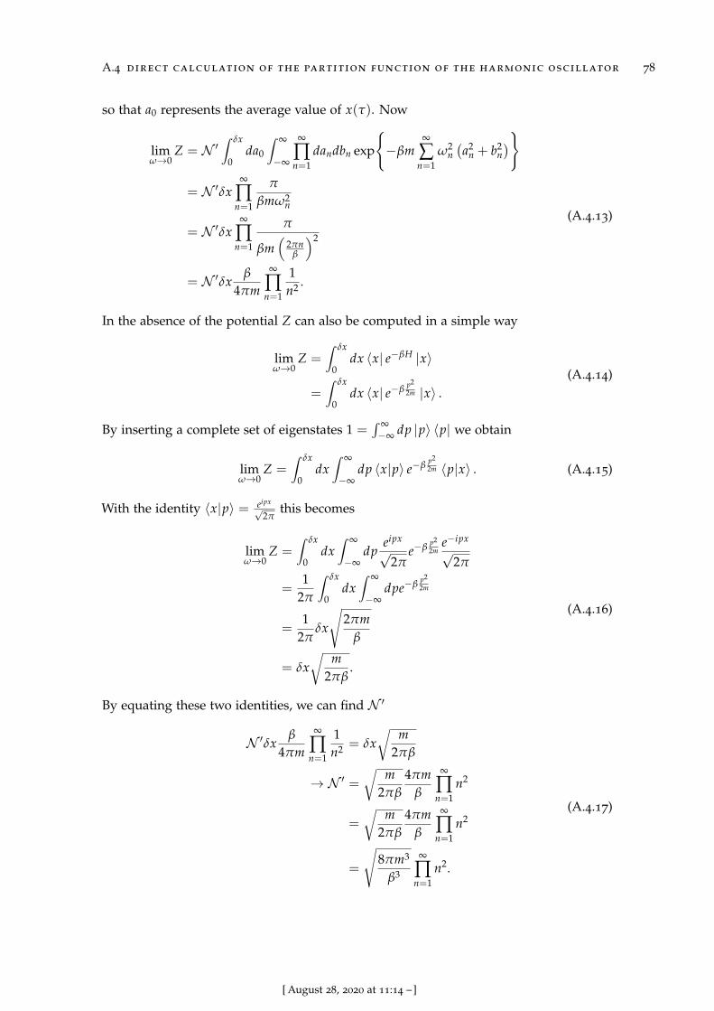
A.4 direct calculation of the partition function of the harmonic oscillator 78
so that a0 represents the average value of x(τ). Now
limω→0
Z = N ′∫ δx
0da0
∫ ∞
−∞
∞
∏n=1
dandbn exp
−βm
∞
∑n=1
ω2n(a2
n + b2n)
= N ′δx∞
∏n=1
π
βmω2n
= N ′δx∞
∏n=1
π
βm(
2πnβ
)2
= N ′δxβ
4πm
∞
∏n=1
1n2 .
(A.4.13)
In the absence of the potential Z can also be computed in a simple way
limω→0
Z =∫ δx
0dx 〈x| e−βH |x〉
=∫ δx
0dx 〈x| e−β
p22m |x〉 .
(A.4.14)
By inserting a complete set of eigenstates 1 =∫ ∞−∞ dp |p〉 〈p| we obtain
limω→0
Z =∫ δx
0dx∫ ∞
−∞dp 〈x|p〉 e−β
p22m 〈p|x〉 . (A.4.15)
With the identity 〈x|p〉 = eipx√
2πthis becomes
limω→0
Z =∫ δx
0dx∫ ∞
−∞dp
eipx√
2πe−β
p22m
e−ipx√
2π
=1
2π
∫ δx
0dx∫ ∞
−∞dpe−β
p22m
=1
2πδx
√2πm
β
= δx√
m2πβ
.
(A.4.16)
By equating these two identities, we can find N ′
N ′δxβ
4πm
∞
∏n=1
1n2 = δx
√m
2πβ
→ N ′ =
√m
2πβ
4πmβ
∞
∏n=1
n2
=
√m
2πβ
4πmβ
∞
∏n=1
n2
=
√8πm3
β3
∞
∏n=1
n2.
(A.4.17)
[ August 28, 2020 at 11:14 –]

A.4 direct calculation of the partition function of the harmonic oscillator 79
Therefore, Z can be rewritten as
Z =
√8πm3
β3
∞
∏n=1
n2 ×√
β3
32πm3
∞
∏n=1
1n2 csch(βω/2)
=12
csch(βω/2),
(A.4.18)
which is the same result as for the partition function in the canonical ensemble.
[ August 28, 2020 at 11:14 –]
B I B L I O G R A P H Y
[1] S. W. Hawking, “Black hole explosions?,” Nature 248 (1974) 30.
[2] S. W. Hawking, “Particle creation by black holes,” Commun. Math. Phys. 43 (1975)199.
[3] S. W. Hawking, “Black holes and thermodynamics,” Phys. Rev. D 13 (1976) 191.
[4] S. D. Mathur, “The information paradox: a pedagogical introduction,” Class. Quant.Grav. 26 (2009) 224001, arXiv:0909.1038 [hep-th].
[5] A. Almheiri, D. Marolf, J. Polchinski, and J. Sully, “Black holes: complementarity orfirewalls?,” JHEP 2 (2013) 62, arXiv:1207.3123 [hep-th].
[6] D. N. Page, “Information in black hole radiation,” Phys. Rev. Lett. 71 (1993) 3743,arXiv:hep-th/9306083 [hep-th].
[7] D. N. Page, “Time dependence of Hawking radiation entropy,” J. CosmologyAstropart. Phys. 09 (2013) 028, arXiv:1301.4995 [hep-th].
[8] A. Almheiri, T. Hartman, J. Maldacena, E. Shaghoulian, and A. Tajdini, “TheEntropy of Hawking Radiation,” arXiv:2006.06872 [hep-th].
[9] A. Almheiri, N. Engelhardt, D. Marolf, and H. Maxfield, “The entropy of bulkquantum fields and the entanglement wedge of an evaporating black hole,”arXiv:1905.08762 [hep-th].
[10] A. Almheiri, R. Mahajan, J. Maldacena, and Y. Zhao, “The Page curve of Hawkingradiation from semiclassical geometry,” arXiv:1908.10996 [hep-th].
[11] A. Almheiri, R. Mahajan, and J. Maldacena, “Islands outside the horizon,”arXiv:1910.11077 [hep-th].
[12] A. Almheiri, R. Mahajan, and J. E. Santos, “Entanglement islands in higherdimensions,” arXiv:1911.09666 [hep-th].
[13] A. Almheiri, T. Hartman, J. Maldacena, E. Shaghoulian, and A. Tajdini, “ReplicaWormholes and the Entropy of Hawking Radiation,” arXiv:1911.12333 [hep-th].
[14] G. Penington, “Entanglement Wedge Reconstruction and the Information Paradox,”arXiv:1905.08255 [hep-th].
[15] G. Penington, S. H. Shenker, D. Stanford, and Z. Yang, “Replica wormholes and theblack hole interior,” arXiv:1911.11977 [hep-th].
[16] D. Tong, “Lectures on String Theory,” arXiv:0908.0333 [hep-th].http://www.damtp.cam.ac.uk/user/tong/string.html.
80
[ August 28, 2020 at 11:14 –]
bibliography 81
[17] M. Headrick, “Lectures on entanglement entropy in field theory and holography,”arXiv:1907.08126 [hep-th].
[18] S. Ryu and T. Takayanagi, “Aspects of holographic entanglement entropy,” JHEP 8(2006) 045, arXiv:hep-th/0605073 [hep-th].
[19] M. van Raamsdonk, “Lectures on Gravity and Entanglement,” in New Frontiers inFields and Strings (TASI 2015), J. Polchinski, P. Vieira, and O. DeWolfe, eds.,p. 297–351. World Scientific, 2017. arXiv:1609.00026 [hep-th].
[20] G. T. Landi, “Quantum Statistical Mechanics and Condensed Matter Physics.”http://www.fmt.if.usp.br/∼gtlandi/courses/lecture-notes.pdf .
[21] D. Tong, “Statistical Field Theory.”http://www.damtp.cam.ac.uk/user/tong/sft.html.
[22] R. MacKenzie, “Path Integral Methods and Applications,” arXiv:quant-ph/0004090
[quant-ph].
[23] B. McKay, “Path Integrals in Quantum Mechanics.”http://www.math.utah.edu/∼mckay/qm.pdf .
[24] D. V. Pereplitsa, “Path Integrals in Quantum Mechanics.”http://web.mit.edu/dvp/www/Work/8.06/dvp-8.06-paper.pdf .
[25] K. Schulten, “Notes on Quantum Mechanics.”https://www.ks.uiuc.edu/Services/Class/PHYS480/qm PDF/QM Book.pdf .
[26] M. Strickland, Relativistic Quantum Field Theory, Volume 2; Path integral formalism.2019.
[27] G. Perez, “Quantum Mechanics II.”http://www.weizmann.ac.il/particle/perez/Courses/QMII17/PI lecture notes.pdf .
[28] J. Zinn-Justin, “Lecture 3: PATH INTEGRALS IN QUANTUM MECHANICS.”http://irfu.cea.fr/Phocea/file.php?class=page&file=678/QFT-IRFU2.pdf .
[29] R. Ratazzi, “The Path Integral approach to Quantum Mechanics Lecture Notes forQuantum Mechanics IV.” https://userswww.pd.infn.it/∼feruglio/rattazzi.pdf .
[30] A. Wipf, Statistical Approach to Quantum Field Theory, vol. 864. 2013.
[31] D. Tong, “Lectures on Quantum Field Theory.”http://www.damtp.cam.ac.uk/user/tong/qft.html.
[32] M. E. Peskin and D. V. Schroeder, An Introduction to Quantum Field Theory. 1995.
[33] A. Das, Field Theory: a Path Integral Approach (2nd Edition). 2006.
[34] G. Naber, “Classical Klein-Gordon Fields. Lagrangian and HamiltonianFormulations.”http://gregnaber.com/wp-content/uploads/The-Classical-Klein-Gordon-Field.pdf .
[35] P. J. Mulders, “Quantum Field Theory.”http://www.nat.vu.nl/∼mulders/QFT-0.pdf .
[ August 28, 2020 at 11:14 –]
bibliography 82
[36] J. L. Cardy, “Operator content of two-dimensional conformally invariant theories,”Nucl. Phys. B 270 (1986) 186.
[37] D. Wallace, “The case for black hole thermodynamics, Part II: statistical mechanics,”arXiv:1710.02725 [gr-qc].
[38] D. Harlow, “Jerusalem Lectures on Black Holes and Quantum Information,”arXiv:1409.1231 [hep-th].
[39] T. Hartman, “Lectures on Quantum Gravity and Black Holes.”http://www.hartmanhep.net/topics2015/gravity-lectures.pdf .
[40] T. Hartman, C. A. Keller, and B. Stoica, “Universal spectrum of 2d conformal fieldtheory in the large c limit,” JHEP 2014 (2014) 118, arXiv:1405.5137 [hep-th].
[41] M. Visser, Emergent Gravity in a Holographic Universe. PhD thesis, Universiteit vanAmsterdam, 2019. arXiv:1908.05469 [hep-th].https://hdl.handle.net/11245.1/3e860c5e-b60c-424d-84ba-1a47624f08c8.
[42] S. W. Hawking and D. N. Page, “Thermodynamics of black holes in anti-de Sitterspace,” Commun. Math. Phys. 87 (1982) 577.
[43] S. Winitzki, “Elementary Introduction to Quantum Fields in Curved Spacetime.”http://graduierten-kurse.physi.uni-heidelberg.de/SoSe2006/lectures/
Heidelberg 2006 presentations/Winitzki.pdf .
[44] K. Goto and Y. Kazama, “On the observer dependence of the Hilbert space near thehorizon of black holes,” Prog. Theor. Exp. Phys. 2019 (2019) 023B01, arXiv:1803.01672
[hep-th].
[45] N. D. Birrell and P. C. W. Davies, Quantum fields in curved space. CambridgeUniversity Press, 1982.
[46] M. Socolovsky, “Rindler Space and Unruh Effect,” arXiv:1304.2833 [gr-qc].
[47] N. Rahaman and I. Bischer, “The Unruh Effect.”https://www.thphys.uni-heidelberg.de/∼witkowski/curved/talk8.pdf .
[48] W. G. Unruh, “Notes on black-hole evaporation,” Phys. Rev. D 14 (1976) 870.
[49] C. Callan and F. Wilczek, “On geometric entropy,” Physics Letters B 333 (1994) 55,arXiv:hep-th/9401072 [hep-th].
[50] J. D. Bekenstein, “Black Holes and Entropy,” Phys. Rev. D 7 (1973) 2333.
[51] J. M. Bardeen, B. Carter, and S. W. Hawking, “The four laws of black holemechanics,” Commun. Math. Phys. 31 (1973) 161.
[52] L. Susskind and J. Uglum, “Black hole entropy in canonical quantum gravity andsuperstring theory,” Phys. Rev. D 50 (1994) 2700, arXiv:hep-th/9401070 [hep-th].
[53] V. P. Frolov, D. V. Fursaev, and A. I. Zelnikov, “Black hole entropy: Off shell versuson shell,” Phys. Rev. D 54 (1996) 2711, arXiv:hep-th/9512184 [hep-th].
[ August 28, 2020 at 11:14 –]

bibliography 83
[54] N. Engelhardt and A. C. Wall, “Quantum extremal surfaces: holographicentanglement entropy beyond the classical regime,” JHEP 1 (2015) 73,arXiv:1408.3203 [hep-th].
[55] S. Ryu and T. Takayanagi, “Holographic Derivation of Entanglement Entropy fromthe anti–de Sitter Space/Conformal Field Theory Correspondence,” Phys. Rev. Lett.96 (2006) 181602, arXiv:hep-th/0603001 [hep-th].
[56] V. E. Hubeny, M. Rangamani, and T. Takayanagi, “A covariant holographicentanglement entropy proposal,” JHEP 7 (2007) 062, arXiv:0705.0016 [hep-th].
[57] O. Aharony, S. S. Gubser, J. Maldacena, H. Ooguri, and Y. Oz, “Large N fieldtheories, string theory and gravity,” Phys. Rep. 323 (2000) 183, arXiv:hep-th/9905111
[hep-th].
[58] M. Natsuume, AdS/CFT Duality User Guide, vol. 903. 2015.
[59] P. Calabrese and J. Cardy, “Entanglement entropy and conformal field theory,”Journal of Physics A Mathematical General 42 (2009) 504005, arXiv:0905.4013
[cond-mat.stat-mech].
[60] M. Laine and A. Vuorinen, Basics of Thermal Field Theory, vol. 925. 2016.
[ August 28, 2020 at 11:14 –]


![Physics [CU MSc]](https://img.pdfslide.us/doc/110x75/55cf9c1d550346d033a8a8a7/physics-cu-msc.jpg)