Random entanglements

Jean-Luc Thiffeault

Department of MathematicsUniversity of Wisconsin – Madison

Joint work with Marko Budisic & Huanyu Wen

Applied Mathematics Seminar, Stanford University

Stanford, CA, 20 November 2014

Supported by NSF grant CMMI-1233935

1 / 36

Complex entanglements areeverywhere

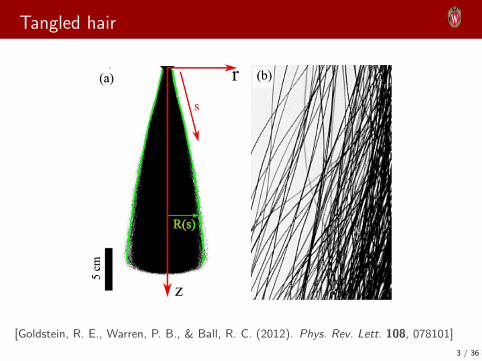
Tangled hair

[Goldstein, R. E., Warren, P. B., & Ball, R. C. (2012). Phys. Rev. Lett. 108, 078101]

3 / 36

Tangled hagfish slime

Slime secreted by hagfish ismade of microfibers.

The quality of entanglementdetermines the materialproperties (rheology) of theslime.

[Fudge, D. S., Levy, N., Chiu, S., & Gosline, J. M. (2005). J. Exp. Biol. 208, 4613–4625]

4 / 36

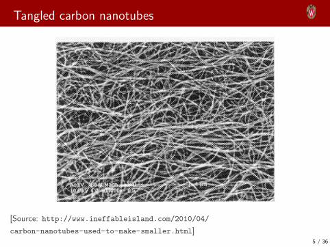
Tangled carbon nanotubes

[Source: http://www.ineffableisland.com/2010/04/

carbon-nanotubes-used-to-make-smaller.html]5 / 36

Tangled magnetic fields

[Source: http://www.maths.dundee.ac.uk/mhd/]

6 / 36

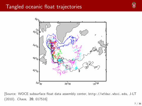
Tangled oceanic float trajectories

72 oW

54 oW 36

oW 18

oW

0o

42 oN

48 oN

54 oN

60 oN

66 oN

[Source: WOCE subsurface float data assembly center, http://wfdac.whoi.edu, J-LT

(2010). Chaos, 20, 017516]7 / 36

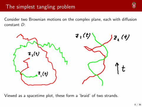
The simplest tangling problem

Consider two Brownian motions on the complex plane, each with diffusionconstant D:

Viewed as a spacetime plot, these form a ‘braid’ of two strands.

8 / 36

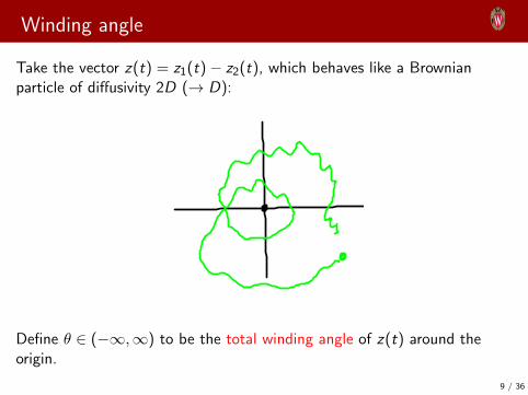
Winding angle

Take the vector z(t) = z1(t)− z2(t), which behaves like a Brownianparticle of diffusivity 2D (→ D):

Define θ ∈ (−∞,∞) to be the total winding angle of z(t) around theorigin.

9 / 36

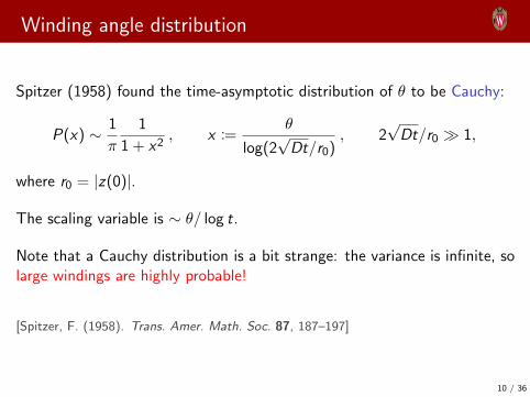
Winding angle distribution

Spitzer (1958) found the time-asymptotic distribution of θ to be Cauchy:

P(x) ∼ 1

π

1

1 + x2, x :=

θ

log(2√Dt/r0)

, 2√Dt/r0 � 1,

where r0 = |z(0)|.

The scaling variable is ∼ θ/ log t.

Note that a Cauchy distribution is a bit strange: the variance is infinite, solarge windings are highly probable!

[Spitzer, F. (1958). Trans. Amer. Math. Soc. 87, 187–197]

10 / 36

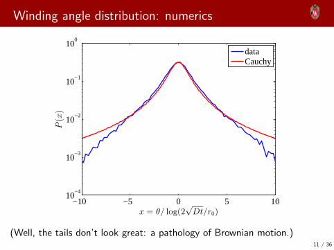
Winding angle distribution: numerics

−10 −5 0 5 1010

−4

10−3

10−2

10−1

100

x = θ/ log(2√

Dt/r0)

P(x)

dataCauchy

(Well, the tails don’t look great: a pathology of Brownian motion.)11 / 36

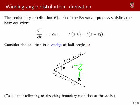
Winding angle distribution: derivation

The probability distribution P(z , t) of the Brownian process satisfies theheat equation:

∂P

∂t= D∆P, P(z , 0) = δ(z − z0).

Consider the solution in a wedge of half-angle α:

(Take either reflecting or absorbing boundary condition at the walls.)

12 / 36

Winding angle distribution: derivation (cont’d)

The solution is standard, but now take the wedge angle α to ∞ (!):

P(z , t) =1

2πDte−(r2+r2

0 )/4Dt

∫ ∞0

cos ν(θ − θ0) Iν( r r0

2Dt

)dν

where Iν is a modified Bessel function of the first kind, and r , θ are thepolar coordinates of z = x + iy .

For large t this recovers the Cauchy distribution.

Key point: by allowing the wedge angle to infinity, we are using Riemannsheets to keep track of the winding angle.

13 / 36

Related example: Brownian motion on the torus

A Brownian motion on a torus can wind around the two periodic directions:

What is the asymptotic distribution of windings?

Mathematically, we are asking what is the homology class of the motion?

14 / 36

Torus: universal cover

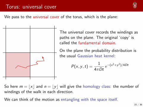
We pass to the universal cover of the torus, which is the plane:

The universal cover records the windings aspaths on the plane. The original ‘copy’ iscalled the fundamental domain.

On the plane the probability distribution isthe usual Gaussian heat kernel:

P(x , y , t) =1

4πDte−(x2+y2)/4Dt

So here m = bxc and n = byc will give the homology class: the number ofwindings of the walk in each direction.

We can think of the motion as entangling with the space itself.15 / 36

Brownian motion on the double-torus

On a genus two surface (double-torus):

Same question: what is the entanglement of the motion with the spaceafter a long time?

Now homology classes are not enough, since the associated universal coverhas a non-Abelian group of deck transformations. In other words, theorder of going around the holes matters!

The non-Abelian case involves homotopy classes.

16 / 36

The ‘stop sign’ representation of the double-torus

a

a

b

b

c

c

d

d

(Identify edges,

respecting

orientation.)

Problem: can’t tile the plane with this!17 / 36

Universal cover of the double-torus

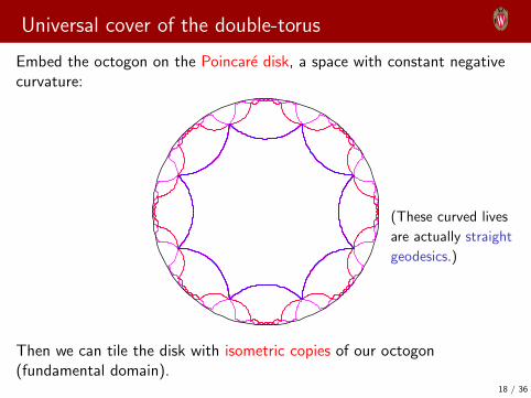
Embed the octogon on the Poincare disk, a space with constant negativecurvature:

(These curved lives

are actually straight

geodesics.)

Then we can tile the disk with isometric copies of our octogon(fundamental domain).

18 / 36

Heat kernel on the Poincare disk

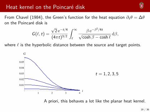
From Chavel (1984), the Green’s function for the heat equation ∂tθ = ∆θon the Poincare disk is

G (`, t) =

√2 e−t/4

(4πt)3/2

∫ ∞`

β e−β2/4t

√coshβ − cosh `

dβ,

where ` is the hyperbolic distance between the source and target points.

1 2 3 4l

0.01

0.02

0.03

0.04

0.05

G

t = 1, 2, 3, 5

A priori, this behaves a lot like the planar heat kernel.

19 / 36

Squared-displacement on the Poincare disk

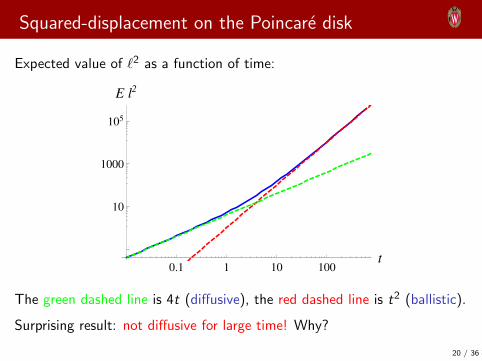
Expected value of `2 as a function of time:

0.1 1 10 100t

10

1000

105

E l2

The green dashed line is 4t (diffusive), the red dashed line is t2 (ballistic).

Surprising result: not diffusive for large time! Why?

20 / 36

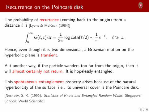
Recurrence on the Poincare disk

The probability of recurrence (coming back to the origin) from adistance ` is [Lyons & McKean (1984)]∫ ∞

0G (`, t)dt =

1

2πlog coth(`/2) ∼ 1

πe−`, `� 1.

Hence, even though it is two-dimensional, a Brownian motion on thehyperbolic plane is transient.

Put another way, if the particle wanders too far from the origin, then itwill almost certainly not return. It is hopelessly entangled.

This spontaneous entanglement property arises because of the naturalhyperbolicity of the surface, i.e., its universal cover is the Poincare disk.

[Nechaev, S. K. (1996). Statistics of Knots and Entangled Random Walks. Singapore;

London: World Scientific]

21 / 36

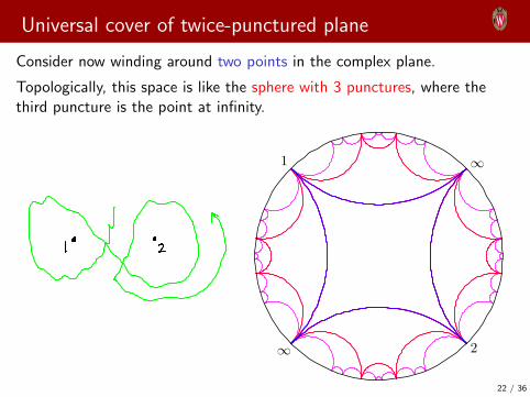
Universal cover of twice-punctured plane

Consider now winding around two points in the complex plane.

Topologically, this space is like the sphere with 3 punctures, where thethird puncture is the point at infinity.

∞

∞ 2

1

22 / 36

Cayley graph of free group

We really only care about which‘copy’ of the fundamental domainwe’re in. Can use a tree to recordthis.

The history of a path is encodedin a ‘word’ in the letters a, b,a−1, b−1.

(Free group with two generators.)

[Source: Wikipedia]

23 / 36

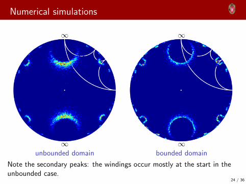
Numerical simulations

∞

∞unbounded domain

∞

∞bounded domain

Note the secondary peaks: the windings occur mostly at the start in theunbounded case.

24 / 36

Some references

Many people have worked on aspects of this problem:

• [Spitzer (1958); Durrett (1982); Messulam & Yor (1982); Berger (1987); Shi

(1998)] winding of Brownian motion around a point in R2.

• [Berger & Roberts (1988); Belisle (1989); Belisle & Faraway (1991); Rudnick &

Hu (1987)] winding of random walk around a point.

• [Drossel & Kardar (1996); Grosberg & Frisch (2003)] finite obstacle, closeddomain.

• [Ito & McKean (1974); McKean (1969); Lyons & McKean (1984)]

doubly-punctured plane.

• [McKean & Sullivan (1984)] three-punctured sphere.

• [Pitman & Yor (1986, 1989)] more points.

• [Watanabe (2000)] Riemann surfaces.

• [Nechaev (1988)] lattice of obstacles.

• [Nechaev (1996); Revuz & Yor (1999)] comprehensive books.

25 / 36

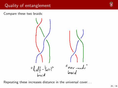
Quality of entanglement

Compare these two braids:

Repeating these increases distance in the universal cover. . .26 / 36

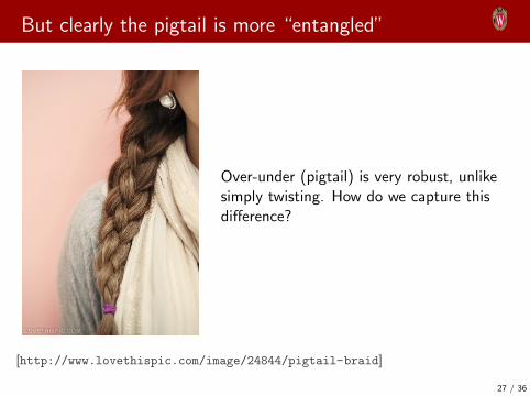
But clearly the pigtail is more “entangled”

Over-under (pigtail) is very robust, unlikesimply twisting. How do we capture thisdifference?

[http://www.lovethispic.com/image/24844/pigtail-braid]

27 / 36

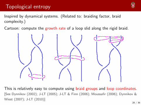
Topological entropy

Inspired by dynamical systems. (Related to: braiding factor, braidcomplexity.)

Cartoon: compute the growth rate of a loop slid along the rigid braid.

This is relatively easy to compute using braid groups and loop coordinates.[See Dynnikov (2002); J-LT (2005); J-LT & Finn (2006); Moussafir (2006); Dynnikov &

Wiest (2007); J-LT (2010)]28 / 36

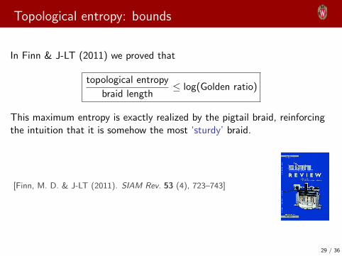
Topological entropy: bounds

In Finn & J-LT (2011) we proved that

topological entropy

braid length≤ log(Golden ratio)

This maximum entropy is exactly realized by the pigtail braid, reinforcingthe intuition that it is somehow the most ‘sturdy’ braid.

[Finn, M. D. & J-LT (2011). SIAM Rev. 53 (4), 723–743]

29 / 36

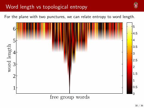
Word length vs topological entropy

For the plane with two punctures, we can relate entropy to word length.

free group words

word

length

1

2

3

4

5

6

0

0.5

1

1.5

2

2.5

3

3.5

4

4.5

5

30 / 36

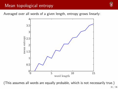
Mean topological entropy

Averaged over all words of a given length, entropy grows linearly:

0 5 10 150

0.5

1

1.5

2

2.5

3

3.5

4

word length

meanentropy

(This assumes all words are equally probable, which is not necessarily true.)31 / 36

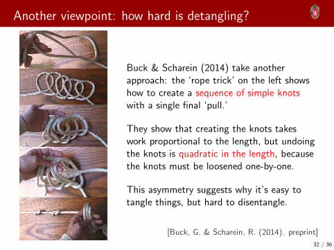
Another viewpoint: how hard is detangling?

Buck & Scharein (2014) take anotherapproach: the ‘rope trick’ on the left showshow to create a sequence of simple knotswith a single final ‘pull.’

They show that creating the knots takeswork proportional to the length, but undoingthe knots is quadratic in the length, becausethe knots must be loosened one-by-one.

This asymmetry suggests why it’s easy totangle things, but hard to disentangle.

[Buck, G. & Scharein, R. (2014). preprint]

32 / 36

Conclusions & outlook

• Entanglement at confluence of dynamics, probability, topology, andcombinatorics.

• Instead of Brownian motion, can use orbits from a dynamical system.This yields dynamical information.

• More generally, study random processes on configuration spaces ofsets of points (also finite size objects).

• Other applications: Crowd dynamics (Ali, 2013), granular media(Puckett et al., 2012).

• With Michael Allshouse: develop tools for analyzing orbit data fromthis topological viewpoint (Allshouse & J-LT, 2012).

• With Tom Peacock and Margaux Filippi: apply to orbits in a fluiddynamics experiments.

33 / 36

References I

Ali, S. (2013). In: IEEE International Conference on Computer Vision (ICCV) pp. 1097–1104, :.

Allshouse, M. R. & J-LT (2012). Physica D, 241 (2), 95–105.

Belisle, C. (1989). Ann. Prob. 17 (4), 1377–1402.

Belisle, C. & Faraway, J. (1991). J. Appl. Prob. 28 (4), 717–726.

Berger, M. A. (1987). J. Phys. A, 20, 5949–5960.

Berger, M. A. & Roberts, P. H. (1988). Adv. Appl. Prob. 20 (2), 261–274.

Buck, G. & Scharein, R. (2014). preprint.

Chavel, I. (1984). Eigenvalues in Riemannian Geometry. Orlando: Academic Press.

Drossel, B. & Kardar, M. (1996). Phys. Rev. E, 53 (6), 5861–5871.

Durrett, R. (1982). Ann. Prob. 10 (1), 244–246.

Dynnikov, I. A. (2002). Russian Math. Surveys, 57 (3), 592–594.

Dynnikov, I. A. & Wiest, B. (2007). Journal of the European Mathematical Society, 9 (4),801–840.

Finn, M. D. & J-LT (2011). SIAM Rev. 53 (4), 723–743.

Fudge, D. S., Levy, N., Chiu, S., & Gosline, J. M. (2005). J. Exp. Biol. 208, 4613–4625.

Goldstein, R. E., Warren, P. B., & Ball, R. C. (2012). Phys. Rev. Lett. 108, 078101.

Grosberg, A. & Frisch, H. (2003). J. Phys. A, 36 (34), 8955–8981.

34 / 36

References II

Ito, K. & McKean, H. P. (1974). Diffusion processes and their sample paths. Berlin: Springer.

Lyons, T. J. & McKean, H. P. (1984). Adv. Math. 51, 212–225.

McKean, H. P. (1969). Stochastic Integrals. New York: Academic Press.

McKean, H. P. & Sullivan, D. (1984). Adv. Math. 51, 203–211.

Messulam, P. & Yor, M. (1982). J. London Math. Soc. (2), 26, 348–364.

Moussafir, J.-O. (2006). Func. Anal. and Other Math. 1 (1), 37–46.

Nechaev, S. K. (1988). J. Phys. A, 21, 3659–3671.

Nechaev, S. K. (1996). Statistics of Knots and Entangled Random Walks. Singapore; London:World Scientific.

Pitman, J. & Yor, M. (1986). Ann. Prob. 14 (3), 733–779.

Pitman, J. & Yor, M. (1989). Ann. Prob. 17 (3), 965–1011.

Puckett, J. G., Lechenault, F., Daniels, K. E., & J-LT (2012). Journal of Statistical Mechanics:Theory and Experiment, 2012 (6), P06008.

Revuz, D. & Yor, M. (1999). Continuous Martingales and Brownian motion. Berlin: Springer,third edition.

Rudnick, J. & Hu, Y. (1987). J. Phys. A, 20, 4421–4438.

Shi, Z. (1998). Ann. Prob. 26 (1), 112–131.

Spitzer, F. (1958). Trans. Amer. Math. Soc. 87, 187–197.

35 / 36

References III

J-LT (2005). Phys. Rev. Lett. 94 (8), 084502.

J-LT (2010). Chaos, 20, 017516.

J-LT & Finn, M. D. (2006). Phil. Trans. R. Soc. Lond. A, 364, 3251–3266.

Watanabe, S. (2000). Acta Applicandae Mathematicae, 63, 441–464.

36 / 36