Growth of loops Coding of loops LCS Conclusions References

Topological tools for trajectory data analysis

Jean-Luc Thiffeault1 Michael Allshouse2

1Department of MathematicsUniversity of Wisconsin – Madison

2Department of PhysicsUniversity of Texas – Austin

SJTU International Forum on Mathematics10 January 2014

Supported by NSF grants DMS-0806821 and CMMI-1233935

1 / 25

Growth of loops Coding of loops LCS Conclusions References

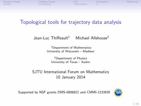
Sparse trajectories and material loops

−2 −1 0 1 2

−2.5

−2

−1.5

−1

−0.5

0

0.5

1

1.5

2

2.5

x

y

How do we efficiently detect trajectories that ‘bunch’ together?

Growth of curves also studied in LCS context by Haller &Beron-Vera (2012).[movie 1]

2 / 25

Growth of loops Coding of loops LCS Conclusions References

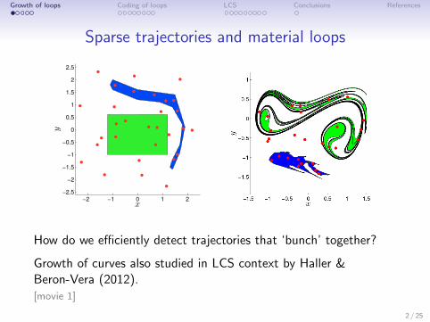
Mathematical background: Punctured disks

Low-dimensional topologists have long studied transformations ofsurfaces such as the punctured disk:

The central object of study is the homeomorphism: a continuous,invertible transformation whose inverse is also continuous.

For instance, this is a model of a two-dimensional vat of viscousfluid with stirring rods.

3 / 25

Growth of loops Coding of loops LCS Conclusions References

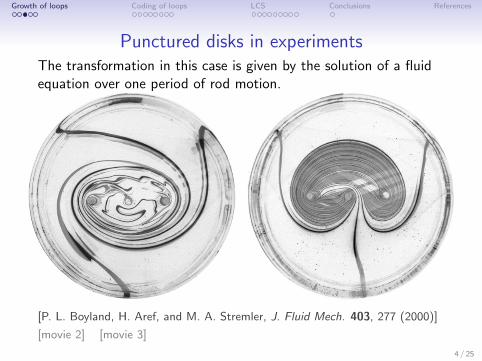
Punctured disks in experimentsThe transformation in this case is given by the solution of a fluidequation over one period of rod motion.

[P. L. Boyland, H. Aref, and M. A. Stremler, J. Fluid Mech. 403, 277 (2000)]

[movie 2] [movie 3]

4 / 25

Growth of loops Coding of loops LCS Conclusions References

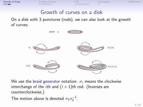
Growth of curves on a diskOn a disk with 3 punctures (rods), we can also look at the growthof curves:

�1

�1�2-1

�1�2-1�1

�2-1�1�2

-1�1

initial

We use the braid generator notation: σi means the clockwiseinterchange of the ith and (i + 1)th rod. (Inverses arecounterclockwise.)

The motion above is denoted σ1σ−12 .

5 / 25

Growth of loops Coding of loops LCS Conclusions References

Growth of curves on a disk (2)

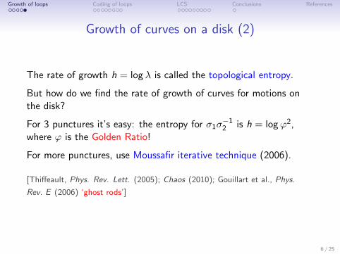
The rate of growth h = log λ is called the topological entropy.

But how do we find the rate of growth of curves for motions onthe disk?

For 3 punctures it’s easy: the entropy for σ1σ−12 is h = logϕ2,

where ϕ is the Golden Ratio!

For more punctures, use Moussafir iterative technique (2006).

[Thiffeault, Phys. Rev. Lett. (2005); Chaos (2010); Gouillart et al., Phys.

Rev. E (2006) ‘ghost rods’]

6 / 25

Growth of loops Coding of loops LCS Conclusions References

Iterating a loop

It is well-known that the entropy can be obtained by applying themotion of the punctures to a closed curve (loop) repeatedly, andmeasuring the growth of the length of the loop (Bowen, 1978).

The problem is twofold:

1. Need to keep track of the loop, since its length is growingexponentially;

2. Need a simple way of transforming the loop according to themotion of the punctures.

However, simple closed curves are easy objects to manipulate in2D. Since they cannot self-intersect, we can describe themtopologically with very few numbers.

7 / 25

Growth of loops Coding of loops LCS Conclusions References

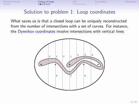
Solution to problem 1: Loop coordinates

What saves us is that a closed loop can be uniquely reconstructedfrom the number of intersections with a set of curves. For instance,the Dynnikov coordinates involve intersections with vertical lines:

2

30 0

14 4 4

2 2

8 / 25

Growth of loops Coding of loops LCS Conclusions References

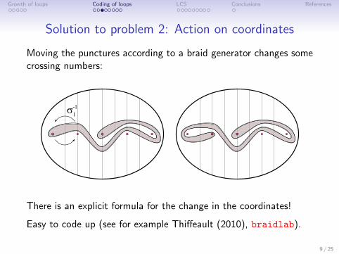
Solution to problem 2: Action on coordinates

Moving the punctures according to a braid generator changes somecrossing numbers:

�1-1

There is an explicit formula for the change in the coordinates!

Easy to code up (see for example Thiffeault (2010), braidlab).

9 / 25

Growth of loops Coding of loops LCS Conclusions References

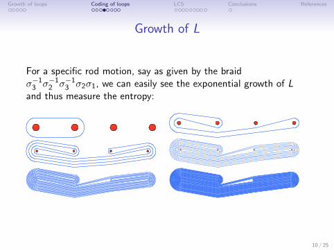
Growth of L

For a specific rod motion, say as given by the braidσ−1

3 σ−12 σ−1

3 σ2σ1, we can easily see the exponential growth of Land thus measure the entropy:

10 / 25

Growth of loops Coding of loops LCS Conclusions References

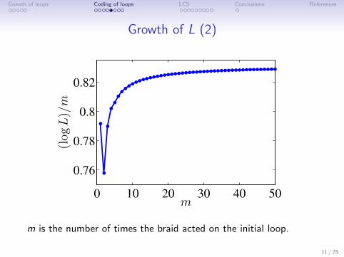
Growth of L (2)

0 10 20 30 40 50

0.76

0.78

0.8

0.82

m

(logL)/m

m is the number of times the braid acted on the initial loop.

11 / 25

Growth of loops Coding of loops LCS Conclusions References

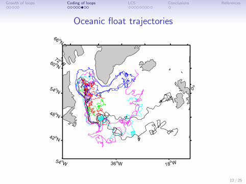
Oceanic float trajectories

72 oW

54 oW 36

oW 18

oW

0o

42 oN

48 oN

54 oN

60 oN

66 oN

12 / 25

Growth of loops Coding of loops LCS Conclusions References

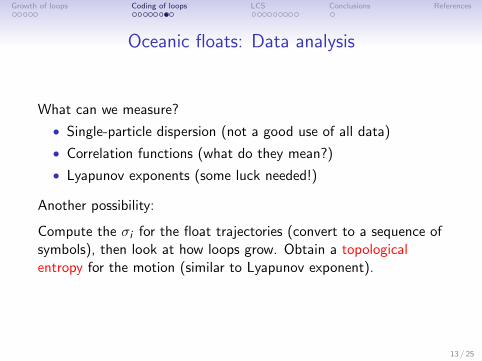
Oceanic floats: Data analysis

What can we measure?

• Single-particle dispersion (not a good use of all data)

• Correlation functions (what do they mean?)

• Lyapunov exponents (some luck needed!)

Another possibility:

Compute the σi for the float trajectories (convert to a sequence ofsymbols), then look at how loops grow. Obtain a topologicalentropy for the motion (similar to Lyapunov exponent).

13 / 25

Growth of loops Coding of loops LCS Conclusions References

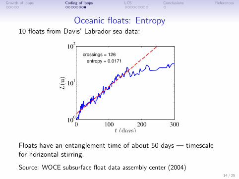
Oceanic floats: Entropy10 floats from Davis’ Labrador sea data:

0 100 200 30010

0

101

102

t (days)

L(u

) entropy = 0.0171

crossings = 126

Floats have an entanglement time of about 50 days — timescalefor horizontal stirring.

Source: WOCE subsurface float data assembly center (2004)14 / 25

Growth of loops Coding of loops LCS Conclusions References

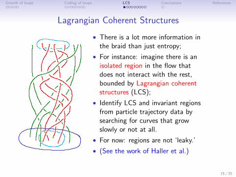
Lagrangian Coherent Structures

• There is a lot more information inthe braid than just entropy;

• For instance: imagine there is anisolated region in the flow thatdoes not interact with the rest,bounded by Lagrangian coherentstructures (LCS);

• Identify LCS and invariant regionsfrom particle trajectory data bysearching for curves that growslowly or not at all.

• For now: regions are not ‘leaky.’

• (See the work of Haller et al.)

15 / 25

Growth of loops Coding of loops LCS Conclusions References

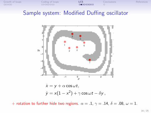
Sample system: Modified Duffing oscillator

−2 −1 0 1 2 3−4

−3

−2

−1

0

1

2

3

x

y

1

2

3

4

5

6

7

x = y + α cosωt,

y = x(1 − x2) + γ cosωt − δy ,

+ rotation to further hide two regions. α = .1, γ = .14, δ = .08, ω = 1.

16 / 25

Growth of loops Coding of loops LCS Conclusions References

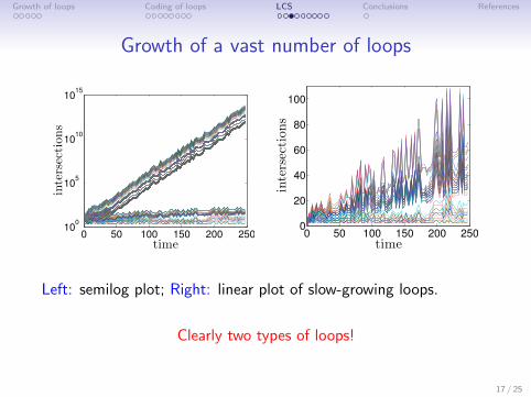
Growth of a vast number of loops

0 50 100 150 200 25010

0

105

1010

1015

time

intersections

0 50 100 150 200 2500

20

40

60

80

100

time

intersections

Left: semilog plot; Right: linear plot of slow-growing loops.

Clearly two types of loops!

17 / 25

Growth of loops Coding of loops LCS Conclusions References

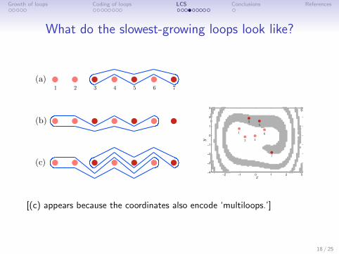
What do the slowest-growing loops look like?

(a)

(b)

(c)

1 2 3 4 5 6 7

−2 −1 0 1 2 3−4

−3

−2

−1

0

1

2

3

x

y

1

2

3

4

5

6

7

[(c) appears because the coordinates also encode ‘multiloops.’]

18 / 25

Growth of loops Coding of loops LCS Conclusions References

Computational complexity

Here’s the bad news:

• There are an infinite number of loops to consider.

• But we don’t really expect hyper-convoluted initial loops (nordo we care so much about those).

• Even if we limit ourselves to loops with Dynnikov coordinatesbetween −1 and 1, this is still 32n−4 loops.

• This is too many. . . can only treat about 10–11 trajectoriesusing this direct method.

19 / 25

Growth of loops Coding of loops LCS Conclusions References

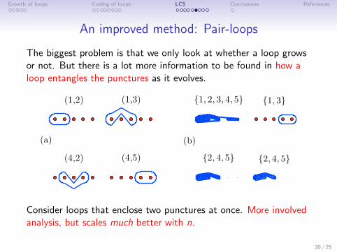
An improved method: Pair-loops

The biggest problem is that we only look at whether a loop growsor not. But there is a lot more information to be found in how aloop entangles the punctures as it evolves.

(1,2)

(a)

(1,3)

(4,2) (4,5)

{1, 2, 3, 4, 5}

(b)

{1, 3}

{2, 4, 5} {2, 4, 5}

Consider loops that enclose two punctures at once. More involvedanalysis, but scales much better with n.

20 / 25

Growth of loops Coding of loops LCS Conclusions References

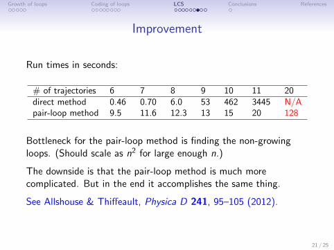
Improvement

Run times in seconds:

# of trajectories 6 7 8 9 10 11 20direct method 0.46 0.70 6.0 53 462 3445 N/Apair-loop method 9.5 11.6 12.3 13 15 20 128

Bottleneck for the pair-loop method is finding the non-growingloops. (Should scale as n2 for large enough n.)

The downside is that the pair-loop method is much morecomplicated. But in the end it accomplishes the same thing.

See Allshouse & Thiffeault, Physica D 241, 95–105 (2012).

21 / 25

Growth of loops Coding of loops LCS Conclusions References

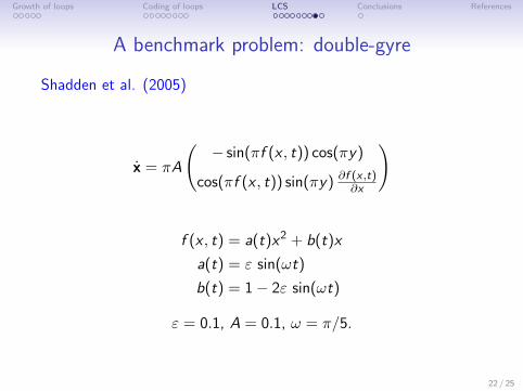
A benchmark problem: double-gyre

Shadden et al. (2005)

x = πA

( − sin(πf (x , t)) cos(πy)

cos(πf (x , t)) sin(πy) ∂f (x ,t)∂x

)

f (x , t) = a(t)x2 + b(t)x

a(t) = ε sin(ωt)

b(t) = 1 − 2ε sin(ωt)

ε = 0.1, A = 0.1, ω = π/5.

22 / 25

Growth of loops Coding of loops LCS Conclusions References

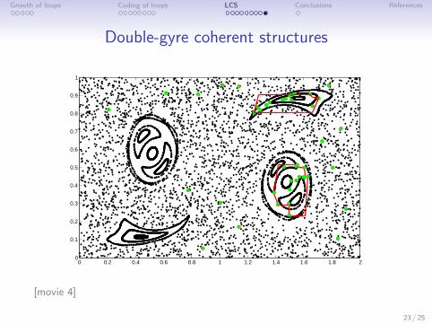
Double-gyre coherent structures

0 0.2 0.4 0.6 0.8 1 1.2 1.4 1.6 1.8 20

0.1

0.2

0.3

0.4

0.5

0.6

0.7

0.8

0.9

1

[movie 4]

23 / 25

Growth of loops Coding of loops LCS Conclusions References

Conclusions

• Having rods undergo ‘braiding’ motion guarantees a minimalamount of entropy (stretching of material lines);

• This idea can also be used on fluid particles to estimateentropy;

• Need a way to compute entropy fast: loop coordinates;

• There is a lot more information in this braid: extract it!(coherent structures);

• However: Difficult to find an appropriate data set.

• We’re investigating the limits of the approach (how manytrajectories, how long).

• We’re developing Matlab tools — braidlab.

• Also applicable to granular media Puckett et al. (2012).

• See Thiffeault (2005, 2010) and Allshouse & Thiffeault(2012).

24 / 25

Growth of loops Coding of loops LCS Conclusions References

ReferencesAllshouse, M. R. & Thiffeault, J.-L. 2012 Detecting Coherent Structures Using Braids. Physica D 241, 95–105.

Bestvina, M. & Handel, M. 1995 Train-Tracks for Surface Homeomorphisms. Topology 34, 109–140.

Binder, B. J. & Cox, S. M. 2008 A Mixer Design for the Pigtail Braid. Fluid Dyn. Res. 49, 34–44.

Bowen, R. 1978 Entropy and the fundamental group. In Structure of Attractors, volume 668 of Lecture Notes inMath., pp. 21–29. New York: Springer.

Boyland, P. L. 1994 Topological methods in surface dynamics. Topology Appl. 58, 223–298.

Boyland, P. L., Aref, H. & Stremler, M. A. 2000 Topological fluid mechanics of stirring. J. Fluid Mech. 403,277–304.

Boyland, P. L., Stremler, M. A. & Aref, H. 2003 Topological fluid mechanics of point vortex motions. Physica D175, 69–95.

Dynnikov, I. A. 2002 On a Yang–Baxter map and the Dehornoy ordering. Russian Math. Surveys 57, 592–594.

Finn, M. D. & Thiffeault, J.-L. 2011 Topological optimisation of rod-stirring devices. SIAM Rev. 53, 723–743.

Gouillart, E., Finn, M. D. & Thiffeault, J.-L. 2006 Topological Mixing with Ghost Rods. Phys. Rev. E 73, 036311.

Hall, T. & Yurttas, S. O. 2009 On the Topological Entropy of Families of Braids. Topology Appl. 156, 1554–1564.

Haller, G. & Beron-Vera, F. J.. 2012 Geodesic theory of transport barriers in two-dimensional flows. Physica D,submitted

Kolev, B. 1989 Entropie topologique et representation de Burau. C. R. Acad. Sci. Ser. I 309, 835–838. Englishtranslation at arXiv:math.DS/0304105.

Moussafir, J.-O. 2006 On the Entropy of Braids. Func. Anal. and Other Math. 1, 43–54. arXiv:math.DS/0603355.

Puckett, J. G., Lechenault, F., Daniels, K. E. & Thiffeault, J.-L. 2012 Trajectory entanglement in dense granularmaterials. arXiv:1202.5243.

Thiffeault, J.-L. 2005 Measuring Topological Chaos. Phys. Rev. Lett. 94, 084502.

Thiffeault, J.-L. 2010 Braids of entangled particle trajectories. Chaos, 20, 017516.

Thiffeault, J.-L. & Finn, M. D. 2006 Topology, Braids, and Mixing in Fluids. Phil. Trans. R. Soc. Lond. A 364,3251–3266.

Thurston, W. P. 1988 On the geometry and dynamics of diffeomorphisms of surfaces. Bull. Am. Math. Soc. 19,417–431.

25 / 25