DEPARTMENT OF ECONOMICS

WORKING PAPER

2005

Department of Economics Tufts University

Medford, MA 02155 (617) 627 – 3560

http://ase.tufts.edu/econ

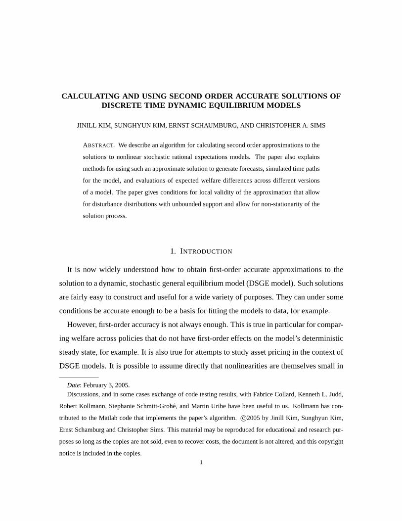
CALCULATING AND USING SECOND ORDER ACCURATE SOLUTIONS OFDISCRETE TIME DYNAMIC EQUILIBRIUM MODELS

JINILL KIM, SUNGHYUN KIM, ERNST SCHAUMBURG, AND CHRISTOPHER A. SIMS

ABSTRACT. We describe an algorithm for calculating second order approximations to the

solutions to nonlinear stochastic rational expectations models. The paper also explains

methods for using such an approximate solution to generate forecasts, simulated time paths

for the model, and evaluations of expected welfare differences across different versions

of a model. The paper gives conditions for local validity of the approximation that allow

for disturbance distributions with unbounded support and allow for non-stationarity of the

solution process.

1. INTRODUCTION

It is now widely understood how to obtain first-order accurate approximations to the

solution to a dynamic, stochastic general equilibrium model (DSGE model). Such solutions

are fairly easy to construct and useful for a wide variety of purposes. They can under some

conditions be accurate enough to be a basis for fitting the models to data, for example.

However, first-order accuracy is not always enough. This is true in particular for compar-

ing welfare across policies that do not have first-order effects on the model’s deterministic

steady state, for example. It is also true for attempts to study asset pricing in the context of

DSGE models. It is possible to assume directly that nonlinearities are themselves small in

Date: February 3, 2005.

Discussions, and in some cases exchange of code testing results, with Fabrice Collard, Kenneth L. Judd,

Robert Kollmann, Stephanie Schmitt-Grohe, and Martin Uribe have been useful to us. Kollmann has con-

tributed to the Matlab code that implements the paper’s algorithm.c©2005 by Jinill Kim, Sunghyun Kim,

Ernst Schamburg and Christopher Sims. This material may be reproduced for educational and research pur-

poses so long as the copies are not sold, even to recover costs, the document is not altered, and this copyright

notice is included in the copies.1

SECOND ORDER SOLUTION 2

certain dimensions as a justification for use of first-order approximations in these contexts;

Woodford(2002) is an example of making the necessary auxiliary assumptions explicit.

But the usual reliance on local approximation being generally locally accurate does not

apply to these contexts.

It is therefore of some interest to have an algorithm available that will produce second-

order accurate approximations to the solutions to DSGE’s from a straightforward second-

order expansion of the model’s equilibrium equations, and this is an active area of recent

research.

Kenneth Judd pioneered this field by using perturbation methods in solving various types

of economic models1. Jin and Judd(2002) describe how to compute approximations of arbi-

trary order in discrete-time rational expectations models. They aim at providing a complete

set of regularity conditions justifying the local approximations, and they discuss methods

for checking the validity of the approximations. Others also have studied perturbation

methods of higher than first order includingCollard and Juillard(2000), Anderson and

Levin (2002), andSchmitt-Grohe and Uribe(2002).

Kim and Kim (2003a) andSutherland(2002) have developed a bias correction method

that produces the same results as the second order perturbation method for certain welfare

calculations, while requiring less computational effort than a full perturbation solution.

Several papers have applied the second-order perturbation method to dynamic general

equilibrium models.Kim and Kim (2003b) used the second-order solution method to ana-

lyze welfare effects of tax policies in a two-country framework. In particular, they calculate

the optimal degree of response for various tax rates to TFP shocks faced by each country.

Welfare gains of tax policies are measured by conditional welfare changes from the bench-

mark case.Kollmann(2002) has analyzed the welfare effects of monetary policies in open

economies using the software that has been developed along with this paper, andBergin

and Tchakarov(2002) have used it to examine the welfare effects of exchange rate risk.

1Judd(1998). For continuous time models seeGaspar and Judd(1997) as well.

SECOND ORDER SOLUTION 3

This paper describes the algorithm for computing a second order approximation and

shows how to apply it to calculating forecasts and impulse responses in dynamic models

and to evaluating welfare in DSGE models. It points out some necessary regularity con-

ditions for application of the method and discusses the sense in which the approximate

solutions are locally accurate.

While much of the paper parallels others in this rapidly growing literature, this paper

makes some new contributions. The rest of the literature in most cases begins from a for-

mulation of the problem in which a partition of variables in the model into “states” and

“controls” or “co-states” is assumed known. While in smaller models such a partition is

often obvious, in larger models it can be unclear how to partition the variables into states

and controls. The Matlab programgensys.m , implementing the approach described in

Sims(2001), accepts model specifications that do not partition the variable list into pre-

determined and non-predetermined variables; instead it partitions disturbances into prede-

termined and non-predetermined categories. This approach is more natural in systems de-

rived from equilibrium models, in which equation disturbances often fall neatly into these

categories. In such models translating the list of predetermined disturbances into a corre-

sponding list of predetermined variables (or, where necessary, new predetermined variables

that are linear combinations of the original model’s variables) may not be easy. This paper

extends that approach to second-order approximations.2

The “state-free” approach ofgensys.m has the disadvantage that its output, while com-

pletely characterizing the dynamics in terms of the original variables, includes only its own

artificial decomposition into states and co-states, which may be opaque. For some purposes

it is important to have an intuitively appealing decomposition into states and co-states. We

discuss how to do this, with the aid of another program,gstate.m , that uses the output

of gensys.m or gensys2.m to test proposed state vectors and and to provide guidance

as to what a valid state vector must look like.

2King and Watson(1998) andKlein (2000) describe solution algorithms that handle the essentially the

same class of models asSims(2001), but presume that the list of predetermined variables is given.

SECOND ORDER SOLUTION 4

Where the sense in which accuracy of local expansions is claimed has been made explicit

in the literature, it has for the most part (Jin and Judd, 2002, most prominently) focused on

accuracy of the function mapping state variables to co-states. It has also tended to assert as

regularity conditions almost-sure boundedness of stochastic disturbances and stationarity

of the dynamic model being studied. These assumptions allow strong claims to be made

about approximation accuracy, but they are disquieting for most DSGE modeling applica-

tions. Models with unit roots, or even mild explosiveness, are not uncommon in macroeco-

nomics, and models with near-unit roots are the rule. Often disturbance distributions with

unbounded support seem more realistic than any particular truncation to bounded support.

If perturbation methods break down, or are at the edge of their domain of applicability, for

such models, they might seem to be unattractive for many of the models to which they have

in fact been applied.

In this paper we argue that boundedness of shocks and stationarity of the model are

not essential to the validity of perturbation methods. For their main applications so far,

perturbation methods can be shown to produce results that are in a natural sense locally

accurate, without the invocation of the dubious stationarity and boundedness assumptions.

There is little explicit discussion in the literature of how to use higher order perturbation

approximations in constructing simulations, forecasts, and welfare evaluations. We show

that some apparently obvious approaches to these tasks in fact result in an accumulation of

“garbage” high-order terms that can make accuracy deteriorate. We lay out an algorithm

that always produces stationary second-order accurate dynamics whenever the first-order

dynamics are stable.

The Matlab and R code that was built along with this paper is available athttp:

//eco-072399b.princeton.edu/yftp/gensys2/ , where the current version of

this paper will also be found.

SECOND ORDER SOLUTION 5

2. THE GENERAL FORM OF THEMODEL

We suppose a model that takes the form

(1) Kn×1

( wtn×1

,wt−1,σεtm×1

)+Πσηtp×1

= 0,

whereEtηt+1 = 0 andEtεt+1 = 0. The equations hold fort = 0, . . . ,∞, as does theEtεt+1 =

0 condition. The disturbancesεt are exogenously given, whileηt is determined as a func-

tion of ε when the model is solved, if the solution exists and is unique. Note that because

there is no assumption at all aboutη0, it is a free vector that is likely to make certain linear

combinations of the equations tautological at the initial date.

The scale factorσ is introduced to allow us to shrink the distribution ofεt toward zero

as we seek a domain of validity for our local approximation. The distribution ofεt itself is

assumed to be constant across timet and invariant to changes inσ , so that in particular it

has a fixed covariance matrixΩ.

The equation system could be written equivalently as

Q1K(wt ,wt−1,σεt) = 0(2)

Et [Q2K(wt+1,wt ,σεt+1)] = 0,(3)

whereQ1 is any matrix such thatQ1Π = 0 and[Q′1,Q′2] is a full rank square matrix. The

“forward-shift” of the expectational block reflects the absence of any restriction onη0.

It is of course easy to accommodate models with more, but finitely many, lags in this

general framework by lengthening thew vector to include lags. Equilibrium models often

come in exactly the form (2)-(3), with the (3) part emerging from first-order conditions.

Some models are usually written with multiperiod or lagged expectations in the behavioral

equations. If, say,Et−1[ f (wt)] initially appears as an argument ofK, we can define a new

variable f ∗t = Et [ f (wt+1)] and add this definitional equation to the expectational block (3)

of the system, thereby putting the system in the canonical form. If, say,Et−2[w jt ] appears

in the system, we can definew∗jt = Et−1[w j,t+1] and add this definitional equation to the

system. Then, sinceEt−2[w jt ] = Et−2[w∗j,t−1], we will have made all the expectations in

SECOND ORDER SOLUTION 6

the system one-step-ahead. It may then be necessary (ifEt−2w jt enters with those absolute

time subscripts, rather than as, say,Et [w j,t+2]) to extend the state vector in the usual way

to make the system first-order. By combining and repeating these maneuvers, any system

involving a finite number of lags and expectations over finite-length horizons can be cast

into the form (2)-(3) or (therefore) (1).

We assume that the solution will imply thatwt remains always on a stable manifold,

defined byH(wt ,σ) = 0 and satisfying

(4) Hnu×1

(wt ,σn×1

) = 0, H(wt+1,σ) = 0 a.s. and Q1K(wt+1,wt ,σεt+1) = 0 a.s.

⇒ Et [Q2K(wt+1,wt ,σεt+1)] = 0.

We consider expansion of the system about a deterministic steady statew, i.e. a point

satisfyingK(w, w,0) = 0. We do not need to assume the steady state is unique, so the

situation arising in unit root models, where there is a continuum of steady states, is not

ruled out.

We also assume that the nonlinear system (1) is formulated in such a way that its first-

order expansion characterizes the first-order behavior of the deterministic solution. That is,

we assume that solving the first-order expansion of (1) aboutw,

(5) K1dwt =−K2dwt−1−K3σεt +Πηt ,

as a linear system results in a unique stable saddle path in the neighborhood of the deter-

ministic steady state. If so, this saddle path characterizes the first-order behavior of the

system. We assume further thatH1(w,0) is of full row rank, so that the first-order character

of the saddle path is determined by the first-order expansion ofH.3

3This assumption onH is not restrictive so long as there is a continuous, differentiable saddle manifold.

However there are models — some asset pricing models, for example — in which the first order approxima-

tion does not deliver determinacy, but higher-order terms do. The algorithms suggested here cannot handle

models of this type.

SECOND ORDER SOLUTION 7

The system (1) has the second-order Taylor expansion aboutw

(6) K1i j dwjt =−K2i j dwj,t−1−K3i j σε jt +Πi j η jt

− 12(K11i jkdwjt dwkt +2K12i jkdwjt dwk,t−1 +2K13i jkdwjt σεkt

+K22i jkdwj,t−1dwk,t−1 +2K23i jkdwj,t−1σεkt +K33i jkσ2ε jt εkt) ,

where we have resorted to tensor notation. That is, we are using the notation that

(7) Ai jkBmn jq = Cikmnq ⇔ cikmnq= ∑j

ai jkbmn jq.

wherea,b,c in this expression refer to individual elements of multidimensional arrays,

while A,B,C refer to the arrays themselves. As special case, for example, ordinary matrix

multiplication isAB = Ai j B jk and the usual matrix expressionA′BA becomesA ji B jkAkm.

Note that we are distinguishing the arrayKmi j of first derivatives from the arrayKmni jk of

second derivatives only by the number of indexing subscripts the two arrays have.

3. REGULARITY CONDITIONS

Because we are taking first and second derivatives and because we are expanding about

the steady statew, it is clear that we require existence of first and second derivatives ofK

at w. We have also directly assumed that the first order behavior ofK nearw determines

H(·,0). In order to make our local expansion indw, σε , andσ work, we will need that

H(w,σ) is continuous and twice-differentiable in both its arguments.

It may seem that these are all standard assumptions on the degree of differentiability

of the system nearw. Consider what emerges, though, when we split the system into

expectational and non-expectational components as in (2)-(3). If we replace (3) with its

second-order expansion and take some expectations explicitly, we arrive at

(8) Et[Q2(K1i j dwj,t+1 +K2i j dwjt + 1

2(K11i jkdwj,t+1dwk,t+1 +2K12i jkdwj,t+1dwk,t

+K22i jkdwj,tdwk,t +K33i jkΩ jkσ2))]= 0,

SECOND ORDER SOLUTION 8

and find ourselves needing to assert thatεt has finite second moments, which is not a local

property. That is, ifεt does not have second moments, shrinkingσ will not make σεt

have finite second moments. The same point applies to(3) in its original nonlinear form.

If it is to be differentiable inwt andσ , we will in general need to impose restrictions on

the distribution ofεt . Jin and Judd(2002) have an example of a model in which some

apparently natural choices of a distribution forεt imply that Et [Q2K(wt+1,wt ,σεt+1)] is

discontinuous inσ at σ = 0, even thoughK has plenty of derivatives at the steady state.

4. SOLUTION METHOD

The solution we are looking for can be written in the form

(9) wt = F∗(wt−1,σεt ,σ) .

Because we know the saddle manifold characterized byH exists and thatH1(w,σ) has

full row rank nu, we can useH to expressnu linear combinations ofw’s in terms of the

remainingns = n− nu. Let thens linear combinations ofw’s chosen as “explanatory”

variables in this relation be

(10) yt = Φns×n

wt .

Then the solution (9) can be expressed equivalently, in a neighborhood ofw, as

yt = ΦF∗(wt−1,σεt ,σ) = F(yt−1,xt−1,σεt ,σ)(11)

xtnu×1

= h(yt ,σ) ,(12)

where (12) is just the solved version of theH = 0 equation that characterizes the stable

manifold. Here of coursex, like y, is a linear combination ofw’s.

The appearance ofxt−1 in (11) may seem redundant, since along the solution path we will

havext = h(yt ,σ), but at the initial date the laggedwvector might not satisfy this restriction.

This is likely in a growth model with multiple types of capital, for example, where there

SECOND ORDER SOLUTION 9

may be optimal proportions of capital of different types, but no physical requirement that

the initial endowments are in these proportions.4

The solution method for linear rational expectations systems described inSims(2001)

begins by applying linear transformations to the list of variables and to the equation system

to produce an upper triangular block recursive system. In the transformed system, the

unstable roots of the system are all associated with the lower right block,ηt does not appear

in the upper set of equations in the system,5 and the upper part of the equation system is

normalized to have the identity as the coefficient matrix on current values of the upper part

of the transformed variable matrix. In other words, by applying to the equation system the

same sequence of linear operations as applied in the earlier paper to a linear system6, we

can transform (6) to

dyit =G1i j dxjt +G2i j dvj,t−1 +G3i j σε jt + 12

(G11i jkdvjt dvkt +2G12i jkdvjt dvk,t−1

+2G13i jkdvjt σεkt +G22i jkdvj,t−1dvk,t−1 +2G23i jkdvj,t−1σεkt +G33i jkσ2ε jt εkt

)

(13)

J1i j dxjt = J2i j dxj,t−1 +J3i j σε jt +Π∗ηt + 12

(J11i jkdvjt dvkt +2J12i jkdvjt dvk,t−1

+2J13i jkdvjt σεkt +J22i jkdvj,t−1dvk,t−1 +2J23i jkdvj,t−1σεkt +J33i jkσ2ε jt εkt

),

(14)

wherevt = (y′t x′t)′, i.e. they andx vectors stacked up.

4See section5 below for further discussion of this point.5It may not be possible in fact to eliminateηt from the upper part of the system. When it is not, the

solution is not unique. The programs signal the non-uniqueness and deliver one solution, in which theη ’s

are set to zero in the upper block of this system.6and implemented in the R functiongensys.R and the Matlab functiongensys.m

SECOND ORDER SOLUTION 10

Now they andx introduced above may seem to have no connection to they andx in terms

of which we wrote the solution (11)-(12). But that solution has second-order expansion

dyit = F1i j dvj,t−1 +F2i j σε jt +F3iσ2

+ 12

(F11i jkdvj,t−1dvk,t−1 +2F12i jkdvj,t−1σεkt +F22i jkσ2ε jt εkt

)(15)

dxit = 12M11i jkdyjt dykt +M2σ2 .(16)

Of course ifx were chosen as an arbitrary linear combination ofw’s, there would in general

be a first-order term indyt on the right-hand side of (16). However, we can always move

such terms to the left-hand side and then redefinex to include them. We will now proceed

to show that thedyanddx in (15)-(16) are indeed those in (13)-(14), and that indeed we can

construct the coefficient matrices in the former from knowledge of the coefficient matrices

in the latter.

The terms inσ in (15)-(16) deserve discussion. As can be seen from (8), the appearance

of expectations operators in our system makes it depend on the distribution ofε , not just

on realized values ofε. But there is only one term in (8) that is first-order indwt+1. All

the other terms are second-order, or depend ondwt or σ2, not σ . Therefore if there were

a component ofQ1K1dwt+1 that depended onσ (rather thanσ2), that term could not be

zero as the equation requires. Hence we can be sure that there is no term linear inσ in

the second order expansion of (2)-(3), and thus none in (15)-(16). This then also rules out

any term of the formσ ·σεt+1 also, since such a term could enter only through the cross

products indwt+1σεt+1 or through thedwt+1dwt+1 terms, and without a first-order term in

σ in dwt+1, these cross products can generate noσ ·σεt+1 terms.

Observe thatdxt in (13)-(14) must be zero to first order (except fort = −1), because

otherwise there would be an explosive component in the first order part of the solution,

contradicting the stability assumption. Therefore,F1 is exactlyG2 from (13). Clearly also

SECOND ORDER SOLUTION 11

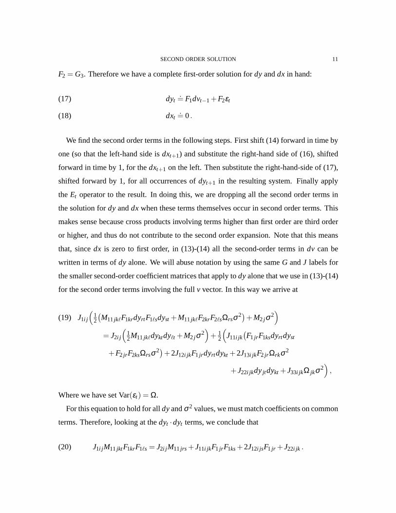
F2 = G3. Therefore we have a complete first-order solution fordyanddx in hand:

dyt.= F1dvt−1 +F2εt(17)

dxt.= 0.(18)

We find the second order terms in the following steps. First shift (14) forward in time by

one (so that the left-hand side isdxt+1) and substitute the right-hand side of (16), shifted

forward in time by 1, for thedxt+1 on the left. Then substitute the right-hand-side of (17),

shifted forward by 1, for all occurrences ofdyt+1 in the resulting system. Finally apply

theEt operator to the result. In doing this, we are dropping all the second order terms in

the solution fordy anddx when these terms themselves occur in second order terms. This

makes sense because cross products involving terms higher than first order are third order

or higher, and thus do not contribute to the second order expansion. Note that this means

that, sincedx is zero to first order, in (13)-(14) all the second-order terms indv can be

written in terms ofdy alone. We will abuse notation by using the sameG andJ labels for

the smaller second-order coefficient matrices that apply todyalone that we use in (13)-(14)

for the second order terms involving the fullv vector. In this way we arrive at

(19) J1i j

(12

(M11jk`F1krdyrt F1`sdyst +M11jk`F2krF2`sΩrsσ2)+M2 jσ2

)

= J2i j

(12M11jk`dyktdy t +M2 jσ2

)+ 1

2

(J11i jk

(F1 jr F1ksdyrt dyst

+F2 jr F2ksΩrsσ2)+2J12i jkF1 jr dyrt dykt +2J13i jkF2 jr Ωrkσ2

+J22i jkdyjt dykt +J33i jkΩ jkσ2)

,

Where we have setVar(εt) = Ω.

For this equation to hold for alldyandσ2 values, we must match coefficients on common

terms. Therefore, looking at thedyt ·dyt terms, we conclude that

(20) J1i j M11jktF1krF1`s = J2i j M11jrs +J11i jkF1 jr F1ks+2J12i jsF1 jr +J22i jk .

SECOND ORDER SOLUTION 12

This is a linear equation, and every element of it is known except forM11···. The transfor-

mations that produced the block-recursive system with ordered roots guarantee thatJ2··, an

ordinary2×2 matrix, has all its eigenvalues above the critical stability value. It is therefore

invertible, and we can multiply (20) through on the left byJ−12 , to get a system in the form

(21) AM∗F1⊗F1 = M∗+B.

In this equation,M∗ is the ordinaryns×n2s matrix obtained by stacking up the second and

third dimensions ofM11···, A = J−12 J1, andB is everything else in the equation that doesn’t

depend onM∗. If the dividing line we have specified between stable and unstable roots is

1+ δ , then our construction of the block-recursive system has guaranteed thatJ−12 J1 has

all its eigenvalues≤ 1/(1+δ ), while at the same time it is a condition on the solution that

all the eigenvalues ofF1 be< 1+ δ . To guarantee that a second-order solution exists, we

require that the largest eigenvalue ofF1⊗F1, which is the square of the largest eigenvalue

of F1, be less than the inverse of the largest eigenvalue ofA= J−12 J1. If δ = 0 this condition

is automatically satisfied. Otherwise, there is an extra condition that was not required for

finding a solution to the linear system: the smallest unstable root must exceed the square

of the largest stable root.

Assuming this condition holds, (21) has the form of a discrete Lyapunov or Sylvester

equation that is guaranteed to have a solution. Because of the special structure ofF1⊗F1,

it would be very inefficient to solve this system with standard packages (like Matlab’s

lyap.m ), but it is easy to exploit the special structure with a doubling algorithm to obtain

an efficient solution forM∗. That is, one notes that (21) implies

(22) M∗ =−∞

∑i=0

AiBFi1⊗F i

1

and defines thej ’th approximation toM∗ as

(23) M∗j =−

j−1

∑i=0

AiBFi1⊗F i

1 .

SECOND ORDER SOLUTION 13

Then the recursion, starting withM∗1 =−B,

(24) M∗2· j = M∗

j +A jM∗j F

j1 ⊗F j

1

quickly converges, unless the eigenvalue condition is extremely close to the boundary.

With M11··· in hand, it is easy to see from (19) that we can obtain a solution forM2

by matching coefficients onσ2. The only slightly demanding calculation is a required

inversion ofJ2− J1. But sinceJ−12 J1 has all its eigenvalues less than one, thisJ2− J1 is

guaranteed to be nonsingular.

The next step is to use (16) to substitute for the first-order term indxt on the right of (13)

and to use (17)-(18) to substitute for all occurrences ofdyt anddxt in second-order terms

on the right in the resulting equation. This produces an equation withdyt on the left, and

first and second-order terms indyt−1 andεt and terms inσ2 on the right. WithM11 andM2

in hand, it turns out that it is only a matter of bookkeeping to read off the values ofF12, F22,

andF3 by matching them to the collected coefficients in this equation.7

5. ANALYZING THE STATE REPRESENTATION

The gensys.m andgensys.R programs produce as output, among other things, a

first-order expansion of (9), as

(25) dwt.= F∗1 dwt−1 +F∗2 σεt .

To find a conventional state-space representation of such a system, we can form a singular

value decomposition

(26) [F∗1 F∗2 ] =[U V

]D 0

0 0

R′1 R′2

S′1 S′2

,

where[U V] and [R S] are orthonormal matrices andD is diagonal. Any state vectorzt

that has the property thatwt is determined byzt in this system will have to be of the form

7This bookkeeping is not trivial to program, but it is probably best for those who need to program it to

consult the program, rather than take up space here with the bookkeeping.

SECOND ORDER SOLUTION 14

zt = θU ′wt . The only waywt−1 affects currentwt is viaR′1wt−1. While R′1 can be the same

row rank asU , it can also be less, so that a smaller “state” vector summarizes the past than

is needed to characterize the current situation. Also, the rank ofF∗1 can be below its number

of non-zero singular values. In this case it may be possible to find azt that , after the system

has run a few periods, summarizes the past and/or characterizes the current situation yet is

of lower dimension than the rank ofD.

The programgstate.m takes as inputF∗1 andF∗2 , together with an optional candidate

matrix φ of coefficients that might form a state vector aszt = φwt . The program checks

whetherφ lies inU ’s or R′1’s row space and returnsU andR′1 for further analysis.

Once a state/co-state representation of the formvt = Ψwt has been settled on, whereΨ is

non-singular and thev = (y′ x′)′ vector is partitioned into state and costate, it is straightfor-

ward to convert a first or second-order approximate solution from one co-ordinate system

into the another.

6. THE LOCAL ACCURACY OF THE APPROXIMATION

Once we have a second-order accurate approximation to the dynamics, in the form (15)-

(16), we can make a claim to local accuracy of the following form:

(27) dvt+1 = F(dvt ,σεt+1,σ)+op(‖dvt ,σ‖2) ,

whereop means “order in probability” andF is the second-order approximation to the

dynamics. That is, the error in the approximation is claimed to converge in probability to

zero, at a more rapid rate than‖dvt ,σ‖2, when‖dvt ,σ‖2 goes to zero. This rate is the

weakest kind of claim that can be made for a Taylor expansion. If we are willing to claim

that third derivatives exist at the deterministic steady state, then we can replace the error

term withOp(‖dvt ,σ‖3). This claim does not depend on strict boundedness of the support

of the distribution ofεt , because we are only claiming our local accuracy with a certain

(high) probability. Whatever the distribution ofεt , σεt converges in probability to zero as

σ → 0, allowing us to make this claim. Of course this is all dependent on the underlying

assumption that the original nonlinear model has dynamics differentiable of sufficiently

SECOND ORDER SOLUTION 15

high order inσ in the neighborhood of deterministic steady state, and on the existence and

continuity of the expectations that occur in the statement of the model.

This one-step-ahead “local accuracy in probability” claim obviously can be extended

to a corresponding claim to accuracyn-steps-ahead for any finiten. We have made no

appeal to stationarity of the system in making these claims. Of course the size of then for

which accuracy remains good at a given level ofσ will in general be smaller for systems

that are not stationary. But the qualitative nature of the accuracy claim is no different for

non-stationary systems.

This type of finite-time-span, accuracy-in-probability claim is exactly what is appropriate

for purposes of fitting a model to data — which always cover a finite time span — or for

purposes of simulating the model from given initial conditions over a finite span of time. It

is also exactly appropriate for the correct calculation of expected welfare, when welfare is

constructed as a discounted sum of period utilities. The discounting means that accuracy

of the approximation is unimportant after some time horizon in the future.

It goes without saying that no theoretical result about local or asymptotic global accu-

racy for approximate solutions can prove that in a particular model, with particular shock

variances, one method or another is more accurate than another or accurate enough for

some specific purpose. The emphasis byJin and Judd(2002) on checking model validity is

therefore appropriate. There is no uniquely best measure of solution accuracy, but by now

a variety of stringent checks have been proposed. The methods that have been applied most

widely (but not widely enough) are based on evaluating the conditional expectation in (3) at

a collection of values of the lagged state vector. There are important practical questions as

to how to select the collection of state vector values at which one evaluates the expectation

and as to what metric to use in measuring the vector of deviations from the theoretical zero

values for these expectations. Jin and Judd suggest deterministically fixing a collection

of state variable values and a set of “relative error” metrics for the expectational errors,

based on economic interpretation of the model being solved.den Haan and Marcet(1994)

suggest another approach, in which the state variable values are generated stochastically

SECOND ORDER SOLUTION 16

via simulation and the metric for evaluation of expectational errors is based on statistical

detectability of the errors in a sample of relevant length. Each of these approaches has

pitfalls, but is worth consideration.

Though there is no widely understood alternative to this “Euler equation residual” family

of accuracy checks at this point, there is probably room for further work in this area. For

many purposes, the most relevant measure of accuracy is the accuracy of the solution’s

approximation to the mapping fromwt−1, εt , andσ to wt corresponding to (9). This is not

measured directly by the size of the Euler equation errors, but no more direct measure of

the accuracy of this mapping is at this point commonly computed. The usual approaches

to assessing numerical accuracy in nonlinear models could be applied here. For example,

one could sample from solutions that are close to equivalent by the Euler equation accuracy

criterion and describe the degree to which the solution function varies while Euler equation

error stays within the convergence criteria.

7. FORECASTING AND SIMULATION

Forecastss steps ahead,Et [dwt+s] andVart [dwt+s] are the building blocks for the calcu-

lation of impulse response functions as well as welfare.

We build the forecasts from the second-order accurate dynamic model given by (15)-

(16), modified here to reflect our assumption that the initial conditions satisfy the equations

of the model and that thereforedxt−1 = 0 to first order. We abuse notation by using the

sameF ’s here, for the pieces of the originalF matrices corresponding tody’s, as we did

for the originalF matrices in (15)-(16) that corresponded to the fulldv= [dy,dx] vector.

dyt.= F1 jdyj,t−1 +F2 jσε j,t +F3σ2

+ 12F11jkdyj,t−1dyk,t−1 +F12jkσdyj,t−1εk,t + 1

2F22jkσ2ε j,tεk,t(28)

dxt.= 1

2M11jkdyj,tdyk,t +M2σ2(29)

We would then like to calculate, to second order accuracy,Et [dyt+s] andVart [yt+s].

SECOND ORDER SOLUTION 17

To begin with, note that, since the conditional mean ofdyt+s is of second order, the vari-

ance termsΣs≡ Vart (yt+s) are correct to second order accuracy when computed from the

first-order terms in the expansion (28) alone and that, to second-order accuracy,Vart (xt+s)=

0 sincedxt itself is of second order.

For s= 1, it is easy to see from (28)-(29) that we have

dyt+1 = Et [dyt+1].= F1 jdyj,t +F3σ2

+ 12F11jkdyjt dykt +

σ2

2F22jkΩ jk

(30)

dxt+1 = Et [dxt+1].= 1

2M11jk(dy j,t+1dyk,t+1 + Σ1 jk

)+M2σ2 .(31)

The expression in (31) for determiningEt [dxt+1] from the conditional mean and variance of

dyt+1 works equally well for determiningEt [dxt+s] from the conditional mean and variance

of dyt+s for s> 1. The straightforward approach to determiningdyt+s anddxt+s is to apply

(30) recursively, computingdyt+s from dyt+s−1 and Σk−1, etc. This procedure is in fact

second-order accurate, but it introduces higher order terms into the expansion. For example,

sincedyt+1 contains quadratic terms indyt , and (30) makesdyt+2 quadratic indyt+1, in a

simple recursive computationdyt+2 becomes quartic indyt . These extra high-order terms

do not in general increase accuracy of the approximation, as they do not correspond to

higher order coefficients in a Taylor series expansion of the true dynamic system, and in

practice often lead to explosive time paths fordyt+s.

To see what goes wrong, consider the simple univariate model

yt = ρyt−1 +αy2t−1 + εt ,

where|ρ |< 1 andα > 0. Though this model is locally stable about its unique deterministic

steady state ofy = 0, it has a second steady-state, at(1− ρ)/α. If y exceeds the other

steady state, it will tend to diverge. This is likely to be a generic problem with quadratic

expansions — they will have extra steady states not present in the original model, and some

of these steady states are likely to mark transitions to unstable behavior.

SECOND ORDER SOLUTION 18

Since the unique local dynamics are stable in a neighborhood of the steady state, it will be

desirable to choose amongst the second order accurate expansions one that implies stability.

Deriving sufficient conditions on the support ofεt to guarantee non explosiveness under the

iterative scheme (30)-(31) is in general a non-trivial task and therefore it is useful to have

available an algorithm which generates non-explosive forecasts and simulations without

imposing explicit conditions on the support ofεt . The mere fact that the generated forecasts

are stable of course does not imply superior accuracy in general, especially when shocks

are not bounded. However, stationarity will in general imply that, for a given neighborhood

U of the steady state and a given time horizonT, we can restrictσ in such a way as to

make the probability of leavingU in time T arbitrarily small.

Obtaining a stable solution based on (30) can be achieved by pruning out the extraneous

high-order terms in each iteration by computing the projections of the second order terms

based on afirst-orderexpansion,dyt+1 of Et [dyt+1], as follows:

dyt+s.= F1 jdy j,t+s−1 +F3σ2

+ 12F11jk

(dy j,t+s−1dyk,t+s−1 + Σk−1, jk

)+ σ2

2 F22jkΩ jk

(32)

dxt+s.= 1

2M11jk(dy j,t+sdyk,t+s+ Σs, jk

)+M2σ2(33)

dyt+s.= F1 jdy j,t+s−1(34)

Σi j ,s = σ2F2ikΩk`F2 j` +F1ikΣk`,s−1F1 j` .(35)

Using these equations recursively results in adyt+s series which, by construction, is

quadratic indyt for all s. Furthermore, when the eigenvalues ofF1 are less than one in

absolute value, the first order accurate solutiondyt+s is stable and hence so is the squared

process(dy j,t+sdyk,t+s

). It follows that dyt must be stable as well.8 Note that theF12

component of the second order expansion — the coefficients of the interactions between

dyt−1 andεt — do not enter this recursion at all.

8The same matrix eigenvalue conditions are at issue here as in section4’s discussion of existence of the

solution to (21)

SECOND ORDER SOLUTION 19

The same issues arise if the aim is to generate simulated time paths, rather than simply

conditional expectations and variances of future variables. For this purpose, we can intro-

duce the notationdy(1)t+s anddy(2)

t+s for first and second order accurate simulated time paths,

respectively. A recursive, non-explosive, “pruned” simulation scheme is then given by

dy(2)t+s

.= F1· jdy(2)j,t+s−1 +F2· jσε j,t+s+F3σ2

+ 12F11· jkdy(1)

j,t+s−1dy(1)k,t+s−1 +σF12· jky(1)

j,t+s−1εk,t+s+ σ2

2 F22· jkε j,t+sεk,t+s

(36)

dx(2)t+s

.= 12M11· jkdy(1)

j,t+sdy(1)k,t+s+M2σ2(37)

dy(1)t+s

.= F1· jdy(1)j,t+s−1 +F2· jσε j,t+s ,(38)

where theF12 terms that could be ignored in forming conditional expectations have neces-

sarily returned for generation of accurate simulations. By preventing buildup of spurious

higher-order terms, we make stability of the simulation over a long time path more likely,

while at the same time preserving second-order accuracy of the mapping from initial vari-

able valuesyt ,xt , shocksεt+1, . . . ,εt+s, andσ to the simulated valuesy(2)t+1, . . . ,y

(2)t+s.

It can help in understanding these recursions to append the vectordy(1)⊗dy(1) to dy(2)

and use matrix notation:

(39)

dy(2)

t+1

(dy(1)t+1⊗dy(1)

t+1)

= Θ1

dy(2)

t

(dy(1)t ⊗dy(1)

t )

+Θ2σ2 +ξt+1

with

Θ1 =

F1

12(F∗11)

0 (F1⊗F1)

(40)

Θ2 =

F3 + 1

2F22· jkΩ jk

(F2⊗F2)vec(Ω)

(41)

ξt =

σεt +σF23· jkεk,tdy(1)

j,t−1 + σ2

2 F33· jk(ε jt εkt−Ω jk)

σ2(εt ⊗ εt − (F2⊗F2)vec(Ω)

)

.(42)

TheF∗11 in the definition ofΘ1 (40) is a matrix with number of rows equal to the length of

y and with the second and third dimensions of the array vectorized into a row vector — so

SECOND ORDER SOLUTION 20

it is an ns×n2s matrix. Note thatΘ1 is upper block triangular and is stable exactly when

the eigenvalues ofF1 are less than one in absolute value. Note also that, to second order

accuracy,

Var(ξt) =

σ2Ω 0

0 0

.

Calculations of conditional and unconditional first and second moments can therefore be

carried out using (39) as if it were an ordinary first order VAR. This can be an aid to

understanding, or to computation in small models, though for larger systems it is likely to

be important for computational efficiency to take account of the special structure of theΘ j

matrices in (39).

Finite-time-span, accuracy-in-probability claims will not justify estimating unconditional

expectations of any functions of variables in the model via simulation. To make the effects

of initial conditions die away, such simulations must cover long spans of time. If the

second-order approximation is non-stationary, expectations calculated from simulations of

it will of course not converge. If the true nonlinear model is non-stationary, then the true

unconditional expectations will in general not exist, even though it is possible that the local

second-order approximation is stationary, so again in this case it will not be possible to

estimate unconditional expectations from simulated paths.

When both the true nonlinear model and the second order approximate model are station-

ary and ergodic, and the true unconditional expectation in question is a twice-differentiable

function ofσ in the neighborhood ofσ = 0, then it is possible to estimate the expectation

from long simulations of the approximate model, with the estimates accurate locally inσ

in the usual sense. This is true even though it may be (e.g. because of unbounded support

of εt) that with probability one the path of the model repeatedly enters regions where the

local approximation is inaccurate. This is possible because asσ → 0 the fraction of time

spent in these regions goes to zero, for both the true and the approximate model.

SECOND ORDER SOLUTION 21

However it will most often be preferable to estimate an expectation by using the second-

order approximation analytically, expanding the function whose expectation is being taken

as a Taylor series by the methods described in this section.

8. WELFARE

One can easily produce cases where the second-order approximation is necessary to get

an accurate evaluation of certain aspects of the model. Utility-based welfare calculation is

one case. For example, calculating welfare effects of various monetary and fiscal policies

or welfare effects of changes in economic environment such as financial market structure

should include second-order or even higher-order terms in order to get an accurate mea-

sure.Kim and Kim (2003a) present an example of how inaccurate the linearized solution

can be in calculating welfare using a two-country model. Using the linearized solution,

welfare of autarky can appear to be higher than that of the complete markets, solely because

of the inaccuracy of the linearization method. Another application in which second-order

approximation is important is examination of asset price behavior in DSGE’s. Linearized

solutions will imply equal expected returns on all assets. Second order solutions will gen-

erate correct risk premia, though generally to analyze time variation in risk premia will

require higher than second-order accuracy.

Equation (39) makes it relatively straightforward to see how to carry out a second-order

accurate welfare calculation. Welfare is defined as a discounted sum of expected utility.

Let the period utility function be given byu : Rns → R.9 Then the utility conditional on an

9Of course often in growth models utility is a function of consumption, which is not a conventional state

variable. To use the formulation we develop here, then, consumption (anx variable) has to be replaced by the

corresponding component ofh(y,σ). Also, because we work entirely in terms ofy, we are not covering the

case where the initial distribution ofw does not lie on the saddle path. The methods we describe here can be

expanded to cover this case and to allowx to enteru, at the cost of some increase in the burden of notation.

SECOND ORDER SOLUTION 22

initial distribution ofy0 with mean and variance(µ ,Σ) is

U(µ,Σ) = E0

[∞

∑t=0

β tu(yt)

]≈

u(y)1−β

+E0

[∞

∑t=0

β t(∇u(y)dy(2)t + 1

2 vec(∇2u(y))′(dy(1)t ⊗dy(1)

t ))]⇒

(43)

U(µ,Σ) =u(y)1−β

+[∇u(y) 1

2 vec(∇2u(y))′]

· [I −βΘ1]−1

µ

vec(Σ+ µµ ′)

+β (1−β )−1Θ2σ2

(44)

If we are interested only in unconditional expectedu, we can arrive at the correct formula

by multiplying (44) through by1−β and taking the limit asβ → 1, giving us

(45) E[u(yt)] = u(y)+[∇u(y) 1

2 vec(∇2u(y))′](I −Θ1)−1Θ2σ2 .

Note that in (44) we make no use, explicitly or implicitly, ofF12. Also note that though

the matrixI −βΘ1 appears in the formula inverted, the utility calculation only requires

[∇u(y) 1

2 vec(∇2u(y))′]· (I −βΘ1)−1 ,

whose computation is only an equation-solving problem, not a full inversion;10 further-

more, this part of the computation does not need to be repeated asµ and Σ are varied.

Finally, note that (45) uses only(I −Θ1)−1Θ2, regardless of the form ofu. This is again

an equation-solving problem. So if we are interested only in unconditional expectations,

even in unconditional expectations of many different functionsu, the computation of a

full second-order correction may be much simpler than calculation of the full second-order

expansion of the dynamics.

10Though for ann×n matrix A both solvingAx= b for x and computingA−1 areO(n3) operations, the

latter is substantially more time consuming. In Matlab inversion takes roughly twice the time.

SECOND ORDER SOLUTION 23

It is these simplifications, applied to particular models, that are the insights provided by

the papers that have put forward “bias-correction” methods for making second-order accu-

rate expected welfare computations in DSGE models (Kim and Kim, 2003a; Sutherland,

2002).

We should note that there is a situation in which second-order accurate evaluations of

welfare can avoid entirely the need for a second-order expansion of the model solution.

If ∇u(y) = 0, as would be true if the deterministic steady-state setsy to the value that

maximizesu(y), then only the lower blocks ofΘ1 and Θ2 enter the solution, as can be

seen from (44) or (45). As can be seen from (40) and (42), these blocks containF1 and

F2 only, not any terms from the second-order solution. Of course in most problems with

discounting, even an optimal solution will not maximize static welfareu(y) in the steady

state, so this result will not apply. Also, even where the solution has been computed to

maximize static period welfareu, the result depends on having a second order expansion of

u in terms of the state vectory. When the problem has been formulated (as in usual growth

models) with a non-state variable (e.g. consumption) appearing in the utility function, the

second-order expansion of the utility function in terms ofy may require use of the second-

order solution forx as a function ofy.11

8.1. Conditional vs. Unconditional welfare. From the discussion in the preceding sec-

tion it is apparent that evaluating expected welfare based on unconditionalE[u(y)] is a

more straightforward task than evaluating the conditional expectation of discounted ex-

pected utility at a given date.12 It is therefore not surprising that many existing papers have

11Rotemberg and Woodford(1997) is an example of a context where use of the first-order solution for

welfare analysis is justified by special regularity conditions. The paper evaluated welfare using unconditional

expectation of period utility. Regularity conditions required to justify use of the first-order solution in the

paper’s model include an assumption that some other policy change perfectly offsets second-order effects of

monetary policy on the mean level of output and an assumption that monetary policy is the only source of

inefficient fluctuations in prices.12Woodford(2002) discusses the differences between unconditional and conditional welfare in calculating

welfare effects of monetary policies.

SECOND ORDER SOLUTION 24

used unconditional welfare for evaluating policies. Examples includeClarida, Galı, and

Gertler(1999), Rotemberg and Woodford(1997, 1999), Sutherland(2002) andKollmann

(2002).

There are strong objections in principle to use of the unconditional welfare criterion. We

know that it takes time for one steady state to reach another steady state and unconditional

welfare neglects the welfare effects during the transitional period. It is therefore generally

not in fact optimal, in problems with discounting, to use policies that maximize the uncon-

ditional expectation of one-period welfare. This is not a new point — it is the same point as

the non-optimality of driving the rate of return to zero in a growth model — and it has been

recognized in the DSGE literature in, e.g,Kim and Kim(2003b), andWoodford(2002).

Because unconditional welfare can often be computed easily, using the “bias correc-

tion” shortcut, it is important to note that using unconditional welfare can give nonsen-

sical results.Kim and Kim (2003a) construct a two-country DSGE model and compute

risk-sharing gains from autarky to the complete-markets economy using a second-order

approximation method. Welfare is defined as conditional welfare and the results show that

there are positive welfare gains from autarky to the complete-markets economy. But the

unconditional welfare measure can for certain parameter values produce the paradoxical

result that autarky generates a higher level of welfare than the complete markets.

The use of conditional welfare does not imply that results necessarily are tied to some

particular initial state. One can condition on a distribution of values for the initial state.

The critical point is that when comparing two policies or equilibria one should use the same

distribution for the initial state for each. When there is no time-inconsistency problem the

optimal policy will have the property that no matter what initial distribution is specified for

the state, it will produce a higher conditional expectation of welfare than any other policy.

However, when comparing a collection of policies that are not optimal, one may find that

rankings of policies vary with the assumed distribution of the initial state.

When there is a time-inconsistency problem, the optimal policy generally depends on the

initial conditions, even if we restrict attention to policy rules that are a fixed mapping from

SECOND ORDER SOLUTION 25

state to actions. Using a conditional expectation as the welfare measure does not avoid

this problem. One attempt to get around this issue is the suggestion in, e.g.,Giannoni and

Woodford(2002) that policy should follow the rule that would prevail under commitment

in the limit as the initial conditions recede into the past. This “timeless perspective” policy

can be implemented by treating the Lagrange multipliers on private sector Euler equations

as “states”, and then maximizing conditional expected discounted utility.13

9. CONCLUSION

Use of perturbation methods to improve analysis of DSGE models is still in its early

stages. Programs that automate computations for models higher than second order are

just beginning to emerge. Methods of dealing with the kinds of singularities that show

up in economic models — for example the indeterminacy of asset allocations in standard

portfolio problems when variances are zero — are still not widely understood. And we have

only begun to get a feel for where these methods are useful and what their limitations are.

Real progress is being made, however, in an atmosphere that is both competitive enough

to be stimulating and cooperative enough that researchers located around the world are

benefiting from each others’ insights.

13Note that though the timeless perspective policy is a useful benchmark, it cannot resolve the fundamen-

tal problem of time inconsistency. A policy-maker who can make believable commitments will not want to

choose the timeless-perspective solution, while one that cannot make believable commitments cannot imple-

ment the timeless-perspective solution.

SECOND ORDER SOLUTION 26

REFERENCES

ANDERSON, G., AND A. L EVIN (2002): “A user-friendly, computationally-efficient al-

gorithm for obtaining higher-order approximations of non-linear rational expectations

models,” Discussion paper, Board of Governors of the Federal Reseerve.

BERGIN, P. R.,AND I. TCHAKAROV (2002): “Does Exchange Rate Risk Matter for Wel-

fare? A Quantitative Investigation,” Discussion paper, University of California at Davis,

http://www.econ.ucdavis.edu/faculty/bergin/ .

CLARIDA , R., J. GAL I , AND M. GERTLER (1999): “The science of monetary policy: A

new Keynesian perspective,”Journal of Economic Literature, 37, 1661–1707.

COLLARD , F., AND M. JUILLARD (2000): “Perturbation Methods for Rational Ex-

pectations Models,” Discussion paper, CEPREMAP, Paris,fabrice.collard@

cepremap.cnrs.fr .

DEN HAAN , W. J., AND A. M ARCET (1994): “Accuracy in Simulations,”The Review of

Economic Studies, 61(1), 3–17.

GASPAR, J.,AND K. L. JUDD (1997): “Solving large-scale rational expectations models,”

Macroeconomic Dynamics, 1, 44–75.

GIANNONI , M. P.,AND M. WOODFORD(2002): “Optimal Interest-Rate Rules: I. General

Theory,” Discussion paper, Columbia University and Princeton University,http://

www.princeton.edu/˜woodford .

JIN , H., AND K. L. JUDD (2002): “Perturbation Methods for General Dynamic Stochastic

Models,” Discussion paper, Stanford University,judd@hoover.stanford.edu .

JUDD, K. L. (1998):Numerical Methods in Economics. MIT Press, Cambridge, Mass.

K IM , J., AND S. KIM (2003a): “Spurious Welfare Reversals in International Business

Cycle Models,”Journal of International Economics, 60, 471–500.

(2003b): “Welfare Effects of Tax Policy in Open Economies: Stabilization and

Cooperation,” Discussion paper, University of Virginia and Tufts University,http:

//www.tufts.edu/˜skim20 .

SECOND ORDER SOLUTION 27

K ING, R. G., AND M. WATSON (1998): “The Solution of Singular Linear Difference

Systems Under Rational Expectations,”International Economic Review, 39(4), 1015–

1026.

KLEIN , P.(2000): “Using the generalized Schur form to solve a multivariate linear rational

expectations model,”Journal of Economic Dynamics and Control, 24(10), 1405–1423.

KOLLMANN , R. (2002): “Monetary Policy Rules in the Open Economy:Effects on Wel-

fare and Business Cycles,”Journal of Monetary Economics, 49, 989–1015,http:

//www1.wiwi.uni-bonn.de/users/rkollmann/www/ .

ROTEMBERG, J. J.,AND M. WOODFORD(1997): “An Optimization-Based Econometric

Framework for the Evaluation of Monetary Policy,”NBER Macro Annual, 12, 297–345.

(1999): “Interest rate rules in an estimated sticky-price model,” inMonetary Policy

Rules, ed. by J. B. Taylor. University of Chicago Press, Chicago.

SCHMITT-GROHE, S., AND M. URIBE (2002): “Solving dynamic general equilibrium

models using a second-order approximation to the policy function,” Discussion paper,

Rutgers University and University of Pennsylvania.

SIMS, C. A. (2001): “Solving Linear Rational Expectations Models,”Computational Eco-

nomics, 20(1-2), 1–20,http://www.princeton.edu/˜sims/ .

SUTHERLAND, A. (2002): “A simple second-order solution method for dynamic gen-

eral equilibrium models,” Discussion paper, University of St. Andrews,http://www.

st-andrews.ac.uk/˜ajs10/home.html .

WOODFORD, M. (2002): “Inflation Stabilization and Welfare,”Contributions to Macroe-

conomics, 2(1), Article 1.

FEDERAL RESERVEBOARD, TUFTS UNIVERSITY, NORTHWESTERNUNIVERSITY, PRINCETON UNI-

VERSITY

E-mail address: sims@princeton.edu

WORKING PAPER SERIES 2005 http://ase.tufts.edu/econ/papers/papers.html

2005-01 EGGLESTON, Karen, Keqin RAO and Jian WANG; “From Plan

to Market in the Health Sector? China's Experience.”

2005-02 SHIMSHACK Jay; “Are Mercury Advisories Effective?

Information, Education, and Fish Consumption.”

2005-03 KIM, Henry and Jinill KIM; “Welfare Effects of Tax Policy in

Open Economies: Stabilization and Cooperation.”

2005-04 KIM, Henry, Jinill KIM and Robert KOLLMANN; “Applying

Perturbation Methods to Incomplete Market Models with

Exogenous Borrowing Constraints.”

2005-05 KIM, Henry, Jinill KIM, Ernst SCHAUMBURG and Christopher

A. SIMS; “Calculating and Using Second Order Accurate

Solutions of Discrete Time Dynamic Equilibrium Models.”

2005-06 KIM, Henry, Soyoung KIM and Yunjong WANG; “International

Capital Flows and Boom-Bust Cycles in the Asia Pacific Region.”

2005-07 KIM, Henry, Soyoung KIM and Yunjong WANG; “Fear of

Floating in East Asia.”

2005-08 SCHMIDHEINY, Kurt; “How Fiscal Decentralization Flattens

Progressive Taxes.”

2005-09 SCHMIDHEINY, Kurt; “Segregation from Local Income Taxation

When Households Differ in Both Preferences and Incomes.”

2005-10 DURLAUF, Steven N., Andros KOURTELLOS, and Chih Ming

TAN; “How Robust Are the Linkages between Religiosity and

Economic Growth?”

2005-11 KEELY, Louise C. and Chih Ming TAN; “Understanding

Preferences For Income Redistribution.”

2005-12 TAN, Chih Ming; “No One True Path: Uncovering the Interplay

between Geography, Institutions, and Fractionalization in

Economic Development.”

2005-13 IOANNIDES, Yannis and Esteban ROSSI-HANSBERG; “Urban

Growth.”

2005-14 PATERSON, Robert W. and Jeffrey E. ZABEL; “The Effects of

Critical Habitat Designation on Housing Supply: An Analysis of

California Housing Construction Activity.”

2005-15 KEELY, Louise C. and Chih Ming TAN; “Understanding

Divergent Views on Redistribution Policy in the United States.”

2005-16 DOWNES, Tom and Shane GREENSTEIN; “Understanding Why

Universal Service Obligations May Be Unnecessary: The Private

Development of Local Internet Access Markets.”

2005-17 CALVO-ARMENGOL, Antoni and Yannis M. IOANNIDES;

“Social Networks in Labor Markets.”

2005-18 IOANNIDES, Yannis M.; “Random Graphs and Social Networks:

An Economics Perspective.”

2005-19 METCALF, Gilbert E.; “Tax Reform and Environmental

Taxation.”

2005-20 DURLAUF, Steven N., Andros KOURTELLOS, and Chih Ming

TAN; “Empirics of Growth and Development.”

2005-21 IOANNIDES, Yannis M. and Adriaan R. SOETEVENT; “Social

Networking and Individual Outcomes Beyond the Mean Field

Case.”

2005-22 CHISHOLM, Darlene and George NORMAN; “When to Exit a

Product: Evidence from the U.S. Motion-Pictures Exhibition

Market.”

2005-23 CHISHOLM, Darlene C., Margaret S. McMILLAN and George

NORMAN; “Product Differentiation and Film Programming

Choice: Do First-Run Movie Theatres Show the Same Films?”

2005-24 METCALF, Gilbert E. and Jongsang PARK; “A Comment on the

Role of Prices for Excludable Public Goods.”