Embed Size (px)
Citation preview

From the Cradle to the Grave? The Effect of Birth Weight on Adult Outcomes of Children*
PRELIMINARY AND INCOMPLETE
by
Sandra E. Black Department of Economics UCLA, IZA and NBER [email protected]
Paul J. Devereux
Department of Economics University College Dublin and IZA
Kjell G. Salvanes Department of Economics
Norwegian School of Economics, Statistics Norway and IZA [email protected]
September 2005
* Black and Devereux gratefully acknowledge financial support from the National Science Foundation and the California Center for Population Research.

1
Abstract
Lower birth weight babies have worse outcomes, both short-run in terms of one-year mortality rates and longer run in terms of educational attainment and earnings. However, recent research has called into question whether birth weight itself is important or whether it simply reflects other hard-to-measure characteristics. By applying within twin techniques using a unique dataset from Norway, we examine both the short-run and long-run outcomes for the same cohorts. In addition, because we observe a large amount of information on both parents and children, we look at whether positive parental characteristics are able to mitigate the effects of low birth weight on children’s outcomes. We find that birth weight does matter; very small short-run effects can be misleading because longer-run effects on outcomes such as height, IQ, earnings, and education are significant. There is little evidence that parental resources are able to mitigate the negative effects of low birth weight.

2
1. Introduction
Lower birth weight babies have worse outcomes, both short-run in terms of one-
year mortality rates and longer run in terms of educational attainment and earnings.
However, recent research has called into question whether birth weight itself is important
or whether it simply reflects other hard-to-measure characteristics. If birth weight does
not matter in the long-run, can government policies targeting the welfare of children
through improved pre-natal care actually work?
Governments have assumed that birth weight is important and have implemented
policies to improve the health of pregnant women in the hope that this will improve the
outcomes of their babies; consider, for example, the Women, Infants, and Children
Program (WIC), a federally funded program that provides nutrition counseling and
supplemental food for pregnant women, new mothers, infants and children under age five
in order to prevent children's health problems and improve their long-term health, growth
and development. A key presumption underlying this type of policy is that, by affecting
children’s birth weight through improved nutritional intake in utero, it will in turn affect
the later health and ultimate success of the children. But is this presumption valid? That
is, does birth weight as a proxy for health at birth have a causal effect on children’s
outcomes? While there is much evidence that low birth weight children experience
greater health difficulties as infants, there is little evidence about whether being low birth
weight (LBW) has a causal effect on later outcomes.
Despite this, researchers often use birth weight as an outcome measure with the
belief that it does have a longer-run causal relationship.1 Birth weight is very commonly
1 Barker (1995) finds evidence that fetal undernutrition is related to coronary heart disease later in life. Other recent work in the Norwegian medical literature also finds a positive relationship between birth

3
used as the outcome variable of interest in studies of the effects on infant welfare of
policy interventions such as welfare reform, health insurance, and food stamps (for
example, Currie and Gruber, 1996). Likewise, birth weight is often used as an outcome
variable in studies of the effects of inputs to the infant health production function and
analyses of the impact of maternal behavior on infant health (for example, Currie and
Moretti, 2003 show that increased maternal education leads to a lesser incidence of
LBW). Obviously, the degree to which LBW has true causal effects on later outcomes is
critical to the interpretation of the results from this literature.
The principal difficulty in determining the effects of LBW on later outcomes
arises because LBW is likely correlated with a range of socio-economic and genetic
characteristics of families and their children. For example, LBW infants are more likely
to be born to poor families; as a result, it is difficult to disentangle the effects of birth
weight from that of family income. Our approach is to use twin comparisons to
distinguish between LBW effects and other socio-economic and genetic effects.
Using a unique dataset on the population of births in Norway matched with later
outcomes along with extensive information on parents, we are able to examine both the
short- and long-run effects of birth weight for the same cohort of individuals. We
advance the recent literature by using twin fixed effects on a large sample of individuals
and looking at both short- and long-run outcomes. The current literature has examined
the effects of low birth weight using within family and, most recently, within twin
estimates of the effect of birth weight on both early outcomes (Almond et al 2005) and
later outcomes (Berhman and Rosenzweig 2004) separately. Almond et al suggest that
weight on adult outcomes. (Eide et al. (2005) and Grjibovski et al. (2005)) In addition, there is some research in the medical literature examining whether the negative effects of low-birth weight may be self-correcting over time. See Ment et al (2003)

4
cross-sectional estimates of the effects of birth weight greatly overstate the true effects
when they apply twin fixed effects and look at early outcomes such as one year mortality
rates; in contrast, Behrman and Rosenzweig find exactly the opposite (the within twin
estimates are much larger than OLS estimates) when they look at longer run outcomes
such as education, height, and wages. No dataset to date has been able to study both
short-run and long-run outcomes for the same cohorts. This paper fills this void in the
literature.
We find that birth weight does matter. Consistent with earlier findings, we find
that it has only a small effect on short-run outcomes such as one-year infant mortality;
however, these short-run studies can be misleading, as we find that, despite small short-
run effects on infant mortality, birth weight has a significant effect on longer-run
outcomes such as height, IQ at age 18, earnings and education.
Given these findings, an important issue is whether the effects of low-birth weight
can be offset by family resources. Can family income mitigate any negative effects of
low-birth weight? We study how the effects of birth weight differ amongst children born
into families of different socio-economic status and find some evidence that family
income can offset the negative effects of lower birth weight.
The paper unfolds as follows. Section 2 reviews the relevant literature, Sections 3
and 4 discuss our methodology and data. Section 5 presents our results and robustness

5
checks, and Section 6 focuses on the ability of parents to offset the negative effects of
low birth weight. Section 7 addresses issues of generalizability, and Section 8 concludes.
2. Relevant Literature
There is a long history of research across disciplines relating low birth weight to
poor health, cognitive deficits, and behavioral problems among young children, as well as
some evidence that this relationship persists for longer-term outcomes. For example,
Currie and Hyson (1998) find a relationship between birth weight and educational
attainment, employment, wages, and health status at age 23 and age 33. More recently,
Case et al. (2004) show that, controlling for family background measures, children with
low birth weight and poorer childhood health indicators have significantly lower
educational attainment, poorer health, and lower SES as adults. However, it is possible
that there is no causal relationship underlying these correlations, as low birth weight may
be correlated with many difficult-to-measure socio-economic background and genetic
variables.3
To ascertain the causal effect of LBW on child outcomes, one requires variation
in birth weight that is unrelated to genetic and socio-economic characteristics. Since
researchers cannot randomly assign birth weights to children, the few papers that have
not used OLS instead use sibling or twin fixed effects models.
3 There is also much research in the medical literature investigating the effects of low birth weight on children’s outcomes. Unfortunately, similar to the economics literature, they have limited data on longer-run outcomes and small sample sizes, rendering any within-family analysis impossible. For example, Hack et al (1994) finds an effect of very low birth weights on school age outcomes using 68 treatment children using across family comparisons and Hack et al (2002) compare 242 very low birth weight young adults to 233 normal birth weight controls and find that the educational disadvantage associated with very low birth weight persists into early adulthood.

6
The sibling fixed effects approach involves comparing the outcomes of siblings
who differ in birth weight. This approach conditions out any characteristic that is family-
specific and unchanging over time but is not robust to time-varying unobserved
characteristics, such as the quality of pre-natal care received by the mother, which may
vary across pregnancies. Also, siblings share only about 50% of their genetic material so
there may be genetic differences across siblings that are correlated with birth weight.4
Most recently, the literature has moved to within twin variation to identify the
effects of birth weight on children’s outcomes. Both Conley, Strully, and Bennett (2005)
and Almond, Chay, and Lee (2005) use U.S. data to identify the effects of birth weight on
short run health outcomes, including mortality. Almond et al. conclude that the effects of
low birth weight are substantially smaller than originally thought; Conley et al come to a
similar conclusion although argue that, though one overestimates the effect of low birth
weight on neonatal mortality (within 28 days of birth), there is still a significant and large
effect on the probability of infant mortality at one year. However, neither of these studies
is able to look beyond short-run health outcomes.
Behrman and Rosenzweig (2004) use a subset of the Minnesota Twin Registry to
do fixed effects using female monozygotic twins. 5 They find evidence that the heavier
4 Conley and Bennett (2000) take a sibling fixed effects approach using data from the Panel Study of Income Dynamics (PSID). They find a negative association between LBW and timely high school graduation. Currie and Moretti (2005) use sibling comparisons to investigate the effects of birth weight on the birth weight of the child’s future children. They also show that among mothers that were siblings, the women with the lower birth weight resided in a lower income zip code on average when she gave birth to her own child years later. 5 One concern with monozygotic twins is that the results may not be generalizable. Conley, Strully, and Bennett (2005) point out that, unlike siblings and fraternal twins, monozygotic twins have the same “ideal” weight. Then, if genetic differences in birth weight have lesser consequences than differences due to prenatal competition, then generalizing from identical twins may lead to an overstatement of the effects of birth weight. Conley and Bennett also argue that because monozygotic twins frequently share a placenta, a smaller genetically identical twin may be more nutritionally deprived than a singleton birth or fraternal twin of the same weight. However, given that policy focuses on the effect of improving birth weight through improved pre-natal nutrition, this might be the appropriate comparison.

7
twin goes on to be taller, have greater schooling attainment, and to have a higher wage. In
contrast, they find no evidence of effects on the birth weights of future children.
However, the sample sizes are small (804 cases) and because of the numerous surveys
required, there is substantial attrition and item non-response, that may not be random.
Our study differs from Behrman and Rosenzweig in that we study both men and women,
use larger nationally representative samples from administrative data, and use outcome
variables that are not self-reported.
3. Conceptual Framework
Let
ijkjkjkijkijk fxbwy εγβα ++++= ' (1)
where subscript i refers to the child, j refers to the mother, and k refers to birth. ijky is
then the outcome of child j born to mother i in birth k, ijkbw is birth weight, jkx is a
vector of mother- and birth-specific variables (for example, mother’s education, the year
of birth), jkf refers to unobservables that are mother- and birth-specific (for example, the
quality of pre-natal care, genetic factors), and ijkε is an idiosyncratic error term assumed
independent of all other terms in the equation.6
The parameter of interest is β -- the effect of birth weight on the outcome
variable holding constant all observed and unobserved mother- and birth-specific
variables. Note that this is likely to be the policy relevant parameter as policies aimed at
increasing birth weight cannot influence fixed mother-specific characteristics such as
6 In our estimation, we also include variables that may vary at the individual level within birth, such as the birth order of the twin and the sex of each child.

8
genetics and typically will not affect other mother- and birth-specific characteristics such
as maternal education or the timing of the birth.
Cross-sectional estimation of equation (1) by OLS will generally lead to biased
estimates of β because of the presence of elements of jkx and jkf that influence both
birth weight and child outcomes (for example, genetics or maternal education).
Therefore, we take a twin fixed effect approach to estimation. That is, our sample is
composed of twin pairs and we included dummy variables for each birth in the
regression. Denoting the first-born twin as “1”, and the second-born as “2”, this can be
written in differences as follows:
)()( 112121 kikikikikiki bwbwyy εεβ −+−=− (2)
Given the assumption that ijkε is independent of ijkbw , the twin fixed effects estimator of
β is obviously consistent. This assumption is more likely to hold in the case of
monozygotic twins (who are genetically identical) than with fraternal twins (who on
average share about 50% of genes). Our sample contains both monozygotic and fraternal
twins and we cannot differentiate between the types of twins. While the medical literature
suggests that adult health outcomes among fraternal twins are similar to those among
identical twins (Christensen et al. 1995 and Duffy 1993), we are able to assess the
seriousness of this assumption by also examining the subset of same-sex twin pairs.
Given boy-girl twins must be dizygotic, if fixed effects estimates for the same-sex pairs
are similar to fixed effects estimates for the opposite sex pairs, this suggests that the
results do not differ substantially by zygosity.7
7 Conley et al. (2005) take a more formal approach making use of what is known as the “Weinberg rule” that an equal number of fraternal twins should be in same sex pairs as in mixed sex pairs. Given one knows that all mixed-sex pairs are fraternal, this gives the total number of monozygotic twin pairs. Then if one

9
Why Does Birth Weight Differ Within Twin Pairs?
LBW can arise either because of short gestational length (pre-term delivery) or
because of low fetal growth rate, commonly known as intrauterine growth retardation
(IUGR). When we look within twin pairs, gestation length is the same and differences in
birth weight solely arise due to differences in fetal growth rates.8
Given that gestation is the same among twins, evidence suggests that much of the
difference is birthweight is due to differences in nutritional intake. All fraternal twins
have their own individual placenta in the womb, this is termed dichorionic. However, the
majority of monozygotic twins share a placenta and so are monochorionic. Among
dichorionic twins, nutritional differences can arise because one twin in better positioned
in the womb. Monochorionic twins share the same placenta but the location of the
attachment of the two umbilical cords to the placenta, and the placement of the fetus
within the placenta, can both affect nutrition (Bryan 1992, Phillips 1993). Hence, birth
weight differences within monozygotic twin pairs appear to come primarily from
differences in nutritional intake.10
To the extent the differences in birth weight amongst twins results from these
random environmental differences in the womb, twin differences is an excellent approach
assumes that the effects of birth weight are constant across the birth weight distribution and that these effects are not a function of the gender of the other twin, one can back out the implied effect of birth weight amongst monozygotic twins (see Conley et. al. page 18). However, the more recent medical literature is quite skeptical of this approach. See Keith et al (1995). 8 While there are rare cases of twins who are not born at the same time, these twins are not included in our sample. 10 Other medical work examines birth weight discordance among twins and concludes that twin differences in birth weight are most often a chance event. (See, for example, Blickstein and Kalish (2003).)

10
for studying the effects of birth weight on child outcomes. Of course, among fraternal
twins, genetic differences may also play a role in determining birth weight.11
4. Data
Our primary data source is the birth records for all Norwegian births over the
period 1967 to 1997 obtained from the Medical Birth Registry of Norway. All births,
including those born outside of a hospital, are included as long as the gestation period
was at least 16 weeks.12 The birth records contain information on year and month of
birth, birth weight, gestational length, age of mother, and a range of variables describing
infant health at birth including APGAR score, malformations at birth, and infant
mortality (defined as those who die within the first year).13 We are also able to identify
twin births and the birth order of twins but cannot distinguish between fraternal and
monozygotic twins. Because the dataset includes identifiers for mothers and fathers, we
can also identify siblings. Furthermore, these identifiers allow us to identify multiple
generations of families because we have birth records for mothers and for their children.
All persons in Norway have a unique personal identifier given at birth, so all
administrative registers can be matched. To these birth records we matched several other
administrative registers, including information on parents and family background for
each person (such as parental education, age, and income) as well as adult outcomes for
each person.
11 Ijzerman et al (2000) highlight the importance of using identical twins to control for genetic differences. They compare the effect of birth weight on blood pressure in monozygotic twins to the effect of birth weight in dizygotic twins and, with this methodology, conclude that genetic factors may play an important role in the association between birth weight and blood pressure. 12 The data also includes stillbirths, which constitute approximately one percent of the sample. 13 Malformations are coded according to the international medical standard (ICD8).
11
The main administrative register is from the Norwegian Registry Data, a linked
administrative dataset that covers the entire population of Norwegians aged 16-74 in the
1986-2002 period, and is a collection of different administrative registers such as the
education register, family register and the tax and earnings register. These administrative
data are maintained by Statistics Norway and provide information about educational
attainment, labor market status, earnings and a set of demographic variables (age, gender)
as well as information on families.14
Another source of data comes from Norwegian military records from 1984 to
2005 and contains information on height, weight, and IQ. In Norway, military service is
compulsory for every able young man. Before entering the service, their medical and
psychological suitability is assessed; this occurs for the great majority between their 18th
and 20th birthday.15 For the cohorts of men born from 1967 up to 1987, we have
information on height, weight, and Body Mass Index (BMI), all of which were measured
as part of the medical examination.16
We also have a composite score from three IQ tests -- arithmetic, word
similarities, and figures (see Sundet et. al. 1988, 2004, Thrane, 1977, and Notes from the
Psychological Services of the Norwegian Armed Forces, 1956 for details). The
14 Our measure of educational attainment is taken from a separate data source maintained by Statistics Norway; educational attainment is reported by the educational establishment directly to Statistics Norway, thereby minimizing any measurement error due to misreporting. The educational register started in 1970; for parents who completed their education before then we use information from the 1970 Census. Thus the register data are used for all but the earliest cohorts of parents who did not have any education after 1970. Census data are self reported (4 digit codes of types of education were reported) but the information is considered to be very accurate; there are no spikes or changes in the education data from the early to the later cohorts. See Møen, Salvanes and Sørensen (2003) for a description of these data. 15 Of the men in the 1967-1987 cohorts, 1.2 % percent died before 1 year and 0.9 percent died between 1 year of age and registering with the military at about age 18. About 1 percent of the sample of eligible men had emigrated before age 18, and 1.4% of the men were exempted because they were permanently disabled, an additional 6.2 percent are missing for a variety of reasons including foreign citizenship and missing observations. See Eide (2004?) for more details. 16 BMI is calculated as kilograms divided by meters squared.

12
composite IQ test score is an unweighted mean of the three speeded subtests; arithmetic,
word similarity and figures. The arithmetic test is quite similar to the Wechsler Adult
Intelligence Scale (WAIS) (Sundet, 2005, Cronbach, 1964). The word test is similar to
the vocabulary test in WAIS. And the figures test is similar to the Raven Progressive
Matrix test (Cronbach, 1964).17 The IQ score is reported in stanine (Standard Nine)
units.18 We match these data with our other data files and use the height, BMI, and test
score data as outcome variables for men.
Labor Market Outcomes
While education is a measure of human capital, it does not capture many less
observable forms of human capital. Because these may be revealed in the later labor
market outcomes of children, we report estimates of the effects of birth weight on the
earnings of young adults.
We look at the earnings of all labor market participants and the earnings of full-
time employees. Earnings are measured as total pension-qualifying earnings reported in
the tax registry. These are not topcoded and include all labor income of the individual.
We restrict attention to individuals aged at least 21 who are not in full time education. In
this group, about 86% of both men and women have positive earnings. Given this high
17 Results for the test-resets results and internal consistency of these test are reported in Sundet, 2005. 18 Stanine units are a method of standardizing raw scores into a nine point standard scale with a normal distribution, a mean of 5, and a standard deviation of 2. A scale is created with nine intervals, each interval representing half of a standard deviation. The 5th stanine straddles the midpoint of the distribution, covering the middle 20% of scores. Stanine 6,7, and 8 cover the top end of the distribution and 4,3,2, and 1 fall below the mid-point with lower scores. For scores expressed in stanines, normalizing will put 4% of the sample in the first stanine, 7% in the second, and so on through 12%, 17%, 20%, 17%, 12%, 7%, and 4%. This method of standardization assumes that whatever ability the test measures is evenly distributed around a central peak

13
level of participation, our first outcome is log(earnings) conditional on having non-zero
earnings.
Since the results for this variable encompass effects on both wage rates and hours
worked, we also study the earnings of individuals who have a strong attachment to the
labor market and work full-time (defined as 30+ hours per week). To identify this group,
we use the fact that our dataset identifies individuals who are employed and working full
time at one particular point in the year (in the 2nd quarter in the years 86-95, and in the 4th
quarter thereafter).19 We label these individuals as full-time workers and estimate the
earnings regressions separately for this group. About 63% of male participants and 46%
of female participants are employed full time over this period.
Sample and Summary Statistics
When we analyze mortality, we use birth data from the entire 1967-1997 period.
However, for the other outcomes, we cannot use data from the later part of this period
because we need to observe individuals as adults. The ranges of years that we can use
differ by outcome and are reported in the tables and in the results section.
We drop twin pairs for which gestation length is unknown (about 4% of cases).
We also dropped twin pairs where one or both of the twins were born with a congenital
defect (approximately 2.1%). One argument for using the within-twin and within-same-
sex-twin approaches is to make the two children as similar as possible with the exception
of their birth weight. Congenital defects suggest an underlying difference between the
19 An individual is labeled as employed if currently working with a firm, on temporary layoff, on up to two weeks of sickness absence, or on maternity leave.

14
twins. Results without dropping these individuals were slightly stronger for mortality but
quite similar for the later outcomes.
Tables 1 and 2 present summary statistics for our sample.20 Statistics are broken
down into twin and non-twin samples in Columns 1 and 2 and the twin sample is reduced
to same-sex twin pairs by sex in Columns 3 and 4. It is important to note that there is
substantial variation in birth weight within twin pairs; 21% of the variation in birth
weight is within-twin. Figure 1 shows the distribution of the within-twin pair differences
in birth weight and Appendix Table 1 presents summary statistics for heavier and lighter
twins.
When estimating the effect of birth weight on high school graduation and
earnings, we are limited to using the birth data from the earliest period in our sample
(1968-1981) so individuals are aged at least 21 when the outcome is measured. Summary
statistics from this period are presented in Table 2. However, we know that over the
entire time period, fertility and infant mortality has been changing. In Figure 2, we see
that the rate of twin births relative to all births was roughly constant up until the late
1980s; with the advent of fertility treatments, the incidence of twins rose. Figure 3
provides further evidence of this phenomenon; we see that, as of the late 1980s, the
fraction of twin births that are same sex is declining. The increase we observe in the
incidence of opposite sex twins, who cannot be identical, is consistent with fertility
treatments having a larger effect on the incidence of fraternal twins.22 In addition, infant
20 Note that we are missing observations on apgar scores for the earliest years in our sample. Apgar scores became available in 1977. 22 Later in the paper, we examine whether there are differential effects of birth weight in the earlier versus later periods of our data.

15
mortality has declined; see Figures 4 and 5. We discuss the implications of these changes
for our results in Section 5, when we consider selection of individuals into our samples.
5. Results
We first examine the sample of all twins and compare the results when we use
pooled OLS versus a twins fixed-effect estimation strategy. The control variables we use
in the OLS estimation are year- and month-of-birth dummies, indicators for mother’s
education (one for each year), indicators for birth order (which is known to be correlated
with birth weight and also a strong predictor of outcomes in Norway, see Black,
Devereux, Salvanes 2005), indicators for mother’s year of birth (one for each year to
allow for the fact that age of mother at birth may have independent effects on child
outcomes), and an indicator for the sex of the child. Note that we control only for
variables that are predetermined at the time of birth as changes subsequent to birth may
be endogenous to the birth weight of the child. With twin fixed effects, all controls are
differenced out except the female dummy and the birth order indicator (either 1st born or
2nd born twin).
Table 3 presents these results. Each coefficient represents the results from a
separate regression. The measures of birth weight include birth weight itself, the log of
birth weight, and fetal growth (which equals birth weight/weeks pregnant). The
outcomes we examine include one year mortality rates, an indicator for high school
completion (at least 12 years of education), the log of earnings for all individuals who are
working, and the log of earnings if the individual is working full time.

16
Mortality
We begin by carrying out an analysis similar to Almond et al. using one year
mortality (a dummy variable that equals one if a child dies within one year of birth and
zero otherwise) as our outcome. For presentational purposes, coefficients are multiplied
by 1000. Thus, the pooled OLS coefficient of -.03 implies that a 1000 gram increase in
birth weight would reduce one-year mortality by approximately 103 deaths per 1000
births (the mortality rate for twins is about 50 deaths per 1000 births). The fixed effects
coefficient of -9.67 is statistically significant but only one tenth the size of the OLS
coefficient. These numbers are almost exactly identical to the estimates of Almond et al.
for the U.S., suggesting that the infant health production function may be similar in the
U.S. and Norway. We also report estimates using log(birth weight) and fetal growth as
alternative measures and find qualitatively similar results.23 Figure 6 illustrated the
differences between the OLS estimates and those with the twin fixed effects. The figure
presents the average mortality rate by birth weight, both with and without twin fixed
effects, and it is clear that not only are the twin fixed effects much smaller than the OLS,
but there is evidence of significant nonlinearities in the relationship.24
Educational Attainment
23 Because infant mortality is a rare outcome, estimated derivatives may be sensitive to functional form. When we assume other functional forms and estimate logit or probit equations instead of linear probability models, we get very different marginal effects (smaller by a factor of 6) in the pooled estimation. Marginal effects from a fixed effects conditional logit model are also very different from the linear twin fixed effects estimates (not very surprising given the selection problem induced by the fact that the logit only includes cases in which one twin lives and one twin dies). Given the sensitivity to functional form, one is left questioning the credibility of twin fixed effects estimates in the case of these rare events. As a check, we later try an alternative non-parametric specification and get results that are consistent with a small if any effect of birth weight on infant mortality. 24 Note that the averages only include controls for twin indicators and no other controls, while the regression results include the aforementioned controls.

17
When considering educational attainment, we use all individuals aged at least 21
in 2002 and use as our dependent variable a binary indicator for whether the person has at
least 12 years of education. We find that the within twin estimates of the effect of birth
weight on education are similar to the OLS estimates and statistically significant.25 26
The magnitude implies that an increase in birth weight of 1000 grams increases the
probability of high school completion by approximately 3 percentage points. This
suggests that, although OLS estimates greatly overestimate the effect of birth weight on
mortality, the relationship between birth weight and later education remains strong.
Figure 7 demonstrates that, unlike with mortality, OLS and twin fixed effects estimates
are very similar and there is little evidence of a non-linear relationship between birth
weight and high school completion.
Labor Market Outcomes
To maximize efficiency, we use all observations on individuals in the 1986-2002
panel, provided they are aged at least 21. We exclude observations from any year in
which the relevant dependent variable is missing for either twin i.e. in the earnings
regressions each twin must have positive earnings in a particular year for it to be
included. Because we have people from many different cohorts, individuals are in the
panel for different sets of years and at different ages. Therefore, as before, we control for
25 We also tried looking at completed years of education of individuals aged 25 or more. However, this required us to substantially reduce our sample size. As a result, although the results were consistent with the conclusions derived from the high school graduate results, standard errors were too large to make any independent inference. 26 Unlike with mortality, logit and probit marginal effects for high school graduation are very close to those from the linear probability model. However, fixed effects logit marginal effects are larger than the fixed effects linear probability model estimates. As with mortality, we will later apply a more non-parametric approach and find results similar to the fixed effects estimates.

18
cohort effects. Also, we augment the previous specification by adding indicator variables
for the panel year. This takes account of cyclical effects on earnings etc.
The standard errors are adjusted to take account of the fact that there are multiple
observations on individuals. To make this more tractable in the fixed effects case, we
implement the fixed effects by first calculating twin differences for each year. This
washes out the twin fixed effects and leaves one observation per twin pair per year.27
The estimates imply that the OLS and fixed effects estimates are similar; both
suggest that 1000 grams extra birth weight raises earnings by about 4%. Given the return
to education in Norway has been estimated to be about 4% for men (Black et al. 2005b),
this suggests that 1000 extra grams of birth weight is as valuable in the labor market as
one extra year of education.
Same Sex Twins by Sex
One concern with this estimation is that we may be comparing fraternal twins
who are not genetically identical and may have different optimal birth weights; as a
result, differences in birth weight would not reflect deviations from the optimum that
result from nutritional differences. In addition, male and female babies might be
differentially sensitive to birth weight differences. To investigate both of these issues, we
split our sample into same sex twin pairs and estimate the regressions separately by
gender of the babies. While we are unable to limit our sample to monozygotic twins
27 Some individuals are present in more periods than others and, hence, have greater weight in estimation. We have verified that if we weight each individual equally in estimation, we get similar but less precisely estimated coefficients. None of our conclusions change.

19
only, by eliminating opposite twin pairs (which are clearly not monozygotic), the sample
now contains a larger fraction of identical twin births.28
The results are presented in Tables 4 and 5. As we believe the twin fixed effects
estimates are more credible than the pooled OLS, from here on we only report the fixed
effects results. For both men and women, there are significant effects of birth weight on
one-year mortality. Note that the magnitude of these effects is similar for both men and
women and is almost identical to the estimates from the whole twins sample, suggesting
that the results for fraternal and monozygotic twins may not differ much. Consistent with
Almond, et al, the effects of birth weight on infant mortality are quite small.
However, among men, birth weight appears to have little effect on educational
attainment but a significant effect on earnings. For women, the opposite is true, as birth
weight has a significant effect on educational attainment but not on earnings. While this
seems puzzling, we have only earnings at early ages and cannot ascertain whether there is
a longer-run earnings effect.
Height, BMI, and IQ at age 18-20 for Men
As discussed earlier, we also have information on height, weight, and IQ test
scores for draft age men. Because individuals are at least 18 when they take the test and
our latest test date is in 2005, all men come from the 1967-1987 cohorts. To take account
of the fact that men take the test in different years and at different ages, we add dummies
for the test year to the controls used earlier.
28 Based on Weinberg’s rule, the fraction is approximately 50%. 31 OLS estimates are presented in Appendix Table 2a for comparison.

20
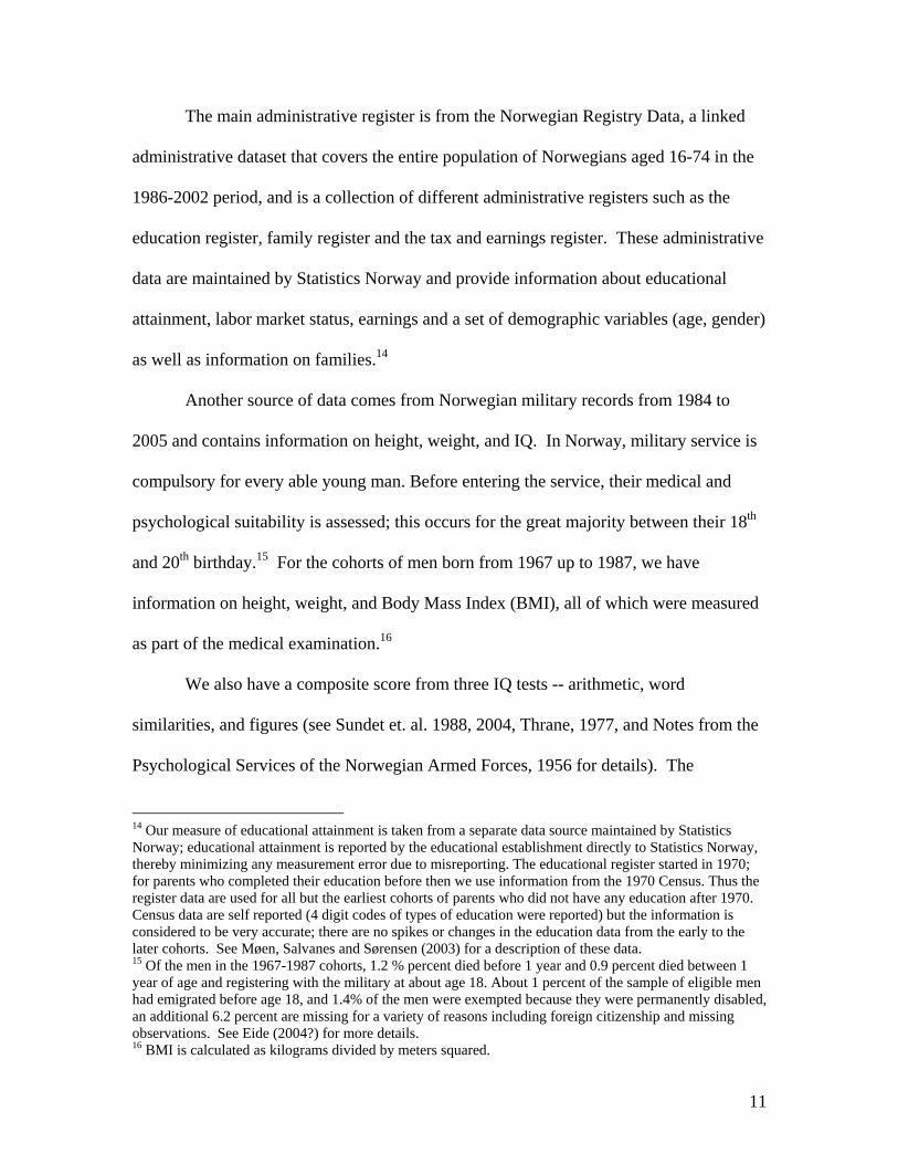
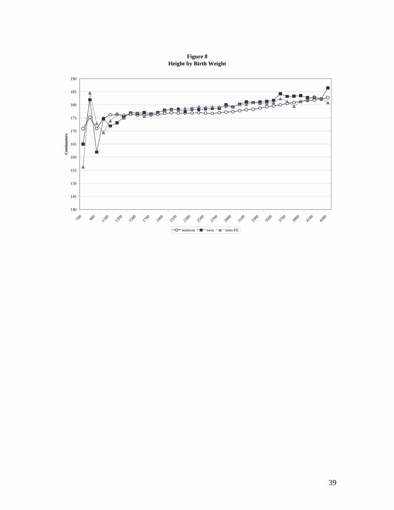
Table 4 shows the strong positive effects of birth weight on height, BMI, and
IQ.31 Height is measured in centimeters so the OLS estimate suggests that 1000 extra
grams at birth translates into about 2 extra centimeters of height at around age 18, and an
increase in BMI of around .4.32 Our IQ measure is on a scale from one to nine; the
estimated coefficient of 0.2 suggests that an increase in birth weight of 1000 grams will
increase the score by one- fifth of a stanine (or 1/10th of a standard deviation).
Given that BMI is an ambiguous health measure, as health may be adversely
affected if BMI is too high (so men are overweight) or BMI is too low (so men are
underweight), we have used the Center for Disease Control (CDC) cutoffs for overweight
(BMI greater than or equal to 25 – 11% of the twins sample) and underweight (BMI less
than 18.5 – 8% of the twins sample) to analyze the effect of birth weight on the
probability of being in either of these two groups (Results presented in Appendix Table
2). The fixed effects estimates show that increased birth weight increases the probability
of being overweight but decreases the probability of being underweight. Interestingly,
there is no significant effect on the probability of being in the recommended BMI
range.33
Heterogeneous Effects
32 There is an extensive literature suggesting that height is a useful indicator of health, both in developed as well as developing nations. See Strauss and Thomas (1998) for references. 33 Figures 8-10 show the OLS versus Fixed Effect averages for each of the military outcomes. Consistent with the other adult outcomes, the OLS and Fixed Effect estimates are quite similar. Also consistent is the absence of evidence of a non-linear relationship. This suggests that using cutoffs such as <1500 grams or <2500 grams as the variable of interest may not be appropriate for this type of analysis. 36 In the absence of control variables, this IV estimator is the well-known Wald estimator in which the effect of birth weight is calculated as the average difference in outcome between heavier and lighter twins divided by the average difference in birth weight between heavier and lighter. Unlike fixed effects, the Wald estimator is consistent as the number of twin pairs goes to infinity even in the presence of measurement error in birth weight.

21
While we included measures such as the natural log of birth weight in order to
allow for nonlinear effects, we also estimate the effect of birth weight for these outcomes
allowing for splines in birth weight with less than 1500, 1500-2500, and 2500 or more as
the cutoffs. These results are presented in the last rows of Tables 4 and 5. It is clear
there are substantial non-linearities in mortality, with a large marginal benefit for
additional grams among very low birth weight babies in terms of mortality. However, as
is further demonstrated in Figures 7-10, there is little evidence of significant linearities in
later outcomes.
Alternative Approach to Twin Fixed Effects
As an alternative approach to the twins fixed effect methodology that “differences
out” the twin-specific fixed effects, we could instead treat the “twin” effect as a random
variable that is part of the error term and correlated with birth weight; in this case, we
would need a credible instrument for consistent estimation of the effect of birth weight on
children’s outcomes. Any candidate instrument must differ in value within twin pairs, be
correlated with birthweight, and also be excludable. One candidate is an indicator
variable for whether the child is the heavier of the two twins, as this is correlated with
birth weight, differs between the two twins, and is, by construction, uncorrelated with the
twin random effect. The benefits of this approach are that it is much less parametric (as it
is essentially a difference in means or conditional means) and is much less susceptible to
measurement error.36 The cost is that it does not use all available information and, as a
result, is less efficient than fixed effects.

22
We implement this technique as a “robustness check” of our results. Table 6
presents the results when we regress the outcome on the birth weight in our sample of
same-sex twins (by sex) and instrument birth weight with an indicator for the heavier
twin (cases where both twins have the same weight are excluded). The regressions also
include the full set of control variable used in the pooled OLS regressions earlier. We
find reassuringly that the IV coefficient estimates are very close to the fixed effects
estimates in Tables 4 and 5 for both men and women. This suggests that our results are
robust to outliers and measurement error in the birth weight data. As expected, the
standard errors are higher than in the analogous fixed effects regressions.
Selection into the Sample
A final concern is that, when looking at the effect of birth weight on later
outcomes, we are inherently only including those individuals for whom we observe later
outcomes. In particular, individuals who did not live will not be included in our sample.
To the extent that birth weight may affect mortality, this may bias our results estimating
the effect of birth weight on later outcomes. Given that there is evidence that selection
into the sample may be changing over time (See Figures 3 and 4 for evidence of declining
mortality rates over time), it is important to understand how it may be affecting our
results.37
Though it is inherently impossible to know the effects of birth weight on the later
outcomes of the individuals we do not observe, we do think about this selection from
37 We have estimated the effect of birth weight on mortality separately for the sample used in our analysis of later outcomes. These results are presented in Appendix Table 3 and are similar to those from the full sample period.

23
three perspectives. First, from a theoretical perspective, if there are heterogeneous effects
of birth weight across twin pairs, and if there is a positive correlation between the effects
of birth weight on early and later outcomes, we would expect that twin pairs that
experience mortality are pairs for which birth weight would also be disproportionally
important for later outcomes. This reasoning suggests that early mortality will tend to
reduce the estimated effect of birth weight on later outcomes.
As another approach, we consider another intermediate outcome that is observed
for the entire sample and see if the effect of birth weight on the sample that die is
significantly different from the effect of birth weight on the sample that live. If the effect
of birth weight on this intermediate outcome is the same for the sample who lived and
those who did not, then one might believe that the effect of birth weight on the later
outcomes would also be the same. Beginning in 1977, we observe the apgar score for all
individuals. As a check, we estimate the relationship between birth weight and apgar for
twin pairs with and without mortality separately; when we do this using twin fixed
effects, we find that birth weight has a significantly larger positive effect on the apgar
score for twin pairs that subsequently experience mortality. If this relationship is also
true of other, later outcomes, then we may be underestimating the true effect of birth
weight on later outcomes.
Finally, a formal approach to the missing data problem is to model the probability
that a twin pair will experience mortality within the first year and hence attrit from the
later outcomes sample. We allow the probability of attrition to depend on the variables
that are always observed which we denote as xit (which includes all the usual control
variables plus the birth weight of each twin, and indicator variables for whether each twin

24
is LBW), but do not allow dependence on the variables that are missing for some units
(the later outcomes). The estimation of the model is carried out in two steps. In the first
stage, we estimate a probit model that conditions the probability of attrition on xit. The
predicted probabilities from the probit model are used to form weights and these weights
are used to weight the observations in the twin fixed effects estimation in the second step.
The weights are equal to the inverse of the probability of not attriting due to mortality in
the first year.38 When we do this reweighting, we again find that our estimates are likely
underestimating the true effect of birth weight on later outcomes.
6. Mitigating Effects
Given that there are clearly long-run effects of birth weight differences, the next
natural question is whether or not parents are able to offset these effects. Parents with
more resources may be better able to mitigate the negative effects of being born smaller.
Consistent with this idea, Currie and Gruber (1996) study the effects of Medicaid benefits
on prenatal care and conclude that targeted increased benefits had a much larger effect on
birth outcomes than broader expansions of eligibility to women with higher income
levels. This result indicates that parental income matters for birth outcomes. The
question we are asking is whether income also may offset the effect of low birth weight.
To examine this, we break our sample by mother’s education (less than high
school and high school or more) and examine the effects of birth weight separately by
38 This is referred to as Missing at Random (Little and Rubin, 1987). The argument is that there is nothing in the data that suggests that units that drop out are systematically different from units who do not drop out once we condition on all observed variables. This model has some intuitive appeal. Consider a unit that drops out in the first year with values of the observed variables equal to itit xX = . The Missing at Random assumption implies that for our best guess of the value of the missing later outcome variables, we should look at values of the later outcomes for units with the exact same values of xit.

25
group. These results are presented in Tables 7 and 8. From these tables, no clear pattern
emerges: there is little evidence that parental resources have a mitigating effect on child
outcomes. Indeed, one year mortality has a significant and somewhat larger effect for
children of higher-educated women (even after we have controlled for education and age
dummies). There are some indications for men that the longer run effects on high school
completion and earnings are observed primarily among the children of lower educated
mothers, but the opposite conclusion holds for height and BMI. There is little evidence of
any pattern for women.39
7. Generalizability
While using within twin variation allows us to credibly identify the causal effect
of birth weight on later outcomes, the question as to how generalizable these results are to
the general population of births remains.
From Table 1, we can see that there are substantial differences between twin and
singleton births. Not surprisingly, non-twins are on average heavier, with only 4 percent
classified as low birth weight (less than 2500 grams), while 39 percent of twins are low
birth weight. Gestation is also longer for singletons, with the average at 39.8 weeks
versus 36.9 for twins. Both one minute and five minute apgar scores are also higher,
there are a lower fraction with complications, and the one-year mortality rate is only 7.7
per 1000 births as opposed to 33 for twins. Parental education is the same but the
mothers of twins tend to be older.
39 We are, however, reluctant to draw too many inferences from these findings. Norway is a much more socialized country with much more income equality. It may be the case that, in Norway, society, and not parents, is the force that helps mitigate the negative effects of low birth weight.

26
One of the most notable differences is that twins come disproportionately from
the lower part of the birth weight distribution; this can be seen in Figure11, which shows
the distribution of birth weight for twins and non-twins. The question then becomes, are
twins and singletons similar controlling for birth weight? To examine this, we have
graphed the relationship between birth weight and mortality, education, height, BMI, and
IQ for the sample of twins and non-twins. (See Figures 6-10.) It is interesting to note
that the twins and non-twins actually have quite similar outcomes conditional on birth
weight, suggesting that our results may be generalizable to the rest of the population.
This is consistent with findings in the medical literature that suggest that the primary
cause of disparities in outcomes between twins and singletons is due to differences in size
at birth. Allen (1995) notes that, in a sample of pre-term births, no differences were
present between twins and singletons with respect to neurodevelopmental outcomes at 18
months from due date, after adjusting for confounding social, obstetric and neonatal
factors.40
8. Conclusions
Understanding the role of birth weight in child development and ultimate success,
very little is known about this relationship. In this paper, we have examined the effect of
birth weight on adult outcomes using within-twin variation in birth weight to control for
other often unobservable parental and environment factors. Even when comparing within
twin pairs, birth weight does seem to affect health and intelligence measures, with
significant positive effects. In addition, these health effects are translated into
40 Differences were only found when they examined pre-term infants with birth weights of <800 grams, suggesting greater vulnerability of twins born at the limit of viability. See Hoffman and Bennett (1990)

27
improvements in long run labor market outcomes such as education (particularly high
school completion) and earnings. In contrast with our short-run outcome, longer-run
outcomes do not appear to be smaller when a twins fixed effects methodology is used.
To get a perspective as to how large these coefficients are, we do a simple back-of-the-
envelope calculation using estimates from Currie and Moretti (2003). They find that one
year of extra maternal education reduces the probability of having a low birth weight
child by 1 percentage point from a baseline of about 5% of children being born LBW. If
we use this simple indicator and estimate the effect of being low birth weight on our
outcome measures, we can then calculate the effect of increasing mother’s education on
children’s outcomes through increasing birth weight. When we do this, we get that 1
year of maternal education increases male earnings by approximately .067% (FE) and
.178% (IV). In either case, the impact of one extra year of education is a fraction of a
percentage point in annual earnings and an even smaller effect on FT annual earnings.
Likewise, for men, FE implies one year of education increases height by .01 centimeters,
and IV suggests .03 centimeters. For women, one year of education increases the
probability of graduating high school by .0004 (FE) or .0014 (IV). Overall, these
numbers suggest that the impact of one extra year of maternal education coming through
birthweight on later outcomes is very small. However, magnitudes may be larger if we
were able to use a more continuous measure of birth weight, as our evidence suggests
there is little effect of the 2500 gram cutoff on longer run outcomes.
Our results suggest that birth weight does matter. Consistent with the recent
literature, we find little if any relationship between birth weight and mortality, and OLS
estimates greatly overestimate the true causal relationship. However, conclusions drawn

28
from these results can be misleading, for we find a significant impact of birth weight on
later outcomes of children, including height, BMI, and IQ, all at age 18, education, and
earnings. Additionally, we find that the relationship is remarkably linear, suggesting that
earlier work using indicators for low birth weight (<2500 grams) and very low birth
weight (<1500 grams) may be misspecified. Finally, we find little evidence that parents
are able to offset these negative effects of birth weight.

29
References
Allen, M.C. (1995), “Factors Affecting Developmental Outcome” in Multiple Pregnancy: Epidemiology, Gestation & Perinatal Outcome. Keith, Papiernik, Keith, and Luke, eds. Parthenon Publishing: New York.
Barker, D. J. (1995), “Fetal Origin of Coronary Hearth Disease, “ British Medical
Journal, Vol. 317, 171-174. Behrman Jere R., and Mark R. Rosenzweig (2004), “Returns to Birth weight”, Review of
Economics and Statistics, May, 86(2), 586-601. Black, Sandra E., Paul J. Devereux, and Kjell G. Salvanes (2005), “The More the
Merrier? The Effects of Family Size and Birth Order on Children’s Education”, Quarterly Journal of Economics, May.
Black, Sandra E., Paul J. Devereux, and Kjell G. Salvanes (2005), “Why the Apple
doesn’t Fall Far: Understanding Intergenerational Transmission of Education”, American Economic Review, March.
Bryan, Elizabeth (1992), Twins and Higher Order Births: A Guide to their Nature and
Nurture, London, UK: Edward Arnold, 1992). Case, Anne, Angela Fertig, and Christina Paxson, “The Lasting Impact of Childhood
Health and Circumstance.” Princeton Center for Health and Wellbeing Working Paper, April 2004.
Conley, Dalton, and Neil G. Bennett (2000), “Is Biology Destiny? Birth Weight and Life
Chances”, American Sociological Review, 65 (June), 458-467. Conley, Dalton, Kate Strully, and Neil G. Bennett (2005?), “A Pound of Flesh or Just
Proxy? Using Twin Differences to Estimate the Effect of Birth Weight on (Literal) Life Chances”, mimeo.
Currie, Janet and Jonathan Gruber (1996). “Saving Babies: The Efficacy and Cost of
Recent Changes in the Medicaid Eligibility of Pregnant Women.” Journal of Political Economy, Vol 104, No 6, pp. 1263-1296.
Currie, Janet, and Rosemary Hyson (1998), “Is the Impact of Health Shocks Cushioned
by Socio-Economic Status? The Case of Low Birth weight”, mimeo. Currie, Janet, and Enrico Moretti (2003), “Mother’s education and the Intergenerational
Transmission of Human Capital: Evidence from College Openings,” Quarterly Journal of Economics, CXVIII, 1495-1532.

30
Currie, Janet, and Enrico Moretti (2005), “Biology as Destiny? Short and Long-Run Determinants of Inter-Generational Correlations in Birth Weight”, mimeo.
Eide, Martha G., Nina Øyen, Rolv Skjærven, Stein Tore Nilsen, Tor Bjerkedal and
Grethe S. Tell (2005). ”Size at Birht and Gestational Age as Predictors of Adult Height and Weight, “ Epidemiology, Vol. 16 (2), 175-181.
Grjibovski, A. M., J. H. Harris and P. Magnus (2005). “Birthweight and adult health in a
population-based sample of Norwegian twins,” Twin Results and Human Genetics, Vol. 8(2), 148-155.
Hack, Maureen, Daniel J. Flannery, Mark Schluchter, Lydia Cartar, Elaine Borawski, and
Nancy Klein (2002). “Outcomes in Young Adulthood for Very-Low-Birth weight Infants.” New England Journal of Medicine, Volume 246, Number 3, January 17, 2002, 149-157.
Hack, Maureen, H. Gerry Taylor, Nancy Klein, Robert Eiben, Christopher
Schatschneider, and Nori Mercuri-Minich (1994) “School-Age Outcomes in Children with Birth Weights under 750 grams.” New England Journal of Medicine, Volume 331: 753-759. Number 12.
Hoffman, E.L. and F.C. Bennett (1990). “Birth Weight Less than 800 Grams: Changing
Outcomes and Influences of Gender and Gestation Number.” Pediatrics, 86, 27. Ijzerman, Richard G., Coen D.A. Stehouwer, and Dorret I. Boomsma (2000). “Evidence
for Genetic Factors Explaining the Birth Weight—Blood Pressure Relation: Analysis in Twins.” Hypertensions. Volume 36: 1008-1012.
Keith, Louis G., Emile Papiernik, Donald M. Keith, and Barbara Luke, editors. (1995)
Multiple Pregnancy: Epidemiology, Gestation, & Perinatal Outcome. Parthenon Publishing: New York.
Ment, Laura R., Betty Vohr, Walter Allan, Karol H. Katz, Karen C. Schneider, Michael
Westerveld, Charles C. Duncan, an drobert W. Makuch (2003). “Change in Cognitive Function Over Time in Very Low-Birth-Weight Infants.” Journal of the American Medical Association, Volume 289, Number 6, pp 705-711.
Sundet, Martin Jon, Dag G. Barlaug, and Tore M. Torjussen (2004), "The End of the
Flynn Effect? A Study of Secular Trends in Mean Intelligence Test Scores of Norwegian Conscripts During Half a Century", Intelligence, 32, 349-362.
Strauss, John and Duncan Thomas. (1998) “Health, Nutrition, and Economic
Development.” Journal of Economic Literature, Vol. 36, No. 2 (June) 766-817.

31
Christensen K, J.W. Vaupel, N. V. Holm, A.J. Yashin (1995). “Mortality Among Twins After Age 6: Fetal Origions Hypothesis Versus Twin Method.” British Medical Journal Vol. 319, 432-36.
Duffy, D.L. (1993). “Twin Studies in Medical Research.” Lancet Vol 341, 1418-19. Duffy, D. L. N. G. Martin, D. battisma, J. L. Hopper, J. D. Mathews (1990). “Genetics
and Astma and Hay Fever in Australian Twins.” American Review of Respiratory Disease, Vol 142, 1351-58.
Phillips, D.I.W. (1993). “Twin Studies in Medical Research : Can They Tell Us whether
Diseases are Genetically Determined? Lancet Vol. 334, 1008-9.

32
Figure 1Distribution of Differences in Birth Weight of Twins
23.92
18.78
15.02
12.25
8.79
7.12
4.423.39
1.93 1.6 1.06 0.6 0.37 0.25 0.16 0.14 0.07 0.05 0.02 0.050
5
10
15
20
25
30
100 200 300 400 500 600 700 800 900 1000 1100 1200 1300 1400 1500 1600 1700 1800 1900 2000

33
Figure 2Fraction of Twin Births Out of All Births
0
0.002
0.004
0.006
0.008
0.01
0.012
0.014
0.016
0.018
1967
1968
1969
1970
1971
1972
1973
1974
1975
1976
1977
1978
1979
1980
1981
1982
1983
1984
1985
1986
1987
1988
1989
1990
1991
1992
1993
1994
1995
1996
1997
1998

34
Figure 3Fraction of Twin Births That Are Same Sex Twins
0.56
0.58
0.6
0.62
0.64
0.66
0.68
0.7
0.72
0.74
0.76
19671968
19691970
19711972
19731974
19751976
19771978
19791980
19811982
19831984
19851986
19871988
19891990
19911992
19931994
19951996
19971998

35
Figure 4One-Year Mortality Rates
Per 1000 Births
0
2
4
6
8
10
12
14
16
1967
1968
1969
1970
1971
1972
1973
1974
1975
1976
1977
1978
1979
1980
1981
1982
1983
1984
1985
1986
1987
1988
1989
1990
1991
1992
1993
1994
1995
1996
1997

36
Figure 5Mortality Rates by Twin Status
per 1000 births
0
10
20
30
40
50
60
70
80
1967
1968
1969
1970
1971
1972
1973
1974
1975
1976
1977
1978
1979
1980
1981
1982
1983
1984
1985
1986
1987
1988
1989
1990
1991
1992
1993
1994
1995
1996
1997
twin mortality non-twin mortality

37
Figure 6Mortality Rate by Birth Weight
0
100
200
300
400
500
600
700
800
900
1000
500
700
900
1100
1300
1500
1700
1900
2100
2300
2500
2700
2900
3100
3300
3500
3700
3900
4100
4300
4500
4700
4900
5100
5300
5500
5700
5900
6100
6300
6600
Mor
talit
y (p
er 1
000
birt
hs)
non-twin twin twin FE

38
Figure 7High School Graduation by Birth Weight
0
0.1
0.2
0.3
0.4
0.5
0.6
0.7
0.8
0.9
1
700
900
1100
1300
1500
1700
1900
2100
2300
2500
2700
2900
3100
3300
3500
3700
3900
4100
4300
4500
non-twin twin twin-FE
39
Figure 8Height by Birth Weight
140
145
150
155
160
165
170
175
180
185
190
700
900
1100
1300
1500
1700
1900
2100
2300
2500
2700
2900
3100
3300
3500
3700
3900
4100
4300
Cen
timet
ers
nontwin twin twin-FE
40
Figure 9BMI by Birth Weight
0
5
10
15
20
25
30
700
9n
o
n
-
t
w
i
n
t w i nt w i n - F E


42
Figure 11Distribution of Birth Weight
0%
1%
2%
3%
4%
5%
6%
7%
8%
9%
0
200
400
600
800
1000
1200
1400
1600
1800
2000
2200
2400
2600
2800
3000
3200
3400
3600
3800
4000
4200
4400
4600
4800
5000
5200
5400
5600
5800
6000
6200
6400
Grams
nontwins twins

43
Table 1 Summary Statistics
Non-twins Sample
Twins Sample
Same Sex Twins Male
Same Sex Twins Female
Child’s Characteristics Infant Birth Weight Mean 3528
(558) 2598 (613)
2594 (639)
2540 (600)
Median 3540 2660 2660 2600 25th percentile 3210 2250 2240 2200 10th percentile 2880 1800 1750 1750 5th percentile 2640 1470 1380 1430 1st percentile 1860 820 760 800 Fraction low birth weight (<2500 Grams)
.03 (.17)
.33 (.47)
.33 (.47)
.36 (.48)
Gestation in weeks 39.83 (2.17)
36.90 (3.18)
36.62 (3.30)
37.02 (3.20)
Fetal Growth 88.46 (13.07)
69.83 (13.81)
70.14 (14.38)
68.05 (13.48)
1 minute APGAR score 8.68 (1.03)
8.21 (1.61)
8.14 (1.70)
8.22 (1.59)
5 minute APGAR score 9.29 (.75)
9.01 (1.10)
8.95 (1.19)
9.01 (1.10)
Fraction Female .49 (.50)
.50 (.50)
0 1
Fraction with Complications .31 (.46)
.49 (.50)
.49 (.50)
.49 (.50)
1 Year mortality rate (per 1000 births)
6.23 (78.69)
31.13 (173.67)
41.20 (198.75)
28.11 (165.30)
Mother’s Characteristics Education 11.43
(2.56) 11.53 (2.62)
11.55 (2.60)
11.53 (2.63)
Fraction <12 Years of Education .57 (.50)
.55 (.50)
.54 (.50)
.55 (.50)
Age 26.66 (5.23)
28.09 (5.11)
27.84 (5.11)
27.76 (5.18)
Fraction 30 or Older .28 (.45)
.38 (.49)
.36 (.48)
.36 (.48)
N 1,595,233 33,346 11,530 11,276 Apgar scores are only available after 1977; as a result, we have apgar scores for 959,518 nontwins, 21,708 twins, 7,540 for same sex male twins, and 7,243 for same sex female twins..

44
Table 2 Summary Statistics
Early Period (1968-1981) Non-twins
Sample Twins Sample
Same Sex Twins Male
Same Sex Twins Female
Child’s Characteristics Infant Birth Weight Mean 3511
(549) 2607 (616)
2650 (643)
2531 (602)
Median 3520 2660 2670 2590 25th percentile 3200 2250 2250 2180 10th percentile 2870 1810 1750 1740 5th percentile 2630 1480 1380 1440 1st percentile 1900 860 810 810 Fraction low birth weight (<2500 Grams)
.03 (.17)
.33 (.47)
.32 (.47)
.38 (.48)
Gestation in weeks 39.89 (2.16)
37.30 (3.28)
37.07 (3.38)
37.37 (3.32)
Fetal Growth 87.92 (12.85)
69.33 (13.78)
69.75 (14.35)
67.18 (13.38)
Fraction Female .49 (.50)
.50 (.50)
0 1
Fraction with Complications .24 (.43)
.44 (.50)
.44 (.50)
.43 (.50)
1 Year mortality rate (per 1000 births)
8.10 (89.63)
46.03 (209.55)
59.72 (236.98)
41.94 (200.47)
Percentage Completing High School
.73 (.45)
.73 (.43)
.73 (.44)
.75 (.44)
Earnings Data Earnings 260,132
(367,588) 257,092
(138,950) 300,639
(149,416) 210,709
(108,849) Earnings for Full Time Workers 311,616
(159,583) 307,463
(123,373) 337,016
(133,156) 262,239
(149,416) Military Data Height (Male Sample) 179.96
(6.51) - 179.33
(6.57) -
BMI (Male Sample) 22.50 (3.38)
- 21.84 (2.90)
-
IQ (Male Sample) 5.20 (1.79)
- 5.06 (1.82)
-
Mother’s Characteristics Education 10.76
(2.53) 10.69 (2.59)
10.77 (2.62)
10.69 (2.58)
Fraction <12 Years of Education .69 (.46)
.70 (.46)
.69 (.46)
.69 (.46)
Age 25.80 27.07 26.88 26.78

45
(5.27) (5.22) (5.23) (5.30) Fraction 30 or Older .22
(.42) .30
(.46) .29
(.45) .28
(.45) N 813,497 14,882 5,074 5,198

Table 3 Regression Results
Twins Sample
Mortality
High School Completion Ln(Earnings) Ln(Earnings) FT
OLS
FE OLS FE OLS FE OLS FE
Birth weight (1000s of grams)
-103.39** (3.92)
-9.67** (3.16)
.03** (.01)
.03** (.01)
.04** (.01)
.04* (.02)
.03** (.01)
.03** (.016)
Ln(Birth weight)
-279.16** (9.11)
-41.15** (7.64)
.08** (.02)
.09** (.04)
.10** (.03)
.09* (.05)
.07** (.02)
.10** (.04)
Fetal Growth -4.29** (.17)
-.41** (.12)
.002** (.0003)
.0012** (.0005)
.002** (.0004)
.0014* (.0008)
.001** (.0003)
.0012** (.0006)
N (clusters)
33,346 13,472 34,788 (5,858)
16,214 (3,893)

1
Table 4
Fixed Effects Regression Results Men-Same Sex Twins Sample
1-Year Mortality
High School Completion
Ln(Earn) Ln(Earn) FT Height BMI IQ
Birth weight (1000s of grams)
-8.02 (5.91)
.02 (.02)
.09** (.03)
.051** (.025)
2.18** (.22)
.39** (.12)
.21** (.07)
Ln(Birth weight)
-34.40** (14.08)
.06 (.06)
.24** (.08)
.15** (.07)
5.69** (.56)
1.12** (.30)
.62** (.18)
Fetal Growth
-.35 (.22)
.0007 (.001)
.003** (.001)
.002** (.001)
.08** (.01)
.015** (.004)
.008** (.003)
Splines:
BW<1500
-188.96** (39.90)
.47* (.27)
.17 (.24)
.21 (.23)
6.25** (2.39)
1.79 (1.28)
1.11 (.80)
1500<BW<2500
3.75 (12.91)
-.01 (.05)
.11* (.07)
.11* (.05)
2.67** (.50)
.69** (.27)
.47** (.16)
BW>2500
-3.34 (8.12)
.02 (.03)
.08* (.04)
.02 (.03)
1.86** (.29)
.22 (.16)
.07 (.09)
N (clusters)
11,530 4,486 12,057 (1990)
7,520 (1537)
5,388 5,378 4,926

2
Table 5
Fixed Effects Regression Results Female-Same Sex Twins Sample
1-Year Mortality High School Completion
Ln(Earn) Ln(Earn) FT
Birth weight (1000s of grams)
-10.93** (5.34)
.05** (.02)
-.02 (.04)
.02 (.02)
Ln(Birth weight)
-45.77** (12.59)
.13** (.05)
-.05 (.10)
.06 (.06)
Fetal Growth -.48** (.20)
.002** (.0008)
.-001 (.001)
.001 (.001)
Splines:
BW<1500 -341.87** (37.41)
.09 (.22)
-1.02 (.72)
1.57* (.68)
1500<BW<2500 17.01 (10.46)
.08* (.04)
.05 (.07)
-.01 (.04)
BW>2500 -9.81 (7.71)
.03 (.03)
-.04 (.05)
.01 (.04)
N (clusters)
11,276 4,762 12,031 (2070)
4192 (1193)

3
Table 6 IV Results
Same Sex Twins Sample 1-Year
Mortality High School Completion
Ln(Earn) Ln(Earn) FT Height BMI IQ
MEN Birth weight (1000s of grams)
5.31 (7.08)
.02 (.03)
.12** (.05)
.05 (.03)
2.13** (.29)
.40** (.15)
.19** (.09)
Ln(Birth weight)
13.15 (19.66)
.06 (.08)
.30** (.13)
.12 (.09)
5.57** (.77)
1.05** (.40)
.50** (.25)
Fetal Growth .20 (.29)
.001 (.001)
.004** (.002)
.0018 (.0013)
.08** (.01)
.015** (.006)
.007** (.0035)
WOMEN Birth weight (1000s of grams)
-17.45** (7.08)
.10** (.03)
-.06 (.06)
.02 (.04)
-- -- --
Ln(Birth weight)
-42.38** (17.19)
.26** (.07)
-.16 (.14)
.04 (.10)
-- -- --
Fetal Growth -.65** (.26)
.004** (.001)
-.002 (.002)
.001 (.001)
-- -- --

4
Table 7 Fixed Effects Regression Results Males- Same Sex Twins Sample
Low-Educated Mothers
1-Year Mortality
HS Completion
Ln(Earn) Ln(Earn) FT Height BMI IQ
Birth weight (1000s of grams)
-6.64 (8.46)
.04 (.03)
.11** (.03)
.07** (.03)
1.89** (.28)
.23 (.15)
.28** (.09)
Ln(Birth weight)
-42.28** (19.98)
.12 (.08)
.27** (.09)
.21** (.08)
5.13** (.71)
.74** (.37)
.73** (.23)
Fetal Growth -.32 (.31)
.0016 (.0011)
.004** (.001)
.003** (.001)
.07** (.01)
.01 (.006)
.01** (.003)
N (clusters)
6464 3096 9177 (1395)
5781 (1107)
3480 3490 3154
High Educated Mothers
1-Year Mortality
HS Completion
Ln(Earn) Ln(Earn) FT Height BMI IQ
Birth weight (1000s of grams)
-9.85 (8.05)
-.03 (.04)
.046 (.065)
-.002 (.050)
2.67** (.35)
.72** (.20)
.06 (.11)
Ln(Birth weight) -24.42 (19.42)
-.07 (.10)
.148 (.158)
-.001 (.116)
6.66** (.92)
1.92** (.52)
.40 (.30)
Fetal Growth -.41 (.30)
-.001 (.001)
.002 (.002)
-.0001 (.002)
.10** (.01)
.03** (.007)
.003 (.004)
N (clusters)
5066 1390 2539 (535)
1511 (379)
1908 1908 1772

5
Table 8 Regression Results
Females- Same Sex Twins Sample
Low-Educated Mothers 1-Year Mortality High School
Completion Ln(Earn) Ln(Earn) FT
Birth weight (1000s of grams)
-6.67 (7.71)
.05* (.027)
-.02 (.05)
.01 (.03)
Ln(Birth weight)
-32.03* (18.00)
.12* (.07)
-.02 (.12)
.04 (.07)
Fetal Growth -.31 (.29)
.002* (.001)
-.001 (.002)
.001 (.001)
N (clusters)
6344 3320 9006 (1449)
3012 (837)
High Educated Mothers
1-Year Mortality High School Completion
Ln(Earn) Ln(Earn) FT
Birth weight (1000s of grams)
-17.06** (7.03)
.05 (.03)
-.01 (.07)
.04 (.05)
Ln(Birth weight) -66.37** (16.81)
.16* (.08)
-.10 (.19)
.13 (.11)
Fetal Growth -.73** (.26)
.002* (.0013)
-.001 (.003)
.002 (.002)
N (clusters)
4932 1442 2583 (559)
1021 (316)

6
Appendix Table 1 Summary Statistics: Same Sex Twins
Same Sex Twins Heavier Lighter Infant Birth Weight Mean
2725 (615)
2414 (586)
Median 2800 2490 25th percentile 2400 2080 10th percentile 1940 1638 5th percentile 1570 1300 1st percentile 850
730
Fraction low birth weight (<2500 Grams) .26 (.44)
.43 (.50)
Fetal Growth
73.35 (13.39)
64.96 (13.23)
1 minute APGAR score
8.25 (1.59)
8.11 (1.69)
5 minute APGAR score
9.01 (1.11)
8.96 (1.16)
Fraction with Complications
.48 (.50)
.50 (.50)
1 Year mortality rate (per 1000 births) 32.65 (117.72)
34.97 (183.72)
N 11,180 Apgar scores are only available for 7,250 twins in our sample.

7
Appendix Table 2 Regression Results Male Twins Sample
Overweight Underweight Good Weight OLS FE OLS FE OLS FE Birth weight (1000s of grams)
.01 (.01)
.04** (.02)
-.03** (.01)
-.04** (.01)
.02* (.01)
-.001 (.02)
Ln(Birth weight)
.03 (.02)
.10** (.04
-.08** (.02)
-.11** (.04)
.05* (.03)
.01 (.05)
Fetal Growth .001* (.0004)
.0013* (.0006)
-.002** (.0004)
-.0013** (.0005)
.001* (.0005)
-.000 (.001)
N 5,378 5,378 5378

8
Appendix Table 2a Regression Results Male Twins Sample
Height BMI IQ OLS FE OLS FE OLS FE Birth weight (1000s of grams)
3.08** (.21)
2.18** (.22)
.23** (.09)
.39** (.12)
.18** (.06)
.21** (.07)
Ln(Birth weight)
7.51** (.55)
5.69** (.56)
.59** (.23)
1.12** (.30)
.49** (.14)
.62** (.18)
Fetal Growth .15** (.01)
.08** (.01)
.015** (.004)
.015** (.004)
.01** (.002)
.008** (.003)
N 5,388 5,378 4,926

Appendix Table 3 Regression Results: One Year Mortality
Twins Sample Early Period
(Mortality is measured as number of deaths per 1000 births) OLS FE Birth weight -146.45**
(6.35)
-1.99 (5.31)
Ln(Birth weight)
-390.13** (13.42)
-9.54 (12.98)
Fetal Growth -5.96** (.28)
-.06 (.20)
N 14,882