Embed Size (px)
Citation preview

Department of EconomicsWorking Paper 2016:14
The matching process: Search or mismatch?
Nils Gottfries and Karolina Stadin

Department of Economics Working paper 2016:14Uppsala University November 2016P.O. Box 513 ISSN 1653-6975 SE-751 20 UppsalaSwedenFax: +46 18 471 14 78
THE MATCHING PROCESS: SEARCH OR MISMATCH?
Nils Gottfries and Karolina Stadin
Papers in the Working Paper Series are published on internet in PDF formats. Download from http://www.nek.uu.se or from S-WoPEC http://swopec.hhs.se/uunewp/

1
THE MATCHING PROCESS:
SEARCH OR MISMATCH?*
Nils Gottfries# and Karolina Stadin##
24 November 2016
We examine the matching process using monthly panel data for local labour markets in Sweden. We find that an increase in the number of vacancies has a very weak effect on the number of unemployed workers being hired: unemployed workers appear to be unable to compete for many available jobs. Vacancies are filled quickly and there is no (or only weak) evidence that high unemployment makes it easier to fill vacancies; hiring appears to be determined by labour demand while frictions and labour supply play small roles. These results indicate persistent mismatch in the Swedish labour market.
Keywords: structural unemployment, frictional unemployment, matching function, labour demand, labour supply
JEL codes: J23, J62, J63, J64
*This paper builds on Chapter II in Stadin (2014). We are grateful for helpful comments on earlierversions from Timo Boppart, Mikael Carlsson, Per-Anders Edin, Anders Forslund, Håkan Gustavsson, John Hassler, Bertil Holmlund, Erik Mellander, Eran Yashiv, Johnny Zetterberg and seminar participants at Jönköping University, Nordic Summer Institute for Labor Economics, Ratio, the Riksbank (GSMG), and Uppsala University. We also want to thank employees at the Public Employment Service (Arbetsförmedlingen) for providing us with data and helpfully answering questions. Financial support from the Jan Wallander and Tom Hedelius Foundation and Marianne and Marcus Wallenberg Foundation is gratefully acknowledged.
# Department of Economics, Uppsala University, UCLS, CESifo and IZA, [email protected] ## Ratio and Uppsala Center for Labor Studies, [email protected]

2
1. Introduction
Vacancies and unemployment coexist in the labour market. In good times, there are many
vacancies and unemployment is low, while in bad times there are few vacancies and
unemployment is high. The standard explanation of these observations is that there are search
and matching frictions: it takes time for workers and firms to find each other. Normally,
search frictions are modelled with the help of a matching function, which is a reduced-form
relationship; the underlying microeconomic mechanisms are usually not spelled out.1
The word “search” suggests that frictions arise because of imperfect information. Workers are
imperfectly informed about jobs, and it takes time to contact firms and investigate job
opportunities. If vacancies and job seekers are trying to find each other within a finite space,
more vacancies should make it easier for unemployed workers to find jobs, and high
unemployment should make it easier to fill vacancies.
To this we can add heterogeneity and mismatch. Suppose that there are two types of jobs, A
and B, and two types of workers, A and B, and only A-workers can do A-jobs while only B-
workers can do B-jobs. Then, with a given probability of meeting, and equal numbers of each
type of worker and job, the flow of hiring will be half as large. If most workers are of type A
while most jobs are of type B, this will further reduce hiring for given stocks of
unemployment and vacancies. So, within this framework, changes in heterogeneity and
mismatch are expected to shift the matching function in a similar way as changes in search
intensity. In the standard search-matching literature, mismatch is typically thought of as one
factor that may cause a shift the matching function and the Beveridge curve; see, e.g., Daly,
Hobijn, Sahin and Valletta (2012) and Håkanson (2014).
1 For surveys of this literature, see Petrongolo and Pissarides (2001), Yashiv (2007) and Elsby, Michaels and Ratner (2015).

3
However, this way of thinking about heterogeneity and mismatch is still fundamentally based
on imperfect information. With perfect information, the A-workers will queue up for the A-
jobs, the B-workers will queue up for the B-jobs, and there will be excess supply, balance, or
excess demand in each submarket.
In this paper we investigate the matching process using a monthly panel from the Public
Employment Service (Arbetsförmedlingen) covering all 90 local labour markets in Sweden
1992:1-2011:12. Our focus is on how the hiring of unemployed workers and the filling of
vacancies are related to stocks of unemployment and vacancies at the beginning of the month
as well as to the inflows of vacancies and unemployed workers during the month.
As a background to our empirical study, we present two simple models of the labour market.
One is the standard matching function. The other is a model with perfect information where
unemployment is caused by persistent mismatch between supply and demand. In the latter
case, we assume that each local labour market consists of a mixture of submarkets, with
excess supply in some and full employment in other submarkets. Such a model is motivated
by the observation that in many markets – typically those for less skilled workers – there
appears to be constant excess supply while other markets have (close to) full employment –
typically those for highly qualified workers. We derive the implications of these two models
for the relations between the stocks and flows of vacancies and unemployment in a local
labour market. Compared to a standard matching function, a model with persistent mismatch
has very different implications for the relations between stocks and flows. First, if a large
fraction of the vacancies arise in markets with full employment, an increase in vacancies will
have a limited effect on the job prospects for unemployed workers. Second, and most
importantly, higher unemployment will not increase the rate at which vacancies are filled. The
reason is simple: in markets with unemployment, workers are queuing for the jobs and in
markets with full employment there is, by definition, no unemployment.

4
Our empirical findings point in the direction of persistent mismatch rather than information
problems as the main explanation of unemployment. More vacancies do lead to more
unemployed workers being hired, but the effect is surprisingly weak; it appears that only a
small fraction of vacancies are filled by unemployed workers. Higher unemployment does not
increase the rate at which vacancies are filled – or it has a weak effect in some specifications.
Our empirical results are in line with some recent empirical studies on macro and micro data.
Christiano et al. (2011) estimated a macro model where the recruitment cost per hired worker
could potentially depend on labour market tightness. However, they found no evidence that
recruitment costs depend on labour market tightness. Michaillat (2012) simulated a model
with wage rigidity and showed that, with reasonable parameter values, search frictions play a
small role in bad times but may be more important in a tight labour market. Michaillat and
Saez (2015) found that fluctuations in employment are mostly due to aggregate demand
shocks. Carlsson, Eriksson and Gottfries (2013) and Stadin (2015) used firm-level data and
found that higher unemployment does not make firms hire more workers.
Although many researchers have estimated matching functions, they have typically used more
limited data than we use and they have often imposed relatively tight specifications. Many
studies use aggregate data and assume the existence of a constant returns-matching function.
Thus, they relate the job finding rate to labour market tightness and since both variables are
pro-cyclical they find a positive regression coefficient. We do not impose CRS à priori;
instead we investigate the separate roles of vacancies and unemployment using panel data for
local labour markets. In our baseline estimation, we include fixed effects and time dummies to
reduce the risk of spurious correlations. Following the stock-flow matching literature, we
investigate the separate roles of inflows and initial stocks, and we estimate identical equations
with the filling of vacancies and the hiring of unemployed workers as dependent variables.

5
We find that the filling of vacancies and the hiring of unemployed workers are very different
variables; there is no such thing as a stable matching function that explains both of these
flows. Vacancies are filled quickly and, it appears, often by a worker who already had a job
(or was not in the labour force). Unemployed workers appear to be unable to compete for
many of the vacancies. We discuss previous empirical results in Section 6 and show that
qualitatively similar results have, in fact, been found in other studies when similar empirical
strategies were used.
Shimer (2007) brought renewed attention to heterogeneity and mismatch by explicitly
allowing for many separate submarkets and perfect competition within each submarket, so
that the number of matches is determined by the short side in each market.2 In Shimer’s
model, there is high mobility: jobs and workers move randomly between markets every time
they close/quit and because of this high random mobility, each worker has some chance of
matching with each vacancy. As a result, the two stocks are complements in the matching
process, and Shimer’s model produces a reduced-form relationship between stocks and flows,
that is similar to a Cobb-Douglas matching function (Shimer 2007, page 1093). We go to the
opposite extreme compared to Shimer (2007) and assume that workers cannot move between
markets and that there is constant excess supply in some markets and constant full
employment in other markets. Thus, our model highlights, starkly, the implications of a
persistent mismatch problem in terms of skills and experience. Our simple model yields a
different and testable prediction: vacancies will not be filled more quickly if there is high
unemployment, and this is also what we find in our empirical analysis. Obviously, a more
realistic model would allow for some mobility between markets and also for some markets to
switch from excess supply to balance or excess demand, but if heterogeneity is related to
skills and experience, this will be a slow process.
2 Shimer (2007) reviews some earlier work in this tradition. The model by Lagos (2000) is closely related.

6
So how can there be unemployment in some submarkets and full employment in other
submarkets? Clearly, there must be limited mobility among submarkets, and wage rigidity
may also play a role. In Shimer’s (2007) model, wages are flexible and adjust to clear each
submarket. If there are fewer jobs than workers in a particular submarket, wages fall to the
reservation wage and some workers are voluntarily unemployed. If there are more jobs than
workers, wages rise to equal productivity and all workers are employed. However, wages play
no role in the allocation of jobs and workers across submarkets; instead, the allocations of
jobs and workers are determined by exogenous random processes.3 Alternatively, we can
think of a model where wages affect the allocation but where they do not adjust enough to
clear each submarket. As in Lagos (2000), some markets are characterized by excess supply
(involuntary unemployment) while there is balance or a shortage of workers in other markets.
Figure 1 illustrates these two models of mismatch. In this paper, we do not take a stand on
what drives labour demand, how wages adjust, or whether unemployment is voluntary or
involuntary. The purpose of our simple model is to try to understand how labour market
stocks and flows are related when unemployment is caused by persistent mismatch rather than
imperfect information.
In Sections 2 and 3, we use a standard matching function and a simple model of mismatch
unemployment to derive equations for the hiring of unemployed workers and the filling of
vacancies. In Section 4, the data and the estimation method are presented, and we also
illustrate the relations between stocks and flows graphically. Section 5 contains the results of
the baseline econometric analysis, and in Section 6 we compare with previous studies. In
section 7 we consider alternative functional forms, and Section 8 concludes.
3 In an extension, Shimer (2007) allows for limited endogenous mobility, but this does not change the basic mechanism of the model.

7
Figure 1. Models of Mismatch
Shimer (2007)
Wage rigidity
L L
U
DA
DB WB
WA
L L
U
DA
DB
WA
WB

8
2. Frictional Unemployment
In this section, we specify a matching function that we estimate on monthly panel data from
the Public Employment Service. We take the effective number of job seekers to be
1in
t t tU u Eλ− + + where 1tU − is the number of unemployed workers who are registered at the
beginning of the month, intu is the inflow during the month and tE is the number of job
searchers who are not registered at the Public Employment Service. The parameter λ reflects
the importance of the inflow for the formation of matches. With random matching we would
expect λ to be smaller than unity because workers who enter during the period are available
for a shorter time than the workers who are looking for jobs already at the beginning of the
month. With stock-flow matching we may instead expect λ to be larger than unity so the
inflow matches at a higher rate than the initial stock. The stock-flow matching argument is
that the new inflow of workers can match with both the stock and the inflow of vacancies,
while the workers who were unemployed at the beginning of the month have already
exploited all matching possibilities with the vacancies that were available at the beginning of
the month.4 tE is unobserved and consists of two groups: job seekers without jobs who were
not registered as unemployed with the Public Employment Service and employed workers
searching on the job.5
Similarly, we take the effective stock of vacancies to be 1in
t t tV vθ− + +Ω where 1tV − is the stock
of vacancies that are registered at the beginning of the month, intv is the inflow of new
vacancies during the month and tΩ is the number of vacancies that are not registered at the
Public Employment Service. Using a similar argument as above, θ may be larger or smaller
4 Studies of stock-flow matching include Coles and Smith (1998), Gregg and Petrongolo (2005), Coles and Petrongolo (2008) and Ebrahimy and Shimer (2010). 5 Allowing the two types of job searchers to have different search intensities would not change the conclusions.

9
than unity depending on the matching technology. The matching function is specified as
follows:
( ) ( )1 1in in
t t t t t t t tM U u E V vα β
φ λ θ− −= + + + +Ω (1)
where tM is the total number of matches and we assume that and α β are smaller than
unity. We do not impose constant returns to scale because we see no compelling reason to do
so.6 The variable tφ represents variations in “matching efficiency,” which may be due to
changes in incentives, efficiency of the public employment service, and mismatch. With this
specification, the job-finding rate for someone who is unemployed at the beginning of the
period is ( )1/ int t t t tF M U u Eλ−= + + and hiring from registered unemployment is
( ) ( ) ( )1 1 1out in in int t t t t t t t tu F U u U u V v
α βλ λ θ ε− − −= + = + + (2)
where 1
1 1
1 1 .t tt t in in
t t t t
EU u V v
α β
ε φλ θ
−
− −
Ω= + + + +
The rate at which vacancies are filled is ( )1/ int t t t tQ M V vθ−= + +Ω so the number of registered
vacancies that are filled during the month is
( ) ( ) ( )1 1 1
1
1 1
where 1 1 .
out in in int t t t t t t t t
t tt t in in
t t t t
v Q V v U u V v
EU u V v
α β
α β
θ λ θ h
h φλ θ
− − −
−
− −
= + = + +
Ω= + + + +
(3)
6 If unemployed workers and firms search in a limited space we would expect increasing returns to scale in the meeting technology, but as pointed out by Petrongolo and Pissarides (2006) reservation wages may respond in such a way that an estimated matching function shows constant returns to scale.

10
The outflows of registered unemployed and vacancies are positively related to the registered
stocks, and the inflows and and t tε h are the unobserved parts. To test the predictions of the
model we estimate log-linearized versions of these equations:
11 1 12 13 1out
1t 4ln ln ln ln lnlnu in int t t t ta U a u a V a v ε− −= + + + + (4)
21 1 22 23 1out
2t 4ln ln ln ln lnlnv in int t t t ta U a u a V a v h− −= + + + + (5)
where 11 21 12 22 13 23 14 24, , and in in
in in in in
U u V va a a a a a a aU u U u V v V vα αλ β βθλ λ θ θ
= = = = = = = =+ + + +
.
Values without time indexes denote steady-state values. We chose to estimate a log-linear
specification as baseline because it is easy to understand and gives us a clear idea of how the
different variables are correlated.
Note that 11 12 21 22a a a a α+ = + = and 13 14 23 24a a a a β+ = + = so the deep parameters
and α β could potentially be inferred from the estimates.7 However, unregistered job
searchers and vacancies enter the error terms, and thus the estimated parameters may not
correspond to those of the underlying matching function. The bias depends on how the
unobserved variables co-vary with registered unemployment and vacancies. If on-the-job
search is either constant or pro-cyclical, ( )1/ int t tE U uλ− + will fall when unemployment
increases and since 1 0α − < this means that the estimated effect of unemployment on the
outflow from registered unemployment will be larger, i.e. the sum of the estimates 11 12a a+
will be larger than α . Furthermore, if tE increases when vacancies increase (pro-cyclical
7 Alternatively, we can think of these equations as log-linear approximations of the matching functions that arise in the stock-flow matching model – see equations 7-13 in Coles and Petrongolo (2008).

11
on-the job search), the net effect of vacancies on the outflow from registered unemployment
will be smaller; the sum of the estimates 13 14a a+ will be smaller than β .8
The effects of pro-cyclical on-the-job search on the coefficients in equation (5) go in the
opposite direction: the effect of registered unemployment on the vacancy outflow will be
smaller and the effect of vacancies increases. Thus, we see that pro-cyclical on-the-job search
changes the interpretation of the coefficients, but we would still expect all coefficient
estimates to be positive. For the effect of unemployment on the vacancy outflow to be zero,
an increase in unemployment would have to be fully countered by a decrease in on-the-job
search (see equation (1)), and this is unlikely.9 Simultaneity and measurement problems are
discussed in Section 4.
3. Mismatch Unemployment
In this section we present an alternative model with persistent mismatch of workers and jobs.
The basic idea is that each local labour market consists of many submarkets with specific job
characteristics and skill requirements. In some submarkets (type A), there are more workers
willing and able to work than there are jobs, and in other markets (type B) there is full
employment. We take demand for labour as given; what we attempt to understand is how
labour market stocks and flows are related when unemployment is caused by persistent
mismatch rather than search costs and information problems.
8 These biases are discussed in Petrongolo and Pissarides (2001). Whether search on the job is procyclical is not clear; Elsby, Michaels and Ratner (2015) construct a measure of on the job search and find it to be slightly countercyclical 9 If workers searching on the job face convex search costs and weigh the marginal benefits of search against the marginal costs, an increase in unemployment will make them search less, but not so much less that the effective number of job seekers decreases.

12
Demand, Supply, and Turnover
To match the empirical data, we let the period length be one month. There is a representative
firm and an exogenous labour force L in each market, and we let AtN and B
tN denote
employment at the end of the period in the two types of markets. In a market of type A, labour
demand is always smaller than L, firms can hire as many workers as they want and
unemployment is
A At tU L N= − . (6)
In the B-markets, all workers are employed, so BtN L= and 0B
tU = .
At the beginning of each period, some fractions and A Bt ts s of the employed workers quit their
jobs, or they are fired for exogenous reasons, and some fractions and zA Bt tz of the employed
workers decide to apply for other jobs and quit if they get new jobs. Then, firms in both
markets announce new vacancies and A Bt tv v resignations and hires occur, and workers
remain employed or unemployed until the end of the period. Vacancies remaining at the end
of a period are denoted AtV and B
tV .
Markets with Unemployment (type A)
We assume that a vacancy that exists at the beginning of the period generates Q hires during a
month and a vacancy that is announced during the month generates q hires during the month,
so hires in a market with unemployment are
1A A A
t t th QV qv−= + . (7)

13
We take the rates Q and q as exogenous, reflecting practical delays in collecting applications
and deciding whom to hire. It takes some time to hire a worker, but this time is independent of
the level of unemployment. We expect q to be smaller than Q because the new vacancies enter
during the period and thus have less time to be filled.
All workers who were unemployed at the beginning of the period and those who quit
exogenously search for jobs together with the workers who are trying to switch jobs. Firms
hire randomly among the job applicants, so the probability that a job searcher finds a job
during the month is
( )1 1 11
AA t
t A A A A A At t t t t t
hFU s N z s N− − −
=+ + −
. (8)
Markets with Full Employment (type B)
Even if there is full employment in markets of type B, it is normally possible to hire workers
because there are workers who are ready to switch jobs. Vacancies can be filled by those who
have already quit ( )Bts L and those who have not yet quit but are applying for other jobs
( )( )1 B Bt ts z L− . Assuming that
1Q qB Bt tV v− + workers are hired if there are applicants to all jobs,
hiring in the typical B-market is
( )( )( )1min Q q , 1B B B B B Bt t t t t th V v s s z L−= + + − . (9)
If there are enough applicants for all jobs, hiring will be equal to 1Q qB B
t tV v− + , but there could
also be congestion if there are not enough workers willing to switch jobs. This function is
kinked and concave. With some heterogeneity across markets, hires will be a smooth concave
function of the effective number of vacancies.

14
Outflow from Unemployment
The above equations describe a simple model of persistent mismatch. But we do not have data
for individual submarkets, so we need to understand the implications of the model for data on
a local labour market consisting of many submarkets. Thus, we assume that there is a
continuum of submarkets and that a fraction λ of the markets are markets with full
employment (type B). Then, aggregate unemployment at the end of the period is
( )1 At tU Uλ= − , (10)
the inflow into unemployment is
( ) 11in A At t tu s Nλ −= − (11)
and the outflow from unemployment is
( ) ( )1 11out A A A At t t t tu F U s Nλ − −= − + . (12)
Using (10), (11), (12), (8) and (7) we can write the outflow from unemployment as
( ) ( )( )( ) ( )
11
1
1
1 1 /
A At tout A in
t t t t A A int t t t
QV qvu F U u
z z L U u
λ
λ−
−−
− += + =
− + − +. (13)
The outflow from unemployment increases with the initial stock and with the inflow into
unemployment and the function is concave because unemployed workers compete with each
other for jobs.10 As in the frictional model, hiring from unemployment increases with
unemployment, but not because more unemployed workers can locate more jobs. Rather, the
reason is that the unemployed get some of the jobs that would otherwise have gone to the job
switchers.
10 As 1
int tU u− + approaches its maximum, ( )1 Lλ− , the outflow approaches ( )( )11 A A
t tQV qvλ −− + .

15
The outflow from unemployment increases with the number of vacancies – but only if the
vacancies appear in the markets where the unemployed workers are. Vacancies in markets
with full employment ( )1 and B Bt tV v− will not increase the job chances of unemployed workers.
Thus, the effect of an increase in total vacancies on the outflow from unemployment will
depend on where the vacancies appear.
Outflow of Vacancies
The outflow of vacancies is
( )( ) ( )( )( )1 11 min Q q , 1out A A B B B Bt t t t t t tv QV qv V v s s z Lλ λ− −= − + + + + − (14)
The outflow of vacancies will increase with the inflow and the initial stock of vacancies, and
this function may be linear or concave depending on whether there are enough workers
willing to switch jobs.
An important implication of this model is that variations in unemployment have no effect on
the rate at which vacancies are filled. Intuitively, this follows from two observations:
• in markets with unemployment, vacancies are filled at given rates;
• in markets with full employment, there is, by definition, no unemployment.
This prediction differs markedly from the implications of the matching function. If
unemployment is due to information frictions, the presence of more unemployed job seekers
should always increase the rate at which vacancies are filled.

16
4. Data and Estimation Method
We want to investigate how the hiring of unemployed workers and the filling of vacancies
during a month are related to the stocks of unemployment and vacancies at the beginning of
the month as well as the inflows of unemployed workers and vacancies during the month. We
begin by estimating equations (4) and (5), which are approximations of the matching function.
Alternative functional forms are considered in Section 7.
Data We use register data from the Public Employment Service (Arbetsförmedlingen) for the
period 1992:1-2011:12. Data from the Public Employment Service are available at the
municipality level at a monthly frequency. We aggregate the data to obtain a dataset with
variables for local labour markets, which consist of one or more municipalities and are
constructed by Statistics Sweden based on commuting patterns. Local labour markets are
constructed to be geographical areas that are as independent as possible from the rest of the
world with respect to labour demand and labour supply.11
The stock of unemployment, tU , is measured as the number of openly unemployed workers
that are registered at the Public Employment Service at the end of the month. There is a strong
incentive to register because doing so is required to qualify for unemployment benefits. In the
baseline estimation, workers in labour market program participants are not included because
earlier research indicates that they contribute to matching to a significantly smaller extent than
do openly unemployed workers; see Forslund and Johansson (2007). (We include program
participants in a robustness check.) The inflow into unemployment, intu , is measured as the
11 The 90 local labor markets are listed in the Appendix. Johansson and Persson (2000) reported that 80-90 percent of all hired workers came from the local labor market area where the firm was located. Survey data for vacancies and unemployment are not sufficiently large to allow panel estimation based on local labor markets.

17
number of workers who are newly registered as unemployed during the month and hires from
unemployment, outtu , are measured as the number of workers who left registered
unemployment, reporting to the employment service that they found jobs.
tV is the stock of vacancies registered at the Public Employment Service at the end of the
month, and intv is the inflow of new vacancies during the month. We measure the outflow of
vacancies as the inflow of new vacancies over the month minus the change in the stock:
( )outt t t-1V .Vin
tv v − −= (15)
A weakness of these data is that we do not know if all vacancies are filled. Firms may
abandon their recruitment efforts without actually hiring a worker and if the fraction of firms
that does this varies in a systematic way we may draw incorrect conclusions. 12
In our sample, unemployment was, on average, 7.2 percent of the labour force, the monthly
inflow into unemployment was 0.97 percent of the labour force and the outflow from
unemployment to jobs was 0.92 percent of the labour force; some of those who deregistered
did not report that they found a job. Vacancies were on average 0.53 percent of the labour
force, and the monthly inflows and outflows of vacancies were both 0.82 percent of the labour
force.13 Thus, the flows are similar but the stock of vacancies is more than ten times smaller
than the stock of unemployed workers.
Not all unemployed workers are registered at the Public Employment Service. According to
Aranki and Löf (2008), vacancies reported to the Public Employment Service corresponded to
30-45 percent of total hirings in the 1990s and 2000s. Thus, we should view our measures of
12 A recruitment survey, which is issued irregularly by the employer´s federation, shows that about 4/5 of all attempts to recruit result in hiring. 13 These are unweighted means across local labor markets. If we instead consider aggregate numbers, we find that unemployment was, on average, 6.2 percent and the monthly inflow into unemployment was 0.45 percent of the labor force, while vacancies were 0.54 percent and the monthly inflow of new vacancies was 0.42 percent of the labor force.

18
unemployment and vacancies as imperfect measures of the total stocks and flows of
unemployed workers and vacancies in the economy as a whole.
An important question, then, is how representative registered unemployed workers are of the
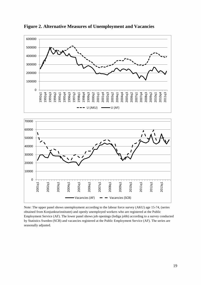
total population of unemployed workers. We have no direct evidence on this, but Figure 2
shows that, for Sweden as a whole, unemployment registered at the Public Employment
Service has fluctuated in a similar way as unemployment according to the labour force survey
conducted by Statistics Sweden (AKU). However, the number of unemployed workers that
are registered at the Public Employment Service has declined over time compared to the
survey measure.14 The lower panel in Figure 2 shows that aggregate vacancies registered at
the Public Employment Service (AF) are closely correlated with available jobs according to a
survey conducted by Statistics Sweden that began in the year 2001 (except for the first year of
the survey). The survey data are too limited to do analysis on the local labour market level.
Thus we see that, at the aggregate level, these measures vary similarly to the alternative
measures; they appear to be sufficiently broad and representative to make it worth studying
how stocks and flows are related. The long-term trend in the fraction of unemployed workers
that register at the employment service makes it important to account for underlying trends
and structural changes in the estimation.
14 Register data from the public employment service (AF) covers all persons registered at AF while the labour force survey (AKU) is a survey of about 30 000 persons. The difference between the different unemployment measures has been analysed by Statistics Sweden (Statistics Sweden 2016, Table 3). In 2015, 376 700 persons were unemployed according to AKU. Of these, SCB estimates that 133 600 were not registered at AF and 105 500 were participating in labour market programs with “activity support” so they were not openly unemployed according to AF. On the other hand, 34 700 persons who were registered as unemployed at AF would count as out of the labour force according to AKU, e.g. because they did not fulfil the job search requirement. There were also differences in the criteria used to count a person as employed, where AKU has stricter criteria, leading to a net difference of 18 700. In 2015, 191 100 persons were openly unemployed according to the public employment service: 376 700 133 600 105 500 34 700 18 700 191100.− − + + ≈
19
Figure 2. Alternative Measures of Unemployment and Vacancies
Note: The upper panel shows unemployment according to the labour force survey (AKU) age 15-74, (series obtained from Konjunkturinstitutet) and openly unemployed workers who are registered at the Public Employment Service (AF). The lower panel shows job openings (lediga jobb) according to a survey conducted by Statistics Sweden (SCB) and vacancies registered at the Public Employment Service (AF). The series are seasonally adjusted.
0
100000
200000
300000
400000
500000
60000019
92q1
1992
q419
93q3
1994
q219
95q1
1995
q419
96q3
1997
q219
98q1
1998
q419
99q3
2000
q220
01q1
2001
q420
02q3
2003
q220
04q1
2004
q420
05q3
2006
q220
07q1
2007
q420
08q3
2009
q220
10q1
2010
q420
11q3
U (AKU) U (AF)
0
10000
20000
30000
40000
50000
60000
70000
2001
q1
2002
q1
2003
q1
2004
q1
2005
q1
2006
q1
2007
q1
2008
q1
2009
q1
2010
q1
2011
q1
2012
q1
2013
q1
Vacancies (AF) Vacancies (SCB)

20
Estimation Method
To investigate how transition rates are related to stocks, we rely on differences in the variation
over time across local labour markets. Thus, we include time dummies and fixed effects for
local labour markets in our baseline specification. We include fixed effects because
geography, density, and industry structure affect the matching process in different labour
markets.
We include time dummies in the baseline specification for two reasons. First, cycles are
highly correlated across local labour markets, so although we have a panel with 90 local
labour markets, the results of a regression without time dummies will be driven mainly by the
aggregate business cycle. Then, there will be a risk that the results are affected by some
unobserved macroeconomic shocks that affected all local labour markets in the same way.
When we use differences in variation over time across labour markets, it is much less likely
that the results are affected by some specific unobserved shocks.
The second reason to include time dummies is that we have data for a long time period, and
there have clearly been structural changes in the labour market during this period. As
discussed above, there has been a decline in the fraction of unemployed workers that are
registered at the Public Employment Service. Additionally, formal rules and firms’ behaviour
– with respect to the posting of vacancies – may have changed. By including time dummies,
we can account for changes in rules and behaviour – provided that they had similar effects
across local labour markets.15
15 A number of structural changes have been noted in reports from the Public Employment Service: i) Until 2007, it was mandatory for all employers to announce their vacancies at the Public Employment Service, and this is still mandatory for the government. Although many vacancies went unreported before 2007, it is likely that this rule change affected firms’ behavior. ii) Around 2006-2007, there was an increased tendency for firms to post the same job several times, but from 2008 onward, such behavior was policed by the Public Employment Service. iii) In recent years, increased use of IT systems has led to a dramatic increase in automatic transfers of job postings to the PES register, and this appears to have increased the share of job postings that are registered with the PES. iv) Vacant summer jobs are posted earlier in the year in the latter part of the period.

21
We also include seasonal dummies interacted with dummies for the local labour markets. We
do this to account for differences in seasonal patterns depending on the importance of sectors
such as agriculture and tourism. Finally, we include local linear and quadratic time trends to
account for long-term structural changes in specific labour markets. Table 1 shows that there
is considerable variation remaining in the explanatory variables after removing fixed effects,
common time effects, and local seasons and trends.
Table 1. Standard Deviations of Explanatory Variables lnU lnV lnUin lnVin Variation removed: Fixed effects for llm, local seasons
0.403 0.706 0.308 0.505
Fixed effects for llm, local seasons, time dummies
0.160 0.563 0.206 0.453
Fixed effects for llm, local seasons, time dummies, linear and quadratic local time trends
0.114 0.539 0.181 0.414
Note: Stocks are measured on the last day of the previous month and in relation to the labour force. The inflows during the month are also measured in relation to the labour force in each local labour market. We estimate equations (4) and (5) by ordinary least squares (OLS) and instrument variable
estimation (IV). In the IV estimation, we use five lags of the inflows and the stocks from six
months ago as instruments. By instrumenting, we can alleviate two problems. First, there may
be purely random variation in the fractions of all unemployed workers and all vacancies that
register with the employment service. We can think of this as pure measurement errors that
will lead to biased estimates.16 Second, a simultaneity problem may arise because persistent
shocks to the matching function ( )tφ may be correlated with the variables included on the
right hand side. Suppose that there is a persistent increase in mismatch (e.g., because of a
16 The sign of this bias is unclear. If some additional vacancies are randomly registered and deregistered within the month, the inflow and outflow of vacancies will both increase. If some additional vacancies are randomly registered but not deregistered within the month, the inflow of vacancies will increase but not the outflow. If some vacancies are randomly deregistered, the outflow will increase but not the inflow.

22
large inflow of immigrants) so that the typical unemployed worker matches with fewer jobs.
This means that as tφ falls, the outflow from unemployment decreases and the stock of
unemployment increases over time. Persistent mismatch shocks of this type imply reverse
causation that will make the coefficient on the initial stock of unemployed smaller. To address
these problems, we use lagged stocks and inflows as instruments because they should be more
exogenous to the matching process in a given period than recent stocks and current inflows.17
A Look at the Data
Figure 3 shows vacancies, unemployment and the outflow from unemployment for the three
largest local labour markets: Stockholm, Göteborg and Malmö. The graphs for vacancies and
unemployment mirror each other and are fairly similar for the different local labour markets;
to a large extent, vacancies and unemployment reflect the general business cycle. The outflow
from unemployment is positively correlated with unemployment, but it is hard to see how it is
related to the number of vacancies.
Figure 4 shows the same data, aggregated to quarterly frequency, but here we have
unemployment on the horizontal axis and vacancies on the vertical axis, and the size of the
bubbles reflects the outflow from unemployment. By comparing the bubbles in the horizontal
direction, we can examine how the hiring of unemployed workers is related to the stock of
unemployed holding the stock of vacancies constant. We see clearly that the outflow from
unemployment is higher when unemployment is high. Comparing the sizes of the bubbles in
the vertical direction, holding unemployment constant, we see only a weak positive relation
between the number of vacancies and the outflow from unemployment.
17 Unfortunately, we have been unable to find more exogenous instruments. We tried to exploit the industry structure of different local labor markets, using input-output tables to construct exogenous shocks. Such an approach was used successfully by Carlsson, Eriksson and Gottfries (2013) for firm-level data. This approach was unsuccessful, however. Because of strong input-output linkages between different sectors, there turned out to be very little difference between the exogenous shocks calculated for different local labor markets.

23
Figure 3. Outflow from Unemployment
Note: Monthly register data from the Public Employment Service, seasonally adjusted.
-5.8
-5.6
-5.4
-5.2
-5-4
.8lnU
out
-7-6
-5-4
-3-2
lnU&l
nV
1990m1 1995m1 2000m1 2005m1 2010m1
lnU lnV lnUout
Stockholm
-6-5
.5-5
-4.5
lnUou
t
-7-6
-5-4
-3-2
lnU&l
nV
1990m1 1995m1 2000m1 2005m1 2010m1
lnU lnV lnUout
Göteborg
-5.6
-5.4
-5.2
-5-4
.8-4
.6ln
Uout
-7-6
-5-4
-3-2
lnU&
lnV
1990m1 1995m1 2000m1 2005m1 2010m1
lnU lnV lnUout
Malmö

24
Figure 4. Bubble Scatter Plots for Hiring from Unemployment 1992-2011 Larger bubble = larger outflow from unemployment
Note: Quarterly averages of monthly register data from the Public Employment Service, seasonally adjusted.
-6.5
-6-5
.5-5
-4.5
lnV
-4 -3.5 -3 -2.5lnU
Uout-bubbles Stockholm
-7-6
.5-6
-5.5
-5-4
.5ln
V
-4 -3.5 -3 -2.5 -2lnU
Uout-bubbles Göteborg
-6.5
-6-5
.5-5
-4.5
lnV
-3.5 -3 -2.5 -2lnU
Uout-bubbles Malmö

25
Figure 5 shows vacancies and unemployment for the three largest labour markets together
with the outflow of vacancies. The outflow of vacancies is very closely correlated with the
number of vacancies, but it is difficult to see whether the outflow of vacancies is related to
unemployment.
In Figure 6 we again have unemployment on the horizontal axis and vacancies on the vertical
axis, but now the size of the bubbles reflects the outflow of vacancies. By comparing the sizes
of the bubbles in the vertical direction, holding unemployment constant, we see that more
vacancies are associated with a bigger outflow of vacancies. Comparing the sizes of the
bubbles in the horizontal direction, holding vacancies constant, we see no obvious relation
between unemployment and the outflow of vacancies.
Our graphical examination indicates strong “own effects” in the sense that high
unemployment leads to a high outflow from unemployment and more vacancies lead to more
vacancies being filled. The “cross effects” appear weak, however. Hiring from unemployment
is only weakly related to the number of vacancies, and we see no clear relation between
unemployment and the rate at which vacancies are filled.
Note, however, that this graphical examination exploited the time series variation in
individual labour markets, so the results may be driven by common unobserved shocks and
structural changes. By including time dummies in our panel estimation we can eliminate the
effects of common shocks, and this should make the results more reliable. By IV estimation
we can reduce the effects of measurement errors and simultaneity.

26
Figure 5. Outflow of Vacancies
Note: Monthly register data from the Public Employment Service, seasonally adjusted.
-5.5
-5-4
.5-4
-3.5
lnVou
t
-7-6
-5-4
-3-2
lnU&l
nV
1990m1 1995m1 2000m1 2005m1 2010m1
lnU lnV lnVout
Stockholm
-6-5
.5-5
-4.5
-4lnV
out
-7-6
-5-4
-3-2
lnU&l
nV
1990m1 1995m1 2000m1 2005m1 2010m1
lnU lnV lnVout
Göteborg
-6-5.
5-5
-4.5
-4lnV
out
-7-6
-5-4
-3-2
lnU&ln
V
1990m1 1995m1 2000m1 2005m1 2010m1
lnU lnV lnVout
Malmö

27
Figure 6. Bubble Scatter Plots for the Outflow of Vacancies 1992-2011 Larger bubble = larger outflow of vacancies
Note: Quarterly averages of monthly register data from the Public Employment Service, seasonally adjusted.
-6.5
-6-5
.5-5
-4.5
lnV
-4 -3.5 -3 -2.5lnU
Vout-bubbles Stockholm
-7-6.
5-6
-5.5
-5-4.
5lnV
-4 -3.5 -3 -2.5 -2lnU
Vout-bubbles Göteborg
-6.5
-6-5.
5-5
-4.5
lnV
-3.5 -3 -2.5 -2lnU
Vout-bubbles Malmö

28
5. Results
Table 2 shows OLS and IV estimates of equations (4) and (5) with the outflow from
unemployment and the outflow of vacancies as dependent variables.
Table 2. Determinants of Outflows of Unemployed Workers and Vacancies
(1) (2) (3) (4) lnUout OLS lnUout IV lnVout OLS lnVout IV
lnU 0.576*** 0.585*** -0.012 0.103 (0.023) (0.053) (0.022) (0.071) lnUin 0.000 0.207*** -0.016 -0.065 (0.013) (0.060) (0.019) (0.083) lnV 0.009*** 0.013* 0.415*** 0.487*** (0.003) (0.007) (0.009) (0.018) lnVin 0.038*** 0.111** 0.462*** 0.821*** (0.005) (0.043) (0.013) (0.065) Observations 20,394 19,725 20,391 19,722 R-squared 0.853 0.845 0.799 0.731 Number of llm 90 90 90 90 Hansen (p-value) 0.220 0.973 Kleibergen-Paap (p-value) 0.000 0.000
Note: Robust standard errors (clustered on local labour market) in parentheses; *** p<0.01, ** p<0.05, * p<0.1. Fixed effects for local labour markets, time dummies, local seasons and linear and quadratic local time trends are included in all specifications. Instruments for IV are five lags of inflows plus the stocks in t-6.
Unemployment Outflow Equation According to the OLS estimates in column 1 of Table 2, unemployment and vacancies both
have statistically significant effects on the outflow from unemployment, but the stock of
unemployed workers has a quantitatively much larger effect than the effect of vacancies.
There is no effect of the inflow of newly unemployed workers. In column 2 we account for
measurement errors and simultaneity by instrumenting all the variables on the right hand side
with five lags of the inflows and the stocks lagged six months. The test statistics show that
this instrument set is both valid and relevant. One concern, which was raised above, is that

29
mismatch shocks may create a simultaneity problem that affects the coefficients for the
stocks, but this does not appear to be an important problem; the coefficients for the stocks are
roughly similar as we go from OLS to IV. The coefficients for the inflows increase, however,
and become quantitatively important when we estimate by IV. One possible interpretation is
that estimation by IV reduces the effects of measurement errors with respect to the inflows.
As discussed above, estimation by IV should be a good way to address measurement errors.
In the IV estimation, the sum of the coefficients for the stock and inflow of unemployment is
about 0.8, so a 10 percent increase in the stock and the inflow into unemployment will raise
the outflow by approximately 8 percent. A ten percent increase in (new and old) vacancies
increases hiring from unemployment by only 1.2 percent. The sum of the four coefficients in
column 2 is 0.916 and we cannot reject constant returns to scale at conventional levels of
significance. The signs of the effects are qualitatively in line with the implications of the
matching function, but the effect of vacancies on the hiring of unemployed workers is
surprisingly weak.
Vacancy Outflow Equation Column 3 in Table 2 shows the OLS estimate of equation (5) with the outflow of vacancies as
the dependent variable. We see that the initial stock and the inflow of new vacancies both
contribute to the outflow of vacancies, but neither the initial stock of unemployment nor the
unemployment inflow have significant effects on the rate at which vacancies are filled.
The IV estimates are shown in Column 4, and again the test statistics show that the
instruments are both valid and relevant. Compared to OLS, we find a much bigger effect of
the vacancy inflow, while the effect of the vacancy stock is somewhat larger. As discussed
above, this difference between OLS and IV could be due to measurement errors. Again, we
see no effect of unemployment on the vacancy outflow.

30
The sum of the coefficients in column 4 is 1.308 and we can reject constant returns to scale
statistically, so instead of congestion we find increasing returns to scale. One possible
interpretation is that this reflects heterogeneity among vacancies. There may be some fairly
constant sets of vacancies that are difficult to fill, while the vacancies that do fluctuate are
filled at a faster rate.18
Robustness across Time and Space In Table 3 we investigate the robustness of the results for the unemployment outflow across
time and space; all estimations are performed by IV, including local labour market fixed
effects, time dummies, local seasons and local trends. Column 1 repeats our baseline estimate
for the whole time period and all labour markets. In columns 2 and 3 we estimate the equation
for two periods, 1992-1999 and 2000-2011. The coefficient estimates are similar to what we
find for the whole period, but some coefficients are more uncertain and not statistically
significantly different from zero. In columns 4-6 we divide the sample into small, medium
and large labour markets, with one third of the labour markets placed in each category. The
results are qualitatively roughly similar those for the whole sample, but some estimates are
more uncertain.
In Table 4 we investigate the robustness of the results for the vacancy outflow across time and
space. The results are robust across time and space. In no case do we find any statistically
significant effect of unemployment, but the coefficients for the stock and inflow of vacancies
are stable showing significant, positive effects on the outflow of vacancies.
18 There are a large number of job openings in tele-marketing where payment is often based on commission and firms may simply want to hire as many as possible.

31
Table 3. The Outflow from Unemployment: Robustness across Time and Space Dep. variable: lnUout (1) (2) (3) (4) (5) (6)
Period 1992-2011 1992-1999 2000-2011 1992-2011 1992-2011 1992-2011 Labour markets All All All Small Medium Large
lnU 0.585*** 0.844*** 0.668*** 0.718*** 0.568*** 0.483*** (0.053) (0.193) (0.059) (0.095) (0.043) (0.084) lnUin 0.207*** 0.242 0.123 0.061 0.205** 0.278*** (0.060) (0.243) (0.084) (0.104) (0.100) (0.097) lnV 0.013* 0.022* 0.012** 0.009 0.022*** -0.003 (0.007) (0.011) (0.005) (0.012) (0.008) (0.013) lnVin 0.111** 0.144 0.098 0.079 0.104 0.218*** (0.043) (0.090) (0.066) (0.056) (0.069) (0.063) Observations 19,725 7,317 11,870 6,405 6,660 6,660 R-squared 0.845 0.859 0.826 0.801 0.870 0.921 Number of llm 90 90 90 30 30 30 Note: Robust standard errors in parentheses; *** p<0.01, ** p<0.05, * p<0.1. IV-regressions. Instruments: five lags of inflows plus the stocks in t-6. Regressions include fixed effects for local labour markets, time dummies, local seasons and local trends.

32
Table 4. The Outflow of Vacancies: Robustness across Time and Space
Dep. variable: lnVout (1) (2) (3) (4) (5) (6) Period 1992-2011 1992-1999 2000-2011 1992-2011 1992-2011 1992-2011
Labour markets All All All Small Medium Large lnU 0.103 -0.238 -0.024 0.168 -0.022 0.150 (0.071) (0.216) (0.075) (0.143) (0.098) (0.122) lnUin -0.065 0.464 0.013 -0.078 0.016 -0.105 (0.083) (0.344) (0.122) (0.174) (0.108) (0.135) lnV 0.487*** 0.428*** 0.536*** 0.498*** 0.479*** 0.446*** (0.018) (0.030) (0.018) (0.026) (0.026) (0.045) lnVin 0.821*** 0.884*** 0.578*** 0.886*** 0.610*** 0.796*** (0.065) (0.119) (0.115) (0.075) (0.123) (0.142) Observations 19,722 7,317 11,867 6,403 6,659 6,660 R-squared 0.731 0.779 0.791 0.665 0.791 0.854 Number of llm 90 90 90 30 30 30 Note: Robust standard errors in parentheses; *** p<0.01, ** p<0.05, * p<0.1. IV-regressions. Instruments: five lags of inflows plus the stocks in t-6. Regressions include fixed effects for local labour markets, time dummies, local seasons and local trends.

33
These robustness checks show that our main results are not due to some specific shocks that
happened in particular time periods or in specific labour markets. If we think of these
regressions as estimates of “the matching function,” two results are surprising. The first is that
the number of vacancies has such a weak effect on the hiring of unemployed workers. The
second is that unemployment has no effect on the outflow of vacancies. Both results are
consistent with a model of persistent mismatch in the labour market but inconsistent with a
standard matching function.
Our estimates tell us something important about vacancy data. There are many vacancies in a
boom, but this is not because their durations increase; instead, it is because there is a large
inflow of vacancies in boom periods.
One may argue that the latter result arises mechanically because firms routinely post
vacancies for a fixed time and then collect applications and hire the best applicant. However,
this is exactly how we would expect firms to behave if they expect to quickly attract a
sufficient number of qualified applicants for most jobs that they announce.
Alternative Trends, Aggregate Data and Labour market Programs Table 5 shows regressions where we leave out either the local trends or the time dummies.
The “cross effects” become positive in some cases and negative in other cases, but they are
generally weak. Without time dummies or without local trends, higher unemployment appears
to have a positive effect on the outflow of vacancies. However, the effect is quite small and of
limited economic significance. A one-standard-deviation change in both and inV v has an
effect on outv that is almost 10 times larger than the effect of one standard deviation changes in
both and u inU .19
19 Using the standard errors in the first row of Table 1 and the coefficients in the sixth column of Table 5, we get 0.133 0.403 0.088 0.308 0.081⋅ + ⋅ = for unemployment and 0.453 0.706 0.720 0.505 0.683⋅ + ⋅ = for vacancies.

34
Table 5. Leaving out Local Trends or Time Dummies
(1) (2) (3) (4) (5) (6) Baseline No trend No TD Baseline No trend No TD lnUout IV lnUout IV lnUout IV lnVout IV lnVout IV lnVout IV
lnU 0.585*** 0.416*** 0.811*** 0.103 0.152*** 0.133*** (0.053) (0.041) (0.038) (0.071) (0.037) (0.029) lnUin 0.207*** 0.328*** 0.083** -0.065 -0.100* 0.088*** (0.060) (0.057) (0.038) (0.083) (0.059) (0.031) lnV 0.013* 0.020*** -0.027** 0.487*** 0.488*** 0.453*** (0.007) (0.007) (0.013) (0.018) (0.017) (0.019) lnVin 0.111** -0.012 0.462*** 0.821*** 0.727*** 0.720*** (0.043) (0.025) (0.048) (0.065) (0.034) (0.041) Time dummies YES YES NO YES YES NO Local trends YES NO YES YES NO YES Observations 19,725 19,725 19,725 19,722 19,722 19,722 R-squared 0.845 0.820 0.645 0.731 0.749 0.741 Number of llm 90 90 90 90 90 90 Note: Robust standard errors in parentheses; *** p<0.01, ** p<0.05, * p<0.1. IV-regressions. Instruments: five lags of inflows plus the stocks in t-6. In baseline time dummies, local seasonal dummies, linear and quadratic local trends, and fixed effects for the local labour market are included.
35
Table 6. Estimation on Aggregate Data
(1) (2) (3) (4) lnUout OLS lnUout IV lnVout OLS lnVout IV lnU 0.627*** 0.748*** -0.055*** -0.070* (0.030) (0.047) (0.021) (0.039) lnUin 0.144*** 0.198** -0.111*** 0.035 (0.049) (0.100) (0.037) (0.067) lnV -0.160*** -0.284*** 0.137*** 0.103*** (0.026) (0.041) (0.020) (0.027) lnVin 0.485*** 0.715*** 0.761*** 0.889*** (0.035) (0.067) (0.027) (0.040) Observations 228 222 228 222 R-squared 0.964 0.956 0.985 0.981 Note: Robust standard errors in parentheses; *** p<0.01, ** p<0.05, * p<0.1. Seasonal dummies, linear and quadratic trends included. There is clear evidence of changes in the seasonal pattern and the public employment service has noted that summer jobs are announced earlier towards the end of the sample period. To account for this we include interaction terms between trends and season. (In the baseline panel estimation, common changes in seasonality are handled by the time dummies.)
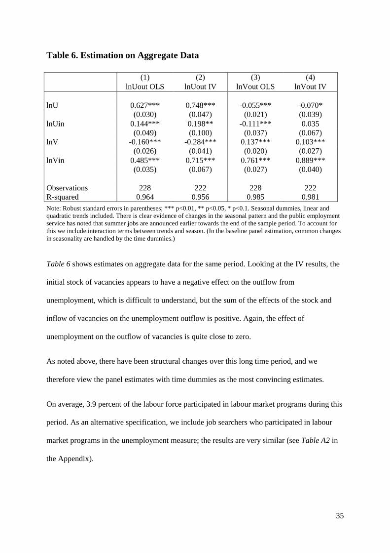
Table 6 shows estimates on aggregate data for the same period. Looking at the IV results, the
initial stock of vacancies appears to have a negative effect on the outflow from
unemployment, which is difficult to understand, but the sum of the effects of the stock and
inflow of vacancies on the unemployment outflow is positive. Again, the effect of
unemployment on the outflow of vacancies is quite close to zero.
As noted above, there have been structural changes over this long time period, and we
therefore view the panel estimates with time dummies as the most convincing estimates.
On average, 3.9 percent of the labour force participated in labour market programs during this
period. As an alternative specification, we include job searchers who participated in labour
market programs in the unemployment measure; the results are very similar (see Table A2 in
the Appendix).

36
6. Comparison with Previous Empirical Results
No/Weak Effect of Unemployment on the Outflow of Vacancies Our most striking result is that unemployment does not affect the rate at which vacancies are
filled – or it has a weak effect. Comparing to previous empirical results, we find it most
interesting to compare with studies which use similar methodology, i.e. panel studies where
the dependent variable is the filling of vacancies, constant returns to scale are not imposed
and the regressions include time dummies and fixed effects for the local or regional labour
market.20 Taking a close look at the literature, we find that some results that are similar to
ours have, in fact, been reported before.
Anderson and Burgess (2000) use a quarterly panel of four US states, and the dependent
variable is new hires according to register data. In most of their estimates, they do not include
seasonal dummies. When they include time effects (which pick up seasonality) the coefficient
for the log of unemployment is 0.19, but it is far from statistically significant. Furthermore,
they find a zero effect of unemployment on hires from non-employment (Table 2, columns 4
and 5 in their paper).
Kangasharju, Pehkonen and Pekkala (2005) use a panel very similar to ours, with monthly
data for Finland and filled vacancies as the dependent variable. Similar to our study, they
include both initial stocks and inflows as explanatory variables, and they include year
dummies, seasonal dummies and fixed effects. In fact, they find very similar results to ours,
reporting that “…matches are mainly driven by the demand side of the labour market … the
elasticity with respect to the stock of old vacancies is 0.3 and with respect to new vacancies
0.6. The corresponding effect from the supply side (job seekers) is only around 0.1.” With a
20 As discussed above, studies on aggregate data can easily generate spurious results, and pure cross section estimates such as Coles and Smith (1996) answer very different questions about how the size and density of the labor market affects the matching process.

37
translog specification they find a somewhat bigger role for the supply side, but it is still the
demand side that dominates.21
Borowczyk-Martins, Jolivet and Postel-Vinay (2013) estimate matching functions on JOLTS
data using all additions to the payroll as the dependent variable. In their baseline estimate,
they impose CRS so that the explanatory variable is tightness. When they relax CRS, their
OLS estimate gives a negative effect of unemployment on the number of matches (-0.280).
They also perform GMM estimation, finding an effect of unemployment that is positive but
far from statistically significant.
For Sweden, Edin and Holmlund (1991) estimated aggregate matching functions with the
outflow of vacancies as the dependent variable and initial stocks and a trend as explanatory
variables, finding coefficients of 0.23 for unemployment and 0.56 for vacancies. One reason
for the difference may be that they have data for the period 1970-1988, when unemployment
was much lower, while our sample begins with the crisis in the 1990s and there is slackness in
the labour market for large parts of the sample period. Finding workers should be more of a
problem when unemployment is low (Michaillat 2012). Running the same regression (with
only initial stocks) on aggregate data for the period 1992-2011, we obtain coefficients of -0.05
for the initial stock of unemployment (not significant) and 0.64 for the initial stock of
vacancies.
Small Effect of Vacancies on Hiring from Unemployment With hiring from unemployment as the dependent variable, we found positive coefficients for
unemployment and vacancies but the latter effect was surprisingly weak. It is interesting to
relate our results to the recent studies of stock-flow matching by Gregg and Petrongolo (2005) 21 There are typos in their Table 2. Hynninen (2005) estimates matching functions on monthly panel data for local labor markets in Finland using the outflow of vacancies as the dependent variable. A key difference is that she does not include the inflows on the right hand side and, for this reason, the estimates are not directly comparable. As seen from our estimates, the inflows help very much to explain the outflows, especially for vacancies.

38
and Coles and Petrongolo (2008). A key point they make is that the vacancies and job seekers
“at risk” are weighted sums of the initial stocks and the inflows and they also note that,
because of the high turnover of vacancies, the initial stock of vacancies is a poor proxy for the
vacancies “at risk”. In fact, they find that the inflow of vacancies is a more important
determinant of hiring from unemployment than the vacancy stock. This is also what we find
when we estimate by IV. According to our IV estimate in Table 2, column 2, a one-standard-
deviation increase in the vacancy inflow leads to a 5.6 percent increase in hiring from
unemployment ( )0.111 0.505 0.056⋅ = while a one standard deviation increase in the initial
vacancy stock leads to a 0.9 percent increase in hiring from unemployment
( )0.013 0.706 0.009⋅ = .22
In a study of aggregate data for Sweden, Forslund and Johansson (2007) used the hiring of
registered job seekers as the dependent variable. Measuring vacancies as the initial stock plus
half the inflow, they found a coefficient of approximately 0.2 for vacancies, which is a bit
higher than what we find. When estimating a stock-flow matching model they find, like Coles
and Petrongolo (2008) and the present study, and that the inflow of new vacancies is more
important for the hiring of job searchers than the initial vacancy stock.
Aranki and Löf (2008) estimated panel regressions very similar to ours for the outflow from
unemployment. The main difference is that they use administrative provinces (län) rather than
local labour markets as units of analysis. Their results are very similar to ours, with small
effects of vacancies on the outflow from unemployment. They do not analyse the outflow of
vacancies.
22 Here we use the standard deviation from Table 1 after fixed effects and local seasons.

39
We conclude that although our results may come as a surprise to many readers, similar results
can, in fact, be found scattered in the literature.
7. Alternative Functional Forms
The mismatch model does not imply a log-linear relation between stocks, inflows and
outflows. On the contrary, equation (14) will be linear if there are enough job-searchers to fill
all vacancies. Thus, it may be interesting to consider alternative functional forms.
A Linear Specification Table 7 shows estimates of linear regressions where the variables are not logged. According
to the IV estimates in column 2, an increase in the stock of unemployment of 100 workers
leads to 6 hires from unemployment, while an inflow of 100 workers into unemployment
during the month leads to 42 workers being hired; the difference may be due to composition
effects.
One hundred more registered vacancies will, at most, lead to 4 more unemployed workers
being hired. Such a small effect may be surprising, but recruitment statistics from the labour
force survey (AKU) can shed some light on this. In 2006, 33 percent of those recruited came
directly from a job at another employer, and 13 percent were internally recruited while 28
percent had not been in the labour force. Only 26 percent came from unemployment and if
around 60 percent of those were registered as unemployed at the public employment service
(see Figure 2) this would mean that registered unemployed workers filled approximately 16
percent of the vacancies. This is still substantially more than 4, however.

40
Table 7. Determinants of Outflows of Unemployed Workers and Vacancies: Linear Specification
(1) (2) (3) (4) Uout OLS Uout IV Vout OLS Vout IV U 0.074*** 0.064*** -0.001 -0.002 (0.005) (0.012) (0.004) (0.012) Uin 0.049*** 0.418*** 0.002 0.074 (0.018) (0.094) (0.018) (0.101) V 0.005 0.032*** 0.659*** 0.705*** (0.004) (0.009) (0.032) (0.048) Vin 0.037*** -0.015 0.416*** 0.460*** (0.007) (0.088) (0.027) (0.154) Observations 20,394 19,725 20,391 19,722 R-squared 0.816 0.792 0.781 0.775 Number of llm 90 90 90 90 Note: Robust standard errors in parentheses; *** p<0.01, ** p<0.05, * p<0.1. Instruments: five lags of inflows plus the stocks in t-6. Regressions include fixed effects for local labour markets, time dummies, local seasons and local linear and quadratic time trends.
Column 4 in Table 7 shows that 71 percent of an increase in the stock of vacancies and 46
percent of an increase in the vacancy inflow are filled within the month. The coefficient for
the inflow is roughly half the coefficient for the stock, which is what you would expect if
vacancies were filled at a constant rate determined by mechanical delays in hiring. As in the
log-linear specification, we find no effect of unemployment on the vacancy outflow.
Complementarity and Congestion Both models imply congestion on the worker side because unemployed job seekers compete
with other unemployed job seekers for a limited number of jobs, but if unemployed workers
compete mainly with other types of job searchers, this congestion effect may be weak. The
standard search model implies congestion on the firm side as vacancies compete with other
vacancies. Stock-flow matching implies a non-linear model where the stock of unemployed

41
workers matches primarily with the inflow of vacancies and vice versa. To investigate if there
are important nonlinear effects, we estimate a linear-quadratic specification.
Table 8 shows the results after adding second order terms to the regression equation. This
specification can be seen as a second order approximation to a general functional form. The
equations are estimated on deviations from local labour market means, and we estimate by
OLS because we find it hard to construct instruments for all the second order terms. The first
four lines show the first order effects, which are very similar to what we found in the linear
specification in Table 7.
The next four lines of coefficients are coefficients for cross terms between U and uin on the
one hand and V and vin on the other hand. These coefficients should be positive if
unemployed and vacancies complement each other in the matching process. In fact, all but
one of these coefficients are positive, and three are statistically significant. The significant
positive coefficient for 1in
t tU v− ⋅ indicates complementarity in line with stock-flow matching,
where the stock of unemployed workers matches primarily with the inflow of new vacancies
(see, e.g., Coles and Petrongolo 2008, page 1134).
The last six lines of coefficients for cross effects are expected to be negative if there is
congestion. In fact, few effects are significantly different from zero, but significant negative
coefficients for ( )2
1tU − and ( )2
1intv − indicate some congestion on both sides of the market.
In summary, some second order effects are statistically significant and those that are
significant make economic sense. The economic magnitudes of the second order effects are
small, however. This is shown in Table 9, where we consider the effects on the different terms
in the equation if all explanatory variables increase simultaneously by one standard deviation.
If the initial unemployment stock increases by one standard deviation (2.95 percent of the

42
labour force) the outflow from unemployment increases by 0.214 percent of the labour
force.23 If the initial vacancy stock increases by one standard deviation (0.34 percent of the
labour force) the outflow of vacancies increases by 0.224 percent of the labour force.24
Compared to these effects, the second order cross effects are an order of magnitude smaller.
The biggest second order effect is the effect of in inu v⋅ on outv , which is 0.035 percent of the
labour force.
Allowing for of second order effects does not change our conclusions. Instead, these results
strengthen our conclusion that vacancies and unemployment are largely separate from each
other. Normal variations in the number of vacancies have small effects on the outflow from
unemployment, and variations in unemployment have no or very weak effects on the outflow
of vacancies.
23 Effect of a one s.d. shock to 1tU − on out
tu is 20.082 0.0295 0.317 0.0295 0.00242 0.00028 0.00214⋅ − ⋅ = − = . 24 Effect of a one s.d. shock to 1tV − on out
tv is 20.658 0.0034 0.273 0.0034 0.00224 0.00000 0.00224.⋅ − ⋅ = − =

43
Table 8. Determinants of Outflows of Unemployed Workers and Vacancies: Linear-Quadratic Specification
(1) (2) Uout OLS Vout OLS U 0.082*** 0.002 (0.006) (0.003) Uin 0.053** 0.005 (0.025) (0.017) V 0.014* 0.658*** (0.007) (0.037) Vin 0.053*** 0.479*** (0.009) (0.020) U*V 0.326 -0.586 (0.260) (0.769) U*Vin 0.738*** 1.470*** (0.205) (0.486) Uin *V 0.425 1.387 (1.702) (3.081) Uin*Vin 2.116 13.387*** (1.297) (2.128) U*U -0.317*** 0.007 (0.052) (0.036) Uin*Uin 1.317 0.062 (0.850) (0.722) U*Uin -0.196 0.167 (0.411) (0.331) V*V -0.001 -0.273 (0.091) (0.658) V*Vin 0.193 -0.812 (0.197) (1.486) Vin*Vin -0.466* -1.662*** (0.237) (0.535) Observations 20,394 20,391 R-squared 0.811 0.787 Number of llm 90 90 Note: Robust standard errors in parentheses; *** p<0.01, ** p<0.05, * p<0.1. OLS regressions including cross terms for demeaned variables (local labour market means). Regressions include fixed effects for local labour market, time dummies, local seasons and local linear and quadratic time trends.

44
Table 9. Linear-Quadratic Specification: Effects of one standard deviation shocks
Outflow from unemployment Coefficients for linear and second order terms
Linear and nonlinear effects of one standard deviation shocks
U Uin V Vin
U Uin V Vin s.d
Linear term 0.082 0.053 0.014 0.053
Linear term 0.00242 0.00026 0.00005 0.00028
U -0.317 -0.196 0.326 0.738
U -0.00028 -0.00003 0.00003 0.00012 0.0295 Uin
1.317 0.425 2.116
Uin
0.00003 0.00001 0.00005 0.0049
V
-0.001 0.193
V
0.00000 0.00000 0.0034 Vin
-0.466
Vin
-0.00001 0.0053
s.d. 0.0295 0.0049 0.0034 0.0053
Outflow of vacancies Coefficients for linear and second order terms
Linear and nonlinear effects of one standard deviation shocks
U Uin V Vin
U Uin V Vin s.d
Linear term 0.002 0.005 0.658 0.479
Linear term 0.00006 0.00002 0.00224 0.00254
U 0.007 0.167 -0.586 1.47
U 0.00001 0.00002 -0.00006 0.00023 0.0295 Uin
0.062 1.387 13.387
Uin
0.00000 0.00002 0.00035 0.0049
V
-0.273 -0.812
V
0.00000 -0.00001 0.0034 Vin
-1.662
Vin
-0.00005 0.0053
s.d. 0.0295 0.0049 0.0034 0.0053

45
8. Conclusions
Estimating matching functions on monthly panel data for local labour markets, we obtain very
different results if we use hiring of unemployed workers as the dependent variable compared
to when we use the outflow of vacancies as the dependent variable. The number of vacancies
has a surprisingly weak effect on hiring from unemployment, and unemployment has no (or a
weak) effect on the rate at which vacancies are filled. It is almost as if vacancies and
unemployed workers were in different universes!
One interpretation of these results is that they may be due to measurement errors because
registered unemployed workers and vacancies are very imperfect measures of all job seekers
and vacancies in the economy. However, we address measurement errors by doing IV
estimation and our test statistics show that our instruments are both valid and relevant. On the
aggregate level, our measures correlate well with survey measures of unemployment and
vacancies. Thus, we seem to pick up economically meaningful variation.
Instead, our interpretation is that the results reflect persistent mismatch in the labour market.
Vacancies in sections of the labour market where there is no or little unemployment will not
help unemployed workers to get jobs and longer queues for jobs in sections of the labour
market where there is high unemployment will not speed up hiring.
A key to understanding our results is to understand that, contrary to the simplest search-
matching model, filling a job is not the same thing as hiring an unemployed worker. Much of
the time, jobs are filled with workers who already had a job, and mismatch across different
sections of the labour market means that the filling of vacancies is only weakly related to the
hiring of unemployed workers. When there is high demand in sections of the labour market
with little unemployment, there will be many vacancies and high turnover in those markets,

46
but this does not make it easier for unemployed workers to find jobs, nor does high
unemployment make it easier to fill those vacancies.25
That unemployment is mainly due to mismatch does not mean that it is independent of
macroeconomic conditions. On the contrary, higher demand across all sections of the labour
market will imply lower unemployment in sections of the labour market with unemployment
and many vacancies and high turnover in sections of the labour market with full employment,
so aggregate demand-side shocks generate a Beveridge curve. Additionally, as emphasized by
Shimer (2007), mismatch models are consistent with pro-cyclical job-to-job transitions and
countercyclical separations into unemployment because it is easier for job switchers to find
jobs when there are many vacancies and fewer unemployed workers that they have to
compete with.26
The extent to which unemployment is due to imperfect information, heterogeneity and
mismatch is relevant for policy because different diagnoses lead to different policy
recommendations. If the main problem is imperfect information, helping unemployed workers
in their job searches and increasing the incentives to search should be efficient measures of
combatting unemployment. If unemployment is mainly due to mismatch between workers’
skills and the demands of the labour market, making unemployed workers search harder may
not, by itself, have a large effect on unemployment. Instead, our analysis points to education
25 For the US, Bjelland, Fallick, Haltiwanger and McEntarfer (2011) emphasize the importance of employer-to-employer flows. 26 In the simple model presented here, we do not have a countercyclical inflow into unemployment, but it could be included. The number of workers quitting in the A-markets is ( ) 11 A A
t ts Nλ −− and we assumed that those
workers constituted the inflow into unemployment ( )intu . But, suppose that a fraction AFκ of those workers never
register as unemployed because they got a job immediately or they were unemployed for a very short time. Then, the registered inflow into unemployment will be ( ) ( )11 1in A A A
t t tu s N Fλ κ−= − − which will be countercyclical
provided that the procyclicality of AF dominates that of 1AtN −
. We did not include this in the model because it would make the equations very nonlinear and prevent derivation of a simple expression for hiring from unemployment.

47
and retraining as key factors on the supply side, while wage formation should play an
important role on the demand side.
References Anderson, Patricia M. and Simon M. Burgess, 2000, Empirical Matching Functions: Estimation and
Interpretation Using State-Level Data, Review of Economics and Statistics, vol. 82, pp. 93-102.
Aranki, Ted and Mårten Löf, 2008, Matchningsprocessen på den svenska arbetsmarknaden: En
regional analys (in Swedish), Penning- och valutapolitik vol. 1/2008, pp.48-58.
Bjelland, Melissa, Bruce Fallick, John Haltiwanger, and Erica McEntarfer, 2011, Employer-to-
Employer Flows in the United States: Estimates Using Linked Employer-Employee Data,
Journal of Business & Economic Statistics, vol. 29, pp. 493-505.
Borowczyk-Martins, Daniel, Grégory Jolivet and Fabien Postel-Vinay, 2013, Accounting for
Endogeneity in Matching function Estimation, Review of Economic Dynamics, vol. 16, pp. 440-
451.
Blanchard, Olivier J. and Peter Diamond, 1989, The Beveridge Curve, Brookings Papers on Economic
Activity, 1989, pp. 1-76.
Carlsson, Mikael, Eriksson, Stefan, and Gottfries, Nils, 2013, Product Market Imperfections and
Employment Dynamics, Oxford Economic Papers, vol. 65, pp. 447-470.
Coles, Melvyn G. and Eric Smith, 1998, Marketplaces Matching, International Economic Review, 39,
pp. 239-597.
Coles, Melvyn G. and Barbara Petrongolo, 2008, A Test Between Stock-flow Matching and the
Random Matching Approach, International Economic Review, vol. 49, pp. 1113-1141.
Daly, Mary C., Bart Hoijn, Aysegul Sahin and Robert G. Valletta, A Search and matching Approach
to Labor markets: Did the Natural Rate of Unemployment Rise?, Journal of Economic
Perspectives, vol. 26, pp. 3-26.
Davis, S., J. Faberman and J. Haltiwanger, 2013, The Establishment-Level Behavior of Vacancies and
Hiring, The Quarterly Journal of Economics, vol. 128, pp. 581-622.

48
Edin, Per-Anders and Bertil Holmlund, 1991, Unemployment, Vacancies and Labor Market
Programmes: Swedish Evidence, Ch. 10 in Mismatch and Labour Mobility, edited by F. P.
Schioppa, Cambridge University Press.
Elsby, Michael W. L., Ryan Michaels and David Ratner, 2015, The Beveridge Curve: A Survey,
Journal of Economic Literature, vol. 53, pp. 571-630.
Forslund, Anders and Kerstin Johansson, 2007, Random and Stock-Flow Models of Labour Market
Matching – Swedish Evidence, IFAU Working Paper 2007:11.
Gregg, Paul, and Barbara Petrongolo, 2005, Stock-flow Matching and the Performance of the Labor
Market, European Economic Review, vol. 49, pp. 1987-2011.
Hynninen, Sanna-Mari, 2005, Matching Across Space: Evidence from Finland, Labour, 19, pp. 749-
765.
Johansson, Mats and Lars Olof Persson, 2000, Regionalpolitiska utredningen (in Swedish), SOU
2000:36, Fritzes, Stockholm.
Kangasharju, Aki, Jaakko Pehkonen and Sari Pekkala, 2005, Returns to Scale in a Matching Model:
Evidence from Disaggregated Panel data, Applied Economics, vol. 37, pp. 115-118.
Lagos, Ricardo, 2000, An Alternative Approach to Search Frictions, Journal of Political Economy,
108, pp. 851-73.
Michaillat, Pascal, 2012, Do Matching Frictions Explain Unemployment? Not in Bad Times,
American Economic Review, vol. 102, pp. 1721-1750.
Michaillat, Pascal and Emmanuel Saez, 2015, “Aggregate Demand, Idle Time, and Unemployment”,
Quarterly Journal of Economics, vol. 130, pp. 507-569.
Petrongolo, Barbara and Christopher A. Pissarides, 2001, Looking into the Black Box: A Survey of
the Matching Function, Journal of Economic Literature, vol. 39, pp. 390-431.
Petrongolo, Barbara and Christopher A. Pissarides, 2006, Scale Effects in Markets with Search,
Economic Journal, vol. 116, pp. 21-44.
Pissarides, Christopher A. (2000), Equilibrium unemployment theory, MIT Press, Cambridge MA.
Shimer, Robert, 2005, The Cyclical Behavior of Equilibrium Unemployment and Vacancies, The
American Economic Review, vol. 95, 25-49.

49
Shimer, Robert, 2007, “Mismatch”, The American Economic Review, 97, pp. 1074-1101.
Stadin, Karolina, 2014, Employment Dynamics, Ph D thesis, Uppsala University.
Stadin, Karolina, 2015, Firms´ Employment Dynamics and the State of the Labour Market,
manuscript, Uppsala University, and IFAU WP 2015.
Statistics Sweden, 2016, Jämförande Studie AKU och AF 2015, Arbetsmarknad och Utbildning
Bakgrundsfakta 2016:2
Yashiv, Eran, 2007, Labor Search and Matching in Macroeconomics, European Economic Review,
vol. 51, pp. 1859-1895.

50
Appendix
Table A1. Local labour markets
1 Stockholm 31 Bengtsfors 61 Bollnäs 2 Nyköping-Oxelösund 32 Göteborg (Gothenburg) 62 Hudiksvall 3 Katrineholm 33 Strömstad 63 Ånge 4 Eskilstuna 34 Trollhättan 64 Härnösand 5 Linköping 35 Borås 65 Sundsvall 6 Norrköping 36 Lidköping-Götene 66 Kramfors 7 Gislaved 37 Skövde 67 Sollefteå 8 Jönköping 38 Torsby 68 Örnsköldsvik 9 Värnamo 39 Årjäng 69 Strömsund 10 Vetlanda 40 Karlstad 70 Härjedalen 11 Tranås 41 Filipstad 71 Östersund 12 Älmhult 42 Hagfors 72 Storuman 13 Markaryd 43 Arvika 73 Sorsele 14 Växjö 44 Säffle 74 Dorotea 15 Ljungby 45 Laxå 75 Vilhelmina 16 Hultsfred 46 Hällefors 76 Åsele 17 Emmaboda 47 Örebro 77 Umeå 18 Kalmar 48 Karlskoga 78 Lycksele 19 Oskarshamn 49 Västerås 79 Skellefteå 20 Västervik 50 Fagersta 80 Arvidsjaur 21 Vimmerby 51 Vansbro 81 Arjeplog 22 Gotland 52 Malung 82 Jokkmokk 23 Olofström 53 Mora 83 Överkalix 24 Karlskrona 54 Falun-Borlänge 84 Kalix 25 Malmö 55 Avesta 85 Övertorneå 26 Kristianstad 56 Ludvika 86 Pajala 27 Simrishamn-Tomelilla 57 Hofors 87 Gällivare 28 Halmstad 58 Ljusdal 88 Luleå 29 Falkenberg 59 Gävle 89 Haparanda 30 Varberg 60 Söderhamn 90 Kiruna
Note: The definitions of the local labour markets from Statistics Sweden have changed over the years because of changes in commuting patterns. In this study, the year 2000 version is used because it is approximately in the middle of the sample period (1992-2011).
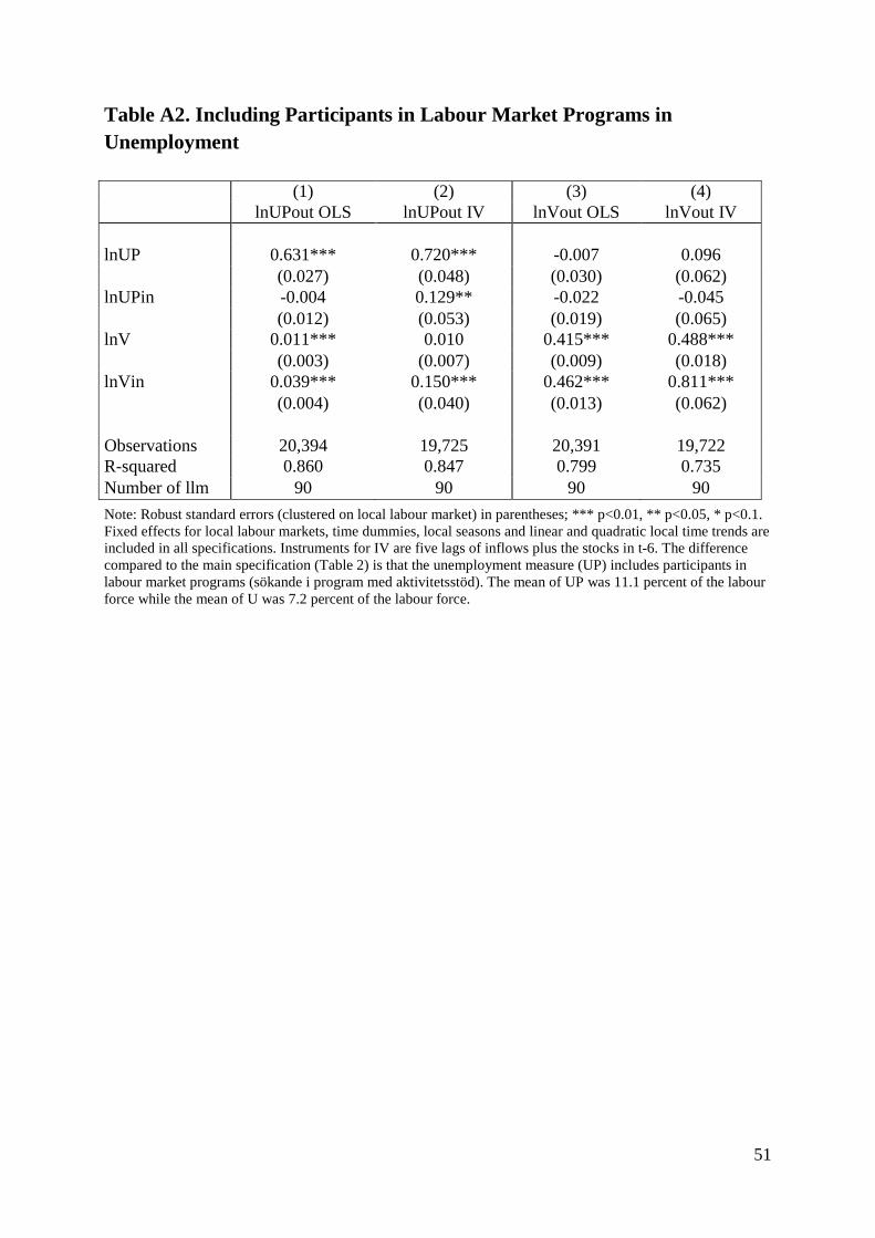
51
Table A2. Including Participants in Labour Market Programs in Unemployment
(1) (2) (3) (4) lnUPout OLS lnUPout IV lnVout OLS lnVout IV lnUP 0.631*** 0.720*** -0.007 0.096 (0.027) (0.048) (0.030) (0.062) lnUPin -0.004 0.129** -0.022 -0.045 (0.012) (0.053) (0.019) (0.065) lnV 0.011*** 0.010 0.415*** 0.488*** (0.003) (0.007) (0.009) (0.018) lnVin 0.039*** 0.150*** 0.462*** 0.811*** (0.004) (0.040) (0.013) (0.062) Observations 20,394 19,725 20,391 19,722 R-squared 0.860 0.847 0.799 0.735 Number of llm 90 90 90 90 Note: Robust standard errors (clustered on local labour market) in parentheses; *** p<0.01, ** p<0.05, * p<0.1. Fixed effects for local labour markets, time dummies, local seasons and linear and quadratic local time trends are included in all specifications. Instruments for IV are five lags of inflows plus the stocks in t-6. The difference compared to the main specification (Table 2) is that the unemployment measure (UP) includes participants in labour market programs (sökande i program med aktivitetsstöd). The mean of UP was 11.1 percent of the labour force while the mean of U was 7.2 percent of the labour force.

WORKING PAPERS* Editor: Nils Gottfries
2014:1 Oscar Erixson and Henry Ohlsson, Estate division: Equal sharing as choice, social norm, and legal requirement. 45 pp.
2014:2 Eva Mörk, Anna Sjögren and Helena Svaleryd, Parental unemployment and child health. 35 pp.
2014:3 Pedro Carneiro, Emanuela Galasso and Rita Ginja, Tackling Social Exclusion: Evidence from Chile. 87 pp.
2014:4 Mikael Elinder och Lovisa Persson, Property taxation, bounded rationality and housing prices. 38 pp.
2014:5 Daniel Waldenström, Swedish stock and bond returns, 1856–2012. 51 pp.
2014:6 Mikael Carlsson, Selection Effects in Producer-Price Setting. 34 pp.
2014:7 Ranjula Bali Swain and Fan Yang Wallentin, The impact of microfinance on factors empowering women: Differences in regional and delivery mechanisms in India’s SHG programme. 28 pp.
2014:8 Ashim Kumar Kar and Ranjula Bali Swain, Competition, performance and portfolio quality in microfinance markets. 33 pp.
2014:9 Shyam Ranganathan, Ranjula Bali Swain and David J.T. Sumpter, A DYNAMICAL SYSTEMS APPROACH TO MODELING HUMAN DEVELOPMENT. 42 pp.
2014:10 Shyam Ranganathan and Ranjula Bali Swain, Analysing Mechanisms for Meeting Global Emissions Target - A Dynamical Systems Approach. 40 pp.
2014:11 Chuan-Zhong Li and Ranjula Bali Swain, Growth, Water Resilience, and Sustainability: A DSGE Model Applied to South Africa. 21pp.
2015:1 Evelina Bonnier, Jonas Poulsen, Thorsten Rogall and Miri Stryjan, Preparing for Genocide: Community Work in Rwanda. 40 pp.
2015:2 Linna Martén, Political Bias in Court? Lay Judges and Asylum Appeals. 38 pp.
2015:3 Daniel Waldenström, The National Wealth of Sweden, 1810–2014. 31 pp.
2015:4 Daniel Waldenström, Wealth-income ratios in a small, late-industrializing, welfare-state economy: Sweden, 1810–2014. 41 pp.
2015:5 Mattias Nordin, Local Television, Citizen Knowledge and Political Accountability: Evidence from the U.S. Senate. 45 pp.
* A list of papers in this series from earlier years will be sent on request by the department.

2015:6 Glenn Mickelsson, Estimation of DSGE models: Maximum Likelihood vs.
Bayesian methods. 51 pp. 2016:1 Selva Bahar Baziki, Rita Ginja and Teodora Borota Milicevic. Trade
Competition, Technology and Labor Re-allocation. 83 pp. 2016:2 Matz Dahlberg, Kevin Mani, Mattias Öhman and Anders Wanhainen, Health
Information and Well-Being: Evidence from an Asymptomatic Disease. 32 pp.
2016:3 Federico Belotti, Edoardo Di Porto and Gianluca Santoni, The effect of local
taxes on firm performance: evidence from geo-referenced data. 37 pp. 2016:4 Edoardo Di Porto and Henry Ohlsson, Avoiding taxes by transfers within the
family. 35 pp. 2016:5 Eva Mörk and Mattias Nordin, Voting, Taxes and Heterogeneous
Preferences: Evidence from Swedish Local Elections. 30 pp. 2016:6 Luca Repetto, Political budget cycles with informed voters:
evidence from Italy. 46 pp. 2016:7 Spencer Bastani, Tomer Blumkin and Luca Micheletto, Anti-discrimination
Legislation and the Efficiency-Enhancing Role of Mandatory Parental Leave. 44 pp.
2016:8 Ylva Moberg, Does the gender composition in couples matter for the division
of labor after childbirth? 62 pp. 2016:9 Teodora Borota Milicevic and Mikael Carlsson, Markups from Inventory
Data and Export Intensity. 22 pp. 2016:10 Maria Björklund, Mikael Carlsson and Oskar Nordström Skans, Fixed Wage
Contracts and Monetary Non-Neutrality. 30 pp. 2016:11 Spencer Bastani, Ylva Moberg and Håkan Selin, The Anatomy of the
Extensive Margin Labor Supply Response. 50 pp 2016:12 Mikael Carlsson and Andreas Westermark, Endogenous Separations, Wage
Rigidities and Employment Volatility. 25 pp. 2016:13 Spencer Bastani and Jacob Lundberg, Political preferences for redistribution
in Sweden. 40 pp. 2016:14 Nils Gottfries and Karolina Stadin, The matching process: Search or
mismatch? 51 pp. See also working papers published by the Office of Labour Market Policy Evaluation http://www.ifau.se/ ISSN 1653-6975