Embed Size (px)
Citation preview

UNIVERSITA’ DEGLI STUDI DI BERGAMO DIPARTIMENTO DI INGEGNERIA GESTIONALE
QUADERNI DEL DIPARTIMENTO†
Department of Economics and Technology Management
Working Paper
n. 08 – 2007
Modelling and Testing for Structural Changes in Panel Cointegration Models with Common and Idiosyncratic Stochastic Trends
by
Chihwa Kao, Lorenzo Trapani and Giovanni Urga
† Il Dipartimento ottempera agli obblighi previsti dall’art. 1 del D.L.L. 31.8.1945, n. 660 e successive modificazioni.

COMITATO DI REDAZIONE§
Lucio Cassia, Gianmaria Martini, Stefano Paleari, Andrea Salanti § L’accesso alle Series è approvato dal Comitato di Redazione. I Working Papers ed i Technical Reports della Collana dei Quaderni del Dipartimento di Ingegneria Gestionale e dell’Informazione costituiscono un servizio atto a fornire la tempestiva divulgazione dei risultati dell’attività di ricerca, siano essi in forma provvisoria o definitiva.

Modelling and Testing for Structural Changes in Panel Cointegration Models with Common andIdiosyncratic Stochastic Trends�
Chihwa KaoSyracuse University
Lorenzo TrapaniCass Business School and Bergamo University
Giovanni UrgaCass Business [email protected]
March 7, 2007
Abstract
In this paper, we propose an estimation and testing framework for parameter instability in cointe-grated panel regressions with common and idiosyncratic trends. We develop tests for structural changefor the slope parameters under the null hypothesis of no structural break against the alternative hypoth-esis of (at least) one common change point which is possibly unknown. The limiting distributions of theproposed test statistics are derived. Monte Carlo simulations examine size and power of the proposedtests.
JEL classi�cation: C32; C33; C12; C13KEY WORDS: Panel cointegration; Common and idiosyncratic stochastic trends; testing for struc-
tural changes
�We are grateful for discussions with Robert De Jong, Long-Fei Lee, Zongwu Cai and Yupin Hu. We would also like to thankparticipants in the International Conferences on "Common Features in London" (Cass, 16-17 December 2004), 2006 New YorkEconometrics Camp and �Breaks and Persistence in Econometrics� (Cass, 11-12 December 2006), and econometrics seminarsat Ohio State University and Academia Sinica for helpful comments. Part of this work was done while Chihwa Kao was visitingthe Centre for Econometric Analysis at Cass (CEA@Cass). Financial support from City University 2005 Pump Priming Fundand CEA@Cass is gratefully acknowledged. Lorenzo Trapani acknowledges �nancial support from Cass Business School underthe RAE Development Fund scheme.
1 Introduction
Estimation and testing for structural changes is an important research topic in time series econometrics. A
recent annals volume of the Journal of Econometrics published in 2005 entitled �Modelling structural breaks,
long memory and stock market volatility�(edited by Anindya Banerjee and Giovanni Urga, 2005) and Perron
(2006) o¤er the most recent comprehensive reviews on the topic. In contrast, scarce is the literature on the
issues (estimation and testing) of structural changes in panel models, e.g., Han and Park (1989), Joseph
and Wolfson (1992, 1993), Joseph et al. (1997), Hansen (1999), Chiang et al. (2002), Emerson and Kao
(2001, 2002), Wachter and Tzavalis (2004) and Bai (2006). The estimation and testing for structure change
in panels have many applications in economics, For example, �scal/monetary policies may a¤ect every unit
in the economy (�rms/regions), stock market crashes in the US may also cause the chain reaction in other
stock markets in the world.
Despite the potential usefulness in economics, the econometric theory of the testing and estimation of
structural changes in panels is still underdeveloped. This paper �lls the gap in the literature by proposing an
estimation and testing framework for parameter instability in cointegrated panel regression. We derive tests
for structural change for the slope parameters in panel cointegration models with cross-sectional dependence
that is captured by the common stochastic trends. The tests are for the null hypothesis of no structural break
against the alternative hypothesis of (at least) one common change point which is possibly unknown. The
framework we propose is based on a linear cointegrated panel data model where the number of cross-sectional
units n and the number of time observations T are both large. The cointegrating equation we study contains
unit-speci�c variables (idiosyncratic shocks) and a set of possibly unobservable variables that are common
across all units (common shocks).
This paper makes two contributions to the existing literature. First, we develop an asymptotic theory
for the estimates of the parameters in the model. We consider both the case of observed and unobserved
common shocks. Ordinary large panels asymptotic theory (Phillips and Moon, 1999; Kao, 1999) cannot be
applied in our framework due to the strong cross-sectional dependence introduced by the common shocks.
We note that the limiting distributions of the common shocks coe¢ cients are mixed normal, in contrast with
asymptotic normality found in the literature. Second, along similar lines as Andrews (1993), we derive the
limiting distribution of a Wald-type test for the null hypothesis of no structural change at an unknown point
in cointegrated panels where units are cross dependent. The tests we derive are based on functionals of the
Wald-type statistic.
The organization of the paper is as follows. Section 2 introduces the model. Section 3 discusses asymp-
totics. The limiting distribution of the OLS under the null of no structural change is established. Section 4
de�nes the test statistic. The limiting distributions of the proposed test are also derived. Section 5 discusses
the local power. In Section 6 we report the �nite sample properties, i.e., size and power, of our proposed
1

tests. Section 7 provides concluding remarks. Some useful lemmas are given in Appendix A. In Appendix B
we report the proofs of the main results in the paper.
We write the integralR 10W (s)ds as
RW when there is no ambiguity over limits. We de�ne 1=2 to be any
matrix such that =�1=2
� �1=2
�0: We use k�k to denote the Euclidean norm of a vector, d�! to denote
convergence in distribution,p�! to denote convergence in probability, [x] to denote the largest integer � x,
I(0) and I(1) to signify a time-series that is integrated of order zero and one, respectively, B = BM () to
denote Brownian motion with the covariance matrix , and �B = B �RB to denote the demeaned version
of B: We let M <1 be a generic positive number which does not depend on n or T .
2 Model and Assumptions
Consider the following panel model with common and idiosyncratic shocks
yit = �i + �0Ft +
0xit + uit (1)
i = 1; :::; n and t = 1; :::; T; where �i is the individual e¤ect. The parameters � and are R � 1 and p� 1,
respectively, Ft = (F1t; :::; FRt)0 is a R� 1 vector of common stochastic trends
Ft = Ft�1 + "t (2)
xit is a p� 1 vector of observable I(1) individual-speci�c regressors,
xit = xit�1 + �it (3)
and�uit; "
0
t; �0
it
�0are error terms. When common shocks Ft are not observable in (1), we then assume that
Ft can be estimated by a set of observable exogenous variables, zit, such that
zit = �0iFt + eit (4)
where �i is a vector of factor loadings and eit is the error term.1
It is important to point out that our model in (1) is a standard common slope coe¢ cients panel model
not a factor-loading model as in Bai (2004), for example. Similar to this paper but not the same is Stock and
Watson (1999, 2002, 2005). In Stock and Watson�s setup, yit in (1) (with n = 1) is the time series variable
to be forecasted and zi = (zi1; zi2; :::; ziT )0 is a n-dimensional multiple time series of candidate predictors.
The main aim of this paper is to develop test statistics to test the constancy over time for � =��0; 0
�0with unknown change points. Considering the alternative hypothesis that there is only one change point k,
three possible sets of alternative hypotheses can be considered as opposed to the null of no structural change
1Kao, Trapani and Urga (2006) provide a comprehensive asymptotic theory of the OLS estimator � of � when (1) does notcontain idiosyncratic regressors xit.
2

in �: (1) only the common shocks coe¢ cients � may change, (2) only the idiosyncratic shocks coe¢ cients
may change or (3) both � and may be a¤ected by the break.
Denote �t =��0t;
0t
�0: Given the null hypothesis
H0 : �t = � for all t;
the alternative could be de�ned as
Ha : �t =
��1 for t = 1; :::; k�2 for t = k + 1; :::; T
with �1 6= �2.2
Note that testing for the constancy of � for the common factor, Ft, may have a di¤erent interpretation
than the usual constancy of the slope parameter.3 This is the case especially when Ft is not observed and
has to be estimated e.g. using the principal component estimator (see Bai, 2003, 2004; Bai and Ng, 2002,
2004). In this case, the estimated factor matrix, F , is given by T times the eigenvectors corresponding to the
R largest eigenvalues of the matrix ZZ 0, where Z = (z1; z2; :::; zn)0 is T �n with zi = (zi1; zi2; :::; ziT )0. Since
there is no guarantee that the R largest eigenvalues will have the same order for each t, the corresponding
eigenvectors will have di¤erent meanings over time. For example, in the term structure literature (see e.g.
Litterman and Scheinkman, 1991; Audrino et al. 2005), one usually uses a three-factor speci�cation (level,
slope and curvature) to explain the yield curves. The largest eigenvalue (and the corresponding eigenvector)
for period t may not the be the same one in period s. This will make the parameter � non constant. Thus,
� being non constant may indicate instability in the factor structure and not merely lack of constancy of a
slope parameter. Recently, Perignon and Villa (2006) provide some discussion on the stability of the latent
factor structure of interest rates over time.
We need the following assumptions.
Assumption M1: Let !it = (uit; "0t; �0it; eit)
0. We assume that
(a) !it is iid over t and the invariance principle holds for the partial sums of !it, so that for a given i,
1pT
bT �cXt=1
!itd�! B! (�) =
2664Bu (�)B" (�)B� (�)Be (�)
37752The formulation of the alternative hypothesis encompasses three possible cases:
Ha1 : �t=
�(�01;
0) for t = 1; :::; k(�02;
0) for t = k + 1; :::; T
Hb1: �t=
� ��0; 01
�for t = 1; :::; k�
�0; 02�
for t = k + 1; :::; T
Hc1: �t=
� ��01;
01
�for t = 1; :::; k�
�02; 02
�for t = k + 1; :::; T
where �1 6= �2 and 1 6= 2.3We thank Zongwu Cai for pointing this to us.
3

where B! (�) represents a multivariate Brownian motion, whose elements have covariance matrices �2u,
", � and e respectively.
(b) For a given t, fuitg, f"t; �itg ; and feitg are mutually independent across i.
(c) fxit; Ftg are not cointegrated and " and � are non singular.
(d) The eigenvalues of " and the random matrixRB"B
0" are distinct with probability 1.
Assumption M2: k�ik �M and 1n
Pni=1 �i�
0i ! �� as n!1, where �� is non singular.
Assumption M3: We assume the following limits hold as in Phillips and Moon (1999):
1
nT 2
nXi=1
TXt=1
exitex0it p�! 1
6� (5)
and1pnT
nXi=1
TXt=1
exituit d�! N
�0;1
6��
2u
�(6)
as (n; T ) �!1 where ~xit = xit � 1T
PTt=1 xit and �
2u = V ar (uit).
Assumption M1(a) considers a framework of no endogeneity of the regressors, serial dependence or con-
temporaneous correlation other than the one determined by the common shocks Ft are allowed for. Ex-
tensions to allow for endogeneity of the regressors, serial correlation and weak cross-sectional dependence
among the regression errors are straightforward. Assumption M1(a), therefore, is considered merely for the
purpose of simpli�cation. Assumption M1(b) is a standard requirement for factor analysis and it is needed
when Ft are not observable. Note here we allow non-zero covariance between "t and �it: Assumption M1(c)
rules out cointegration among regressors. Assumption M1(d) is a standard requirement in large panel factor
literature. Assumption M2 is also standard. Assumption M3 states that the joint limit theory developed by
Phillips and Moon (1999) holds for (5) and (6).
The following proposition is important for developing the asymptotics in this paper.
Proposition 1 Let Assumption M1 hold. As (n; T )!1
(a) 1pnT 2
Pni=1
PTt=1 wtex0it = Op (1),
(b) 1pnT
Pni=1
PTt=1 wtuit
d�! �u
�R�B" �B
0
"
�1=2� Z1
where Z1 � N (0; IR) and wt = Ft � 1T
PTt=1 Ft.
Proposition 1 states that the asymptotic magnitude of the cross termPni=1
PTt=1 wtex0it is Op �pnT 2�,
thereby smaller thanPni=1
PTt=1 exitex0it in (5) (and Pn
i=1
PTt=1 wtw
0t in (7) below). The asymptotic mixed
4

normality result in part (b) is also di¤erent from the distribution limit in equation (6) where asymptotic
normality holds. This result is due to the shock wt being common to all units and I(1).
We now turn to estimation of � (under the null of no structural change).
3 Asymptotics of the Parameter Estimates Under the Null
In this section we provide asymptotics for the OLS of model (1) under the null hypothesis of no structural
change. We distinguish the case of Ft observed from that where Ft needs to be estimated.
3.1 Ft is Observable
De�ne Wit = (w0t; ~x
0it)0. Let � be the OLS of �: Then we have
� � � =
�� � � �
�
=
"nXi=1
TXt=1
WitW0it
#�1 " nXi=1
TXt=1
Wituit
#
=
" Pni=1
PTt=1 wtw
0t
Pni=1
PTt=1 ~xitw
0tPn
i=1
PTt=1 wt~x
0it
Pni=1
PTt=1 ~xit~x
0it
#�1 " Pni=1
PTt=1 wtuitPn
i=1
PTt=1 ~xituit
#: (7)
The following proposition characterizes the limiting distribution of �.
Proposition 2 Let Assumptions M1(a)-M1(d) and M3 hold. Then, as (n; T ) �!1 it holds that
pnT�� � �
�=pnT
�� � � �
�d�! �u
�R�B" �B
0"
��1=2p6
�1=2�
!� Z (8)
where
Z � N��
00
�;
�IR 00 Ip
��:
Proposition 2 states that � � � and � are asymtotically independent. This result is a consequence of
Proposition 1, i.e.,
1
nT 2
" Pni=1
PTt=1 wtw
0t
Pni=1
PTt=1 ~xitw
0tPn
i=1
PTt=1 wt~x
0it
Pni=1
PTt=1 ~xit~x
0it
#=
24 Op (1) Op
�1pn
�Op
�1pn
�Op (1)
35 : (9)
Note that results in Proposition 2 havepnT convergence, as in Phillips and Moon (1999) and Kao
(1999). However, the limiting distribution of � is di¤erent from the panel cointegration literature, where
normality holds. The mixed normality found in our case is due to the shocks wt being nonstationary and
common across units, which implies 1nT 2
Pni=1
PTt=1 wtw
0t
d�!R�B" �B
0" being a random matrix rather than a
constant as in the standard panel cointegration as in (6).
5

3.2 Ft is Unobservable
In order to estimate � when Ft is unobservable, we consider a two step approach. First, we derive the
estimator of the vector of common shocks, Ft, using equation (4). We then plug this estimator in equation
(1) to retrieve an estimate for �.
3.2.1 Estimation of Ft
The estimator Ft, can be estimated by the method of principal components, (see e.g., Bai (2004)).4 That is,
Ft can be found by minimizing
VnT (R) =1
nT
nXi=1
TXt=1
�zit � �0iFt
�2subject to the normalization 1
T 2
PTt=1 FtF
0t = IR, where zit is given in (4). Let F = (F1; :::; FT )
0 and
Z = (z1; z2; :::; zn)0 a T � n matrix with zi = (zi1; zi2; :::; ziT )0. The estimator F =
�F1; :::; Ft
�0is a T � R
matrix which is found by T times the eigenvectors corresponding to the R largest eigenvalues of the T � T
matrix ZZ 0.
It is known that the solution to the above minimization problem is not unique, i.e., �i and Ft are not
directly identi�able since they are identi�able only up to a transformation. Therefore, instead of estimating
the factors Ft (or the loadings �i), what one does by employing the principal component estimator is to
estimate the space spanned by them up to a R � R transformation matrix, say H, thereby �nding HFt
instead of Ft. Therefore, computing the OLS of � for example, would result in estimating H�1� rather than
�. However, as far as testing is concerned, knowledge of HFt is the same as directly estimating Ft. Hence,
for the purpose of notational simplicity, we assume H being a R�R identity matrix in this paper.
3.2.2 Estimation of �
Let wt = Ft � 1T
PTt=1 Ft and Wit = (w
0t; ~x
0it)0. The OLS estimator of � is computed from
yit = �i + �0tFt +
0txit + vit (10)
where vit = uit + �0�Ft � Ft
�. Note
� � � =
�� � � �
�
=
"nXi=1
TXt=1
WitW0it
#�1 " nXi=1
TXt=1
Witvit
#
=
" Pni=1
PTt=1 wtw
0t
Pni=1
PTt=1 ~xitw
0tPn
i=1
PTt=1 wt~x
0it
Pni=1
PTt=1 ~xit~x
0it
#�1 " Pni=1
PTt=1 wtvitPn
i=1
PTt=1 ~xitvit
#: (11)
4Throughout the paper, we assume that the number of common shocks R is known. If this is not the case, detection of R ispossible using the methods derived by Bai and Ng (2002).
6

Let
�2� = �2u + �
2� (12)
where �2u = V ar(uit)
�2� = �0 ~QB
��2e��
�~Q0B� (13)
�2e = V ar(eit) and the random variable ~QB is de�ned as
1
T 2
TXt=1
wtw0t
d�! ~QB :
The following theorem characterizes the limiting distribution of � when Ft are not observable.
Theorem 1 Suppose Assumptions M1-M3 hold, with n=T ! 0 as (n; T )!1: We get
pnT�� � �
�=pnT
�� � � �
�d�! �R
�B" �B0"
��1=2��p
6�1=2� �u
!� Z (14)
where
Z � N��
00
�;
�IR 00 Ip
��:
Note that � and are asymptotically independent due to 1nT 2
Pni=1
PTt=1 WitW
0it being a block diagonal
matrix asymptotically similar to (9). The limiting distributions are essentially the same as those found in
Proposition 2, the only di¤erence with respect to (8), being the presence of the extra variance term �� in
the limiting distribution of �. This arises from the estimation error of the common shocks, Ft � Ft.
4 Test Statistics
The asymptotic theory for � derived in the Section 3 is used to derive the limiting distribution for the Wald-
type statistic under the null hypothesis of no structural change. A variety of tests for a break, based on the
Wald statistic have been discussed in the literature, e.g., Andrews (1993), Andrews and Ploberger (1994).
In this section, we consider three statistics: the supremum of the Wald statistic, SupW; the average Wald
statistic, AveW, and the logarithm of the Andrews-Ploberger exponential Wald statistic, ExpW.
Assumption PSE:(Partial Sample Estimation) kT ! r 2 (0; 1) as T and k !1:
Assumption PSE states that the fraction of T at which the change point occurs, r, is bounded away from
zero and one. Therefore, the structural break will divide the sample into two subsamples each of nontrivial
size. This assumption follows an argument similar to that in Corollary 1 in Andrews (1993, p.838).
Consider the following partial sample OLS
�1[Tr] =
0@ nXi=1
[Tr]Xt=1
WitW0
it
1A�1nXi=1
[Tr]Xt=1
Wityit
7
and
�2[Tr] =
0@ nXi=1
TXt=[Tr]+1
WitW0
it
1A�1nXi=1
TXt=[Tr]+1
Wityit:
Let �2u and �2� be consistent estimators for �
2u and �
2� respectively under H0. De�ne
��j[Tr] =
���IR 00 �uIp
��1�j[Tr]
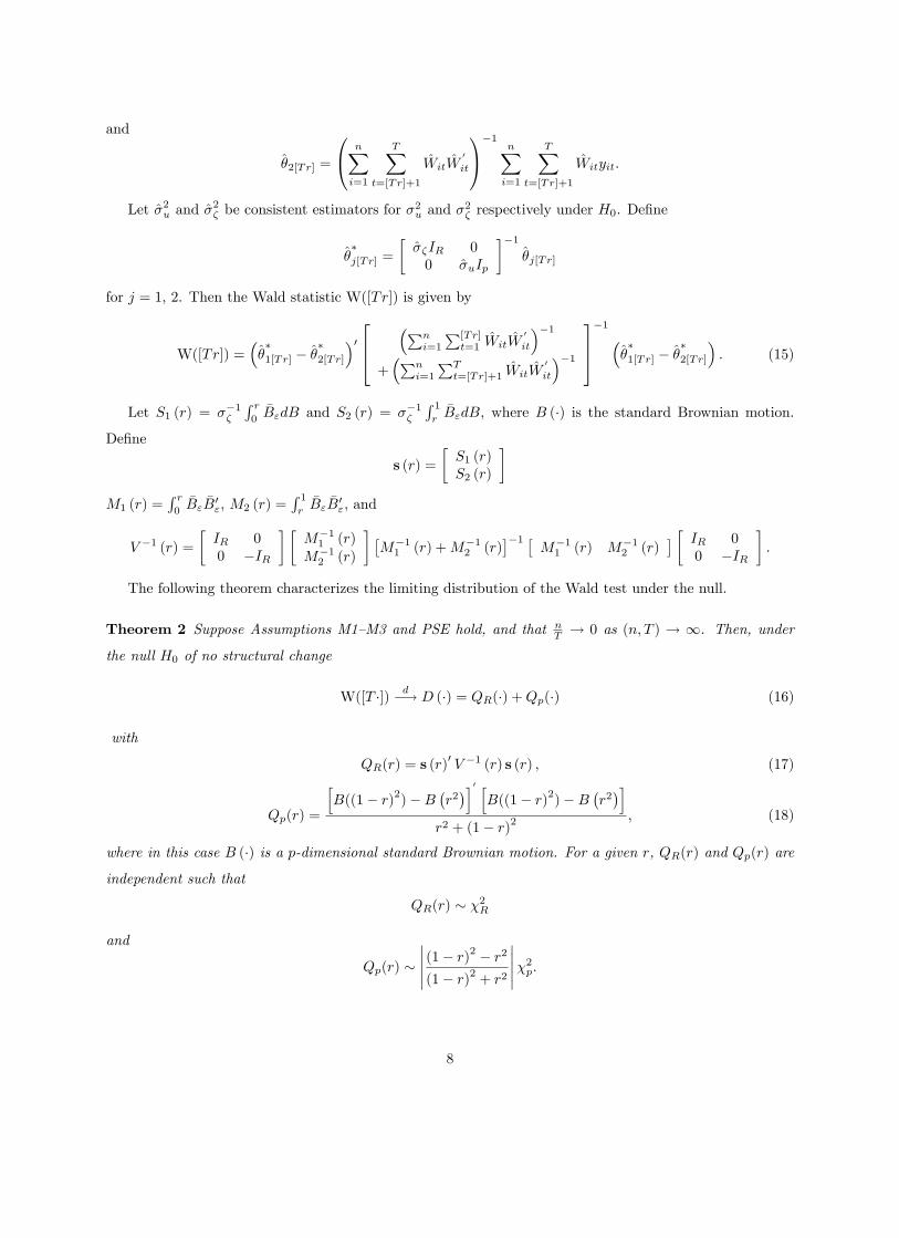
for j = 1, 2. Then the Wald statistic W([Tr]) is given by
W([Tr]) =���1[Tr] � �
�2[Tr]
�0 264�Pn
i=1
P[Tr]t=1 WitW
0
it
��1+�Pn
i=1
PTt=[Tr]+1 WitW
0
it
��1375�1 �
��1[Tr] � �
�2[Tr]
�: (15)
Let S1 (r) = ��1�R r0�B"dB and S2 (r) = ��1�
R 1r�B"dB, where B (�) is the standard Brownian motion.
De�ne
s (r) =
�S1 (r)S2 (r)
�M1 (r) =
R r0�B" �B
0", M2 (r) =
R 1r�B" �B
0", and
V �1 (r) =
�IR 00 �IR
� �M�11 (r)
M�12 (r)
� �M�11 (r) +M�1
2 (r)��1 �
M�11 (r) M�1
2 (r)� � IR 0
0 �IR
�:
The following theorem characterizes the limiting distribution of the Wald test under the null.
Theorem 2 Suppose Assumptions M1�M3 and PSE hold, and that nT ! 0 as (n; T ) ! 1. Then, under
the null H0 of no structural change
W([T �]) d�! D (�) = QR(�) +Qp(�) (16)
with
QR(r) = s (r)0V �1 (r) s (r) ; (17)
Qp(r) =
hB((1� r)2)�B
�r2�i0 h
B((1� r)2)�B�r2�i
r2 + (1� r)2; (18)
where in this case B (�) is a p-dimensional standard Brownian motion. For a given r, QR(r) and Qp(r) are
independent such that
QR(r) � �2R
and
Qp(r) ������ (1� r)2 � r2(1� r)2 + r2
������2p:
8

Let
d(r) =
����� (1� r)2 � r2(1� r)2 + r2
����� :Note that B((1� r)2)�B
�r2�has variance (1� r)2 � r2 if (1� r)2 > r2: Also B((1� r)2)�B
�r2�has
variance r2 � (1� r)2 if r2 > (1� r)2 : Then B((1� r)2)�B �r2� is a Bessel process of order p, andh
B((1� r)2)�B�r2�i0 h
B((1� r)2)�B�r2�i���(1� r)2 � r2���
is its standardized squares. Let s =���(1� r)2 � r2���, we can writeh
B((1� r)2)�B�r2�i0 h
B((1� r)2)�B�r2�i
r2 + (1� r)2=
s
r2 + (1� r)2BM(s)0BM(s)
s;
whereBM(s) denotes a p-vector of independent Brownian processes on [0;1]. For a �xed r, [BM(s)0BM(s)] =s
has a chi-squared distribution with p degrees of freedom. However, r cannot be 1=2 since s will be zero when
r = 1=2.
In order to obtain a test statistic that the critical values can be taken from the literature, e.g., Andrews
(1993), Andrews and Ploberger (1994), we consider the following modi�cation to the Wald test:
W�([Tr]) =����1[Tr] � �
��2[Tr]
�0 264�Pn
i=1
P[Tr]t=1 WitW
0
it
��1+�Pn
i=1
PTt=[Tr]+1 WitW
0
it
��1375�1 �
���1[Tr] � �
��2[Tr]
�
where
���j[Tr] =
���IR 0
0pd(r)� �uIp
��1�j[Tr]:
It is clear that
W�([T �]) d�! D� (�) = QR(�) +Q�p(�) (19)
where
Q�p(�) =1
d (r)Qp(�):
Note that for a �xed r, QR(r) and Q�p(r) are independent and
D� (r) � �2R+p:
Hence we have the following corollary:
Corollary 1 Suppose Assumptions M1�M3 and PSE hold, and that nT ! 0 as (n; T ) ! 1. Then, under
the null H0 of no structural change
W�([T �]) d�! D� (�)
9
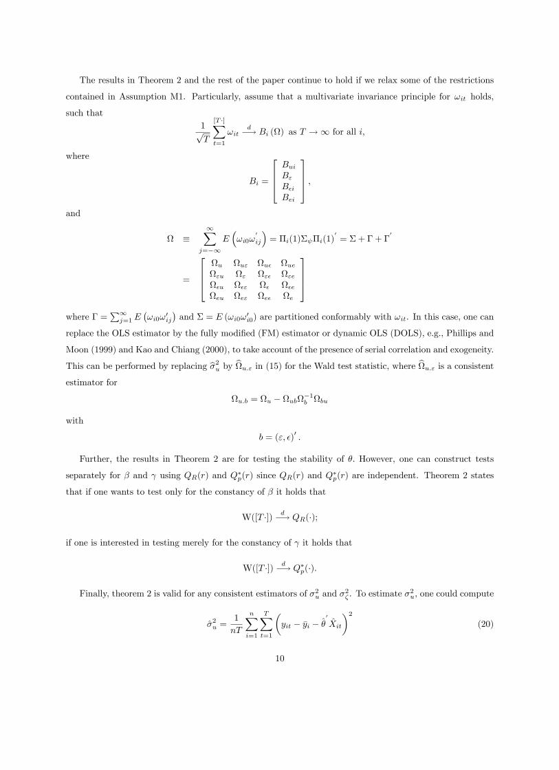
The results in Theorem 2 and the rest of the paper continue to hold if we relax some of the restrictions
contained in Assumption M1. Particularly, assume that a multivariate invariance principle for !it holds,
such that1pT
[T �]Xt=1
!itd�! Bi () as T !1 for all i;
where
Bi =
2664BuiB"B�iBei
3775 ;and
�1X
j=�1E�!i0!
0
ij
�= �i(1)� �i(1)
0= �+ � + �
0
=
2664u u" u� ue"u " "� "e�u �" � �eeu e" e� e
3775where � =
P1j=1E
�!i0!
0ij
�and � = E (!i0!0i0) are partitioned conformably with !it. In this case, one can
replace the OLS estimator by the fully modi�ed (FM) estimator or dynamic OLS (DOLS), e.g., Phillips and
Moon (1999) and Kao and Chiang (2000), to take account of the presence of serial correlation and exogeneity.
This can be performed by replacing b�2u by bu:" in (15) for the Wald test statistic, where bu:" is a consistentestimator for
u:b = u � ub�1b bu
with
b = ("; �)0:
Further, the results in Theorem 2 are for testing the stability of �: However, one can construct tests
separately for � and using QR(r) and Q�p(r) since QR(r) and Q�p(r) are independent. Theorem 2 states
that if one wants to test only for the constancy of � it holds that
W([T �]) d�! QR(�);
if one is interested in testing merely for the constancy of it holds that
W([T �]) d�! Q�p(�):
Finally, theorem 2 is valid for any consistent estimators of �2u and �2� . To estimate �
2u, one could compute
�2u =1
nT
nXi=1
TXt=1
�yit � �yi � �
0
Xit
�2(20)
10

which is consistent under H0. To �nd a consistent estimator, �2� , of �
2� , from equation (12) a possible choice
is
�2� = �2u + �
2�:
From equation (13), we have
�2� = �0�2��;
with
�2� =
1
T 2
TXt=1
wtw0t
!"1
n
nXi=1
1
T
TXt=1
e2it
!�i�
0i
# 1
T 2
TXt=1
wtw0t
!; (21)
where �i is a consistent estimate of �i and eit can be computed as
eit = zit � �0iFt:
Therefore, we can provide an estimate for �2� as
�2� = �2u + �
0�2��: (22)
The following proposition characterizes the consistency of �2u and �2� under H0.
Proposition 3 Suppose Assumptions M1-M3 hold and that nT ! 0 as (n; T )!1. Then, under H0
�2up�! �2u;
�2�p�! �2� :
The limiting distribution for the Wald test is now used to test for the presence of a structural break.
Following Andrews (1993) and Andrews and Ploberger (1994), we consider three functionals of the Wald
statistic W(�):
SupW(k) = sup[Tr�]�k�T�[Tr�]
W�(k);
AveW(k) =1
T
T�[Tr�]Xk=[Tr�]
W�(k);
and
ExpW(k) = log
8<: 1TT�[Tr�]Xk=[Tr�]
exp
�1
2W�(k)
�9=;where r� represents the fraction of the sample trimmed away from the beginning and the end of the sam-
ple. Therefore, to carry out the test we only use data belonging to the sub-interval of the full sample
f[Tr�] ; [Tr�] + 1; :::; T � [Tr�]� 1; T � [Tr�]g. Using the continuous mapping theorem (CMT) we have the
following result:
11

Corollary 2 Suppose Assumptions M1-M3 and PSE hold; then under H0:
SupW([Tr])d�! sup
r��r�1�r�D�(r);
AveW([Tr])d�!R 1�r�r�
D�(r)dr;
ExpW([Tr])d�! log
nR 1�r�r�
exp�12D
�(r)�dro
as (n; T )!1:
Critical values for SupW; AveW; and ExpW can be taken from Andrews (1993) and Andrews and
Ploberger (1994) since D� (r) is �2R+p for a �xed r. For example, when r� = 0:15 and R = p = 1; the critical
values of the 5% level for SupW; AveW; and ExpW are 11:79, 4:61, and 3:22 respectively.
5 Local Asymptotic Power
In this section, we evaluate the power of the Wald statistic against local alternatives. We assume the following
sequence of local alternatives:
H(nT )a : �
(nT )t = � +
1pnTg
�t
T
�(23)
where g (�) =hg0� (�) ; g0 (�)
i0is a (R+ p) � 1 arbitrary function de�ned on the unit interval, with the sub-
elements g� (�) and g (�) being R� 1 and p� 1 respectively.
The properties of g�tT
�are speci�ed in the following assumption.
Assumption LP:(Local Power) The function g�tT
�belongs to the class of Riemann integrable functions
and as (n; T )!1 and for all k:
(a) 1T
P[Tr]t=1 g
�tT
�!R r0g(s)ds;
(b) 1nT 2
Pni=1
P[Tr]t=1 WitW
0itg�tT
�= Op (1),
(c) 1nT 2
Pni=1
P[Tr]t=1
1pTW 0itg�tT
�= Op (1),
(d) 1nT 2
Pni=1
P[Tr]t=1 g
0 � tT
�WitW
0itg�tT
�= Op (1),
(e) 1nT
Pni=1
P[Tr]t=1 W
0itg�tT
�uit = Op (1).
Possible alternative functional forms for g (�) include: the constant function, i.e. g (�) = c over the whole
sample, which indicates no structural breaks; a single step function, i.e., g (s) = 0 if r < r and g (s) = 4� if
s � r, which represents a one-time change on � at k = [Tr]; multiple steps functions that represent multiple
changes; time trending function g (�) = t=T .
Assumptions LP(b)-(e) are technical requirements needed in order for g (�) to be a non-trivial local
alternative, i.e., in order for g (�) not to vanish too quickly as T !1.
12

In what follows, we derive the asymptotic behavior of the Wald statistic under the sequence of local
alternatives (23). Model (1) can be rewritten as
y(nT )it = �i +X
0it�
(nT )t + uit:
Similarly, when common shocks are replaced by their estimates Xit we have
y(nT )it = �i + X
0it�
(nT )t + vit
with vit = uit +�Ft � Ft
�0�(nT )t . Let �
(nT )
1k and �(nT )
2k be the OLS estimators under the local alternative
(23), and let ~�2u and ~�2� be consistent estimators for �
2u and �
2� respectively under the local alternatives
H(nT )a . De�ne
��(nT )jk =
�~��IR 00 ~�uIp
��1�(nT )
jk ;
for j = 1; 2, the Wald statistics under the local alternative can be computed as
W (nT )(k) =h��(nT )1k � �
�(nT )2k
i0 264�Pn
i=1
Pkt=1 WitW
0
it
��1+�Pn
i=1
PTt=k+1 WitW
0
it
��1375�1 h
��(nT )1k � �
�(nT )2k
i: (24)
The local asymptotic power for the Wald statistics is given in the following theorem.
Theorem 3 Suppose Assumptions M1-M3, PSE and LP hold. Then under the local alternative hypotheses
H(nT )a de�ned in equation (23),
W (nT )([T �]) d�! D (�) +Op (1)
where D (r) is de�ned in Theorem 2.
The arguments in Theorem 3 also hold for the modi�ed Wald test statistic. Theorem 3 indicates that the
Wald statistics in (24) has nontrivial local power irrespective of the particular type of the structural change.
The theorem holds for any choice of the estimators ~�2u and ~�2� which is consistent under H
(nT )a . A possible
estimator for �2u is
~�2u =1
nT
nXi=1
TXt=1
hyit � �yi � �
(nT )0t Xit
i2:
To estimate �2� we propose
~�2� = ~�2u + �
(nT )0�2��
(nT );
where �2� is de�ned in equation (21) and �(nT )
is the OLS estimator for � under H(nT )a . Then the following
proposition establishes consistency for ~�2u and ~�2� under H
(nT )a .
Proposition 4 Suppose Assumptions M1-M3, PSE and LP hold. Then under the local alternative hypothe-
ses H(nT )a de�ned in equation (23), it holds that
~�2up�! �2u;
13

~�2�p�! �2�
as (n; T )!1
6 Monte Carlo Simulations
In this section we present the simulation results that are designed to assess the null rejection probabilities
and the power properties of SupW(k); AveW(k); and ExpW(k) statistics. To compare the performance of
the proposed tests we conduct Monte Carlo experiments based on the following design
yit = �i + �0tFt +
0txit + uit
Ft = Ft�1 + "t;
xit = xit�1 + �it;
and
zit = �0iFt + eit
for i = 1; :::; n; t = 1; :::; T; where the vector [uit; "0it; �0it; e
0it] is randomly drawn from a standard multivariate
normal distribution.
For this experiment, we assume a single factor, i.e., R = 1 and �i is generated from i.i.d. N(��; 1). We
set �� = 2. Under the null hypothesis of no structural change, we set the values of the parameters � = 1
and = 1. Also we choose �i � N(0; 1).
We assess the power of the test considering an alternative hypothesis of structural change in both � and
. We consider break location is assumed to take place at the 40% of the sample. To control for the break
magnitude, we simulate model (1)-(4) assuming that, under Ha
�t =
�� for t < k(1 + c) � for t � k
where c is a scalar that de�nes the percentage change in the parameter values. We set c = 0:1. When
generating the DGP, the �rst 1,000 observations are discarded to avoid dependence on the initial conditions.
All our results are based on sample size of n = f20; 40; 60; 120; 240; 480g and T = f20; 40; 60; 120; 240; 480g
with 10,000 iterations. The size and power are evaluated at 5% level. All programs are written by GAUSS.
The the critical values of the 5% level for SupW; AveW; and ExpW are 11:79, 4:61, and 3:22 respectively.
Those critical values were taken from Andrews (1993) and Andrews and Ploberger (1994).
Table 1 contains empirical rejection frequencies of the test statistics, SupW; AveW; and ExpW, under
the null that � and are stable over time. It is clear from Table 1 that all these three test statistics are
undersized if n and T are small. Overall, all three test statistics show good size when n and T are large.
14

Table 2 gives the power of the test statistics. All tests show very good power properties. The power gain
is substantial as T increases and more moderate for increasing sizes of n. This result is consistent with thepnT asymptotics of the three tests, as reported in the paper.
7 Conclusion
In this paper, we derive an asymptotic theory for testing for an unknown common change point in a coin-
tegrated panel regression with common and idiosyncratic shocks. We develop the asymptotic theory for the
cases of observable and unobservable common shocks and we derive the limiting distribution of the supre-
mum, average and exponential Wald-type statistics under the null of no structural change. The derived
limiting distributions are nuisance parameter free, depending only on the number of regressors. Monte Carlo
simulations show that all three tests have good size and power properties, the power gain being substantial
as T increases and more moderate for increasing sizes of n, consistent with thepnT asymptotics of the three
tests.
15

Appendix
De�ne CnT = min fpn; Tg, wt =
�Ft � �F 0
�, �F 0 = T�1
PTt=1 Ft, bwt = ( bFt � �F ), and �F = 1
T
PTt=1
bFt:A Lemmas
Lemma A.1 Under Assumptions M1 and M2, as (n; T )!1
(a) 1T
PTt=1
Ft � Ft 2 = Op �C�2nT �,(b) 1
T
PTt=1 kwt � wtk
2= Op
�1
C2nT
�,
(c) 1T
PTt=1 w
0t
�Ft � Ft
�= Op
�1
CnT
�.
Proof. Part (a) is taken from Lemma 1 in Bai (2004). Consider part (b).
1
T
TXt=1
kwt � wtk2 =1
T
TXt=1
�Ft � Ft�+ � �F � �F 0� 2
� 2
T
TXt=1
� Ft � Ft 2 + �F � �F 0 2� = I + II:
Now, I = T�1PTt=1
Ft � Ft 2 = Op �C�2nT � from part (a).. For II, it holds that
�F � �F 0 2 = 1T
TXt=1
�Ft � Ft
� 2
� 1
T
TXt=1
Ft � Ft 2! = Op� 1
C2nT
�;
using the Cauchy-Schwartz inequality. Therefore 1T
PTt=1
�F � �F 0 2 = Op � 1
C2nT
�, and consequently
1
T
TXt=1
kwt � wtk2 = Op�
1
C2nT
�:
This proves (b). Part (c) follows directly from Lemma B.4(i) in Bai (2004).
Lemma A.2 Under Assumptions M1 and M2, as (n; T ) �!1
(a)1
T 2
TXt=1
wtw0
t =1
T 2
TXt=1
wtw0t +Op
�1pTCnT
�with
1
T 2
TXt=1
wtw0t = Op (1) ;
16

(b)1pnT
nXi=1
TXt=1
wtuit =1pnT
nXi=1
TXt=1
wtuit +Op
�1
CnT
�with
1pnT
nXi=1
TXt=1
wtuit = Op (1) ;
(c)1pnT
nXi=1
TXt=1
wt
�Ft � Ft
�=
1pnT
nXi=1
TXt=1
w0t
�Ft � Ft
�+Op
� pn
C2nT
�with
1pnT
nXi=1
TXt=1
w0t
�Ft � Ft
�= Op
� pn
CnT
�:
Proof. For part (a), note that
1
T 2
TXt=1
wtw0t =
1
T 2
TXt=1
(wt + wt � wt) (wt + wt � wt)0
=1
T 2
TXt=1
wtw0t +
1
T 2
TXt=1
wt (wt � wt)0
+1
T 2
TXt=1
(wt � wt)w0t +1
T 2
TXt=1
(wt � wt) (wt � wt)0
= I + II + III + IV:
Assumption M1 ensures that
I = Op (1) :
As far as terms II and III are concerned, application of the Cauchy-Schwartz inequality and of Lemma
A.1(a) ensures that they are bounded by
II � 1
T 2
TXt=1
kwtk2!1=2 TX
t=1
kwt � wtk2!1=2
=1
T 2Op (T )Op
pT
CnT
!= Op
�1pTCnT
�:
Use Lemma A.1(a) we have 1T 2TXt=1
(wt � wt) (wt � wt)0 � 1
T 2
TXt=1
kwt � wtk2 = Op�
1
TC2nT
�:
Hence,
1
T 2
TXt=1
wtw0t =
1
T 2
TXt=1
wtw0t +Op
�1pTCnT
�+Op
�1
TC2nT
�:
17
For part (b), note that
1pnT
nXi=1
TXt=1
wtuit =1pnT
nXi=1
TXt=1
wtuit +1pnT
nXi=1
TXt=1
(wt � wt)uit = I + II:
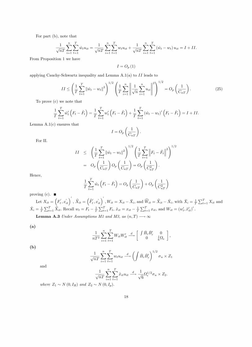
From Proposition 1 we have
I = Op (1)
applying Cauchy-Schwartz inequality and Lemma A.1(a) to II leads to
II � 1
T
TXt=1
kwt � wtk2!1=20@ 1
T
nXi=1
1pn
nXi=1
uit
21A1=2
= Op
�1
CnT
�: (25)
To prove (c) we note that
1
T
TXt=1
w0t
�Ft � ~Ft
�=1
T
TXt=1
w0t
�Ft � ~Ft
�+1
T
TXt=1
(wt � wt)0�Ft � Ft
�= I + II:
Lemma A.1(c) ensures that
I = Op
�1
CnT
�:
For II.
II � 1
T
TXt=1
kwt � wtk2!1=2
1
T
TXt=1
Ft � Ft 2!1=2
= Op
�1
CnT
�Op
�1
CnT
�= Op
�1
C2nT
�:
Hence,
1
T
TXt=1
wt
�Ft � Ft
�= Op
�1
CnT
�+Op
�1
C2nT
�proving (c).
Let Xit =�F
0
t ; x0
it
�0; bXit = � bF 0
t ; x0
it
�0;Wit = Xit � �Xi; and cWit = bXit � Xi, with �Xi =
1T
PTt=1Xit and
Xi =1T
PTt=1
bXit: Recall wt = Ft � 1T
PTt=1 Ft, ~xit = xit � 1
T
PTt=1 xit, and Wit = (w
0t; ~x
0it)0:
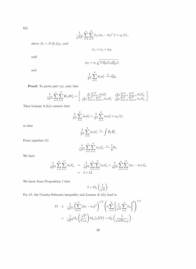
Lemma A.3 Under Assumptions M1 and M3, as (n; T ) �!1
(a)1
nT 2
nXi=1
TXt=1
WitW0it
d�!� R
�B" �B0" 0
0 16�
�;
(b)1pnT
nXi=1
TXt=1
wtuitd�!�Z
�B" �B0"
�1=2�u � Z1
and1pnT
nXi=1
TXt=1
~xituitd�! 1p
61=2� �u � Z2:
where Z1 � N (0; IR) and Z2 � N (0; Ip).
18

Proof. To prove (a), note
1
nT 2
nXi=1
TXt=1
WitW0it =
"1T 2
PTt=1 wtw
0t
1nT 2
Pni=1
PTt=1 wt~x
0it
1nT 2
Pni=1
PTt=1 ~xitw
0t
1nT 2
Pni=1
PTt=1 ~xit~x
0it
#
=
�a bb0 c
�:
Assumption M1(a) ensures that
a =1
T 2
TXt=1
wtw0t
d�!Z�B" �B
0";
Equation (5) in Assumption M3 states that
c =1
nT 2
nXi=1
TXt=1
~xit~x0it
p�! 1
6�2u�;
We know from Proposition 1 that
1
nT 2
nXi=1
TXt=1
~xitw0t = op (1) :
In order to prove (b), note that
1pnT
nXi=1
TXt=1
Wituit =
"1pnT
Pni=1
PTt=1 wtuit
1pnT
Pni=1
PTt=1 ~xituit
#
=
�cd
�:
From equation (6) in Assumption M3 that
1pnT
nXi=1
TXt=1
~xituitd�! N
�0;1
6��
2u
�=
1p61=2� �u � Z2
We also know from Proposition 1
1pnT
nXi=1
TXt=1
wtuitd�!�Z
�B" �B0"
�1=2�u � Z1:
This proves part (b).
Lemma A.4 Under Assumptions M1-M3 it holds that, as (n; T ) �!1 andpnT �! 0
(a)1
nT 2
TXt=1
WitW0it
d�!� R
�B" �B0" 0
0 16�
�;
(b)1pnT
nXi=1
TXt=1
wt�uit + �
0 (wt � wt)� d�!
�Z�B" �B
0"
�1=2�� � Z1;
19
(c)1pnT
nXi=1
TXt=1
~xit (wt � wt)0 � = op (1) ;
where Z1 � N (0; IR), and
�� = �u + ��;
with
�� = �e
q�0 ~QB�� ~Q0B�;
and1
T 2
TXt=1
wtw0t
d�! ~QB :
Proof. To prove part (a), note that
1
nT 2
nXi=1
TXt=1
WitW0it =
"1T 2
PTt=1 wtw
0t
1nT 2
Pni=1
PTt=1 wt~x
0it
1nT 2
Pni=1
PTt=1 ~xitw
0t
1nT 2
Pni=1
PTt=1 ~xit~x
0it
#:
Then Lemma A.2(a) ensures that
1
T 2
TXt=1
wtw0t =
1
T 2
TXt=1
wtw0t + op (1) ;
so that1
T 2
TXt=1
wtw0t
d�!Z�B" �B
0":
From equation (5)
1
nT 2
nXi=1
TXt=1
~xit~x0it
p�! 1
6�:
We have
1
nT 2
nXi=1
TXt=1
wt~x0it =
1
nT 2
nXi=1
TXt=1
wt~x0it +
1
nT 2
nXi=1
TXt=1
(wt � wt) ~x0it
= I + II:
We know from Proposition 1 that
I = Op
�1pn
�:
For II, the Cauchy-Schwartz inequality and Lemma A.1(b) lead to
II � 1
nT 2
TXt=1
kwt � wtk2!1=20@n TX
t=1
1pn
nXi=1
~xit
21A1=2
=1
nT 2Op
pT
CnT
!Op�pnT�= Op
�1p
nTCnT
�:
20

Therefore, as (n; T ) �!11
nT 2
nXi=1
TXt=1
wt~x0it = op (1) :
To prove part (b), note that
1pnT
nXi=1
TXt=1
wt�uit + �
0 (wt � wt)�=
1pnT
nXi=1
TXt=1
wtuit +1pnT
nXi=1
TXt=1
wt (wt � wt)0 �
= a+ b:
As far as a is concerned, we have
a =1pnT
nXi=1
TXt=1
wtuit +1pnT
nXi=1
TXt=1
(wt � wt)uit
= I + II;
and according to Lemma A.3(b) we have
Id�!�Z
�B" �B0"
�1=2�u � Z1:
For II, we have
II � 1pnT
TXt=1
kwt � wtk2!1=20@n TX
t=1
1pn
nXi=1
uit
21A1=2
=1pnTOp
pT
CnT
!Op
�pnT�= Op
�1
CnT
�:
Therefore, II = op (1) and
a =1pnT
nXi=1
TXt=1
wtuit + op (1) :
For b, we know from Bai (2004) that, as (n; T ) �!1 andpnT �! 0 we have
pn (wt � wt) =
1
T 2
TXs=1
wsw0s
1pn
nXi=1
�ieit = Op (1) :
Therefore we write
b =1pnT
nXi=1
TXt=1
wt (wt � wt)0 � +1pnT
nXi=1
TXt=1
(wt � wt) (wt � wt)0 �
=1pnT
nXi=1
TXt=1
wt (wt � wt)0 � + op (1) :
Hence
1pnT
nXi=1
TXt=1
wt�uit + �
0 (wt � wt)�
=1pnT
nXi=1
TXt=1
wt�uit + (wt � wt)0 �
�+ op (1) :
21

From Theorem 2 in Bai (2004) we know that for a given t
pn (wt � wt) =
bw0w
T 2
!1pn
nXi=1
�ieit + op (1)d�! eQBN (0;�)
as n �!1 where bw0w
T 2d�! eQB ;
and
� = limn!1
1
n
nXi=1
nXj=1
E��i�
0
jeitejt
�= �2e lim
n!1
1
n
nXi=1
nXj=1
�i�0
j
= �2e��:
Then
1
T
TXt=1
wt�0pn (wt � wt) =
1
T
TXt=1
wt�0 eQBN (0;�) + op (1)
=1
T
TXt=1
wt�t + op (1)
where
�t = �0 eQBN (0;�) :
It is clear that1
T
TXt=1
wt�td�!Z�B0
"dB�
as T !1 where B� is de�ned as1pT
tXj=1
�jd�! B� = ��B
�: (26)
where B� is the standard Brownian motion. It follows that
1
T
TXt=1
wt�0pn (wt � bwt) d�!
Z�B0
"dB� =
�Z�B" �B
0
"
�1=2�� � Z1
Finally, consider the joint distribution of the elements in"1pnT
Pni=1
PTt=1 bwtuit
1pnT
Pni=1
PTt=1 bwt�0 (wt � bwt)
#: (27)
Any linear combination of these elements takes the form
1pn
nXi=1
(1
T
TXt=1
h�1 bwtuit + �2 bwt�0 (wt � bwt)i
)
22
for some �1 and �2: Let
&iT =1
T
TXt=1
h�1 bwtuit + �2 bwt�0 (wt � bwt)i :
For a given T , it is also clear that every element of &iT are iid across i conditional on C, the �-algebra
generated by fFtg. Without loss of the generality, we assume R = 1. It is clear that every element of &iTare iid across i conditional on C which is an invariant �-�eld. Thus
1
n
nXi=1
&iT &0
iTp�! E
�&iT &
0
iT jC�
where
E�&iT &
0
iT jC�
= var
"1
T
TXt=1
bwt h�1uit + �2�0 (wt � bwt)i#
=1
T 2
TXt=1
V arnbwt h�1uit + �2�0 (wt � bwt)io
=1
T 2
TXt=1
nbwt bw0
t
h�21var (uit) + 2�1�2E
huit�
0(wt � bwt)i+ �22var�0 ((wt � bwt))io
and
1
n
nXi=1
1
T 2
TXt=1
nbwt bw0
t
h�21var (uit) + 2�1�2E
huit�
0(wt � bwt)i+ �22var�0 (wt � bwt)io
=1
n
nXi=1
1
T 2
TXt=1
bwt bw0
t�21var (uit) + 2
1
n
nXi=1
1
T 2
TXt=1
bwt bw0
t2�1�2Ehuit�
0(wt � bwt)i
+1
n
nXi=1
1
T 2
TXt=1
bwt bw0
t�22var�
0(wt � bwt) :
23

Notice that E and var are conditional expectation and conditional variance respectively. It follows that
conditional on C, 1nnXi=1
1
T 2
TXt=1
bwt bw0
t2�1�2Ehuit�
0(wt � bwt)i
=
1nnXi=1
1
T 2
TXt=1
bwt bw0
t2�1�2Ehuit�
0(wt � bwt)i
=
1
T 2pn
TXt=1
bwt bw0
t2�1�2E
""1pn
nXi=1
uit
#�0(wt � bwt)#
=
1
T 2pn
TXt=1
bwt bw0
t2�1�2Ehut�
0(wt � bwt)i
� 1p
n2 k�1�2k
1
T 2
TXt=1
bw2t 2!1=2
E1
T 2
TXt=1
ut�0 (wt � bwt) 2!1=2= op (1)
with
ut =1pn
nXi=1
uit
since
E1
T 2
TXt=1
ut�0 (wt � bwt) 2 = op (1)and
1
T 2
TXt=1
bw2t 2 = Op (1) :Also
1
T 2
TXt=1
bwt bw0
t�21var (uit)
d�!Z�B" �B
0
"�21�
2u
and1
T 2
TXt=1
bwt bw0
t�22var�
0(wt � bwt) d�!
Z�B" �B
0
"�22�
2�:
Let Ii be the � �eld generated by Ft and (&1T ; :::; &iT ). Then f&iT ; Iig is a martingale di¤erence sequence
(MDS) with positive variance given by E�&iT &
0
iT jC�satisfying
E�&iT &
0
iT jC�
p�!ZB"B
0
"
��21�
2u + �
22�
2�
�=
�Z�B" �B
0
"
��0�
with � = (�1; �2)0where
=
��2u 00 �2�
�:
24

Hence, we can use the MDS CLT to get
1pn
nXi=1
&iTd�!hE�&iT &
0
iT jC�i1=2
� Z =��Z
�B" �B0
"
��0�
�1=2� Z + op (1)
where Z � N (0; IR) and E��i�
0ijC�and Z are independent. Thus, any linear combination of the two
elements in the vector in (27) is asymptotically mixed normal, i.e.,"1pnT
Pni=1
PTt=1 bwtuit
1pnT
Pni=1
PTt=1 bwt�0 �Ft � bFt�
#d�!�Z
�B" �B0
"
�1=2� Z
with
=
��2u 00 �2�
�and Z and
R�B" �B
0
" are independent. Then
1pnT
nXi=1
TXt=1
wt�uit + �
0 (wt � wt)�
=1pnT
nXi=1
TXt=1
bwtuit + 1pnT
nXi=1
TXt=1
bwt�0 (wt � bwt)d�!�Z
�B" �B0
"
��1�Z�B" �B
0
"
�1=2 �1 1
�1=2 � Z
=
�Z�B" �B
0
"
��1=2�� � Z
with
�� = �u + ��:
This proves (ii).
Consider (iii). Recall that we have, as (n; T )!1 withpnT ! 0
1pnT
nXi=1
TXt=1
~xit (wt � wt)0 �
=1
nT
nXi=1
TXt=1
~xit
24 1T 2
TXs=1
wsw0s
!0@ 1pn
nXj=1
�jejt
1A350 � + op (1)=
1pnT
24 TXt=1
1pn
nXi=1
~xit
!0@ 1pn
nXj=1
ejt�0j
1A35 1
T 2
TXs=1
wsw0s
!0� + op (1) :
As T !1, and for all n, we have
TXt=1
1pn
nXi=1
~xit
!0@ 1pn
nXj=1
ejt�0j
1A = Op (T ) ;
25

therefore, for (n; T )!1 we have
1pnT
TXt=1
1pn
nXi=1
~xit
!�0
1
T 2
TXs=1
wsw0s
!0@ 1pn
nXj=1
�jejt
1A = Op
�1pn
�:
This proves the Lemma.
Lemma A.5 Let Assumptions M1-M3 and PSE hold. Then, as (n; T ) ! 1 withpn=T ! 0, it holds
that
(a)1
nT 2
nXi=1
kXt=1
WitW0it
d�!� R r
0�B" �B
0" 0
0 16r2�
�;
1
nT 2
nXi=1
TXt=k+1
WitW0it
d�!" R 1
r�B" �B
0" 0
0 16 (1� r)
2�
#;
(b)1pnT
nXi=1
kXt=1
Wit
�uit + �
0 (wt � wt)� d�!
" �R r0�B" �B
0"
�1=2�� � Z1
1p6r�u
1=2� � Z2
#;
1pnT
nXi=1
TXt=k+1
Wit
�uit + �
0 (wt � wt)� d�!
24 �R 1r�B" �B
0"
�1=2�� � Z1
1p6(1� r)�u1=2� � Z2
35 ;for all r where Z1 and Z1 are independent standard normals of dimensions R and p respectively.
Proof. The results are taken directly from Lemma A.4 and Chiang et al. (2002).
B PROOFS
B.1 Proof of Proposition 1
Proof. Consider (a). Note
1pnT
nXi=1
TXt=1
wtex0it=
1
T
TXt=1
wt
1pn
nXi=1
ex0it!
= Op (1) :
This is because5
1pn
nXi=1
ex0it � I(1)5Let�s assume p = 1 and �2� = 1
xit = xit�1 + �it =tX
j=1
�ij :
26
with
E (exit) = E
xit �
1
T
TXt=1
xit
!= 0:
and1
T 2
TXt=1
wtGt = Op (1)
for any Gt � I(1): This proves (a).
Next we consider (b). Let C be the �-�eld generated by the fwtg and
�iT =1
T
TXt=1
wtuit:
We begin with the sequential limit. We know that
�iTd�!Z�B"dBu = �i
as T ! 1 for a �xed n. It is clear that every element of �i is iid across i conditional on C which is an
invariant �-�eld. Thus1
n
nXi=1
�i�0
ip�! E
��i�
0
ijC�= �2u
Z�B" �B
0
"
by an ergodic theorem. Let Ii be the � �eld generated by Ft and (�1; :::; �i). Then f�i; Ii; i � 1g is a
martingale di¤erence sequence (MDS) because f�ig are iid across i conditional on C and
E (�ijIi�1) = E (�ijC) = 0:
A conditional Lindeberg condition holds here because for all � > 0
limn!1
1
n
nXi=1
E��i�
0
i1�k�ik >
pn��jIi�1
�= lim
n!1E��i�
0
i1�k�ik >
pn��jC�
= 0:
Hence, an MDS CLT, e.g., Corollary 3.1 of Hall and Heyde (1980), implies that
1pn
nXi=1
�id�!hE��i�
0
ijC�i1=2
� Z1
Then1pn
nXi=1
xit =1pn
nXi=1
tXj=1
�ij =
tXj=1
1pn
nXi=1
�ij =
tXj=1
N (0; 1) + op (1) � I(1):
This is because for a given t,1pn
nXi=1
�ijd�! N (0; 1)
as n!1 by a CLT.
27

where Z1 � N (0; IR) and E��i�
0
ijC�are independent. Note
hE��i�
0
ijC�i1=2
= �u
�Z�B" �B
0
"
�1=2:
Denote (n; T )seq !1 as the sequential limit, i.e., T !1 �rst and n!1 later. Thus, as (n; T )seq !1;
we have1pn
1
T
nXi=1
TXt=1
wtuitd�! �u
�Z�B" �B
0
"
�1=2� Z1:
We now show the limiting distribution continues to hold in the joint limit, i.e., (n; T ) ! 1: Given the
sequential limit results derived above, establishing the joint limit results is done by verifying the conditions
(i) - (iv) in Theorem 3 in Phillips and Moon (1999). Conditions (i), (ii), and (iv) are obviously satis�ed.
We only have to verify uniform integrability in (iii). Put in our context, the uniform integrability condition
states that if k�iT kd�! k�ik and E k�iT k
d�! E k�ik ; then k�iT k is uniformly integrable. We �rst observe
that
E [�iT ] = E
"1
T
TXt=1
wtuit
#= 0
and
Eh�iT �
0
iT
i= E
24 1T
TXt=1
wtuit
! 1
T
TXt=1
wtuit
!035! E
"�Z�B"dBui
��Z�B"dBui
�0#
= �ui
Z�B" �B
0
"
as T ! 1: Thus �iT is iid across i conditional on C with mean zero and covariance uiRQiQ
0
i: Now we
need to show that k�iT k2 is uniformly integrable in T for all i. RecallZ
�B"dBui � �u�Z
�B" �B0
"
�1=2� Z1:
Note
k�iT k2 d�!
Z �B"dBui
2by a continuous mapping theorem (CMT) and
E k�iT k2
= trhE��iT �
0
iT
�i! tr
��2ui
Z�B" �B
0
"
�= �2ui
Z �B" 2= E k�ik
2
28
since
E k�ik2= E
Z �B"dBui 2= tr
ZE���B"dBui
� ��B"dBui
�0�= �2uitr
Z�B" �B
0
":
It follows that k�iT k2 is uniformly integrable. We then apply Theorem 3 in Phillips and Moon (1999) to
complete the proof
1pn
1
T
nXi=1
TXt=1
wtuitd�! �u
�Z�B" �B
0
"
�1=2� Z1:
B.2 Proof of Proposition 2
Proof. Note
pnT�� � �
�=
pnT
�� � � �
�
=
"1
nT 2
Pni=1
PTt=1 wtw
0t
Pni=1
PTt=1 ~xitw
0tPn
i=1
PTt=1 wt~x
0it
Pni=1
PTt=1 ~xit~x
0it
!#�11pnT
" Pni=1
PTt=1 wtuitPn
i=1
PTt=1 ~xituit
#:
Lemma A.3(a) ensures that, as (n; T )!1 we have
1
nT 2
" Pni=1
PTt=1 wtw
0t
Pni=1
PTt=1 ~xitw
0tPn
i=1
PTt=1 wt~x
0it
Pni=1
PTt=1 ~xit~x
0it
#d�!� R
�B" �B0" 0
0 16�
�:
According to Lemma A.3(b), it is clear that conditional on conditional on C, the �-algebra generated by
fFtg,1pnT
" Pni=1
PTt=1 wtuitPn
i=1
PTt=1 ~xituit
#d�! N
��00
�;
� �R�B" �B
0"
��2u �
� 16��
2u
��where � denotes the asymptotic covariance between 1p
nT
Pni=1
PTt=1 wtuit and
1pnT
Pni=1
PTt=1 ~xituit: Com-
bining the two results, we get conditional on C,
pnT�� � �
�d�! N
��00
�;
� �R�B" �B
0"
��1�2u 0
0 6�1� �2u
��:
=
�R�B" �B
0"
��1=2�up
6�1=2� �u
!�N
��00
�;
�IR 00 Ip
��
=
�R�B" �B
0"
��1=2�up
6�1=2� �u
!� Z
with
Z � N��
00
�;
�IR 00 Ip
��
29
Hence without conditioning C
pnT�� � �
�d�! �R
�B" �B0"
��1=2�up
6�1=2� �u
!� Z:
This proves the proposition.
B.3 Proof of Theorem 1
Proof. The proof is Similar to Proposition 2. Recall
yit = �i + �0tFt +
0txit + vit;
where vit = uit + �0�Ft � Ft
�. Note
pnT�� � �
�=
pnT
�� � � �
�
=
"1
nT 2
nPTt=1 wtw
0t
Pni=1
PTt=1 wt~x
0itPn
i=1
PTt=1 ~xitw
0t
Pni=1
PTt=1 ~xit~x
0it
!#�11pnT
" Pni=1
PTt=1 wtvitPn
i=1
PTt=1 ~xitvit
#;(28)
We know from Lemma A.4 that
1pnT
" Pni=1
PTt=1 wtvitPn
i=1
PTt=1 ~xitvit
#=
1pnT
" Pni=1
PTt=1 wtvitPn
i=1
PTt=1 ~xituit
#+ op (1) :
Hence using Lemma A.4 and the similar steps to Proposition 2 we can show that
1pnT
" Pni=1
PTt=1 wtvitPn
i=1
PTt=1 ~xitvit
#d�!" �R
�B" �B0"
�1=2��
1p61=2� �u
#� Z
with Z � N��
00
�;
�IR 00 Ip
��: This proves the theorem.
B.4 Proof of Theorem 2
Proof. Theorem 2 states two separate results that need to be proved:
As far as equation (16) is concerned, consider the de�nitions of ��1k, �
�1k, S1 (r), S2 (r),M1 (r) andM2 (r).
Then, use Assumption PSE and in light of Lemma A.5 and the consistency of �2� and �2u, we have that,
uniformly in r
pnT���1k � �
�d�!
24 hR r0 �B" �B0
"
i�1��1�
R r0�B"dB
p6r
�1=2� N (0; Ip)
35 = " M1 (r)�1S1 (r)p
6r2
�1=2� B(r2)
#; (29)
andpnT���2k � �
�d�!
24 hR 1r �B" �B0
"
i�1 R 1r�B"dB
p6
1�r�1=2� N (0; Ip)
35 = " M2 (r)�1S2 (r)p
6(1�r)2
�1=2� B
h(1� r)2
i # : (30)
30

Then we note that ���1k � �
�2k
�=���1k � �
�����2k � �
�;
andpnT���1k � �
�2k
�=�I �I
� 24 pnT��1k � �
�pnT��2k � �
� 35 :where I is (R+ p) � (R+ p) identity matrix. Therefore, use equations (29) and (30), under H0 we have
pnT���1k � �
�2k
�d�!�I �I
�266664
M1 (r)
�1S1 (r)p
6r2
�1=2� B(r2)
!
M2 (r)�1S2 (r)p
6(1�r)2
�1=2� B
h(1� r)2
i !377775
=
"M1 (r)
�1S1 (r)�M2 (r)
�1S2 (r)p
6�1=2�
hB(r2)r2 � B((1�r)2)
(1�r)2
i #:
Also, use Lemma A.5(c), it follows that264�
1nT 2
Pni=1
Pkt=1 WitW
0
it
��1+�
1nT 2
Pni=1
PTt=k+1 WitW
0
it
��1375 d�!
"M1 (r)
�1+M2 (r)
�10
0 6r2
�1� + 6
(1�r)2�1�
#= G:
Therefore, by the CMT and uniformly in r we have
W([Tr]) =pnT���1k � �
�2k
�0 264�
1nT 2
Pni=1
Pkt=1 WitW
0
it
��1+�
1nT 2
Pni=1
PTt=k+1 WitW
0
it
��1375�1
pnT���1k � �
�2k
�
d�!"M1 (r)
�1S1 (r)�M2 (r)
�1S2 (r)p
6�1=2�
hB(r2)r2 � B((1�r)2)
(1�r)2
i #0G
�1
"M1 (r)
�1S1 (r)�M2 (r)
�1S2 (r)p
6�1=2�
hB(r2)r2 � B((1�r)2)
(1�r)2
i #
=hM1 (r)
�1S1 (r)�M2 (r)
�1S2 (r)
i0 hM1 (r)
�1+M2 (r)
i�1�h
M1 (r)�1S1 (r)�M2 (r)
�1S2 (r)
i+
"1
r2+
1
(1� r)2
#�1�"B((1� r)2)�B
�r2�
r (1� r)
#0 "B((1� r)2)�B
�r2�
r (1� r)
#= I + II:
For I, we have, by de�nition of s (r) and V (r)
I =�M�11 S1 �M�1
2 S2�0 �M�11 +M�1
2
��1 �M�11 S1 �M�1
2 S2�= s (r)
0V �1 (r) s (r) = QR(r):
31

For II, we have "1
r2+
1
(1� r)2
#�1 "B((1� r)2)�B
�r2�
r (1� r)
#0 "B((1� r)2)�B
�r2�
r (1� r)
#
=
hB((1� r)2)�B
�r2�i0 h
B((1� r)2)�B�r2�i
r2 + (1� r)2= Qp(r):
Hence
W([Tr])d�! QR(r) +Qp(r);
which proves equation (2). Independence of QR(r) and Qp(r) follows from the fact that b� and b areasymptotically independent.
Suppose (1� r)2 > r2 then B((1� r)2)�B�r2�has variance (1� r)2 � r2 so that for a �xed r
B((1� r)2)�B�r2�q
(1� r)2 � r2� N (0; 1) :
Also if r2 > (1� r)2 then B((1� r)2)�B�r2�has variance r2 � (1� r)2 so that for a �xed r
B�r2��B((1� r)2)q
r2 � (1� r)2� N (0; 1)
Hence
Qp(r) �
���(1� r)2 � r2���r2 + (1� r)2
�2p:
As far as QR(r) is concerned, let �W be an R-dimensional demeaned standard Brownian motion, and B be
a scalar standard Brownian motion. We have �B" = 1=2�
�W , and
S1 (r) = 1=2�
Z r
0
�WdB;
M1 (r) = 1=2�
�Z r
0
�W �W 0�1=2� ;
and similarly for S2 (r) and M2 (r). Therefore we can write
V�1 (r)
=
�IR 00 �IR
� �M�11
M�12
� �M�11 +M�1
2
��1 �M�11 M�1
2
� � IR 00 �IR
�
=
"�1=2� 0
0 ��1=2�
#24 �R r0�W �W 0��1�R 1
r�W �W 0
��135�1=2� 1=2�
"�Z r
0
�W �W 0��1
+
�Z 1
r
�W �W 0��1#�1
1=2� �1=2�
� �R r0�W �W 0��1 �R 1
r�W �W 0
��1 �" �1=2� 0
0 ��1=2�
#;
32

so that
QR(r) = s (r)0V�1 (r) s (r)
=h R r
0dB �W 0 R 1
rdB �W 0
i " 1=2� 0
0 1=2�
#"�1=2� 0
0 ��1=2�
#
�
24 �R r0�W �W 0��1�R 1
r�W �W 0
��135"�Z r
0
�W �W 0��1
+
�Z 1
r
�W �W 0��1#�1
�� �R r
0�W �W 0��1 �R 1
r�W �W 0
��1 �" �1=2� 0
0 ��1=2�
#
�"1=2� 0
0 1=2�
# � R r0�WdBR 1
r�WdB
�
=
"�Z r
0
dB �W 0��Z r
0
�W �W 0��1
��Z 1
r
dB �W 0��Z 1
r
�W �W 0��1#
�"�Z r
0
�W �W 0��1
+
�Z 1
r
�W �W 0��1#�1
�"�Z r
0
�W �W 0��1�Z r
0
�WdB
���Z 1
r
�W �W 0��1�Z 1
r
�WdB
�#:
Letting C be the sigma �eld generated by the fFtg, we have that, conditional on C:�Z r
0
�W �W 0��1�Z r
0
�WdB
������C =�Z r
0
�W �W 0��1=2
Z1;
�Z 1
r
�W �W 0��1�Z 1
r
�WdB
������C =�Z 1
r
�W �W 0��1=2
Z2;
where Z1 and Z2 are two R-dimensional independent standard normals. Z1 and Z2 are independent since
they arise from the presence of the stochastic increments dB (r), which are independent across r. Therefore
we also have �Z r
0
�W �W 0��1�Z r
0
�WdB
���Z 1
r
�W �W 0��1�Z 1
r
�WdB
������C=
"�Z r
0
�W �W 0��1
+
�Z 1
r
�W �W 0��1#1=2
� Z;
33

where Z has an R-dimensional standard normal distribution. Hence we have the following passages
QR(r)jC
= Z 0
"�Z r
0
�W �W 0��1
+
�Z 1
r
�W �W 0��1#1=2
�"�Z r
0
�W �W 0��1
+
�Z 1
r
�W �W 0��1#�1
�"�Z r
0
�W �W 0��1
+
�Z 1
r
�W �W 0��1#1=2
Z
= Z 0Z:
Therefore, conditional upon C
QR(r)jC = Z 0Z � �2R:
Since this result does not depend on C - i.e. it holds true for all the possible elements in the sigma-�eld C -
we have that, unconditionally on C
QR(r) � �2R:
This also proves that both Qp(r) and QR(r) are nuisance parameters free.
B.5 Proof of Proposition 3
Proof. Consider �2u:
�2u =1
nT
nXi=1
TXt=1
�yit � �yi � �
0Xit
�2:
Consistency of � under H0, which has been proved in Theorem 1, implies that
�2up! �2u:
As far as �2� is concerned, we have
�2� = �2u + �
0�2��;
and we know that, under H0, �2u = �
2u + op (1) and likewise � = � + op (1). Also, it holds that
�2� =
1
T 2
TXt=1
wtw0t
!"1
n
nXi=1
1
T
TXt=1
e2it
!�i�
0i
# 1
T 2
TXt=1
wtw0t
!;
and we know from Lemma A.4 (a) that
1
T 2
TXt=1
wtw0t =
1
T 2
TXt=1
wtw0t + op (1) :
From Bai (2004) we know that the principal component estimator for the loadings �i is consistent, and
therefore a LLN applies for the residuals e2it so that
1
T
TXt=1
e2itp! �2e:
34

Therefore,
�2� = ~QB��2e��
�~Q0B + op (1) ;
and hence
�2�p! �2� :
This proves the Theorem.
B.6 Proof of Theorem 3
Proof. Under the local alternative hypotheses H(nT )a the model can be rewritten as
y(nT )it = �i + X
0it�
(nT )t + vit
= �i + X0it� +
1pnTX 0itg
�t
T
�+ vit:
The partial sample OLS estimate for � is de�ned as
�(nT )
1k =
"nXi=1
kXt=1
WitW0it
#�1 nXi=1
kXt=1
Wity(nT )it ;
and we have
�(nT )
1k =
"nXi=1
kXt=1
WitW0it
#�1 nXi=1
kXt=1
Wit
��i + X
0it� +
1pnTX 0itg
�t
T
�+ vit
�
= � +
"nXi=1
kXt=1
WitW0it
#�1 " nXi=1
kXt=1
Wit
�1pnTX 0itg
�t
T
�+ vit
�#
= � +
"nXi=1
kXt=1
WitW0it
#�1 " nXi=1
kXt=1
Witvit +nXi=1
kXt=1
Wit1pnTX 0itg
�t
T
�#:
This leads to
pnTh�(nT )
1k � �i
=
"1
nT 2
nXi=1
kXt=1
WitW0it
#�1 "1pnT
nXi=1
kXt=1
Witvit +1pnT
nXi=1
kXt=1
Wit1pnTX 0itg
�t
T
�#;
and likewise, with respect to the partial sample OLS estimator for the second subsample �(nT )
2k
pnTh�(nT )
2k � �i
=
"1
nT 2
nXi=1
TXt=k+1
WitW0it
#�1 "1pnT
nXi=1
TXt=k+1
Witvit +1pnT
nXi=1
TXt=k+1
Wit1pnTX 0itg
�t
T
�#:
35

Combining these two results, we have
pnTh�(nT )
1k � �(nT )
2k
i=
"1
nT 2
nXi=1
kXt=1
WitW0it
#�1 "1pnT
nXi=1
kXt=1
Witvit +1pnT
nXi=1
kXt=1
Wit1pnTX 0itg
�t
T
�#
�"1
nT 2
nXi=1
TXt=k+1
WitW0it
#�1 "1pnT
nXi=1
TXt=k+1
Witvit +1pnT
nXi=1
TXt=k+1
Wit1pnTX 0itg
�t
T
�#: (31)
We know that Lemma A.5 ensures that, as (n; T )!1 along the pathpn=T ! 0"
1
nT 2
nXi=1
kXt=1
WitW0it
#�1 "1pnT
nXi=1
kXt=1
Witvit
#
�"1
nT 2
nXi=1
TXt=k+1
WitW0it
#�1 "1pnT
nXi=1
TXt=k+1
Witvit
#= Op (1) ;
uniformly in r.
To prove that the Wald test has non trivial power against the local alternatives H(nT )a , we need to prove
that, as far as equation (31) is concerned, it also holds that as (n; T )!1 withpn=T ! 0"
1
nT 2
nXi=1
kXt=1
WitW0it
#�1 "1pnT
nXi=1
kXt=1
Wit1pnTX 0itg
�t
T
�#
�"1
nT 2
nXi=1
TXt=k+1
WitW0it
#�1 "1pnT
nXi=1
TXt=k+1
Wit1pnTX 0itg
�t
T
�#= Op (1) ;
uniformly in r. It holds that
1pnT
nXi=1
kXt=1
Wit1pnTX 0itg
�t
T
�
=1
nT 2
nXi=1
kXt=1
hWit +
�Wit �Wit
�i hWit +
�Wit �Wit
�i0g
�t
T
�
=1
nT 2
nXi=1
kXt=1
WitW0itg
�t
T
�+
1
nT 2
nXi=1
kXt=1
Wit
�Wit �Wit
�0g
�t
T
�
+1
nT 2
nXi=1
kXt=1
�Wit �Wit
�W 0itg
�t
T
�+
1
nT 2
nXi=1
kXt=1
�Wit �Wit
��Wit �Wit
�0g
�t
T
�= I + II + III + IV:
Assumption LP(b) states that
I =1
nT 2
nXi=1
kXt=1
WitW0itg
�t
T
�= Op (1) :
36
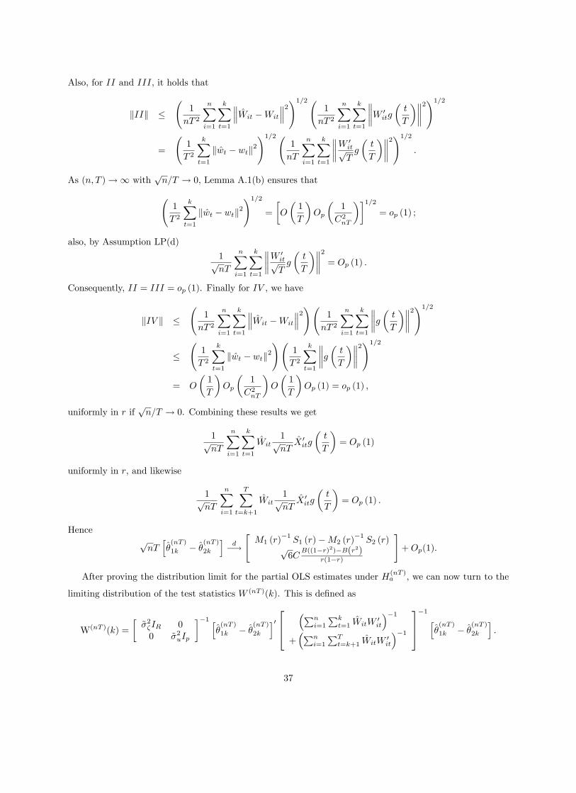
Also, for II and III, it holds that
kIIk �
1
nT 2
nXi=1
kXt=1
Wit �Wit
2!1=2 1
nT 2
nXi=1
kXt=1
W 0itg
�t
T
� 2!1=2
=
1
T 2
kXt=1
kwt � wtk2!1=2
1
nT
nXi=1
kXt=1
W 0itpTg
�t
T
� 2!1=2
:
As (n; T )!1 withpn=T ! 0, Lemma A.1(b) ensures that 1
T 2
kXt=1
kwt � wtk2!1=2
=
�O
�1
T
�Op
�1
C2nT
��1=2= op (1) ;
also, by Assumption LP(d)
1pnT
nXi=1
kXt=1
W 0itpTg
�t
T
� 2 = Op (1) :Consequently, II = III = op (1). Finally for IV , we have
kIV k �
1
nT 2
nXi=1
kXt=1
Wit �Wit
2! 1
nT 2
nXi=1
kXt=1
g� tT� 2
!1=2
� 1
T 2
kXt=1
kwt � wtk2!
1
T 2
kXt=1
g� tT� 2
!1=2
= O
�1
T
�Op
�1
C2nT
�O
�1
T
�Op (1) = op (1) ;
uniformly in r ifpn=T ! 0. Combining these results we get
1pnT
nXi=1
kXt=1
Wit1pnTX 0itg
�t
T
�= Op (1)
uniformly in r, and likewise
1pnT
nXi=1
TXt=k+1
Wit1pnTX 0itg
�t
T
�= Op (1) :
HencepnTh�(nT )
1k � �(nT )
2k
id�!"M1 (r)
�1S1 (r)�M2 (r)
�1S2 (r)p
6CB((1�r)2)�B(r2)
r(1�r)
#+Op(1):
After proving the distribution limit for the partial OLS estimates under H(nT )a , we can now turn to the
limiting distribution of the test statistics W (nT )(k). This is de�ned as
W(nT )(k) =
�~�2�IR 0
0 ~�2uIp
��1 h�(nT )
1k � �(nT )
2k
i0 264�Pn
i=1
Pkt=1 WitW
0it
��1+�Pn
i=1
PTt=k+1 WitW
0it
��1375�1 h
�(nT )
1k � �(nT )
2k
i:
37
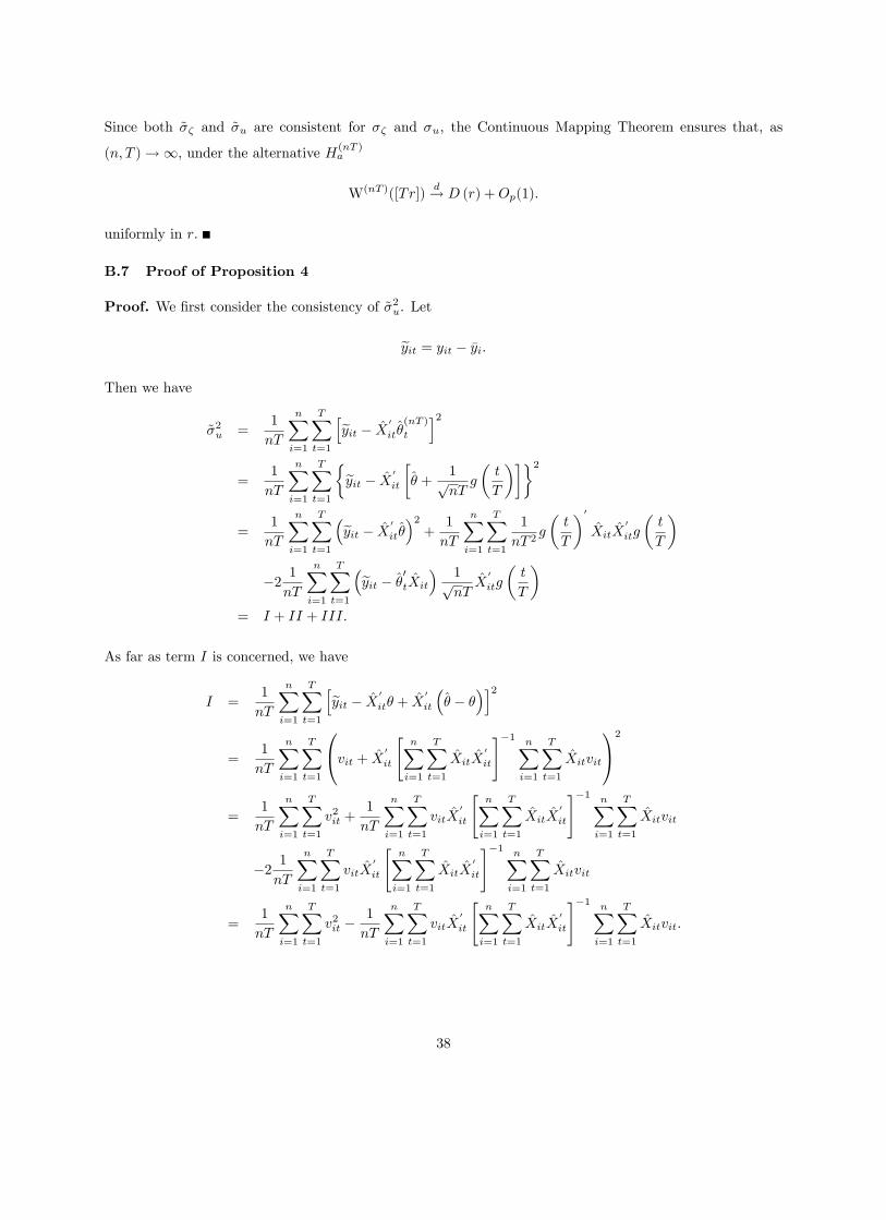
Since both ~�� and ~�u are consistent for �� and �u, the Continuous Mapping Theorem ensures that, as
(n; T )!1, under the alternative H(nT )a
W(nT )([Tr])d! D (r) +Op(1):
uniformly in r.
B.7 Proof of Proposition 4
Proof. We �rst consider the consistency of ~�2u. Let
eyit = yit � �yi:Then we have
~�2u =1
nT
nXi=1
TXt=1
heyit � X 0
it�(nT )
t
i2=
1
nT
nXi=1
TXt=1
�eyit � X 0
it
�� +
1pnTg
�t
T
���2
=1
nT
nXi=1
TXt=1
�eyit � X 0
it��2+
1
nT
nXi=1
TXt=1
1
nT 2g
�t
T
�0
XitX0
itg
�t
T
�
�2 1nT
nXi=1
TXt=1
�eyit � �0tXit� 1pnTX
0
itg
�t
T
�= I + II + III:
As far as term I is concerned, we have
I =1
nT
nXi=1
TXt=1
heyit � X 0
it� + X0
it
�� � �
�i2
=1
nT
nXi=1
TXt=1
0@vit + X 0
it
"nXi=1
TXt=1
XitX0
it
#�1 nXi=1
TXt=1
Xitvit
1A2
=1
nT
nXi=1
TXt=1
v2it +1
nT
nXi=1
TXt=1
vitX0
it
"nXi=1
TXt=1
XitX0
it
#�1 nXi=1
TXt=1
Xitvit
�2 1nT
nXi=1
TXt=1
vitX0
it
"nXi=1
TXt=1
XitX0
it
#�1 nXi=1
TXt=1
Xitvit
=1
nT
nXi=1
TXt=1
v2it �1
nT
nXi=1
TXt=1
vitX0
it
"nXi=1
TXt=1
XitX0
it
#�1 nXi=1
TXt=1
Xitvit:
38

As far as III is concerned, it holds that
1
nT
nXi=1
TXt=1
�eyit � X 0
it�� 1p
nTX
0
itg
�t
T
�
=1
nT
nXi=1
TXt=1
24vit + X 0
it
nXi=1
TXt=1
XitX0
it
!�1 nXi=1
TXt=1
Xitvit
35 1pnTX
0
itg
�t
T
�
=1
nT
nXi=1
TXt=1
1pnTg
�t
T
�0Xitvit
+1
nT
"nXi=1
TXt=1
1pnTg
�t
T
�0XitX
0
it
#"nXi=1
TXt=1
XitX0
it
#�1 " nXi=1
TXt=1
Xitvit
#:
Combing I with II and III we get
~�2u =1
nT
nXi=1
TXt=1
v2it
� 1
nT
nXi=1
TXt=1
vitX0
it
"nXi=1
TXt=1
XitX0
it
#�1 nXi=1
TXt=1
Xitvit
+1
nT
nXi=1
TXt=1
1
nT 2g
�t
T
�0
XitX0
itg
�t
T
�
� 2
nT
nXi=1
TXt=1
1pnTg
�t
T
�0Xitvit
� 2
nT
"nXi=1
TXt=1
1pnTg
�t
T
�0XitX
0
it
#"nXi=1
TXt=1
XitX0
it
#�1 " nXi=1
TXt=1
Xitvit
#:
Now
1
nT
nXi=1
TXt=1
vitX0
it
"nXi=1
TXt=1
XitX0
it
#�1 nXi=1
TXt=1
Xitvit = Op
�1
nT
�;
use Lemma A.4;
1
nT
nXi=1
TXt=1
1
nT 2g
�t
T
�0
XitX0
itg
�t
T
�= Op
�1
nT
�;
use Assumption LP(d);
1
nT
nXi=1
TXt=1
1pnTg
�t
T
�0Xitvit = Op
�1pnT
�;
use Assumption LP(e);
1
nT
"nXi=1
TXt=1
1pnTg
�t
T
�0XitX
0
it
#"nXi=1
TXt=1
XitX0
it
#�1 " nXi=1
TXt=1
Xitvit
#= Op
�1
nT
�;
due to Lemma A.4 and Assumption LP(b). Hence
~�2u =1
nT
nXi=1
TXt=1
v2it + op (1) ;
39

and it holds that
1
nT
nXi=1
TXt=1
v2it =1
nT
nXi=1
TXt=1
h�0�Xit � Xit
�+ uit
i2=
1
nT
nXi=1
TXt=1
�h�0(wt � wt)
i2+ u2it + 2�
0(wt � wt)uit
�2
=1
nT
nXi=1
TXt=1
u2it +1
T
TXt=1
h�0(wt � wt)
i2+
2
nT
nXi=1
TXt=1
�0(wt � wt)uit
= I + II + III:
For I, use Assumption M1 and a LLN we have
I = �2u + op (1) :
As far as II and III are concerned, we have
kIIk � k�k2 1T
TXt=1
k(wt � wt)k2 = op (1)
using Lemma A.1(b), and
kIIIk � k�k2 1
nT
TXt=1
k(wt � wt)k2!1=2 nX
i=1
TXt=1
u2it
!1=2= op (1) ;
after equation (25). Then under the local alternatives H(nT )a it holds that
~�2up�! �2u:
We are now ready also to prove consistency of ~�2� . Since
~�2� = ~�2u + �
(nT )0�2��
(nT );
and since
�2�p�! �2�
under H(nT )a as it does not depend on H(nT )
a being true or not, in light of the consistency of �(nT )
we have
~�2�p�! �2u + �
(nT )0�2��(nT )0 = �2� :
40

References
[1] Andrews, D. W. K. (1993), �Tests for Parameter Instability and Structural Changes with Unknown
Change Point,�Econometrica, 61, 821-856.
[2] Andrew, D. W. K. and Ploberger, W. (1994), �Optimal Tests When a Nuisance Parameter is Present
Only Under the Alternative,�Econometrica, 62, 1383-1414.
[3] Audrino, F., Barone-Adesi, G., and Mira, A. (2005), �The Stability of Factors of Interest Rates,�Journal
of Financial Econometrics, 3, 422-441.
[4] Bai, J. (2003), �Inferential Theory for Structural Models of Large Dimensions�, Econometrica, 71,
135-171.
[5] Bai, J. (2004), �Estimating Cross-Section Common Stochastic Trends in Nonstationary Panel Data,�
Journal of Econometrics, 122, 137-183.
[6] Bai, J. (2006), �Common Breaks in Panel Data,�Working paper.
[7] Bai, J., and Ng, S. (2002), �Determining the Number of Factors in Approximate Factor Models,�
Econometrica, 70, 191-221.
[8] Bai, J., and Ng, S. (2004), �A Panic Attack on Unit Roots and Cointegration�, Econometrica, 72,
1127-1178.
[9] Benerjee, A., and Urga, G. (2005), "Modelling Structural Breaks, Long Memory and Stock Market
Volatility: An Overview�, Journal of Econometrics, 129, 1-34.
[10] Chiang, M-H., McCoskey, S., Kao, C. (2002), �Panel Data Tests for a Common Break point in a
Cointegrated Regression: Asymptotic and Small Sample Results.�manuscript.
[11] Emerson, J., and Kao, C. (2001), �Testing for Structural Change of a Time Trend Regression in Panel
Data: Part I,�Journal of Propagations in Probability and Statistics, 2, 57�75.
[12] Emerson, J., and Kao, C. (2002), �Testing for Structural Change of a Time Trend Regression in Panel
Data: Part II,�Journal of Propagations in Probability and Statistics, 2, 207-250.
[13] Hall, P., and Heyde, C. C. (1980), Martingale Limit Theory and Its Applications, New York: Academic
Press.
[14] Han, A. K., and Park, D. (1989), �Testing for Structural Change in Panel Data: Application to a Study
of U.S. Foreign Trade in Manufacturing Goods,�Review of Economics and Statistics, 71, 135-142.
41

[15] Hansen, B. (1999), �Threshold E¤ects in Non-Dynamic Panels: Estimation, testing and Inference,�
Journal of Econometrics, 93, 345-368.
[16] Joseph, L. and Wolfson, D. B. (1992), �Estimation in Multi-Path Change-Point Problems,� Comm.
Statist. Theory Methods, 21, 897-913.
[17] Joseph, L. and Wolfson, D. B. (1993), �Maximum Likelihood Estimation in the Multi-Path Changepoint
Problem,�Ann. Inst. Statist. Math., 45, 511-530.
[18] Joseph, L., Wolfson, D. B., Berger, R. D., and Lyle, R. M. (1997), �Analysis of Panel Data with
Change-Points,�Statistica Sinica, 7, 687-703.
[19] Kao, C. (1999), �Spurious Regression and Residual-Based Tests for Cointegration in Panel Data�,
Journal of Econometrics, 90, 1-44.
[20] Kao, C., and Chiang, M. H. (2000), �On the Estimation and Inference of a Cointegrated Regression in
Panel Data,�Advances in Econometrics, 15, 179-222.
[21] Kao, C., Trapani, L. and Urga, G. (2006), " Asymptotics for Panel Models with Common Shocks",
WP-CEA-01-2006, Centre for Econometric Analysis, Cass Business School.
[22] Litterman, R., and Scheinkman, J. A. (1991), �Common Factors A¤ecting Bond Returns,�Journal of
Fixed Income, 1, 54-61.
[23] Moon, H. R., and Perron, B. (2004), �Testing for a Unit Root in Panels with Dynamic Factors,�Journal
of Econometrics, 122, 81-126.
[24] Phillips, P. C. B., and Moon, H. R. (1999), �Linear Regression Limit Theory for Nonstationary Panel
Data,�Econometrica, 67, 1057-1112.
[25] Perignon, C., and Villa, C. (2006), �Sources of Time Variation in the Covariance Matrix of Interest
Rates�, Journal of Business, 79, 1535-1549.
[26] Perron, P. (2006), "Dealing with Breaks", Chapter 8 in the Palgrave Handbook of Econometrics: Vol. 1
Econometric Theory edited by T.C. Mills and K. Patterson, Palgrave Macmillan: Basingstoke.
[27] Stock, J. H., and Watson, M. W. (1999), �Forecasting In�ation,�Journal of Monetary Economics, 44,
293-335.
[28] Stock, J. H., and Watson, M. W. (2002), �Forecasting Using Principal Components From a Large
Number of Predictors,�Journal of the American Statistical Association, 97, 1167-1179.
42

[29] Stock, J. H., and Watson, M. W. (2005), �Implications of Dynamic Factor Models for Var Analysis,�
Working paper.�
[30] Wachter, S. D., and Tzavalis, E. (2004), �Detection of Structural Breaks in Linear Dynamic Panel Data
Models,�Working Paper No. 505, Queen Mary, University of London.
43

TABLE 1:
Size at the 5% Level
Panel A: Size for SupWnnT 20 40 60 120 240 48020 0.0175 0.0375 0.0372 0.0637 0.0587 0.051940 0.0145 0.0236 0.0248 0.0462 0.0514 0.060460 0.0149 0.0260 0.0340 0.0337 0.0397 0.0550120 0.0151 0.0287 0.0346 0.0373 0.0470 0.0561240 0.0172 0.0309 0.0306 0.0360 0.0480 0.0454480 0.0212 0.0285 0.0351 0.0349 0.0501 0.0560
Panel B: Size for AveWnnT 20 40 60 120 240 48020 0.0267 0.0375 0.0350 0.0490 0.0407 0.035040 0.0258 0.0267 0.0242 0.0342 0.0349 0.040360 0.0220 0.0273 0.0312 0.0299 0.0265 0.0339120 0.0238 0.0298 0.0315 0.0325 0.0306 0.0354240 0.0241 0.0333 0.0330 0.0311 0.0367 0.0314480 0.0312 0.0300 0.0307 0.0298 0.0375 0.0349
Panel C: Size for ExpWnnT 20 40 60 120 240 48020 0.0306 0.0472 0.0455 0.0653 0.0537 0.045840 0.0272 0.0325 0.0534 0.0475 0.0461 0.052560 0.0241 0.0353 0.0392 0.0337 0.0352 0.0455120 0.0269 0.0388 0.0428 0.0396 0.0411 0.0473240 0.0289 0.0427 0.0403 0.0362 0.0453 0.0405480 0.0370 0.0403 0.0415 0.0377 0.0489 0.0460
44

TABLE 2:
Power at 5% Level
Panel A. Power for SupWnnT 20 40 60 120 240 48020 0.0715 0.2085 0.4723 0.7962 0.9972 1.000040 0.0850 0.2332 0.5129 0.9467 1.0000 1.000060 0.0932 0.3281 0.6545 0.9837 1.0000 1.0000120 0.1340 0.5551 0.8512 0.9999 1.0000 1.0000240 0.2545 0.9640 0.9697 1.0000 1.0000 1.0000480 0.4195 0.9327 0.9996 1.0000 1.0000 1.0000
Panel B. Power for AveWnnT 20 40 60 120 240 48020 0.0859 0.2170 0.4477 0.8364 0.9983 1.000040 0.1055 0.2699 0.5523 0.9655 1.0000 1.000060 0.1172 0.3693 0.6917 0.9927 1.0000 1.0000120 0.1686 0.6003 0.8921 1.0000 1.0000 1.0000240 0.2991 0.8142 0.9877 1.0000 1.0000 1.0000480 0.4700 0.9637 1.0000 1.0000 1.0000 1.0000
Panel C. Power for ExeWnnT 20 40 60 120 240 48020 0.1009 0.2448 0.4993 0.8321 0.9980 1.000040 0.1224 0.2838 0.5628 0.9620 1.0000 1.000060 0.1329 0.3874 0.7006 0.9910 1.0000 1.0000120 0.1806 0.6151 0.8899 1.0000 1.0000 1.0000240 0.3168 0.8131 0.9850 1.0000 1.0000 1.0000480 0.4894 0.9599 0.9999 1.0000 1.0000 1.0000
45