CENTRE FOR ECONOMETRIC ANALYSIS CEA@Cass

http://www.cass.city.ac.uk/cea/index.html

Cass Business School Faculty of Finance 106 Bunhill Row

London EC1Y 8TZ

Identification-Robust Factor Pricing: Canadian Evidence

Marie-Claude Beaulieu, Jean-Marie Dufour and Lynda Khalaf

CEA@Cass Working Paper Series

WP–CEA–02-2015

Identification-Robust Factor Pricing: CanadianEvidence∗

Marie-Claude Beaulieu †

Université LavalJean-Marie Dufour ‡

McGill University

Lynda Khalaf §

Carleton University

May 26, 2015

∗ This work was supported by the Institut de Finance Mathématique de Montréal [IFM2], theNatural Sciences and Engineering Research Council of Canada, the Social Sciences and Humani-ties Research Council of Canada, the Fond Banque Royale en Finance and the Fonds FQRSC andNATECH (Government of Québec). The authors thank Marie-Hélène Gagnon for providing Cana-dian data on the Fama-French and Momentum factors, and Mark Blanchette for excellent researchassistance.† Centre Interuniversitaire de Recherche sur les Politiques Économique et de l’Emploi (CIR-

PÉE), Département de finance et assurance, Pavillon Palasis-Prince, local 3632, Université Laval,Québec, Canada G1K 7P4. TEL: (418) 656-2131-2926, FAX: (418) 656-2624. email: Marie-Claude.Beaulieu@fas.ulaval.ca‡ Centre interuniversitaire de recherche en économie quantitative (CIREQ), Centre interuniver-

sitaire de recherche en analyse des organisations (CIRANO), William Dow Professor of Economics,Department of Economics, McGill University. Mailing address: Leacock Building, Rm 519, 855Sherbrooke Street West, Montréal, Québec, Canada H3A 2T7. TEL: (514) 398 8879; FAX: (514)398 4938; e-mail: jean-marie.dufour@mcgill.ca.§ Groupe de recherche en économie de l’énergie, de l’environnement et des ressources na-

turelles (GREEN) Université Laval, Centre interuniversitaire de recherche en économie quanti-tative (CIREQ), and Economics Department, Carleton University. Mailing address: EconomicsDepartment, Carleton University, Loeb Building 1125 Colonel By Drive, Ottawa, Ontario, K1S5B6 Canada. Tel (613) 520-2600-8697; FAX: (613)-520-3906. email: Lynda_Khalaf@carleton.ca.

ABSTRACT

We analyze Arbitrage Pricing Theory (APT) based factor models using identificationrobust inference methods. Such models involve nonlinear reduced rank restrictionswhose identification may raise serious non-regularities leading to the failure of stan-dard asymptotics. We next derive confidence set estimates for structural parametersbased on inverting, analytically, Hotelling-type type pivotal statistics. Proposedconfidence sets have much more informational content than Hotelling-type tests, andextend their relevance beyond reduced forms. Our approach may further be viewedas a multivariate extension of the Fieller problem. We also introduce a formal de-finition for a redundant factor linking the presence of such factors to unboundedestimation outcomes and document their perverse effects on minimum-root-basedmodel tests. Results are applied to multi-factor asset pricing models with Canadiandata, the Fama-French-Carhart benchmarks and monthly returns of 25 portfoliosfrom 1991 to 2010.Despite evidence of weak identification, several results deserve notice when data is

analyzed over 10 year sub-periods. With equally weighted portfolios, the three-factormodel is rejected before 2000 and weakly supported thereafter. In contrast, the threefactor model is not rejected with value weighted portfolios. Interestingly in this case,the market factor is priced before 2000 along with size, while both Fama-Frenchfactors are priced thereafter. The momentum factor severely compromises identifica-tion, which calls for caution in interpreting existing work documenting momentumeffects for the Canadian market. More generally, our empirical analysis underscorethe practical usefulness of our analytical confidence sets.

i

1 Introduction

Equilibrium based financial econometric models commonly involve reduced rank

(RR) restrictions. Well known applications include asset pricing works related to the

Arbitrage Pricing Theory (APT) and to factor models [Black (1972), Ross (1976)].1

From a methodological perspective, RR restrictions raise serious statistical chal-

lenges. Even with linear multivariate models, discrepancies between standard asymp-

totic and finite sample distributions can be very severe and are usually attributed

to the curse of dimensionality; see e.g. Dufour & Khalaf (2002) and the references

therein. Nonlinear rank restrictions pose further identification non-regularities that

can lead to the failure of standard asymptotics. This provides the motivation for our

paper.

From an empirical perspective, we focus on RR-based inference methods relevant

to asset pricing factor models. In general multivariate regression based financial

models, finite sample motivated testing is important because tests that are only

approximate and/or do not account for non-normality can lead to unreliable empirical

interpretations of standard financial models; see e.g. Shanken (1996), Campbell

et al. (1997), Dufour et al. (2003), Dufour et al. (2010) and Beaulieu et al. (2007),

Beaulieu et al. (2009), Beaulieu et al. (2010a), Beaulieu et al. (2013). In parallel, an

emerging literature that builds on Kan & Zhang (1999a) and Kan & Zhang (1999b)

recognizes the adverse effects of a large number of factors; see Kleibergen (2009),

Kan et al. (2013), Gospodinov et al. (2014), Kleibergen & Zhan (2013) and Harvey

et al. (2015). We consider inference methods immune to both dimensionality and

identification diffi culties.1See also Gibbons (1982), Barone-Adesi (1985), Shanken (1986), Zhou (1991), Zhou (1995),

Bekker et al. (1996), Costa et al. (1997), (Campbell et al. 1997, Chapter 6), Velu & Zhou (1999),and Shanken & Zhou (2007).

1

The few finite sample rank-based asset pricing methods [see e.g. Zhou (1991),

Zhou (1995), Shanken (1985), Shanken (1986) and Shanken & Zhou (2007)] have for

the most part focused on testing rather than on set inference. Kleibergen (2009)

provides numerical identification-robust inference methods backed by a simulation

study that reinforces the motivation for our asset-pricing focus.2 Beaulieu et al.

(2013) proposes a confidence set estimate approach, yet the weakly identified para-

meter is scalar because of a single-factor restriction. In the present paper our results

cover parameter vectors, which expands the class of applicable financial models.

Overall, the paper has three main contributions.

First, we construct confidence set (CS) estimates for the model’s parameters

of interest, based on inverting minimum-distance pivotal statistics. These include

Hotelling’s T2 criterion [Hotelling (1947)]. In multivariate analysis, Hotelling’s sta-

tistic is mostly used for test purposes, and its popularity stems from its least-squares

(LS) foundations which lead to exact F-based null distributions in Gaussian set-

tings. We apply analytical solutions to the test inversion problem. Our CSs provides

much more information than Hotelling-type tests, and extend their relevance beyond

reduced form specifications; see Beaulieu et al. (2015) for underlying finite sample

theory and simulation evidence.

Second, we provide a formal definition of a statistically non-informative factor

and linking the presence of such factors to unbounded set estimation outcomes. We

also document the perverse effects of adding such factors on J-type minimum-root-

based model tests. Although unbounded set estimators are not always uninformative,

our results call for caution in relying on model tests alone as measures of fit. This

warning has obvious implications for the asset pricing models that motivate our

empirical analysis, which we further illustrate empirically.

Third, our results are applied to multi-factor asset pricing models with Canadian

data and the benchmark Fama-French-Carhart [Fama & French (1992), Fama &

2In contrast, Kan et al. (2013), Gospodinov et al. (2014) and Kleibergen & Zhan (2013) focuson model misspecification.

2

French (1993), Carhart (1997)] model. We analyze monthly returns of 25 portfolios

from 1991 to 2010. The empirical literature on asset pricing models in Canada is

scarce. Most studies involving Canadian assets aim to measure North-American fi-

nancial market integration (see for example Jorion & Schwartz (1986), Mittoo (1992)

and Foerster & Karolyi (1993) and more recently Beaulieu et al. (2008)). In some

other cases, for example, Griffi n (2002) and Fama & French (2012) international mul-

tifactor asset pricing models are tested over a large set of countries including Canada

to measure the importance of international versus domestic asset pricing factors in

different countries.

One of the few articles that relate the importance of a multifactor asset pricing

model for Canadian portfolios using exclusively Canadian factors is L’Her et al.

(2004); for a larger set of papers, see the references therein. We propose to enlarge

this strand of literature to verify on a long time period the importance of domestic

Fama and French factors to price Canadian assets adding momentum to the list of

factors included in L’Her et al. (2004). The specificities of Canadian assets are put

forward and contrasted to American assets for which abundant results are available

in the literature. To achieve this goal we use, as described above, improved inference

procedures based on a formal definition of a statistically non-informative asset pricing

factor.

With reference to the weak-instruments literature, our methodology may be

viewed as a generalization of the Dufour & Taamouti (2005) quadrics-based set

estimation method beyond the linear limited information simultaneous equations

setting. For further quadric based solutions in different contexts, see Bolduc et al.

(2010) for inference on multiple ratios, and Khalaf & Urga (2014) for inference on

cointegration vectors.

With reference to Kleibergen (2009), our methodology allows to estimate the

zero-beta rate [Shanken (1992), (Campbell et al. 1997, Chapter 6) or Lewellen et al.

(2010)], which has not been considered by Kleibergen (2009). Theoretically coherent

3

empirical models often impose restrictions on the risk-prices via the zero-beta rate;

see e.g. (Lewellen et al. 2010, prescription 2). Examples include: (i) whether the

zero beta rate is equal to the risk-free rate, and (ii) whether the risk price of a traded

portfolio when included as a factor equals the factor’s average return in excess of the

zero-beta rate [Shanken (1992)]. We also formally control for factors that are trad-

able portfolios. Furthermore, in contrast to Kleibergen’s numerical projections, our

analytical solutions can easily ascertain empty or unbounded sets, whereas numeri-

cal solutions remain subject to precision and execution time constraints. Avoiding

numerical searches is particularly useful for multi-factor models.

With reference to the statistical literature, our test inversion approach can be

viewed as an extension of the classical inference procedure proposed by Fieller (1954)

[see also Zerbe et al. (1982), Dufour (1997), Beaulieu et al. (2013), Bolduc et al.

(2010)] to the multivariate setting. As with standard χ2-type methods including e.g.

the delta method, our generalized Fieller approach relies on LS. Yet both methods

exploit LS theory in fundamentally different ways. In contrast to the former which ex-

cludes parameter discontinuity regions out and which by construction yields bounded

confidence intervals, our inverted test does not require parameter identification and

allows for unbounded solutions.

Empirically, despite overwhelming evidence of weak identification, several inter-

esting results deserve notice particularly when data is analyzed over 10 year sub-

periods. With equally weighted portfolios, the three-factor model is rejected before

2000. Thereafter, the model is weakly supported with HML confirmed as the only

priced factor. With value weighted data, the three factor model is not rejected;

interestingly, the market factor is priced before 2000 and unidentified thereafter,

while both Fama-French factors are priced post 2000. Although momentum is priced

with equally-weighted data before 2000, the resulting sets on other factors are practi-

cally uninformative. The momentum factor thus severely compromises identification,

which calls for caution in interpreting existing work documenting momentum effects

4

for the Canadian market.

The paper is organized as follows. Section 2 sets the notation and framework.

In section 3 we present our test inversion method and associated projections. Our

empirical analysis is discussed in section 4. Section 5 concludes followed by a technical

appendix.

2 Multifactor pricing model

Let ri, i = 1, . . . , n, be a vector of T returns on n assets or portfolios for t =

1, . . . , T , and R =[R1 ... Rq

]a T × q matrix of observations on q risk factors.

Building on multivariate regressions of the form

ri = aiιT +Rbi + ui, i = 1, . . . , n, (1)

our APT based empirical analysis formally accounts for tradable factors; see Shanken

(1992), (Campbell et al. 1997, Chapter 6) and Lewellen et al. (2010) and note that

the inference method applied by Kleibergen (2009) relaxes tradability restrictions.

Without loss of generality, suppose that R1 corresponds to a vector of returns ona tradable portfolio, for example, a market benchmark. Partition R into R1 and Fso the latter T × (q − 1) submatrix contains the observations on the (q − 1) factors[R2 ... Rq

]and partition bi conformably into the scalar bi1 and the (q − 1)

dimensional vector biF . In this context, the APT implies a zero-intercept in the

regression of returns in excess of the zero-beta rate, denoted γ0, on: (i) R1 in excessof γ0, and (ii) onR2, ...,Rq in excess of a risk price (q−1) dimensional vector denoted

γF , where γ0 and γF are unknown parameters:

ri − ιTγ0 = (R1 − ιTγ0) bi1 + (F − ιTγ′F) biF + ui, i = 1, . . . , n. (2)

Rewriting the latter in the (1) form produces a non-linear RR restriction on its

5

intercept that captures the zero-beta rate and risk premia as model parameters:

ri = aiιT +R1bi1 + FbiF + ui, (3)

ai + γ0(bi1 − 1) + γ′FbiF = 0. (4)

Here we derive confidece set estimators for the q-dimensional vector

θ = (γ0, γ′F)′ (5)

which we interpret via a traditional cross-sectional factor pricing approach [see e.g.

(Campbell et al. 1997, Chapter 6) or Shanken & Zhou (2007)]. Indeed, the time

series averages of (3) leads (with obvious notation) to

ri = γ0(1− bi1)− γ′FbiF + R1bi1 + FbiF + ui, i = 1, . . . , n (6)

= γ0 +(R1 − γ0

)bi1 +

(F−γ′F

)biF + ui, i = 1, . . . , n.

It follows that γ0 retains its traditional cross-sectional definition, and the coeffi cients

on betas of the non-tradable factors correspond to(F − γ′F

). This implies that R1

is not priced if R1 − γ0 = 0 and each of the remaining factors will be not be priced

in turn, if the corresponding components of F −γ′F = 0. Our procedure as described

below yields confidence intervals on γ0 and on the components of γF . Given these

intervals, we assess whether the tradable factor is not priced if R1 is covered, andwhether each factor besides R1 is not priced if the average of each factor is, in turn,not covered.

Our intervals are simultaneous in the sense of joint coverage, which implies that

decisions on pricing will also be simultaneous. A formal definition of simultaneity

is further discussed in the next section which outlines our confidence set estimation

method.

3 Identification, estimation and testing

Whether viewed as a RR multivariate or cross sectional regression, identification of

θ can be assessed within (2) or (6). If bi1 ' 1 then γ0 almost drops out of the model.

6

Furthermore, if any of the factor betas is close to zero across i, its risk price effectively

drops out. In fact, whenever factor betas bunch up across or within test assets,

problems akin to cross-sectional colinearity emerge that undermine identification of

θ. As may be checked within (6), for θ to be recoverable with no further data and

information (in particular in the absence of other instruments), the betas per factor

need to vary enough across equation. In practice, reliance on portfolios to reduce

dimensionality ends up reducing dispersion of betas. Identification concerns are thus

an empirical reality.

To address this problem, we extend Beaulieu et al. (2013) beyond the single factor

and scalar parameter case. In particular, we proceed by inverting a multivariate test

of a hypothesis that fixes θ to a given value, say θ0:

H0 (θ0) : θ = θ0, θ0 known. (7)

Inverting the test in question at a given level α consists in assembling the θ0 values

that are not rejected at this level. For example, given a right-tailed statistic T (θ0)

with α-level critical point Tc, our procedure involves solving, over θ0, the inequality

T (θ0) < Tc (8)

where Tc controls size for any θ0. The solution results in a parameter space subset,denoted CS (θ;α), that satisfies

P[θ ∈ CS ( θ;α)

]≥ 1− α (9)

whether θ is identified or not.

To derive confidence intervals for the individual components of θ, or more gen-

erally, for a given scalar function g (θ), we proceed by projecting CS ( θ;α), that is,

by minimizing and maximizing g (θ) over the θ values in CS ( θ;α). The resulting

intervals so obtained are simultaneous, in the following sense: for any set of m con-

tinuous real valued functions of θ, gi (θ) ∈ R, i = 1, ...,m, let gi(

CS (θ;α))denote

7

the image of CS (θ;α) by the function gi. Then

P[gi (θ) ∈ gi

(CS (θ;α)

), i = 1, . . . , m

]≥ 1− α. (10)

If Tc is defined so that (9) holds without identifying θ then (10) would also holdwhether θ is identified or not. A complete description of our methodology requires:

(i) defining T (θ0), (ii) deriving Tc to control size for any θ0, and (iii) characterizingthe solution of (8). As in Beaulieu et al. (2013), we find an analytical solution to all

of the above.

We focus on the Hotelling-type statistic

Λ (θ) =(1, θ′)BS−1B′(1, θ′)′

(1, θ′)(X ′X)−1(1, θ′)′(11)

where θ is set by (7)

B = (X ′X)−1X ′Y , S = U ′U , U = Y −XB, (12)

X is a T × k full-column rank matrix that includes a constant regressor and the

observations on all q factors so k = q+ 1, and Y is the T × n matrix that stacks theleft-hand side returns in deviation from the tradable benchmark. Clearly, B and U

are the OLS estimators for the underlying unrestricted reduced form

Y = XB + U ⇔ Yt = B′Xt + Ut, t = 1, . . . , T (13)

where U is the disturbance matrix and the restriction on the intercept (3) is rewritten

as (1, θ′)B = 0 in which case (7) corresponds to

H0 (θ0) : (1, θ′0)B = 0, θ0 known.

We rely on the F -approximation

Λ (θ)τnn∼ F (n, τn) , τn = T − k − n+ 1. (14)

8

which holds exactly when the regression errors Ut are contemporaneously correlated

i.i.d. Gaussian assuming we can condition on X for statistical analysis. The lat-

ter distributional result does not require any identification restriction.3 For proofs

and further references, see Beaulieu et al. (2015) and references therein. Simula-

tion studies reported in this paper confirm that fat tailed disturbances arising from

multivariate-t or GARCH do not cause size distortions for empirically relevant de-

signs.

Λ (θ) can be interpreted relative to the financial literature and in particular the

well known zero-intercept test of Gibbons et al. (1989), as follows. The classical

Hotelling statistics which provide multivariate extensions of the Student-t based

significance tests take the form

Λ0j =sk[i]

′BS−1B′sk[i]

sk[i]′(X ′X)−1sk[i]. (15)

where sk[j] denotes a k-dimensional selection vector with all elements equal to zero

except for the j-th element which equals 1. The underlying hypotheses assess the

joint contribution of each factor in (13), that is

H0j : sk[j]′B = 0, j ∈ {1, ..., k} . (16)

So for example sk[1] provides inference on the unrestricted intercept, and sk[2] allows

one to assess the betas on the tradable factor in deviation from one; see Beaulieu

et al. (2010a) for recent applications. The same null distribution as in (14) also

holds for each of the Λ0j (under the above same conditions). Interestingly, we show

that inverting Λ (θ) embeds all of these tests via a suffi cient condition for bounded

outcomes that avoids pre-testing.

To invert (11)-(14) we rewrite the inequation

Λ (θ) ≤ fn,τn,α (17)

3Other than the usual Least Squares assumptions on X ′X and S.

9

where fn,τn,α denotes the α-level cut off point from the F (n, τn) distribution as

(1, θ′)A(1, θ′)′ ≤ 0 (18)

where A is the k × k data dependent matrix

A = BS−1B′ − (X ′X)−1fn,τn,α (n/τn) . (19)

Simple algebraic manipulations suffi ce to show the above. Next, inequality (18) is

re-expressed as

θ′A22θ + 2A12θ + A11 ≤ 0 (20)

which leads to the set-up of Dufour & Taamouti (2005) so projections based CSs

for any linear transformation of θ can be obtained as described in this papers. The

solution is reproduced in the Appendix for completion. This requires partitioning A

as follows

A =

[A11 A12A21 A22

](21)

where A11 is a scalar, A22 is q × q, and A12 = A′21 is 1× q. Using the partitioning

B =

[a′

b

], b =

β′2...β′k

(22)

where a′ is 1× q and conformably

(X ′X)−1 =

[x11 x12

x21 x22

](23)

where x11 is a scalar, x21 = x12′ is q × 1 and x22 is q × q, we have A11 = a′S−1a −(fn,τn,α (n/τn))x11, A12 = A′21 = a′S−1b′ − (fn,τn,α (n/τn))x12 and

A22 = bS−1b′ − (fn,τn,α (n/τn))x22. (24)

The outcome of resulting projections can be empty, bounded, or the union of

two unbounded disjoint sets. Dufour & Taamouti (2005) show that outcomes are

10

unbounded if A22 is not positive definite. Applying basic algebra again to (24)

reveals that the diagonal terms of A22 are

Fj = sk[j]′BS−1B′sk[j]− sk[j]′(X ′X)−1sk[j]

nfn,τn,ατn

, j = 1, ..., k.

Comparing this expression to the definition of Λ0j in (15) implies that

Λ0j (τn) /n < fn,τn,α ⇔ Fj < 0, j = 1, ..., k.

So if any of the classical Hotelling tests, using the distribution in (14), is not signif-

icant at level α, then A22 cannot be positive definite and the confidence set will be

unbounded. That is, if the tradable beta is not significantly different from one over

all portfolios or if any of the factors is jointly redundant, then information on the

zero beta rate as well as the risk price for all factors is compromised. The above

condition is suffi cient but not necessary. It follows that although Hotelling tests on

each factor are useful, the information they provide is incomplete as for the joint

usefulness of the factors in identifying risk price.

An important result from Beaulieu et al. (2013) regarding empty confidence set

outcomes also generalizes to our multifactor case. Because the cut-off point under-

lying the inversion of Λ (θ) , which we denoted fn,τn,α above, is the same for all θ

values, then

minθ

Λ (θ) ≥ fn,τn,α ⇔ CS (θ;α) = ∅.

Again, basic matrix algebra allows one to show [see e.g. Gouriéroux et al. (1996)] that

minimizing Λ (θ) produces the Gaussian-LR statistic to test the non-linear restriction

(3) which defines θ. This suggests a bounds J-type test to assess the overall model

fit. The outcome of this test will be revealed via the quadric solution we implement

for test inversion, so it is built into our general set inference procedure. A potential

unbounded confidence set guards the researcher from misreading nonsignificant tests

as evidence in favour of models on which data is not informative.

11

In summary, our confidence sets will summarize the data’s informational content

(from a least-squares or Gaussian quasi-likelihood perspective) on risk price without

compounding type-I errors.

4 Empirical analysis

In our empirical analysis of a multifactor asset pricing model, we use Canadian

Fama and French (1992, 1993) factors as well as momentum (Carhart, 1997). We

produce results for monthly returns of 25 value weighted portfolios from 1991 to

2010. Portfolios were constructed with all Canadian stocks available on Datastream

and Worldscope. The portfolios which are constructed at the end of June are the

intersections of five portfolios formed on size (market equity) and five portfolios

formed on the ratio of book equity to market equity. The size breakpoints for year

s are the Toronto Stock Exchange (TSE) market equity quintiles at the end of June

of year s. The ratio of book equity to market equity for June of year s is the book

equity for the last fiscal year end in s− 1 divided by market equity for December of

year s−1. The ratios of book equity to market equity are TSE quintiles. We use the

filter from Karolyi & Wu (2014) to eliminate abnormal observations in our database.

This filter is minimally invasive as the filtered database contains an overall sample

average of 1700 stocks.

The benchmark factors are: 1) the excess return on the market, defined as the

value-weighted return on all TSE stocks (from Datastream andWorldscope database)

minus the one-month Treasury bill rate (from the Bank of Canada), 2) SMB (small

minus big) defined as the average return on three small portfolios minus the average

return on three big portfolios, 3) HML (high minus low) defined as the average return

on two value portfolios minus the average return on two growth portfolios, and (4),

MOM, the average return on the two high prior return portfolios minus the average

return on the two low prior return portfolios. Fama and French benchmark factors,

SMB and HML, are constructed from six size/book-to-market benchmark portfolios

12

that do not include hold ranges and do not incur transaction costs. The portfolios for

these factors are rebalanced annually using two independent sorts, on size (market

equity, ME) and book-to-market (the ratio of book equity to market equity, BE/ME).

The size breakpoint (which determines the buy range for the small and big portfolios)

is the median TSE market equity. The BE/ME breakpoints (which determine the

buy range for the growth, neutral, and value portfolios) are the 30th and 70th TSE

percentiles. For the construction of the MOM factor, six value-weighted portfolios

formed on size and prior (2—12) returns are used. The portfolios, which are formed

monthly, are the intersections of two portfolios formed on size (market equity, ME)

and three portfolios formed on prior (2—12) return. The monthly size breakpoint is

the median TSE market equity. The monthly prior (2—12) return breakpoints are

the 30th and 70th TSE percentiles.

Results over 10 and 5 years subperiods are summarized in Tables 1 and 2, where

EW and VW denotes equally weighted and value weighted portofolios. Unless stated

otherwise, signficance in what what follows refers to the 5% level. All reported

confidence sets are also at the 5% level.

Over 10 year subperiods and with equally-weighted data, the three-factor model

is rejected before 2000. Thereafter, while very wide although bounded confidence

intervals are observed, HML is confirmed as the only priced factor. Value weighted

data supports the three factor model before 2000 albeit weakly as all confidence sets

obtained are unbounded. Interestingly, the market factor is priced along with SMB.

In sharp contrast, the market risk is unidentified after 2000 and despite evidence of

identification diffi culties, both Fama-French factors are priced. When the momentum

factor is added over and above the Fama-French factor, we find completely uninfor-

mative results on all model parameters expect for momentum using equally-weighted

data before 2000, in which case we find this factor is priced despite the overwhelming

evidence of weak-identification.

Considering 5 year subperiods may help us assess whether the above is driven by

13

instability of betas. Results must however be interpreted with caution since sample

size considerations can be consequential. Indeed, the bulk of resulting confidence sets

are uninformative and the only evidence we can confirm is that the market factor

seems to be priced from 1996-2000 while the HML factor is priced post 2006.

Our empirical results collected together reveal that to price Canadian assets, a

standard three Fama and French factor model is the best avenue after 2000. Mo-

mentum creates important identification problems and it should not be used to price

Canadian assets without raising identification questions. This corroborates the em-

pirical results of Beaulieu et al. (2010b) and Beaulieu et al. (2015) for American

stocks although the case for omitting momentum is stronger in the Canadian con-

text. An important issue further analyzed by Beaulieu et al. (2015) for the U.S. is

the portfolio formation method. Using industry portfolios seems to improve identifi-

cation relative to size-sorting, as the latter compounds factor structure dependences;

see also Lewellen & Nagel (2006), Lewellen et al. (2010) and Kleibergen & Zhan

(2013).

On balance, given the importance of Fama and French factors for pricing stocks

internationally [Fama & French (2012)], and the potential for identification problems

presented in this paper, future research should aim at finding ways of choosing the

factors that empirically explain the cross-section of returns in a general standard

context, as discussed in Harvey et al. (2015).

5 Conclusion

This paper studies the factor asset pricing model for the Canadian market using

identification robust inference methods. We derive confidence sets for the zero beta

rate and factor price based on inverting minimum-distance Hotelling-type pivotal

statistics. We use analytical solutions to the latter problem. Our confidence sets

have much more informational content than usual Hotelling tests and have various

useful applications in statistics, econometrics and finance. Our approach further

14

provides multivariate extensions of the classical Fieller problem.

Empirical results illustrate, among others, severe problems with redundant fac-

tors. These finding concur with the (above cited) emerging literature on redundant

factors, on tight factor structures and statistical pitfalls of asset pricing tests, and

on the importance of joint (across-portfolios) tests. In practice, our results support

a standard three Fama and French factor model for the Canadian market after 2000.

In contrast, we find that the momentum factor severely compromises identification

which qualifies existing works in this regard.

With regards to the historical debate on the market factor4, our results suggest

an alternative perspective. Perhaps the unconditional market model is neither dead

nor alive and well. Instead, the traditional methods of accounting for additional

factors may have confounded underlying inference. Because traditional methods

severely understate true uncertainty, identification problems in the literature may

have escaped concrete notice so far. More to the point here is that with reference to

e.g. Harvey et al. (2015) who consider a very large number of factors, we document

identification problems with only three to four factors. We thus concur with (Lewellen

et al. 2010, prescriptions 5 and 6) that it is by far more useful to report set estimates

rather than model tests. However, the proliferation of factors in practice increases the

likelihood of redundancies. Their associated costs support the use of our method,

and motivate further refinements and improvements as important future research

avenues.

4See (Campbell et al. 1997, Chapters 5 and 6), Fama & French (2004), Perold (2004), Campbell(2003) and Sentana (2009).

15

Table 1. Confidence sets for risk premia

Ten years sub-periods

ri − ιTγ0 = (R1 − ιTγ0) bi1 + (F − ιTγ′F) biF + ui, i = 1, . . . , n

θ = (γ0, γ′F)′ = (θMKT, θSMB, θHML)′

EW MKT SMB HML MOM×10−4 R1 θMKT F θSMB F θHML F -91-00 51 ∅ 25 ∅ 28 ∅ -56 -00-10 48 [-1165, 302] 149 [-105, 786] 218* [-1750, 187] -9 -VW MKT SMB HML MOM×10−4 R1 θMKT F θSMB F θHML F -91-00 51* ]−∞,−521] 25* ]−∞, 15] 28 ]−∞, 419] -56 -

∪ [13490,∞[ ∪ [4284,∞[ ∪ [7601,∞[00-10 48 R 149* ]−∞,-711] 218* ]−∞, -1611] -9 -

∪ [526,∞[ ∪ [3056,∞[

θ = (γ0, γ′F)′ = (θMKT, θSMB, θHML, θHML)′

EW MKT SMB HML MOM×10−4 R1 δ F δ F δ F δ91-00 51 R 25 R 28 R -56* ]−∞, -969]

∪ [415,∞[00-10 48 R 149 R 218 R -9 RVW MKT SMB HML MOM×10−4 R1 δ F δ F δ F δ91-00 51 R 25 R 28 R -56 R00-10 48 R 149 R 218 R -9 R

Note: Sample includes monthly observations from January 1991 to December 2010.

Series are constructed with all Canadian observations from Datastream and Worldscope.

They include 25 equally weighted (EW) and value weighted (VW) portfolios as well as

Canadian factors for market (MKT), size (SMB), book-to-market (HML) and momentum

(MOM). Confidence sets are at the 5% level. F is the factor average over the considered

time period; θcaptures factor pricing as defined in (5). * denotes evidence of pricing at the

5% significance level interpreted as follows: given the reported confidence sets, the tradable

factor is not priced if R1is covered; each other factor is not priced if (its average) is not

covered; see section 2.

16

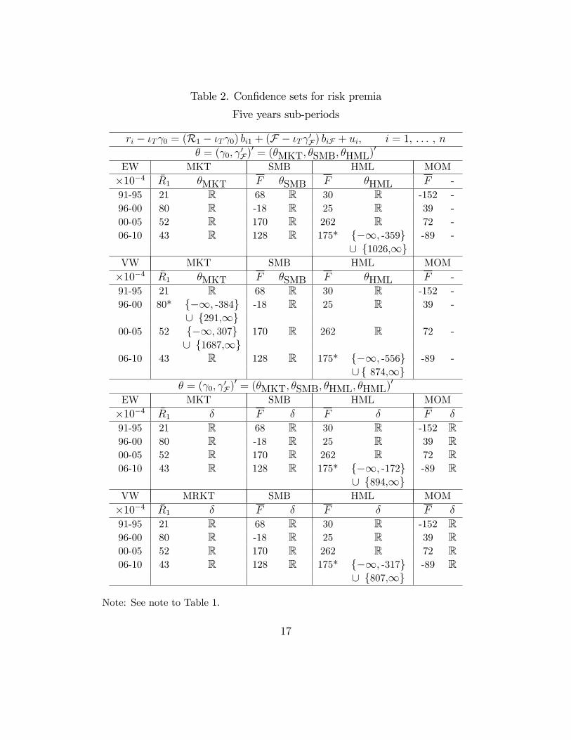
Table 2. Confidence sets for risk premia

Five years sub-periods

ri − ιTγ0 = (R1 − ιTγ0) bi1 + (F − ιTγ′F) biF + ui, i = 1, . . . , n

θ = (γ0, γ′F)′ = (θMKT, θSMB, θHML)′

EW MKT SMB HML MOM×10−4 R1 θMKT F θSMB F θHML F -91-95 21 R 68 R 30 R -152 -96-00 80 R -18 R 25 R 39 -00-05 52 R 170 R 262 R 72 -06-10 43 R 128 R 175* {−∞, -359} -89 -

∪ {1026,∞}VW MKT SMB HML MOM×10−4 R1 θMKT F θSMB F θHML F -91-95 21 R 68 R 30 R -152 -96-00 80* {−∞, -384} -18 R 25 R 39 -

∪ {291,∞}00-05 52 {−∞, 307} 170 R 262 R 72 -

∪ {1687,∞}06-10 43 R 128 R 175* {−∞, -556} -89 -

∪{ 874,∞}θ = (γ0, γ

′F)′ = (θMKT, θSMB, θHML, θHML)′

EW MKT SMB HML MOM×10−4 R1 δ F δ F δ F δ91-95 21 R 68 R 30 R -152 R96-00 80 R -18 R 25 R 39 R00-05 52 R 170 R 262 R 72 R06-10 43 R 128 R 175* {−∞, -172} -89 R

∪ {894,∞}VW MRKT SMB HML MOM×10−4 R1 δ F δ F δ F δ91-95 21 R 68 R 30 R -152 R96-00 80 R -18 R 25 R 39 R00-05 52 R 170 R 262 R 72 R06-10 43 R 128 R 175* {−∞, -317} -89 R

∪ {807,∞}

Note: See note to Table 1.

17

18

Appendix

This appendix summarizes the solution of (20) from Dufour & Taamouti (2005).

Projections based confidence sets for any linear transformation of θ of the form ω′θ

can be obtained as follows. Let A = −A−122 A′12, D = A12A−122 A12 − A11. If all the

eigenvalues of A22 [as defined in (21)] are positive so A22 is positive definite then:

CSα(ω′θ) =

[ω′A−

√D(ω′A−122 ω

), ω′A+

√D(ω′A−122 ω

)], if D ≥ 0 (A1)

CSα(ω′θ) = ∅, if D < 0. (A2)

If A22 is non-singular and has one negative eigenvalue then: (i) if ω′A−122 ω < 0 and

D < 0:

CSα(ω′θ) =

]−∞, ω′A−

√D(ω′A−122 ω

)]∪[ω′A+

√D(ω′A−122 ω

),+∞

[; (A3)

(ii) if ω′A−122 ω > 0 or if ω′A−122 ω ≤ 0 and D ≥ 0 then:

CSα(ω′θ) = R; (A4)

(iii) if ω′A−122 ω = 0 and D < 0 then:

CSα(ω′θ) = R\{ω′A

}. (A5)

The projection is given by (A4) if A22 is non-singular and has at least two negative

eigenvalues.

19

References

Barone-Adesi, G. (1985), ‘Arbitrage equilibrium with skewed asset returns’, Journal

of Financial and Quantitative Analysis 20(3), 299—313.

Beaulieu, M.-C., Dufour, J.-M. & Khalaf, L. (2007), ‘Multivariate tests of mean-

variance effi ciency with possibly non-Gaussian errors: An exact simulation-based

approach’, Journal of Business and Economic Statistics 25, 398—410.

Beaulieu, M.-C., Dufour, J.-M. & Khalaf, L. (2009), ‘Finite sample multivariate

tests of asset pricing models with coskewness’, Computational Statistics and Data

Analysis 53, 2008—2021.

Beaulieu, M.-C., Dufour, J.-M. & Khalaf, L. (2010a), ‘Asset-pricing anomalies and

spanning: Multivariate multifactor tests with heavy tailed distributions’, Journal

of Empirical Finance 17, 763—782.

Beaulieu, M.-C., Dufour, J.-M. & Khalaf, L. (2010b), Identification-robust estima-

tion and testing of the Zero-Beta CAPM, Technical report, Mc Gill University,

Université Laval and Carleton University.

Beaulieu, M.-C., Dufour, J.-M. & Khalaf, L. (2013), ‘Identification-robust estimation

and testing of the Zero-Beta CAPM’, The Review of Economics Studies 80, 892—

924.

Beaulieu, M.-C., Dufour, J.-M. & Khalaf, L. (2015), Weak beta, strong beta: factor

proliferation and rank restrictions, Technical report, Mc Gill University, Université

Laval and Carleton University.

Beaulieu, M.-C., Gagnon, M.-H. & Khalaf, L. (2008), ‘A cross-section analysis of

financial market integration in north america using a four factor model’, Interna-

tional Journal of Managerial Finance 5, 248—267.

20

Bekker, P., Dobbelstein, P. &Wansbeek, T. (1996), ‘The APTmodel as reduced-rank

regression’, Journal of Business and Economic Statistics 14, 199—202.

Black, F. (1972), ‘Capital market equilibrium with restricted borrowing’, Journal of

Business 45, 444—454.

Bolduc, D., Khalaf, L. & Yelou, C. (2010), ‘Identification robust confidence sets meth-

ods for inference on parameter ratios with application to discrete choice models’,

Journal of Econometrics 157, 317—327.

Campbell, J. Y. (2003), ‘Asset pricing at the millennium’, Journal of Finance

55, 1515—1567.

Campbell, J. Y., Lo, A. W. & MacKinlay, A. C. (1997), The Econometrics of Finan-

cial Markets, Princeton University Press, New Jersey.

Carhart, M. M. (1997), ‘On persistence in mutual fund performance’, Journal of

Finance 52, 57—82.

Costa, M., Gardini, A. & Paruolo, P. (1997), ‘A reduced rank regression approach to

tests of asset pricing’, Oxford Bulletin of Economics and Statistics 59, 163—181.

Dufour, J.-M. (1997), ‘Some impossibility theorems in econometrics, with applica-

tions to structural and dynamic models’, Econometrica 65, 1365—1389.

Dufour, J.-M. & Khalaf, L. (2002), ‘Simulation based finite and large sample tests

in multivariate regressions’, Journal of Econometrics 111, 303—322.

Dufour, J.-M., Khalaf, L. & Beaulieu, M.-C. (2003), ‘Exact skewness-kurtosis tests

for multivariate normality and goodness-of-fit in multivariate regressions with ap-

plication to asset pricing models’, Oxford Bulletin of Economics and Statistics

65, 891—906.

21

Dufour, J.-M., Khalaf, L. & Beaulieu, M.-C. (2010), ‘Multivariate residual-based

finite-sample tests for serial dependence and GARCH with applications to asset

pricing models’, Journal of Applied Econometrics 25, 263—285.

Dufour, J.-M. & Taamouti, M. (2005), ‘Projection-based statistical inference in linear

structural models with possibly weak instruments’, Econometrica 73, 1351—1365.

Fama, E. F. & French, K. R. (1992), ‘The cross-section of expected stock returns’,

Journal of Finance 47, 427—465.

Fama, E. F. & French, K. R. (1993), ‘Common risk factors in the returns on stocks

and bonds’, Journal of Financial Economics 33, 3—56.

Fama, E. F. & French, K. R. (2004), ‘The capital asset pricing model: Theory and

evidence’, Journal of Economic Perspectives 18, 25—46.

Fama, E. F. & French, K. R. (2012), ‘Size, value and momentum in international

stock returns’, Journal of Financial Economics 105, 457—472.

Fieller, E. C. (1954), ‘Some problems in interval estimation’, Journal of the Royal

Statistical Society, Series B 16(2), 175—185.

Foerster, S. & Karolyi, A. (1993), ‘International listings of stocks: the case of canada

and the u.s.’, Journal of International Business Studies 24, 763—784.

Gibbons, M. R. (1982), ‘Multivariate tests of financial models: A new approach’,

Journal of Financial Economics 10, 3—27.

Gibbons, M. R., Ross, S. A. & Shanken, J. (1989), ‘A test of the effi ciency of a given

portfolio’, Econometrica 57, 1121—1152.

Gospodinov, N., Kan, R. & Robotti, C. (2014), ‘Misspecification-robust inference

in linear asset-pricing models with irrelevant risk factors’, Review of Financial

Studies 27, 2139—2170.

22

Gouriéroux, C., Monfort, A. & Renault, E. (1996), Tests sur le noyau, l’image et le

rang de la matrice des coeffi cients d’un modèle linéaire multivarié, Oxford Univer-

sity press, Oxford (U.K.).

Griffi n, J. (2002), ‘Are the fama and french factors global or country specific?’, Review

of Financial Studies 15, 783—803.

Harvey, C. R., Liu, Y. & Zhu, H. (2015), ‘...and the cross-section of expected returns.

review of financial studies’, Review of Financial Studies Forthcoming.

Hotelling, H. (1947), Multivariate Quality Control Illustrated by the Air Testing of

Sample Bomb Sights,Techniques of Statistical Analysis, Ch. II, McGraw-Hill, New

York.

Jorion, P. & Schwartz, E. (1986), ‘Integration versus segmentation in the canadian

stock market’, Journal of Finance 41, 603—640.

Kan, R., Robotti, C. & Shanken, J. (2013), ‘Pricing model performance and

the two-pass cross-sectional regression methodology’, The Journal of Finance

68, 2617âAS2649.

Kan, R. & Zhang, C. (1999a), ‘GMM tests of stochastic discount factor models with

useless factors’, Journal of Financial Economics 54(1), 103—127.

Kan, R. & Zhang, C. (1999b), ‘Two-pass tests of asset pricing models with useless

factors’, Journal of Finance 54, 204—235.

Karolyi, A. & Wu, Y. (2014), Size, value, and momentum in international stock

returns: A partial segmentation approach, Technical report, Cornell University.

Khalaf, L. & Urga, G. (2014), ‘Identification robust inference in cointegrating regres-

sions’, Journal of Econometrics 182, 385—396.

23

Kleibergen, F. (2009), ‘Tests of risk premia in linear factor models’, Journal of Econo-

metrics 149, 149—173.

Kleibergen, F. & Zhan, Z. (2013), Unexplained factors and their effects on second

pass r-squared’s and t-tests, Technical report, Brown University.

Lewellen, J., Nagel, S. & Shanken, J. (2010), ‘A skeptical appraisal of asset-pricing

tests’, Journal of Financial Economics 92, 175—194.

Lewellen, J. W. & Nagel, S. (2006), ‘The conditional CAPM does not explain asset-

pricing anomalies’, Journal of Financial Economics 82, 289—314.

L’Her, J. F., Masmoudi, T. & Suret, J.-M. (2004), ‘Evidence to support the four-

factor pricing model from the canadian market’, Journal of International Financial

Markets, Institutions and Money 14, 313—328.

Mittoo, U. (1992), ‘Additional evidence in the canadian stock market.’, Journal of

Finance 47, 2035—2054.

Perold, A. F. (2004), ‘The capital asset pricing model’, Journal of Economic Per-

spectives 18, 3—24.

Ross, S. A. (1976), ‘The arbitrage theory of capital asset pricing’, Journal of Eco-

nomic Theory 13, 341—360.

Sentana, E. (2009), ‘The econometrics of mean-variance effi ciency tests: A survey’,

Econometrics Journal 12, C65—C101.

Shanken, J. (1985), ‘Multivariate tests of the zero-beta CAPM’, Journal of Financial

Economics 14, 325—348.

Shanken, J. (1986), ‘Testing portfolio effi ciency when the zero-beta rate is unknown:

A note’, Journal of Finance 41, 269—276.

24

Shanken, J. (1992), ‘On the estimation of beta-pricing models’, Review of Financial

Studies 5, 1—33.

Shanken, J. (1996), Statistical methods in tests of portfolio effi ciency: A synthesis, in

G. S. Maddala & C. R. Rao, eds, ‘Handbook of Statistics 14: Statistical Methods

in Finance’, North-Holland, Amsterdam, pp. 693—711.

Shanken, J. & Zhou, G. (2007), ‘Estimating and testing beta pricing models: Al-

ternative methods and their performance in simulations’, Journal of Financial

Economics 84, 40—86.

Velu, R. & Zhou, G. (1999), ‘Testing multi-beta asset pricing models’, Journal of

Empirical Finance 6, 219—241.

Zerbe, G. O., Laska, E., Meisner, M. & Kushner, H. B. (1982), ‘On multivariate

confidence regions and simultaneous confidence limits for ratios’, Communications

in Statistics, Theory and Methods 11, 2401—2425.

Zhou, G. (1991), ‘Small sample tests of portfolio effi ciency’, Journal of Financial

Economics 30, 165—191.

Zhou, G. (1995), ‘Small sample rank tests with applications to asset pricing’, Journal

of Empirical Finance 2, 71—93.

25