ISSN 1440-771X

Australia

Department of Econometrics and Business Statistics

http://www.buseco.monash.edu.au/depts/ebs/pubs/wpapers/

February 2014

Working Paper 06/14

A Class of Demand Systems Satisfying Global Regularity And Having Complete Rank Flexibility

Keith R. McLaren and Ou Yang

Corresponding author: Keith R. McLaren, Department of Econometrics and Business Statistics, Monash University, Clayton campus, Wellington Road, Clayton, Victoria 3800, Australia. Tel +61 3 99052395. E-mail Address: Keith.McLaren@monash.edu

A Class of Demand Systems Satisfying Global Regularity

and Having Complete Rank Flexibility

Keith R. McLaren* and Ou Yang

Department of Econometrics and Business Statistics, Monash University, Australia

December 24 2013

Abstract: A class of demand systems based on simple parametric specification of the indirect

utility functions, but allowing for the parsimonious imposition of global regularity, is

proposed. Demand systems in this class are completely flexible in rank, i.e., can be

potentially specified to acquire as large a rank as required in empirical work. They also

exhibit a clear and reasonable homothetic asymptotic behaviour. In an empirical application

using Australian data, several examples from this class are estimated and compared with

some popular alternatives in the literature.

Keywords: Demand systems; Global regularity; Complete rank flexibility; Duality theory;

Indirect utility function

JEL classification: D11, D12

1

I. Introduction

Microeconomic theory sets up a solid foundation for the estimation of systems of

demand equations. This theory, in its most transparent form, states that such demand

equations should be consistent with the maximization of utility subject to a budget

constraint. Accordingly, a demand system is deemed to be regular if it satisfies the

restrictions imposed by the paradigm of rational consumer choice. In the context of

Marshallian demand systems, this means the demand systems expressing quantities

demanded as functions of expenditure and prices satisfy the properties of non-negativity,

homogeneity, Engel aggregation, Cournot aggregation, and the symmetry and negative

semi-definiteness of the Slutsky matrix (Deaton and Muellbauer 1980).

To translate these restrictions into empirical application, three approaches may be

identified. In the first approach, the demand equations are derived literally by specifying a

direct utility function and solving the constrained maximization problem. Although this

approach leads to demand systems which satisfy the above regularity conditions by

construction, the need to derive analytical solutions to the first order conditions restricts its

application to quite specific utility functions. To our knowledge, the derivation and

estimation of consumer demand systems from globally regular direct utility functions which

satisfy everywhere the neoclassical monotonicity and curvature conditions are restricted to

minor variants of Cobb-Douglas and C.E.S forms, and they come at the price of inflexibility.

For instance, in a Leontief system the ratios of quantities of commodities are always in fixed

proportions, irrespective of price or income; in a Cobb-Douglas system income, own-price

and cross-price elasticities are a priori constrained to be unity, minus one and zero,

respectively.

The second approach is the Rotterdam methodology, which attempts to impose the

regularity restrictions on log-differential approximations to the demand equations. This

approach, first proposed by Theil (1965) and Barten (1966), has frequently been used to test

the theory. This approach, in many ways, is very similar to Stone’s (1954) method, but it

works in differentials, instead of working in levels of logarithms. The main query that can be

raised with respect to the Rotterdam methodology is: given the numerous

parameterizations used in applications, does the particular parameterization chosen

correspond to a legitimate parameterization of preferences, i.e. of the direct or indirect

utility functions; in other words, are the functional forms used integrable? Answering this

query is not a trivial task, and to our knowledge, it hasn’t been properly answered in the

literature, yet.

The third approach exploits the theory of duality among direct utility functions, indirect

utility functions, and cost functions, and the regularity conditions on these functions which

make them equivalent representations of the underlying preferences. Duality theory allows

systems of demand equations to be derived from these dual representations via simple

2

differentiation, according to Roy’s Identity or Shephard’s Lemma. This approach was

popularized by Diewert (1974, 1982), and led to the use of flexible functional forms, such as

the Generalized Leontief of Diewert (1971) and the Translog of Christensen, Jorgenson, and

Lau (1975), in that they do not impose any prior restrictions on slopes or elasticities at a

point of approximation, and hence they can potentially be regular at this point. In other

words, they possess enough free parameters to attain arbitrary elasticities at a point in

price-expenditure space, by providing a second-order approximation to an arbitrary twice

continuously differentiable cost or indirect utility function (Diewert and Wales 1987).

However, this flexibility at a point comes at the cost that such systems generally satisfy

globally only homogeneity with respect to prices and expenditures, and often violate

monotonicity and, particularly, curvature restrictions, either within the sample, or at points

close to the sample. Lau (1986) discusses the characterization of regularity of such systems,

and shows that the domain of regularity is rather limited.

In an attempt to resolve this conflict, much work has attempted to improve regularity,

in the context of curvature, for example, the Fourier expansions used by Gallant (1981,

1984), Elbadawi, Gallant, & Souza (1983) and Gallant & Golub (1984), Barnett’s minflex

Laurent expansion (Barnett, 1983; Barnett, 1985; Barnett & Lee, 1985), the Generalized

McFadden and Generalized Barnett cost functions of Diewert and Wales (1987) and the

Asymptotically Ideal Model of Barnett and Yue (1988). However, Barnett (2002) shows that

without satisfaction of both curvature and monotonicity, the second-order conditions for

optimizing behaviour fail, and duality theory fails.

A convenient compromise is the class of “effectively globally regular” demand systems

(Cooper and McLaren 1992; Cooper and McLaren 1996; Cooper and McLaren 2006; McLaren

and Wong 2009). By “effectively globally regular” is meant that there exists a unit cost

function (or price index) ( )P p such that the regularity properties are satisfied for all

expenditure-price combinations satisfying ( )c P p , where c indicates expenditure and p

represents the vector of prices. Therefore, the regularity region is an unbounded region in

price-expenditure space, potentially including all points in the sample, and all points

corresponding to higher levels of “real income”. A well-known example of such a system is

the Linear Expenditure system (LES), which is regular over an unbounded region but only for

sufficiently high expenditure levels.

This paper, in the spirit of the third approach, introduces a class of demand systems

based on simple parametric specifications of the indirect utility functions, but allowing for

the parsimonious imposition of global regularity. This class of demand systems follow the

steps of AIDS due to Deaton and Muellbauer (1980), QUAIDS due to Banks, Blundell, and

Lewbel (1997), MAIDS due to Cooper and McLaren (1992) and Cooper and McLaren (1996),

and a more recent rank four demand system due to Lewbel (2003). Members from this class

can be specified to acquire as large a rank as required for empirical work, following the

3

definition of rank, due to Lewbel (1991) which generalizes Gorman’s rank to all demand

systems. They also exhibit a clear and valid homothetic asymptotic behaviour. Furthermore,

by using unit cost functions such as those suggested by Diewert and Wales (1987), this

approach can also allow complete price flexibility.

The layout of the paper is as follows. The parametric representation of the generic

indirect utility function in terms of unit cost functions is introduced in Section II, where

conditions for global regularity are specified. Section III details possible specifications for the

unit cost functions, and presents four specific examples, two of which are rank-two and the

rest are rank-three. For the purpose of illustration, in Section IV, using data from the

latest 2009-2010 Australian Household Expenditure Survey, the two rank-two and two

rank-three examples presented in Section III are estimated and compared with their existing

counterparts in the literature, namely LES, AIDS and QUAIDS.

II. The Representation of Preferences

Let m represent the number of goods, mp represent the corresponding vector of

prices, and let 0c represent total expenditure (cost), where m

is the positive orthant.

Based on duality theory, the approach to specifying demand systems based on dual

representation of preferences is typified by AIDS, a rank-two demand system. In particular,

the indirect utility function associated with the AIDS can be specified as:

1 2( , ) [ln( / ( ))] / ( )V c p c P p P p (1)

Where p is an m-vector of commodity prices, c is total expenditure, and 1P and 2P are

respectively specified as Translog and homogeneous of degree zero (HD0) Cobb-Douglas

functions of prices. AIDS is a special case of the PIGLOG specification, in which 1P and 2P are

explicitly specified, and PIGLOG is itself a special case of the PIGL (price independent

generalized linear) specification of Muellbauer (1975).

In spite of its dominance in empirical application, probably due to the very convenient

form of its share equations, especially for the linearized AIDS model, AIDS is not globally

regular. One may think that the violation of regularity by AIDS arises from the Translog

component, since it is well known that a Translog function cannot be globally regular, and

that the imposition of local (sample) regularity is a non-trivial task (Diewert and Wales 1987).

However, Even if 1P were specified along more regular lines following Diewert and Wales

(1987), the functional form (1) would still exhibit regularity violations. Briefly, the problem is

that 2P cannot be simultaneously HD0, non-decreasing, and concave in p. Euler’s theorem

rules out the HD0 and non-decreasing combination, and the HD0 and concave combination,

for any non-trivial functions. The full details can be found in Cooper and McLaren (1992).

4

Another popular model is QUAIDS, which is rank-three, and extends the AIDS share

equations to include a quadratic term of logarithmic real expenditure. The QUAIDS indirect

utility function can be specified as:

1 113

2

ln( / ( ))( , ) {[ ] ( )}

( )

c P pV c p P p

P p

(2)

where 1P and 2P are specified the same as in AIDS, and 3P is specified as another HD0 Cobb-

Douglas function. QUAIDS nests AIDS as a special case when 3 0P . Although attempting to

build consistency with observed Engel curves requiring quadratic terms in the logarithm of

expenditure, QUAIDS doesn’t help to gain any better regularity properties than AIDS.

Actually, by adding another HD0 Cobb-Douglas function of prices, it makes checking of

regularity conditions even more difficult. The more recent rank-four demand system, due to

Lewbel (2003), further extends QUAIDS along the same line by including a third HD1 Cobb-

Douglas, and is not regular either. Its indirect utility function can be specified as:

1 14 13

2

ln[( ( )) / ( )]( , ) {[ ] ( )}

( )

c P p P pV c p P p

P p

(3)

where 1P , 2P and 3P are specified as in QUAIDS, and 4 ( )P p is specified as a HD1 Cobb-Douglas.

By contrast, the class of “effectively globally regular” demand systems improves

regularity by proposing an indirect utility function which is comprised of expenditure and

unit cost functions, yet possesses an unbounded regularity region in price-expenditure

space, potentially including all points in the sample, and all points corresponding to higher

levels of “real income”, provided all the component unit cost functions satisfy several

sufficient regularity conditions. As an example of this class, the indirect utility function of

the Generalized Exponential Form due to Cooper and McLaren (1996) can be specified as:

1

2

( ) 1( )

( , ) ( )( )

c

P p cV c p

P p

(4)

where 1P and 2P are two unit cost functions satisfying several sufficient regularity conditions,

and 0 1, 1, and 0. The corresponding Marshallian demand equations are

regular over an unbounded region 1{( , ) : ( )}c p c P p . It is noteworthy that this effective

globally regular demand system is rank-two.

Following this line in the literature, we propose a class of demand systems, of which

the associated indirect utility functions are simple and parametric, and for which a simple

set of sufficient conditions will ensure global regularity, i.e., fully consistent with the

maximization of utility subject to a budget constraint over the entire price-expenditure

5

region. In addition, members of this class of demand systems are fully flexible in rank, i.e.,

can acquire as large a rank as required for empirical work.

The generic indirect utility function of this class is specified as follows:

10

( )( , ) ( ) ( )

( )k

nR k

k

k

P pcV c p

P p c

(5)

where parameters , 's and 's satisfy 0 and 0 1,k 0,k 1,..., .k n

According to duality theory, an indirect utility function ( , )V c p is a valid representation

of preferences if it satisfies the following regularity conditions: (i) continuous in ( , )c p , and

twice continuously differentiable everywhere except possibly at a set of specific price-

expenditure vectors of measure zero; (ii) HD0 in ( , )c p ; (iii) non-increasing in p ; (iv) non-

decreasing in c ; (v) quasi-convex in p . If ( , )V c p satisfies these regularity conditions over

the entire positive orthant 1 {( , ) : 0, 0}m c p c p

, ( , )V c p is said to be globally regular.

If ( , )V c p satisfies these regularity conditions over a region 1mR

, then ( , )V c p is said to

be locally regular. Flexible functional forms such as the Translog and Generalized Leontief

typically have rather restricted locally regular regions, and in particular those regular regions

are often bounded from above in the direction of real income.

For the specification in (5), sufficient conditions for global regularity will depend on the

properties of the ( )kP p functions, {0,..., }k n . These ( )kP p functions can be interpreted

as unit cost functions or price indices. The properties that a function ( )P p should satisfy to

qualify as a unit cost function (a price index) are: (i) ( )P p is continuous in p, and twice

continuously differentiable almost everywhere; (ii) ( ) 0P p for mp ; (iii) ( )P p is HD1;

(iv) ( )P p is non-decreasing in p; (v) ( )P p is concave in p; (vi) (1) 1P . In Appendix 1, it is

shown that provided that its component ( )kP p functions, {0,..., }k n , qualify as unit cost

functions, this generic indirect utility function ( , )RV c p in (5) satisfies all the regularity

conditions of an indirect utility function implied by the maximization of a utility function

subject to a budget constraint, over the entire price-expenditure space, and hence the

corresponding Marshallian demand equations are globally regular.

It is straightforward to see that the rank of this specification is 1n . As n is an arbitrary

integer, this model is fully flexible in rank. One may notice that this model seems to

resemble a series expansion approach, such as Barnett’s AIM. However, the ability of this

system specification to support arbitrary price functions, thus arbitrary rank, distinguishes it

from that of a series expansion approach. Moreover, as expenditure c goes to infinity, the

first part of the indirect utility function 0( / ( ))c P p dominates, and thus the rank of the

corresponding demand system degenerates to one. In other words, as income goes to

6

infinity, the preferences become homothetic, which can be regarded as a fairly reasonable

assumption about asymptotic (in c ) consumption behaviour.

Demand equations are most easily represented in share form. Application of Roy’s

Identity to (5) gives the associated share equations as:

0 0

0 0

( , ) ( ) ( , ) ( ) ( )

( , ) , 1,...,

( , ) ( ) ( , ) ( )

n n

k ki k k kiR k k

i i n n

k k k k

k k

R c p DP p R c p P p EP p

W c p p i m

R c p P p R c p P p

(6)

where 1

0 0( , ) ( )R c p c P p ; 1( , ) ( )k k

k k k kR c p c P p

, 1,...,k n ; /ki k iDP P p ,

0,...,k n ; ip is the price of good i , and ( ) ln ( ) / lnki k iEP p P p p , 0,...,k n (the

elasticity of price index k with respect to price of good i ).

From (6), it can be seen that in cases where Engel rank is less than or equal to two, the

share equations resemble the general share functional form of Lewbel’s fractional demand

systems in Lewbel (1987). Lewbel noted that fractional demands provide a parsimonious

way of increasing the range of Engel curve responses, and conjectured that they have

enhanced global regularity properties. System (6) demonstrates how such global regularity

properties can be imposed by restricting the component functions of prices to satisfy

properties other than just homogeneity.

It is noteworthy that (6) expresses a share, which is supposed to be naturally bounded

to the unit interval, as a weighted average of 1n functions of prices ( )kiEP p , which are

themselves bounded to the unit interval (the elasticities of non-decreasing, homogeneous

of degree one, price indices), with weights that are also bounded to the unit interval

provided 0 and 0 1,k 0,k 1,...,k n . Therefore, over the entire price-

expenditure space, the right-hand side of (6) is guaranteed to be within the unit interval.

This is a particularly serious issue for applied work, since policy evaluations are often

implemented towards the end of the sample or post-sample, at higher levels of real

expenditure.

By contrast, the share equations of AIDS, i.e. 1 2 1ln( / )i i iW EP EP c P , and those of

QUAIDS, i.e. 2

1 2 1 3 3 2 1ln( / ) ( / ) [ln( / )]i i i iW EP EP c P EP P P c P , will necessarily violate the

unit interval, as real expenditure grows, which, from one aspect, demonstrates their

inability to be globally regular (Banks, Blundell, and Lewbel 1997). Some other examples of

fractional demand systems (for example, Barnett and Jonas 1983 and Cooper and McLaren

1996) have share equations satisfying the zero-to-one range, whereas none with rank higher

than two have been specified and implemented empirically.

7

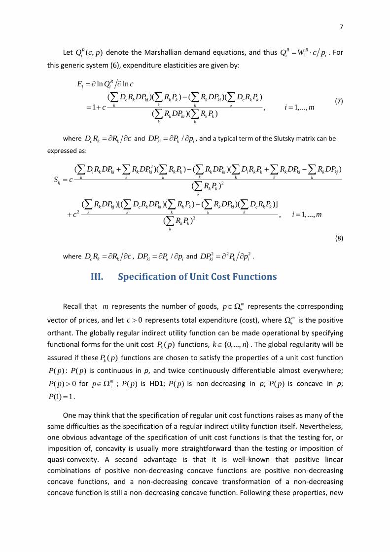
Let ( , )R

iQ c p denote the Marshallian demand equations, and thus R R

i i iQ W c p . For

this generic system (6), expenditure elasticities are given by:

ln ln

( )( ) ( )( )

1 , 1,...,( )( )

R

i i

c k ki k k k ki c k k

k k k k

k ki k k

k k

E Q c

D R DP R P R DP D R P

c i mR DP R P

(7)

where c k kD R R c and /ki k iDP P p , and a typical term of the Slutsky matrix can be

expressed as:

2

2

2

3

( )( ) ( )( )

( )

( )[( )( ) ( )( )]

, 1,...,( )

i k ki k ki k k k ki i k k k ki k kj

k k k k k k kij

k k

k

k kj c k ki k k k ki c k k

k k k k k

k k

k

D R DP R DP R P R DP D R P R DP R DP

S cR P

R DP D R DP R P R DP D R P

c i mR P

(8)

where c k kD R R c , /ki k iDP P p and 2 2 2

ki k iDP P p .

III. Specification of Unit Cost Functions

Recall that m represents the number of goods, mp represents the corresponding

vector of prices, and let 0c represents total expenditure (cost), where m

is the positive

orthant. The globally regular indirect utility function can be made operational by specifying

functional forms for the unit cost ( )kP p functions, {0,..., }k n . The global regularity will be

assured if these ( )kP p functions are chosen to satisfy the properties of a unit cost function

( )P p : ( )P p is continuous in p, and twice continuously differentiable almost everywhere;

( ) 0P p for mp ; ( )P p is HD1; ( )P p is non-decreasing in p; ( )P p is concave in p;

(1) 1P .

One may think that the specification of regular unit cost functions raises as many of the

same difficulties as the specification of a regular indirect utility function itself. Nevertheless,

one obvious advantage of the specification of unit cost functions is that the testing for, or

imposition of, concavity is usually more straightforward than the testing or imposition of

quasi-convexity. A second advantage is that it is well-known that positive linear

combinations of positive non-decreasing concave functions are positive non-decreasing

concave functions, and a non-decreasing concave transformation of a non-decreasing

concave function is still a non-decreasing concave function. Following these properties, new

8

valid and possibly complex unit cost functions can be constructed from known simple ones,

substantially extending the latitude of choice. In contrast, quasi-convexity is not preserved

when taking linear combinations.

In general, the choice of unit cost functions involves the usual trade-off between

regularity and flexibility. To allow complete price flexibility, one unit cost function could be

specified as Translog or more regular alternatives, such as the Generalized McFadden and

the Generalized Barnett, introduced by Diewert and Wales (1987). Even though some

regularity is sacrificed in this price flexible specification of our model, it is still inherently

more regular than its existing price flexible counterparts, such as AIDS or QUAIDS. From the

comparison in the next section, using the 2009-2010 Australian Household Expenditure

Survey data, it will be seen that the price flexible specification of this model outperforms its

existing price flexible counterparts in the literature.

For a rank-two specification of this model, a set of obvious and parsimonious initial

representations of the unit cost functions are the linear and Cobb-Douglas specifications

which are also used in LES. The details of this choice are presented below as Model 1. To

allow for complete price flexibility, one of the unit cost functions can be specified using one

of the flexible functions suggested by Diewert and Wales (1987), which can also be

constrained to satisfy curvature conditions globally.

Accordingly, Model 2 below is based on using the Generalized McFadden as the

specification for one of the two unit cost functions in a rank-two example of our model.

Since 0 ( )P p describes asymptotic behaviour, while 1( )P p can be interpreted as local

behaviour of a particular sample, it seems natural to consider the specification of 1( )P p

using a flexible functional form. In Model 3, a rank-three example, 0 ( )P p is specified as

Cobb-Douglas, and 1( )P p and 2 ( )P p are specified as CES which nests Cobb-Douglas and

linear specifications as special cases, while in Model 4, in order to allow comparability with

QUAIDS, 1( )P p and 2 ( )P p are respectively specified as Cobb-Douglas and Generalized

McFadden.

Model 1: Cobb-Douglas 0 ( )P p and linear 1( )P p :

0

11

( ) , 1, 0, 1,...,i

m m

i i i

ii

P p p i m

(9)

1

1 1

( ) , 1, 0, 1,...,m m

i i i i

i i

P p p i m

(10)

Hence, the specific indirect utility function is:

111 1 1

0

( )( , ) ( ) ( ) , , 0 1, 0.

( )

R P pcV c p

P p c

0 (11)

9

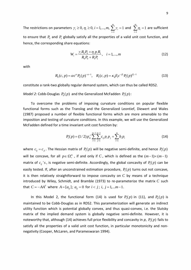
The restrictions on parameters 0,i 0, 1,..., ,i i m 1

1m

i

i

and 1

1m

i

i

are sufficient

to ensure that 0P and 1P globally satisfy all the properties of a valid unit cost function, and

hence, the corresponding share equations:

0 0 1

0 0 1 1

, 1,...,i i ii

R P p RW i m

R P R P

(12)

with

1 1 11

0 0 1 1 1 1( , ) ( ) , ( , ) ( )R c p c P p R c p c P p (13)

constitute a rank-two globally regular demand system, which can thus be called RDS2.

Model 2: Cobb-Douglas 0 ( )P p and the Generalized McFadden 1( )P p :

To overcome the problems of imposing curvature conditions on popular flexible

functional forms such as the Translog and the Generalized Leontief, Diewert and Wales

(1987) proposed a number of flexible functional forms which are more amenable to the

imposition and testing of curvature conditions. In this example, we will use the Generalized

McFadden defined for a time invariant unit cost function by:

1 1

1

1

1 1 1

( ) (1/ 2)m m m

m ij i j i i

i j i

P p p c p p b p

(14)

where ij jic c . The Hessian matrix of 1( )P p will be negative semi-definite, and hence 1( )P p

will be concave, for all mp , if and only if C , which is defined as the ( 1) ( 1)m m

matrix of 'ijc s , is negative semi-definite. Accordingly, the global concavity of 1( )P p can be

easily tested. If, after an unconstrained estimation procedure, 1( )P p turns out not concave,

it is then relatively straightforward to impose concavity on C by means of a technique

introduced by Wiley, Schmidt, and Bramble (1973) to re-parameterize the matrix C such

that TC AA where [ ]ijA a ; 0ija for i j ; , 1,... 1i j m .

In this Model 2, the functional form (14) is used for 1( )P p in (11), and 0 ( )P p is

maintained to be Cobb-Douglas as in RDS2. This parameterization will generate an indirect

utility function which is potential globally convex, and thus quasi-convex, i.e. the Slutsky

matrix of the implied demand system is globally negative semi-definite. However, it is

noteworthy that, although (14) achieves full price flexibility and concavity in p, 1( )P p fails to

satisfy all the properties of a valid unit cost function, in particular monotonicity and non-

negativity (Cooper, McLaren, and Parameswaran 1994).

10

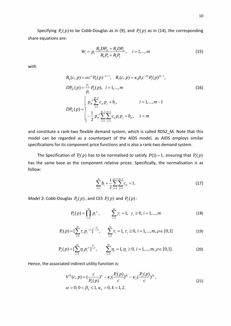
Specifying 0 ( )P p to be Cobb-Douglas as in (9), and 1( )P p as in (14), the corresponding

share equations are:

0 0 1 1

0 0 1 1

, 1,...,i ii i

R DP R DPW p i m

R P R P

(15)

with

1 1 11

0 0 1 1 1 1

0 0

11

1

1 1 11

1 1

( , ) ( ) , ( , ) ( ) ,

( ) ( ), 1,...,

, 1,..., 1

( )1

,2

ii

i

m

m ji j i

j

i m m

m ij i j m

i j

R c p c P p R c p c P p

DP p P p i mp

p c p b i m

DP p

p c p p b i m

(16)

and constitute a rank-two flexible demand system, which is called RDS2_M. Note that this

model can be regarded as a counterpart of the AIDS model, as AIDS employs similar

specifications for its component price functions and is also a rank-two demand system.

The Specification of 1( )P p has to be normalised to satisfy (1) 1P , ensuring that 1( )P p

has the same base as the component relative prices. Specifically, the normalisation is as

follow:

1 1

1 1 1

11.

2

m m m

i ij

i i j

b c

(17)

Model 3: Cobb-Douglas 0 ( )P p , and CES 1( )P p and 2 ( )P p :

0

11

( ) , 1, 0, 1,...,i

m m

i i i

ii

P p p i m

(18)

1

1

1 1

( ) [ ] , 1, 0, 1,..., , [0,1]m m

i i i i

i i

P p p i m

(19)

1

2

1 1

( ) [ ] , 1, 0, 1,..., , [0,1]m m

i i i i

i i

P p p i m

(20)

Hence, the associated indirect utility function is:

1 21 2

1 2

0

( ) ( )( , ) ( ) ( ) ( ) ,

( )

0; 0 1, 0, 1,2.

R

k k

P p P pcV c p

P p c c

k

(21)

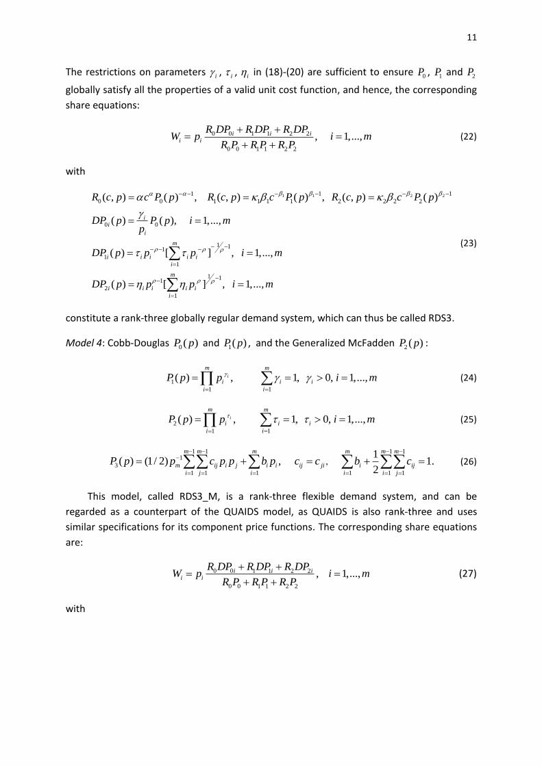
11

The restrictions on parameters i , i ,

i in (18)-(20) are sufficient to ensure 0P ,

1P and 2P

globally satisfy all the properties of a valid unit cost function, and hence, the corresponding

share equations:

0 0 1 1 2 2

0 0 1 1 2 2

, 1,...,i i ii i

R DP R DP R DPW p i m

R P R P R P

(22)

with

1 1 2 21 11

0 0 1 1 1 1 2 2 2 2

0 0

1 11

1

1

1 11

2

1

( , ) ( ) , ( , ) ( ) , ( , ) ( )

( ) ( ), 1,...,

( ) [ ] , 1,...,

( ) [ ] , 1,...,

ii

i

m

i i i i i

i

m

i i i i i

i

R c p c P p R c p c P p R c p c P p

DP p P p i mp

DP p p p i m

DP p p p i m

(23)

constitute a rank-three globally regular demand system, which can thus be called RDS3.

Model 4: Cobb-Douglas 0 ( )P p and 1( )P p , and the Generalized McFadden 2 ( )P p :

1

11

( ) , 1, 0, 1,...,i

m m

i i i

ii

P p p i m

(24)

2

11

( ) , 1, 0, 1,...,i

m m

i i i

ii

P p p i m

(25)

1 1 1 1

1

3

1 1 1 1 1 1

1( ) (1/ 2) , 1.

2

m m m m m m

m ij i j i i ij ji i ij

i j i i i j

P p p c p p b p c c b c

, (26)

This model, called RDS3_M, is a rank-three flexible demand system, and can be

regarded as a counterpart of the QUAIDS model, as QUAIDS is also rank-three and uses

similar specifications for its component price functions. The corresponding share equations

are:

0 0 1 1 2 2

0 0 1 1 2 2

, 1,...,i i ii i

R DP R DP R DPW p i m

R P R P R P

(27)

with

12

1 1 2 21 11

0 0 1 1 1 1 2 2 2 2

0 0

1 1

11

1

2

1

( , ) ( ) , ( , ) ( ) , ( , ) ( )

( ) ( ), 1,...,

( ) ( ), 1,...,

, 1,..., 1

1

2

ii

i

ii

i

m

m ji j i

j

i

m ij i

R c p c P p R c p c P p R c p c P p

DP p P p i mp

DP p P p i mp

p c p b i m

DP

p c p

1 1

1 1

, .m m

j m

i j

p b i m

(28)

IV. An empirical comparison with several existing

alternatives

The models that we have discussed so far relate to individuals or households. Hence, in

the following application, to place emphasis on the shape of the Engel curves, a relatively

homogeneous subsample taken from the 2009-2010 Australian Household Expenditure

Survey (HES) is used. The selection criteria are: one-couple households without any children

or students who live in capital cities of the eastern states of Australia, i.e. Victoria,

Queensland and New South Wales. It is noteworthy that this class of models can be

straightforwardly extended to accommodate households’ demographic heterogeneity

without destroying global regularity, using techniques introduced in Pollak and Wales (1992),

for instance the demographic scaling technique.

In this application, total food expenditures of households are classified into six

aggregated commodities: Bread & Cereal products; Meat & Seafoods; Dairy & Related

products; Fruit & Vegetables; Non-alcoholic beverages; Other.

One of the difficulties here, as in any study using household level purchase data, is the

question of how to deal with households that record zero purchase. In the 2009-2010

Australian HES, for most types of expenditure, data were taken from diaries in which survey

respondents recorded their household expenditure over a two-week period, beginning from

the day of initial contact. The zero difficulty is therefore pervasive in these data. However, it

is necessary to note that for important and largely necessary categories such as those used

here, most zero purchases do not actually reflect zero consumption. It just occurs that the

household does not purchase the commodity during the short survey period. Other surveys

that have longer survey periods typically find very many fewer zero records. Therefore,

irrespective of some recent progress in modelling zero consumption (for example, in

particular, Heien and Wessells 1990, Shonkwiler and Yen 1999, Yen, Lin, and Smallwood

2003, Dong, Gould, and Kaiser 2004, Meyerhoefer, Ranney, and Sahn 2005 and Sam and

Zheng 2010), such models cannot properly describe the current data.

13

In this study, we therefore simply confine attention to households that record positive

purchases. As argued in Deaton (1988), this is admissible if all households consume the good,

while purchases are randomly distributed over time with a distribution that is unaffected by

prices or other variables that determine purchases. In this study, in contrast with Deaton

(1987) where rural households are likely to substitute between own and market

consumption in response to price fluctuations, only urban households are included in our

sample, plus the aggregated commodity groups are important and largely necessary, and

thus, it is not implausible to assume that purchases are randomly distributed over time. As a

result, in total, there are 1017 observations in our sample.

As with other applications using micro survey data, no price data are provided by the

2009-2010 Australian HES. Therefore, they are constructed based on the CPI. The CPI is

provided by the Australian Bureau of Statistics (ABS) as a general measure of changes in

prices of consumer goods and services purchased by Australian urban households. A

quarterly CPI series is provided by ABS, which is consistent with the quarterly based HES

data. One remedy for the difficulty caused by insufficient price variation of the CPI was

introduced by Lewbel (1989) and further exploited by Hoderlein and Mihaleva (2008) who

compare the results of using the usual aggregate price indices and the Stone-Lewbel (SL)

price indices in the food demand estimation and conclude that the SL price indices greatly

increase the precision of the estimates in both parametric and nonparametric modelling.

Accordingly, in this study, the SL price indices are constructed for individual households and

used in estimation. It is noteworthy that, even though the within-group utility function is

assumed to be Cobb-Douglas, there is no restriction on the form of the between-group

utility function, and in this study, the between-group utility function is specified as a

member from the class of globally regular systems. This is the usual practice in applied work,

where complicated, flexible group-demand models are estimated using simple Laspeyres or

Paasche prices indices.

For the purposes of comparison, three popular existing demand systems, LES, AIDS and

QUAIDS, are also estimated. In order to make AIDS and QUAIDS have the same flexible

components as RDS2_M and RDS3_M, we modify AIDS and QUAIDS by using the

Generalized McFadden functional form in place of the original Translog, which are thus

named as AIDS_M and QUAIDS_M.

Specifically, for AIDS_M, the indirect utility function is shown as equation (1), with

specifications of the component price functions as:

1 1

1

1

1 1 1

( ) (1/ 2) ,m m m

m ij i j i i ij ji

i j i

P p p c p p b p c c

(29)

2

11

( ) , 0.i

m m

i i

ii

P p p

(30)

14

The corresponding share equations are:

1

1

11 1

( ) ln( ), 1,..., 1.m

ii m ji j i i

j

p cW p c p b i m

P P

(31)

Note that, as discussed in Deaton and Muellbauer (1980b) and Banks, Blundell, and Lewbel

(1997), while estimating AIDS and QUAIDS, to facilitate identification, 1( )P p has to be

normalized. Since 1( )P p can be interpreted as the outlay required for a minimal standard of

living in the base period when prices are all unity (Deaton and Muellbauer 1980b), our

choice of the normalization constant follows the discussion in the literature and is thus

chosen to be just below the lowest value of c in our data (Banks, Blundell, and Lewbel

1997). The normalization applied is as follow:

1 1

1 1 1

127.

2

m m m

i ij

i i j

b c

(32)

As for QUAIDS_M, the indirect utility function is shown as equation (2), with

specifications of the component price functions as:

1 1 1 1

1

1

1 1 1 1 1 1

1( ) (1/ 2) , , 27

2

m m m m m m

m ij i j i i ij ji i ij

i j i i i j

P p p c p p b p c c b c

(33)

2

11

( ) , 0i

m m

i i

ii

P p p

(34)

3

1 1

( ) ln , 0m m

i i i

i i

P p p

(35)

So, assuming m goods, the corresponding share equations are:

1

1 2

11 1 2 1

( ) ln( ) [ln( )] , 1,..., 1m

i ii m ji j i i

j

p c cW p c p b i m

P P P P

(36)

It is noteworthy that AIDS_M and QUAIDS_M are both more regular than their Translog

counterparts AIDS and QUAIDS. While LES and AIDS_M are rank-two, QUAIDS_M is rank-

three.

In this study, the maximum likelihood estimation (MLE) procedure is implemented

using the software R. As the estimation of the class of globally regular demand systems

involves interval constraints on parameters, the L-BFGS-B algorithm, due to Byrd et al.

(1995), is used in the procedure of optimisation. It is well known that standard asymptotic

theory needs the assumption that the true parameter value lies away from the boundary,

and therefore in cases where estimates lie on or almost on the boundary, the asymptotic

theory does not apply and the inverse of the negative of the Hessian matrix thus fails to

15

provide a practically useful approximation to the variance-covariance matrix. Accordingly, in

such cases, the standard errors of estimates are derived by bootstrapping. Specifically, 500

new samples are randomly drawn (allowing repeated sampling) from the original data, in

which each new sample has the same sample size as the original one. The same estimation

procedure is implemented on these new samples, and 500 new sets of parameter estimates

are derived. The standard derivation of these estimates is the standard error.

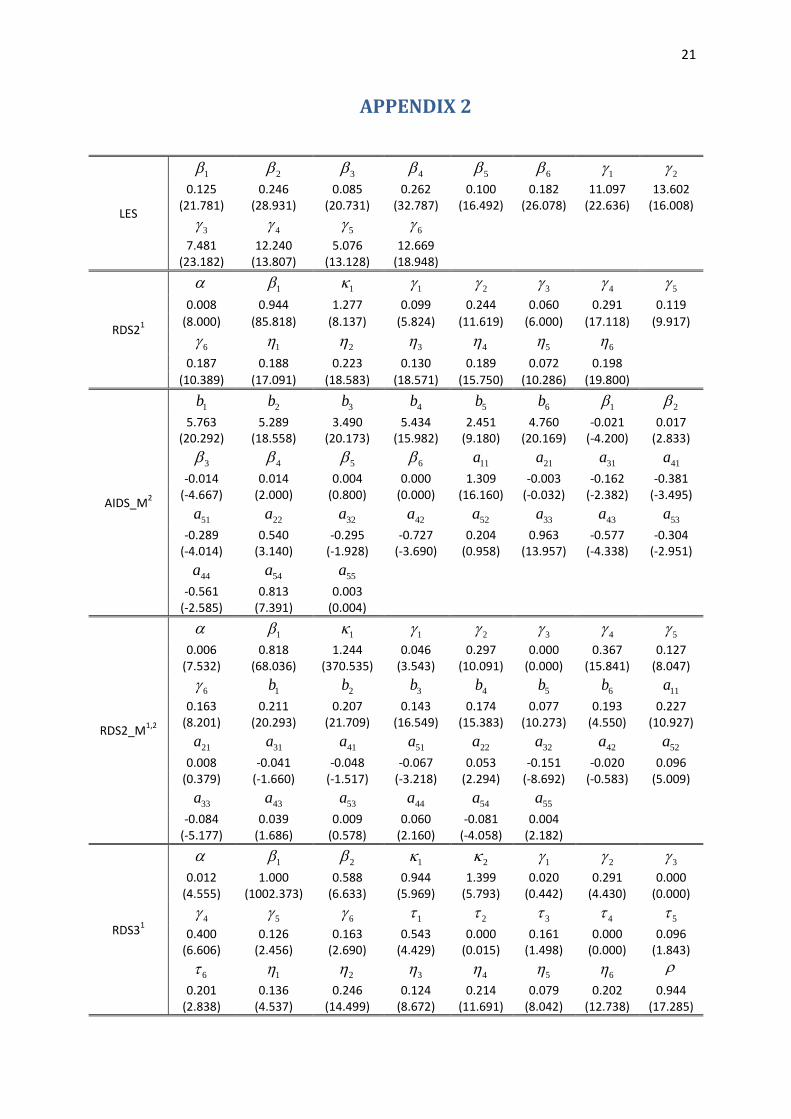
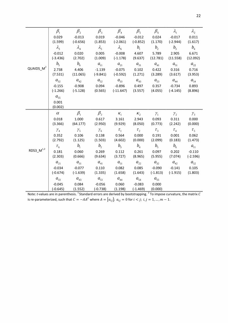
The likelihood estimates and corresponding t-values are summarized in Appendix 2. For

comparison, the AIC and BIC values for each model are presented in Table 1.

Table 1 AIC and BIC

Models AIC BIC

Ran

k 2

LES -13066.26 -13012.09

RDS2 -13112.97 -13048.95

AIDS_M -13122.09 -12998.98

RDS2_M -13152.45 -13014.56

Ran

k 3

RDS3 -13163.20 -13059.79

QUAIDS_M -13139.80 -12992.07

RDS3_M -13189.27 -13016.91

As shown in Table 1, the order in terms of AIC is: 1. RDS3_M; 2. RDS3; 3. RDS2_M; 4.

QUAIDS_M; 5. AIDS_M; 6. RDS2; 7. LES. It can be seen that the flexible rank-three model

RDS3_M performs better than its existing counterpart in the literature QUAIDS_M. The

flexible rank-two model RDS2_M outperforms its counterpart AIDS_M. One might have

thought that having more parameters, the existing flexible rank-three model QUAIDS_M

would have a stronger explanatory power than RDS3 which is globally regular but not fully

flexible in prices. However, it seems that the penalty of QUAIDS_M over-fitting apparently

outweighs the extra information that it might have achieved by increasing the number of

free parameters in the model. When free parameters are penalized more strongly, the order

in terms of BIC is: 1. RDS3; 2. RDS2; 3. RDS3_M; 4. RDS2_M; 5. LES; 6. AIDS_M; 7. QUAIDS_M.

According to this order, our rank-three globally regular model RDS3 performs the best, and

all the four examples of our class outperform the three existing alternatives. Therefore, to

sum up, this empirical evidence seems to favour global regularity over flexibility.

From Table 1, it can also be seen that moving from a rank-two system to a rank-three

system, for example from RDS3 to RDS2 or from RDS3_M to RDS2_M, which improves Engel

flexibility of a system, helps achieve a better performance in terms of AIC and BIC. This

evidence seems to imply that the true Engel curve might have a rank of three or higher. To

determine the rank, a more rigorous pre-specification rank test has to be implemented,

16

such as the nonparametric procedures proposed by Donald (1997) and Cragg and Donald

(1996), which is beyond the scope of this paper.

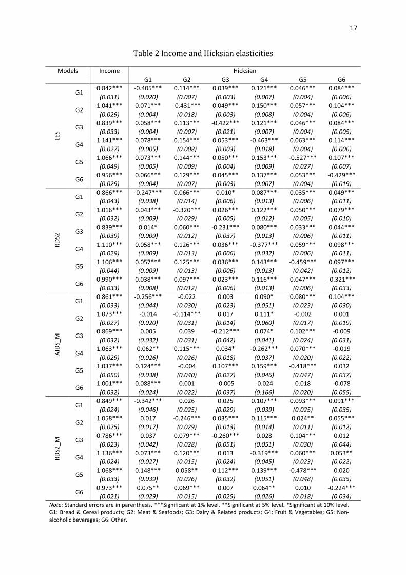
For illustration of elasticities, income and Hicksian elasticties are estimated for LES,

RDS2, AIDS_M and RDS2_M, all of which are rank-two demand systems, and are presented

in Table 2. Note that AIDS_M and RDS2_M are fully flexible in prices; in other words, they

possess enough parameters to attain arbitrary price elasticities at a point in price-

expenditure space.

As shown in Table 2, all the models produce similar estimates of income elasticities for

all the six goods, except that the income elasticity for the good “Other” is estimated slightly

above 1 by AIDS_M, which means “Other” is classified as a luxury good by AIDS_M, while

the others classify it as a necessity. Regarding price elasticities, all the four systems present

similar negative Hicksian own-price elasticities for all the six goods. As for Hicksian cross-

price elasticities, comparison between AIDS_M and RDS2_M, both of which are fully flexible

in prices and thus comparable, “Bread & Cereal products” and “Meats & Seafoods”, Non-

alcoholic beverages” and “Meats & Seafoods”, “Dairy & Related products” and “Other”, and

“Fruit & Vegetables” and “Other” are classified as complements by AIDS_M, while they are

classified as substitutes by RDS2_M. However, it is noteworthy that all these negative

estimates of the four cross-price elasticities by AIDS_M are not significant even at the 10%

significance level.

17

Table 2 Income and Hicksian elasticities

Models Income Hicksian

G1 G2 G3 G4 G5 G6

LES

G1 0.842*** -0.405*** 0.114*** 0.039*** 0.121*** 0.046*** 0.084***

(0.031) (0.020) (0.007) (0.003) (0.007) (0.004) (0.006)

G2 1.041*** 0.071*** -0.431*** 0.049*** 0.150*** 0.057*** 0.104***

(0.029) (0.004) (0.018) (0.003) (0.008) (0.004) (0.006)

G3 0.839*** 0.058*** 0.113*** -0.422*** 0.121*** 0.046*** 0.084***

(0.033) (0.004) (0.007) (0.021) (0.007) (0.004) (0.005)

G4 1.141*** 0.078*** 0.154*** 0.053*** -0.463*** 0.063*** 0.114***

(0.027) (0.005) (0.008) (0.003) (0.018) (0.004) (0.006)

G5 1.066*** 0.073*** 0.144*** 0.050*** 0.153*** -0.527*** 0.107***

(0.049) (0.005) (0.009) (0.004) (0.009) (0.027) (0.007)

G6 0.956*** 0.066*** 0.129*** 0.045*** 0.137*** 0.053*** -0.429***

(0.029) (0.004) (0.007) (0.003) (0.007) (0.004) (0.019)

RD

S2

G1 0.866*** -0.247*** 0.066*** 0.010* 0.087*** 0.035*** 0.049***

(0.043) (0.038) (0.014) (0.006) (0.013) (0.006) (0.011)

G2 1.016*** 0.043*** -0.320*** 0.026*** 0.122*** 0.050*** 0.079***

(0.032) (0.009) (0.029) (0.005) (0.012) (0.005) (0.010)

G3 0.839*** 0.014* 0.060*** -0.231*** 0.080*** 0.033*** 0.044***

(0.039) (0.009) (0.012) (0.037) (0.013) (0.006) (0.011)

G4 1.110*** 0.058*** 0.126*** 0.036*** -0.377*** 0.059*** 0.098***

(0.029) (0.009) (0.013) (0.006) (0.032) (0.006) (0.011)

G5 1.106*** 0.057*** 0.125*** 0.036*** 0.143*** -0.459*** 0.097***

(0.044) (0.009) (0.013) (0.006) (0.013) (0.042) (0.012)

G6 0.990*** 0.038*** 0.097*** 0.023*** 0.116*** 0.047*** -0.321***

(0.033) (0.008) (0.012) (0.006) (0.013) (0.006) (0.033)

AID

S_M

G1 0.861*** -0.256*** -0.022 0.003 0.090* 0.080*** 0.104***

(0.033) (0.044) (0.030) (0.023) (0.051) (0.023) (0.030)

G2 1.073*** -0.014 -0.114*** 0.017 0.111* -0.002 0.001

(0.027) (0.020) (0.031) (0.014) (0.060) (0.017) (0.019)

G3 0.869*** 0.005 0.039 -0.212*** 0.074* 0.102*** -0.009

(0.032) (0.032) (0.031) (0.042) (0.041) (0.024) (0.031)

G4 1.063*** 0.062** 0.115*** 0.034* -0.262*** 0.070*** -0.019

(0.029) (0.026) (0.026) (0.018) (0.037) (0.020) (0.022)

G5 1.037*** 0.124*** -0.004 0.107*** 0.159*** -0.418*** 0.032

(0.050) (0.038) (0.040) (0.027) (0.046) (0.047) (0.037)

G6 1.001*** 0.088*** 0.001 -0.005 -0.024 0.018 -0.078

(0.032) (0.024) (0.022) (0.037) (0.166) (0.020) (0.055)

RD

S2_M

G1 0.849*** -0.342*** 0.026 0.025 0.107*** 0.093*** 0.091***

(0.024) (0.046) (0.025) (0.029) (0.039) (0.025) (0.035)

G2 1.058*** 0.017 -0.246*** 0.035*** 0.115*** 0.024** 0.055***

(0.025) (0.017) (0.029) (0.013) (0.014) (0.011) (0.012)

G3 0.786*** 0.037 0.079*** -0.260*** 0.028 0.104*** 0.012

(0.023) (0.042) (0.028) (0.051) (0.051) (0.030) (0.044)

G4 1.136*** 0.073*** 0.120*** 0.013 -0.319*** 0.060*** 0.053**

(0.024) (0.027) (0.015) (0.024) (0.045) (0.023) (0.022)

G5 1.068*** 0.148*** 0.058** 0.112*** 0.139*** -0.478*** 0.020

(0.033) (0.039) (0.026) (0.032) (0.051) (0.048) (0.035)

G6 0.973*** 0.075** 0.069*** 0.007 0.064** 0.010 -0.224***

(0.021) (0.029) (0.015) (0.025) (0.026) (0.018) (0.034) Note: Standard errors are in parenthesis. ***Significant at 1% level. **Significant at 5% level. *Significant at 10% level. G1: Bread & Cereal products; G2: Meat & Seafoods; G3: Dairy & Related products; G4: Fruit & Vegetables; G5: Non-alcoholic beverages; G6: Other.

18

V. Conclusion

In this paper, we have introduced a new class of demand systems based on a simple

parametric specification of the indirect utility function, but allowing for the parsimonious

imposition of global regularity, i.e., fully consistent with the maximization of utility subject

to a budget constraint over the entire price-expenditure region. They also exhibit a clear and

reasonable homothetic asymptotic behaviour. In addition, this class of demand systems is

potentially fully flexible in rank, i.e., can acquire as large a rank as required for empirical

work. In an empirical application using Australian household expenditure data, according to

AIC and BIC, the four examples of this class outperform their popular existing counterparts

in the literature, and this empirical evidence therefore seems to favour global regularity

over flexibility.

Furthermore, income and Hicksian own- and cross-price elasticties are estimated for all

the rank-two demand systems illustrated in this study, namely LES, RDS2, AIDS_M and

RDS2_M, and are compared between each other. As a result, all these four systems produce

similar estimates for income elasticities and Hicksian own-price elasticities. As for Hicksian

cross-price elasticities, although four pairs of goods are classified as complements by

AIDS_M while classified as substitutes by RDS2_M, all the four negative estimates of cross-

price elasticities by AIDS_M are not significant even at the 10% significance level.

19

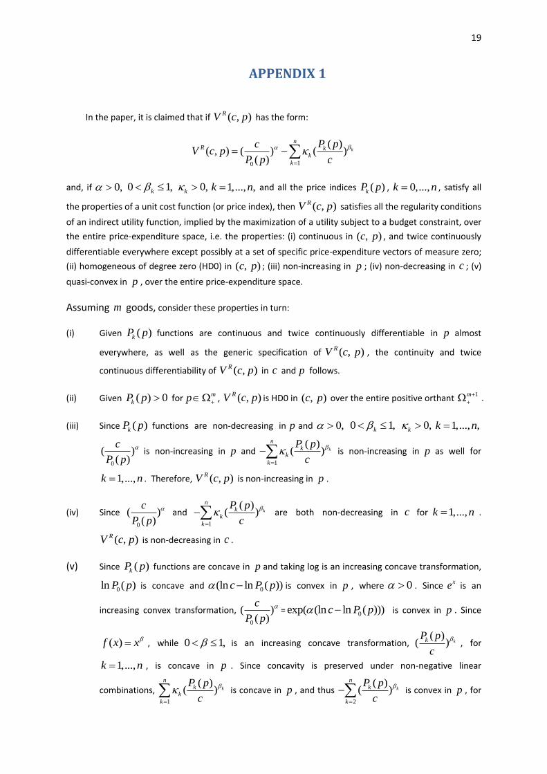
APPENDIX 1

In the paper, it is claimed that if ( , )RV c p has the form:

10

( )( , ) ( ) ( )

( )k

nR k

k

k

P pcV c p

P p c

and, if 0, 0 1,k 0,k 1,..., ,k n and all the price indices ( )kP p , 0,...,k n , satisfy all

the properties of a unit cost function (or price index), then ( , )RV c p satisfies all the regularity conditions

of an indirect utility function, implied by the maximization of a utility subject to a budget constraint, over

the entire price-expenditure space, i.e. the properties: (i) continuous in ( , )c p , and twice continuously

differentiable everywhere except possibly at a set of specific price-expenditure vectors of measure zero;

(ii) homogeneous of degree zero (HD0) in ( , )c p ; (iii) non-increasing in p ; (iv) non-decreasing in c ; (v)

quasi-convex in p , over the entire price-expenditure space.

Assuming m goods, consider these properties in turn:

(i) Given ( )kP p functions are continuous and twice continuously differentiable in p almost

everywhere, as well as the generic specification of ( , )RV c p , the continuity and twice

continuous differentiability of ( , )RV c p in c and p follows.

(ii) Given ( ) 0kP p for mp , ( , )RV c p is HD0 in ( , )c p over the entire positive orthant 1m

.

(iii) Since ( )kP p functions are non-decreasing in p and 0, 0 1,k 0,k 1,..., ,k n

0

( )( )

c

P p

is non-increasing in p and 1

( )( ) k

nk

k

k

P p

c

is non-increasing in p as well for

1,...,k n . Therefore, ( , )RV c p is non-increasing in p .

(iv) Since 0

( )( )

c

P p

and 1

( )( ) k

nk

k

k

P p

c

are both non-decreasing in c for 1,...,k n .

( , )RV c p is non-decreasing in c .

(v) Since ( )kP p functions are concave in p and taking log is an increasing concave transformation,

0ln ( )P p is concave and 0(ln ln ( ))c P p is convex in p , where 0 . Since xe is an

increasing convex transformation, 0

( )( )

c

P p

= 0exp( (ln ln ( )))c P p is convex in p . Since

( )f x x , while 0 1, is an increasing concave transformation, ( )

( ) kkP p

c

, for

1,...,k n , is concave in p . Since concavity is preserved under non-negative linear

combinations, 1

( )( ) k

nk

k

k

P p

c

is concave in p , and thus 2

( )( ) k

nk

k

P p

c

is convex in p , for

20

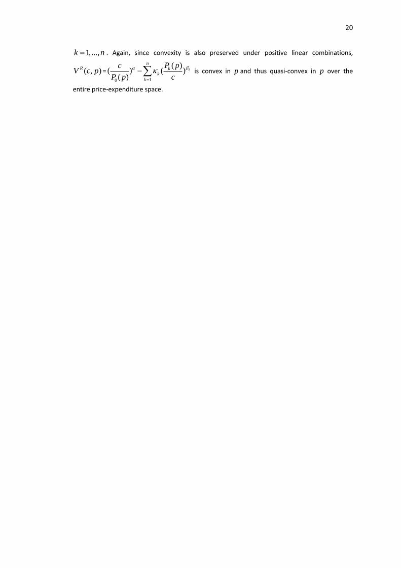
1,...,k n . Again, since convexity is also preserved under positive linear combinations,

( , )RV c p =10

( )( ) ( )

( )k

nk

k

k

P pc

P p c

is convex in p and thus quasi-convex in p over the

entire price-expenditure space.

21

APPENDIX 2

LES

1 2 3 4 5 6 1 2

0.125 0.246 0.085 0.262 0.100 0.182 11.097 13.602 (21.781) (28.931) (20.731) (32.787) (16.492) (26.078) (22.636) (16.008)

3 4 5 6

7.481 12.240 5.076 12.669 (23.182) (13.807) (13.128) (18.948)

RDS21

1 1 1 2 3 4 5

0.008 0.944 1.277 0.099 0.244 0.060 0.291 0.119

(8.000) (85.818) (8.137) (5.824) (11.619) (6.000) (17.118) (9.917)

6 1 2 3 4 5 6

0.187 0.188 0.223 0.130 0.189 0.072 0.198

(10.389) (17.091) (18.583) (18.571) (15.750) (10.286) (19.800)

AIDS_M2

1b 2b 3b 4b 5b 6b 1 2

5.763 5.289 3.490 5.434 2.451 4.760 -0.021 0.017 (20.292) (18.558) (20.173) (15.982) (9.180) (20.169) (-4.200) (2.833)

3 4 5 6 11a 21a 31a 41a

-0.014 0.014 0.004 0.000 1.309 -0.003 -0.162 -0.381 (-4.667) (2.000) (0.800) (0.000) (16.160) (-0.032) (-2.382) (-3.495)

51a 22a 32a 42a 52a 33a 43a 53a

-0.289 0.540 -0.295 -0.727 0.204 0.963 -0.577 -0.304 (-4.014) (3.140) (-1.928) (-3.690) (0.958) (13.957) (-4.338) (-2.951)

44a 54a 55a

-0.561 0.813 0.003 (-2.585) (7.391) (0.004)

RDS2_M1,2

1 1 1 2 3 4 5

0.006 0.818 1.244 0.046 0.297 0.000 0.367 0.127 (7.532) (68.036) (370.535) (3.543) (10.091) (0.000) (15.841) (8.047)

6 1b 2b 3b 4b 5b 6b 11a

0.163 0.211 0.207 0.143 0.174 0.077 0.193 0.227 (8.201) (20.293) (21.709) (16.549) (15.383) (10.273) (4.550) (10.927)

21a 31a 41a 51a 22a 32a 42a 52a

0.008 -0.041 -0.048 -0.067 0.053 -0.151 -0.020 0.096 (0.379) (-1.660) (-1.517) (-3.218) (2.294) (-8.692) (-0.583) (5.009)

33a 43a 53a 44a 54a 55a

-0.084 0.039 0.009 0.060 -0.081 0.004 (-5.177) (1.686) (0.578) (2.160) (-4.058) (2.182)

RDS31

1 2 1 2 1 2 3

0.012 1.000 0.588 0.944 1.399 0.020 0.291 0.000 (4.555) (1002.373) (6.633) (5.969) (5.793) (0.442) (4.430) (0.000)

4 5 6 1 2 3 4 5

0.400 0.126 0.163 0.543 0.000 0.161 0.000 0.096 (6.606) (2.456) (2.690) (4.429) (0.015) (1.498) (0.000) (1.843)

6 1 2 3 4 5 6

0.201 0.136 0.246 0.124 0.214 0.079 0.202 0.944 (2.838) (4.537) (14.499) (8.672) (11.691) (8.042) (12.738) (17.285)

22

QUAIDS_M2

1 2 3 4 5 6 1 2

0.029 -0.013 0.019 -0.046 -0.012 0.024 -0.017 0.011 (1.599) (-0.656) (1.853) (-2.061) (-0.852) (1.170) (-2.944) (1.617)

3 4 5 6 1b 2b 3b 4b

-0.012 0.020 0.005 -0.008 4.607 5.789 2.905 6.671 (-3.436) (2.702) (1.009) (-1.178) (9.637) (12.781) (11.558) (12.092)

5b 6b

11a 21a

31a 41a

51a 22a

2.738 4.406 -1.139 -0.075 0.102 0.422 0.316 0.716 (7.531) (11.065) (-9.841) (-0.592) (1.271) (3.289) (3.617) (3.953)

32a 42a 52a 33a 43a 53a 44a 54a

-0.155 -0.908 0.094 -0.896 0.497 0.357 -0.734 0.893 (-1.266) (-5.128) (0.565) (-11.647) (3.557) (4.055) (-4.145) (8.896)

55a

0.001 (0.002)

RDS3_M1,2

1 2 1 2 1 2 3

0.018 1.000 0.617 3.161 2.943 0.093 0.311 0.000 (3.366) (64.177) (2.950) (9.929) (8.050) (0.773) (2.242) (0.000)

4 5 6 1 2 3 4 5

0.352 0.106 0.138 0.564 0.000 0.191 0.001 0.062 (2.792) (1.125) (1.503) (4.602) (0.000) (2.099) (0.183) (1.473)

6 1b 2b 3b 4b 5b 6b 11a

0.181 0.060 0.269 0.112 0.261 0.097 0.202 -0.110 (2.303) (0.666) (9.634) (3.727) (8.965) (5.955) (7.074) (-2.596)

21a 31a 41a 51a 22a 32a 42a 52a

-0.034 -0.077 0.110 0.082 0.085 -0.090 -0.141 0.105 (-0.674) (-1.639) (1.335) (1.658) (1.643) (-1.813) (-1.915) (1.803)

33a 43a 53a 44a 54a 55a

-0.045 0.084 -0.056 0.060 -0.083 0.000 (-0.645) (1.552) (-0.738) (1.198) (-1.469) (0.000)

Note: t-values are in parenthesis. 1 Standard errors are derived by bootstrapping. 2 To impose curvature, the matrix

is re-parameterized, such that where [ ] for .

23

References

Banks, J., R. Blundell, and A. Lewbel. 1997. “Quadratic Engel Curves and Consumer Demand.” Review of Economics and Statistics 79 (4): 527–539.

Barnett, W. A., and A. Jonas. 1983. “The Muntz-Szatz Demand System : An Application of a Globally Well Behaved Series Expansion.” Economics Letters 11 (4): 337–342.

Barnett, W.A. 1983. “New Indices of Money Supply and the Flexible Laurent Demand System.” Journal of Business & Economic Statistics 1 (1): 723.

———. 1985. “The Minflex-Laurent Translog Flexible Functional Form.” Journal of Econometrics 30 (1): 33–44.

———. 2002. “Tastes and Technology: Curvature Is Not Sufficient for Regularity.” Journal of Econometrics 108 (1): 199–202.

Barnett, W.A., and Y.W. Lee. 1985. “The Global Properties of the Minflex Laurent, Generalized Leontief, and Translog Flexible Functional Forms.” Econometrica 53 (6): 1421–1437.

Barnett, W.A., and P. Yue. 1988. “Semiparametric Estimation of the Asymptotically Ideal Model: The AIM Demand System.” In George Rhodes and Thomas Fomby (eds.), Nonparametric and Robust Inference, Advances in Econometrics 7, 229–252.

Barten, A.P. 1966. “Theorie En Empirie van Een Volledig Stelsel van Vraegvergelijkingen”. University of Rotterdam.

Byrd, R. H., P. Lu, J. Nocedal, and C. Zhu. 1995. “A Limited Memory Algorithm for Bound Constrained Optimization.” SIAM J. Scientific Computing 16 (5): 1190–1208.

Christensen, L.R., D.W. Jorgenson, and L.J. Lau. 1975. “Transcendental Logarithmic Utility Functions.” The American Economic Review 65 (3): 367–383.

Cooper, R.J., and K.R. McLaren. 1992. “An Empirically Oriented Demand System with Improved Regularity Properties.” Canadian Journal of Economics 25 (3): 652–668.

———. 1996. “A System of Demand Equations Satisfying Effectively Global Regularity Conditions.” The Review of Economics and Statistics 78 (2): 359–364.

———. 2006. “Demand Systems Based on Regular Ratio Indirect Utility Functions.” In ESAM06.

Cooper, R.J., K.R. McLaren, and P. Parameswaran. 1994. “A System of Demand Equations Satisfying Effectively Global Curvature Conditions.” Economic Record 70 (208): 26–35.

24

Cragg, J.G., and S.G. Donald. 1996. “On the Asymptotic Properties of LDU-based Tests of the Rank of a Matrix.” Journal of the American Statistical Association 91 (435): 1301–1309.

Deaton, A. 1987. “Estimation of Own- and Cross-price Elasticities from Household Survey Data.” Journal of Econometrics 36 (1-2): 7–30.

———. 1988. “Quality, Quantity, and Spatial Variation of Price.” The American Economic Review 78 (3): 418–430.

Deaton, A., and J. Muellbauer. 1980a. Economics and Consumer Behavior. Cambridge; New York: Cambridge University Press.

———. 1980b. “An Almost Ideal Demand System.” American Economic Review 70 (3): 312–326.

Diewert, W.E. 1971. “An Application of the Shephard Duality Theorem: a Generalized Leontief Production Function.” The Journal of Political Economy 79 (3): 481–507.

———. 1974. “Applications of Duality Theory.” In Frontiers of Quantitative Economics, Vol. 2, edited by Michael D. Intriligator and David A. Kendrick, Ch.3. Amsterdam.

———. 1982. “Chapter 12 Duality Approaches to Microeconomic Theory.” In: Kenneth

J. Arrow and Michael D. Intriligator, Editor(s), Handbook of Mathematical Economics,

Elsevier, Vol. 2: 535–599.

Diewert, W.E., and T.J. Wales. 1987. “Flexible Functional Forms and Global Curvature Conditions.” Econometrica 55 (1): 43–69.

Donald, S.G. 1997. “Inference Concerning the Number of Factors in a Multivariate Nonparametric Relationship.” Econometrica 65 (1): 103–131.

Dong, D., B.W. Gould, and H.M. Kaiser. 2004. “Food Demand in Mexico: An Application of the Amemiya-Tobin Approach to the Estimation of a Censored Food System.” American Journal of Agricultural Economics 86 (4): 1094–107.

Elbadawi, I., A.R. Gallant, and G. Souza. 1983. “An Elasticity Can Be Estimated Consistently Without a Priori Knowledge of Functional Form.” Econometrica 51 (6): 1731–1751.

Gallant, A.R. 1981. “On the Bias in Flexible Functional Forms and an Essentially Unbiased Form: The Fourier Flexible Form.” Journal of Econometrics 15 (2): 211–245.

———. 1984. “The Fourier Flexible Form.” American Journal of Agricultural Economics 66 (2): 204–208.

Gallant, A.R., and G.H. Golub. 1984. “Imposing Curvature Restrictions on Flexible Functional Forms.” Journal of Econometrics 26 (3): 295–321.

25

Heien, D, and C.R. Wessells. 1990. “Demand Systems Estimation with Microdata: a Censored Regression Approach.” Journal of Business & Economic Statistics 8 (3): 365–371.

Hoderlein, S., and S. Mihaleva. 2008. “Increasing the Price Variation in a Repeated Cross Section.” Journal of Econometrics 147 (2): 316–325.

Lau, L.J. 1986. “Functional Forms in Econometric Model Building.” Handbook of Econometrics 3: 1515–1566.

Lewbel, A. 1987. “Fractional Demand Systems.” Journal of Econometrics 36 (3): 311–337.

———. 1989. “Identification and Estimation of Equivalence Scales Under Weak Separability.” The Review of Economic Studies 56 (2): 311–316.

———. 1991. “The Rank of Demand Systems: Theory and Nonparametric Estimation.” Econometrica 59 (3): 711–730.

———. 2003. “A Rational Rank Four Demand System.” Journal of Applied Econometrics 18 (2) (March): 127–135.

McLaren, K.R., and K.K. Wong. 2009. “Effective Global Regularity and Empirical Modelling of Direct, Inverse, and Mixed Demand Systems.” Canadian Journal of Economics 42 (2): 749–770.

Meyerhoefer, C.D., C.K. Ranney, and D.E. Sahn. 2005. “Consistent Estimation of Censored Demand Systems Using Panel Data.” American Journal of Agricultural Economics 87 (3): 660–672.

Muellbauer, J. 1975. “Aggregation, Income Distribution and Consumer Demand.” The Review of Economic Studies 42 (4): 525–543.

Pollak, R. A., and T. J. Wales. 1992. Demand System Specification and Estimation. Oxford University Press.

Sam, A.G., and Y. Zheng. 2010. “Semiparametric Estimation of Consumer Demand Systems with Micro Data.” American Journal of Agricultural Economics 92 (1): 246.

Shonkwiler, J.S., and S.T. Yen. 1999. “Two-Step Estimation of a Censored System of Equations.” American Journal of Agricultural Economics 81 (4): 972–982.

Stone, R. 1954. The Measurement of Consumers’ Expenditure and Behaviour in the United Kingdom, 1920-1938, Volume 1. Cambridge University Press.

Theil, H. 1965. “The Information Approach to Demand Analysis.” Econometrica 33 (1): 67–87.

26

Wiley, D.E., W.H. Schmidt, and W.J. Bramble. 1973. “Studies of a Class of Covariance Structure Models.” Journal of the American Statistical Association 68 (342): 317–323.

Yen, S.T., B.H. Lin, and D.M. Smallwood. 2003. “Quasi-and Simulated-Likelihood Approaches to Censored Demand Systems: Food Consumption by Food Stamp Recipients in the United States.” American Journal of Agricultural Economics 85 (2): 458–478.