Carvajal Microeconomic Theory

EC901 MICROECONOMIC THEORY

(For teaching only - Do not cite)

Andres Carvajal 1

Fall term, 2008 - 09

1E-mail address: [email protected].

1 CONSUMER THEORY

Human beings are complicated objects, and human behavior is difficult to model.

Here we consider the problem of a decision-maker who has to choose a bundle of

commodities, subject to a budgetary constraint. The decision-maker could be a per-

son, or a group of people (for instance a family); for simplicity we will treat the

decision-maker as a person. In order to make this problem tractable, we will ab-

stract from the problems of what commodities are available (we take them as given),

and will model the person through two elements: what she wants, and what she can

do.

1.1 CONSUMPTION SPACE AND PREFERENCES

We consider a situation in which a person is to choose a bundle of L commodities.

These commodities are perfectly divisible and can be consumed in any nonnegative

amount: the consumption set is the nonnegative orthant RL+, so a bundle of commodi-

ties is x = (x1, . . . , xL), where each xl represents the number of units of commodity

l that make part of the bundle. We take the facts that these commodities exist as

exogenous.

The first element in our model of the person is what she wants. For us, the indi-

vidual’s preferences are subjective judgments about the relative desirability of bun-

dles: given two bundles, preferences are defined by her answer to the question ‘is the

first bundle at least as good as the second one? Formally, then, the decision-maker’s

preferences are a binary relation % defined on the consumption set: given a pair of

commodity bundles x and x′, we write x % x′ if, according to the person’s tastes,

x is at least as good as x′.1 We also take the person’s preferences as exogenous, in

the sense that we do not explain where they come from. Instead, we concentrate on

the problem of studying the individual’s behavior given her preferences, under the

assumption that these preferences will not be affected by the person’s choices.

We start by studying properties that the individual’s preferences may (but need

not) satisfy. We first study properties of a binary relation under which it makes sense

to identify this relation with someone’s preferences.

DEFINITION. We say that a binary relation % is

1. complete if for any x and any x′, either x % x′ or x′ % x;

1 Formally, % can be seen as a subset of RL+ × RL

+.

1

2. reflexive if for any x, x % x;

3. transitive if x % x′ and x′ % x′′ imply x % x′′; and

4. rational if it is complete, reflexive and transitive.

Consumers with incomplete preferences may find instances in which they are un-

able to choose: they are simply unable to make a value judgments about the relative

(subjective) quality of two bundle. Reflexivity is consistent with our interpretation

of ‘weak’ preference. Consumers with nontransitive preferences are open to full rent

extraction, as a person could find a cycle of bundles for which the person is willing

to pay a positive premium at each step. In economics, one usually assumes that the

decision-maker under consideration has rational preferences, although in some cases

(e.g. very complicated problems) it may be reasonable to consider that in individual’s

preferences are incomplete; also, some cases of nontransitive preferences are some-

times observed in real life. In any case, from now on, we fix a rational binary relation

%, and define the following (induced) binary relations on the consumption set: (i)

the strict preference relation �, by saying x � x′ if it is not true that x′ % x; and the

indifference relation ∼, by saying x ∼ x′ if it is true that x % x′ and that x′ % x.

EXERCISE 1.1. Argue that � is transitive, but not reflexive, and that ∼ is reflexive and

transitive. Could these relations be complete? Could they be rational?

A second set of properties studies whether our consumer “likes” the commodities

available, in the sense that the more she consumes them the happier she is.


1. strictly monotone if x > x′ implies x � x′;

2. monotone if x� x′ implies x � x′;

3. locally nonsatiated if for every x and every ε > 0, one can find x′ with ||x − x′|| < ε

and x′ � x.

The first property captures the case when all goods, one by one, are good for the

individual: with strictly monotone preferences, getting more of any one commodity

improves the bundle. With monotone preferences, getting more of all commodities

improves the bundle. Local nonsatiation does not capture that the commodities are

2

good,2 but it implies that the individual will not have bliss points, in the sense that

any bundle can be improved, even with a small perturbation. In particular, the as-

sumption of locally nonsatiated preferences rules out thick indifference curves.

EXERCISE 1.2. Argue that strict monotonicity implies monotonicity and that monotonicity

implies local nonsatiation. Does monotonicity imply strict monotonicity? Does local non-

satiation imply monotonicity or strict monotonicity? Does strict monotonicity imply local

nonsatiation?

A third group of properties studies whether our consumer likes to ‘combine’ com-

modities in bundles.


1. convex if for any bundle x, any bundle x′ such that x % x′, and any scalar 0 ≤ α ≤ 1,

it is true that αx+ (1− α)x′ % x′;

2. strongly convex if for any bundle x, any bundle x′ 6= x such that x % x′, and any

scalar 0 < α < 1, it is true that αx+ (1− α)x′ � x′.

Convex preferences favor “balanced” bundles, in the sense that if the individual

has two bundles that have different composition but make her equally happy, then

she would not be worse off with a third bundle that just combined (took an average)

of them . Strongly convex preferences do too, in a strong sense: if the two original

bundles were different, then the combination is considered to be strictly better by

the consumer. The indifference map of a convex binary relation has the usual shape,

whereas if the relation is strongly convex, then its indifference curves cannot have

straight portions.

EXERCISE 1.3. Argue that strong convexity implies convexity. Does convexity imply strong

convexity?

It is most usual in economics to represent a decision-maker’s preferences by a

function that gives a higher value the more the person likes a bundle.


1. represented by function u : RL+ → R if u(x) ≥ u(x′) occurs if, and only if, x % x′;

2 Except in the very weak sense that it cannot be that not getting anything of any commodity is the

best that can happen to the consumer

3

2. representable if there is some u : RL+ → R that represents it.

The function u that represents% is called “utility function.” Notice that if a prefer-

ence relation is representable, then there are infinitely many different utility functions

that represent it. All these representations will have the same contour sets (i.e. the

same ordinal information), but may give nontrivially different utility levels (i.e. dif-

ferent cardinal information). It is for this reason that interpersonal comparisons of

utility are problematic.

EXERCISE 1.4. Argue that representability implies rationality. Does rationality imply repre-

sentability? What property must u satisfy if it represents a convex %? What property must u

satisfy if it represents a monotone %?

1.2 PREFERENCE MAXIMIZATION: MARSHALLIAN DEMAND

We now study the consumer’s behavior when deciding a consumption bundle. The

second element in the formalization of this behavior is the definition of what bun-

dles are available for the person to choose. Here, we adopt the competitive setting:

a price is given for each commodity, and the consumer has a nominal wealth that

she can spend in her bundle. Both of these variables are here considered to be ex-

ogenous; later, when studying general equilibrium, we will endogenize them. For-

mally, let us fix some rational preferences %, a vector of prices for all commodities

p = (p1, . . . , pL) � 0 and nominal income m ≥ 0. The preference maximization prob-

lem is to find x that (i) is affordable: p · x ≤ m; and (ii) cannot be improved upon:

for every other x′ that is affordable (i.e. such that p · x′ ≤ m), it is true that x % x′.

In consumer theory, we will assume that a (competitive) consumer behaves as if she

solved the problem above.

The most immediate questions are whether this problem has solutions and, if so,

how many. The problem of existence of solution is somewhat technical, so we’ll skew

it: suffice it to say that when preferences are such that they don’t change abruptly

as one changes consumption (e.g. if they can be represented by a continuous utility

function), the problem has a solution. From now on, let us assume that a solution

exists. Notice that if preferences are strongly convex, the solution is unique. From

now on, let us assume that % is strongly convex and denote by x(p,m) the unique

solution to this problem. As we vary prices and income, the preference maximization

problem defines an “optimal demand” function x : RL++×R+ → RL

+, which is known

as the Marshallian demand function.

4

1.2.1 PROPERTIES OF THE MARSHALLIAN DEMAND

PROPOSITION 1.1. The following are properties of the Marshallian demand, under our as-

sumptions on %:

1. Homogeneity of degree zero: for any (p,m) and any α > 0, it is true that x(αp, αm) =

x(p,m);

2. Walras’s law: if % is locally nonsatiated, then the consumer spends all her nominal

income: for any (p,m), p · x(p,m) = m;

3. Weak Axiom of Revealed Preferences (WARP): for any (p,m) and any (p′,m′), if p ·x(p′,m′) ≤ m and p′ ·x(p,m) ≤ m′, then it must also be true that x(p,m) = x(p′,m′).

EXERCISE 1.5. Let L = 2, and suppose an agent who spends all her money, but who may or

may not be rational.

1. Suppose that at p = (1, 1) she demands x = (1, 1). Suppose that at prices p′ = (2, 3)

and income m′ = 4 her demand, x′ = (x′1, x′2), is unknown. For what values of x′1

would she violate WARP?

2. Suppose that at p = (10, 10) she demands x = (1, 1). Suppose that at prices p′ = (10, 8)

and income m′ her demand is x′ = (65, x′2), where both m′ and x′2 are unknown. For

what values of x′2 would she violate WARP?

1.2.2 THE INDIRECT UTILITY FUNCTION

Under representability of preferences, we can simply write that x(p,m) solves maxx u(x) :

p · x ≤ m. The “value” function, v(p,m) = u(x(p,m)) is known as the Indirect Utility

function.3

PROPOSITION 1.2. The following are properties of the indirect utility function:

1. Homogeneity of degree zero: for any (p,m) and any α > 0, v(αp, αm) = v(p,m);

2. If % is locally nonsatiated, then v is increasing in m and nonincreasing in p: (i) if

m > m′, then, for any p, v(p,m) > v(p,m′); and if p ≥ p′, then, for any m, v(p,m) ≤v(p′,m).

3. Quasiconvexity: if (p,m) and (p′,m′) are such that v(p,m) ≥ v(p′,m′) and 0 ≤ α ≤ 1,

then it must be true that

v(αp+ (1− α)p′, αm+ (1− α)m′) ≤ v(p,m).

3 We should simply write v(p,m) = maxx u(x) : p · x ≤ m.

5

1.2.3 DIFFERENTIABLE CONSUMER

Suppose furthermore that u is twice continuously differentiable4 and has interior con-

tours.5 Suppose that u is strictly monotone and strongly quasiconcave,6 and consider

only m > 0.

PROPOSITION 1.3. Under the assumptions stated above,

1. Marshallian demand is interior: for any (p,m), x(p,m)� 0;

2. For given (p,m), bundle x(p,m) is the only x for which there exists λ > 0 such that

Du(x) = λp and p · x = m;

3. The Marshallian demand function x is differentiable;

4. The indirect utility function, v, is differentiable, and the marginal utility is given by

∂mv(p,m) = λ(p,m) = 1p1∂x1u(x(p,m)).

Moreover, the following properties are important restrictions in applied work:

PROPOSITION 1.4. Under the assumptions stated above, the following are properties of the

Marshallian demands, at all (p,m):

1. Cournot aggregation: for any commodity l′,

xl′(p,m) +∑l

pl∂pl′xl(p,m) = 0;

2. Engle aggregation:∑

l pl∂mxl(p,m) = 1;

3. Euler aggregation: for any l′,∑

l pl∂plxl′(p,m) +m∂mxl′(p,m) = 0.

And the following property of the indirect utility function is very useful in theo-

retical work:

PROPOSITION 1.5 (Roy’s identity). Under the assumptions stated above, for any commod-

ity l′ we have that

−∂pl′v(p,m)

∂mv(p,m)= xl′(p,m).

4 The following notation will be used: for any function f(x, y), the partial derivative with respect

to x will be denoted by ∂xf(x, y); the gradient of any function f(x) will be denoted by Df(x) and its

Hessian will be D2f(x).5 That is, that for every x ∈ RL

++, it is true that {x′|u(x′) ≥ u(x)} ⊆ RL++.

6 In this setting, we are assuming that, whenever x � 0, it is true that Du(x) � 0 and that

δTD2u(x)δ < 0 for any δ 6= 0 such that δ ·Du(x) = 0.

6

Proof: A direct proof can be given by the Envelope theorem. Alternatively, recall that

v(p,m) = u(x(p,m)). Then, differentiating with respect to pl′ , by the chain rule,

∂pl′v(p,m) =∑l

∂xlu(x(p,m))∂pl′xl(p,m).

By the first order conditions (Proposition 1.3), we can substitute ∂xlu(x(p,m)) = λ(p,m)pl,

to get

∂pl′v(p,m) = λ(p,m)∑l

pl∂pl′xl(p,m) = −λ(p,m)xl′(p,m),

where the second equality comes from Cournot aggregation (Proposition 1.4). Simi-

larly, but using Engle aggregation,7

∂mv(p,m) =∑l

∂xlu(x(p,m))∂mxl(p,m)

= λ(p,m)∑l

pl∂mxl(p,m)

= λ(p,m).

Q.E.D.

EXERCISE 1.6. Suppose that L = 2, and consider a consumer whose preferences are repre-

sented by

u(x) = α ln(x1) + (1− α) ln(x2),

for 0 < α < 1. Are the preferences of this consumer rational? Are they locally nonsatiated?

Are they convex? Find the Marshallian demand and the indirect utility functions? Verify

homogeneity of degree zero of both functions. Verify Walras’s law. Verify that the indirect

utility is increasing in income and nonincreasing in prices. Verify differentiability. Verify the

conditions of aggregation of Cournot, Engel and Euler. Verify Roy’s identity.

1.3 EXPENDITURE MINIMIZATION: HICKSIAN DEMAND

Fix rational, strongly convex preferences %. Suppose that a continuous utility func-

tion u represents %.

For prices p� 0 and a feasible utility level υ, the expenditure minimization prob-

lem is to find x such that: (i) it gives utility at least equal to υ: u(x) ≥ υ; and (ii) for

every other x′ such that u(x′) ≥ υ, it is true that p · x′ ≥ p · x. That is, to find x that

solves minx p · x : u(x) ≥ υ.7 The equations that follow prove the last statement in Proposition 1.3.

7

Under our assumptions, the problem is guaranteed to have a unique solution,

which we denote by h(p, υ). Function h : RL++ × u[RL

+]→ RL+ is known as the Hicksian

demand function.8

1.3.1 PROPERTIES OF THE HICKSIAN DEMAND

PROPOSITION 1.6. The following are properties of the Hicksian demand, under our assump-

tions on %:

1. Homogeneity of degree zero in p: for any (p, υ) and any α > 0, it is true that h(αp, υ) =

h(p, υ).

2. No excess utility: for any (p, υ), it is true that u(h(p, υ)) = υ.

3. The compensated law of demand: for any p and p′, and any υ, it is true that

(p− p′) · (h(p, υ)− h(p′, υ)) ≤ 0.

Proof: We only proof the compesated law of demand. Notice that, by definition,

p · h(p, υ) ≤ p · h(p′, υ) and p′ · h(p′, υ) ≤ p′ · h(p, υ). Immediately,

p · h(p, υ) + p′ · h(p′, υ) ≤ p · h(p′, υ) + p′ · h(p, υ).

Q.E.D.

Notice that there is no analogous of the last property that holds true for the Mar-

shallian demand!

EXERCISE 1.7. For the consumer considered in Exercise 1.6, find the Hicksian demand func-

tion. Verify homogeneity of degree zero in p, no excess utility and the compensated law of

demand.

1.3.2 THE EXPENDITURE FUNCTION

The value function of the expenditure minimization problem is the Expenditure Func-

tion: e : RL++ × u[RL

+]→ R+, defined by e(p, υ) = p · h(p, υ).9

PROPOSITION 1.7. The following are properties of the expenditure function:

8 Here, u[RL+] denotes the set of feasible utility levels: u[RL

+] = {υ ∈ R|∃x ∈ RL+ : u(x) = υ}.

9 Or, e(p, υ) = minx p · x : u(x) ≥ υ.

8

1. Homogeneity of degree one in p: for any (p, υ) and any α > 0, e(αp, υ) = αe(p, υ).

2. If preferences are monotonic, then e is increasing in υ and nondecreasing in p: if υ > υ′,

then, for any p, it is true that e(p, υ) > e(p, υ′); and if p ≥ p′, then, for any υ, it is true

that e(p, υ) ≥ e(p′, υ).

3. Concavity in p: for any p, p′ and υ and any 0 ≤ α ≤ 1, it is true that

e(αp+ (1− α)p′, υ) ≥ αe(p, υ) + (1− α)e(p′, υ).

Proof: We prove only concavity in p. Notice that, by definition, e(p, υ) ≤ p · h(αp +

(1− α)p′, υ) and e(p′, υ) ≤ p′ · h(αp+ (1− α)p′, υ). Then, taking the average,

αe(p, υ) + (1− α)e(p′, υ) ≤ (αp+ (1− α)p′) · h(αp+ (1− α)p′, υ).

Q.E.D.

Notice that the last property is cardinal, while the analogous result for in the indi-

rect utility function is only ordinal!

1.3.3 DIFFERENTIABLE CONSUMER

Suppose again that the utility function u representing the consumer’s preferences is

(twice continuously) differentiable and has interior indifference curves. Suppose also

that u is strictly monotone and strongly quasiconcave.

PROPOSITION 1.8. Under the assumptions stated above, and considering only interior utility

levels υ > u(0), the following is true:

1. Hicksian demand is interior: for any (p, υ), h(p, υ)� 0.

2. For given (p, υ), bundle h(p, υ) is the only x for which there exists γ > 0 such that

p = γDu(x) and u(x) = υ.

3. The Hicksian demand function, h, is differentiable;

4. The expenditure function, e, is differentiable, and the marginal expenditure is given by

∂υe(p, υ) = γ(p, υ) = (∂x1u(x(p, υ)))−1p1.

Furthermore, the following restrictions are important in applied and theoretical

work:

9

PROPOSITION 1.9. Under the assumptions stated above, and considering only interior utility

levels υ > u(0),the following is true:

1. Negative semidefiniteness: for any p and υ, matrix D2p,pe(p, υ) is negative semidefinite;

2. Shephard’s lemma: for any commodity l′, ∂pl′e(p, υ) = hl′(p, υ);

3. Symmetry and negative-semidefiniteness of substitution effects: matrix Dph(p, υ) is

symmetric and negative semidefinite.

Proof: Negative semidefiniteness of D2p,pe(p, υ) is immediate from the fact that e is

concave (Proposition 1.8).

For Shephard’s lemma, notice first that, by no excess utility (Proposition 1.6),

u(h(p, υ)) = υ. Then, taking derivatives,∑l

∂xlu(h(p, υ))∂pl′hl(p, υ) = 0.

By first-order conditions (Proposition 1.8), we can substitute ∂xlu(h(p, υ) = 1γ(p,υ)

pl, to

get that∑

l pl∂pl′hl(p, υ) = 0. Now, recall that e(p, υ) = p · h(p, υ), so, differentiating,

∂pl′e(p, υ) = hl′(p, υ) +∑l

pl∂pl′hl(p, υ) = hl′(p, υ).

Shephard’s lemma immediately implies that Dph(p, υ) = D2p,pe(p, υ), so negative

semidefiniteness follows from part 1, while symmetry follows from a well-known re-

sult in mathematics, Young’s Theorem. Q.E.D.

Symmetry of Dph(p, υ) is an example of a result that was discovered after the

application of mathematics, but was not anticipated by intuitive arguments.

EXERCISE 1.8. For the same consumer as in Exercise 1.6, verify that e is increasing in p and

in υ. Verify that e is homogeneous of degree one and concave in p. Verify Shephard’s lemma.

1.4 DUALITY

For the purposes of this section, fix rational, strongly convex, locally nonsatiated pref-

erences %, and let the utility function u represent %.

PROPOSITION 1.10 (Duality Theorem). Fix prices p� 0, nominal incomem and a feasible

utility level υ. Under the assumptions above, the following is true:

10

1. Marsallian demand at income equal to minimized expenditure is the same as Hicksian

demand: x(p, e(p, υ)) = h(p, υ);

2. Hicksian demand at utility level equal to maximized utility is the same as Marshallian

demand: h(p, v(p,m)) = x(p,m);

3. Maximized utility at income equal to minimized expenditure is the same as required

utility: v(p, e(p, υ)) = υ;

4. Minimized expenditure at utility level equal to maximized utility is the same as nominal

income: e(p, v(p,m)) = m.

Proof: For part 1, suppose that the equality does not hold. Since p ·h(p, υ) = e(p, υ), it

must be that u(x(p, e(p, υ))) > u(h(p, υ)) = υ. But then, since p · x(p, e(p, υ)) ≤ e(p, υ),

we have that x(p, e(p, υ)) solves the expenditure minimization problem too, which

would violate “no excess utility” (Proposition 1.6).

For part 2, again suppose otherwise. Since u(x(p,m)) = v(p,m), it must be that

p · h(p, v(p,m)) < p · x(p,m) = m. But then, since u(h(p, v(p,m)) ≥ v(p,m), we have

that h(p, v(p,m)) solves the utility maximization problem too, which would violate

Walras’s law (Proposition 1.1).

Part 3 is immediate from part 1, given no excess utility, and part 4 follows from

part 2, given Walras’s law. Q.E.D.

The Duality Theorem allows us to go from one problem to the other without need-

ing to solve them both. Notice that the assumption that p� 0 is crucial. For instance,

if p = 0, then any bundle with u(x) ≥ υ solves the expenditure minimization problem

(and at least one such bundle exists), whereas the utility maximization problem has

no solution, given that preferences are locally nonsatiated.

EXERCISE 1.9. For the same consumer as in Exercise 1.6, verify the duality equalities.

When the utility function u is twice continuously differentiable and has interior

indifference curves, one has the following crucial result.

PROPOSITION 1.11 (Slutsky’s Identity). Suppose that u is strictly monotone and strongly

quasiconcave. Fix a feasible utility level υ and define a nominal income m = e(p, υ). Then,

for each pair of commodities l and l′, the following is true:

∂pl′xl(p,m) = ∂pl′hl(p, υ)− xl′(p,m)∂mxl(p,m).

11

Proof: From the Duality Theorem (Proposition 1.10), we know that xl(p, e(p, υ)) =

hl(p, υ). Then, differentiating,

∂pl′xl(p, e(p, υ)) + ∂mxl(p, e(p, υ))∂pl′e(p, υ) = ∂pl′hl(p, υ).

By Shephard’s Lemma (Proposition 1.9) and duality, we can substitute ∂pl′e(p, υ) =

hl′(p, υ) = xl′(p, e(p, υ)). The result follows since m = e(p, υ). Q.E.D.

EXERCISE 1.10. For the same consumer as in exercise 1.6, verify the duality equalities and

Slutsky’s identity.

Letting the substitution matrix be S(p,m) = Dph(p, v(p,m)), Slutsky’s Identity

writes in matrix terms as Dpx(p,m) = S(p,m) −Dmx(p,m)x(p,m)T. That the substi-

tution matrix is symmetric and negative semidefinite is a necessary condition implied

by rationality of the consumer. Another necessary condition is that the matrix should

have (exactly)L−1 of its columns linearly independent. Remarkably, these conditions

are also sufficient for rationality!

1.5 ADDITIONAL EXERCISES

EXERCISE 1.11. Consider a standard consumer with preferences %, over nonnegative con-

sumption of two commodities, represented by u(x) = x1 + ln(x2). Answer and solve:

1. Are these preferences rational? Are they convex? Are they strongly convex? Are they

monotone? Are they strictly monotone?

2. Find Marshallian demands and the indirect utility function. Verify Roy’s identity.

(Warning: be careful about the nonnegativity constraint!)

3. Find the expenditure function and the Hicksian demands.

EXERCISE 1.12. For a consumer in a two-commodity world, solve:

1. Suppose that the following information is known: when her income is m = 5 and prices

are p = (1, 1), her demand of commodity 1 is x1 = 3; when her income is m′ = 5α

and prices are p′ = (α, α), all that is known is that her consumption of commodity 2 is

x′2 ≥ 3. For what values of x2, α and x′ does this consumer satisfy WARP? When are

these observations consistent with maximization of strongly convex, locally nonsatiated

preferences?

12

2. Suppose that the following information is known: when her income is m = 5 and prices

are p = (1, 1), her demand of commodity 1 is x1 = 3; when her income is m′ = 5α

and the price of commodity 1 is p′1 = α, all that is known is that her consumption of

commodity 2 is x′2 ≥ 3. For what values of x2, α, p′2 and x′ does this consumer satisfy

WARP?

EXERCISE 1.13. Consider a standard consumer with preferences %, over nonnegative con-

sumption of two commodities, represented by

u(x) =1

2(x1)

12 +

1

2(x2)

12 .

Answer and solve:

1. Are these preferences rational? Are they convex? Are they strongly convex? Are they

monotone? Are they strictly monotone?

2. Find Marshallian demands and the indirect utility function. Verify Roy’s identity.

(Warning: be careful about the nonnegativity constraint!)

3. Find the expenditure function and the Hicksian demands.

EXERCISE 1.14. Suppose that L = 3, and consider a consumer whose preferences are repre-

sented by

u(x) = min{x1, x2 + x3}.

Let prices be p� 0.

1. Are the preferences of this consumer rational? Are they locally nonsatiated? Are they

convex?

2. Find the Marshallian demand and the indirect utility function. Verify also that the

indirect utility is homogeneous of degree zero, increasing in income and nonincreasing

in prices.

3. Considering only p such that p2 < p3, verify that the Marshallian demand and the

indirect utility are differentiable functions, verify the condition of aggregation of Engel,

and verify Roy’s identity for commodity 1.

4. Find the Hicksian demand and the expenditure function. Verify that the expenditure

function is homogeneous of degree 1 in prices, and verify Shephard’s lemma for com-

modity 1.

13

APPENDIX: WHY?

Here, I briefly sketch the arguments why the various propositions stated above are true. Somebits here are technical, and this appendix is to be seen as optional.

• Marshallian demand is guaranteed to exist when preferences can be represented by acontinuous utility function and prices are strictly positive, thanks to Weierstrass’s Theo-rem, since set {x ∈ RL

+|p · x ≤ m} is, then, closed and bounded.

• Marshallian demand is guaranteed to be unique when preferences are strongly convex,since if there were more than one solution, an average of two of these solutions wouldbe strictly better and still affordable.

• In Proposition 1.1:

1. Homogeneity of degree-zero holds because the budget set does not change whenone multiplies all prices and nominal income by the same positive constant.

2. Walras’s law follows since otherwise the consumer would be able to find ε > 0such that all x′ with ||x′ − x(p,m)|| < ε is affordable; by local nonsatiation, at leastone of these x′ would also be strictly superior to x(p,m).

3. For WARP, suppose otherwise; then, x(p,m) % x(p′,m′) and x(p′,m′) % x(p,m)while, by strong convexity, 1

2x(p′,m′) + 12x(p,m) � x(p,m); but this is impossible,

since p · (12x(p′,m′) + 1

2x(p,m)) ≤ m.


1. Homogeneity of degree zero is immediate from the same property of Marshalliandemand.

2. That v is increasing in m follows from Walras’s law: otherwise, x(p,m′) would beoptimal at (p,m) and p · x(p,m) < m′; that v is nonincreasing in p is immediate asp ≥ p′ implies that p′ · x ≤ m is true whenever p · x ≤ m.

3. For quasiconvexity, notice that

(αp+ (1− α)p′) · x ≤ αm+ (1− α)m′

implies that either p · x ≤ m or p′ · x ≤ m′, and hence that

v(αp+ (1− α)p′, αm+ (1− α)m′) ≤ max{v(p,m), v(p′,m′)}.


1. Interiority of demand follows from interiority of the contour sets, given m > 0.

2. The characterization of demand via first-order conditions follows from Kuhn-Tucker’stheorem, given that strong quasiconcavity guarantees the second-order conditions.

3. Differentiability follows from the Implicit Function Theorem: differentiate the sys-tem of first-order conditions, and notice that the Jacobian with respect to (x, λ) isnonsingular when u is strongly quasiconcave.

14

4. That v is differentiable is immediate from the previous result; the derivative canbe taken by the Envelope theorem, or it can be obtained as in the proof of Roy’sidentity.


1. Cournot aggregation follows from Walras’s law: differentiate with respect to prices.

2. And so does Engle aggregation: differentiate with respect to income.

3. Euler aggregation follows from homogeneity of degree zero of demand, via Euler’stheorem.

• That the expenditure minimization problem has a solution again follows from Weier-strass’s theorem: since υ is feasible, one can bound the feasible set of the problem to costless than some feasible bundle x′; the set {x ∈ RL

+|u(x) ≥ υ and p · x ≤ p · x′} is closedand boundsd, given that u is continuous.

• That the solution to the expenditure minimization problem is unique follows fromstrong quasiconcavity: if there are multiple solutions, an average of any two of thenwill give strictly more utility than υ; this average bundle x must satisfy p · x > 0 andthen, multiplying x by a number ε < 1, close enough to 1, one gets a feasible andcheaper bundle.


1. Homogeneity of degree zero follows from the fact that multiplying all prices by apositive constant only re-scales the objective function.

2. No excess utility follows by continuity: if u(h(p, υ)) > υ, then p · h(p, υ) > 0 andthen, multiplying h(p, υ) by a number ε < 1, close enough to 1, one gets a feasibleand cheaper bundle.

15

2 PRODUCER THEORY

Firms are complicated. Unlike with consumers, we have to wonder why and how

they are created; what a firm can do is the result of decisions made within and without

the firm; many different people may work for a firm, and it isn’t always the case

that they all agree when they make a decision; moreover, they may all have different

objectives and interests leading their decisions. While all these issues are interesting,

we will assume them away. We take take a given capacity to produce and study the

implications of the assumption that (everyone involved agrees that) the firm wants

to make as much money as possible.

2.1 TECHNOLOGY

As before, let us assume that there exist L commodities. A firm is a set F ⊆ RL. This

set says what is technologically feasible for the firm to produce: a production plan is

a bundle y = (y1, . . . , yL); in this plan, commodity l is used as an input if yl < 0 and

is produced as an output if yl > 0; a production plan y is feasible for the firm if and

only if y ∈ F .

Obviously, we want to consider a firm that is able to do something, so we as-

sume that F 6= ∅. For technical reasons, we also want to assume that the technology

does not change abruptly from feasible to unfeasible: we assume that F contains its

boundary (i.e., is closed).10

2.1.1 PROPERTIES OF A TECHNOLOGY:

The following are properties that may be satisfied by a firm:

DEFINITION. Firm F is said to satisfy

1. no-free-lunch if y > 0 implies y /∈ F ;

2. possibility of inaction if 0 ∈ F ;

3. free disposal if y ∈ F and y′ ≤ y imply that y′ ∈ F ;

4. non-increasing returns to scale if y ∈ F and 0 ≤ α ≤ 1 imply that αy ∈ F ;

5. non-decreasing returns to scale if y ∈ F and α ≥ 1 imply that αy ∈ F ;10 That is, we assume that if we take a sequence (yn)∞n=1 of feasible production plans (i.e. yn ∈ F for

every n) that converges to some production plan y, then that limit plan is feasible too (i.e., y ∈ F).

16

6. constant returns to scale if if y ∈ F and α ≥ 0 imply that αy ∈ F ;

7. free entry if y, y′ ∈ F implies that y + y′ ∈ F .

No-free-lunch says that the firm cannot get output without using inputs. Possibil-

ity of inaction means that one can just shut the firm down (there are no sunk costs).

Free disposal says that wasting (either inputs or outputs) is possible. Non-increasing

returns to scale says that one can shrink the firm, whereas non-decreasing returns

imply that any expansion is possible; with constant returns, both contractions and

expansions are possible. Free entry says that feasible production plans don’t interfere

with one another.

EXERCISE 2.1. Argue that nonincreasing returns to scale implies possibility of inaction. Ar-

gue that if F satisfies nonincreasing returns to scale and free entry, then it is a convex set.

Argue that if if F satisfies free entry, then the following “integer-constant returns to scale”

holds: y ∈ F and α ∈ N imply αy ∈ F .11 Are the opposite assertions true?

2.2 PROFIT MAXIMIZATION

Let us fix a firm F and prices p� 0.

The profit maximization problem is to find y that (i) is feasible: y ∈ F ; and (ii) and

cannot be improved upon, in the sense of profits at the given prices: every y′ ∈ Fyields p · y ≤ p · y. Put another way, we want to find a solution to the problem

maxy p · y : y ∈ F .

Let Y (p) be the set of all values of y that satisfy the two conditions (which may

be none, so Y (p) = ∅ is possible). As we vary prices, this set of optimal production

plans may change, so we are defining an optimal supply correspondence Y : RL++ ⇒ F .

EXERCISE 2.2. Argue that ifF satisfies nondecreasing returns to scale and there exists y ∈ Fsuch that p · y > 0, then Y (p) = ∅.

2.2.1 PROPERTIES OF THE SUPPLY CORRESPONDENCE

We only want to consider prices at which the firm is able to find a profit-maximizing

production plan, so let us define that set of prices D = {p� 0|Y (p) 6= ∅}.

PROPOSITION 2.1. The following are properties of the supply correspondence:

11 Here, N denotes the set of Natural numbers.

17

1. Homogeneity of degree zero: for any p ∈ D and any α > 0, it is true that αp ∈ D and

Y (αp) = Y (p);12

2. Convexity: IfF is convex, then y, y′ ∈ Y (p) and 0 ≤ α ≤ 1 imply that αy+(1−α)y′ ∈Y (p);

3. Single-valuedness: suppose that F further satisfies the following property: whenever

y, y′ ∈ F , y 6= y′ and 0 < α < 1, one can find y′′ ∈ F such that

y′′ > αy + (1− α)y;

then, Y (p) is singleton for any p ∈ D;

4. The law of supply: for any p and p′, for any y ∈ Y (p) and any y′ ∈ Y (p′), it is true that

(p− p′) · (y − y′) ≥ 0.

Proof: We prove the law of supply only: by definition, p · y′ ≤ p · y and p′ · y ≤ p′ · y′.Immediately, p · y + p′ · y′ ≥ p · y′ + p′ · y. Q.E.D.

2.3 PROFIT FUNCTION

For prices for which the profit maximization problem does have a solution, we define

the value function π : D → R by π(p) = p ·y, for any y ∈ Y (p). This function is known

as the profit function.13

PROPOSITION 2.2. The following are properties of the profit function:

1. Homogeneity of degree 1: for any p ∈ D and any α > 0, it is true that π(αp) = απ(p);

2. Convexity: for any p, p′ ∈ D and any 0 ≤ α ≤ 1 such that αp + (1 − α)p′ ∈ D, it is

true that

π(αp+ (1− α)p′) ≤ απ(p) + (1− α)π(p′).

Proof: We prove convexity only: by definition, for any y ∈ Y (αp+ (1−α)p′), we have

that π(p) ≥ p · y and π(p′) ≥ p′ · y. Immediately,

αp · y + (1− α)p′ · y ≤ απ(p) + (1− α)π(p′).

Q.E.D.12 Implicitly, we are saying also that D is a “positive cone.”13 Formally, π(p) = maxy∈F p · y.

18

2.4 DIFFERENTIABLE FIRM

As with consumers, we would like to have a setting in which we can use calculus to

deal with the optimization problem. So again, as there, we need to represent the firm

with a function.

Firm F is said to be represented by a function F : RL → R, if y ∈ F occurs if, and

only if, F (y) ≤ 0. Function F is the transformation function.

So, for the remainder of this section, let us fix a representable firm, and let F be

the transformation function. Furthermore, let us suppose that

1. functionF is twice continuously differentiable, nondecreasing and strongly con-

vex;

2. the transformation frontier, which is the boundary of the technology, is the set of

production plans y for which F (y) = 0.14

Under the assumptions above, we can define, for any production plan y in the

transformation frontier, and for any pair of commodities, l, l′, the Marginal Rate of

Transformation

MRTl,l′(y) =∂ylF (y)

∂yl′F (y).

whenever the denominator is not zero. The meaning of the marginal rate of transfor-

mation depends on whether l and l′ are inputs or outputs:

1. If both commodities are outputs, it is the usual definition: the slope of the “pro-

duction possibilities frontier.”

2. If l is an output and l′ is an input, it is the (negative) of the marginal product of

l′ (in the production of l).

3. If both commodities are inputs, it is the marginal rate of technical substitution.

Now, let us assume that for every p, Y (p) is singleton set.15 Then, we can further14 Formally, the transformation frontier is ∂F , the set of all production plans y with the property

that for any ε > 0, one can find production plans y′ and y′′ such that (i) ||y − y′|| < ε; (ii) ||y − y′′|| < ε;

(iii) y′ ∈ F ; and (iv) y′′ /∈ F . That is, a boundary point is arbitrarily close to points within and without

the set. Since we are assuming that F is closed, we have that the transformation frontier is part of the

feasible set, ∂F ⊆ F . The assumption we are imposing is that ∂F = F−1(0).15 It suffices, for instance, that F be increasing and that F−1(0) be bounded. In this case, the problem

is guaranteed to have a solution, as the set F−1(0) is closed (because F is continuous) and bounded,

and the function p · y is continuous. To see that the solution has to be unique, notice that since F is

strongly convex and continuous, the result follows from single-valuedness in proposition 2.1.

19

take the only solution to the profit maximization problem, y(p), to define the supply

function, and we have the following property:

PROPOSITION 2.3. Under the assumptions above,

1. for any p, y(p) is the only production plan y for which there exists µ > 0 such that

p = µDF (y) and F (y) = 0;

2. function y is differentiable;

3. Hotelling’s lemma: function π is differentiable, and for any commodity l, we have that

∂plπ(p) = yl(p);

4. matrix D2π(p) is positive semi-definite;

5. matrix Dy(p) is symmetric and positive semi-definite.16

Remarkably, we obtain symmetry of Dy(p) (notice that this is not naturally true

in consumer theory), thanks to the fact that “income effects” have no analogous in a

firm.

EXERCISE 2.3. Suppose that L = 3. Suppose that if a firm uses y2 units of commodity 2 and

y3 units of commodity 3, then it obtains yα2 yβ3 units of commodity 1. Assume that α, β > 0 and

α + β < 1. Describe F . What properties does F satisfy? Derive the supply function, verify

the law of supply, derive the profit function, verify that π is convex and verify Hotelling’s

lemma.

An associated problem, for the case when there is only one commodity which is

output and the remaining ones can be used only as inputs, fixes the level of produc-

tion of the output and only finds the cheapest combination of inputs that delivers

at least that level of output. This problem is known as the cost minimization problem

and the resulting bundles are known as conditional demands for inputs. Formally, this

problem is equivalent to the expenditure minimization problem, and we can translate

most of the results we know from Hicksian demands and the expenditure function

to this setting. The exception to the latter is the fact that “duality” theory is less

16 This matrix is

Dy(p) =

∂p1y1(p) . . . ∂pL

y1(p)...

. . ....

∂p1yL(p) . . . ∂pLyL(p)

.

20

rich in this setting, for an obvious reason: in consumer’s duality, both problems de-

termine an optimal bundle of commodities; here, the profit maximization problem

determines a full production plan (of L commodities), whereas the cost minimization

problem fixes the level of one of those variables and only determines the remaining

(L− 1) of them optimally. Thus, while profit maximization implies cost minimization

(at the optimally chosen level of output), the fact that a combination of inputs is opti-

mal at some production level does not imply that the production plan with that level

of output and the chosen combination of inputs will maximize profits.17


EXERCISE 2.4. 1. Consider a firm

F = {x ∈ R2| − 1 ≤ x1 ≤ 0 and x2 ≤ −x1}.

Does this firm satisfy possibility of inaction? Free disposal? No-free-lunch? Free entry?

Nondecreasing returns to scale? Nonincreasing returns to scale? Constant returns to

scale? Convexity? Find the supply correspondence and the profit function, considering

prices p� 0.

2. Consider now a different firm:

F = {x ∈ R3| − 1 ≤ x1 ≤ 0, x2 ≤ −x1 and x3 = −1}.

Does this firm satisfy possibility of inaction? Suppose that p2 = 3 and p1 = 1, and find

the supply and expenditure functions of this firm, for any value of p3 > 0.

3. Consider now a different firm:

F = {x ∈ R3|x2 ≤ 0, x3 ≤ 0 and x1 = max{−x2,−x3}}.

Does this firm satisfy possibility of inaction? Free disposal? No-free-lunch? Free entry?

Nondecreasing returns to scale? Nonincreasing returns to scale? Constant returns to

scale? Convexity? Find the supply correspondence and the profit function, considering

prices p� 0.

17 Unless, of course, the pre-fixed production level is optimal, but then we are very close to a tautol-

ogy!

21

EXERCISE 2.5. Answer and solve:

1. Given a production function X = f(K,L), define the firm F = {y ∈ R3 : y2 ≤ 0, y3 ≤0, y1 ≤ f(−y2,−y3)}. Argue that if f is homogeneous of degree 1, the firm satisfies

constant returns to scale. Argue that if f is homogeneous of degree d ≤ 1, the firm

satisfies nonincreasing returns to scale.

2. Consider the following firm:

F = {y ∈ R2 : y2 ≤ min{αy1, βy1}},

where α < β < 0 are technological parameters. What properties does this firm satisfy?

Find the optimal supply correspondence, and the profit function.

EXERCISE 2.6. Consider a Leontieff production function: X = min{αK, βL}, where X

represents output of one commodity,K andL represent input of capital and labor, respectively,

and α > 0 and β > 0 are technological coefficients. Answer and solve:

1. Write the technology set, F , representing the firm.

2. Does this firm satisfy nondecreasing returns to scale? nonincreasing returns to scale?

No free lunch? Possibility of inaction? Free entry?

3. Is optimal supply defined, for this firm, for all positive prices? For those prices for which

optimal supply is defined, determine the optimal supply and the profit function.

Suppose now that the production function is X = ln(1 + min{αK, βL}). Answer the same

questions as before and, also, for those prices for which optimal supply is defined, verify

Hotelling’s lemma.

EXERCISE 2.7. Consider the following firm:

F = {y ∈ R2 : (1 + y1)2 + (y2)2 ≤ 1}.

Answer and solve:

1. Does this firm satisfy possibility of inaction? Nondecreasing returns to scale? Nonin-

creasing returns to scale? Constant returns to scale? No free lunch? Free entry? Free

disposal?

2. Find the optimal supply function (for strictly positive prices) and the profit function.

3. Verify Hotelling’s lemma.

22

APPENDIX: WHY?

Again, the more formal arguments for statements made in this section are given here.

• Homogeneity of degree 1 in Proposition 2.2 follows directly from homogeneity of de-gree zero in the supply correspondence.

• For Proposition 2.3:

1. That optimal supply is characterized by the first-order conditions is immediatefrom Kuhn-Tucker’s Theorem.

2. Differentiability follows from the Inverse Function Theorem, by differentiation of thesystem of first-order conditions, given that F is twice continuously differentiableand strongly convex.

3. For Hotelling’s lemma,18 notice that ∂plπ(p) =∑

l′ pl′∂plyl′(p) + yl(p). By the firstorder conditions, this implies

∂plπ(p) = µ∑l′

∂yl′F (y(p))∂plyl′(p) + yl(p) = µ∂plF (y(p)) + yl(p) = yl(p),

where the last equality follows from the fact that F (y(p)) = 0 for all p. Alterna-tively, a simpler proof can be obtained using the Envelope theorem.

4. Positive semidefiniteness of D2π(p) follows from convexity of π in proposition2.2.19

5. Symmetry and positive semidefiniteness ofDy(p) follows from Hotelling’s lemma:Dy(p) = D2π(p).

18 That π is differentiable is immediate, since so is y.19 Strictly speaking, we now require π to be differentiable twice, for which we would need to assume

that F is differentiable three times.

23

3 GENERAL EQUILIBRIUM

3.1 DEFINITIONS

Suppose that there is a finite number, L, of commodities that can be consumed in

nonnegative amounts.

3.1.1 THE ECONOMY

We assume a society populated by a finite number of individuals, which we denote

by i = 1, . . . , I . In this society, we will consider the case in which only exchange of

commodities takes place, and also the case when production is undertaken.

Consumer i is modeled by what she likes and what she has. For simplicity of

expression, we will assume here that our consumers have preferences that are repre-

sentable by utility functions ui : RL+ → R.20 In general equilibrium, we want to en-

dogenize the individuals’ nominal income, so we will assume that they are endowed

with a bundle, wi ∈ RL+, of commodities. Notice that, by the latter assumption, we

are introducing one institution in our society: private property.

When the economy has production, we will assume that it has an industry con-

sisting of a finite number of firms, which we will denote by j = 1, . . . , J . Firm j is

a nonempty set F j ⊆ RL, which represents its technology.21 In this case, we will

maintain the assumption of private property and will also assume that the economy

is closed: we will assume that each individual i owns a proportion si,j ≥ 0 of the

stock of firm j, and will impose the condition that∑I

i=1 si,j = 1 for every firm j.

An exchange economy is defined by a society, and by the full description of its mem-

bers,

{{1, . . . , I}, (ui, wi)Ii=1}.

Later, for simplicity, we will simply write {(ui, wi)Ii=1}, leaving the society implicit,

unless we need to be explicit about it.

A production economy consists of a society and an industry, and by the full descrip-

tion of the members of both sets,

{{1, . . . , I}, {1, . . . , J}, (ui, wi, (si,j)Jj=1)Ii=1, (F j)Jj=1}.20 The standard properties of preferences may be invoked. Here, we will interchangeably say that

the individual has convex preferences or that her utility function is quasiconcave.21 The standard properties of preferences may be invoked.

24

Later, for simplicity, we will simply write {(ui, wi, (si,j)Jj=1)Ii=1, (F j)Jj=1}, leaving both

the society and the industry implicit.

3.1.2 COMPETITIVE EQUILIBRIUM

We want to study situations where agents trade voluntarily and where they think

that their actions do not impact the aggregate conditions at which trade takes place.

We, then, add a second institution, competitive markets, which are exchange facilities

where an anonymous price is announced for each commodity, denoted pl, and where

all traders can trade at that given price.

Let p = (p1, . . . , pL) ∈ RL denote commodity prices, and use xi and yj to denote,

respectively, individual i’s consumption plan and firm j’s production plan.

In an exchange economy with competitive markets, consumers take all prices as

independent of their demands, and the only constraint that individual i recognizes

is that she cannot spend more than her nominal wealth, which is the nominal value

of her endowment. If it is a production economy, individual i’s nominal wealth is

given by the nominal value of her endowments and the dividends she receives from

the firms. In the latter case, firms too take all prices as fixed, and only recognize their

own technology as a constraint.

DEFINITION. In an exchange economy {(ui, wi)Ii=1}, a competitive equilibrium is a pair

consisting of a vector of prices and a profile of consumption plans, (p, (xi)Ii=1), such that

1. for each consumer i, bundle xi solves the problem maxx ui(x) : p · x ≤ p · wi;

2. all markets clear:∑I

i=1 xi =

∑Ii=1w

i.

(Later on, for simplicity of notation, we will write as x the allocation (xi)Ii=1.)

The definition of equilibrium takes preferences and endowments as given funda-

mentals, and determines values for all endogenous variables of the problem; in the

case of an exchange economy, the endogenous variables are all the prices and the

consumption decisions of all individuals. Equilibrium is then the requirement that

all these variables be feasible and that no agent regret the decision she is making at

the time she is making it. Importantly, notice that in the interpretation of the defini-

tion of competitive equilibrium, there are endogenous variables that are not decided

by any one particular agent: while prices are endogenous to the whole economy, each

decision-maker thinks that she cannot affect them. Notice also that the definition of

equilibrium does not say what occurs in the economy when it is not in equilibrium.

25

Finally, notice the assumptions implicit in the definition: (i) it is assumed, as an in-

stitution, the existence of complete competitive markets; (ii) it is assumed, as a rule

of behavior, that all agents are price takers; (iii) each individual’s behavior affects her

well-being only; and (iv) no unit of a commodity can be consumed by more than one

consumer. Many results crucially depend on these assumptions.22

The following property is well known, and simplifies the treatment of competitive

equilibrium.

PROPOSITION (Walras’s law). Fix an exchange economy {(ui, wi)Ii=1} in which all con-

sumers have locally nonsatiated preferences, and at least one of them has strongly monotone

preferences. Suppose that (p, (xi)Ii=1) satisfies that:

1. for each individual i, xi solves maxx ui(x) : p · x ≤ p · wi;

2. for all commodities but one, say for all l ∈ {1, ..., L − 1}, it is true that∑I

i=1 xil =∑I

i=1wil .

Then, all prices are positive, p� 0, and it is true that (p, (xi)Ii=1), ( 1p1p, (xi)Ii=1), ( 1

||p||p, (xi)Ii=1)

and ( 1Pl plp, (xi)Ii=1) are all competitive equilibria.

Proof: Since one individual’s preferences are strictly monotone, it follows from con-

dition 1 that all prices must be strictly positive. Since all consumers are locally non-

satiated, condition 1 also implies, by the version of Walras’s covered in Consumer’s

theory, that∑I

i=1 p · (xi − wi) = 0. But then, by condition 2, pL∑I

i=1(xiL − wiL) = 0,

which implies that∑I

i=1(xiL − wiL) = 0, since pL > 0. This means that (p, (xi)Ii=1) is

a competitive equilibrium for the economy. That the other pairs are equilibria too

follows from homogeneity of degree zero of Marshallian demand. Q.E.D.

The result says that when looking for general equilibria of an economy with strongly

monotone consumers, it suffices to guarantee that all of the markets but one clear.

This says that the L× L system of market-clearing equations is underdetermined (as

a function of prices), and is in fact an L×(L−1) system. So, one can drop one variable

by letting, for instance, p1 = 1 and solving a (L− 1)× (L− 1) system.

EXERCISE 3.1. Consider an exchange economy with two consumers and two commodities:

u1(x1, x2) = x1 + x2 , w1 = (1, 1),

u2(x1, x2) = x1 + x2 , w2 = (1, 1).

22 When there are two consumers and two commodities, a graphical representation of the economy,

its equilibria and other concepts is obtained via Edgeworth boxes.

26

Find all competitive equilibria.

DEFINITION. In a production economy {(ui, wi, (si,j)Jj=1)Ii=1, (F j)Jj=1}, a competitive equi-

librium is a triple consisting of a vector of prices, a profile of consumption plans and a profile

of production plans, (p, (xi)Ii=1, (yj)Jj=1), such that

1. for each consumer i, bundle xi solves the problem

maxx

ui(x) : p · x ≤ p · wi +J∑j=1

si,jp · yj;

2. for each firm j, bundle yj solves the problem maxy p · y : y ∈ F j ;

3. all markets clear:∑I

i=1 xi =

∑Ii=1w

i +∑J

j=1 yj .

Later on, again for simplicity of notation, we will write as y the profile (yj)Jj=1 of

production plans. For production economies, a version of Walras’s law also holds.

3.1.3 PARETO EFFICIENCY

Competitive equilibrium is the canonical noncooperative (some people say ‘individ-

ualistic’) solution. The simplest form of cooperative solution is the concept of Pareto

efficiency.

In an exchange economy, an allocation is a profile of consumption plans, x =

(xi)Ii=1, such that∑I

i=1 xi =

∑Ii=1w

i.23 In a production economy, an allocation is a pair

consisting of a profile of consumption plans and a profile of production plans, (x, y) =

((xi)Ii=1, (yj)Jj=1) such that yj ∈ F j , for each firm j, and

∑Ii=1 x

i =∑I

i=1wi +∑J

j=1 yj .

DEFINITION. In an exchange economy {(ui, wi)Ii=1}, an allocation x is Pareto efficient if

there does not exist an alternative allocation x that

1. no consumer finds worse: for every i, ui(xi) ≥ ui(xi); and

2. at least one consumer prefers: for some i, ui(xi) > ui(xi).

EXERCISE 3.2. For the same economy as in Exercise 3.1, find all Pareto efficient allocations.

What can you say about the competitive equilibrium allocations?

DEFINITION. In a production economy {(ui, wi, (si,j)Jj=1)Ii=1, (F j)Jj=1}, an allocation (x, y)

is Pareto efficient if there does not exist an alternative allocation (x, y) that23 Sometimes, when the latter condition is imposed people say that x is a “feasible allocation,” while

the term “allocation” is used for any profile of consumption plans.

27

1. no consumer finds worse: for every i, ui(xi) ≥ ui(xi); and

2. at least one consumer prefers: for some i, ui(xi) > ui(xi).

It is important to notice that: (i) Pareto efficiency does away with the institutions

of competitive markets (and hence prices) and private property; (ii) it does not replace

the latter institutions by alternative mechanisms; and (iii) in production economies,

only the welfare of consumers, and not the profits of the firms, matters.

EXERCISE 3.3. Argue the following: given a production economy, an allocation (x, y) is

Pareto efficient if, and only if, for each individual i′ the allocation solves the following problem:

max(x,y)

ui′(xi′) :

ui(xi) ≥ ui(xi), for all individual i 6= i′;

yj ∈ F j, for all firm j;∑Ii=1 x

i =∑I

i=1wi +∑J

j=1 yj.

3.1.4 THE CORE

If one maintains the institution of private property and the self-interest of individuals,

one can refine the definition of Pareto efficiency to a coalitional solution for exchange

economies:

DEFINITION. An allocation x is in the core of exchange economy {(ui, wi)Ii=1}, if there do

not exist a (nonempty) group of individuals, H ⊆ {1, . . . , I}, and a sub-profile of consump-

tion plans x = (xi)i∈H such that

1. groupH can implement the sub-profile x:∑

i∈H xi =

∑i∈Hw

i;

2. no individual in group H finds herself worse off: for all i ∈ H, it is true that ui(xi) ≥ui(xi); and

3. at least one individual in group H finds herself better off: for some i ∈ H, ui(xi) >

ui(xi).

EXERCISE 3.4. For the same economy as in Exercise 3.1, find all core allocations. What can

you say about the competitive equilibrium and the Pareto efficient allocations?

EXERCISE 3.5. Argue that any allocation in the core of an exchange economy is Pareto effi-

cient. Is the opposite true?

The relation between the core and efficiency is studied in the previous exercise.

The relation between efficiency (and hence the core) and competitive equilibrium is

studied in subsection 3.3.

28

3.2 POSITIVE ANALYSIS

Properties are said to be positive when they are necessary conditions that do not

involve any value judgement. Some of these properties are very important, but their

exposition is somewhat technical. For instance, one can use fixed point theorems to

show that any well behaved economy24 has a competitive equilibrium. Moreover, if

one assumes that preferences and technologies are sufficiently differentiable, one can

use calculus, transversality theory in particular, to show that, for “almost all” values of

the profile of endowments, there are only finitely many competitive equilibria and,

at least in a local sense, competitive equilibrium changes smoothly in response to

small perturbations in endowments.25 Here, we will skip these interesting, but more

technical, issues. For the sake of completeness, and appendix includes a proof of

existence of competitive equilibrium for exchange economies.

3.3 NORMATIVE ANALYSIS

We now study whether, ethically, competitive equilibria are acceptable: we study

the relationship between the competitive equilibrium allocations, the set of Pareto

efficient allocations and the core of the economy.

3.3.1 THE FIRST FUNDAMENTAL THEOREM OF WELFARE ECONOMICS

Pareto efficiency is a minimal criterion for social optimality.26 The first key result in

normative general equilibrium theory is that, under mild assumptions, equilibrium

allocations display this minimal property.

PROPOSITION (The FFTWE for production economies). Given a production economy,

{(ui, wi, (si,j)Jj=1)Ii=1, (F j)Jj=1},

let (p, x, y) be a competitive equilibrium. If all consumers have locally nonsatiated preferences,

then the equilibrium allocation (x, y) is Pareto efficient.

24 The key properties are that the economy be bounded, in the sense that arbitrarily large production

is unfeasible, convex, in the sense that its demand and supply correspondences are convex-valued, and

continuous, in the sense that these latter correspondences are also continuous.25 Importantly, one must notice that the last result holds for “almost all” values of endowments,

but not for all of them: a result known as the Sonnenschein-Mantel-Debreu Theorem shows that there are

economies where the predictive power of competitive equilibrium is very low.26 This is a personal value judgement: just my opinion.

29

Proof: Suppose that the statement is not true: suppose that there exists an alternative

allocation (x, y) such that

1. for all i, ui(xi) ≥ ui(xi); and

2. for some i′, ui′(xi′) > ui′(xi′).

By feasibility, we must also have that

3. for all j, yj ∈ F j ;

4.∑I

i=1 xi =

∑Ii=1 w

i +∑J

j=1 yj ;

By 3, it must be that for all j, p · yj ≥ p · yj , since yj maximizes profits for firm j at

prices p. By 2, p · xi′ > p ·wi′ +∑J

j=1 si′,jp · yj , since xi′ maximizes utility for individual

i′, given prices p. Suppose now that for some i, p · xi < p · wi +∑J

j=1 si,jp · yj ; then,

by local nonsatiation and 1, there exists an alternative bundle x such that p · x ≤p · wi +

∑Jj=1 s

i,jp · yj and ui(x) > ui(xi), which is impossible since xi maximizes

utility for individual i, given prices p. Since∑I

i=1 si,j = 1 for all j, all this implies that∑I

i=1 p · xi > p · (∑J

j=1 yj +∑I

i=1wi), which contradicts condition 4.

It must be, then, that such alternative allocation does not exist. Q.E.D.

For exchange economies, we can, in fact, say more.

PROPOSITION (The FFTWE for exchange economies). Let (p, (xi)Ii=1) be a competitive

equilibrium of exchange economy {(ui, wi)Ii=1}. If all consumers have locally nonsatiated

preferences, then the equilibrium allocation (xi)Ii=1 is Pareto efficient and is a core allocation.

EXERCISE 3.6. Notice that the previous theorem makes two statements: that, under the given

hypotheses, the equilibrium allocation is Pareto efficient, and that it lies in the core of the

economy. Which of the two statements is stronger? Argue the stronger statement, and obtain

the weaker one by immediate implication.

Notice that these two theorems: (i) do require local nonsatiation; (ii) do not use

continuity or convexity, and take as given a competitive equilibrium (so they do not

imply its existence); and (iii) crucially require the implicit assumptions of compet-

itive equilibrium (as we have so far defined it): markets are complete, all agents,

firms and producers, are price takers, and there are no external effects. On the other

hand, it is necessary to understand the implication of the theorem. If one accepts its

assumptions, the theorem implies that competitive markets deliver allocations with

30

the minimal property of social desirability, as Smith had suggested. But it does not

say more than that! It is clear that Pareto efficiency does not take into account any

distributional considerations, and hence many efficient allocations may be socially

objectionable. In that sense, the theorem should not be understood to imply that eco-

nomic policy is unnecessary if competitive markets operate. What the theorem does

say is that any economic policy beyond the equilibrium outcome will make at least

one individual worse off; although this result may be socially desirable, what cannot

be expected is “victimless” policies.

EXERCISE 3.7. Suppose that there are two societies, I1 = {1, . . . , I1} and I2 = {I1 +

1, . . . , I1 + I2}, where all individuals are locally nonsatiated. Let the global society be de-

noted by I = I1 ∪ I2. Argue that there can be no unanimous opposition to globalization in

any of the two societies: suppose that (p, x) is a competitive equilibrium of the global economy,

{I, (ui, wi)i∈I} and (xi)i∈Ik is an allocation of the autarkic economy {Ik, (ui, wi)i∈Ik}, for

k = 1, 2; if there is an individual i ∈ Ik that would prefer autarky, ui(xi) > ui(xi), then there

is also an individual i′ ∈ Ik who prefers globalization: ui′(xi′) < ui′(xi′).


u1(x1, x2) = min{x1, 2x2} , w1 = (3, 1),

u2(x1, x2) = min{2x1, x2} , w2 = (1, 3).

Find all competitive equilibria, all Pareto efficient allocations and the core of this economy.

Verify the relations that exist between these solutions.

3.4 THE SECOND FUNDAMENTAL THEOREM OF WELFARE ECONOMICS

We now study the opposite problem: given an efficient allocation, can we say that,

for sure, it is an equilibrium allocation? Stated like this, the answer to the question is

obviously negative: there are efficient allocations that cannot be sustained as equilib-

rium. However, we now show that if redistribution policies are allowed, all efficient

allocations can be sustained by competitive trading.

PROPOSITION (The SFTWE for exchange economies). Given an exchange economy {(ui, wi)Ii=1},let x be a Pareto efficient allocation. If all consumers have continuous, convex, locally non-

satiated preferences and∑I

i=1wi � 0, then there exist prices p and a distribution of wealth

(wi)Ii=1 such that

31

1. distribution (wi)Ii=1 is a reallocation of the existing aggregate endowment:∑I

i=1 wi =∑I

i=1wi;

2. (p, x) is competitive equilibrium for the economy after redistribution, {(ui, wi)Ii=1}.

The simplest argument to see that the theorem is true is as follows. Redistribute

wealth so that each individual receives the allocation that would correspond her in

the efficient allocation: let wi = xi for each i. The first condition in the theorem is

immediate, since x is an allocation for the economy. The economy after redistribution,

{(ui, wi)Ii=1}, must have a competitive equilibrium (p, x).27 By individual rationality,

ui(xi) ≥ ui(wi) for all i, and, since (xi)Ii=1 is efficient, it must be that a fortiori ui(xi) =

ui(wi), so (p, (xi)Ii=1) is a competitive equilibrium for {(ui, wi)Ii=1}. This proves the

second claim and completes the argument.

In the case of production economies, the argument is more complicated and re-

quires the use of a result known as the Separating Hyperplane Theorem. We won’t cover

that argument here, but if you really feel like studying it you can find it in the ap-

pendix of this note. The theorem itself is a bit more complicated.

PROPOSITION (The SFTWE for production economies). Given a production economy,

{(ui, wi, (si,j)Jj=1)Ii=1, (F j)Jj=1},

let (x, y) be a Pareto efficient allocation such that xi � 0 for all i. If all preferences are

continuous, convex and locally nonsatiated and all technologies are convex and closed and

satisfy free disposal, then there exist prices p and a distribution of nominal wealth in the

economy (mi)Ii=1 that satisfy the following conditions:

1. the nominal wealth being distributed is indeed the nominal value of the aggregate wealth

of the economy at the Pareto efficient allocation:∑I

i=1mi = p · (

∑Ii=1w

i +∑J

j=1 yj);

2. given their nominal wealth, each consumer is individually rational at prices p: for all i,

xi solves the problem maxx ui(x) : p · x ≤ mi; and

3. each firm maximizes profits at prices p: for all j, yj solves the problem maxy p · y : y ∈F j .

27 This is the step where the argument is less formal: we have not studied existence results in detail,

yet we are arguing that an equilibrium must exist given the assumptions that we have made. While

the latter is true (see the appendix: an equilibrium is guaranteed to exist under these assumptions),

here we will have to take it for granted.

32

Notice that, unlike the first theorem, the second fundamental does imply exis-

tence of equilibrium, so the convexity assumption is crucial. The policy implication

is that policy-makers do not need to close competitive markets to attain social ob-

jectives (which, one assumes, are Pareto efficient). Quite the opposite: well chosen

redistribution policies and competitive markets, under the assumptions of the theo-

rem, deliver the desired objectives! Of course, the problem of how much information

a policy-maker needs in order to figure out the correct redistribution is not addressed

by the theorem.

EXERCISE 3.9. Fix an exchange economy {(ui, wi)Ii=1}. An allocation x is said to be envy-

free if no agent would (strictly) prefer someone else’s consumption: for every pair of individ-

uals i and i′, it is true that ui(xi) ≥ ui(xi′). Argue that income reallocation can ensure that

every competitive allocation is envy-free: there exists a distribution of endowments (wi)Ii=1

such that:

1. distribution (wi)Ii=1 is a reallocation of the existing aggregate endowment:∑I

i=1 wi =∑I

i=1wi;

2. after redistribution, competitive allocations are envy free: if (p, x) is a competitive equi-

librium of {(ui, wi)Ii=1}, then x is envy-free.

EXERCISE 3.10. Suppose that there are two societies, I1 = {1, . . . , I1} and I2 = {I1 +

1, . . . , I1 +I2}. Let the global society be denoted by I = I1∪I2. For each society, k = 1, 2, let

(pk, (xi)i∈Ik) be a competitive equilibrium of the autarkic exchange economy {Ik, (ui, wi)i∈Ik}.Argue that there exists an global income reallocation (wi)I1+I2

i=1 such that:

1. income reallocation is balanced in each society: for each k = 1, 2,∑

i∈Ik wi =

∑i∈Ik w

i;

2. every competitive equilibrium of the global economy gives an allocation that everybody

prefers to the given autarkic allocation: for any equilibrium (p, (xi)i∈I) of the global

economy after redistribution, {I, (ui, wi)i∈I}, it is true that ui(xi) ≥ ui(xi) for every

individual i.


EXERCISE 3.11. Consider an exchange economy. An allocation x is said to be Weakly Pareto

efficient if there does not exist an allocation x such that ui(xi) > ui(xi) for all i. Argue that:

1. any Pareto efficient allocation is also weakly Pareto efficient;

33

2. if all preferences are continuous and strongly monotone, any weakly Pareto efficient

allocation is also Pareto efficient.

EXERCISE 3.12. In a production economy, a profile of production plans y = (yj)Jj=1 is said

to be (i) feasible if it is true that yj ∈ F j for each firm j; and (ii) technically efficient if it

is feasible and there does not exist an alternative, feasible production plan y = (yj)Jj=1 such

that∑

j yj >

∑j y

j . Argue the following: if at least one individual has strictly mono-

tone preferences and allocation (x, y) is Pareto efficient, then the profile of production

plans y must be technically efficient.


u1(x1, x2) = x1 , w1 = (1, 1),

u2(x1, x2) = x2 , w2 = (1, 1).

Find all competitive equilibria, all Pareto efficient allocations and the core of this economy.

Verify the relations that exist between these solutions.

EXERCISE 3.14. Consider an exchange economy with two commodities and two consumers.

Preferences are u1(x) = min{x1, x2} and u2(x) = x1x2. Endowments for individual 2 are

w2 = (0, 20).

1. Compute all competitive equilibria if w1 = (30, 0).

2. Compute all competitive equilibria if w1 = (5, 0).

Aren’t these results funny?

EXERCISE 3.15. Given an exchange economy ({1, ..., I}, (ui, wi)Ii=1), argue:

1. That if the endowment (wi)Ii=1 is itself an efficient allocation, then it lies in the core of

the economy.

2. That if all individuals have strongly convex preferences and the endowment (wi)Ii=1 is

an efficient allocation, then it is the only allocation in the core of the economy.

3. That if all individuals have locally nonsatiated and strongly convex preferences and the

endowment (wi)Ii=1 is an efficient allocation, all competitive equilibria of the economy

involve no (nontrivial) trade between agents.

34

EXERCISE 3.16. Let C and P be, respectively, the core and the set of efficient allocations of a

given exchange economy with two consumers. Argue that

C = {(xi)Ii=1 ∈ P|ui(xi) ≥ ui(wi) for both i}.

Argue that if there are three or more individuals, then the claim is not true.

EXERCISE 3.17. Consider an economy with one consumer, one firm and two commodities; the

individual has preferences over both commodities represented by u and has an endowment w

of commodity 1 only; the firm transforms commodity 1 into commodity 2, under a production

function f ; the individual owns the stock of the firm. Define competitive equilibrium for this

economy; define Pareto efficiency for this economy; state and prove the First Fundamental

Theorem of Welfare Economics for this economy.

EXERCISE 3.18. Consider an exchange economy in which each ui represents locally nonsa-

tiated, strongly convex preferences. For each i, denote by hi the Hicksian demand function.

Define, (p, (xi)Ii=1) to be a pseudoequilibrium if:

1. For all i, xi = hi(p, ui(xi)) and p · xi = p · wi;

2.∑I

i=1 xi =

∑Ii=1 w

i.

Considering only strictly positive prices, argue that (p, (xi)Ii=1) is a pseudoequilibrium if, and

only if, it is a competitive equilibrium.

35

APPENDIX: EXISTENCE OF COMPETITIVE EQUILIBRIUM

The key mathematical result that we will be invoking in this appendix is the following:

THEOREM (Kakutani’s fixed-point theorem). Let ∆ ⊆ RL and let Γ : ∆ ⇒ ∆ be a non-empty-valued correspondence. If ∆ is compact and convex, and Γ is convex-valued and upper hemicontinu-ous, then there exists δ ∈ ∆ such that δ ∈ Γ(δ).

When Γ is single-valued (i.e. a function), the result is referred to as Brower’s fixed-pointtheorem and is easy enough to visualize in the case L = 1.

PROPOSITION. Suppose that∑I

i=1wi � 0 and that each ui is strongly quasiconcave and strictly

monotone. Then, there exists a competitive equilibrium.

Proof: Denote by ∆o and ∆∂ the relative interior and the boundary of the (L−1)-dimensionalunit simplex, ∆, respectively. The aggregate excess demand function over strictly positiveprices, Z : ∆o → RL, is continuous and bounded below and satisfies that for all p ∈ ∆o,p · Z(p) = 0.

Let a sequence (pn)∞n=1 in ∆o be such that pn → p ∈ ∆∂ . Suppose it is not true thatmaxl=1,...,L{Zl(pn)} → ∞. Then, for some x ∈ R it is true that for all n∗, there exists n ≥ n∗

such that maxl=1,...,L{Zl(pn)} ≤ x. Since Z is bounded below, there exists (pn(m))∞m=1 suchthat (Z(pn(m)))∞m=1 is bounded. Since

∑Ii=1w

i � 0, then for some i ∈ {1, . . . , I} we musthave p · wi > 0. Fix one such i. Since (Z(pn(m)))∞m=1 is bounded, then (xi(pn(m)))∞m=1 isbounded and, hence, has a convergent subsequence. For notational simplicity, assume that(xi(pn(m)))∞m=1 itself converges to x ∈ RL

+. Let l ∈ {1, . . . , L} be such that pl = 0. Let x ∈ RL+

be defined as follows:

xl =

{xl, if l 6= l;xl + 1 if l = l.

Since x > x, ui(x) > ui(x). By continuity, ∃ε > 0 such that for all x′ ∈ Bε(x) ∩ RL+ and all

x′′ ∈ Bε(x), ui(x′) > ui(x′′). Since xi(pn(m)) → x, there exists some m1 ∈ N such that for allm ≥ m1, xi(pn(m)) ∈ Bε(x). Fix l′ ∈ {1, . . . , L} such that pl′ > 0. Define (xn(m))∞m=1 as follows:

xl,n(m) =

xil(pn(m)) + 1, if l = l;

xil′(pn(m))− ε2 , if l = l′;

xil(pn(m)), otherwise.

Since pl′,n(m) → pl′ > 0 and pl,n(m) → pl > 0, there exists m2 ∈ N such that for all m ≥ m2,pl′,k(m)(− ε

2) + pl,n(m) < 0. Now, let m ≥ max{m1,m2}. Then,

pn(m) · xn(m) = pn(m) · xi(pn(m)) + pl′,n(m) − pl′,n(m)(ε

2)

< pn(m) · xi(pn(m))

≤ pn(m) · wi,

and, nonetheless, xi(pn(m)) ∈ Bε(x) and xn(m) ∈ Bε(x), so ui(xn(m)) > ui(xi(pn(m))), which isa contradiction. It follows that maxl∈{1,...,L}{Zl(pn)} → ∞.

36

Now, define correspondence Γ : ∆⇒ ∆ as follows:

Γ(p) =

{argmaxγ∈∆Z(p) · γ, if p ∈ ∆o;{γ ∈ ∆|p · γ = 0}, if p ∈ ∆∂ .

Notice that: (i) Γ is nonempty- and convex-valued; (ii) if p ∈ ∆o and Z(p) 6= (0, . . . , 0) thenΓ(p) ⊆ ∆∂ ; (iii) if p ∈ ∆∂ , then p /∈ Γ(p). That Γ is upper hemicontinuous at p ∈ ∆o followsfrom the Theorem of the Maximum, given that Z is continuous. Now, let p ∈ ∆∂ , (pn)∞n=1 in ∆such that pn → p, and (γn)∞n=1 in ∆ such that γn ∈ Γ(pn) for each n. Since ∆ is compact, thereexist a subsequence (γn(m))∞m=1 and a γ ∈ ∆ such that γn(m) → γ. Consider two cases: (1)(pn(m))∞n(m)=1 has no subsequences in ∆o; and (2) (pn(m))∞m=1 has a subsequence in ∆o. In (1),since pn(m) → p, for some m∗ ∈ N we have that for all m ≥ m∗, pn(m) ∈ ∆∂ and pn(m) · γn(m) =0, so p · γ = 0. In (2), take the subsequence (pn(m(k)))∞k=1 in ∆o. Since pn(m(k)) → p ∈ ∆∂ , bythe property above, there exists k∗ ∈ N such that, for all k ≥ k∗ and all l ∈ {1, . . . , L} suchthat pl > 0, Zl(pn(m(k))) < maxl′∈{1,...,L}{Zl′(pn(m(k)))}. It follows that for all k ≥ k∗ and alll ∈ {1, . . . , L} such that pl > 0, one has that γl,n(m(k)) = 0 and, hence, pn(m(k)) · γn(m(k)) = 0.Again, this implies that p · γ = 0, and hence that Γ is upper hemicontinuous at p ∈ ∆∂ .

Since Γ is upper hemicontinuous, by property (i) and Kakutani’s theorem there existssome p ∈ ∆ such that p ∈ Γ(p). By (iii), p ∈ ∆o and hence, by (ii), Z(p) = 0. Q.E.D.

Existence results under milder conditions can be given. For example, for productioneconomies:

THEOREM. Given a standard production economy where each wi > 0, if each Y j satisfies free disposaland possibility of inaction, and

{(x, y) ∈ (RL+)I ×

J∏j=1

Y j |I∑i=1

xi ≤I∑i=1

wi +∑j∈J

yj}

is compact, then there is a competitive equilibrium.

APPENDIX: PROOF OF THE SFTWE FOR PRODUCTION ECONOMIES

The key mathematical result needed for this proof is the following.

THEOREM (The separating hyperplane theorem). If Q,Q′ ⊆ RA are disjoint and convex, thenthere exist a vector θ ∈ RA, θ 6= 0, and a constant k such that (i) for every q ∈ Q, it is true thatq · θ ≤ k; and (ii) for every q ∈ Q′, it is true that q · θ ≥ k.

Now, we can prove the SFTWE as follows. For each i, let U i = {x|ui(x) > ui(xi)} anddefine the setU =

∑Ii=1 U

i.28 Define also the setF = {∑I

i=1wi}+

∑Jj=1F j . By quasiconcavity

of each function ui, each set U i is convex, so it follows that U is convex. By convexity of all F j

technologies, we also have that set F is convex. Since ((xi)Ii=1, (yj)Jj=1) is efficient, it follows

that U and F are disjoint. Then, by the separating hyperplane theorem, one can find a vector

28 Notice that we are adding sets! This operation is defined as follows: for two sets A and B, wedefine A+B = {x|x = xA + xB for some xA ∈ A and some xB ∈ B}.

37

p ∈ RL, p 6= 0, and some constant k such that p · z ≥ k for all z ∈ U , and p · z ≤ k for all z ∈ F .By free-disposal, we have that p > 0.

For each consumer i, fix any xi such that ui(xi) ≥ ui(xi). By local nonsatiation, we canfind, for any natural number n, some bundle xin ∈ U i such that ||xin − xi|| < 1/n. It followsfrom above, then, that p ·

∑Ii=1 x

in ≥ k for every n. Letting n → ∞, we conclude that p ·∑I

i=1 xi ≥ k. (In particular, this implies that p ·

∑Ii=1 x

i ≥ k.) Since∑I

i=1 xi ∈ F , we have that,

moreover,

p ·I∑i=1

xi = p · (I∑i=1

wi +J∑j=1

yj) ≤ k,

so p ·∑I

i=1 xi = k.

As a consequence of the latter, we have that, for all individuals, ui(x) > ui(xi) impliesp · x ≥ p · xi. Similarly, for all firms, y ∈ F j implies p · y ≤ p · yj , since

I∑i=1

wi + y +∑j′ 6=j

yj′ ∈ F,

which implies that

p · (I∑i=1

wi + y +∑j′ 6=j

yj′) ≤ k.

Define mi = p · xi for each consumer. The first implication of the theorem follows byconstruction, while the third part was argued above. Now, suppose that for some individuali we have that for some bundle x, ui(x) > ui(xi) and p ·x ≤ mi are both true. By our previousresult, p · x = mi > 0, and, hence, by continuity of preferences, for ε ∈ (0, 1) close enough to1, we have ui(εx) ≥ ui(xi) and p · (εx) < mi = p · xi, which contradicts our previous result.This proves the second part of the theorem.

38

4 CHOICE UNDER UNCERTAINTY

In the first lectures of this course, we considered a situation in which a decision-maker

has to make a choice, the consequences of which we interpreted as certain. We now

consider a situation in which this is no longer the case.

A state of the world is a comprehensive description of the state of all the contin-

gencies that can affect a decision-maker. In the words of Arrow,29 it is “a description

of the world so complete that, if true and known, the consequences of every action

would be known.” Let S be the set of states of the world. A random variable is a func-

tion whose domain is S . If the target set of a random variable is the set Y , we say that

it is a random variable over Y .

Let X 6= ∅ be a set of outcomes (or prospects),30 and let ∆ be the space of all probabil-

ity distributions over X . For simplicity of presentation, let us take X to be finite, and

let us write X = {1, . . . , X}; then, ∆ is {p ∈ RX+ |∑

x px = 1}.A lottery is a random variable over ∆: it is a function L : S → ∆. That is, a lottery

is a device that assigns to each state of the world, s, a probability distribution over

the set of prospects, ps = L(s); under this device and given that state, the probability

of prospect x is psx, and∑X

x=1 psx = 1.

A lottery fixes the probability of a prospect, given a state, but it does not deter-

mine the probability of that state. It is commonly interpreted that the probabilities of

states are exogenous to economic models, and are usually taken to be subjective to

the decision-maker, whereas the probabilities induced by lotteries, given a state, are

objective. A full theory that handles both types of probability is possible, but here,

for simplicity, we will deal with only one of the two types of uncertainty at a time.31

4.1 PREFERENCES OVER LOTTERIES

For simplicity, let us assume that there is only one state of the world, so that we can

ignore the set S and can refer to ∆ itself as the space of lotteries.

An individual’s preferences, %, are a binary relation over ∆. When we define

29 Arrow, K. (1971), Essays on the Theory of Risk Bearing, p. 45.30 This could be an abstract set, or, if you would like more definiteness, an set X ⊆ R, of monetary

values.31 In fact, a richer theory where the decision maker is unsure of what subjective probabilities to

assign to states of the world is possible. Often, people reserve the term “uncertainty” for the latter

phenomenon, and use “risk” for the randomness that remains even when probabilities (subjective and

objective) are fixed. Here, we won’t need this distinction.

39

preferences in this way, we are imposing the condition that the individual cares about

the risk (randomness) she faces, and not about the process that ultimately determines

that risk; this condition is known as “consequentialism.” As a binary relation, the

properties that we defined in the first lecture note may be brought to this setting.

Henceforth, we assume that % is rational.

4.1.1 PROPERTIES OF PREFERENCES

Notice that ∆ is a convex set, and, therefore, the property of convexity of preferences

can be applied in this setting. Monotonicity, though, has to be redefined, as it is

impossible that p > p′ for two lotteries in ∆!

We say that % satisfies monotonicity if given two lotteries, p and p′ such that p � p′,

the following statement is true: αp+(1−α)p′ � βp+(1−β)p′ if, and only if, α > β. In

words, a decision-maker with monotonic preferences prefers more of a better lottery

to more of a worse lottery.

Another condition, for which we had no analogous before, imposes that the decision-

maker values the outcomes of the lotteries for themselves and then, independently,

the randomness induced over them by the lottery: we say that% satisfies independence

if given two lotteries p and p′, the following statements are true:

1. if p % p′, then for any number 0 ≤ α ≤ 1 and any lottery p′′ we have that

αp+ (1− α)p′′ % αp′ + (1− α)p′′;

2. if for some number 0 ≤ α ≤ 1 and some lottery p′′ we have that

αp+ (1− α)p′′ % αp′ + (1− α)p′′,

then p % p′.

The latter property is controversial, and we will come back to it later. The follow-

ing exercise relates the two properties.

EXERCISE 4.1. Argue that independence of % implies the following: for any pair of lotteries

p and p′,

1. if p ∼ p′, then for any 0 ≤ α ≤ 1 and any lottery p′′, αp+(1−α)p′′ ∼ αp′+(1−α)p′′;

2. if for some 0 ≤ α ≤ 1 and some lottery p′′ we have that αp+(1−α)p′′ ∼ αp′+(1−α)p′′,

then p ∼ p′.

40

3. if p � p′, then for any 0 < α < 1 and any lottery p′′, αp+(1−α)p′′ � αp′+(1−α)p′′;

4. if for some 0 < α < 1 and some lottery p′′ we have that αp+(1−α)p′′ � αp′+(1−α)p′′,

then p � p′;

5. if p � p′ and 0 < α < 1, then p � αp+ (1− α)p′ and αp+ (1− α)p′ � p′.

EXERCISE 4.2. Argue that independence of % implies its monotonicity.32

4.1.2 REPRESENTABILITY

We again ask the question of when % can be represented by a utility function. It

turns out that, again, it depends on whether preferences have “sudden jumps” or

not, which is the same result that we had in consumer’s theory. Now, however, we

may want to have special properties on the utility function that represents %.

We say that% has an expected-utility representation if there exists a function u : X →R such that for any pair of lotteries p and p′, we have that p % p′ if, and only if,∑

x

pxu(x) ≥∑x

p′xu(x).

In this case, we can define the utility function over lotteries U(p) =∑

x pxu(x), and

it is immediate that U represents %.

A couple of words on jargon are in order. Notice that the “expected utility” name

is well chosen: by construction, U(p) = Ep(u). Now, sometimes different things are

given the same name: some people refer to u as “Bernoulli utility function” and to

U as “von Neumann-Morgenstern utility function,” while some other people refer to

u itself as the “von Neumann-Morgenstern utility function,” and some other people

use both names for u and leave U nameless. This can be problematic, as the two

functions are not the same thing: u measures utility over outcomes, while U does it

over lotteries. Here, we will refer to U as the utility function and to u as the utility

index.

EXERCISE 4.3. Argue that if % has an expected-utility representation then it satisfies inde-

pendence and monotonicity.

A seminal result is decision theory is the following:

32 This exercise is a tiny bit more complicated than the others. Hint 1: suppose that you want to

write βp + (1 − β)p′ as γp + (1 − γ)(αp + (1 − α)p′), given that β > α; what value must γ have? Hint

2: now, notice the last property of exercise 4.1.

41

PROPOSITION (The von Neumann-Morgenstern Theorem). If% is continuous and sat-

isfies independence, then it has an expected-utility representation (with continuous u).

EXERCISE 4.4. Argue the following: If U is an expected-utility representation of %, then it

satisfies the following “linearity” property: for any pair of lotteries p and p′ and any number

0 ≤ α ≤ 1,

U(αp+ (1− α)p′) = αU(p) + (1− α)U(p′).

PROPOSITION 4.1. Suppose that U and U are expected-utility representations of %. Let

u and u be their respective utility indices. There exist numbers α and β > 0 such that

u(x) = α + βu(x) for every x.

The previous proposition is important: only positive affine transformations of a

utility index preserve the expected-utility representation of %;33 this means that u

itself is a cardinal object.

4.1.3 DISCUSSION: IS INDEPENDENCE A GOOD ASSUMPTION?

Independence is a strong assumption: it implies that the decision-maker is able to

evaluate outcomes without worrying about the randomness between them (which

is fine, as degenerate lotteries allow for that), and then evaluates the randomness in

a way which is perfectly consistent with the “deterministic” evaluation. The second

step is controversial: one can think of cases in which the winning and losing outcomes

are so related that the randomness cannot be assessed independently.

A canonical observation is the following: consider a space of monetary outcomes,

and suppose that the following lotteries are available:

p1 =x £0 £1 £5

p1x 0 1 0

p2 =x £0 £1 £5

p2x 0.01 0.89 0.1

p3 =x £0 £1 £5

p3x 0.89 0.11 0

p4 =x £0 £1 £5

p4x 0.9 0 0.1

.

It has been observed that when asked to compare these lotteries, many people re-

spond that p1 � p2 and p4 � p3 (are these your preferences too?). But it turns out that

these preferences cannot have an expected-utility representation! To see this, notice

33 Don’t get confused: any monotone transformation of U will represent % as well; but the transfor-

mation need not preserve the expected-utility property, which requires affinity.

42

that a representation would require numbers u(0), u(1) and u(5) such thatU(p) = Epu.

If one assumes that the decision-maker prefers more wealth to less, then without any

loss of generality, we can take u(0) = 0 and u(5) = 1, and the revealed choices say

that u(1) satisfies the following two inequalities:

Ep1u = u(1) > 0.89u(1) + 0.1 = Ep2u,

while

Ep3u = 0.11u(1) < 0.1 = Ep4u.

But, then, from the first equation u(1) > 10/11, while from the second equation u(1) <

10/11.

This observation, known as Allais’s Paradox, suggest that most people don’t con-

form to the assumptions required for their preferences to have an expected utility

representation. A first interpretation of the puzzle is that indeed people don’t satisfy

the independence condition. An alternative explanation is that people don’t satisfy

the consequentialist principles, and are sensitive to how the “final randomness” is

obtained.

4.2 RISK AVERSION

We now want to model the decision-maker’s taste or distaste for risk. We may be

tempted to say that if % is convex then she dislikes risk, but this would be a mistake:

a convex combination of lotteries does not reduce their riskiness! What we want to do,

instead, is to compare the agent’s ranking of a risky lottery and a degenerate lottery

that gives her the expected return of the risky lottery. For this to be possible, we

must abandon the simplifying assumption of finiteness of X , and we assume instead

that X is some interval in R, which we can interpret as the space of wealth levels,

X , of the individual. Still, a lottery is a probability distribution p over X , but we

restrict attention to lotteries for which an expected payoff is defined: there exists a

real number EpX , such that ∫Xxdp(x) = EpX.

For simplicity of notation, we identify a wealth level x with the degenerate lottery that

gives that prize with probability 1.

In this setting, % is said to be

1. risk averse if for any p, EpX % p;

43

2. strictly risk averse if for any p such that EpX 6= p, EpX � p;

3. risk neutral if for any p, EpX ∼ p.

That is, a risk averse individual would always prefer the expected payoff of a lot-

tery for sure to the lottery itself, and risk neutral if she is always indifferent between

the two lotteries so defined; she is strictly risk averse if she strongly prefers the risk-

less lottery, unless the other lottery is riskless itself.

4.3 EXPECTED UTILITY AND RISK AVERSION

Let us assume that % has an expected-utility representation: we can find u : X → Rsuch that p % p′ if, and only if, Epu ≥ Ep′u.

PROPOSITION. Under the assumptions above:

1. % is risk averse if, and only if, u is concave;

2. % is strictly risk averse if, and only if, u is strongly concave.

3. % is risk neutral if, and only if, u is affine (for some numbers α and β, we have

thatu(x) = a+ bx).

We can easily see that this is true, for a simplified case: lotteries that have only

two possible prizes. In this setting, if lottery p gives probability π to prize x and 1− πto x′, risk aversion implies that

u(πx+ (1− π)x′) ≥ πu(x) + (1− π)u(x′),

so it must be that the cardinal utility index u is concave. Under strict risk aversion, if

p is not degenerate, the latter inequality must always be strict, so u must be strongly

concave. Finally, under risk neutrality we must always have an equality, so u must be

both concave and convex, hence affine.

4.3.1 MEASURES OF RISK AVERSION

Two measures of how averse to risk a person is are widely used. Given the result

above, it is not surprising that these measures are based on the curvature of the cardi-

nal utility index. For the remainder of the section, we assume that u is differentiable

twice: it is by its second derivative that we will capture the curvature of u. We also

44

assume that u′ > 0.

ABSOLUTE RISK AVERSION:

Suppose that our decision-maker has an income subject to risk: it is determined

by the lottery p. Let EpX = X and VpX = Ep(X − X)2 = Σ. How much (premium)

would she be willing to pay in order to secure an income of X instead of the lottery?

Let Γ be the answer to this question: Γ satisfies

u(X − Γ) = U(p) = Epu(X).

EXERCISE 4.5. Consider a consumer with expected-utility preferences and cardinal utility

index u(x) =√x over nonnegative wealth levels. Suppose that she faces uncertain wealth,

distributed uniformly over the interval (0, 1). How much would she be willing to pay to

insure against this wealth uncertainty? How does your answer change if u(x) = x? What if

u(x) = x2?

Now, finding Γ in general can be complicated, but we can study the last equality

by approximating its terms. For the right-hand side, notice that

Epu(X) ≈ Ep(u(X) + u′(X)(X − X) +1

2u′′(X)(X − X)2) = u(X) +

1

2u′′(X)Σ.

For the left-hand side,

u(X − Γ) ≈ u(X)− u′(X)Γ.

Equating, we get that

Γ ≈ −1

2

u′′(X)

u′(X)Σ,

so it follows that the coefficient of absolute risk aversion, defined as A(X) = −u′′(X)

u′(X), is a

good measure of the individual’s aversion to risk, when her expected wealth is X . To

see what type of risk is captured by this coefficient, notice that we could reinterpret

things as if the individual had an expected income X , subject to shocks Z = X − X ,

where the shocks have mean ELZ = 0 and variance VpZ = ELZ2 = Σ. Because of this,

one usually understands that A(X) is a good measure of the individual’s attitude to

additive risk.

EXERCISE 4.6. Suppose that u(x) = − exp(−αx). What is the individual’s coefficient of

absolute risk aversion? How does it depend on X? What if u(x) = x1−ρ

1−ρ , when ρ 6= 1? What

if u(x) = ln x? What if u(x) =√x? What if u(x) = x? What if u(x) = x2?

45

RELATIVE RISK AVERSION:

Suppose now that, in the same situation as before, we ask what proportion of her

expected income the decision-maker would be willing to spend to secure her income?

Letting γ be that proportion, we have that

u(X − γX) = U(p) = Epu(X).

Now, on the left-hand side we get

u(X − γX) ≈ u(X)− u′(X)γX,

and, hence,

γ ≈ −1

2

u′′(X)

u′(X)XΣ = −1

2

u′′(X)X

u′(X)σ,

where

σ =Σ

X2= Ep

(X − XX

)2

= Vp

(X − XX

).

We thus get that the coefficient of relative risk aversion, R(X) = −u′′(X)X

u′(X)is a second

measure of the individual’s attitude to risk, when her expected wealth is X . The

difference is that this measure is designed for multiplicative risk: suppose that the

individual’s expected income is X , but it is subject to proportional shocks zX , with

the random variable

z =X − XX

.

EXERCISE 4.7. For the cardinal utility indices defined in exercise 4.6, find the coefficients of

relative risk aversion and determine how they depend on the expected income.

4.4 STOCHASTIC DOMINANCE

We now want to study “monotonicity” properties for lotteries. We need a new frame-

work for this, as it would be a mistake to pretend that we can order lotteries using the

standard ‘greater-than’ relation >. For simplicity, let us consider the case of lotteries

that pay in nonnegative units of some numeraire (money), so that we represent them

by the probabilities they assign to any nonnegative number x: a lottery will be a c.d.f.

function F : R+ → [0, 1].34

A first definition of when a lottery is “larger” than another is given by the follow-

ing definition:

34 If a lottery F has a density function, we will denote this function by f : R+ → R+.

46

DEFINITION. A lotery F is as large as lottery F in the sense of first-degree stochastic

dominance if F (x) ≤ F (x) for every every possible payoff level x. F is said to dominate F

in the sense of first-degree stochastic dominance if it is as large, and the above inequality

is strict at some payoff level.

For simplicity, we will write that F %FS F if F is as large as F in the sense of

first-degree stochastic dominance, and that F �FS F if F dominates F in the same

sense. This is a good (i.e. intuitive) concept, under the premise that more wealth is

better than less: by definition, both F and F are nondecreasing and limx→∞ F (x) =

˜limx→∞F (x) = 1, so when one says that F %FS F , this means that, at any point, F

leaves at least as much probability to be allocated to higher payoffs than F does. The

following proposition formalizes this; for simplicity of presentation, we consider here

only the case of a discrete random variable giving positive probability only to some

integer numbers, and defer the more general case to an appendix.

PROPOSITION 4.2. Consider two lotteries, F and F , that give positive probability only to

payoffs in the set {0, 1, . . . , x}, for some positive integer x. Then,

1. if F �FS F , then for any increasing utility index u, we have that EF [u(X)] >

EF [u(X)]; and

2. conversely, if F 6= F and it is not true that F �FS F , then for some increasing utility

index u one has that EF [u(X)] < EF [u(X)].

Proof: For the first statement, by definition,

EF [u(X)]− EF [u(x)] =x∑x=0

u(x)(F (x)− F (x− 1))−x∑x=1

u(x)(F (x)− F (x− 1)),

with F (−1) = F (−1) = 0. Rearranging terms,35 the right-hand side of this expression

is

u(x)(F (x)−F (x))−u(0)(F (−1)−F (−1))+x∑x=1

(u(x)−u(x−1))(F (x−1)−F (x−1)) < 0,

35 The following expression can be seen as an application of the following identity: for any functions

υ : {1, . . . , I} → R and Φ : {0, 1, . . . I} → R, if one defines ∆Φ(i) = Φ(i)−Φ(i− 1) for each i = 1, . . . , I ,

thenI∑

i=1

υ(i)∆Φ(i) = υ(I)Φ(I)− υ(1)Φ(0)−I∑

i=2

(υ(i)− υ(i− 1))Φ(i− 1).

47

where the inequality follows since F (x) = F (x), F (−1) = F (−1), while u is increasing

and F �FS F .

For the second statement, since F 6= F and it is not true that F �FS F , it must

be that for some income level x∗, it is true that F (x∗) > F (x∗). Fix one such x∗,

and construct the following (nondecreasing) function: v(x) = 0 for any x ≤ x∗, and

v(x) = 1 for all x > x∗. Then, for any c.d.f. F , by definition, EF [v(X)] = 1− F (x∗), so

it follows that EF [v(X)] > EF [v(X)]. Since this inequality is strict, we can modify v to

construct an increasing index u for which the inequality holds too. Q.E.D.

First-degree stochastic dominance, however, can sometimes be too strong as a con-

cept of deminance for lotteries. A second, weaker concept is given next.

DEFINITION. A lotery F is as large as lottery F in the sense of second-degree stochastic

dominance if ∫ x

0

F (s)ds ≤∫ x

0

F (s)ds

for every every possible payoff level x. F is said to dominate F in the sense of second-

degree stochastic dominance if it is as large, and the above inequality is strict at some

payoff level.

As before, we will use F %SS F and F �SS F to denote stochastic dominance

in the second-degree sense. It is immediate that first-degree stochastic dominance

implies second-degree stochastic dominance, but the converse is not true. What the

second concept captures is the difference in the “speeds” at which different lotteries

accrue probability over ‘low’ payoffs. The following proposition illustrates the impor-

tance of this concept; the proposition is stated without some technical assumptions,

which are deferred to the proof given in the appendix.

PROPOSITION 4.3. Let F anf F be two continuous lotteries, with densities f and f . Then,

1. if F �SS F , then for any increasing and strictly concave utility index u, we have that

EF [u(X)] > EF [u(X)]; and

2. conversely, if F 6= F and it is not true that F �SS F , then for some increasing and

strictly concave utility index u one has that EF [u(X)] < EF [u(X)].

As before, we can illustrate this result in the discrete case considered in Proposi-

tion 4.2. In this case, since the domain of u is not convex, we replace the assumption

of concavity of the index by the condition that

(u(x)− u(x− 1))− (u(x− 1)− u(x− 2)) < 0

48

for every x = 2, . . . , x, which is the discrete analogous of the condition the second

derivative of the function be negative. In this setting, suppose that F �SS F , and

recall from the proof of Proposition 4.2 that

EF [u(X)]− EF [u(x)] =x+1∑x=1

(u(x)− u(x− 1))(F (x− 1)− F (x− 1)).

Rewriting this expression, as before, we get that its right-hand side equals36

−x+1∑x=2

[(u(x)− 2u(x− 1) + u(x− 2))x−2∑s=0

(F (s)− F (s))].

Since, by assumption, each u(x)−2u(x−1)+u(x−2) < 0 and each∑x−2

s=0(F (s)−F (s)) ≤0, with strict inequality somewhere, it follows that EF [u(X)] > EF [u(X)].

In order to understand exactly what second-order dominance captures, the fol-

lowing result is useful.

PROPOSITION 4.4. Consider two continuous lotteries F and Fwith densities f and f , that

assign all the probability mass over the interval [0, x], and suppose that EF [X] = EF [X]. If

F �SS F , then VF [X] = VF [X].

The proof of the result is deferred to the appendix. Intuitively, under the premises

of the Proposition, lottery F takes probability mass from the “center” of the distri-

bution (i.e. near the mean) and allocates it to both of its extremes; for a risk-averse

decision-maker, this makes the lottery worse. Under those premises, F is said to be a

mean-preserving spread of F .

ADDITIONAL EXERCISES

EXERCISE 4.8. Consider a firm

F = {x ∈ R3| − 1 ≤ x1 ≤ 0, x2 ≤ −x1 and x3 = −1}.

Suppose that p2 = 3 and p1 = 1, and find the supply and expenditure functions of this

firm, for any value of p3 > 0. Suppose that p3 is random, and can be 1 or 3 with equal

probability. Suppose that the firm is offered a “future” contract that allows it to secure the

price of commodity 3 at p. If the firm’s objective is expected profit, what is the largest p at

which the firm would be willing to take the future contract? If the owner of the firm has

36 The term (u(x+ 1)− u(x))(F (x)− F (x))− (u(1)− u(0))(F (0)− F (0)), which also appears in the

expression, is zero since F (x) = F (x) and F (0) = F (0).

49

expected-utility preferences with cardinal utility index u(x) =√x, what is the largest p that

she would accept?.

EXERCISE 4.9. Consider a decision-maker facing risk. Her preferences over lotteries admit an

expected-utility representation with cardinal utility index u(c) = −1/c, and she expects to

have an income of w > 0. Suppose that she discovers that her income is subject to a random

shock, so her actual income will bew+X , whereX is a random variable following the uniform

distribution over the interval [−x, x], with 0 < x < w. In this setting, answer:

1. What is the decision maker’s expected utility in the absence of any shocks to her income?

What is her expected utility in the presence of the shock to her income? What is her

expected income? Does this make sense? Show that limx→0 E[u(X)] = u(w).

2. How much would she be willing to pay to insure against the random shock? What is her

coefficient of absolute risk aversion evaluated at her expected income? Let these values

be Γ(w, x) and A(w, x), respectively.

3. Show that limx→0 Γ(w, x) = 0 but, still, limx→0A(w, x) = 2/w 6= 0. Does this make

sense?

50

APPENDIX: THE VON NEUMANN-MORGENSTERN THEO-REM

Here, we give an informal argument for why the von Neumann-Morgenstern theorem is true.For simplicity, we concentrate only on a small subclass of lotteries, rather than on the wholespace ∆.

We say that a lottery is simple if it gives positive probability to at most two outcomes inX .37 For simplicity, then, we can denote a simple lottery as a triple consisting of a numberand two outcomes, L = (p, x, x′), with 0 ≤ p ≤ 1 and x, x′ ∈ X , and with the interpretationthat the lottery gives outcome x with probability p, and outcome x′ with probability 1−p. LetL1 be the space of simple lotteries, L1 = [0, 1]×X × X .

A compound lottery is a device that gives other lottery or lotteries as prizes. We will con-centrate on compound lotteries that give positive probability to at most two simple lotteries,38

and denote them by (p, L, L′), a number and two outcomes, L,L′ ∈ L1. Let L2 be the space ofsimple lotteries, L1 = [0, 1]× L1 × L2.

For our argument, we consider only degenerate, simple and our simplified definition ofcompound lotteries, so we take% as defined overL = X∪L1∪L2. In order to keep consistencywith the analysis above, we need consider an individual who cares about outcomes, andnot about how these outcomes are presented, so we impose the following “consequentialist”assumptions on %: for all p, p′ ∈ [0, 1] and for all x, x′ ∈ X ,

1. (p, x, x′) ∼ (1− p, x′, x);

2. (1, x, x′) ∼ x;

3. (p, (p′, x, x′), x′) ∼ (pp′, x, x′).

For simplicity, suppose also that we can find x∗, x∗ ∈ X such that for every outcome x ∈ X

we have that x % x∗ and x∗ % x.

EXERCISE. Argue that:

1. x � x′ and 0 ≤ p < p′ ≤ 1 imply that (p, x, x′) � (p′, x, x′);

2. L � L′ and 0 ≤ p < p′ ≤ 1 imply that (p, L, L′) � (p′, L, L′);

3. if x % x′, then for any x′′ and any 0 ≤ p ≤ 1 it is true that (p, x, x′′) % (p, x′, x′′);

4. if for some x′′ and some 0 ≤ p ≤ 1 it is true that (p, x, x′′) % (p, x′, x′′), then x % x′;

5. if L % L′, then for any L′′ and any 0 ≤ p ≤ 1 it is true that (p, L, L′′) % (p, L′, L′′);

6. if for some L′′ and some 0 ≤ p ≤ 1 it is true that (p, L, L′′) % (p, L′, L′′), then L % L′.

37 The term “simple” is normally used for lotteries that pay in outcomes and not in other lotteries;here, I am using it is that sense, but making it stronger to require that they pay in only one or twooutcomes.

38 As before, the term “compound” is normally used for lotteries that pay in other lotteries; here, Iam using it is that sense, but making it stronger to require that they pay in only one or two lotteries.

51

Suppose that % satisfies the following continuity assumption: for any x, x′, x′′ ∈ X suchthat x % x′ % x′′, we can find a number 0 ≤ p ≤ 1 such that (p, x, x′′) ∼ x′. Then, since %satisfies monotonicity, it is relatively easy to construct a utility function representing it overthe space of simple lotteries: by continuity, for any lottery in L, we can find p ∈ [0, 1] suchthat L ∼ (p, x∗, x∗); by monotonicity, such p ∈ [0, 1] has to be unique; then, just let U : L → Rbe defined by letting U(L) be the unique number p ∈ [0, 1] such that L ∼ (p, x∗, x∗).

SinceL includes degenerate lotteries, we can define u : X → R by letting u(x) = U((1, x, x)).Now, we just want to show that the expected utility property is satisfied in the followingsense: for every simple lottery (p, x, x′), U((p, x, x′)) = pu(x) + (1− p)u(x′).

Notice that, by construction,

(p, x, x′) ∼ (U((p, x, x′)), x∗, x∗),

whereas, by independence,

(p, x, x′) ∼ (p, (u(x), x∗, x∗), (u(x′), x∗, x∗)).

By direct computation, it follows that

(p, x, x′) ∼ (pu(x) + (1− p)u(x′), x∗, x∗),

which implies, by monotonicity, that U((p, x, x′)) = pu(x) + (1− p)u(x′).

APPENDIX: STOCHASTIC DOMINANCE

We now give a more formal presentation of the results in stochastic dominance. We start bygiving a version of Proposition 4.2 for continuous lotteries, and its proof.

PROPOSITION. Consider two lotteries, F and F , with densities f and f . Then,

1. ifF �FS F , then for any increasing and bounded utility index u ∈ C1, we have that EF [u(X)] >EF [u(X)]; and

2. conversely, if F 6= F and it is not true that F �FS F , then for some increasing and boundedutility index u ∈ C1 one has that EF [u(X)] < EF [u(X)].

Proof: For the first statement, integrating by parts and since u is continuously differentiable,

EF [u(X)]− EF [u(x)] =∫ ∞

0u(x)(f(x)− f(x))dx

= [u(x)(F (x)− F (x))]∞0 −∫ ∞

0u′(x)(F (x)− F (x))dx.

Since F (0) = F (0) = 0 (remember that these c.d.f. have density) and limx→∞ F (x) =limx→∞ F (x) = 1, and since u is bounded, it follows that [u(x)(F (x) − F (x))]∞0 = 0. Sinceu′ > 0 andF �FS F , we have that39 ∫∞

0 u′(x)(F (x)−F (x))dx < 0, soEF [u(X)]−EF [u(x)] > 0.

39 Remember that any c.d.f. is right-continuous.

52

For the second statement, we shall consider two c.d.f. that “cross,” so that none of themdominates the other: fix x∗ such that F (x) ≥ F (x) for all x ≤ x∗, with strict inequality some-where, and F (x) ≤ F (x) for all x ≥ x∗. Define the index υp, for each positive real number p,by

υp(x) =

{p exp(x−x

∗

p ), if x ≤ x∗;p+ 1

p(1− exp(−p(x− x∗))), if x > x∗.

By construction, this function is differentiable and monotone, with

υ′p(x) =

{exp(x−x

∗

p ), if x ≤ x∗;exp(−x−x∗

p )), if x ≥ x∗.

The function is also bounded, with limx→∞υp(x) = p. Now, recalling the equation above,we have that EF [u(X)] − EF [u(x)] = −

∫∞0 u′(x)(F (x) − F (x))dx, and the right-hand side of

this expression is, by direct substitution,

−∫ x∗

0exp(

x− x∗

p)(F (x)− F (x))dx−

∫ ∞x∗

exp(−x− x∗

p)(F (x)− F (x))dx,

an expression that is ambiguous, in general, by our assumptions. However, since for andx ≤ x∗ the term exp(x−x

∗

p ) is increasing in p, while for any x ≤ x∗ the term exp(−x−x∗p ) is

decreasing in p, it follows that for p large enough the first term dominates and the whole ex-pression is negative. Q.E.D.

The result for second-order dominance requires some technical assumptions too:

PROPOSITION. Let F anf F be two continuous lotteries, with densities f and f . Suppose that bothlotteries have finite mean. Then,

1. if F �SS F , then for any increasing, bounded and strictly concave utility index u ∈ C1, wehave that EF [u(X)] > EF [u(X)]; and

2. conversely, if F 6= F and it is not true that F �SS F , then for some increasing, bounded andstrictly concave utility index u ∈ C1 one has that EF [u(X)] < EF [u(X)].

Proof: For the first statement, let us recall again thatEF [u(X)]−EF [u(x)] = −∫∞

0 u′(x)(F (x)−F (x))dx. By integration by parts again, the right-hand side of the expression is

−(u′(x)∫ x

0(F (s)− F (s))ds)∞0 +

∫ ∞0

u′′(x)∫ x

0(F (s)− F (s))dsdx.

By concavity and boundedness, limx→∞u′(x) = 0, while

∫∞0 (F (s) − F (s))ds ∈ R, since both

lotteries have mean, so the first term on this expression vanishes. The second term is positive,since u′′ < 0 and F �SS F .

The proof of the second statement is similar to its analogous in the extension of Proposi-tion 4.2 above, using the expression we just obtained, and considering the utility indices

υp(x) = − 1p2

exp(−p(x− x∗)),

53

for p > 0. Details are omitted. Q.E.D.

Proof of Proposition 4.4: Integrating by parts,

VF [X]− VF [X] = (x2(F (x)− F (x)))x0 −∫ x

02x(F (x)− F (x))dx.

The first summand in the right-hand side of the expression is zero, since EF [X] = EF [X],40

Integration by parts of the second term gives

−2(x∫ x

0(F (s)− F (s))ds)x0 + 2

∫ x

0

∫ x

0(F (s)− F (s))dsdx.

The first term in this latter expression is simply −2x∫ x

0 (F (s) − F (s))ds which, again, is nullsince both lotteries have the same mean. The second term is is negative, since F �SS F . Q.E.D

40 Simply notice that EF [X] =∫ x

0F (x)dx.

54

5 GENERAL EQUILIBRIUM UNDER UNCERTAINTY

The general equilibrium model studied in the first lecture considered an abstract

economy where time and uncertainty were not taken into account, at least not ex-

plicitly. If one introduces these phenomena, the results of the abstract model have to

be reconsidered.

5.1 AN EXCHANGE ECONOMY WITH UNCERTAINTY

We consider only exchange economies with uncertainty.41 As before, we assume that

there are L commodities and I individuals i = 1, . . . , I . But suppose now that the

economy evolves over two periods, the present and the future, and there is a number

of contingencies that can occur in the future: there is a finite set, S = {1, . . . , S}, of

possible states of the world describing the future.

In order to define the economy, we need, again, to describe the preferences and

wealth of all individuals. For their wealth, we want to maintain the institution of

private property, so we will assume that each individual is endowed with real wealth

(in bundles of commodities). The endowment of individual i in the present date is

wi0, a bundle of commodities in RL+. Now, we want to allow for the possibility that the

future wealth of individuals be contingent on the state of the world: the future wealth

of each individual is a random variable defined (from S) over RL+. For simplicity of

notation, we just let wis be individual i’s private endowment of commodities, when

the realized state of the world is s = 1, . . . , S; the random variable (wi1, . . . , wiS) is

known by individual i, but she does not know what state s will realize in the future

date, so she faces risk. Denote wi = (wi0, wi1, . . . , w

iS).

Let us assume that individual i will, in this setting, make a consumption plan that

accounts for that risk: she will choose a consumption bundle xi0, that she will con-

sume, for sure, in the present, and will plan to consume a bundle xis in the future

date, if state s is the one that realizes. Denote by xi = (xi0, xi1, . . . , x

iS) the consumption

plan of individual i. It follows that the space of consumption (plans) of each con-

sumer is RL(S+1)+ . We assume that each individual has rational preferences that allow

her to compare pairs of consumption plans; for simplicity of notation, we assume

41 Economies with production are interesting, but more difficult: if different shareholders of a firm

have different individual assessments of the risk faced by the firm, it is not obvious what one would

mean by saying that the firm “maximizes profit.”

55

that function U i : RL(S+1)+ → R represents individual i’s preferences.42 The economy

is defined by {{1, ..., I}, (U i, wi)Ii=1}; for simplicity, we will ignore the society and will

refer to {(U i, wi)i} as the economy.

5.2 FINANCIAL MARKETS

The equilibrium concept that we apply to the dynamic situation depends crucially on

the institutional assumptions we make about trade. Suppose, for instance, that in the

present date there are competitive, functioning markets for the L contemporaneous

commodities, and also for the L commodities contingent on each one of the possible

future S states of the world. In such case, one can simply extend the abstract model

to the present setting by a reinterpretation of the concept “commodity,”43 and all the

results obtained there, including, importantly, the fundamental theorems of welfare

economics, immediately extend. Of course, such an institutional setting is only a

theoretical benchmark, and one ought to consider a more realistic one if the model is

to be of interest.

Let as assume that in the present date, and in each contingency of the future, there

are markets for immediate trade of all the commodities. But let us also assume that,

in the present, individuals can also trade “financial assets,” which are contracts that

promise delivery of some future obligation, possibly with contingency in the realized

state of the world. Let us assume, for simplicity, that commodity 1 is the numeraire

of this economy, namely the object in which all individuals (and we) keep nominal

accounts.

An asset is a contract that promises to pay a certain return, in units of the numeraire,

and this return may depend on the state of the world: it is a random variable over

R. In order to keep notation simple (and consistent), define an asset as a vector

r = (r1, . . . , rS)T ∈ RS , where rs is the return of the asset when state of the world

s occurs.44 We assume that in the present date, simultaneously with the markets for

commodities, individuals can trade A assets, which we denote by r1, . . . , rA. The fi-

nancial market is the S ×A matrix R = (r1, . . . , rA), whose a-th column is asset ra. The

s-th row of matrixR, which we denote by rs, is the profile of asset returns in that state

42 We do this for notational simplicity only, and give U i an ordinal interpretation only. In particular,

we do not assume that individual preferences have expected-utility representation.43 Indeed, Arrow’s definition of commodity is given by a full description of the features that define

the object, but must also specify where, when and under what circumstances the object is available.44 Notice that we are adopting the convention of denoting assets as column vectors.

56

of the world. Let us denote by θi ∈ RA the portfolio purchased by individual i; we

allow for short sales of assets, so we do not constraint θi to RA+.

In the present trade, commodity prices are p0 and asset prices are q. In the future

commodity trade, in state s, prices are ps.45 It follows from our choice of numeraire

that the price of commodity 1 must be always be 1: in the present, p0,1 = 1, and in

future contingency s, ps,1 = 1.

DEFINITION. In an economy {(U i, wi)i}, given a financial market R, a financial-markets

equilibrium is a four-tuple consisting of commodity prices, asset prices, individual consump-

tion plans and individual portfolios, (p, q, (xi, θi)i) such that

1. for each individual i, the pair (xi, θi) of her consumption plans and her portfolio solves

the problem

maxx,θ

U i(x) :

{p0 · x0 + q · θ ≤ p0w

i0, and

ps · xs = ps · wis + rsθ, at all s = 1, . . . , S;

2. all commodity markets clear in all states:∑

i xi =

∑iw

i;

3. all asset markets clear:∑

i θi = 0.

Importantly, even if this is not explicit in the notation, one usually imposes the

condition that in each individual’s optimization problem, the constraint that xis ≥ 0 is

satisfied too. Intuitively, this means that all individuals avoid bankruptcy in all pos-

sible future states of the world, which can be seen as a (controversial) institutional as-

sumption. Similarly, we are assuming that all financial contracts are honored, another

institutional assumption. It is also worthwhile noticing that the returns of portfolios

were written as rsθi thanks to the assumption that Ps,1 = 1 at all s; if this convention

is not held, the nominal return of portfolios should be ps,1rsθis.46 It is also important to

notice that the definition of equilibrium is from the ex-ante point of view, and that, for

that reason, prices have different interpretation: while p0 and q are being observed by

all individuals, future prices ps, for s = 1, . . . , S, are just conditional forecasts of fu-

ture commodity prices; the definition imposes the condition that all individuals agree

on these conditional forecasts (but see the next exercise).45 Notice that here ps is a vector of prices and not a probability. In this setting, we do not need to

specify probabilities for the states of the world. Confusion should not arise.46 In fact, we are already imposing a simplifying assumption when we say that all assets pay in

units of a given commodity only; more generally, one could assume that asset returns are in bundles

of commodities, an assumption that complicates the concept of equilibrium nontrivially.

57

EXERCISE 5.1. Given an economy {(U i, wi)i}, suppose that each individual has additively

separable preferences: there exist state-contingent functions uis : RL+ → R such that

U i(x) =S∑s=0

uis(xs).

Argue that if (p, q, (xi, θi)i) is a financial-markets equilibrium (for R), then the following is

true: for each future state of the world s ≥ 1, the pair (ps, (xis)i) is a competitive equilibrium

of the exchange economy {(uis, wis + rsθi(1, 0, . . . , 0))i}.47

5.3 MARKET COMPLETENESS

The most critical difference between equilibrium in financial markets and the concept

of competitive equilibrium in the abstract economy is that in the new setting each

individual faces a series of budget constraints, whereas in the abstract case, where all

trade takes place simultaneously, individuals face one budget constraint only.48 Here,

if an individual wants to transfer wealth from the present to the future, or viceversa,

or from one future state of the world to other, she has to buy a portfolio that delivers

that transfer. But this difference is far from trivial: depending on the financial market

R, there may be transfers of revenue across states of the world which are simply

impossible. The key concept is whether markets are complete or incomplete. The space

of revenue transfers that are possible given the market R is the column span of R,

〈R〉 = {ρ ∈ RS|Rθ = ρ for some θ ∈ RA}.

When any revenue transfer is possible given R, we say that R is complete: 〈R〉 = RS .

When that is not the case, we say that R is incomplete.

EXERCISE 5.2. Argue that if R is complete, then there must exist at least S assets which are

nonredundant: one can find at least S linearly independent columns in the matrix R. Argue

that if R is incomplete, then it contains fewer than S nonredundant assets. Argue that one

can never find more than S nonredundant assets in R. Conclude that if one assumes that

R contains only nonredundant assets, then R is complete if, and only if, A = S; and R is

incomplete if, and only if, A < S. (Hint: how good is your linear algebra?)

47 Ignore the fact that wis,1 + rsθ

i could be negative.48 If it were possible to write contracts for the delivery of all commodities, contingent on all possible

states of the world, as in the theoretical benchmark, each individual would face only one constraint.

58

5.4 CONSTRAINED INEFFICIENCY

When markets are complete, the ability of all individuals to make any transfer of rev-

enue across states of the world implies that equilibria in financial markets be equiv-

alent to equilibria in the theoretical benchmark: an allocation of consumption plans

(xi)i is part of an equilibrium in financial markets if, and only if, it is also part of a

competitive equilibrium in which individuals simultaneously trade promises of de-

livery for all commodities in all states.49 It follows that key properties, like Pareto

efficiency (the First Fundamental Theorem of Welfare Economics), apply when finan-

cial markets are incomplete.

When markets are incomplete, however, this relation breaks down, and one needs

to study all properties, positive and normative, of equilibrium. But not all properties

survive: critically, the First Fundamental Theorem of Welfare Economics fails, and

one can show that is most economies with incomplete markets every competitive

equilibrium allocation is Pareto inefficient. Moreover, one can show that in a large

subset of economies, if markets are sufficiently incomplete and there are sufficiently

many commodities being traded, competitive markets don’t exploit well even the

existing arbitrage opportunities: a policy that induced (or forced) the individuals to

construct different portfolios could make all of the strictly better off. In this case, the

argument to defend the market mechanism cannot be that “markets do things well,”

but that, unless proved otherwise, an attempt to do things better than the markets

may be unrealistically complicated. The rest of this subsection is devoted to a more

formal presentation of this argument

DEFINITION. An allocation of commodities x is constrained-inefficient if there exist com-

modity prices p, an alternative commodity allocation x, date-zero revenue transfers (τ i)Ii=1

and an asset allocation (θi)Ii=1 such that:

1. revenue transfers are balanced:∑I

i=1 τi = 0;

2. the asset allocation is feasible∑I

i=1 θi = 0;

3. for every individual i, in the present

xi0 ∈ argmaxxui0(x) : p0x ≤ p0w

i0 + τ i,

49 The relation existing between the prices of these equilibria and the determination of portfolios is

also well understood.

59

and, for every future state of the world, s,

xis ∈ argmaxxuis(x) : psx ≤ psw

is + rsθ

i;

4. the alternative commodity allocation is feasible:∑I

i=1(wi − xi) = 0; and

5. for every individual i, U i(xi) > U i(xi).

This is, an allocation is constrained inefficient if a reallocation of wealth, by rev-

enue at date zero and the existing assets at date one, and competitive trade in the

commodity markets can make all individuals ex-ante better off. Conditions 1 and 2

imply that the reallocation is balanced, 3 implies that individuals are individually-

rational in the commodity markets, which clear by condition 4. Intuitively, this says

that if people simply traded the existing assets as in allocation y and made the rev-

enue transfers τ (say, if some authority imposed this), and then let competitive mar-

kets operate to allocate commodities, then allocation x would result and everyone

would be strictly better off than at allocation x. The following result is immediate.

PROPOSITION. If an allocation is constrained inefficient, then it is inefficient.

The striking result (Geanakoplos-Polemarchakis) is that when markets are (suf-

ficiently) incomplete then, in a very general set of economies, all competitive equi-

librium allocations are constrained suboptimal. The argument for this theorem is

somewhat involved (it requires some advanced mathematics), so here we’ll only give

an example to illustrate the point:

EXAMPLE:50 Consider an economy populated by two types of individuals, i = 1, 2;

each type consists of a continuum of individuals of unit mass. One commodity is

exchanged and consumed at date 0, and quantities of the commodity are x, while

two commodities, l = 1, 2, are exchanged and consumed at date 1, and quantities of

the commodities are x1 and x2. The intertemporal utility function of an individual of

type 2 is

U2(x, x1, x2) = x+ (1− γ) lnx1 + γ lnx2,

where 0 < γ < 1, and his endowment at date 1 consists of b units of commodity 2

only. The intertemporal utility function of an individual of type 1 is

U1(x, x1, x2) = x+ γ lnx1 + (1− γ) lnx2,

50 This example is from Carvajal and Polemarchakis (2006).

60

and his endowment at date 1 consists only of commodity 1; but, importantly, it is

subject to idiosyncratic shocks: it is a ± ε, with equal probability. At date 1, equal

proportions of individuals of type 1 have endowments a + ε, and a − ε, and, as a

consequence, there is no aggregate risk. With quasi-linear preferences, as we have

assumed, it is not necessary to specify the endowments of individuals at date 0.

At date 0, the consumption good is numeraire, while q is the price of a risk-free

bond of that matures at date 1. At date 1, commodity 1 is numeraire, while the price

of commodity 2 is p. With holdings of the bond θ for individuals of type 1 and −θ for

individuals of type 2, the equilibrium price at date 1 is (see exercise 5.3)

p(θ) =(1− γ)a+ (1− 2γ)θ

(1− γ)b,

which depends non-trivially on asset holdings as long as γ 6= 1/2. At date 1, the

marginal utility of revenue for individuals of type 2 is λ2 = 1/(pb − θ), while, for

individuals of type 1, it varies with the realization of the idiosyncratic shock (the

personal state of each individual) and is

λ1(ε) =1

a+ ε+ θor λ1(−ε) =

1

a− ε+ θ,

with equal probability.

The optimization of individuals of type 2 at date 0 requires that

q =1

pb− θ=

(1− γ)

(1− γ)a− γy,

while optimization of individuals of type 1 at date 0 requires that

q = (1

2)

1

a+ ε+ θ+ (

1

2)

1

a− ε+ θ=

a+ θ

(a+ θ)2 − ε2;

as a consequence, at equilibrium,

θ∗ =−a+

√a2 + 4ε2(1− γ)

2.

A policy intervention is a pair (dx, dθ) of transfers of revenue and bonds to individ-

uals of type 1. The welfare effects of a policy are

dU1 = dx+ qdθ − ((1

2)λ1(ε)x1

2(ε) + (1

2)λ1(−ε)x1

2(−ε))p′dθ

and

dU2 = −dx− qdθ − λ2(x22 − b)p′dθ.

61

It follows that Pareto improving interventions exist if the matrix(1 q − ((1

2)λ1(ε)x1

2(ε) + (12)λ1(−ε)x1

2(−ε))p′

−1 −q − λ2(x22 − b)p′

)is nonsingular, which is the case, for ε 6= 0: singularity of the matrix would occur if

and only if1

2λ1(ε)x1

2(ε) +1

2λ1(−ε)x1

2(−ε) = −λ2(x22 − b),

which is equivalent to

1− γp

= − 1

pb− θ(γ(pb− θ)

p− b),

or θ = 0, which occurs only in the absence of idiosyncratic shocks, with ε = 0.

EXERCISE 5.3. In the context of the example,

1. derive the first-order conditions of the individual intertemporal problems;

2. argue that

p(θ) =(1− γ)a+ (1− 2γ)θ

(1− γ)b

(hint: since there is no aggregate risk, p and x2 are independent of the random shock,

and aggregate demand is simply 12(x1(ε) + x1(−ε)) + x2);

3. argue that λ2 = 1/(pb− θ), λ1(ε) = 1/(a+ ε+ θ) and λ1(−ε) = 1/(a− ε+ θ);

4. from question 1, argue that

q =1

pb− θ=

(1− γ)

(1− γ)a− γyand

q = (1

2)

1

a+ ε+ θ+ (

1

2)

1

a− ε+ θ=

a+ θ

(a+ θ)2 − ε2;

5. argue that, at equilibrium,

θ =−a+

√a2 + 4ε2(1− γ)

2;

6. argue that the welfare effects of a policy are

dU1 = dx+ qdθ − ((1

2)λ1(ε)x1

2(ε) + (1

2)λ1(−ε)x1

2(−ε))p′dθ

and

dU2 = −dx− qdθ − λ2(x22 − b)p′dθ

(hint: use Roy’s identity).

62

SOLUTIONS TO SOME EXERCISES

EXERCISE 1.11:

1. These preferences are rational (they are representable), strongly convex (just draw in-difference curves) and strictly monotone.

2. Marshallian demands are:

x1(p,m) =

{0, if m < p1;mp1− 1, otherwise;

and

x2(p,m) =

{mp2, if m < p1;

p1p2, otherwise.

The indirect utility function is

v(p,m) =

{ln(m)− ln(p2), if m < p1;mp1− 1 + ln(p1)− ln(p2), otherwise;

from where Roy’s identity is immediate.

3. By duality, the expenditure function is

e(p, υ) =

{exp(υ)p2, if exp(υ)p2 < p1;(1 + υ − ln(p1) + ln(p2))p1, otherwise;

from where, by Shephard’s lemma

h1(p, υ) =

{0, if exp(υ)p2 < p1;υ − ln(p1) + ln(p2), otherwise;

and

h2(p, υ) =

{exp(υ), if exp(υ)p2 < p1;p1p2, otherwise.

EXERCISE 1.12:

1. This consumer cannot satisfy WARP: her budget doesn’t change when prices and nomi-nal income are all multiplied by α, so WARP would require x = x′; but x2 = 2 6= x′2 ≥ 3.Since WARP is a necessary condition for maximization of strongly convex, locally non-satiated preferences, this consumer cannot be maximizing preferences that satisfy thoseconditions.

2. As long as p′2 6= α, the consumer satisfies WARP. If p′2 6= α, the new budget is a rotationof the old budget with pivot on (5, 0); in the new budget, with p′2 < α, the only violationof WARP would be x′ = (5, 0), which is impossible given that x′2 ≥ 3. When p′2 = α, thesituation is as in part 1.

63

EXERCISE 1.13:

1. These preferences are rational, strongly convex and strictly monotone.

2. Marshallian demands are

x1(p,m) =mp2

(p1 + p2)p1and x2(p,m) =

mp1

(p1 + p2)p2.


v(p,m) =12

(m(p1 + p2)

p1p2

) 12

.

Roy’s identity is immediate.

3. By duality,

e(p, υ) =4υ2p1p2

p1 + p2.

Then, by Shephard’s lemma,

h1(p, υ) =(

2υp2

p1 + p2

)2

and h2(p, υ) =(

2υp1

p1 + p2

)2

.

(This can be verified by actually solving the expenditure minimization problem.)

EXERCISE 1.14: Let prices be p� 0.

1. These preferences are rational, monotone, hence locally nonsatiated and convex.

2. The Marshallian demands are

x1(p,m) =m

p1 + min{p2, p3},

x2(p,m) =

0, if p2 > p3;m

p1+p2, if p2 < p3;

x ∈ [0, mp1+p2

], if p2 = p3;

and

x3(p,m) =

m

p1+p3if p2 > p3;

0, if p2 < p3;m

p1+p2− x, if p2 = p3.


v(p,m) =m

p1 + min{p2, p3}.

The properties are immediate.

64

3. Differentiability is immediate; for Engel aggregation

p1∂mx1(p,m) + p2∂mx2(p,m) + p3∂mx2(p,m) =p1

p1 + p2+

p2

p1 + p2= 1;

for Roy’s identity,

−∂p1v(p,m)∂mv(p,m)

= −− m

(p1+p2)2

1p1+p2

=m

p1 + p2= x1(p,m).

4. Hicksian demands are h1(p, υ) = υ,

h2(p, υ) =

0, if p2 > p3;υ, if p2 < p3;u ∈ [0, υ], if p2 = p3;

and

h3(p, υ) =

υ, if p2 > p3;0, if p2 < p3;υ − u, if p2 = p3.

The expenditure function is e(p, υ) = (p1 + min{p2, p3})υ, which is homogeneous ofdegree 1 in p. For Shephard, ∂p1e(p, υ) = υ = h1(p, υ).

EXERCISE 2.4:

1. This firms satisfies convexity, possibility of inaction, no-free-lunch and nonincreasingreturns to scale only. The supply correspondence is

Y (p) =

{(−1, 1)}, if p2 > p1;{(0, 0)}, if p2 < p1;{(−y, y)|0 ≤ y ≤ 1}, if p1 = p2.

The profit function is π(p) = max{p2 − p1, 0}.

2. The new firm violates possibility of inaction. The supply correspondence is

Y (p) =

{(−1, 1,−1)}, if p2 > p1;{(0, 0,−1)}, if p2 < p1;{(−y, y,−1)|0 ≤ y ≤ 1}, if p1 = p2;

and the profit function is π(p) = max{p2 − p1, 0} − p3.

3. This firm satisfies possibility of inaction, no-free-lunch, nonincreasing returns to scale,nondecreasing returns to scale and constant returns to scale. It violates free disposal,free entry and convexity. The supply correspondence is

Y (p) =

∅, if p1 > min{p2, p3};{(x,−x, 0)|x ∈ R+}, if p1 = p2 < p3;{(x, 0,−x)|x ∈ R+}, if p1 = p3 < p2;{(x,−x, 0)|x ∈ R+} ∪ {(x, 0,−x)|x ∈ R+}, if p1 = p2 = p3;(0, 0, 0), if p1 < min{p2, p3}.

The profit function is not defined when p1 > min{p2, p3}; for every other p, it is π(p) = 0.

65

EXERCISE 2.5: In these cases:

1. Suppose that if f is homogeneous of degree 1; let y ∈ F and α ≥ 0; by construction, y2 ≤0 and y3 ≤ 0, so αy2 ≤ 0 and αy3 ≤ 0; Also, y1 ≤ f(−y2,−y3), so, by homogeneity ofdegree 1, f(−αy2,−αy3) = αf(−y2,−y3) ≥ αy1; it follows that αy ∈ F , and hence thatF satisfies constant returns to scale. If f is homogeneous of degree d ≤ 1, the analysis issimilar, but, as long as α ≤ 1, f(−αy2,−αy3) = αdf(−y2,−y3) ≥ αf(−y2,−y3) ≥ αy1;this implies that F satisfies nonincreasing returns to scale.

2. FirmF = {y ∈ R2 : y2 ≤ min{αy1, βy1}}

is the cone below the lines of slope β and α, going through the origin. This set is con-vex, satisfies free disposal, no-free-lunch, possibility of inaction, free entry and constantreturns to scale. For the profit maximization problem:

• If−p1p2> β, there is no solution: let y = (−1,−β); since α < β < 0, y ∈ F ; by direct

computation, p · y > 0; since F satisfies constant returns to scale, there exists noprofit maximizing plan.

• If −p1p2< α, there is no solution: let y = (− 1

α ,−1), and argue as above.

• If −p1p2

= β, there are infinitely many solutions: for any λ ≥ 0, y = (−λ,−βλ) isoptimal; maximized profits are 0.

• If −p1p2

= α, there are infinitely many solutions: for any λ ≥ 0, y = (−λα ,−λ) is

optimal; maximized profits are 0.

• α < −p1p2< β, there is only one solution: y = (0, 0), with maximized profits equal

to 0.

EXERCISE 2.6: Under X = min{αK, βL}, with α > 0 and β > 0:

1. F = {x ∈ R3 : x2 ≤ 0, x3 ≤ 0, x1 ≤ min{−αx2,−βx3}}.

2. It satisfies constant returns to scale, no free lunch, possibility of inaction and free entry.

3. Let w, r > 0 be, respectively, the prices of labor and capital. The cheapest way to pro-duce X units of output is K = X/α and L = X/β, so the profit maximization problemis simply

maxX

pX − rXα− wX

β,

which has a solution if, and only if, p ≤ rα + w

β . If p = rα + w

β , any X ≥ 0, K = X/α andL = X/β is optimal; if p < r

α + wβ , only X = 0, K = 0 and L = 0 is optimal. Maximized

profits are 0 in any case.

Suppose now that the production function is X = ln(1 + min{αK, βL}). Now, the cheap-est way to produce X units is K = exp(X)−1

α and L = exp(X)−1β , so the profit maximization

problem is simply

maxX

pX − r exp(X)− 1α

− w exp(X)− 1β

.

66

Taking p > rα + w

β only, this gives

X(p, w, r) = ln(

pαβ

αw + βr

),

K(p, w, r) =1α

(pαβ

αw + βr− 1),

and

L(p, w, r) =1β

(pαβ

αw + βr− 1).

It follows that the profit function is

π(p, w, r) = p ln(

pαβ

αw + βr

)− p+

αw + βr

αβ,

from where Hotelling’s lemma is immediate.

EXERCISE 2.7: FirmF = {y ∈ R2 : (1 + y1)2 + (y2)2 ≤ 1}

is a closed circle of radius 1, centered at (−1, 0). Then:

1. The firm satisfies no-free-lunch, possibility of inaction and nonincreasing returns toscale, but violates nondecreasing returns to scale, constant returns to scale, free entryand free disposal.

2. For strictly positive prices, the optimal supply functions are

y1(p) =p1

(p21 + p2

2)12

− 1

andy2(p) =

p2

(p21 + p2

2)12

.

The profit function is

π(p) =p2

1 + p22

(p21 + p2

2)12

− p1.

3. Hotelling’s lemma follows immediately.

EXERCISE 3.11: Here:

1. That Pareto efficiency implies weak Pareto efficiency is immediate: if it is impossible tomake someone better-off without making anybody else worse-off, then it is impossibleto make everybody better-off.

2. Suppose that allocation x is not Pareto efficient. Let x be such that ui(xi) ≥ ui(xi) for alli, and ui

′(xi′) > ui

′(xi′) for some i′. Now, for 0 < ε < 1, define the following allocation:

xi′

= εxi′, and for every i 6= i′,

xi = xi +1− εI − 1

xi′.

67

If ε is close enough to 1, by continuity we have that ui′(xi′) > ui

′(xi′). By monotonicity,

it cannot be that xi′

= 0, so it follows that xi > xi for every i 6= i′. By strong monotonic-ity, this implies that ui(xi) > ui(xi) ≥ ui(xi), for all i, so x is not weakly Pareto efficienteither.

EXERCISE 3.12: Let i′ have strictly monotone preferences, and suppose that y is not techni-cally efficient: let y be such that yj ∈ F j , for all j, and

∑j y

j >∑

j yj . Construct x = (xi)i

as follows: xi′

= xi′

+∑

j yj −

∑j y

j , and xi = xi for every i 6= i′. Since∑

i xi =

∑i x

i +∑j y

j −∑

j yj =

∑iw

i +∑

j yj and yj ∈ F j for all j, it follows that (x, y) is an allocation for

the economy. Since ui′

is strictly monotone, (x, y) is Pareto superior to (x, y).

EXERCISE 3.13: The only equilibrium is ((p, p), (2, 0), (0, 2)), for some p > 0; the only Paretoefficient allocation is ((2, 0), (0, 2)), which is the only element in the core; it follows that thecore is a subset of the Pareto set, and that all competitive equilibrium allocations lie in the core.


1. If w1 = (30, 0), there is only one equilibrium: p = (1, 2), x1 = (10, 10) and x2 = (20, 10).

2. If w1 = (5, 0), there are infinitely many equilibria. Take any 5 ≤ x ≤ 20 and p1 > 0;p = (p1, 0), x1 = (5, x) and x2 = (0, 20− x) is a competitive equilibrium.

What is funny about these results is that as individual 1 gets poorer, individual 2 is madeworse-off at equilibrium.

EXERCISE 3.15: Given an exchange economy ({1, ..., I}, (ui, wi)Ii=1):

1. Suppose not: the endowment (wi)Ii=1 is itself an efficient allocation, but it is not in thecore of the economy. Then, there exists H ⊆ {1, ..., I} and (xi)i∈H such that

∑i∈H x

i =∑i∈Hw

i, ui(xi) ≥ ui(wi) for all i ∈ H, and ui′(xi′) > ui

′(wi

′) for some i′ ∈ H. Define,

for all i,

xi =

{xi, if i ∈ H;wi, otherwise.

It is immediate that:∑

i∈{1,...,I} xi =

∑i∈{1,...,I}w

i, ui(xi) ≥ ui(wi) for all i ∈ {1, ..., I},and ui

′(xi′) > ui

′(wi

′), so (wi)Ii=1 is not efficient, which is a contradiction.

2. Suppose not. From part 1, we know that (wi)Ii=1 is a core allocation, so it must be thatthere exists (xi)Ii=1, also in the core, such that for some i′, xi

′ 6= wi′. By definition of

core, for all i, ui(xi) ≥ ui(wi). Now define, for all i, xi = 12(xi + wi). Immediately,∑

i

xi =12

∑i

(xi + wi) =12

∑i

xi +12

∑i

wi =12

∑i

wi +12

∑i

wi =∑i

wi.

By strong convexity, for all i, ui(xi) ≥ min{ui(xi), ui(wi)} = ui(wi), whereas ui′(xi′) >

min{ui′(xi′), ui′(wi′)} = ui′(wi

′). This contradicts the fact that (wi)Ii=1 is an efficient

allocation.

68

3. If all individuals have locally nonsatiated preferences, equilibrium allocations lie in thecore. If they have strongly convex preferences and the endowment (wi)Ii=1 is an effi-cient allocation, the only core allocation, by 2, is (wi)Ii=1. It follows that all competitiveequilibria of the economy have consumers consuming their own endowments.

EXERCISE 3.16: When there are only two consumers in the economy, only three non-emptycoalitions exist: the whole society, and each individual by herself. If an allocation is efficient,the whole society does not object. For each individual in isolation, all she can do is consumeher endowment; if an allocation gives her at least the same utility as her endowment, she doesnot object. When there are three consumers or more, the latter is not true: two-person coali-tions are not captured by efficiency and can do more than each of their members in isolation.


1. A competitive equilibrium is (p, x, y) such that

(a) y solves the problem maxy p2y2 − p1y1 : y2 = f(y1);

(b) x solves the problem maxx u(x) : p1x1 + p2x2 ≤ p1w + p2y2 − p1y1;

(c) x1 + y1 = w and x2 = y2.

Allocation (x, y) is Pareto efficient if there does not exist (x, y) such that

(a) y2 = f(y1);

(b) x1 + y1 = w and x2 = y2.

(c) u(x) > u(x).

The statement of the first fundamental is: If (p, x, y) is a competitive equilibrium, then(x, y) is Pareto efficient. For a proof, suppose not and let (x, y) be Pareto superior; bythe second condition of equilibrium and the third condition of efficiency, p1x1 + p2x2 >

p1w + p2y2 − p1y1; by the first conditions of both definitions, p2y2 − p1y1 ≥ p2y2 − p1y1;it follows that p1x1 + p2x2 > p1w+ p2y2 − p1y1, which contradicts the second conditionon the definition of efficiency.

EXERCISE 3.18: Since each ui represents locally nonsatiated, strongly convex preferences, andconsidering only strictly positive prices, this follows by Duality in Consumer’s Theory: sincemarket-clearing is given, it suffices that we show individual rationality; but by duality,

hi(p, ui(xi)) = xi(p, ei(p, ui(xi))) = xi(p, p · hi(p, ui(xi))) = xi(p, p · xi) = xi(p, p · wi).

EXERCISE 4.8: The supply correspondence is

Y (p) =

{(−1, 1,−1)}, if p2 > p1;{(0, 0,−1)}, if p2 < p1;{(−y, y,−1)| − 1 ≤ y ≤ 0}, if p1 = p2;

and the profit function is π(p) = max{p2 − p1, 0} − p3. If the objective is expected profits, themaximum is p = 2. With u(x) =

√x, the maximum is p = 5/2.

69

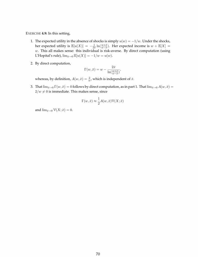
EXERCISE 4.9: In this setting,

1. The expected utility in the absence of shocks is simply u(w) = −1/w. Under the shocks,her expected utility is E[u(X)] = − 1

2x ln(w+xw−x). Her expected income is w + E[X] =

w. This all makes sense: this individual is risk-averse. By direct computation (usingL’Hopital’s rule), limx→0 E[u(X)] = −1/w = u(w).

2. By direct computation,

Γ(w, x) = w − 2xln(w+x

w−x),

whereas, by definition, A(w, x) = 2w , which is independent of x.

3. That limx→0 Γ(w, x) = 0 follows by direct computation, as in part 1. That limx→0A(w, x) =2/w 6= 0 is immediate. This makes sense, since

Γ(w, x) ≈ 12A(w, x)V(X; x)

and limx→0 V(X; x) = 0.

70

Documents

Carvajal Microeconomic Theory