Embed Size (px)
Citation preview
Department of Civil and Environmental Engineering
Stanford University
Report No.

The John A. Blume Earthquake Engineering Center was established to promote research and education in earthquake engineering. Through its activities our understanding of earthquakes and their effects on mankind’s facilities and structures is improving. The Center conducts research, provides instruction, publishes reports and articles, conducts seminar and conferences, and provides financial support for students. The Center is named for Dr. John A. Blume, a well-known consulting engineer and Stanford alumnus. Address: The John A. Blume Earthquake Engineering Center Department of Civil and Environmental Engineering Stanford University Stanford CA 94305-4020 (650) 723-4150 (650) 725-9755 (fax) [email protected] http://blume.stanford.edu
©2007 The John A. Blume Earthquake Engineering Center

ii
THIS PAGE LEFT BLANK
iv
ABSTRACT
ABSTRACT
The main objective of this research is to investigate the collapse performance of steel-framed
buildings under fires and to contribute to the development of methods and tools for
performance-based structural fire engineering. This research approach employs detailed
finite element simulations to assess the strength of individual members (beams and columns)
and indeterminate structural sub-assemblies (beams, columns, connections and floor
diaphragms). One specific focus of the investigation is to assess the accuracy of beam and
column strength design equations of the American Institute of Steel Construction (AISC)
Specification for Structural Steel Buildings. The simulation results show these design
equations to be up to 60 % unconservative for columns and 80-100 % unconservative for
laterally unbraced beams. Alternative equations are proposed that more accurately capture
the effects of strength and stiffness degradation at elevated temperatures. About eight
hundred simulations are performed to verify the proposed equations, accompanied by studies
on members with different steel strengths and section sizes.
The assessment technique for individual members is then extended to examine fire
effects for indeterminate gravity frame systems, including forces induced by restraint to
thermal expansion and nonlinear force redistribution due to yielding and large deformations.
Structural sub-assemblies are devised to examine indeterminate effects of gravity-framing in
a 10-story building, which is representative of design and detailing practice in the United
States. Three types of sub-assemblies are considered, including an interior gravity column, a
composite floor beam, and an exterior column-beam assembly. The sub-assembly models
include the restraining effects of floor framing that surrounds (both horizontally and
vertically) the localized compartment fire. The sub-assembly simulations support the
following observations and conclusions: (1) the rotational end restraint provided by the
columns above and below the fire story have a significant stabilizing effect on gravity
columns in the fire zone (providing up to a 40 % increase in strength above the pin-ended
condition at 400 °C), (2) vertical restraint of the heated column, by floor framing above the
fire story, does not significantly impact the strength limit state of the columns in the fire zone
(3) short of designing the building system with special redundant load paths, thermal

ABSTRACT
v
insulation is essential to avoid progressive collapse of highly-stressed gravity columns during
building fires (4) thermal insulation requirements for beams can be reduced while preserving
collapse resistance through enhanced connection details that are insulated, employ slotted
holes to permit thermal elongation, and incorporate thermally protected reinforcing bars in
the slab. These studies and conclusions are limited to evaluation of collapse safety and do
not address aspects related to post-fire repairs and loss assessment.
Uncertainty in the collapse behavior under fires is evaluated considering variability in
the gravity loading and structural response parameters. Using the statistical information to
quantify the random variables, the collapse probability of the column, beam and beam-
column sub-assemblies is assessed by the mean-value first-order second-moment (FOSM)
method. The collapse probability is conditioned with respect to the scaled intensity of fire
compartment gas temperature, which is treated as independent variable. These studies
indicate that the variability in the high-temperature steel yield strength is the most significant
factor in the uncertainty assessment. The studies further show that for the design fire
temperature, the probability of column failure ranges from 4 % to 38 % (β = 0.3-1.8) for
designs based on the AISC strength provisions (with φ = 0.9). These probabilities reduce to
0.5 % to 3 % (β = 1.9-2.6) based on the proposed equations (with φ = 0.9).

vi
ACKNOWLEDGEMENTS
S
This work was funded by the Fulbright graduate student fellowship and the John A. Blume
Earthquake Engineering Center.
This report was originally published as the Ph.D. dissertation of the first author.
The authors would like to thank Professors Sarah Billington, Helmut Krawinkler, Jack
Baker and Eduardo Miranda, for their advice on this research.
The authors gratefully acknowledge Dr. Liang Yu and Professor Karl H. Frank at the
University of Texas at Austin provided the essential test data of high strength bolts under
elevated temperatures. Professor Emeritus Brady R. Williamson provided priceless
research papers and reports. Dr. Barbara Lane and Dr. Susan Lamont helped the heat transfer
simulation with their expertise. Scott Hamilton worked on risk assessment and framework
of structural fire engineering with Professor Deierlein. Professor Paulo Vila Real at
University of Aveiro in Portugal kindly provided the most recent draft of Eurocode.
Professor Richard Liew at the National University of Singapore also provided his
research papers and proceedings of past fire workshops. Dr. Ryoichi Kanno at Nippon
Steel kindly arranged the use of the test data of steel at elevated temperatures performed
by the Japan Iron and Steel Federation. Corus (British Steel) Swinden Laboratories
provided their test data on steel beams at elevated temperatures. Karen Greig, Head
Librarian at Engineering Library at Stanford University, obtained papers regarding
structural fire engineering.

vii
TABLE OF CONTENTS
Chapter 1 Introduction 1
1.1 Overview 1
1.1.1 Background and Focus of This Research 1
1.1.2 Performance-Based Fire Engineering 2
1.1.3 Role of Structural Fire Engineering 3
1.1.4 Behavior of Steel Structures Exposed to Fire 4
1.1.5 Domains for Limit-state Evaluation 5
1.1.6 Disaster of the World Trade Center 6
1.1.7 Uncertainties in Structural Fire Engineering 6
1.2 Objectives 7
1.3 Scope 8
1.4 Organization 9
Chapter 2 Overview of Steel Structures Exposed to Fire 11
2.1 Past Fire Disasters 11
2.1.1 Fires on Steel Structures 11
2.1.2 Broadgate Phase 8 13
2.1.3 One Meridian Plaza 15
2.1.4 World Trade Center Building 7 16
2.1.5 Windsor Building 20
2.1.6 Cardington Fire Test 23
2.1.7 Summary of Past Fire Disaster Review 25
2.2 Mechanical Properties of Steel under Elevated Temperatures 25
2.2.1 Experimental Results 25
2.2.1.1 Experiments by Harmathy and Stanzak 26
2.2.1.2 Experiment by Skinner 28
2.2.1.3 Experiments by DeFalco 29
2.2.1.4 Experiments by Fujimoto et al. 32
2.2.1.5 Experiments by Kirby and Preston 33
TABLE OF CONTENTS
viii
2.2.1.6 Comparison of the Experiments 35
2.2.2 Equations of Stress-strain Curves 38
2.2.2.1 Eurocode Stress-strain Curves 38
2.2.2.2 AS4100 Stress-strain Curves 40
2.2.2.3 AIJ Stress-strain Curves 41
2.2.2.4 AISC Stress-strain Curves 44
2.2.2.5 Comparison of the Equations of Stress-strain Curves 45
2.2.3 Experiments by JISF 49
Chapter 3 Analysis of Individual Members 51
3.1 Summary 51
3.2 Introduction 51
3.3 Basis of Member Strength Evaluations 53
3.3.1 Steel Properties under Elevated Temperatures 55
3.4 Finite Element Simulation Model 57
3.5 Column Strength Assessment 61
3.5.1 AISC Column Strength Equations 62
3.5.2 EC3 Column Strength Equations 62
3.5.3 Assessment of Column Strengths 64
3.5.4 Proposed Column Strength Equations 67
3.5.5 Column Test Data 68
3.5.6 Influence of Yield Strength and Section Geometry 69
3.6 Beam Strength Assessment 70
3.6.1 AISC Beam Strength Equations 70
3.6.2 EC3 Beam Strength Equations 72
3.6.3 Proposed Beam Strength Equations 73
3.6.4 Assessment of Beam Strengths 74
3.7 Beam-Column Strength Assessment 78
3.7.1 AISC Beam-Column Strength Equations 79
3.7.2 Proposed Beam-Column Strength Equations 80
3.7.3 EC3 Beam-Column Strength Equations 80
3.7.4 Assessment of Beam-Column Strengths 80
3.8 Summary and Conclusions 83

TABLE OF CONTENTS
ix
3.9 Limitations and Future Research 84
Chapter 4 Analysis of Gravity Frames 87
4.1 General 87
4.1.1 Overview 87
4.1.2 Benchmark Office-type Building Design 88
4.1.3 Failure Mechanisms and Sub-assembly Analysis Models 90
4.1.4 Time-temperature Relationships in Localized Fire 92
4.1.5 Organization of Chapter 4 93
4.2 Evaluation of Interior Column Sub-assembly 93
4.2.1 Summary 93
4.2.2 Introduction 93
4.2.3 Analysis Model 96
4.2.3.1 Modeling of System 96
4.2.3.2 Modeling of Column 98
4.2.3.3 Modeling of Constraint Springs 101
4.2.4 Evaluation of Critical Temperatures 106
4.2.5 Comparison between Design Equations and Sub-assembly Simulations 111
4.2.6 Improvement of Structural Robustness 112
4.2.7 Conclusions 114
4.3 Evaluation of Beam Sub-assembly 115
4.3.1 Summary 115
4.3.2 Introduction 115
4.3.3 Analysis Model 116
4.3.3.1 Modeling of System 116
4.3.3.2 Modeling of Steel Beam 117
4.3.3.3 Modeling of Concrete Slab 118
4.3.3.4 Modeling of Bolted Connection 119
4.3.3.5 Modeling of Longitudinal Constraint by Floor Framing 126
4.3.4 Evaluation of Behavior and Limit-state 128
4.3.4.1 Performance of Typical Design 128
4.3.4.2 Performance of Alternative Design 130
4.3.4.3 Effect of Longitudinal Constraint 133

TABLE OF CONTENTS
x
4.3.5 Conclusions 134
4.4 Evaluation of Exterior Column Sub-assembly 135
4.4.1 Overview 135
4.4.2 Analysis Model 136
4.4.2.1 Modeling of System 136
4.4.2.2 Modeling of Bolted Connection 139
4.4.3 Evaluation of Behavior and Limit-state 142
4.4.3.1 Basis of Simulations 142
4.4.3.2 Simulation Results 142
4.4.3.3 Alternative Connection Design 144
4.4.4 Conclusions 145
4.5 Overall Limit-state Evaluation 146
4.6 Conclusions of Gravity Frame Analysis 147
Chapter 5 Probabilistic Assessment 149
5.1 Overview 149
5.2 Structural Uncertainties in Fire Engineering 149
5.2.1 Summary of Statistical Data 149
5.2.2 Variability of Yield Strength of Steel 151
5.2.3 Variability of Longitudinal Spring Stiffness for Interior Column 153
5.2.4 Variability of Shear Strength of Bolts 156
5.2.5 Variability of Longitudinal Strength of Springs for Bolted Connections 160
5.2.6 Variability of Deformation Capacity of Bolted Connections 160
5.2.7 Variability of Time-temperature Relationships in Compartment Fire 162
5.3 Probabilistic Studies 165
5.3.1 Sensitivity of Critical Temperatures to Uncertainties 165
5.3.1.1 Sensitivities in Interior Column Sub-assembly Study 166
5.3.1.2 Sensitivities in Beam Sub-assembly Study 167
5.3.1.3 Sensitivities in Exterior Column Sub-assembly Study 168
5.3.2 Collapse Probabilities of Sub-assemblies given Temperatures 170
5.3.3 Reliability of AISC-LRFD Fire Equation 172
5.3.4 Conclusions 178

TABLE OF CONTENTS
xi
Chapter 6 Conclusions 181
6.1 General 181
6.2 Summary 182
6.2.1 Steel Properties at Elevated Temperatures 182
6.2.2 Past Fire Disasters 183
6.2.3 Member-based Strength Study 183
6.2.4 Benchmark Building Study 184
6.2.5 Probabilistic Studies 184
6.3 Major Findings and Conclusions 185
6.3.1 AISC Member-based Design Criteria 185
6.3.2 Effect of Residual Stress and Local Buckling 185
6.3.3 Proposed Design Criteria for AISC 186
6.3.4 Steel-framed Building under Localized Fire 186
6.3.5 Longitudinal Constraint of Interior Column 187
6.3.6 Longitudinal Constraint of Beam 188
6.3.7 Properties of Bolted Connections 188
6.3.8 Evaluation of Structural Uncertainties 189
6.3.9 Probabilistic Studies 189
6.4 Design and Analytical Modeling Recommendations 190
6.4.1 Design Recommendations 190
6.4.2 Analytical Modeling Recommendations 191
6.5 Future Work 192
6.5.1 Member-based Strength Evaluation 192
6.5.2 Performance Evaluation of Steel Buildings under Fires 192
Appendix A Supplemental Studies on Individual Members 195
A.1 Tangent Modulus Theory 195
A.1.1 Flexural Buckling 195
A.1.2 Lateral Torsional Buckling 200
A.2 Modeling Comparison of Individual Members 204
A.2.1 Fiber Model 204
A.2.2 Effect of Local Buckling 205
A.2.3 Post Buckling Strength 206

TABLE OF CONTENTS
xii
A.3 Effect of Uncertain Conditions 209
A.3.1 Overview 209
A.3.2 Non-uniform Temperature Distribution 209
A.3.3 Imperfections 212
A.3.4 Boundary Conditions 213
A.3.5 Steel Properties 216
A.4 Other Miscellaneous Studies 218
A.4.1 Temperature Distribution of Composite Beams 218
A.4.2 Modeling Comparison of Composite Beam 220
A.4.3 Effect of Heat Conduction 222
Appendix B Reference Equations 225
B.1 Conversion of Units 225
B.2 Symbols 226
B.3 Design Equations of Steel at Elevated Temperatures 228
B.3.1 Eurocode 3 228
B.3.2 AS4100 231
B.4 Time-temperature Relationships 231
B.4.1 Parametric Fire Curve 231
B.4.2 Step-by-step Steel Temperature Simulation 236
B.5 FOSM 238
Appendix C JISF Experiment 241
C.1 Summary 241
C.2 Data Conditions 241
C.3 General 241
C.4 JISF Stress-strain Curves 242
C.5 Comparison of the Test Data with AIJ and EC3 250
C.6 Statistical Study 254
Bibliography 259
Symbols 267

xiii
LIST OF TABLES
Chapter 2 Overview of Steel Structures Exposed to Fire
Table 2-1 Past major fire disasters of steel buildings 12
Table 2-2 Chemical composition of steels by Harmathy and Stanzak (Wt%) 26
Table 2-3 Chemical composition of steel by Skinner (Wt%) 28
Table 2-4 Chemical composition of steel by DeFalco (Wt%) 32
Table 2-5 Chemical composition of steel by Fujimoto et al. (Wt%) 32
Table 2-6 Chemical composition of steel by Kirby and Preston (Wt%) 34
Table 2-7 Comparison of steel experiments at elevated temperatures 36
Table 2-8 Coefficients in AIJ equations for stress-strain curves 43
Chapter 3 Analysis of Individual Members
Table 3-1 Stress-strain reduction factors in EC3 57
Table 3-2 Steel section data 64
Table 3-3 Measured and calculated strengths of column tests 68
Chapter 4 Analysis of Gravity Frames
Table 4-1 Section sizes (mm) 90
Table 4-2 Section sizes of columns in 5- and 20-story buildings (mm) 110
Table 4-3 Critical temperatures with different number of building stories 110
Table 4-4 Values of reduction factor of bolt strength 124
Table 4-5 Comparison of the critical temperatures 132
Table 4-6 Effect of the constraint stiffness to the critical temperatures 134
Table 4-7 Limit-states for exterior column sub-assembly model 144
Table 4-8 Critical time, steel temperatures and failure mechanisms of sub-assemblies 146
Chapter 5 Probabilistic Assessment
Table 5-1 Statistical data for uncertainties 150
Table 5-2 Symbols regarding statistical properties of steel strength 152
Table 5-3 Ratios of upper and lower bounds of factors for the vertical spring 155

LIST OF TABLES
xiv
Table 5-4 Combinations of factors for vertical spring of interior column 156
Table 5-5 Mean and c.o.v. of shear strength of bolts 160
Table 5-6 Band of influential factors for fire simulation 163
Table 5-7 Maximum temperatures in variation of fire simulation (°C) 165
Table 5-8 Critical temperature with various constraint stiffness 168
Table 5-9 Variability of the collapse probability with respect to gas temperature 172
Table 5-10 Comparison of expected, nominal, and factored load (N/m2) 173
Appendix A Supplemental Studies on Individual Members
Table A 1 Combinations of non-uniform temperature distributions 210
Table A 2 Section sizes of beam tested by Wainman and Kirby (mm) 219
Table A 3 Thermal properties of steel column 223
Appendix B Reference Equations
Table B-1 Conversion of temperature units 225
Table B-2 Conversion of length and force units 225
Table B-3 Conversion of pressure units 226
Table B-4 Symbols in AISC and Eurocode 226
Table B-5 Parameters and conditions for parametric fire curves 234
Table B-6 Thermal properties of steel and fire insulation 237
Appendix C JISF Experiment
Table C-1 Number of tests for each steel type and temperatures 243
Table C-2 Elastic modulus and yield strength (Gr.50) defined in AIJ, EC3, and AISC 250
Table C-3 Mean and coefficient of variation of 1 % and 2 % strength 256

xv
LIST OF FIGURES
Chapter 1 Introduction
Figure 1-1 Assessment strategy 8
Chapter 2 Overview of Steel Structures Exposed to Fire
Figure 2-1 Photos of Broadgate fire 14
Figure 2-2 Photos of One Meridian Plaza fire 16
Figure 2-3 Floor plan and damages of WTC 7 17
Figure 2-4 Fires observed from the east and north face of WTC 7 18
Figure 2-5 Probable global collapse mechanism of WTC 7 19
Figure 2-6 Exterior view of Windsor Building before and after the fire 21
Figure 2-7 Detailed photos of Windsor Building fire 22
Figure 2-8 Photos of the Cardington Fire Test 24
Figure 2-9 Floor framing and test locations 24
Figure 2-10 Stress-strain curves by Harmathy and Stanzak (1970) 27
Figure 2-11 Stress-strain curves by Skinner (1972) 29
Figure 2-12 Stress-strain curves by DeFalco (1974) 31
Figure 2-13 Stress-strain curves by Fujimoto et al. (1980, 81) 33
Figure 2-14 Stress-strain curves by Kirby and Preston 35
Figure 2-15 Comparison of stress-strain curves in experiments 37
Figure 2-16 Stress-strain curves defined by EC3 39
Figure 2-17 Stress-strain curves defined by AS4100 41
Figure 2-18 Stress-strain curves defined by AIJ 42
Figure 2-19 Reduction ratios in the stress-strain curves defined by AIJ 44
Figure 2-20 Stress-strain curves defined by AISC 45
Figure 2-21 Comparison of stress-strain curves (equations and experiments) 47
Figure 2-22 Eurocode stress-strain curve (500 °C) with hardening at large strains 48
Figure 2-23 Comparison of normalized stress-strain curves (equations and experiments) 49
Figure 2-24 Comparison of stress-strain curves by JISF, EC3, and AIJ 50

LIST OF FIGURES
xvi
Chapter 3 Analysis of Individual Members
Figure 3-1 Comparison of temperature and load control analyses 54
Figure 3-2 Stress-strain response at high temperatures as defined by EC3 56
Figure 3-3 Shell finite element mesh and boundary conditions 59
Figure 3-4 Load versus displacement response from FEM simulations under ambient and elevated temperatures 59
Figure 3-5 Influence of residual stresses (W14×90 Gr. 50 column at 500 °C) 60
Figure 3-6 Critical compressive strengths of W14×90 Gr.50 column 66
Figure 3-7 Percentage error in the calculated compression strength of W14×90 Gr.50 column at 500 °C 67
Figure 3-8 Comparative assessment of column compression strength at 500 °C 69
Figure 3-9 Critical bending moment strengths of W14×22 Gr.50 beam 76
Figure 3-10 Percentage error in the calculated bending moment strength of W14×22 Gr.50 beam at 500 °C 76
Figure 3-11 Comparative assessment of beam bending moment strength at 500 °C 77
Figure 3-12 Critical axial load and moment strengths of W14×90 Gr.50 (λ=60) beam-column 82
Figure 3-13 Comparative assessment of beam-column strengths at 500 °C 83
Chapter 4 Analysis of Gravity Frames
Figure 4-1 Floor plan of benchmark building design 88
Figure 4-2 Details of column-beam shear tab connections 89
Figure 4-3 Possible failure mechanisms (column line 3) 91
Figure 4-4 Sub-assembly analysis models 91
Figure 4-5 Time-temperature relationships in a fire simulation 92
Figure 4-6 Analysis model of a column with constraint springs 95
Figure 4-7 Analysis model for column buckling collapse mechanism 97
Figure 4-8 Preliminary model for interior column 99
Figure 4-9 Axial load carrying capacity of the interior column at elevated temperatures 99
Figure 4-10 Comparison of column strength with different models 100
Figure 4-11 Post buckling deformation of shell element model 101
Figure 4-12 Analysis model of beams for vertical spring stiffness of floor structure 102
Figure 4-13 Rotational properties of shear-tab connections 103
Figure 4-14 Analysis model of floor structure for in-plane stiffness calculation 104

LIST OF FIGURES
xvii
Figure 4-15 Longitudinal constraint stiffness of beams 105
Figure 4-16 Vertical resistance of floor structure 106
Figure 4-17 Resistance of the system under elevated temperatures 108
Figure 4-18 Vertical displacement of the interior column under elevated temperatures 109
Figure 4-19 Critical axial strength of W14×90 (4 m) based on member-based and sub-assembly approaches 111
Figure 4-20 Options for strengthened connections 112
Figure 4-21 Total vertical load carrying capacity with strengthened connection for Beam a and b 113
Figure 4-22 Vertical displacement of the buckled column with improved beam connection 113
Figure 4-23 System of finite element composite beam model in floor framing 117
Figure 4-24 Temperature distribution of composite section 118
Figure 4-25 Compressive stress-strain curve of concrete 119
Figure 4-26 Gravity load supporting systems of beams at elevated temperatures 119
Figure 4-27 Detail of beam connection 120
Figure 4-28 Single shear bolt test by Yu (2006) 120
Figure 4-29 Load-displacement relationships of single shear connections by Yu (2006) 121
Figure 4-30 Maximum single shear strength of A325 bolts by Yu (2006) 122
Figure 4-31 Force-displacement relationship model of bolted connection 123
Figure 4-32 Reduction factor of bolt strength by ECCS 124
Figure 4-33 Comparison of force-displacement relationships of bolted connection between analysis model and test data by Yu (2006) 126
Figure 4-34 Analysis model for constraint stiffness 127
Figure 4-35 Mid-span displacement and modeling comparison 128
Figure 4-36 Post peak-strength evaluation of bolted connection 129
Figure 4-37 Proposed design options for bolted connections 130
Figure 4-38 Performance of composite beams with alternative design options for the connections 131
Figure 4-39 Alternative connection detail of secondary beams to prevent shear failure at elevated temperatures 132
Figure 4-40 Influence of the longitudinal constraint stiffness 133
Figure 4-41 Failure mechanisms simulated with exterior column sub-assembly 136
Figure 4-42 System of exterior column sub-assembly model 138

LIST OF FIGURES
xviii
Figure 4-43 Lateral constraint by floor slab with membrane action 138
Figure 4-44 Comparison of compartment fire for exterior column sub-assembly simulations 139
Figure 4-45 Detail of exterior column connection 140
Figure 4-46 Comparison between analysis model and test data by Yu (2006) of longitudinal force-displacement relationships of beam-column bolted connection 141
Figure 4-47 Time-temperature relationships in a fire simulation 142
Figure 4-48 Displacement for the exterior column sub-assembly model 143
Figure 4-49 Connection details between external column and beam 145
Chapter 5 Probabilistic Assessment
Figure 5-1 Variation of tested steel strength under elevated temperatures 153
Figure 5-2 Variation of vertical spring properties 156
Figure 5-3 Shear strength of bolts at elevated temperatures 157
Figure 5-4 Shear strength of bolts normalized with ECCS strength 159
Figure 5-5 Uncertainty of deformation capacity of bolted connection 162
Figure 5-6 Variations of time-temperature relationships 164
Figure 5-7 Sensitivity of the critical temperature of interior column sub-assembly 166
Figure 5-8 Sensitivity of the critical temperature of beam sub-assembly 167
Figure 5-9 Sensitivity of the critical beam temperature of exterior column sub-assembly 169
Figure 5-10 Time-temperature relationships in a fire simulation 171
Figure 5-11 Collapse probability of sub-assemblies 171
Figure 5-12 Load and resistance relationships in AISC-LRFD 173
Figure 5-13 Probability of failure of W14×90 column at 500 °C with varied length 175
Figure 5-14 φ factors for 0.47 % (β = 2.6) probability of failure of W14×90 column at 500 °C with varied length 175
Figure 5-15 Probability of failure of W14×90 (L = 4 m) column with varied temperatures 176
Figure 5-16 φ factors for 0.47 % (β= 2.6) probability of failure of W14×90 (L = 4 m) column with varied temperatures 177

LIST OF FIGURES
xix
Appendix A Supplemental Studies on Individual Members
Figure A-1 Strain level and residual stress 197
Figure A-2 Critical strength of columns by tangent modulus theory 198
Figure A-3 Stress-strain curves with the average tangent stiffness in section 199
Figure A-4 The critical strength of W14×90 column 200
Figure A-5 Lumped fiber model 201
Figure A-6 Critical moment by tangent modulus theory 203
Figure A-7 Comparison of the critical moment by analyses and tangent modulus theory 204
Figure A-8 Integration points in fiber model section 205
Figure A-9 Effect of imperfection for local buckling 206
Figure A-10 Post buckling strength (W14×90, Gr.50, L=4m) 207
Figure A-11 Post-buckling behavior for LTB 208
Figure A-12 Non-uniform temperature distribution modes 210
Figure A-13 Sensitivity of critical strength to non-uniform temperature distribution 211
Figure A-14 Sensitivity of critical strength to non-uniform temperature distribution for the weak axis 212
Figure A-15 Sensitivity of critical strength to imperfections 213
Figure A-16 Sensitivity of critical strength to boundary conditions at 500 °C 215
Figure A-17 Sensitivity of critical strength to boundary conditions at 20 °C 216
Figure A-18 Sensitivity of critical strength to steel properties at 500 °C 217
Figure A-19 Sensitivity of critical strength to steel properties at 20 °C 218
Figure A-20 Temperature distribution of composite section 218
Figure A-21 Beam experiment by Wainman and Kirby (1988) 219
Figure A-22 Recorded temperatures in three sections by Wainman and Kirby (1988) 220
Figure A-23 Comparison between analysis and test by Wainman and Kirby (1988) 221
Figure A-24 Study model for heat conduction 222
Figure A-25 Temperature increase by heat conduction 224
Appendix B Reference Equations
Figure B-1 Section axes in AISC and Eurocode 226

LIST OF FIGURES
xx
Appendix C JISF Experiment
Figure C-1 JISF stress-strain curves (SM490A Plate) 244
Figure C-2 JISF stress-strain curves (SM490A Wide Flange) 245
Figure C-3 JISF stress-strain curves (SM490AW Plate) 246
Figure C-4 JISF stress-strain curves (SN490C Plate) 247
Figure C-5 JISF stress-strain curves (STKN400B) 248
Figure C-6 JISF stress-strain curves (STKN490B) 249
Figure C-7 Comparison of stress-strain curves (up to 2.5 % strain) 252
Figure C-8 Comparison of stress-strain curves (up to 10 % strain) 253
Figure C-9 Comparison of stresses at 1 % strain 255
Figure C-10 Comparison of stresses at 2 % strain 255
Figure C-11 JISF paper (page 1) 257
Figure C-12 JISF paper (page 2) 258

1
CHAPTER 1 INTRODUCTION
1 INTRODUCTION
1.1 OVERVIEW
1.1.1 Background and Focus of This Research
Traditional building-code design provisions for fire resistance in steel-framed buildings are
highly prescriptive and empirically based. As a result, structural engineers have both limited
means and opportunities to devise, assess and implement alternative solutions for fire
resistance that may be more cost-effective than conventional solutions. So-called
performance-based approaches seek to change this by offering more transparent and
scientifically-based methods to assess impact of fires on buildings. Performance-based fire
engineering and design encompasses a broad range of expertise and considerations, which
span far beyond the discipline of structural engineering. Performance-based fire engineering
and design has received considerable attention in recent years, as evidenced by major
specialty conferences (e.g., SFPE 2004), books (e.g., SFPE 2007, Custer and Meacham 1997)
and many published papers. For example, in related research at Stanford University,
Hamilton and Deierlein (2004) have explored the parallels between performance-based
approaches for structural design to resist fire and earthquakes.
This research is intended to contribute to one aspect of performance-based structural fire
engineering involving the development of models and criteria to assess the collapse
performance of steel-framed structures at elevated temperatures. The specific focus is on
evaluating the strength limit state of gravity framing systems, which are likely to be the most
vulnerable components of steel-framed buildings subjected to fire. The research employs the
development, calibration and application of detailed nonlinear analyses to investigate the
strength limit states of individual steel members and sub-assemblies of members subjected to
combined gravity loads and elevated temperatures. In addition to assessing the response of

CHAPTER 1. INTRODUCTION
2
conventional steel building details, this research also examines alternative structural design
and details to improve collapse safety.
1.1.2 Performance-Based Fire Engineering
In the progression from prescriptive design toward performance-based design, structural
engineers are taking more responsibility for assessing structural performance and relating its
implications to key stakeholders, including building owners, building code-officials, and
society at large. Performance-based approaches allow more flexibility in the structural
design, since they relieve engineers of the mandate to follow prescriptive design
requirements. Specifically, performance-based approaches may relieve the prescriptive
design provisions that require specific thermal insulation on steel members to limit steel
temperatures during fires. Past experience shows that this fire insulation works well;
however, the prescribed insulation requirements usually do not distinguish between
alternative fire exposures and differences in structural behavior for different buildings. For
example, the standard fire curve, which is the time-temperature relationship commonly used
for evaluating the fire resistance of materials, does not represent actual flashover fire
characteristics in steel-framed buildings. Rather, it is intended for qualification testing of
structural components and insulating materials, where the limit state criteria does not
necessarily relate to real behavior in buildings. While such approaches were a practical
necessity when computer analysis technology was less developed and structural simulation
under fire conditions was difficult, the over-reliance on empirical testing using the standard
fire curve has become an obstacle to more thoughtful and case-specific design.
In contrast, a more rational and scaleable framework for design should enable the use of
simulation methods to assess structural response to fire, including evaluation of the inherent
uncertainties in the fire and its effects on the structure (e.g., Hamilton and Deierlein 2004).
Such an approach in structural fire engineering (or performance-based fire engineering,
PBFE) makes it possible to develop a fire-resistant structural design by explicitly evaluating
the behavior of the buildings under fires. This approach is especially useful for buildings that
are not addressed well by prescriptive approaches, such as high-rise buildings or buildings
with unique functions and/or configurations. For such buildings, PBFE can enable one to
simulate explicitly the structural behavior under fires, and then determine the required
thermal insulation (or other protective measures) to ensure that the building has the desired
level of performance. It is reported that conventional fire insulation can add up to 30 % to

CHAPTER 1. INTRODUCTION
3
the construction cost for steel building frames (Lawson, 2001). Thus, there is a potentially
significant economic motivation to design buildings using PBFE rather than common
prescriptive requirements. Depending on the design philosophy and goals, financial benefit-
cost analyses may show that it is more cost-effective to allow certain levels of structural
damage in extreme and rare fires. Alternatively, more stringent requirements may be
appropriate to further reduce the risk of structural collapse where it has significant
implications on life safety. In order to use such a design philosophy, methods and criteria are
needed to simulate realistically structural behavior under fires.
1.1.3 Role of Structural Fire Engineering
Overall, fire protection engineering involves many engineering fields such as materials,
mechanical equipment, chemistry, human behavior, heat transfer, statistics, and structures.
Each field has its unique relevance to fire safety, including efficient measures to control both
the risk of fire ignition/growth and possible resulting impacts of fire. Approaches to control
fire damage are generally categorized as either active or passive measures. Mechanical or
human interventions are active measures, such as sprinklers, fire alarms, or detection
systems. Passive measures are incorporated with built-in systems such as fire insulation on
structural members or fire-rated room partitions, which create fire compartments that inhibit
fire spread. Active measures are especially important for controlling the early stages of the
fire, limiting fire growth, and reporting the fire to fighting personnel. Passive measures are
important in the case that these active measures fail and the fire fully develops into a so
called “flashover fire”. Passive measures are the main focus of structural fire engineering,
though the performance requirements for passive systems may depend on active systems in
the buildings.
Simulations required to evaluate structural behavior under fires include (1) simulation of
fire behavior, (2) simulation of heat transfer to the structure, and (3) simulation of structural
behavior. The primary focus of structural fire engineering is to assess structural behavior.
Structural temperatures can be simulated in some advanced analyses; however, simulation of
the fire behavior itself is generally outside the scope of structural engineering. Interactions
between these simulations are relatively limited and it is generally assumed that each
component of the analysis (fire, thermal, and structural) can be performed independently.
This is advantageous as it allows for structural behavior under fire to be simulated based on
either peak temperature or time-temperature relationships in the structural members. Steel

CHAPTER 1. INTRODUCTION
4
temperatures (either peak values or time-varying values) and be related to parametric fire
curves using straightforward heat transfer analyses.
While structural simulation is only a part of the overall process necessary to evaluate
building safety against fire, research on structural behavior is important because structural
collapse is potentially devastating. Depending on the circumstances, human, economic, and
physical loss caused by a structural collapse can overwhelm the damage caused by the initial
fire.
1.1.4 Behavior of Steel Structures Exposed to Fire
One of the ultimate goals of structural fire engineering is to simulate behavior and limit state
under fires. As discussed further in the next section, the risks and safety of the structures
under fires can be evaluated in terms of the alternative metrics of strength (load resistance),
temperature or time. Whichever metric is used, the primary behavioral effect in structural
assessment is the degradation in stiffness and strength of structural materials at high
temperatures and the potential for localized structural failure to trigger global collapse.
Thermal expansion is also a significant issue in structural fire engineering, in addition to
the material deterioration at elevated temperatures. Effects of thermal expansion vary
depending on the longitudinal constraint of heated members. Under elevated temperatures,
longitudinal elongation is induced when the constraint is relatively low; while compressive
axial force is induced when the constraint is high. There has been some debate whether or
not thermal expansion is critical at the structural limit state, because thermally induced force
tends to eventually decrease at this limit state with the deteriorated material under the
elevated temperatures. These discussions are inconclusive and further study is needed.
Three-dimensional (3D) effects are more significant for structural behavior under fires,
as compared to other types of extreme loadings such as wind and earthquakes. This is
because initially localized structural damage in fires spreads three dimensionally to the
connecting members.
Cast-in-place concrete slabs and composite beam slab systems are typically used in steel
buildings. It is known that this composite effect significantly enhances performance of steel
frames under fire conditions. Temperatures of the concrete slab under fire conditions are
generally lower than steel members and the strength degradation of reinforced concrete is
much less. Furthermore, concrete slab systems potentially have high load carrying capacity
under large deformation, due to catenary action. However, evaluating this enhanced

CHAPTER 1. INTRODUCTION
5
performance is difficult, because of the complexity of how the composite system behaves
under large deformations. Specifically, simulating the behavior of shear stud connections
and the interaction between concrete slabs and steel beams is difficult and further research is
needed.
The behavior of bolted and welded connections between members is also influential to
overall frame behavior. Strength deterioration in connections is more severe than that of
steel members, making it possible for connection failure to be critical under fire conditions.
Also, large deformations of beams can induce significant tensile forces under catenary action,
and the strength of typical shear-tab connections may not be large enough to support these
forces.
1.1.5 Domains for Limit-state Evaluation
Evaluation of structural limit states under fire conditions can be performed in one of three
domains: time, temperature, and strength. Evaluation of the structural limit state in the time
domain is most closed associated with requirements for evacuation or fire fighting activities,
which are calculated as a function fire development and suppression times. In the
temperature domain, the collapse performance is evaluated in term of the critical
temperatures in the steel members. This domain has the advantage of enabling the structural
performance to be evaluated independent of fire growth behavior. Limit states calculated in
the time and temperature domains can be directly converted once the relationship between
the time and temperature during the fire is provided.
Critical strength (i.e. maximum applied load level that the structure can carry) is
calculated under a specified constant temperature in the strength domain. For a specified
maximum temperature, the critical strength is calculated and compared to the applied gravity
load assumed in the design. This approach is advantageous in terms of numerical analysis,
since loads and displacements are common control variables used in structural analysis
software. On the other hand, time and temperature can only be accounted for indirectly in
analysis or by using specialized analysis software. Structural performance can be evaluated
in either of these domains, and the domain should be properly selected to meet the purpose of
the analytical simulation and performance evaluation.

CHAPTER 1. INTRODUCTION
6
1.1.6 Disaster of the World Trade Center
Since the terrorism attack and collapse of the World Trade Center buildings on September
11th of 2001, in New York City, behavior of steel buildings exposed to fire has been a
popular topic of study and debate. Behavior of individual members and connections had
been the focus of much of the research before the disaster, and there are still many research
needs for element-based studies. However, the complete collapse of three major buildings
(WTC towers 1 and 2 and the 47 story WTC 7 building) highlighted the importance of
understanding the overall structural system performance.
It is generally accepted that redundancy is desirable in structures; and this is especially
true for structural fire design. This concept follows the “fail-safe” concept, which implies
that a loss in the load carrying capacity of some members will not lead to global building
collapse. Surrounding elements of the damaged structure should provide an alternative load
carrying path. Therefore, redundancy can be provided by statically indeterminate structures;
however, even highly indeterminate structures do not necessarily ensure the presence of
alternative load carrying paths that can resist progressive collapse. Past discussions
regarding redundancy have often remained abstract, and have rarely resulted in specific fire
design recommendations.
1.1.7 Uncertainties in Structural Fire Engineering
Fires are similar to earthquakes, being rare events with high consequence. This characteristic
makes uncertainty assessment a key subject of this research. There are many uncertain
factors including fire occurrence and behavior in the overall fire risk assessment. From the
structural fire engineering point of view, there are many uncertain aspects of the loads and
strengths. Load and Resistance Factor Design (LRFD) is designed to deal with uncertainties
and lead to a design with an acceptable probability of failure. The LRFD method for
structural fire engineering is still developing, in part because the acceptable level of
probability of failure under fires has not been explicitly defined. Development of fire hazard
analysis models is especially needed for this purpose in addition to the development of
structural analysis technology. Controlling the probability of failure is one of the most
important goals of performance-based design. Since some of the statistical information
regarding structural responses needed for uncertainty assessment is not readily available,

CHAPTER 1. INTRODUCTION
7
engineering assumptions or judgments are used in this research when appropriate to enable
probabilistic assessment of failure of steel buildings under fire conditions.
1.2 OBJECTIVES
The objectives of this research are summarized in following points:
(1) Synthesize and interpret current design specifications for structural fire engineering
for steel buildings, and contribute to developing structural fire design methodologies
based on performance-based design concepts.
(2) Advance knowledge to systematically evaluate fire-induced collapse performance of
steel framed buildings under fires.
(3) Investigate the member-based strength criteria at elevated temperatures defined in the
design specifications of American Institute of Steel Construction (AISC, 2005), and
assess the accuracy of these provisions relative to the assessment of strength limit-
states simulated with rigorous finite element analysis. Where appropriate, propose
improved member-based strength design criteria, whose accuracy is validated by
analytical simulations.
(4) Assess performance of gravity framing in an archetypical steel-framed building under
localized fire, and explore improved design concepts and details, including analytical
validation.
(5) Investigate variability and uncertainties in the important aspects in the structural
performance evaluations under fires. Probabilistically assess member-based strengths
and building performance. Use these findings to develop a basis for probabilistic risk
assessments in structural fire engineering.
Meeting these objectives requires integration of past research to draw practical implications
on design practice. Integration is necessary to cover various subjects of structural fire
engineering, including analysis of members and frames, and simulations from fire behavior to
structural failure. Knowledge from not only structural fire engineering, but also other fields
such as earthquake engineering, will be integrated. Regarding practical significance, the
directions of this research was selected to focus on topics that are expected to provide
findings and conclusions that will be of practical use in the engineering profession.
CHAPTER 1. INTRODUCTION
8
The significance of frame analysis in structural fire engineering is to evaluate
numerically possible alternative load carrying paths using rigorous analytical simulations.
Showing processes and results of frame analysis based on research of individual members
and details is greatly influential to practical structural fire design. In other words, this work
is to evaluate concretely and objectively structural reliability and redundancy. The ultimate
goal is to develop and apply rigorous analytical simulations to systematically evaluate the
collapse limit-state for buildings of various framing configurations and fire scenarios.
1.3 SCOPE
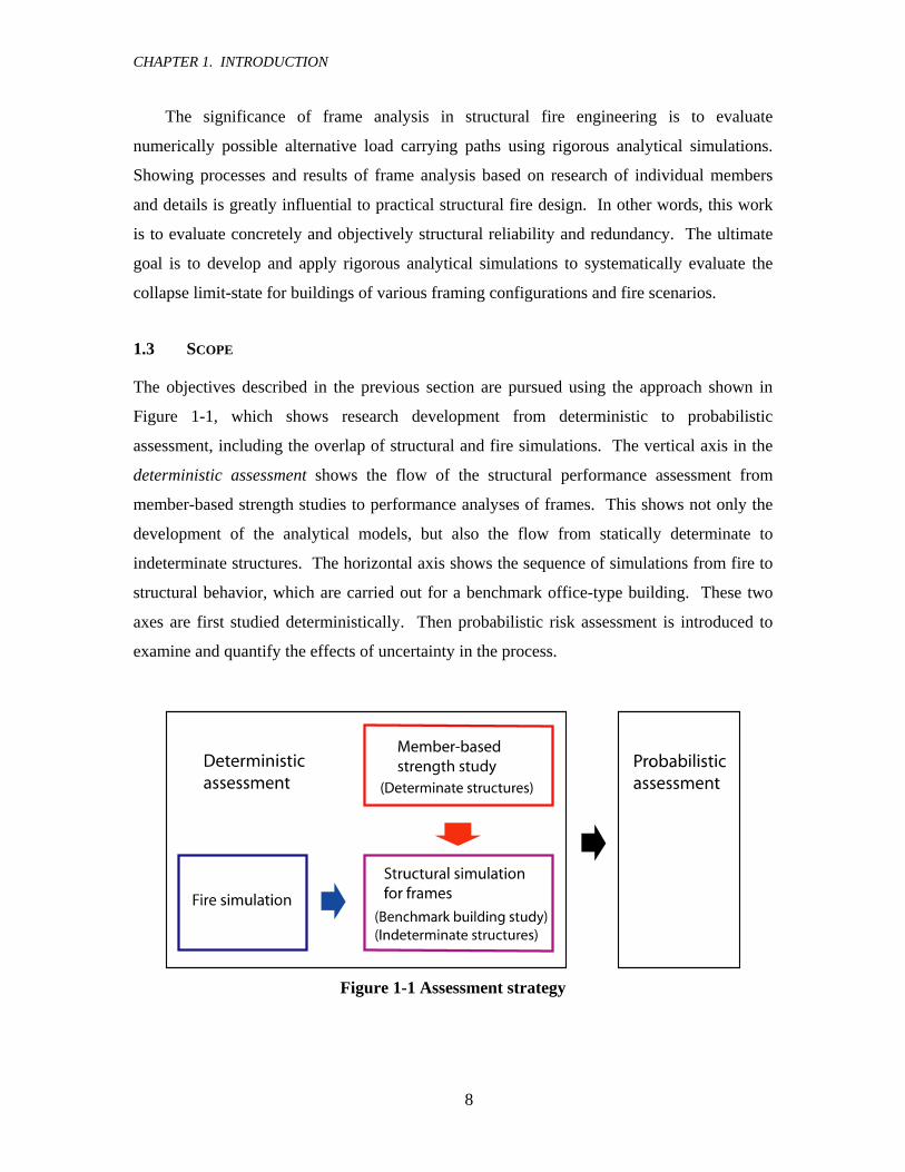
The objectives described in the previous section are pursued using the approach shown in
Figure 1-1, which shows research development from deterministic to probabilistic
assessment, including the overlap of structural and fire simulations. The vertical axis in the
deterministic assessment shows the flow of the structural performance assessment from
member-based strength studies to performance analyses of frames. This shows not only the
development of the analytical models, but also the flow from statically determinate to
indeterminate structures. The horizontal axis shows the sequence of simulations from fire to
structural behavior, which are carried out for a benchmark office-type building. These two
axes are first studied deterministically. Then probabilistic risk assessment is introduced to
examine and quantify the effects of uncertainty in the process.
Figure 1-1 Assessment strategy

CHAPTER 1. INTRODUCTION
9
Fire and structural simulations are studied for fully developed (flashover) fires. Post fire
behavior, thermal transient effects, structural dynamic behavior, creep, and rate dependent
effects are excluded from the scope of this research. Steel properties at elevated temperatures
defined in Eurocode 3 (EC3, 1995) are evaluated based on available test data in Chapter 2,
and are adopted for structural analyses. The critical strengths are calculated for individual
members under specified temperatures using finite shell element models considering material
and geometric nonlinearity. Critical strengths are parametrically studied, considering
specified temperatures with variable member length, member sizes, and steel strength.
Sub-assembly analysis models are created for the benchmark building simulations using
finite shell elements and inelastic constraint springs for boundary conditions. Properties of
these inelastic boundary springs are carefully developed to represent realistic building
behavior under fires.
Time-temperature relationship for fire is adopted from Eurocode 1 (EC1, 1991). The
maximum temperatures of steel members are calculated by a one-dimensional heat transfer
approach described by Buchanan (2002). Structural stability during the fire is evaluated by
comparing the maximum induced temperatures to the critical temperature of frames,
calculated using structural simulation. In the probabilistic study, dead and live load, and
material properties are considered as random variables. Sensitivity of the limit-state to each
random variable is studied. Probabilistic collapse assessment given magnitude of gas
temperatures is performed by utilizing the mean-value first-order second-moment (FOSM)
approach.
1.4 ORGANIZATION
This dissertation is divided into six chapters. Chapter three and sections in Chapter four are
designed to be self-contained because they have been or are being planned to be published as
individual journal papers. As a result, there may be some repetition of the material.
Chapter two provides an overview of the behavior of steel structures exposed to fire
including a review of past fire disasters and experimental data for steel properties at elevated
temperatures. Chapter three includes a member-based strength study utilizing finite shell
element models. Alternative design equations for individual steel members under elevated
temperatures are proposed for use in the AISC specification for design of steel buildings
(AISC, 2005). Appendix A also contains supplemental studies on the behavior of individual
CHAPTER 1. INTRODUCTION
10
members at elevated temperatures. Chapter four describes the collapse assessment of a
benchmark office building, which includes evaluation of time-temperature relationships using
parametric fire curves and analyzing sub-assemblies of the building structure. Some design
recommendations are also suggested. The simulations in Chapter three and four are
performed deterministically. Chapter five extends these deterministic simulations to
probabilistic assessment. Uncertainties are reviewed from past studies or obtained from
existing experimental data. A proposed framework for probabilistic assessment is presented
and applied to illustrate examples for member-based and system-based collapse limit-state
checks. Summary, conclusions and future work are discussed in Chapter six.

11
CHAPTER 2 OVERVIEW OF STEEL STRUCTURES EXPOSED TO FIRE
2 OVERVIEW OF STEEL STRUCTURES EXPOSED TO FIRE
2.1 PAST FIRE DISASTERS
Both experimental studies and analytical simulations are essential in the evaluation of the
behavior and performance of steel structures under fire conditions. Experimental
investigations of steel under elevated temperatures have been carried out in many different
forms from the steel material levels to individual members and finally frame assemblies.
While relatively greater numbers of tests have been performed for material and individual
members, tests for frames are limited due to the technical and financial difficulties.
However, frame tests are very helpful to investigate the characteristic behavior of
indeterminate structural systems under fires such as redistribution of forces and thermally
induced effects. In addition to laboratory tests, the performance of real buildings that have
experienced fires provides important and helpful information about the system behavior.
Other reports, such as Wang (2002), provide summaries of past experiments on steel frame
assemblies under elevated temperatures. This section will focus on several case studies on
the behavior of actual buildings during and after fire disasters.
2.1.1 Fires on Steel Structures
Table 2-1 summarizes past major fire disasters for twelve steel-framed buildings. The
buildings are all office occupancy and most of them are high-rise, where fire fighting is
difficult and there is a potential risk of the spread of fire. The only buildings that experienced
total collapse are World Trade Center (WTC) towers 1 and 2, and building 7. Although the
fire duration lasted more than 12 hours in some of buildings (e.g. Alexis Nihon Plaza, One
Meridian Plaza and Parque Central) and there was almost no fire protection at Broadgate
Phase 8 due to its stage in the construction process, these buildings did not totally collapse.
The potential strength of steel structures under fire conditions can be seen from these case
studies.

CHAPTER 2. OVERVIEW OF STEEL STRUCTURES EXPOSED TO FIRE
12
Table 2-1 Past major fire disasters of steel buildings
Building name Location # of
stories Date Dura tion
Nature of Structural damage Reference
One New York Plaza
New York, USA 50 8/5/70 6 hr
Connection bolts failure, causing beam falling at 33-34th floor
NIST, 2002
Alexis Nihon Plaza
Montreal, Canada 15 10/26/86 13 hr Partial collapse at 11th
floor NIST, 2002
First Interstate
Bank
Los Angeles, USA 62 5/4/88 3.5 hr No collapse
Burnout of 12-16th floor USFA, TR022
Broadgate Phase 8 London, UK 14 6/23/90 4.5 hr During construction
No collapse SCI, 1991
Mercantile Credit
Insurance Building
Churchill Plaza,
Basingstoke, UK
12 1991 unknown
No collapse Burnout of 8-10th floor
NIST, 2002
One Meridian
Plaza
Philadelphia, USA 38 2/23/91 19 hr No collapse
Burnout of 22-29th floor USFA, TR049
WTC Tower 1
New York, USA 110 9/11/01 1.5 hr Total collapse FEMA,
403 WTC
Tower 2 New York,
USA 110 9/11/01 1 hr Total collapse FEMA, 403
WTC 5 New York, USA 9 9/11/01 8 hr Partial collapse of 4
stories and 2 bays FEMA,
403
WTC 7 New York, USA 47 9/11/01 4-8 hr Total collapse NIST,
2004
Parque Central
Caracas, Venezuela 56 10/17/04 17 hr
Reinforced concrete and steel structure No collapse Burnout of 34-56th floor
Moncada, 2005
Windsor Building Madrid, Spain 32 2/12/05 18-20
hr
Reinforced concrete and steel structure Partial collapse at top ten floors
NILIM, 2005
Details of fire behavior, fire protection, and structural damage for some of the listed
buildings (Broadgate Phase 8, One Meridian Plaza, World Trade Center building 7 and
Windsor Building) are discussed in Sections 2.1.2 to 2.1.5. Details about the WTC towers 1
and 2 are not described here since there have been many reports on the buildings (FEMA
403; NIST, 2005) and the collapses were triggered by airplane attacks that are fundamentally
different from other fires.

CHAPTER 2. OVERVIEW OF STEEL STRUCTURES EXPOSED TO FIRE
13
2.1.2 Broadgate Phase 8
On 23rd June 1990, a fire broke out in partially completed 14-story steel building in
Broadgate development in central London, UK (SCI, 1991). The fire began in a large
contractor’s hut on the first floor at about 12:30 am. There were no automatic fire detection
systems or sprinklers in operation, and fire protection had not been installed to most of
steelwork. The fire burned at its highest intensity for approximately 2.5 hours (1:00-3:30 am)
and lasted total of 4.5 hours until 5 am. Most of combustible materials in the hut were
consumed during the fire and the temperature reached over 1000 °C.
(a) Elevation before fire (b) Fire fighting activity
(c) Deformed beams 1 (d) Deformed beams 2

CHAPTER 2. OVERVIEW OF STEEL STRUCTURES EXPOSED TO FIRE
14
(e) Local buckling on column (f) Deformed truss end
Figure 2-1 Photos of Broadgate fire
(photo reference of SCI, 1991)
The first floor plan is rectangular in shape (approximately 80 m in length and 50 m in
width) and size of the site hut in the floor is 40 m by 12 m. The floor was constructed using
composite lattice trusses and composite beams. The maximum permanent deflection of the
steel trusses, which spanned 13.5 m, was 552 mm and the deflections of the composite beams
were between 82 mm and 270 mm. Local buckling was observed at the bottom flanges and
webs of some of the beams, which implies high axial compression due to thermal expansion
(Figure 2-1(d)). Because of the large floor area compared to the fire area, it is assumed that
heated portion of floor framing was highly constrained by the surrounding non-heated floor
structures.
Local buckling was also observed at unprotected steel columns. These columns
deformed and shortened by approximately 100 mm (Figure 2-1(e)). There were adjacent
heavier columns which showed no signs of permanent deformation. It has been hypothesized
that this shortening was a result of restrained thermal expansion, which was provided by
transfer beams at an upper level of the building (SCI, 1991). Axial loads in the columns were
redistributed to connecting structural members and alternative load carrying path was created.
Although the building was under construction and the applied load on the structural
members were much lower than design load, individual members would not have survived
under the applied load and fire without help from the connecting structural members or
components. This fire provided significant insight about potential strength and redundancy
of steel structures against fires.
CHAPTER 2. OVERVIEW OF STEEL STRUCTURES EXPOSED TO FIRE
15
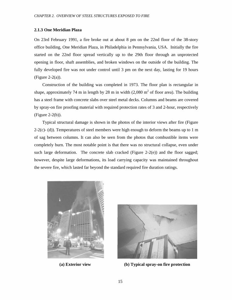
2.1.3 One Meridian Plaza
On 23rd February 1991, a fire broke out at about 8 pm on the 22nd floor of the 38-story
office building, One Meridian Plaza, in Philadelphia in Pennsylvania, USA. Initially the fire
started on the 22nd floor spread vertically up to the 29th floor through an unprotected
opening in floor, shaft assemblies, and broken windows on the outside of the building. The
fully developed fire was not under control until 3 pm on the next day, lasting for 19 hours
(Figure 2-2(a)).
Construction of the building was completed in 1973. The floor plan is rectangular in
shape, approximately 74 m in length by 28 m in width (2,080 m2 of floor area). The building
has a steel frame with concrete slabs over steel metal decks. Columns and beams are covered
by spray-on fire proofing material with required protection rates of 3 and 2-hour, respectively
(Figure 2-2(b)).
Typical structural damage is shown in the photos of the interior views after fire (Figure
2-2(c)- (d)). Temperatures of steel members were high enough to deform the beams up to 1 m
of sag between columns. It can also be seen from the photos that combustible items were
completely burn. The most notable point is that there was no structural collapse, even under
such large deformation. The concrete slab cracked (Figure 2-2(e)) and the floor sagged;
however, despite large deformations, its load carrying capacity was maintained throughout
the severe fire, which lasted far beyond the standard required fire duration ratings.
(a) Exterior view (b) Typical spray-on fire protection

CHAPTER 2. OVERVIEW OF STEEL STRUCTURES EXPOSED TO FIRE
16
(c) Interior view after fire (d) Interior view after fire
(e) Interior view after fire (f) Crack in concrete slab on 28th floor
Figure 2-2 Photos of One Meridian Plaza fire
(photo reference of USFA TR049)
2.1.4 World Trade Center Building 7
The 47-story steel commercial building located in the north region of the WTC complex
collapsed at 5:21 p.m. on 11th September 2001, about eight hours after the first aircraft struck
WTC tower 1 (NIST, 2004). The construction of the WTC building 7 was an expansion
project in 1987 using an existing structure of Con Ed Substation, which is a three-story steel
framed building originally built in 1967. The overall dimensions were approximately 100 m
(330 ft) long, 40 m (140 ft) width, and 190 m (610 ft) height. The column layout of the Con
Ed Substation and the additionally built upper portion of WTC 7 did not align and a series of
column transfer systems were constructed between Floors 5 and 7. The existing I-shaped
Con Ed Substation’s columns were braced with welded thick plates to the tops (between the
flange edges to make box sections) and strong diaphragm concrete slabs were built on Floors

CHAPTER 2. OVERVIEW OF STEEL STRUCTURES EXPOSED TO FIRE
17
5 and 7. Floors 8 through 45 had a typical framing plan with perimeter moment frames
(Figure 2-3).
It is reported that fires were observed on several floors (Floors 7, 8, 9, 11, 12 and 13)
(Figure 2-4) after 2 pm on the day; however, the exact time of the fire break-out and details
are uncertain. The building was damaged by falling debris from WTC tower 1 and 2 on the
south façade, which may have been a potential contribution to the building collapse.
However, the fires are more likely catalyst of this catastrophic event, given that collapse
occurred about six hours after the second tower (WTC 1) collapsed. There were two fuel
tanks located on Floor 5 for Con Ed’s emergency energy supply. It is uncertain if the fuel
was burned before the building collapse, because visual observation was impossible due to
the lack of windows on Floor 5. The scenario and mechanism of WTC 7 collapse is still
under investigation; however, the NIST (2004) studies report the probable sequence, which
are outlined and selectively quoted in the following description.
Figure 2-3 Floor plan and damages of WTC 7
(“June 2004 Progress Report on the Federal Building and Fire Safety Investigation of the World Trade Center Disaster, Appendix L- Interim Report on WTC 7,” NIST, 2004, Figure L-23c)
CHAPTER 2. OVERVIEW OF STEEL STRUCTURES EXPOSED TO FIRE
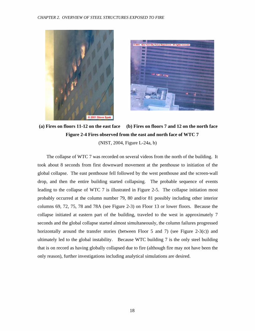
18
(a) Fires on floors 11-12 on the east face (b) Fires on floors 7 and 12 on the north face
Figure 2-4 Fires observed from the east and north face of WTC 7
(NIST, 2004, Figure L-24a, b)
The collapse of WTC 7 was recorded on several videos from the north of the building. It
took about 8 seconds from first downward movement at the penthouse to initiation of the
global collapse. The east penthouse fell followed by the west penthouse and the screen-wall
drop, and then the entire building started collapsing. The probable sequence of events
leading to the collapse of WTC 7 is illustrated in Figure 2-5. The collapse initiation most
probably occurred at the column number 79, 80 and/or 81 possibly including other interior
columns 69, 72, 75, 78 and 78A (see Figure 2-3) on Floor 13 or lower floors. Because the
collapse initiated at eastern part of the building, traveled to the west in approximately 7
seconds and the global collapse started almost simultaneously, the column failures progressed
horizontally around the transfer stories (between Floor 5 and 7) (see Figure 2-3(c)) and
ultimately led to the global instability. Because WTC building 7 is the only steel building
that is on record as having globally collapsed due to fire (although fire may not have been the
only reason), further investigations including analytical simulations are desired.
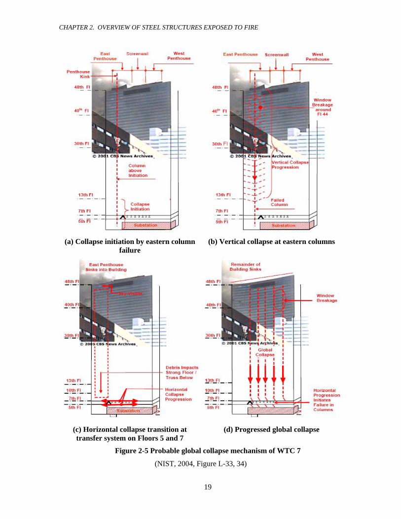
CHAPTER 2. OVERVIEW OF STEEL STRUCTURES EXPOSED TO FIRE
19
(a) Collapse initiation by eastern column
failure (b) Vertical collapse at eastern columns
(c) Horizontal collapse transition at transfer system on Floors 5 and 7
(d) Progressed global collapse
Figure 2-5 Probable global collapse mechanism of WTC 7
(NIST, 2004, Figure L-33, 34)
CHAPTER 2. OVERVIEW OF STEEL STRUCTURES EXPOSED TO FIRE
20
2.1.5 Windsor Building
On 12th February 2005, one of the most devastating fire disasters in the history of steel
structures occurred in the Windsor Building in Madrid, Spain. The fire broke out at about 11
pm on the 21st floor of the 32-story office building and quickly developed up to the top floor
by 1 am on the next day. The top ten floors were totally engulfed in flames and it gradually
spread to the lower floors. The fire reached the 17th floor by 2 am and about that time a
significant area of exterior cladding dropped. Upper floors partially collapsed at about 4 am
and the fire spread downward to 4th floor by 9 am. The fire was not under control until 2 pm
and the fire department declared the fire extinguished at 5 pm. The duration is between 18 to
20 hours.
The building is 32-stories and 106 m in height, and was completed in 1979. The floor
plan is rectangular in shape with approximately 40 m in length (7 bays with 5.6 m span) and
25 m in width (2 external 6.3 m bays and an internal 12.6 m core bay). The building is
composite steel and reinforced concrete (RC) structure (i.e., RC core and waffle slabs
supported by internal RC columns, internal steel beams, and perimeter steel columns).
Mechanical floors are located between 3rd and 4th floors and 16th and 17th floors. RC wall
girders (height 3750 mm, width 500 mm, and length 25 m) penetrate RC core in these
mechanical floors and the axial load of perimeter steel columns are transferred to the core by
the cantilevers of the wall girders. The perimeter steel columns are box shape in section and
consist of two welded channels (C shape sections), located every 1.8 m.
The building was constructed based on 1970’s Spanish design code, where the
specifications on fire protection were minimal. Unfortunately, the building was under
renovation to install new fire protection systems when the fire broke out. The installment
included sprinklers, fire protection of perimeter steel columns and interior beams, fire walls,
fire insulation of floors at perimeter cladding, and exterior stairs for evacuation. The
renovation was carried out from lower to upper floors. Fire protection of steel work had been
completed up to 17th floor, except for the 9th and part of 15th floor. No protection had been
installed on the 18th floor and higher. It is considered that the fire quickly spread to upper
floors through the uncompleted fire insulation of floors at the perimeter cladding. The fire
also developed slowly to lower stories, in a similar way, through partially incompleted fire
insulation of floors.
CHAPTER 2. OVERVIEW OF STEEL STRUCTURES EXPOSED TO FIRE
21
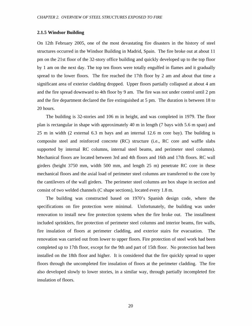
(a) Before fire (*1) (b) After fire (*2)
Figure 2-6 Exterior view of Windsor Building before and after the fire (*1) : Pedro Gonzalez (EFE) in report NILIM, 2005 (*2) : NILIM, 2005
Structural damage is significant at the top 11 stories, where fire protection had not been
installed to steelwork. Perimeter steel columns including exterior bays of waffle slabs almost
completely collapsed. However, the RC core maintained the strength and total collapse was
prevented (Figure 2-6). Lack of fire protection of the steel columns was critical to the partial
collapse. The probable collapse mechanism reported in NILIM (2005) is that (1) the steel
columns near the fire buckled due to material deterioration under elevated temperature, (2)
the axial load of the buckled columns were redistributed to adjacent structures, (3) the
number of deteriorated columns increased due to the developing fire, however, the waffle
slab worked as cantilever and prevented structural collapse, (4) the fire further spread and
waffle slabs reached their load carrying capacity as a cantilever for the extended supporting
area and collapsed, and (5) the floor collapse induced failure of other floors and waffle slabs
were ripped off at the connections to the core. It is certain that upper mechanical floor
between 16th and 17th floors provided enough redundancy to prevent progressive collapse,
resisting the impact of the partial collapse of upper floors and prevented further failure of
lower floors.
CHAPTER 2. OVERVIEW OF STEEL STRUCTURES EXPOSED TO FIRE
22
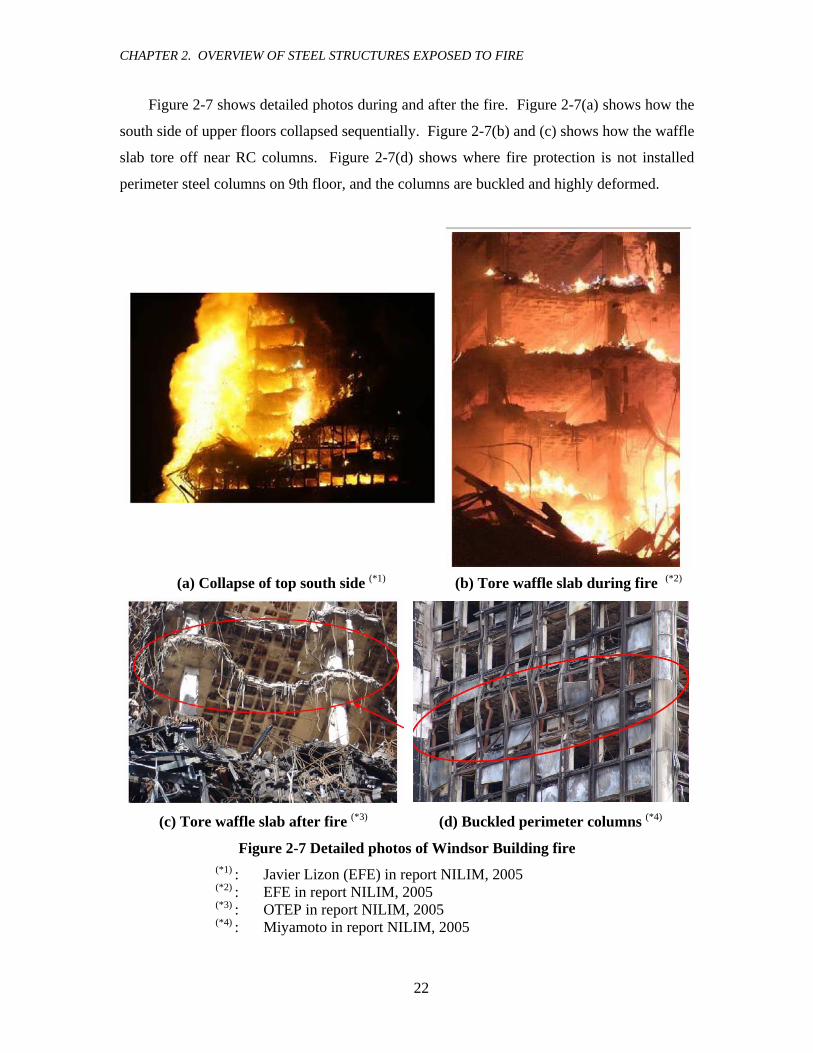
Figure 2-7 shows detailed photos during and after the fire. Figure 2-7(a) shows how the
south side of upper floors collapsed sequentially. Figure 2-7(b) and (c) shows how the waffle
slab tore off near RC columns. Figure 2-7(d) shows where fire protection is not installed
perimeter steel columns on 9th floor, and the columns are buckled and highly deformed.
(a) Collapse of top south side (*1) (b) Tore waffle slab during fire (*2)
(c) Tore waffle slab after fire (*3) (d) Buckled perimeter columns (*4)
Figure 2-7 Detailed photos of Windsor Building fire (*1) : Javier Lizon (EFE) in report NILIM, 2005 (*2) : EFE in report NILIM, 2005 (*3) : OTEP in report NILIM, 2005 (*4) : Miyamoto in report NILIM, 2005

CHAPTER 2. OVERVIEW OF STEEL STRUCTURES EXPOSED TO FIRE
23
2.1.6 Cardington Fire Test
In addition to review of past fire disasters of steel buildings, a large full-scale fire test
performed at Cardington in UK is briefly introduced in this section to further discuss the
actual behavior of steel structures under fires. The eight-story full-scale building fire test
(Figure 2-8) is unique compared to scales of other structural fire tests and provides interesting
information regarding characteristic behavior of steel frames under fires such as
redistribution of forces and thermally induced effects.
The test building was designed in accordance with British Standard or Eurocode and
targeted typical European steel buildings. The floor dimensions were 45 m in the length and
21 m in the width. Typical one-way steel decks were designed for composite floor structure
and design load was applied by using sand bags during the test. Six compartment fire tests
were performed in different floors and locations (Figure 2-9). Columns were covered with
fire insulations but beams were not. Some of the beams experienced elevated temperatures
greater than 1000 °C and large deformations (beam sagging); however, the building did not
even partially collapse. As steel strength at 1000 °C retains only about 5 % of strength at
ambient temperature, the composite effect played a significant role for the structural stability
under fires. This finding raised questions about current fire insulation design practice and
motivated steel composite floor design with only partial or even no fire insulation on
composite beams, although the interactive effect with other building components such as
compartment partitions must be carefully investigated for practical application. The ductile
deformation capacity of floor structure is remarkable; however the continuity and integrity of
the composite structures are to be further examined. This issue is especially important for US
design, because the generally good performance was attributed to slab reinforcement, which
is common in the UK but not usual in typical US construction practice. Despite the strength
of composite beams at elevated temperatures, columns were vulnerable to fires by losing
their load carrying capacity associated with local buckling. This was observed in tests of
columns located near beam-column connections that were unprotected. The columns and
connections were fully covered in the later tests. Further details about the Cardington Fire
Test can be found in several publications such as SCI (2000), Kirby (1997, 1998), Kirby et al.
(1996b, 1999) and Yang (2002).

CHAPTER 2. OVERVIEW OF STEEL STRUCTURES EXPOSED TO FIRE
24
(a) Frame overview (b) Deformed beams
Figure 2-8 Photos of the Cardington Fire Test
(Steel Construction Institute (SCI), (2000), “Fire Safety Design: A New Approach to Multi-Storey Steel-Framed Buildings,” SCI Publication P288, Figure A.1.1, B.3.18)
Figure 2-9 Floor framing and test locations
(SCI, 2000, Figure B.3.1)
CHAPTER 2. OVERVIEW OF STEEL STRUCTURES EXPOSED TO FIRE
25
2.1.7 Summary of Past Fire Disaster Review
Past fire disasters on steel buildings are reviewed in this section to learn from the observed
behavior of actual steel buildings under fires. Among the listed fire disasters, four major
events: Broadgate Phase 8, One Meridian Plaza, World Trade Center (WTC) building 7 and
Windsor Building, as well as Cardington eight-story full-scale fire test are reviewed in detail.
WTC tower 1 and 2 are not closely reviewed, because of the unique aspects of their design
and the terrorism attack. The most important point from this review is that no steel building
has totally collapsed by fire alone except perhaps WTC 7, which may have encountered some
physical damage that contributed to its collapse and experienced the extremely unusual
situation of not being attended to by fire fighters. This evidence illustrates the potential high
resistance of steel buildings under current design practice. Also, the superior performance of
steel beams observed in the cases of Broadgate Phase 8, One Meridian Plaza and Cardington
Fire Test should be highlighted. Some of the beams experienced elevated temperature
greater than 1000 °C without collapse, allowing large deformations with catenary actions.
On the other hand, steel columns have proven to be quite vulnerable in past fire disasters.
The Windsor Building partially collapsed in the upper stories, where fire insulation on the
columns was missing due to renovation. Also, local buckling with large distortions occurred
in the columns in the Cardington Fire Test, which must have significantly deteriorated the
axial strength. These observations are very helpful in understanding of characteristic
behavior of steel buildings under fires, although further careful investigations are necessary
to generalize and use the findings for structural fire design.
2.2 MECHANICAL PROPERTIES OF STEEL UNDER ELEVATED TEMPERATURES
2.2.1 Experimental Results
Evaluation of the mechanical properties of steel at elevated temperatures is essential for
analytical simulations of steel buildings exposed to fire. Large numbers of tests have been
carried out to investigate these properties; however, it is difficult to review these
experimental results comprehensively, given that some of the test results are contained in
internal institutional reports and are not easily accessible. In this section, some of the
available test results are reviewed and summarized to provide an overview of the basic
characteristics of behavior of steel at elevated temperatures.

CHAPTER 2. OVERVIEW OF STEEL STRUCTURES EXPOSED TO FIRE
26
Static material properties, specifically stress-strain curves, are reviewed in this section
and will be used again later in the studies presented in Chapters 3 to 5. Transient properties
such as rate dependence or creep strength are not specifically reviewed.
2.2.1.1 Experiments by Harmathy and Stanzak
Harmathy and Stanzak (1970) carried out tensile strength tests of structural steels at elevated
temperatures and provided complete stress-strain curves up to 10 % strain. This study was
among the first to examine large strain response of steel at high temperatures. In terms of the
history of structural fire engineering, this research is significant in the sense that the primary
focus is to provide useful information for design engineers who are concerned with assessing
the fire endurance of building elements. Structural steels manufactured in the United States
(ASTM A 36) were tested under 12 specified temperatures from 24 °C to 649 °C, and
Canadian structural steels (CSA G40.12) were tested under 13 specified temperatures from
24 °C to 704 °C. The minimum specified yield strength of ASTM A 36 and CSA G40.12 are
250 MPa (36 ksi) and 300 MPa (44 ksi), respectively. The measured chemical composition
from the specimens of these steels is shown in Table 2-2.
Tensile tests of these steels under elevated temperatures were performed under average
strain rates of 0.051 to 0.102 (min-1). The measured stress strain curves are shown in Figure
2-10. The relationships between the US and SI units are summarized in Appendix B. The
strength at 300 °C (572 °F) is greater than that at ambient temperature above 1 % strain. At
higher temperatures (≥ 400 °C or 572 °F), the strength is lower than that at ambient
temperatures. A significant strength drop is observed for tests conducted between 500 °C
(932 °F) and 600 °C (1112 °F). It is noteworthy that the explicit yield point and hardening
plateau, which is one of the distinct characteristics structural steel at ambient temperature, is
not clearly observed and nonlinear behavior is more significant at elevated temperatures.
Table 2-2 Chemical composition of steels by Harmathy and Stanzak (Wt%)
Steel C Mn P S Si Ni Cr Al ASTM A 36 0.19 0.71 0.007 0.03 0.09 - - - CSA G40.12 0.195 1.40 0.015 0.019 0.022 0.03 0.01 < 0.01

CHAPTER 2. OVERVIEW OF STEEL STRUCTURES EXPOSED TO FIRE
27
(a) ASTM A 36 steel
(b) CSA G40.12 steel
Figure 2-10 Stress-strain curves by Harmathy and Stanzak (1970)

CHAPTER 2. OVERVIEW OF STEEL STRUCTURES EXPOSED TO FIRE
28
2.2.1.2 Experiment by Skinner
Skinner (1972) performed comprehensive tests of Australian steels at elevated temperatures,
specifically focusing on information for prediction of behavior of structural steel members in
buildings. The tests covered not only mechanical properties such as modulus of elasticity,
tensile stress-strain properties, creep and thermal expansion, but also thermal properties such
as specific heat and thermal conductivity.
25.4mm (1 inch) thick plates were used for the tensile tests under specified constant
temperatures ranging from ambient temperature to 650 °C. Stress was measured under
controlled strain up to 5 % with six different strain rates from 1×10⁻⁵ (min-1) to 2×10⁻¹ (min-
1). The measured composition of the material is shown in Table 2-3 (AS A149 or AS
A186:250). Characteristic yield stress and tensile strength of the tested steel were 245 MPa
(35.5 ksi) and 487 MPa (70.6 ksi), respectively.
Table 2-3 Chemical composition of steel by Skinner (Wt%)
Steel C Mn P S Si Ni Cr Cu Al Mo AS A149 0.27 0.65 0.033 0.041 0.128 0.086 0.16 0.01 0.007 0.42
Figure 2-11 shows measured stress-strain curves with strain rate of 5×10⁻⁵ (min-1), which
is the slowest strain rate available for various temperatures from ambient temperature to 650
°C. The stresses were measured under controlled displacement up to strains of 0.05 (every
0.0025 up to 0.01 and every 0.005 up to 0.05). Stress-strain curves at selected temperatures;
ambient temperature, 300 °C, 400 °C, 500 °C and 600 °C, are plotted in Figure 2-11. The
strength at 300 °C is greater than that at ambient temperature above 1 % strain, whereas the
strength is lower than that at ambient temperatures at higher temperatures greater than 400 °C
(as also observed in the test by Harmathy and Stanzak (1970)).

CHAPTER 2. OVERVIEW OF STEEL STRUCTURES EXPOSED TO FIRE
29
0 0.01 0.02 0.03 0.04 0.050
50
100
150
200
250
300
350
400
450
500
Strain
Stre
ss (M
Pa)
RT300°C400°C500°C600°C
Figure 2-11 Stress-strain curves by Skinner (1972)
2.2.1.3 Experiments by DeFalco
DeFalco (1974) focused on and examined compressive properties of US structural steels at
elevated temperatures. Mechanical properties of three different types of structural steels
ASTM A36, A441, and A588, were tested at ambient temperature 21.1 °C (70 °F) and
elevated temperatures from 93.3 °C (200 °F) to 648.9 °C (1200 °F) at every 111.1 °C (200
°F). Tested specimens were round bars with 38.1 mm (1.5 inch) long and 12.7 mm (0.5 inch)
diameter.

CHAPTER 2. OVERVIEW OF STEEL STRUCTURES EXPOSED TO FIRE
30
(a) A 36 steel
(b) A 441 steel

CHAPTER 2. OVERVIEW OF STEEL STRUCTURES EXPOSED TO FIRE
31
(c) A 588 steel
Figure 2-12 Stress-strain curves by DeFalco (1974)
A total of 63 tests (21 for each type of steel) were performed and stress-strain curves
were obtained up to 1.5 % strain under a constant strain rate of 5×10⁻³ (min-1). The
characteristic yield strength of the steels varied depending on the shape and thickness. The
yield strength of A36 plates with thickness of 19.1 mm (3/4 inch) or less was 250 MPa (36
ksi) and those of A441 and A588 were 345 MPa (50 ksi). A36 is a common carbon steel,
whereas A441 and A588 are corrosion resistant high strength steels. The maximum
permissible chemical compositions of these types of steel are shown in Table 2-4. The
measured stress-strain curves of the three types of steel are shown in Figure 2-12. Three tests
were performed under a specified temperature for each type of steel. Mean values were used
to plot for the stress-strain curves in the figure.
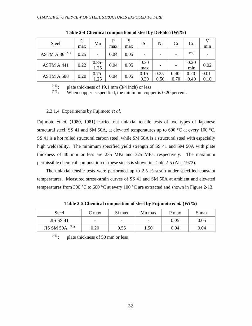
CHAPTER 2. OVERVIEW OF STEEL STRUCTURES EXPOSED TO FIRE
32
Table 2-4 Chemical composition of steel by DeFalco (Wt%)
Steel C max Mn P
max S
max Si Ni Cr Cu V min
ASTM A 36 (*1) 0.25 - 0.04 0.05 - - - (*2) -
ASTM A 441 0.22 0.85-1.25 0.04 0.05 0.30
max - - 0.20 min 0.02
ASTM A 588 0.20 0.75-1.25 0.04 0.05 0.15-
0.30 0.25-0.50
0.40-0.70
0.20-0.40
0.01-0.10
(*1) : plate thickness of 19.1 mm (3/4 inch) or less (*2) : When copper is specified, the minimum copper is 0.20 percent.
2.2.1.4 Experiments by Fujimoto et al.
Fujimoto et al. (1980, 1981) carried out uniaxial tensile tests of two types of Japanese
structural steel, SS 41 and SM 50A, at elevated temperatures up to 600 °C at every 100 °C.
SS 41 is a hot rolled structural carbon steel, while SM 50A is a structural steel with especially
high weldability. The minimum specified yield strength of SS 41 and SM 50A with plate
thickness of 40 mm or less are 235 MPa and 325 MPa, respectively. The maximum
permissible chemical composition of these steels is shown in Table 2-5 (AIJ, 1973).
The uniaxial tensile tests were performed up to 2.5 % strain under specified constant
temperatures. Measured stress-strain curves of SS 41 and SM 50A at ambient and elevated
temperatures from 300 °C to 600 °C at every 100 °C are extracted and shown in Figure 2-13.
Table 2-5 Chemical composition of steel by Fujimoto et al. (Wt%)
Steel C max Si max Mn max P max S max JIS SS 41 - - - 0.05 0.05
JIS SM 50A (*1) 0.20 0.55 1.50 0.04 0.04 (*1) : plate thickness of 50 mm or less

CHAPTER 2. OVERVIEW OF STEEL STRUCTURES EXPOSED TO FIRE
33
0 0.005 0.01 0.015 0.02 0.0250
50
100
150
200
250
300
350
Strain
Stre
ss (M
Pa)
SS41
RT300°C400°C500°C600°C
(a) SS 41 steel
0 0.005 0.01 0.015 0.02 0.0250
50
100
150
200
250
300
350
400
450
Strain
Stre
ss (M
Pa)
SM50
RT300°C400°C500°C600°C
(b) SM 50A steel
Figure 2-13 Stress-strain curves by Fujimoto et al. (1980, 81)
2.2.1.5 Experiments by Kirby and Preston
Kirby and Preston (1988) performed tensile tests of British steel under transient heating
conditions, where the mechanical load on a steel specimen was maintained at a constant and
the temperature increased under specified rates. This transient temperature-controlled testing

CHAPTER 2. OVERVIEW OF STEEL STRUCTURES EXPOSED TO FIRE
34
approach attempts to simulate the realistic behavior of structural steel under fire conditions,
given that the load on structures is almost always constant during fires and temperature
increases. In this testing procedure, stress-strain curves are translated from the strain-
temperature relationships. The steels tested were BS4360:1979 Grade 43A and 50B. The
characteristic strength was 255 MPa for Grade 43A (275 MPa according to BS4360:1986)
and 355 MPa for Grade 50B. The maximum permissible chemical compositions of these
steels are shown in Table 2-6.
Table 2-6 Chemical composition of steel by Kirby and Preston (Wt%)
Steel C max Si max Mn max P max S max BS Grade 43A 0.25 0.50 1.60 0.05 0.05 BS Grade 50B 0.23 0.50 1.50 0.05 0.05
Transient heating tests were carried out with the heating rate of 10 °C/min. The
translated stress-strain curves up to 2 % strain at ambient and elevated temperatures (300 °C
to 800 °C at every 100 °C) are shown in Figure 2-14. Comparing the results from their
transient tests with past steady-state experiments (mechanical loading under constant elevated
temperatures), they found that stress-strain relationships derived from these two types of
experiments were not significantly different.
0 0.005 0.01 0.015 0.020
50
100
150
200
250
300
Strain
Stre
ss (M
Pa)
Grade 43A
RT300°C400°C500°C600°C700°C800°C
(a) Grade 43A steel
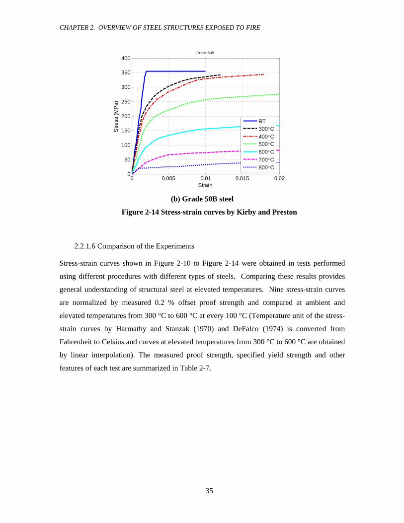
CHAPTER 2. OVERVIEW OF STEEL STRUCTURES EXPOSED TO FIRE
35
0 0.005 0.01 0.015 0.020
50
100
150
200
250
300
350
400
Strain
Stre
ss (M
Pa)
Grade 50B
RT300°C400°C500°C600°C700°C800°C
(b) Grade 50B steel
Figure 2-14 Stress-strain curves by Kirby and Preston
2.2.1.6 Comparison of the Experiments
Stress-strain curves shown in Figure 2-10 to Figure 2-14 were obtained in tests performed
using different procedures with different types of steels. Comparing these results provides
general understanding of structural steel at elevated temperatures. Nine stress-strain curves
are normalized by measured 0.2 % offset proof strength and compared at ambient and
elevated temperatures from 300 °C to 600 °C at every 100 °C (Temperature unit of the stress-
strain curves by Harmathy and Stanzak (1970) and DeFalco (1974) is converted from
Fahrenheit to Celsius and curves at elevated temperatures from 300 °C to 600 °C are obtained
by linear interpolation). The measured proof strength, specified yield strength and other
features of each test are summarized in Table 2-7.

CHAPTER 2. OVERVIEW OF STEEL STRUCTURES EXPOSED TO FIRE
36
Table 2-7 Comparison of steel experiments at elevated temperatures
Steel Measured
yF (MPa) Specified
yF (MPa) Researcher Testing procedure maxε (*1) maxT (*2)
ASTM A 36 300 250 650 CSA G40.12 350 300
Harmathy and Stanzak (1970)
Steady-state (*3)
Tensile 10 700
AS A 149 236 245 Skinner (1972)
Steady-state (*3)
Tensile 5 650
ASTM A 36 295 250 ASTM A 441 385 345
DeFalco (1974)
Steady-state (*3)
Compressive < 2 650
JIS SS 41 245 235 JIS SM 50A 356 325
Fujimoto et al. (1980, 1981)
Steady-state (*3)
Tensile 2.5 600
BS Gr. 43A 255 255 BS Gr. 50B 355 355
Kirby and Preston (1988)
Transient (*4) Tensile 2 800
(*1) : upper limit of measured strain (%) (*2) : upper limit of measured temperature (°C) (*3) : fixed temperature (*4) : fixed load
These stress-strain curves up to 2.5 % strain are compared in Figure 2-15. Difference of
these responses is relatively small up to 500 °C, while significant difference is observed at
600 °C. The two tests conducted by DeFalco agree well each other at any temperatures.
Also the two tests by by Fujimoto et al., and Kirby and Preston agree. This fact is true even
at 600 °C, where overall results are relatively scattered. On the other hand, the two tests by
Harmathy and Stanzak are relatively different. This is probably because Harmathy and
Stanzak tested steels manufactured in two different countries (the US and Canada), whereas
the other studies tested steel from only one country. Skinner and Fujimoto et al. used similar
testing approaches (i.e., tests under specified constant temperatures); however their results
are not necessarily closer than others.
Statistical information regarding the steel strength at elevated temperatures is
investigated based on these data and is shown in Chapter 5.

CHAPTER 2. OVERVIEW OF STEEL STRUCTURES EXPOSED TO FIRE
37
0 0.005 0.01 0.015 0.02 0.0250
0.2
0.4
0.6
0.8
1
1.2
Strain
Stre
ss /
Yie
ld s
tress
RT
ASTM A36 (Harmathy)CSA G40AS A149ASTM A36 (DeFalco)ASTM A441JIS SS41JIS SM50ABS Gr43ABS Gr50B
(a) Ambient temperature
0 0.005 0.01 0.015 0.02 0.0250
0.5
1
1.5
Strain
Stre
ss /
Yie
ld s
tress
300°C
0 0.005 0.01 0.015 0.02 0.0250
0.2
0.4
0.6
0.8
1
1.2
Strain
Stre
ss /
Yie
ld s
tress
400°C
(b) 300°C (c) 400°C
0 0.005 0.01 0.015 0.02 0.0250
0.2
0.4
0.6
0.8
1
Strain
Stre
ss /
Yie
ld s
tress
500°C
0 0.005 0.01 0.015 0.02 0.0250
0.1
0.2
0.3
0.4
0.5
0.6
Strain
Stre
ss /
Yie
ld s
tress
600°C
(d) 500°C (e) 600°C
Figure 2-15 Comparison of stress-strain curves in experiments

CHAPTER 2. OVERVIEW OF STEEL STRUCTURES EXPOSED TO FIRE
38
2.2.2 Equations of Stress-strain Curves
In order to use the experimentally measured stress-strain data for design analysis, stress-
strain relationships need to be formulated in practical and continuous functions. The
structural steel tests at elevated temperatures shown in the previous sections were carried out
in five different countries; Canada, Australia, the US, Japan and the UK. Design standards
for steel structures against fires are different in these countries with different levels of
development. Design equations of the steel stress-strain curves at elevated temperatures in
the design standards are compared and discussed.
2.2.2.1 Eurocode Stress-strain Curves
At present, the Eurocode is the most developed design standard for structural fire design.
Each of following nine parts of the Eurocode contains significant coverage of structural fire
engineering:
EN 1991 Eurocode 1 Basis of design and actions on structures
EN 1992 Eurocode 2 Design of concrete structures
EN 1993 Eurocode 3 Design of steel structures
EN 1994 Eurocode 4 Design of composite steel and concrete structures
EN 1995 Eurocode 5 Design of timber structures
EN 1996 Eurocode 6 Design of masonry structures
EN 1997 Eurocode 7 Geotechnical design
EN 1998 Eurocode 8 Design provisions for earthquake resistance of structures
EN 1999 Eurocode 9 Design of aluminum alloy structures
Guidance on fire simulations, and the design of concrete and steel structures for fire
conditions are contained in Eurocode 1 (EC1, 2002), Eurocode 2 (EC2, 1993), and Eurocode
3 (EC3, 2003), respectively. Relationships describing time and gas temperatures in flashover
fires are defined in EC1 as functions of influential factors, such as fuel load, geometry of fire
compartment, openings and firefighting activities. The described relationships allow
engineers to estimate temperatures of gas in fire compartments and consequently
temperatures of structural steel depending on the type and thickness of fire insulation.

CHAPTER 2. OVERVIEW OF STEEL STRUCTURES EXPOSED TO FIRE
39
Both conceptual and detailed descriptions regarding strength calculations of steel
structures during fires are included in EC3. Design equations for stress-strain curves of
structural steel at elevated temperatures are also defined in EC3. The idealized curves consist
of three regions; elastic, transition, and perfectly-plastic. Figure 2-16 shows the shape and
key parameters of the stress-strain curves, where ( )E T , ( )pF T and ( )yF T are modulus of
elasticity, proportional-limit stress and yield stress, respectively. These key parameters are
explicit functions of temperature of T . ( )p Tε and ( )y Tε are strains corresponding to
( )pF T and ( )yF T .
(a) Stress-strain curves (b) Key parameters
(c) Reduction factors
Figure 2-16 Stress-strain curves defined by EC3

CHAPTER 2. OVERVIEW OF STEEL STRUCTURES EXPOSED TO FIRE
40
Reduction factors for the modulus of elasticity, stress at proportional-limit and yielding
with respect to temperatures are shown in Figure 2-16(c). These are defined as proportions
of values at elevated temperatures to those at ambient temperature as shown in Equation (2.1)
, where 0E , 0pF and 0yF are modulus of elasticity, proportional-limit stress and yield stress
at ambient temperature, respectively.
0
( )( )EE TK TE
= , 0
( )( ) p
pp
F TK T
F= , and
0
( )( ) y
yy
F TK T
F= (2.1)
Stress-strain curves at elevated temperatures are shown in Figure 2-16(a). These are
obtained by substituting the reduction factors into the equations defined in EC3. The
significant drop of strength between 400 °C and 700 °C, which was observed in experimental
results, are represented in these curves.
2.2.2.2 AS4100 Stress-strain Curves
The Australian Standard for steel structures, AS4100 (ABCB, 1998), contains documentation
about design of steel structures under fire conditions; however, it is less comprehensive than
the Eurocode. Description in AS4100 about the mechanical properties of structural steel at
elevated temperatures is limited to yield stress and modulus of elasticity (i.e., no proportional
limit stress). Reduction factors of these values are defined as proportions of values at
elevated temperatures to those at ambient temperature in similar way used in Eurocode. The
defined reduction factors of the modulus of elasticity and yield strength are shown in Figure
2-17(a).
Since there is no definition about stress-strain curves considering highly nonlinear
behavior of steel at high temperatures, it is interpreted that characteristic bilinear stress-strain
curves at ambient temperature is used at elevated temperatures. Simple structural analysis for
fires can be performed by using these degraded modulus of elasticity and yield strength.
Assuming perfect-plastic bilinear, stress-strain curves under elevated temperature by AS4100
are shown in Figure 2-17(b). These curves can be useful for simple member-based strength
evaluation; however, they do not represent realistic behavior of structural steel and are not
appropriate be used in advanced analytical simulations.
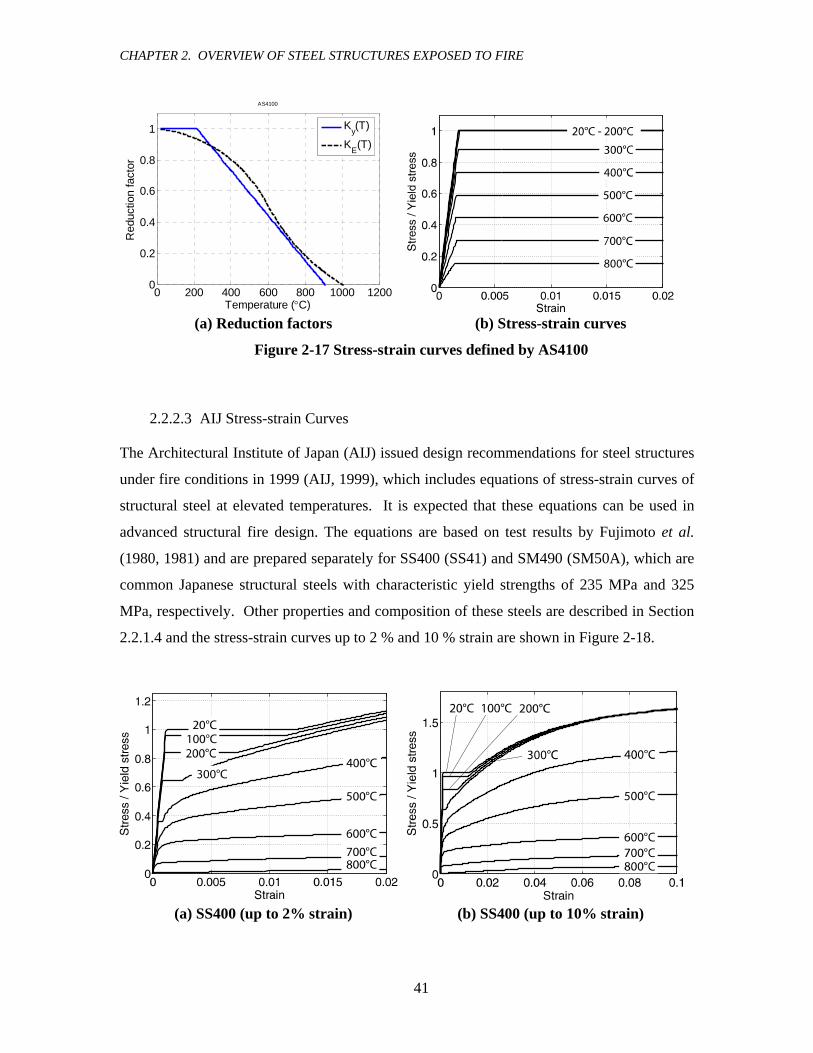
CHAPTER 2. OVERVIEW OF STEEL STRUCTURES EXPOSED TO FIRE
41
0 200 400 600 800 1000 12000
0.2
0.4
0.6
0.8
1
AS4100
Temperature (°C)
Red
uctio
n fa
ctor
Ky(T)
KE(T)
(a) Reduction factors (b) Stress-strain curves
Figure 2-17 Stress-strain curves defined by AS4100
2.2.2.3 AIJ Stress-strain Curves
The Architectural Institute of Japan (AIJ) issued design recommendations for steel structures
under fire conditions in 1999 (AIJ, 1999), which includes equations of stress-strain curves of
structural steel at elevated temperatures. It is expected that these equations can be used in
advanced structural fire design. The equations are based on test results by Fujimoto et al.
(1980, 1981) and are prepared separately for SS400 (SS41) and SM490 (SM50A), which are
common Japanese structural steels with characteristic yield strengths of 235 MPa and 325
MPa, respectively. Other properties and composition of these steels are described in Section
2.2.1.4 and the stress-strain curves up to 2 % and 10 % strain are shown in Figure 2-18.
(a) SS400 (up to 2% strain) (b) SS400 (up to 10% strain)

CHAPTER 2. OVERVIEW OF STEEL STRUCTURES EXPOSED TO FIRE
42
(c) SM490 (up to 2% strain) (d) SM490 (up to 10% strain) Figure 2-18 Stress-strain curves defined by AIJ
The stress-strain curves of these steels at elevated temperatures are composed of three
portions; the elastic portion, the hardening plateau portion, and the strain hardening portion.
The hardening plateau portion gradually reduces under elevated temperatures and completely
disappears at 500 °C (see Figure 2-18). The equations, which define these curves, are as
follows:
{ }1 2( , ) max ( , ), ( , )T T Tσ ε σ ε σ ε= (2.2)
where ( , )Tσ ε is defined stress under temperature T and strain ε , and:
{ }1( , ) min ( ) , ( )pT E T Tσ ε ε σ= (2.3)
( )( )( ){ } ( )
2 2 3 23 2
( ) ( ) ( )( , )1 0.051 ( ) ( ) ( )
C C
C C
E T E T E TTE T E T T
ε εσ εεε σ
−= +
++ − (2.4)
( )E T and ( )p Tσ are modulus of elasticity and stress at proportional limit at T ,
respectively.
6 2( ) 210,000 (1 10 )E T T−= × − (MPa) (2.5)
6 2( ) 240 (1 4 10 )p T Tσ −= × − × (MPa) if 500T ≤ °C and SS400 (2.6)

CHAPTER 2. OVERVIEW OF STEEL STRUCTURES EXPOSED TO FIRE
43
6 2( ) 330 (1 4 10 )p T Tσ −= × − × (MPa) if 500T ≤ °C and SM490 (2.7)
( ) 0p Tσ = (MPa) if 500T > °C (2.8)
( )CE T and ( )C Tσ are given in Table 2-8. Values can be linearly interpolated for each
table.
Table 2-8 Coefficients in AIJ equations for stress-strain curves
SS400 SS400 SM490 SM490
T (°C)
( )CE T(MPa)
T (°C)
( )C Tσ(MPa)
T (°C)
( )CE T(MPa)
T (°C)
( )C Tσ(MPa)
0 4500 0 190 0 4500 0 270
300 5200 300 160 300 4500 320 270
600 750 500 90 600 600 600 110
1000 0 750 0 1000 0 750 0
The concept of reduction factors of steel properties at elevated temperatures is not
explicitly adopted in AIJ equations, rather the precise stress-strain curves are defined instead.
Reduction ratios of key parameters are derived from these stress-strain curves (see Figure
2-19). In order to compare stress-strain equations in AIJ with those in other design standards,
( )yK T and ( )pK T are defined here as the ratios of stresses at 2 % strain and on the
hardening plateau at temperature T , with respect to the characteristic yield strength.
Different values of ( )yK T are prepared for SS400 and SM490 steel, while the values of
( )pK T are shared between them (see Eqs. (2.6) to (2.8)). ( )EK T is a proportion of modulus
of elasticity at T to that at ambient temperature, as given in Eq. (2.5).

CHAPTER 2. OVERVIEW OF STEEL STRUCTURES EXPOSED TO FIRE
44
0 200 400 600 800 1000 12000
0.2
0.4
0.6
0.8
1
1.2
Temperature (°C)
Red
uctio
n fa
ctor
Ky(T)SS400Ky(T)SM490Kp(T)KE(T)
Figure 2-19 Reduction ratios in the stress-strain curves defined by AIJ
2.2.2.4 AISC Stress-strain Curves
Structural fire engineering toward performance-based design is still in a developing stage in
the United States. Structural Design for Fire Conditions has been recently included in an
appendix of the Specification for Structural Steel Buildings in the US design standard of steel
structures by American Institute of Steel Construction (AISC-LRFD, 2005). The
specification describes two types of analytical approaches, referred to as the Advanced
Method and the Simple Method. Rigorous structural and thermal analyses are required for the
advanced method, while design equations at ambient temperatures are used for the simple
method. In these AISC methods, the degradation ratios of the material properties such as
modulus of elasticity and yield stress under elevated temperatures are adopted from Eurocode
3 (EC3, 1995). The degraded material properties are substituted into the equations at ambient
temperature and the strength of the structural members under fire conditions is individually
evaluated in this simple method. Other than the material deterioration ratios, there is no
stress-strain curve defined for structural steel under elevated temperatures. This approach is
similar in concept to the Australian Standard, AS4100, described in Section 2.2.2.2.
Therefore, it can be interpreted that the characteristic bilinear stress-strain curve of structural
steel at ambient temperature is also assumed for those under elevated temperatures (Figure
2-20). Since the reduction factors are adopted directly from EC3, Figure 2-20(a) is the same
as Figure 2-16(a) fitted to the elastic modulus and the yield strength, and Figure 2-20(b) is a
bilinear approximation of the stress-strain curves previously shown in Figure 2-16(b).

CHAPTER 2. OVERVIEW OF STEEL STRUCTURES EXPOSED TO FIRE
45
0 200 400 600 800 1000 12000
0.2
0.4
0.6
0.8
1
Temperature (°C)
Red
uctio
n fa
ctor
Ky(T)
KE(T)
(a) Reduction factors (b) Stress-strain curves Figure 2-20 Stress-strain curves defined by AISC
2.2.2.5 Comparison of the Equations of Stress-strain Curves
The equations of the stress-strain curves of structural steel at elevated temperatures, defined
in or interpreted from the four design standards, EC3, AS4100, AIJ (SM490), and AISC, are
compared at ambient and elevated temperatures up to 1000 °C at every 100 °C in Figure
2-21. The stress-strain curves obtained through experiments and introduced in Section 2.2.1
are also superimposed in the figures at ambient temperature and 300 °C to 800 °C. These
curves are normalized by the characteristic yield strength for the equations and the measured
yield strength at the test results. Temperatures less than 400 °C are typically not important in
structural fire engineering, because the overall strength degradation is fairly modest up to this
temperature. Comparing the equations and test results between 400 °C and 600 °C, it is
observed that the Eurocode equation is close to or slightly lower than the mean of the test
results and is the best representative of actual steel properties at elevated temperatures among
these four equations. It is unfortunate that test results at more than 600 °C are not obtained
and comparison between the test data and equations is not possible.
The perfectly plastic bilinear stress-strain curves from AS4100 and AISC do not
represent highly nonlinear stress-strain response of steel at elevated temperatures. In
addition, equations from AS4100 are conservative at 300 °C to 500 °C, while they are
unconservative at 700 °C and 800 °C. The AIJ equations more precisely represent the shape
of the stress-strain curves. The equations best fit the test results at ambient temperature,
properly taking into account strain hardening. However, the strength of the AIJ equations is

CHAPTER 2. OVERVIEW OF STEEL STRUCTURES EXPOSED TO FIRE
46
very conservative at higher temperatures, such as 500 °C and higher. This is because the
target stress-strain curves to define the AIJ equations are approximately mean minus three
times the standard deviation of tested stress-strain curves. The safety margin of structural
design for highly unknown building behavior under fire conditions is taken into account in
the predictive equations. This may be an effective approach to assure the safety; however, it
may not fit with the concept of Load and Resistance Factor Design (LRFD), where limit-state
strength and nominal load are simulated as accurately as possible and structural safety is
evaluated by taking into account the effect of uncertainties with the load and resistance
factors.
0 0.01 0.02 0.03 0.040
0.2
0.4
0.6
0.8
1
1.2
Stre
ss /
Yie
ld s
tress
Strain
20°C
EC3ASAIJAISCTest
(a) Ambient temperature (20 °C)
0 0.01 0.02 0.03 0.040
0.2
0.4
0.6
0.8
1
1.2
Stre
ss /
Yie
ld s
tress
Strain
100°C
0 0.01 0.02 0.03 0.040
0.2
0.4
0.6
0.8
1
1.2
Stre
ss /
Yie
ld s
tress
Strain
200°C
(b) 100 °C (c) 200 °C
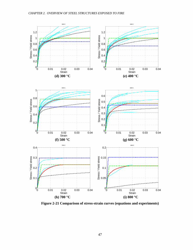
CHAPTER 2. OVERVIEW OF STEEL STRUCTURES EXPOSED TO FIRE
47
0 0.01 0.02 0.03 0.040
0.2
0.4
0.6
0.8
1
1.2S
tress
/ Y
ield
stre
ss
Strain
300°C
0 0.01 0.02 0.03 0.040
0.2
0.4
0.6
0.8
1
1.2
Stre
ss /
Yie
ld s
tress
Strain
400°C
(d) 300 °C (e) 400 °C
0 0.01 0.02 0.03 0.040
0.2
0.4
0.6
0.8
1
Stre
ss /
Yie
ld s
tress
Strain
500°C
0 0.01 0.02 0.03 0.040
0.1
0.2
0.3
0.4
0.5
0.6S
tress
/ Y
ield
stre
ss
Strain
600°C
(f) 500 °C (g) 600 °C
0 0.01 0.02 0.03 0.040
0.1
0.2
0.3
0.4
Stre
ss /
Yie
ld s
tress
Strain
700°C
0 0.01 0.02 0.03 0.040
0.05
0.1
0.15
0.2
Stre
ss /
Yie
ld s
tress
Strain
800°C
(h) 700 °C (i) 800 °C
Figure 2-21 Comparison of stress-strain curves (equations and experiments)
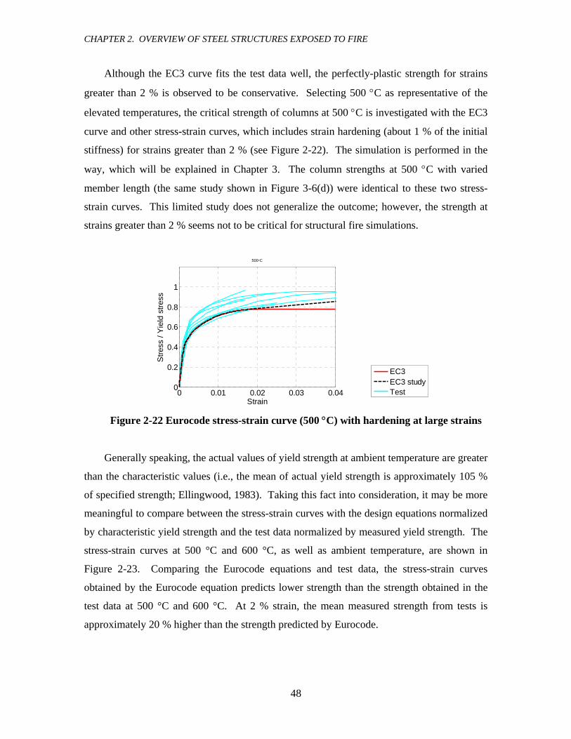
CHAPTER 2. OVERVIEW OF STEEL STRUCTURES EXPOSED TO FIRE
48
Although the EC3 curve fits the test data well, the perfectly-plastic strength for strains
greater than 2 % is observed to be conservative. Selecting 500 °C as representative of the
elevated temperatures, the critical strength of columns at 500 °C is investigated with the EC3
curve and other stress-strain curves, which includes strain hardening (about 1 % of the initial
stiffness) for strains greater than 2 % (see Figure 2-22). The simulation is performed in the
way, which will be explained in Chapter 3. The column strengths at 500 °C with varied
member length (the same study shown in Figure 3-6(d)) were identical to these two stress-
strain curves. This limited study does not generalize the outcome; however, the strength at
strains greater than 2 % seems not to be critical for structural fire simulations.
0 0.01 0.02 0.03 0.040
0.2
0.4
0.6
0.8
1
Stre
ss /
Yie
ld s
tress
Strain
500°C
EC3EC3 studyTest
Figure 2-22 Eurocode stress-strain curve (500 °C) with hardening at large strains
Generally speaking, the actual values of yield strength at ambient temperature are greater
than the characteristic values (i.e., the mean of actual yield strength is approximately 105 %
of specified strength; Ellingwood, 1983). Taking this fact into consideration, it may be more
meaningful to compare between the stress-strain curves with the design equations normalized
by characteristic yield strength and the test data normalized by measured yield strength. The
stress-strain curves at 500 °C and 600 °C, as well as ambient temperature, are shown in
Figure 2-23. Comparing the Eurocode equations and test data, the stress-strain curves
obtained by the Eurocode equation predicts lower strength than the strength obtained in the
test data at 500 °C and 600 °C. At 2 % strain, the mean measured strength from tests is
approximately 20 % higher than the strength predicted by Eurocode.

CHAPTER 2. OVERVIEW OF STEEL STRUCTURES EXPOSED TO FIRE
49
0 0.01 0.02 0.03 0.040
0.5
1
1.5S
tress
/ Y
ield
stre
ss
Strain
20°C
EC3ASAIJAISCTest
(a) Ambient temperature (20 °C)
0 0.01 0.02 0.03 0.040
0.2
0.4
0.6
0.8
1
Stre
ss /
Yie
ld s
tress
Strain
500°C
0 0.01 0.02 0.03 0.040
0.2
0.4
0.6
0.8
Stre
ss /
Yie
ld s
tress
Strain
600°C
(b) 500 °C (c) 600 °C
Figure 2-23 Comparison of normalized stress-strain curves (equations and experiments)
2.2.3 Experiments by JISF
The Japan Iron and Steel Federation (JISF) experimentally investigated tensile stress-strain
relationships of Japanese standard steels under ambient and elevated temperatures (20 °C and
300 °C to 800 °C). Six different types of steel were examined. Five sets (five different
supplies) of test data are included for each type of steel and each set contains stress-strain
curves under different temperatures (ambient and elevated temperatures from 300 °C to 800
°C at every 100 °C). The total number of tests is 280.
Figure 2-24 shows comparison of stress-strain curves from the JISF test data and curves
by EC3 and AIJ at 500 °C, 600 °C, and 700 °C. As is also observed in the comparative study
discussed in the previous section (2.2.2.5), the EC3 curves agree better with the test data than
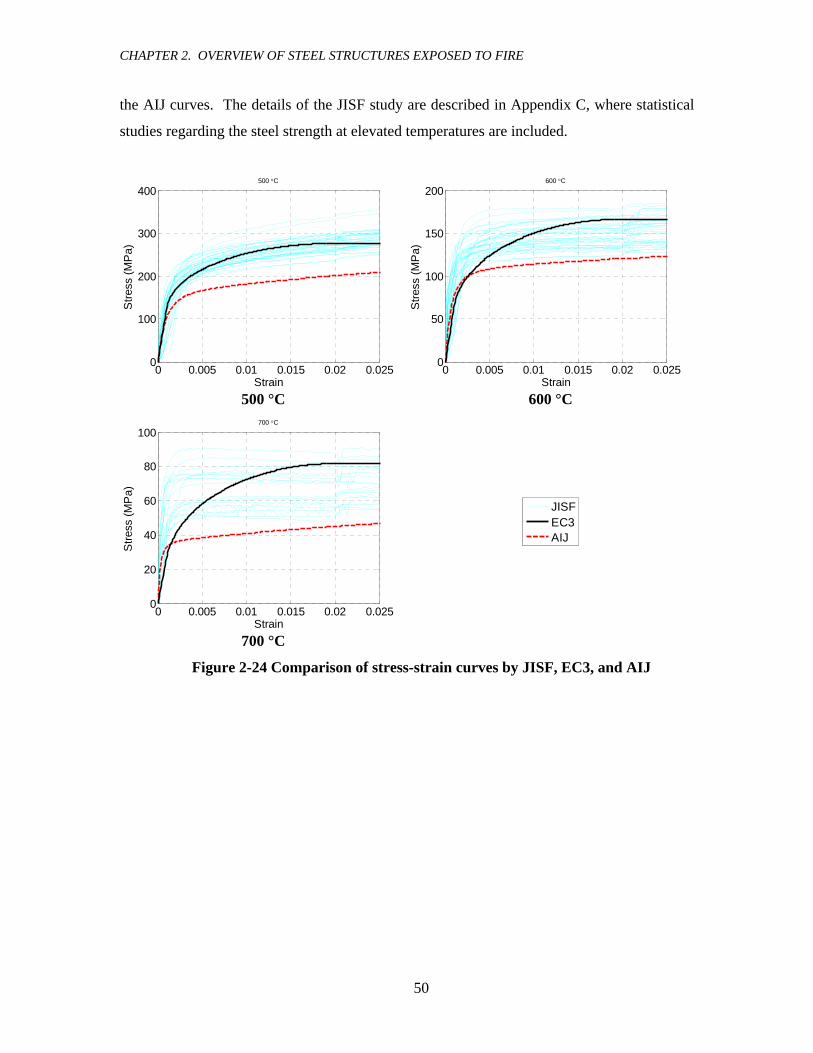
CHAPTER 2. OVERVIEW OF STEEL STRUCTURES EXPOSED TO FIRE
50
the AIJ curves. The details of the JISF study are described in Appendix C, where statistical
studies regarding the steel strength at elevated temperatures are included.
0 0.005 0.01 0.015 0.02 0.0250
100
200
300
400
Stre
ss (M
Pa)
Strain
500 °C
0 0.005 0.01 0.015 0.02 0.0250
50
100
150
200
Stre
ss (M
Pa)
Strain
600 °C
500 °C 600 °C
0 0.005 0.01 0.015 0.02 0.0250
20
40
60
80
100
Stre
ss (M
Pa)
Strain
700 °C
JISFEC3AIJ
700 °C
Figure 2-24 Comparison of stress-strain curves by JISF, EC3, and AIJ

51
CHAPTER 3 ANALYSIS OF INDIVIDUAL MEMBERS
3 ANALYSIS OF INDIVIDUAL MEMBERS
Takagi, J., Deierlein, G.G. “Strength Design Criteria for Steel Members at Elevated Temperatures,” Journal of Constructional Steel Research, (in press) See Appendix A for further studies on behavior of individual members at elevated temperatures.
3.1 SUMMARY
Design equations for structural steel members at elevated (fire) temperatures are evaluated
through comparisons to nonlinear finite element simulations. The study includes
comparative analyses of the American Institute of Steel Construction (AISC) and European
Committee for Standardization (CEN) design provisions for laterally unsupported I-shaped
columns, beams, and beam-columns at temperatures between ambient to 800 oC. The
Eurocode 3 provisions are shown to predict the simulated finite element results within about
10 % to 20 %. On the other hand, the AISC specification predicts strengths that are up to
twice as large (unconservative) as the simulated results. The discrepancies are largest for
members of intermediate slenderness and temperatures above 300 oC. Modifications to the
AISC equations are proposed that provide improved accuracy with calculated strengths
typically within 20 % to 30 % of the simulated results. Limitations of the member-based
assessments and future research and development needs for structural fire engineering are
discussed.
3.2 INTRODUCTION
While the basic concepts for structural fire engineering are well established, explicit
assessment of structural response to fires is uncommon in engineering practice. Instead,
building codes and design practice have traditionally relied on prescriptive requirements to
provide adequate structural fire-resistance in building structures. In steel-framed structures,
this is typically accomplished through thermal insulation requirements that are validated by

CHAPTER 3. ANALYSIS OF INDIVIDUAL MEMBERS
52
fire endurance tests. Such approaches may work well for routine design, however, the lack of
alternative methods to establish structural performance by calculation impedes the design of
structures where the prescriptive methods fall short of providing effective solutions.
Recently, the situation is changing with the publication of standards to calculate structural
fire resistance in a manner similar to how other strength limit states are evaluated. For
example, the Eurocode 3 (EC3, 2003) standard includes detailed provisions to establish fire
loads and evaluate their effects on steel structures. The latest edition of the Specification for
Structural Steel Buildings in the American Institute of Steel Construction (AISC, 2005)
includes a new appendix entitled, Structural Design for Fire Conditions, which provides
guidance and criteria to evaluate the structural resistance of steel building components at
elevated temperatures.
The EC3 and AISC standards for steel structures both follow an approach whereby the
structural resistance to gravity and other loads is calculated with the steel members at an
assumed elevated temperature. Each standard permits this evaluation through either an
“advanced” or “simple” method, where the former requires rigorous structural and thermal
simulations and the latter method is accomplished through member-based strength limit state
checks. The member-based approaches are similar to conventional checks made at ambient
temperatures. In the AISC specification, for example, the member design strength equations
are essentially the same as those for ambient temperatures, except that the input yield
strength and elastic modulus of the steel are reduced based on the assumed elevated
temperature. While the AISC method is straightforward and easy to implement, its accuracy
has not been thoroughly verified. On the other hand, the structural fire provisions of EC3
have been published in codified form since the early 1990’s and have been reviewed and
modified since their first publication.
The objective of this study is to provide a critical assessment of the AISC and EC3
member strength equations through a comparison to results of detailed finite element
simulations at elevated temperatures. The assessment includes laterally unsupported
columns, beams, and beam-columns of bi-symmetric I-shaped steel sections with idealized
loading and boundary conditions. The simulations employ three dimensional shell finite
element models that capture inelastic yielding, overall and local buckling, and non-uniform
torsion effects. The column strengths are evaluated in terms of critical axial load applied to a
pin-ended column with initial geometric imperfections that represent fabrication tolerances.
The beam strengths are evaluated in terms of critical bending moments, which are applied

CHAPTER 3. ANALYSIS OF INDIVIDUAL MEMBERS
53
about the major-axis at the ends of a simply supported beam that is laterally unsupported and
susceptible to lateral-torsional buckling. Results are then compared for the combined effects
of axial compression and bending in beam-columns. The assessment covers a range of
design conditions by parametrically varying the elevated temperatures and member lengths.
Most of the analyses are for members of Grade 50 steel (yield strength of yF = 345 MPa)
with selected study of Grade 36 ( yF = 250 MPa) steel.
As will be demonstrated, the AISC strength equations at elevated temperatures are
unconservative, and alternative strength equations are proposed. The proposed equations are
similar in format to the
AISC provisions, thus maintaining practicality for design. Beyond the immediate
benefit of the improved design equations, this research provides fundamental information to
improve the understanding of structural steel members under fire conditions.
3.3 BASIS OF MEMBER STRENGTH EVALUATIONS
Assessment of structural safety to fire hazards can generally be categorized into three stages.
The first stage entails characterization of fire initiation and development, which can be done
either through direct simulation or through parametric time-temperature models of
compartment gas temperatures. The second stage involves heat transfer calculations to
evaluate temperatures in structural members, considering insulation and other factors that
affect heat transfer. The third stage is to assess structural behavior under elevated
temperatures, including the effects of both thermal expansion and degradation of material
properties. The assessments made within each of these three stages are generally treated as
conditionally independent, where it is assumed that structural behavior does not impact heat
transfer or fire development and heat transfer does not impact fire development. While there
are situations where the assumption of conditional independence does not hold (e.g., where
structural deformations may damage fire compartments, which in turn affects fire
development), in most cases the conditional independence is a reasonable assumption. This
assumption greatly simplifies the assessment since the analyses in each stage can be done
separately and without interaction. This line of reasoning is implicit in the structural fire
assessment presented herein (and in the AISC and EC3 design provisions), where the
elevated steel temperatures are treated as input to the structural assessment and calculated
independently.

CHAPTER 3. ANALYSIS OF INDIVIDUAL MEMBERS
54
In this study, it is assumed that the elevated temperature of the steel members is known
(or can be determined) and used to evaluate the strength limit state of individual members
under the combined effects of elevated temperature and applied loads. In concept, the
strength limit state can then be evaluated either by (1) calculating the critical temperature
(intensity and distribution) that the member can sustain under the given loads, or (2)
calculating the strength (load resistance) of a member under a specified temperature. The
former approach, referred to herein as the “temperature approach”, is more representative of
the actual fire conditions, where the temperature increases as the while the applied gravity
loads are constant. The latter approach (termed the “load approach”) is simpler to implement
in nonlinear analysis and fits more naturally in existing formats for structural assessment,
where member design equations or simulation tools (e.g., nonlinear analysis) are used to
assess the critical loads based on the specified temperature-dependent material properties.
Although material nonlinear analyses are, in concept, load path dependent, for monotonically
increasing gravity loads and temperatures of individual members, it is reasonable to assume
that the critical limit state calculated following a “temperature approach” and “load
approach” should be similar.
Figure 3-1 Comparison of temperature and load control analyses
The authors have confirmed this assumption by conducting finite element analyses of
individual members with fixed loads and variable temperature and vice versa. Shown in
Figure 3-1 is an example of one such analysis, where the critical combinations of temperature
and strength for a column are obtained by both approaches. This example is for a W14×90

CHAPTER 3. ANALYSIS OF INDIVIDUAL MEMBERS
55
Grade 50 column (W360×134; yF = 345 MPa) with a length of 5.67m and weak axis
slenderness ratio of 60. The column was modeled using shell finite elements, where its
strength limit state is controlled by flexural buckling about weak axis. Further details of
finite element analyses are described later.
The AISC design provisions essentially adopt the load approach concept, where the
member resistance under a specified temperature is obtained by substituting degraded
modulus of elasticity and yield stress into strength design equations that are otherwise the
same as those applied at ambient temperatures. This member-based check further assumes
that the loads induced in the member by restraint to thermal expansion can be independently
calculated and superimposed with other applied load effects. The extent to which this
assumption is valid depends on the indeterminate nature of the structural system and loading
- effects that are not represented in an isolated member analysis. Another assumption made
in the AISC provisions and this study is that the member strength can be conservatively
calculated with a uniform temperature distribution through the member.
3.3.1 Steel Properties under Elevated Temperatures
Shown in Figure 3-2(a) are idealized stress-strain curves for steel at elevated temperatures.
These curves are based on parameters specified in EC3 and substantiated by test data
collected by Wainman and Kirby (1988) and others. These stress-strain models are specified
through reduction factors (see Figure 3-2(b)-(c)), which are defined for the proportional
limit pF , yield stress yF , and modulus of elasticity E as follows:
0
( )( ) p
pp
F TK T
F= ,
0
( )( ) y
yy
F TK T
F= and
0
( )( )EE TK TE
= (3.1)
The terms in the denominator of Eq. (3.1), 0pF , 0yF , and 0E , correspond to properties at
ambient temperature (20 °C or 68 °F), and those in the numerator, ( )pF T , ( )yF T , and
( )E T , are at the elevated temperature, T . Values of the reduction factors are summarized in
Table 3-1 and plotted in Figure 3-2(c). Referring to Figure 3-2(c), at 600 °C (1112 °F) the
yield strength decreases to about half its ambient temperature value, while the elastic

CHAPTER 3. ANALYSIS OF INDIVIDUAL MEMBERS
56
modulus and proportional limit decrease more rapidly to about 30 % and 20 %, respectively,
of their ambient values.
(a) Stress-strain curves (b) Key parameters
(c) Reduction factors Figure 3-2 Stress-strain response at high temperatures as defined by EC3
Referring back to Figure 3-2(a), the bilinear elastic plastic relationship, which is
commonly assumed in idealized stress-strain models at ambient temperature, disappears as
the material becomes more inelastic under elevated temperatures. Finite element analyses
that employ nonlinear stress-strain curves (such as in Figure 3-2(a)) model directly this
behavior. As described later, the EC3 member design equations for elevated temperatures
take this nonlinear stress-strain response into account through coefficients that vary
nonlinearly with temperature. On the other hand, the AISC design equations only apply
reduction factors to the modulus of elasticity and the yield stress, thereby implying that the
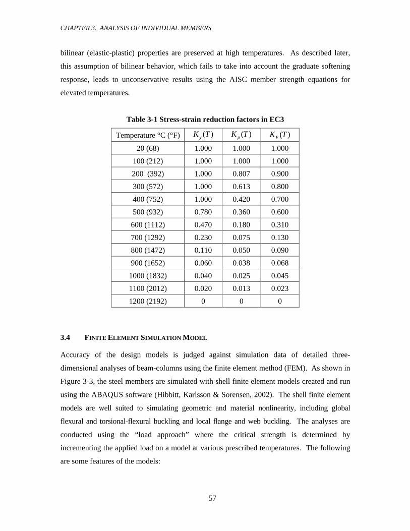
CHAPTER 3. ANALYSIS OF INDIVIDUAL MEMBERS
57
bilinear (elastic-plastic) properties are preserved at high temperatures. As described later,
this assumption of bilinear behavior, which fails to take into account the graduate softening
response, leads to unconservative results using the AISC member strength equations for
elevated temperatures.
Table 3-1 Stress-strain reduction factors in EC3
Temperature °C (°F) ( )yK T ( )pK T ( )EK T
20 (68) 1.000 1.000 1.000
100 (212) 1.000 1.000 1.000
200 (392) 1.000 0.807 0.900
300 (572) 1.000 0.613 0.800
400 (752) 1.000 0.420 0.700
500 (932) 0.780 0.360 0.600
600 (1112) 0.470 0.180 0.310
700 (1292) 0.230 0.075 0.130
800 (1472) 0.110 0.050 0.090
900 (1652) 0.060 0.038 0.068
1000 (1832) 0.040 0.025 0.045
1100 (2012) 0.020 0.013 0.023
1200 (2192) 0 0 0
3.4 FINITE ELEMENT SIMULATION MODEL
Accuracy of the design models is judged against simulation data of detailed three-
dimensional analyses of beam-columns using the finite element method (FEM). As shown in
Figure 3-3, the steel members are simulated with shell finite element models created and run
using the ABAQUS software (Hibbitt, Karlsson & Sorensen, 2002). The shell finite element
models are well suited to simulating geometric and material nonlinearity, including global
flexural and torsional-flexural buckling and local flange and web buckling. The analyses are
conducted using the “load approach” where the critical strength is determined by
incrementing the applied load on a model at various prescribed temperatures. The following
are some features of the models:

CHAPTER 3. ANALYSIS OF INDIVIDUAL MEMBERS
58
1. The member is subdivided into 32 shell elements along its length, and the flanges and
web are each subdivided into eight elements across the cross section (Figure 3-3).
Each element has eight nodes and four Gaussian integration points in the shell plane
with three point Simpson’s rule integration through the shell thickness.
2. Nonlinear stress-strain curves of steel at the elevated temperatures are adopted from
EC3, as shown in Figure 3-2(a). A uniform temperature distribution is assumed
through the member cross section and along its length. Multiaxial yielding is
modeled through the von-Mises yield criterion. The yield strengths are assumed to
be equal to their nominal specified values, so as to provide consistent comparisons
with the design models.
3. Linear kinematic constraints are applied to the flanges and web at the member end so
as to enforce planar behavior within each flange and web but to allow cross-section
warping (Figure 3-3). Displacements of the web along the Y- and Z-axis are
restrained at both ends and longitudinal displacements along the X-axis are restrained
at one end. Twisting rotation (about the X-axis) is restrained at both ends, and
rotational displacements about Y- and Z-axes (weak and strong axes) are free at both
ends.
4. For the column (axial) strength analyses, axial forces are applied along the
kinematically restrained webs and flanges at one end of the member. In one set of
analyses, the flange ends are free to rotate, thereby permitting flexural buckling about
the Y-axis (weak axis); and in a second set of analyses, rotational displacements
about the Y-axis are restrained in order to determine the flexural buckling strength
about the Z-axis (strong axis).
5. For the beam (flexural) strength analyses, a concentrated force couple is applied at
the center of upper and lower flanges at each end so as to induce a uniform strong
axis moment along the beams. The kinematic constraint across the flanges ensures a
uniform distribution of flexural stresses.
6. Initial geometric member “sweep” imperfections are modeled by introducing a single
sinusoidal curve along the member length, with a maximum initial displacement of
1/1000 of the length at the mid-span.

CHAPTER 3. ANALYSIS OF INDIVIDUAL MEMBERS
59
Figure 3-3 Shell finite element mesh and boundary conditions
0 0.002 0.004 0.006 0.008 0.010
0.2
0.4
0.6
0.8
1
δ / L
P(T
) / P
y0
20°C500°C800°C
0 0.005 0.01 0.015 0.020
0.2
0.4
0.6
0.8
1
θ (rad)
M(T
) / M
p0
20°C500°C800°C
(a) W14×90 column (L/ry=60 Gr.50) (b) W14×22 beam (L/ry = 60, Gr. 50)
Figure 3-4 Load versus displacement response from FEM simulations under ambient and elevated temperatures
Shown in Figure 3-4 are example FEM simulation results for a laterally unsupported
column and beam at ambient and elevated temperatures (20 oC, 500 oC, and 800 oC). Column
results (Figure 3-4(a)) are shown in terms of the normalized axial load versus midspan
deflection for a W14×90 column with a slenderness of / yL r = 60, where L is the length and
yr is radius of gyration about weak axis. The critical strength at 500 oC is about 50 % of that
at room temperature. This 50 % reduction is in contrast to the three material reduction factors
of yK (500 oC) = 0.78, pK (500 oC) = 0.36 and EK (500 oC) = 0.60, whose range of values
suggests that all three parameters, including the change in proportional limit, play a role in
the member strength reduction. At 800 oC the strength is about 8 % of that at room
temperature, which is in contrast to three material reduction factors of yK (800 oC) = 0.11,
pK (800 oC) = 0.05 and EK (800 oC) = 0.09. The results for 800 oC are intended as an upper

CHAPTER 3. ANALYSIS OF INDIVIDUAL MEMBERS
60
bound on the temperature response, since the large strength reduction at this temperature
suggests that the practical value of calculating the strength at this temperature is limited. The
beam data (Figure 3-4(b)) are for a W14×22 beam with a lateral slenderness of / yL r = 60
subjected to a uniformly distributed strong-axis moment. Here, the strengths reductions at
elevated temperatures are slightly less than for the column, suggesting that the beam behavior
is more dependent on the reduction in yield strength and less on the reduction in proportional
limit. In these two examples, the arc-length (Riks) solution method is used to track the post-
peak response. For the parametric studies shown later, where only the peak strength is
reported, the finite element analyses were run under load control up to the critical strength
limit state. This was done as a practical measure to reduce the analysis run times.
Analyses were also conducted to assess the effects of thermally-induced residual stresses
and cross-section imperfections on critical loads. Residual stresses were introduced with the
distribution shown in Figure 3-5(a), assuming a peak residual stress at ambient temperature
of 0rF = 69 MPa (10 ksi). Under elevated temperatures the peak residual stresses are
assumed to reduce in proportional to the reduction in yield stress, i.e., 0( ) ( )r y rF T K T F= .
Shown in Figure 3-5(b) are critical column strengths obtained from simulations run with and
without residual stresses at an elevated temperature of 500 oC. The largest difference occurs
at slenderness of about / yL r = 100, where the residual stresses reduce the critical calculated
load by less than 15 %. Residual stresses are modeled in this same way for the parametric
subsequent parametric analyses presented later.
0 50 100 150 200
0
0.2
0.4
0.6
0.8
1
L / r
Pcr
(T) /
Py(T
)
Without σr
With σr
(a) Residual stress pattern (b) Critical weak-axis buckling strength
Figure 3-5 Influence of residual stresses (W14×90 Gr. 50 column at 500 °C)

CHAPTER 3. ANALYSIS OF INDIVIDUAL MEMBERS
61
While the primary focus of this study is on compact or near-compact sections, the
significance of local flange or web buckling and local geometric imperfections was
considered. Previous research has reported that local buckling is not particularly critical at
elevated temperatures for structural sections, for which local buckling is not critical at
ambient temperature (Wang, 2002; Uy and Bradford, 1995; Ranby, 1998). This observation
is corroborated by this study where local buckling was only observed as governing the
strength limit state in a few of the FEM analyses of very short columns where the web width-
thickness ratios exceed the AISC requirements for compact column sections. To help assess
the significance of local geometric imperfections, a W14×90 (Grade 50) column of varying
slenderness was analyzed with and without local imperfections at an elevated temperature of
500 oC. The local imperfections were defined by scaling the first-mode local buckling shape,
obtained by a linear buckling analysis, to a maximum amplitude of 1/1000 of the local
buckling length (equal to a peak flange and web imperfection of about 0.5 mm). Strength
deterioration due to the local imperfection was only observed for the shorter members
(lengths of 3.1 m for flexural buckling about the strong axis and 1.9 m for flexural buckling
about the minor axis), where the maximum difference in critical strengths for analyses with
and without the imperfection are 5 % and 3 % for flexural bucking about strong and weak
axes, respectively. Thus, these analyses support the assumption that the member strengths
are no more sensitive to local buckling at elevated temperatures as compared to ambient
temperatures, and the response of compact (and near-compact) sections are fairly insensitive
to local geometric imperfections.
3.5 COLUMN STRENGTH ASSESSMENT
Many numerical and experimental studies have been carried out on the behavior of steel
columns under elevated temperatures (Burgess et al., 1992; Poh and Bennetts, 1995;
Talamona et al., 1996; Toh et al., 2000; Baker et al., 1997). Franssen et al. (1995) used finite
element techniques to numerically simulate column response under elevated temperatures
and proposed new column design equations for EC3. Talamona et al. (1997) and Franssen et
al. (1998) subsequently performed comprehensive analytical studies to investigate the critical
temperatures for various I-shaped sections with varying slenderness ratios, yield stresses,
member orientations, axial loads, and loading eccentricities. They used the critical axial
column strengths from these analyses to confirm the proposed design equations by Franssen

CHAPTER 3. ANALYSIS OF INDIVIDUAL MEMBERS
62
et al. (1995). The EC3 column design equations (EC3, 2003) have since been modified to
incorporate the proposed revisions. These prior studies provide the impetus for this current
study to independently assess the nominal strength provisions of the latest EC3 (2003)
standard and the new AISC (2005) specification.
3.5.1 AISC Column Strength Equations
The nominal column strength 0,cr AISCP of the AISC specification at ambient temperature is
calculated as follows:
For 0 02.25y eF F≤ 0
00, 00.658
y
e
FF
cr AISC yP AF⎡ ⎤⎢ ⎥=⎢ ⎥⎣ ⎦
(3.2)
For 0 02.25y eF F> 0, 00.877cr AISC eP AF= (3.3)
where 2
00 2e
EFKLr
π=
⎛ ⎞⎜ ⎟⎝ ⎠
(3.4)
where, 0yF and 0E are the yield stress and elastic modulus; 0eF is elastic buckling stress,
given by (3.4); and A , r , and K are cross-sectional area, radius of gyration, and effective
buckling length factor, respectively.
The AISC equations for calculating the critical load at elevated temperatures,
, ( )cr AISCP T , are identical to Eqs. from (3.2) to (3.4), except that the elastic modulus and yield
strength terms are replaced by their temperature dependent counterparts, ( )E T and ( )yF T ,
which are determined using the EC3 reduction factors of Eq. (3.1) and Table 3-1.
3.5.2 EC3 Column Strength Equations
The EC3 column strength 0, 3cr ECP at ambient temperature is calculated as follows:
0, 3 0 0 cr EC yP Pχ= (3.5)
0 2 2
0 0 0
1= 1.0χϕ ϕ λ
≤+ −
(3.6)
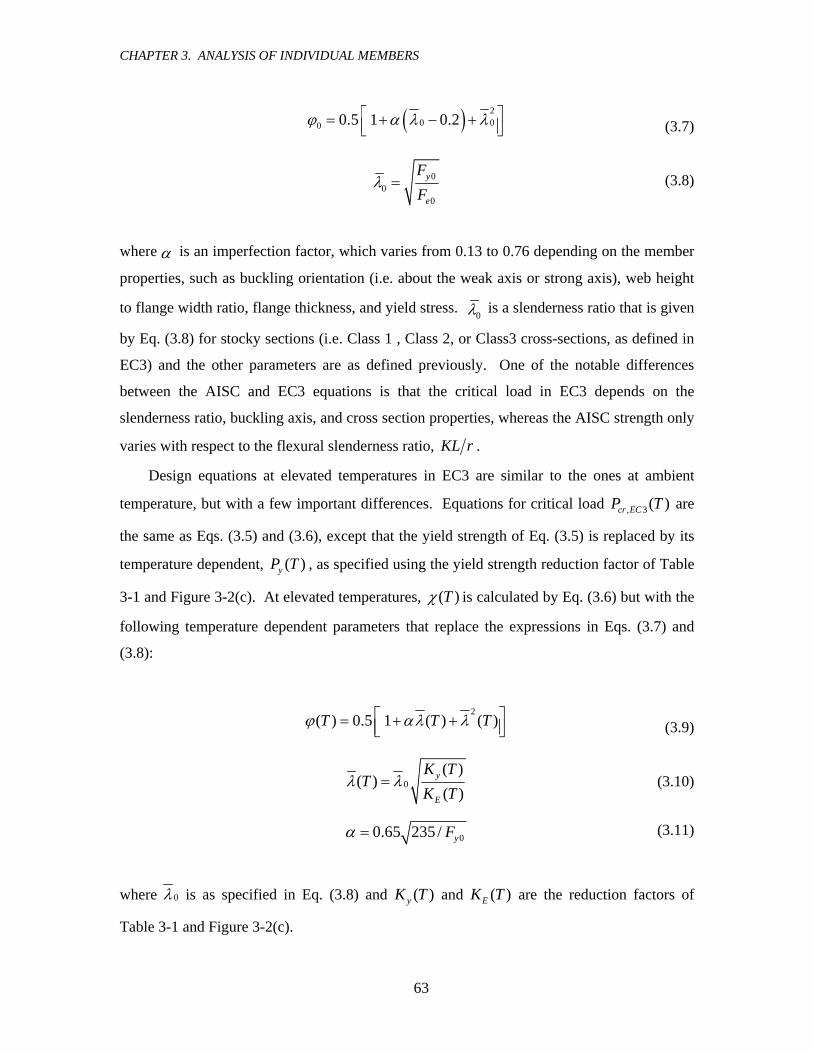
CHAPTER 3. ANALYSIS OF INDIVIDUAL MEMBERS
63
( ) 20 00 0.5 1 0.2ϕ α λ λ⎡ ⎤= + − +⎢ ⎥⎣ ⎦ (3.7)
00
0
y
e
FF
λ = (3.8)
where α is an imperfection factor, which varies from 0.13 to 0.76 depending on the member
properties, such as buckling orientation (i.e. about the weak axis or strong axis), web height
to flange width ratio, flange thickness, and yield stress. 0λ is a slenderness ratio that is given
by Eq. (3.8) for stocky sections (i.e. Class 1 , Class 2, or Class3 cross-sections, as defined in
EC3) and the other parameters are as defined previously. One of the notable differences
between the AISC and EC3 equations is that the critical load in EC3 depends on the
slenderness ratio, buckling axis, and cross section properties, whereas the AISC strength only
varies with respect to the flexural slenderness ratio, KL r .
Design equations at elevated temperatures in EC3 are similar to the ones at ambient
temperature, but with a few important differences. Equations for critical load , 3 ( )cr ECP T are
the same as Eqs. (3.5) and (3.6), except that the yield strength of Eq. (3.5) is replaced by its
temperature dependent, ( )yP T , as specified using the yield strength reduction factor of Table
3-1 and Figure 3-2(c). At elevated temperatures, )(Tχ is calculated by Eq. (3.6) but with the
following temperature dependent parameters that replace the expressions in Eqs. (3.7) and
(3.8):
2
( ) 0.5 1 ( ) ( )T T Tϕ α λ λ⎡ ⎤= + +⎢ ⎥⎣ ⎦ (3.9)
0( )
( )( )
y
E
K TT
K Tλ λ= (3.10)
00.65 235 / yFα = (3.11)
where 0λ is as specified in Eq. (3.8) and ( )yK T and ( )EK T are the reduction factors of
Table 3-1 and Figure 3-2(c).
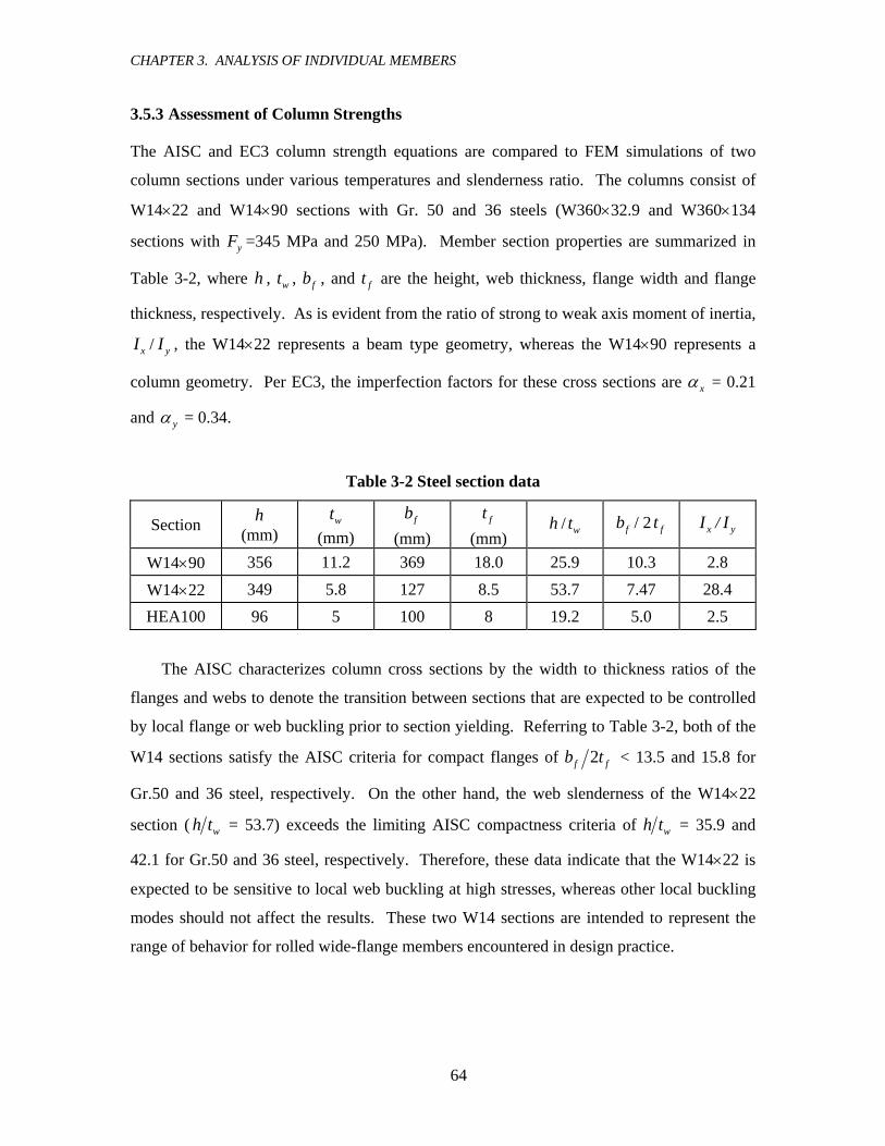
CHAPTER 3. ANALYSIS OF INDIVIDUAL MEMBERS
64
3.5.3 Assessment of Column Strengths
The AISC and EC3 column strength equations are compared to FEM simulations of two
column sections under various temperatures and slenderness ratio. The columns consist of
W14×22 and W14×90 sections with Gr. 50 and 36 steels (W360×32.9 and W360×134
sections with yF =345 MPa and 250 MPa). Member section properties are summarized in
Table 3-2, where h , wt , fb , and ft are the height, web thickness, flange width and flange
thickness, respectively. As is evident from the ratio of strong to weak axis moment of inertia,
xI / yI , the W14×22 represents a beam type geometry, whereas the W14×90 represents a
column geometry. Per EC3, the imperfection factors for these cross sections are xα = 0.21
and yα = 0.34.
Table 3-2 Steel section data
Section h (mm)
wt (mm)
fb (mm)
ft (mm)
h / wt fb / 2 ft xI / yI
W14×90 356 11.2 369 18.0 25.9 10.3 2.8
W14×22 349 5.8 127 8.5 53.7 7.47 28.4 HEA100 96 5 100 8 19.2 5.0 2.5
The AISC characterizes column cross sections by the width to thickness ratios of the
flanges and webs to denote the transition between sections that are expected to be controlled
by local flange or web buckling prior to section yielding. Referring to Table 3-2, both of the
W14 sections satisfy the AISC criteria for compact flanges of 2f fb t < 13.5 and 15.8 for
Gr.50 and 36 steel, respectively. On the other hand, the web slenderness of the W14×22
section ( wh t = 53.7) exceeds the limiting AISC compactness criteria of wh t = 35.9 and
42.1 for Gr.50 and 36 steel, respectively. Therefore, these data indicate that the W14×22 is
expected to be sensitive to local web buckling at high stresses, whereas other local buckling
modes should not affect the results. These two W14 sections are intended to represent the
range of behavior for rolled wide-flange members encountered in design practice.

CHAPTER 3. ANALYSIS OF INDIVIDUAL MEMBERS
65
0 50 100 150 2000
0.2
0.4
0.6
0.8
1
L / r
Pcr
0 / P
y0
ABAQUS-SABAQUS-WAISCEC3-SEC3-W
0 50 100 150 2000
0.2
0.4
0.6
0.8
1
L / r
Pcr
(T) /
Py(T
)
ABAQUS-SABAQUS-WAISCEC3Proposed
(a) ambient temperature (b) 100 °C
0 50 100 150 2000
0.2
0.4
0.6
0.8
1
L / r
Pcr
(T) /
Py(T
)
ABAQUS-SABAQUS-WAISCEC3Proposed
0 50 100 150 2000
0.2
0.4
0.6
0.8
1
L / r
Pcr
(T) /
Py(T
)
ABAQUS-SABAQUS-WAISCEC3Proposed
(c) 200 °C (d) 300 °C
0 50 100 150 2000
0.2
0.4
0.6
0.8
1
L / r
Pcr
(T) /
Py(T
)
ABAQUS-SABAQUS-WAISCEC3Proposed
0 50 100 150 2000
0.2
0.4
0.6
0.8
1
L / r
Pcr
(T) /
Py(T
)
ABAQUS-SABAQUS-WAISCEC3Proposed
(e) 400 °C (f) 500 °C

CHAPTER 3. ANALYSIS OF INDIVIDUAL MEMBERS
66
0 50 100 150 2000
0.2
0.4
0.6
0.8
1
L / r
Pcr
(T) /
Py(T
)
ABAQUS-SABAQUS-WAISCEC3Proposed
0 50 100 150 2000
0.2
0.4
0.6
0.8
1
L / r
Pcr
(T) /
Py(T
)
ABAQUS-SABAQUS-WAISCEC3Proposed
(g) 600 °C (h) 700 °C
0 50 100 150 2000
0.2
0.4
0.6
0.8
1
L / r
Pcr
(T) /
Py(T
)
ABAQUS-SABAQUS-WAISCEC3Proposed
(i) 800 °C
Figure 3-6 Critical compressive strengths of W14×90 Gr.50 column
Superimposed in Figure 3-6(a) are FEM simulation results and nominal strengths
calculated according to the AISC and EC3 provisions for the W14×90 (Gr. 50) column at
ambient temperature. These results are shown as a benchmark against which to judge the
differences in the models at elevated temperatures. Critical strengths of member were
investigated for elevated temperature increments of 100 °C up to 800 °C. Representative
results are shown in Figure 3-6(b)-(i) for temperatures from 200 °C to 800 °C. As noted
previously, the results at 800 °C have limited practical impact but are included to show the
bounds of response. Simulation results are shown for both strong and weak axis buckling for
slenderness ratios between from 20 to 200. Compared to the ambient temperature case, the
differences between simulated results for strong versus weak axes decrease at higher
temperatures. Clearly evident in these figures is that the AISC strength equations are

CHAPTER 3. ANALYSIS OF INDIVIDUAL MEMBERS
67
unconservative at elevated temperatures, particularly for slenderness ratios between 40 and
100 and temperatures above 500 °C. For instance, referring to the strength ratio comparisons
in Figure 3-7, at 500 °C the nominal strengths calculated by the AISC provisions are up to 60
% larger than the critical strengths as calculated by simulation. On the other hand, the EC3
column strength equations match the simulated results within about 20 %.
0 50 100 150 200
-20
0
20
40
60
L / r
Erro
r (%
)AISCEC3Proposed
Figure 3-7 Percentage error in the calculated compression strength of W14×90
Gr.50 column at 500 °C
3.5.4 Proposed Column Strength Equations
Motivated by the large discrepancy between the AISC provisions and the simulated results,
the authors developed an alternative column strength equation that is similar in format to the
AISC equations but with greatly improved accuracy at high temperatures. The proposal is to
use the following equation for elevated temperatures in lieu of Eqs. (3.2) and (3.3):
( )( )
, ( ) 0.42 ( )y
e
F TF T
cr Prop yP T AF T⎡ ⎤⎢ ⎥=⎢ ⎥⎣ ⎦
(3.12)
where 2
2( )( )e
E TF TKLr
π=
⎛ ⎞⎜ ⎟⎝ ⎠
(3.13)
This equation is similar to the AISC equation (2) but with a different coefficient and
exponent. Like the AISC equations, this model utilizes the EC3 reduction factors to calculate
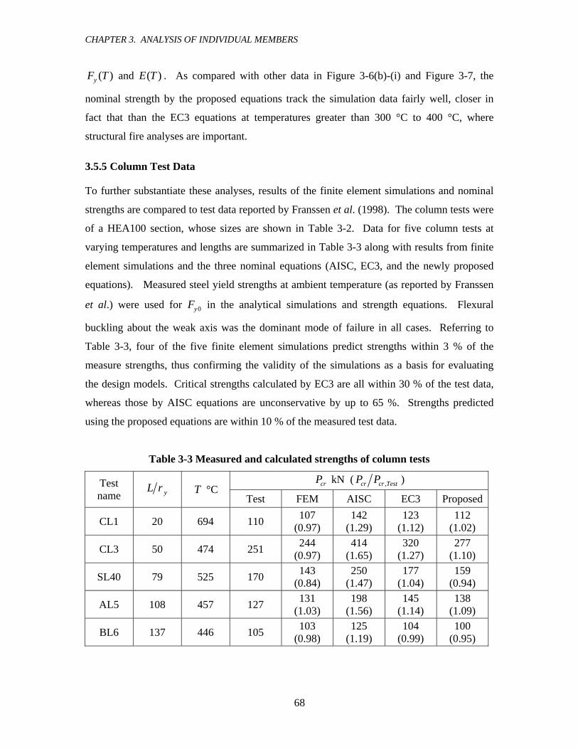
CHAPTER 3. ANALYSIS OF INDIVIDUAL MEMBERS
68
( )yF T and ( )E T . As compared with other data in Figure 3-6(b)-(i) and Figure 3-7, the
nominal strength by the proposed equations track the simulation data fairly well, closer in
fact that than the EC3 equations at temperatures greater than 300 °C to 400 °C, where
structural fire analyses are important.
3.5.5 Column Test Data
To further substantiate these analyses, results of the finite element simulations and nominal
strengths are compared to test data reported by Franssen et al. (1998). The column tests were
of a HEA100 section, whose sizes are shown in Table 3-2. Data for five column tests at
varying temperatures and lengths are summarized in Table 3-3 along with results from finite
element simulations and the three nominal equations (AISC, EC3, and the newly proposed
equations). Measured steel yield strengths at ambient temperature (as reported by Franssen
et al.) were used for 0yF in the analytical simulations and strength equations. Flexural
buckling about the weak axis was the dominant mode of failure in all cases. Referring to
Table 3-3, four of the five finite element simulations predict strengths within 3 % of the
measure strengths, thus confirming the validity of the simulations as a basis for evaluating
the design models. Critical strengths calculated by EC3 are all within 30 % of the test data,
whereas those by AISC equations are unconservative by up to 65 %. Strengths predicted
using the proposed equations are within 10 % of the measured test data.
Table 3-3 Measured and calculated strengths of column tests
crP kN ( ,cr cr TestP P ) Test name yL r T °C
Test FEM AISC EC3 Proposed
CL1 20 694 110 107 (0.97)
142 (1.29)
123 (1.12)
112 (1.02)
CL3 50 474 251 244 (0.97)
414 (1.65)
320 (1.27)
277 (1.10)
SL40 79 525 170 143 (0.84)
250 (1.47)
177 (1.04)
159 (0.94)
AL5 108 457 127 131 (1.03)
198 (1.56)
145 (1.14)
138 (1.09)
BL6 137 446 105 103 (0.98)
125 (1.19)
104 (0.99)
100 (0.95)

CHAPTER 3. ANALYSIS OF INDIVIDUAL MEMBERS
69
3.5.6 Influence of Yield Strength and Section Geometry
Results of analyses to examine the influence of yield strength and section properties are
shown in Figure 3-8(a)-(b). Comparing Figure 3-8(a) to Figure 3-6(f), the trends in both the
simulation and relative accuracy of the design equations is essentially the same for Gr. 36 as
Gr. 50 steel. The influence of section proportions (W14×22 versus W14×90) is seen by
comparing Figure 3-8(b) and Figure 3-6(f). For the W14×22 only minor axis flexural
buckling is considered due to the large difference in strong versus weak axis properties. In
Figure 3-8(b) the effect of web slenderness web in the W14×22 is apparent, where the
simulated results drop off compared to the design equations at low slenderness ( /L r < 30)
where the critical stress exceeds about 0.6 ( )yF T . This occurs because at these stress levels
local web buckling, which is not reflected in the column strength equations, begins to control
the critical strength. It turns out that for this column, these discrepancies are not of much
practical significance since the column length corresponding to /L r = 30 is only 0.80 m.
Except for these cases where web buckling is critical (and is expected based on the fact that
the / wh t exceeds the AISC limit for compact webs), the critical strengths agree well with the
proposed equation. Additional analyses of the W14×22 section at other temperatures confirm
that the critical web buckling stress of about 0.6 ( )yF T is fairly constant across various
temperature ranges.
0 50 100 150 2000
0.2
0.4
0.6
0.8
1
L / r
Pcr
(T) /
Py(T
)
ABAQUS-SABAQUS-WAISCEC3Proposed
(a) W14×90 Gr.36
0 50 100 150 2000
0.2
0.4
0.6
0.8
1
L / r
Pcr
(T) /
Py(T
)
ABAQUS-WAISCEC3Proposed
(b) W14×22 Gr.50
Figure 3-8 Comparative assessment of column compression strength at 500 °C
CHAPTER 3. ANALYSIS OF INDIVIDUAL MEMBERS
70
3.6 BEAM STRENGTH ASSESSMENT
Design equations for laterally unsupported beams require evaluation of torsional-flexural
instability effects, which for I-shaped sections involves consideration of non-uniform torsion
and warping restraint. Compared to columns and laterally supported beams, there are
relatively few studies of laterally unsupported beams under fire conditions. Bailey et al.
(1996) studied the critical temperatures for several beam sections with different loading
patterns and commented that the then current EC3 provisions were unconservative for
laterally unsupported beams. Piloto and Vila Real (2000) performed an experimental study
of electronically heated beams and reported that the measured critical temperatures were
scattered and generally higher than the theoretical or design temperatures. They attributed
the variations to the complexity of the phenomena and the difficulty in conducting the
experiments. Vila Real et al. (2000, 2004a, 2004b) numerically studied the critical
temperatures and strength for various loading patterns, from which they proposed alternative
design equations that were later incorporated in EC3 (2003).
Building upon prior research, analytical results for laterally unsupported beams are
compared with design equations of the AISC and EC3 specifications, similar to the column
comparisons. As in the column study, the large discrepancy between the AISC strength
equations and simulation results prompted the proposal of alternative equations for
evaluating beams at elevated temperatures.
3.6.1 AISC Beam Strength Equations
The AISC equations for beam strength at ambient temperature are given by the following
equations, where 0pM is the plastic moment and 0rM is the initial yield moment (reduced to
account for residual stresses), 0E and 0G are the elastic moduli, J is the torsional constant,
wC is the warping constant, and λ is the slenderness ratio (= / yL r ):
For 0pλ λ≤ 0, 0cr AISC pM M= (3.14)
For 0 0p rλ λ λ< ≤ ( ) 00, 0 0 0
0 0
pcr AISC p p r
r p
M M M Mλ λ
λ λ⎛ ⎞−
= − − ⎜ ⎟⎜ ⎟−⎝ ⎠ (3.15)
CHAPTER 3. ANALYSIS OF INDIVIDUAL MEMBERS
71
For 0rλ λ> 2
00, 0 0cr AISC y y w
y y
EM E I G J I Cr r
ππλ λ
⎛ ⎞= + ⎜ ⎟⎜ ⎟
⎝ ⎠ (3.16)
The slenderness ratios, 0pλ and 0rλ , correspond to the transitions between full plastic
bending capacity, inelastic lateral-torsional buckling, and elastic lateral-torsional buckling,
represented by Eqs. (3.14), (3.15) and (3.16), respectively. 0pλ is determined from empirical
data, while 0rλ corresponds to the theoretical slenderness where the critical elastic buckling
moment, per Eq. (3.16), is equal to the initial yield moment 0rM . The critical moment for
elastic lateral torsional buckling with Eq. (3.16) is theoretically derived (Timoshenko and
Gere, 1961) and that for inelastic buckling with Eq. (3.15) is a linear interpolation between
the transition points with Eqs. (3.14) and (3.16). These transition points are calculated by the
following equations, where xS is the elastic section modulus about strong axis and the other
terms are as defined previously:
00
0
1.76py
EF
λ = (3.17)
2100 2 0
0
1 1r LL
X X FF
λ = + + (3.18)
0 0r x LM S F= (3.19)
where 0 010 2x
E G JAXSπ
= (3.20)
2
2 4 w x
y
C SXI GJ
⎛ ⎞= ⎜ ⎟⎝ ⎠
(3.21)
0 00.7L yF F= (3.22)
As specified in AISC (2005), the critical moment under elevated temperatures
, ( )cr AISCM T is obtained from Eqs. (3.14) to (3.21) by modifying E, G and yF using the
reduction coefficients ( )EK T and ( )yK T .

CHAPTER 3. ANALYSIS OF INDIVIDUAL MEMBERS
72
3.6.2 EC3 Beam Strength Equations
The EC3 beam strength equations at ambient temperature have a similar format to the EC3
column equations:
0, 3 0 0 cr EC LT pM Mχ= (3.23)
0 2 20 0 0
1 = 1.0LT
LT LT LT
χϕ ϕ λ
≤+ −
(3.24)
where
2
0 00 0.5 1 ( 0.2)LT LTLT LTϕ α λ λ⎡ ⎤= + − +⎢ ⎥⎣ ⎦ (3.25)
00
0,
pLT
cr e
MM
λ = (3.26)
0 0p x yM Z F= (3.27)
and 0LTχ is the reduction factor for lateral torsional buckling, LTα is an imperfection
factor which depends on the section proportions ( LTα = 0.21 is used for rolled sections with
the web height to flange width ratio / 2fh b ≤ and LTα = 0.34 for / 2fh b > ), 0,cr eM is the
elastic critical moment for lateral torsional buckling, and xZ is plastic modulus about strong
axis. Eq. (3.26) is specified for compact sections, which correspond to the Class 1 or Class 2
designations in EC3.
Differences between the beam equations in EC3 under fire conditions and at ambient
temperature are similar to those between the corresponding column equations. The primary
changes are in the definition of LTϕ , LTα , and LTλ , which are defined for elevated
temperatures by the following equations that replace Eqs. (3.25) - (3.27):
2 ( )=0.5[1+ ( ) ( )]LT LT LT LTT T Tϕ α λ λ+ (3.28)
0=0.65 235/LT yFα (3.29)
0
( )( )
( )y
LT LTE
K TT
K Tλ λ= (3.30)

CHAPTER 3. ANALYSIS OF INDIVIDUAL MEMBERS
73
Note that 0yF carries units of MPa in Eq. (3.29).
3.6.3 Proposed Beam Strength Equations
As an alternative to the AISC beam strength equations, the following equations are proposed
to evaluate bending strengths at elevated temperatures using a similar format to the AISC
design equations:
For ( )r Tλ λ≤ ( )
, ( ) ( ) ( ) ( ) 1( )
XC T
cr Prop r p rr
M T M T M T M TT
λλ
⎛ ⎞⎡ ⎤= + − −⎜ ⎟⎣ ⎦
⎝ ⎠ (3.31)
For ( )r Tλ λ> 2
,( )( ) ( ) ( )cr Prop y y w
y y
E TM T E T I G T J I Cr r
π πλ λ
⎛ ⎞= + ⎜ ⎟⎜ ⎟
⎝ ⎠ (3.32)
In contrast to the equations at ambient temperature where the design equations are
distinguished into three regions of behavior, here only two equations are used to model
inelastic and elastic lateral-torsional buckling. As will be shown later, these equations reflect
that fact that at elevated temperatures the critical moment drops off quickly from the plastic
moment at small slenderness values. The distinction between inelastic and elastic behavior is
indicated by the slenderness value ( )r Tλ , which corresponds to the elastic moment at the
onset of yielding, ( )rM T . The governing equations for ( )r Tλ and ( )rM T are the same as
the AISC values, Eqs. (3.18) to (3.22) with reduced yield stress and elastic modulus, except
that the initial yield stress LF is replaced by the following:
( ) ( ) ( )L p rF T F T F T= − (3.33)
0( ) ( )p p yF T K T F= (3.34)
0( ) ( )r y rF T K T F= (3.35)
Compared to the original AISC equations, the major change is to base ( )LF T on the
temperature dependent proportional limit ( )pF T rather than the yield stress. 0rF is the
residual stress at the ambient temperature, which is specified in AISC as 0rF = 69 MPa for

CHAPTER 3. ANALYSIS OF INDIVIDUAL MEMBERS
74
rolled shapes. Implied in Eq. (3.35) is the assumption that the residual stresses under elevated
temperatures are proportional to the reduction factor of yield strength, ( )yK T . The
term ( )XC T in Eq. (3.31) is an exponent that is defined as a bilinear function with respect to
the temperature according to the following equation for T > 100 oC,
( ) 0.6250XTC T = +
≤ 3.0 (3.36)
where T carries units of oC.
3.6.4 Assessment of Beam Strengths
Comparisons between the simulated results and design equations for bending strength are
shown in Figure 3-9 through Figure 3-11. Simulated results for a W14×22 Gr. 50 ( yF =345
MPa) beam of varying lateral slenderness are compared to the AISC and EC3 equations at
ambient temperatures in Figure 3-9(a). As in the column analyses, the simulated points
correspond to the peak point in load versus deflection curves, such as shown previously in
Figure 3-4(b). The comparison in Figure 3-9(a) demonstrates that even at ambient
temperatures, the AISC flexure equations tend to be unconservative relative to the simulated
results and EC3 equations. In this example, the maximum error occurs at an intermediate
slenderness, λ = 100, where the AISC strength is about 30 % larger than the simulated
results.

CHAPTER 3. ANALYSIS OF INDIVIDUAL MEMBERS
75
0 50 100 150 2000
0.2
0.4
0.6
0.8
1
λ = Lb / ry
Mcr
0 / M
p0
ABAQUSAISCEC3
0 50 100 150 2000
0.2
0.4
0.6
0.8
1
λ = Lb / ry
Mcr
(T) /
Mp(T
)
ABAQUSAISCEC3Proposed
(a) ambient temperature (b) 100 °C
0 50 100 150 2000
0.2
0.4
0.6
0.8
1
λ = Lb / ry
Mcr
(T) /
Mp(T
)
ABAQUSAISCEC3Proposed
0 50 100 150 2000
0.2
0.4
0.6
0.8
1
λ = Lb / ry
Mcr
(T) /
Mp(T
)
ABAQUSAISCEC3Proposed
(c) 200 °C (d) 300 °C
0 50 100 150 2000
0.2
0.4
0.6
0.8
1
λ = Lb / ry
Mcr
(T) /
Mp(T
)
ABAQUSAISCEC3Proposed
0 50 100 150 2000
0.2
0.4
0.6
0.8
1
λ = Lb / ry
Mcr
(T) /
Mp(T
)
ABAQUSAISCEC3Proposed
(e) 400 °C (f) 500 °C

CHAPTER 3. ANALYSIS OF INDIVIDUAL MEMBERS
76
0 50 100 150 2000
0.2
0.4
0.6
0.8
1
λ = Lb / ry
Mcr
(T) /
Mp(T
)
ABAQUSAISCEC3Proposed
0 50 100 150 2000
0.2
0.4
0.6
0.8
1
λ = Lb / ry
Mcr
(T) /
Mp(T
)
ABAQUSAISCEC3Proposed
(g) 600 °C (h) 700 °C
0 50 100 150 2000
0.2
0.4
0.6
0.8
1
λ = Lb / ry
Mcr
(T) /
Mp(T
)
ABAQUSAISCEC3Proposed
(i) 800 °C
Figure 3-9 Critical bending moment strengths of W14×22 Gr.50 beam
0 50 100 150 200-20
0
20
40
60
80
100
L / r
Erro
r (%
)
AISCEC3Proposed
Figure 3-10 Percentage error in the calculated bending moment strength of
W14×22 Gr.50 beam at 500 °C

CHAPTER 3. ANALYSIS OF INDIVIDUAL MEMBERS
77
0 50 100 150 2000
0.2
0.4
0.6
0.8
1
λ = Lb / ry
Mcr
(T) /
Mp(T
)
W14x22 Fy 250MPa T 500 C
ABAQUSAISCEC3Proposed
(a) W14×22 Gr.36
0 50 100 150 2000
0.2
0.4
0.6
0.8
1
λ = Lb / ry
Mcr
(T) /
Mp(T
)
W14x90 Fy 345MPa T 500 C
ABAQUSAISCEC3Proposed
(b) W14×90 Gr.50
Figure 3-11 Comparative assessment of beam bending moment strength at 500 °C
Strengths for the W14×22 beam at elevated temperatures, 200 °C, 500 °C and 800 °C,
are compared in Figure 3-9(b)-(i). Included are the FEM simulation results and the nominal
strengths calculated by the three design equations (AISC, EC3, and the proposed model).
Immediately apparent from these comparisons are the large discrepancies between the AISC
equations and the simulated results. Referring to Figure 3-10, at 500 °C the largest
percentage differences occur for intermediate slenderness values of λ = 80 to 100, where the
AISC strengths are about 80% higher than the simulated strengths at temperatures. In part,
the discrepancies arise because at elevated temperatures the simulated results indicate that the
moment strength drops off quickly with increasing slenderness, whereas the AISC equations
preserve the plastic moment, ( )pM T , up to about λ = 40. In contrast to the AISC equations,
the EC3 model tracks the simulated results fairly well.
As indicated previously, the new equations proposed by the authors are intended to
provide good accuracy while maintaining a similar concept and format of the AISC
equations. One of the basic features of the proposed model is that it preserves use of the
elastic critical load at high slenderness values. At lower temperatures (e.g., 200 °C) the
transition between the inelastic and elastic response, at λ = 110, is quite abrupt. At higher
temperature, as the proportional limit is reduced through ( )pK T , the inelastic curve controls
over a larger range of slenderness. As evident from Figure 3-9(e)-(i) and Figure 3-10, at
above about 400 °C results from the proposed model and the EC3 model are quite similar and
agree well with the simulation data. The proposed model is less conservative than the EC3

CHAPTER 3. ANALYSIS OF INDIVIDUAL MEMBERS
78
equations at lower temperatures (e.g., 200 °C in Figure 3-9(b)-(d)), owing to the desire to
maintain close conformance with the AISC relationships at ambient temperature.
Results shown in Figure 3-11 illustrate that the trends observed in Figure 3-9 for the
W14×22 Gr. 50 beam are generally representative of other yield strengths and section
properties. Results for Gr. 36 steel ( yF = 250 MPa) at 500 °C are shown in Figure 3-11(a).
Here the effect of the residual stresses (assumed at 0rF = 69 MPa at ambient temperature) are
proportionally larger for the Gr. 36 steel, and the increased softening effect leads to closer
agreement between the EC3 and proposed equations, as compared to the results shown in
Figure 3-9(f) for Gr. 50 steel. Results for a W14×90 Gr. 50 beam at 500 °C are shown in
Figure 3-11(b). In this case, the strengths calculated by the EC3 and proposed models agree
very well with the simulated results up to about λ = 100. At higher slenderness these two
models tend to underestimate the critical load, because the proportions of the W14×90
(smaller xI / yI ratio) are such that the in-plane pre-buckling deformations tend to increase
the critical load. This beneficial effect of in-plane deflections is picked up in the simulation
but not in the critical load equations. Overall, the results in Figure 3-11 confirm that the EC3
and the proposed models provide accurate results for the typical range of steel shapes and
yield strengths used in practice.
3.7 BEAM-COLUMN STRENGTH ASSESSMENT
Laterally unsupported beam-columns subjected to combined axial compression and strong
axis bending experience combined limit states of yielding, lateral buckling and lateral
torsional buckling. As with laterally unsupported beams, there are relatively few studies of
design equations for beam-columns under fire conditions. Lopes et al. (2004) compared
numerical simulations to equations in the 1995 and 2003 editions of EC3 and confirmed that
the 2003 provisions are more accurate and conservative than the 1995 provisions. Toh et al.
(2000) proposed an approach to find combinations of the critical axial force and bending moment
using Rankin’s method. In the following discussion, results of the present study of columns and
beams is extended to evaluate the AISC and EC3 design equations for beam-columns subjected
to axial load and major-axis bending.

CHAPTER 3. ANALYSIS OF INDIVIDUAL MEMBERS
79
3.7.1 AISC Beam-Column Strength Equations
The AISC beam-column strength equations employ a simple bilinear combination of the ratio
of axial and bending effects. As given by the following, the equations for elevated
temperatures are identical to those at ambient temperatures except that the nominal strengths
are calculated at elevated temperatures:
For ,
0.2( )
u
cry AISC
PP T
≥ , ,
8 1.0( ) 9 ( )
u ux
cry AISC crx AISC
P MP T M T
+ ≤ (3.37)
For ,
0.2( )
u
cry AISC
PP T
< , ,
1.02 ( ) ( )
u ux
cry AISC crx AISC
P MP T M T
+ ≤ (3.38)
where uP and uxM are the factored axial load and bending moment about the strong axis
and , ( )cry AISCP T and , ( )crx AISCM T are the critical axial strength for flexural buckling and the
critical bending moment for lateral torsional buckling, respectively. Assuming the member
to be pin-ended about both axes, the column strength , ( )cry AISCP T is controlled by flexural
buckling about the weak axis. Per the AISC Specification, uxM should include second-order
effects. For the pin-ended column subjected to uniform end moments, ,x endM , the second-
order moment at the mid-span is calculate as:
,
,
( )1 ( )
x endux
u cr e
MM T
P P T=
− (3.39)
where
2
, 2
( )( )cr eE T AP T πλ
= (3.40)
According to Eq. (3.39), the second-order amplification factor is calculated based on the
critical load determined using ( )E T and per Eq. (3.1).
CHAPTER 3. ANALYSIS OF INDIVIDUAL MEMBERS
80
3.7.2 Proposed Beam-Column Strength Equations
The proposed equations employ the same interaction check and amplification factor as the
AISC equations, except that the nominal strength terms, ( )cry,PropP T and ( )cry,PropM T , are
calculated according to the newly proposed equations.
3.7.3 EC3 Beam-Column Strength Equations
The EC3 beam-column equations for combined axial load and bending moment are as
follows:
, 3 , 3
( ) ( ) 1.0( ) ( )
u uxLT
cry EC cr EC
P M Tk TP T M T
+ ≤ (3.41)
where,
, 3 ( ) ( ) ( )cry EC y yP T T P Tχ= (3.42)
, 3
( ) 1 ( )( )
uLT LT
cry EC
Pk T TP T
μ= − (3.43)
( ) 0.165 ( ) 0.15 0.9LT yT Tμ λ= − ≤ (3.44)
where uP and ( )uxM T are the factored axial load and bending moment about the strong axis
and , 3 ( )cr ECP T and , 3 ( )cr ECM T are the critical axial strength for flexural buckling and the
critical bending moment for lateral torsional buckling, respectively, and other terms are as
defined previously. Note that the Eq. (3.44) for ( )LT Tμ is shown in simplified format for a
pin-ended beam-column subjected to uniform end moments.
3.7.4 Assessment of Beam-Column Strengths
The same FEM analysis model used for the column and beam studies is used for beam-
column study, including non-uniform torsion and warping restraint effects. The limit state
combinations of axial load versus end moment are compared in Figure 3-12 for a W14×90
(Gr.50) member with λ = 60 at various elevated temperatures. The curve in the AISC and
proposed equations is due to the second-order effects in ( )uxM T per Eq. (3.39). In general
both the EC3 and proposed equations show good agreement with the simulated results. It is

CHAPTER 3. ANALYSIS OF INDIVIDUAL MEMBERS
81
difficult to say whether the bi-linear or linear interaction equations are more appropriate,
since much of the accuracy of the interaction check depends on the accuracy of the nominal
axial load and moment strength. Following the previous discussion of the axial load and
moment strengths, the AISC provisions at elevated temperatures are highly unconservative
relative to the simulated results and other design equations. The errors are larger for bending
dominated (as opposed to axial dominated) members, owing to the underlying errors in the
, ( )cr AISCM T equations discussed previously.
0 0.2 0.4 0.6 0.8 10
0.2
0.4
0.6
0.8
1
Mx,end(T) / Mp(T)
Pu(T
) / P
y(T)
ABAQUSAISCEC3Proposed
0 0.2 0.4 0.6 0.8 10
0.2
0.4
0.6
0.8
1
Mx,end(T) / Mp(T)
Pu(T
) / P
y(T)
ABAQUSAISCEC3Proposed
(a) 200 °C (b) 300 °C
0 0.2 0.4 0.6 0.8 10
0.2
0.4
0.6
0.8
1
Mx,end(T) / Mp(T)
Pu(T
) / P
y(T)
ABAQUSAISCEC3Proposed
0 0.2 0.4 0.6 0.8 10
0.2
0.4
0.6
0.8
1
Mx,end(T) / Mp(T)
Pu(T
) / P
y(T)
ABAQUSAISCEC3Proposed
(c) 400 °C (d) 500 °C

CHAPTER 3. ANALYSIS OF INDIVIDUAL MEMBERS
82
Figure 3-12 Critical axial load and moment strengths of W14×90 Gr.50 (λ=60) beam-column
Results in Figure 3-13 illustrate similar results for a lower yield steel strength and
alternative steel section. Comparing Figure 3-12(d) and Figure 3-13(a), the differences
between Gr. 50 and Gr. 36 steel at 500 °C indicate that results from the simulation, EC3 and
proposed equations tend to converge for Gr. 36 steel, presumably because the residual
stresses and non-proportional limit are closer together. Conversely, the AISC results, which
do not take into account the reduced proportional limit loose accuracy for Gr. 36. Comparing
Figure 3-12(d) and Figure 3-13(b), the differences between the W14×90 to W14×22 sections
lead to minor changes that can be traced back to differences in the axial load and moment
strengths.
0 0.2 0.4 0.6 0.8 10
0.2
0.4
0.6
0.8
1
Mx,end(T) / Mp(T)
Pu(T
) / P
y(T)
ABAQUSAISCEC3Proposed
0 0.2 0.4 0.6 0.8 10
0.2
0.4
0.6
0.8
1
Mx,end(T) / Mp(T)
Pu(T
) / P
y(T)
ABAQUSAISCEC3Proposed
(e) 600 °C (f) 700 °C
0 0.2 0.4 0.6 0.8 10
0.2
0.4
0.6
0.8
1
Mx,end(T) / Mp(T)
Pu(T
) / P
y(T)
ABAQUSAISCEC3Proposed
(g) 800 °C

CHAPTER 3. ANALYSIS OF INDIVIDUAL MEMBERS
83
0 0.2 0.4 0.6 0.8 10
0.2
0.4
0.6
0.8
1
Mx,end(T) / Mp(T)
Pu(T
) / P
y(T)
ABAQUSAISCEC3Proposed
(a) W14×90 Gr.36
0 0.2 0.4 0.6 0.8 10
0.2
0.4
0.6
0.8
1
Mx,end(T) / Mp(T)
Pu(T
) / P
y(T)
ABAQUSAISCEC3Proposed
(b) W14×22 Gr.50
Figure 3-13 Comparative assessment of beam-column strengths at 500 °C
3.8 SUMMARY AND CONCLUSIONS
Codified design equations for steel members subjected to high temperatures are an important
step towards facilitating consensus standards to evaluate the structural safety of buildings to
fire. Incorporation of fire provisions in structural design standards also raises awareness of
the issues and has encouraged research and development to validate and improve the
provisions. Design equations first introduced in the Eurocode EC3 standard in 1992 were
subsequently updated and improved through studies by a number of researchers. Similar
design requirements have only recently been introduced in a new appendix to the 2005 AISC
Specification.
The results summarized herein provide an independent assessment of the EC3 and AISC
provisions for columns, laterally unbraced beams, and laterally unbraced beam-columns,
which are compared to data from detailed nonlinear finite element analyses. Utilizing three-
dimensional shell finite elements, the numerical simulations incorporate the effects of local
and overall buckling and instability, including non-uniform torsion and warping restraint
effects. The simulation results are not entirely independent of the design standards, since the
simulation models are based on stress-strain data at elevated temperatures that is specified in
EC3 and referenced in AISC. However, through comparisons between the EC3 stress-strain
models and test data of steel at elevated temperatures and column tests, the authors have
reaffirmed the accuracy of the EC3 stress strain data. The simulation study included about

CHAPTER 3. ANALYSIS OF INDIVIDUAL MEMBERS
84
four hundred finite element analyses, including the effects of varying slenderness, steel
temperature, steel yield strength, residual stresses, and section properties.
Comparison between the AISC provisions and the simulation results indicate that the
AISC provisions significantly over-estimate the nominal strength of columns, beams and
beam-columns at elevated temperatures. The AISC column strengths were up to 60 % higher
than the simulated results, and the beam and beam-column strengths were 80-100 % higher.
These large discrepancies indicate that the approach used in the AISC provisions of simply
modifying the elastic moduli ( E and G ) and yield strength ( yF ) in the otherwise standard
(ambient temperature) design equations is inaccurate. Thus, the large variations are due
primarily to the fact that the steel stress-strain curve loses its characteristic bi-linear elastic-
plastic response at elevated temperatures. Comparisons between the EC3 provisions and
simulation results indicate that the EC3 equations are within 20 % of the simulations. This
good agreement reflects refinements made to the EC3 provisions since their first publication.
While it would be tempting to simply recommend that the EC3 provisions be adopted
into the AISC Specification, the format of the EC3 provisions is quite different from the
AISC ambient strength design provisions. In the interest of maintaining similarity in format
and style between ambient and elevated temperature provisions in the AISC Specification,
new design equations are proposed as alternatives to those in the 2005 edition of the AISC
specification. The proposed alternative equations for calculating the nominal column and
beam strengths are validated against the simulation data and reduce the discrepancies to less
than about 20-30 %, which is similar the accuracy of the EC3 provisions. While similar in
format, the proposed equations are distinct from the AISC provisions for ambient
temperatures, and thus there is a discontinuity in response between the two sets of equations.
The proposed equations are only intended for use at elevated temperatures, which can be
assumed as temperatures higher than 200 °C, a temperature that would rarely if ever be
exceeded except under fire conditions.
3.9 LIMITATIONS AND FUTURE RESEARCH
While this study helps to both validate and improve current design provisions for steel
members at elevated temperatures, the scope is limited to assessment of individual members
comprised of bi-symmetric I-shaped members with compact (or near-compact) sections. The
current study treats the problem deterministically, using nominal properties (material

CHAPTER 3. ANALYSIS OF INDIVIDUAL MEMBERS
85
strengths, initial imperfections, etc.) and nominal high-temperature material response
parameters from EC3, whereas the actual conditions involve considerable uncertainty.
Moreover, the current study assumes a uniform temperature distribution through the member
cross section, which may not be conservative for slender members where non-uniform
temperatures can induce member deformations that may accentuate destabilizing geometric
nonlinear effects, i.e., moments induced by P-δ action (e.g., see Wang, 2002). Finally, the
current study is limited to evaluating the structural response, conditioned on the induced fire
temperature, which ignores the challenges and large uncertainties in predicting the elevated
temperatures and other fire effects.
Among the many areas that are ripe for future research and development, two areas most
in need of further study are reliability analysis of uncertainties and the evaluation of
indeterminate system response. The first of these should address a broader range of design
and response parameters, including variations in cross-section types, thermal and mechanical
loading intensities and distributions, material properties at ambient and elevated
temperatures, and temperature induced distortions. The second topic would extend the
assessment of individual components to assess collapse safety of indeterminate systems,
considering the nonlinear redistribution of forces and the associated uncertainties in loading
and response effects.

CHAPTER 3. ANALYSIS OF INDIVIDUAL MEMBERS
86

87
CHAPTER 4 ANALYSIS OF GRAVITY FRAMES
4 ANALYSIS OF GRAVITY FRAMES
4.1 GENERAL
4.1.1 Overview
This chapter is concerned with the behavior of indeterminate structures to fire-induced
temperature effects. In particular, the chapter addresses issues associated with restraint to
thermal expansion and inelastic redistribution of forces under large deformation. Failure of
individual members could initiate global building collapse if an alternative load-carrying path
does not exist. Evaluation of alternative load-carrying paths is often performed by
eliminating the individual damaged members and checking stability of the rest of the
structure. This approach works well for the limit state evaluation in the lower bound sense;
however, it does not necessarily simulate structural behavior during fires including
interactions between the heated members and surrounding structure. In order to understand
structural building behavior under fires, such interactions need to be carefully simulated with
indeterminate frame analysis models. Thermally induced longitudinal deformation is
typically not a critical issue when stability of a single individual member is studied.
However, this is more significant for members in indeterminate frame structures. If
constraint of thermally induced longitudinal deformation of steel members is high, large
compressive axial force can be induced at elevated temperatures. These two issues
(redistribution of forces and thermally induced effects) can be simulated through global
stability evaluation using indeterminate frame models.
In this chapter, a typical steel-framed office building is used as a benchmark design to
examine the behavior of an indeterminate structural system subjected to a fire. The primary
focus is on simulating the initiation of building collapse using sub-assembly models to
evaluate possible collapse mechanisms for localized fire scenarios. The sub-assembly
models are useful for precise analytical simulations with a reasonable computational effort.

CHAPTER 4. ANALYSIS OF GRAVITY FRAMES
88
Analysis results for several sub-assembly models are presented followed by general
descriptions about the benchmark office-type building design.
4.1.2 Benchmark Office-type Building Design
Shown in Figure 4-1 is the structural floor plan of the benchmark office-type building design,
which will be used throughout this chapter. The study focuses on the structural behavior of
gravity frames (mainly the frame on the column line 3) in the fire compartment. The
connections between the columns and beams are typical shear-tab bolted connections as
shown in Figure 4-2. The lateral load resisting frames (shown as braced frames in Figure
4-1) are away from the fire compartment. Thus, vertical collapse is studied and the gravity
frames are assumed to be laterally supported.
The plan is rectangular measuring 25.6 m in the east-west direction and 32.0 m in the
north-south direction with 3.2 m modules. The building has 10-stories with a 4 m floor
height (i.e., 40 m of total height) and the plan is the same at each floor. One-way concrete
slab/deck systems are supported by the secondary beams, which run north-south. There are
three framing bays in the east-west direction, and five 6.4 m bays in the north-south direction.
The core (including hallway, utilities, elevators, stairs, and other mechanical space) is located
at the 6.4 m center bay, while side bays with 9.6 m span are office spaces.
Figure 4-1 Floor plan of benchmark building design

CHAPTER 4. ANALYSIS OF GRAVITY FRAMES
89
(a) Elevation on column line C (b) Elevation on column line 3
Figure 4-2 Details of column-beam shear tab connections
Design dead load and live load (i.e., unfactored loads) are 4310 N/m2 (90 psf) and 2870
N/m2 (60 psf), respectively. The dead load includes the weight of the concrete slab with an
average thickness of 114 mm (4.5 in) and steel deck (2870 N/m2, 60 psf), steel weight (720
N/m2, 15 psf), and the weight of other items such as mechanical equipment, finishes, and
partitions (720 N/m2, 15 psf). In addition, exterior cladding weight of 1200 N/m2 (25 psf) is
assumed around the building perimeter. Member sections are selected from the American
Institute of Steel Construction (AISC, 2005) W-shape rolled sections. The steel is ASTM
A992 (Gr.50) with a characteristic (minimum specified) yield strength of 345 MPa (50 ksi)
and ultimate tensile strength of 485 MPa (65 ksi).
Factored load ratios of the gravity columns, /u nP Pφ in accordance with AISC
specifications are approximately 0.86 and 0.77 (accounting for 0.6 of the live load reduction
factor due to the large supporting area) at the first and second floor level, respectively, where
uP is the required axial strength, φ is the resistance factor for columns (0.9), and nP is the
nominal axial strength. The critical load combinations for uP is 1.2DL+1.6LL, where DL is
the dead load and LL is the live load. The orientations of the I-shaped columns are shown in
the plan. Beams are conservatively designed for serviceability, and the deformation under
unfactored live load is about 1/500 of the span. A shear-tab connection is used with three
ASTM A325N bolts for beams a and b, and five bolts for beam c. This benchmark building
design is simpler than actual designs in practice, but realistic enough to be used as a
representative for simulations of building behavior under fires. Typical sections are shown in
the plan and listed in Table 4-1.

CHAPTER 4. ANALYSIS OF GRAVITY FRAMES
90
Table 4-1 Section sizes (mm)
Member Section h wt fb ft
Interior column W14×90 356 11.2 369 18.0 Exterior column W12×72 311 10.9 306 17.0 Beam a W14×22 349 5.8 127 8.5 Beam b W14×38 358 7.9 172 13.1 Beam c W21×62 533 10.2 209 15.6
4.1.3 Failure Mechanisms and Sub-assembly Analysis Models
It is assumed that a fire breaks out in the bay between column lines 2-3 and C-D at the
second floor. The fire compartment is shown in the plan (see Figure 4-1) and the
compartment partitions are assumed to remain intact during the fire. Depending on the
magnitude and duration of the fire as well as other factors such as the properties of the fire
insulation, the localized fire may initiate building collapse. Shown in Figure 4-3 are the
possible collapse initiation mechanisms: interior column buckling, exterior column buckling,
beam yielding, and interactive failure. Buckling of a single column is critical for the interior
and exterior column buckling mechanisms, and yielding/sagging of a beam is assumed
critical for an isolated beam mechanism. Potential large deformations of Beam c causes
lateral displacement of the exterior column at the third floor level and it leads to multi-story
(second and third floor) exterior column buckling in the interactive failure mechanism. One
of these mechanisms may induce other mechanisms in the subsequent events, which may lead
to global building collapse; however, it is assumed that such interaction is limited and the
combined failure mechanisms are not considered. This assumption allows use of sub-
assembly analysis models, which will be described in the following sections, and drastically
simplifies simulations of the complex structural behavior in each mechanism. Failure of
bolted connections is a key issue and is considered in these simulations.

CHAPTER 4. ANALYSIS OF GRAVITY FRAMES
91
Figure 4-3 Possible failure mechanisms (column line 3)
In order to simulate the failure mechanisms shown in Figure 4-3, three sub-assembly
frame analysis models are introduced: interior column sub-assembly, exterior column sub-
assembly and beam sub-assembly (Figure 4-4). The interior column sub-assembly is used for
simulations of the interior column buckling failure mechanism; while the exterior column
sub-assembly can be used for simulations of the three failure mechanisms: exterior column
buckling, beam yielding for Beam c, and interactive failure. The beam sub-assembly is
useful for simulations of isolated beam yielding failure, such as may occur for the secondary
beam (Beam a) as well as Beam c. A notable point for these sub-assembly models is that
boundary conditions of the longitudinal deformation constraint are modeled with inelastic
translational springs. Therefore, the properties of these springs are carefully evaluated.
(a) Interior column
sub-assembly (b) Exterior column
sub-assembly (c) Beam sub-assembly
Figure 4-4 Sub-assembly analysis models

CHAPTER 4. ANALYSIS OF GRAVITY FRAMES
92
4.1.4 Time-temperature Relationships in Localized Fire
The compartment fire shown in Figure 4-1 is assumed to be a fully-developed and
ventilation-controlled flashover fire. Relationships between gas temperature and time in the
flashover fire are calculated by using a fire model described in Eurocode 1 (EC1, 2002).
Details of this Eurocode “Parametric Fire Curve” are shown in Appendix B.4.1. The fire
curve is a function of several factors including the geometry of the fire compartment, the fire
load and firefighting activities. The assumptions used in the fire simulations are shown in
Appendix B.4.1. The maximum gas temperature in the benchmark compartment fire is
generally more than 1000 °C and the fire lasts less than one hour.
Based on the obtained relationships between time and the gas temperature in the
compartment flashover fire, the temperature of structural steel is calculated by using an
iterative time-step heat-transfer method described by Buchanan (2002). The primary heat
transfer mechanism to the insulated steel members from the gas is conduction, while those of
the unprotected members are radiation and convection. Figure 4-5 shows temperatures of the
gas and structural steel members with insulation and without insulation. The material of the
insulation for the structural steel is gypsum board and the thickness is 9.5 mm. The material
of the boundary enclosure of the fire compartment is also gypsum board. The other
parameters and assumptions used for the temperature simulations are described in Table B-5
in Appendix B.4.1.
Figure 4-5 Time-temperature relationships in a fire simulation
CHAPTER 4. ANALYSIS OF GRAVITY FRAMES
93
4.1.5 Organization of Chapter 4
In this chapter, three separate studies are performed in sections 4.2, 4.3, and 4.4 for the
interior column, beam, and exterior sub-assemblies, respectively. These sections are
designed be self-contained because they have been or are being planned to be published as
individual journal papers. As a result, there may be some repetition of the material.
4.2 EVALUATION OF INTERIOR COLUMN SUB-ASSEMBLY
Takagi, J., Deierlein, G.G. “Collapse Assessment of Steel Gravity Columns under Localized Compartment Fire” (in preparation).
4.2.1 Summary
The stability of interior gravity columns in multi-story steel-framed buildings is evaluated
under a localized compartment fire, considering the interaction of the heated column with
steel framing in floors above the critical column. The study considers three building heights
(five, ten and twenty stories) with structural configurations and details representative of
standard construction. Finite element models are combined with analytic equations to
evaluate the nonlinear interaction between the heated column and the surrounding floor
framing, considering torsional-flexural instability and local flange and web buckling in the
heated column and composite behavior and membrane action of the composite floor
diaphragm. The simulations of all three building heights indicate that the restraint of the
gravity framing above the affected column does not significantly affect the column collapse
strength. The restraint is neither stiff enough to generate significant compressive stresses in
the column due to thermal expansion nor strong enough to redistribute the gravity load after
the heated column buckles. Alternative design options are suggested to improve the
robustness of the framing through selective strengthening of gravity framing connection
details.
4.2.2 Introduction
Interior gravity steel columns are one of the most vulnerable structural components against
fires due to their high axial load ratio. Under deterioration of their vertical load-carrying
capacity at elevated temperatures, the columns become unable to support the gravity load.
Alternative load-carrying paths may be provided, depending on the strength of the rest of the
structure. If an alternative load-carrying path is not provided, the column failure can initiate
CHAPTER 4. ANALYSIS OF GRAVITY FRAMES
94
building collapse. The purpose of this research is to investigate the behavior and limit-state
of interior gravity columns under a compartment fire as initiation of possible overall building
collapse. Research significance lies in realistic structural evaluation of the gravity columns
and their interaction with the overall building frame. The gravity columns connect to
composite beams with bolted shear-tab connections, which are often typically considered in
design as pinned (rotationally free) connections. However, the actual rotational stiffness of
this type of connection provides some restraint to longitudinal deformation of the gravity
column during fire. The restraint induces additional axial compression to the column from
the thermal expansion effect at elevated temperatures which may contribute to column
buckling, conversely, the same connections and gravity framing may provide support after
the column loses vertical load carrying capacity. The behavior of this mechanism is
investigated in detailed analysis models and the effect of the restraint on building safety is
discussed.
Accurate analytical evaluation of the structural behavior of steel buildings under fires is
difficult due to many complex and uncertain phenomena. Detailed analytical modeling of the
overall structural system could provide the most reliable simulation results under current
research development; however, this approach is generally computationally intensive and not
practically applicable. In addition, the nonlinear behavior is complex and not fully
understood. Therefore, analytical models of the overall structural system may make it
difficult to capture local failure modes. The objectives of this research are to present a
practical analytical approach to perform accurate analytical evaluation of steel structures
under fires and to closely investigate its characteristic behavior. The approach taken is to
limit the focus on localized compartment fires and investigate the case where the interior
gravity column is the primary damaged structural component during the fire. By limiting the
focus of the study, the analytical models can be simplified by following specifically
appropriate sub-assembly models for analysis. Detailed simulations are practically
performed with the extracted structural sub-assembly.
Shown in Figure 4-6 is one of the simplest sub-assembly analysis models for columns
subjected to localized fire. The model consists of a column and constraint springs, which are
rotational springs at the top and bottom of the column and a longitudinal spring. While the
material properties of the column deteriorate during fire, the properties of the springs, which
contribute to simulating the interaction between the column and the surrounding building
structure, are not subjected to temperature effects. This type of sub-assembly model has been

CHAPTER 4. ANALYSIS OF GRAVITY FRAMES
95
studied by several researchers such as Poh and Benenetts (1995), and Ali et al. (1998);
however, the constraint springs are often modeled as elastic and the spring properties are not
precisely developed to represent real steel building structures.
In order to obtain stiffness of the elastic longitudinal and rotational constraint springs,
Wang and Moore (1994) studied a simple two-dimensional two-bay framed model. They
reported that the maximum stiffness of the longitudinal constraint spring is about 2 % of that
of the column stiffness. Using the elastic spring properties from the simple model,
parametric studies with varied length and load ratio of the column lead to their conclusion
that enhancement of the critical temperature by the rotational springs and deterioration due to
thermal restraint with the longitudinal spring can cancel out. In their study, slender and
heavily loaded columns tend to have greater influence for both enhancement and
deterioration of the critical temperatures. The research shows interesting results that warrant
more realistic modeling of the constraint springs and further case studies to generalize the
findings.
Poh and Benenetts (1995) studied the same column model shown in Figure 4-6 and
compared their analytical results to existing test data. The properties of the elastic constraint
springs are obtained referring to experimental results. Ali et al. (1998) summarized a
comparison of analytical simulations and test data for columns with a longitudinal spring and
without rotational springs in Figure 4-6. Their analytical study, which was performed by
parametrically varied member length, constraint stiffness, and load ratio was interesting;
however, developing realistic constraint springs was not a primary interest in their studies.
Suzuki et al. (2005) studied column behavior under fire in moment frames taking into
account inelastic effects from the surrounding structure; however, the constraint spring is not
fully modeled to include three-dimensional and large deformation effects.
Figure 4-6 Analysis model of a column with constraint springs

CHAPTER 4. ANALYSIS OF GRAVITY FRAMES
96
Stability of these structural systems depends on the combination of several factors,
including temperature, axial force, properties of the column, and stiffness and strength of the
constraint springs. In simulations under constant axial load and increasing temperatures,
axial force of the column first increases due to the thermal expansion effect and constraint by
the spring, while the critical strength of the column against buckling decreases due to
material degradation. At a certain temperature, the column buckles and drastically loses its
axial load carrying capacity; however, this does not necessarily lead to the collapse of the
system depending on the property of the constraint spring. The load may be supported by the
spring (i.e., the surrounding structure) and an alternative load carrying path may be provided.
During this process, the equilibrium points may be discontinuous with respect to simply
increasing temperatures. This “snap-through” type behavior is difficult to analytically
simulate due to this discontinuity. An additional analytical algorithm has been proposed by
several researchers (Franssen, 2000; Suzuki et al., 2005) to switch the incremental analysis
parameter from temperature to displacement control during this snap-through. In this study,
developing an algorithm for this type of behavior is not a primary interest and the behavior is
simulated in an iterative calculation, focusing on the vertical collapse of the system and
limiting the number of free degrees of freedom.
Realistic evaluation of the constraint springs in sub-assembly analysis model is
important for accurate structural simulation under fires. The longitudinal inelastic constraint
spring properties are obtained through evaluation of the rotational stiffness and strength of
the bolted shear-tab connections considering three-dimensional and large deformation effects.
The sub-assembly analysis model contains a continuous column representing realistic
rotational boundary stiffness of the column at the fire floor. The limit-state is evaluated in
terms of temperatures. Alternative design options are suggested to improve the frame
response through selective strengthening of localized details to improve the robustness of the
frames.
4.2.3 Analysis Model
4.2.3.1 Modeling of System
Under the localized compartment fires, it is assumed that lateral displacement of the gravity
column at each floor is constrained by the surrounding structure. Introducing an inelastic
vertical spring to represent the floor framing at each level, the analysis model can be

CHAPTER 4. ANALYSIS OF GRAVITY FRAMES
97
simplified as shown in Figure 4-7(a). The properties of the inelastic vertical springs shown in
the figure are discussed later. The column at the fire floor (second floor) is heated, while the
columns at adjacent floors are assumed to remain at ambient temperature (note the heat
conduction effect in these columns is studied in Appendix A.4.3.).
Assuming that longitudinal elongation of the gravity columns at the fourth and higher
floors is negligible, the analysis model can be further condensed with respect to the load and
vertical springs at the higher floors (Figure 4-7(b)). Columns at the first and third floor are
not condensed in order to evaluate the effect of the continuous boundary condition. Since the
floor plan is assumed to be identical at each floor, the inelastic vertical spring properties and
axial load at each floor are also identical. The floor structure at the third floor includes
heated beams in the fire compartment, such that the inelastic vertical spring properties differ
from those at other floors. However, this effect is assumed to have limited impact on the
critical temperatures of the system and the inelastic vertical spring properties at the third floor
are assumed to be identical to those at other floors.
(a) Analysis model with nonlinear spring
at each floor (b) Condensed load and spring
model
Figure 4-7 Analysis model for column buckling collapse mechanism

CHAPTER 4. ANALYSIS OF GRAVITY FRAMES
98
4.2.3.2 Modeling of Column
The steel columns in the proposed model (Figure 4-7(b)) are simulated with shell finite
element models created and run using the ABAQUS software (Hibbitt, Karlsson & Sorensen,
2002). The model assumptions are similar to those used in Chapter 3. Some additional
assumptions and differences applied for this study are described as follows:
1. The member is subdivided into 20 shell elements along the length (4 m of the story
height), and the flanges and web are each subdivided into eight elements across the cross
section.
2. Nonlinear stress-strain curves of steel at the elevated temperatures are adopted from EC3,
which are described in Chapter 2 and 3.
3. Linear constraints are applied to the column at each floor level. The three -story
continuous column is modeled from the first to fourth floor level. Lateral support is
provided at each floor level, while vertical support is only on the first floor level. Only
the column on the fire floor (second floor) is heated and those on the other floors remain
at ambient temperature.
4. Initial geometric imperfections are modeled by introducing a single sinusoidal curve
along the member length, with a maximum initial displacement of 1/1000 of the floor
height at the mid-span.
Figure 4-8(a) shows a preliminary model of the interior column sub-assembly without
the vertical spring. This model is first studied in order to investigate the strength of the
column alone at elevated temperatures. The column is W14×90 (Grade 50) and the section
sizes are shown in Table 4-1. The height of the each floor is 4 m and the slenderness ratio
about the weak axis is 42.3.
Shown in Figure 4-9 is the preliminary study plotting relationships between vertical
displacement on the fire floor (relative vertical displacement at the third floor to the second
floor) and load carrying capacity of the column at ambient and elevated temperatures from
100 °C to 800 °C. In this analysis, the thermal expansion effect is taken into account in the
displacement. Buckling about the weak axis is the critical mechanism. The column strength
quickly deteriorates at temperatures between 500 °C and 800 °C, where the material strength
and stiffness drastically drop. In addition to the continuous three-story shell element model,

CHAPTER 4. ANALYSIS OF GRAVITY FRAMES
99
single story models with rotationally free and fixed boundary conditions are studied to
investigate the effect of the rotational constraint provided by the continuous column below
and above the fire floor.
(d) Continuous model (Shell)
(b) Free-end single model (Shell)
(c) Fixed-end single model (Shell)
(d) Continuous model (Fiber)
Figure 4-8 Preliminary model for interior column
Figure 4-9 Axial load carrying capacity of the interior column at elevated
temperatures
Shown in Figure 4-10 are the vertical displacement and axial load carrying capacity of
the columns at ambient (20 °C) and elevated temperatures (500 °C and 800 °C). The figure
compares the strength of the column simulated with four different models: (1) continuous
column (for three stories from below to above the fire floor) with shell elements, (2) single
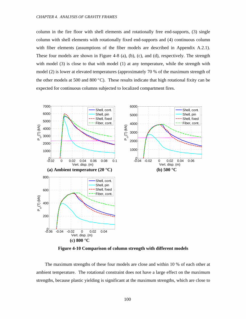
CHAPTER 4. ANALYSIS OF GRAVITY FRAMES
100
column in the fire floor with shell elements and rotationally free end-supports, (3) single
column with shell elements with rotationally fixed end-supports and (4) continuous column
with fiber elements (assumptions of the fiber models are described in Appendix A.2.1).
These four models are shown in Figure 4-8 (a), (b), (c), and (d), respectively. The strength
with model (3) is close to that with model (1) at any temperature, while the strength with
model (2) is lower at elevated temperatures (approximately 70 % of the maximum strength of
the other models at 500 and 800 °C). These results indicate that high rotational fixity can be
expected for continuous columns subjected to localized compartment fires.
-0.02 0 0.02 0.04 0.06 0.08 0.10
1000
2000
3000
4000
5000
6000
7000
Vert. disp. (m)
Pcr
(T) (
kN)
Shell, cont.Shell, pinShell, fixedFiber, cont.
-0.04 -0.02 0 0.02 0.04 0.060
1000
2000
3000
4000
5000
6000
Vert. disp. (m)
Pcr
(T) (
kN)
Shell, cont.Shell, pinShell, fixedFiber, cont.
(a) Ambient temperature (20 °C) (b) 500 °C
-0.06 -0.04 -0.02 0 0.02 0.040
200
400
600
800
Vert. disp. (m)
Pcr
(T) (
kN)
Shell, cont.Shell, pinShell, fixedFiber, cont.
(c) 800 °C Figure 4-10 Comparison of column strength with different models
The maximum strengths of these four models are close and within 10 % of each other at
ambient temperature. The rotational constraint does not have a large effect on the maximum
strengths, because plastic yielding is significant at the maximum strengths, which are close to

CHAPTER 4. ANALYSIS OF GRAVITY FRAMES
101
the perfectly plastic axial force ( 0yAF = 6120 kN, where A is the cross-sectional area and
0yF is the yield strength at ambient temperature). Post buckling strength, however,
significantly drops in model (3) compared with models (1) and (2). The remained rotational
stiffness at the end hinges helps the strength at this stage. The deformed shape of the column
at the post-buckling stage is shown in Figure 4-11.
The maximum strength with model (4), which cannot simulate local buckling, is slightly
higher than that with model (1); however the differences are limited (within 2 % at elevated
temperatures). Post buckling strength is higher with model (4) without local buckling.
Further comparison between shell and fiber models including flexural buckling about the
strong axis and lateral torsional buckling are shown in Appendix A.2.
Figure 4-11 Post buckling deformation of shell element model
4.2.3.3 Modeling of Constraint Springs
Realistic evaluation of the constraint spring properties in Figure 4-7(b) is a key for the
simulations using this subassembly. The spring represents the vertical stiffness and strength
of the floor framing of levels above the critical column. Since the springs at every floor
shown in Figure 4-7(a) are identical, the condensed spring stiffness and strength in Figure
4-7(b) is simply obtained by multiplying the spring properties for a single floor by the
number of the floors that are supported by the gravity column at the fire floor. The vertical

CHAPTER 4. ANALYSIS OF GRAVITY FRAMES
102
stiffness and strength of a single floor is evaluated using beam models shown in Figure 4-12.
As shown in the structural floor plan in Figure 4-1, four beams with three sections connect to
the interior gravity column: Beam a, b and c as shown in Table 4-1. Details of the
connections between the column and beams are shown in Figure 4-2. Since the span of
Beam a (W14×22) and b (W14×38) is identical (6.4 m) and the difference in sectional
properties is relatively small, the properties for the connection of Beam a are also used for
Beam b. Therefore, two analytical models for Beam a/b and c are created. As shown in
Figure 4-12, the model consists of three components: a steel composite beam, an inelastic
rotational spring for the shear tab bolted connection, and an elastic longitudinal constraint
spring by floor structure.
Figure 4-12 Analysis model of beams for vertical spring stiffness of floor structure
The steel beam is modeled with shell elements and inelastic longitudinal springs are used
to model the concrete slab. The effective width of the concrete slab is assumed equal to one-
quarter of the span length in accordance with AISC (1995). A bilinear stress-strain curve
with 0.1 % strain hardening is used for the steel. Concrete properties are adopted from
Eurocode 2 (EC2, 1993). No reinforcement and no tensile strength are assumed for the
concrete slab, which is common in US practice (although reinforcement may be placed near
columns depending on design). The strength of the steel deck is also ignored.
Inelastic rotational springs are located at the ends of the composite beam representing
the stiffness and strength of shear tab bolted connections. An experimental study for this

CHAPTER 4. ANALYSIS OF GRAVITY FRAMES
103
type of connection has been performed by Liu and Astaneh-Asl (2004). Their study focuses
on the rotational and shear behavior of the connection, including the composite effect of the
concrete slab and steel beam under cyclic seismic load. Although the loading in this study is
not cyclic, the results are still applicable to evaluate the vertical stiffness and strength of the
floor structure. According to the proposed modeling by Liu and Astaneh-Asl, the inelastic
rotational properties of shear-tab connections for Beams a/b and c (Figure 4-1 and Figure
4-2) are calculated and shown in Figure 4-13.
Figure 4-13 Rotational properties of shear-tab connections
A large difference in positive and negative moment capacities are observed due to the
different contribution of the concrete slab in each loading direction. The maximum positive
moment capacity is controlled by the bolted connection failure in tension (Point 1 in Figure
4-13), where the corresponding compression force couple is carried by the concrete slab.
Bolts located at lower part of the shear-tab connections fail under the maximum moment
capacity (Point 1), while bolts higher in the connection retain some strength provide
additional rotational capacity (Point 2-3). The maximum rotational deformation (Point 3) is
controlled by binding of the beam flange and column. The contribution of the concrete slab
is very limited and is ignored for the negative moment capacity (Point 4), which is obtained
from the maximum moment resistance provided by the bolt group.
The longitudinal constraint stiffness of each beam is calculated from the analysis model
of the floor structure shown in Figure 4-14(a). Here, the floor system is modeled with a
combination of axial struts, representing the steel beams, and shell finite elements,
representing the concrete slab. Both beam strut and slab finite element models are elastic and

CHAPTER 4. ANALYSIS OF GRAVITY FRAMES
104
the stiffness of the concrete, which work for tension as well as compression, is assumed to be
50 % of the initial stiffness for compression (8.0 GPa). A vertical displacement is imposed at
the location of the interior gravity column and it induces, through membrane action,
horizontal displacements at the far ends of the connecting beams. Shown in Figure 4-14(b) is
the vertical section of beam a on column line C indicated in Figure 4-14(a).
(a) Floor model
(b) X-X section
Figure 4-14 Analysis model of floor structure for in-plane stiffness calculation
The axial force of Beam a, ap , and corresponding horizontal displacements, aδ , at the
far ends of the beams are monitored, and the effective spring stiffness of the floor is obtained
by comparing aδ and aHp , which is the horizontal component of axial force of Beam a.

CHAPTER 4. ANALYSIS OF GRAVITY FRAMES
105
Shown in Figure 4-15 are the relationship between aδ and aHp for Beam a as well as those
for Beam b and c. The constraint stiffness of Beam c is relatively small compared to beam a
and b, because there is no continuous slab for Beam c. The lateral displacement and force
under an imposed vertical displacement of 0.4 m are marked with circles in the figure. As it
will be shown later (Figure 4-22), 0.4 m is almost the maximum vertical displacement studied
in this paper. The equivalent secant elastic stiffness of the longitudinal constraint spring of
the beams is defined and superimposed in the plot. The elastic stiffness is 125,000 kN/m for
Beam a and b, and is 54,000 kN/m for Beam c. This simulation is approximate, because
accurate calculation of this constraint stiffness is difficult and involves many issues such as
nonlinear behavior of the concrete slab, the stud connections between the steel beams and
concrete slab, the steel connections, and 3D effects from the stiffness of the vertical
components including the lateral resisting system.
0 0.005 0.01 0.015 0.020
500
1000
1500
2000
2500
Horiz. disp. (m)
Rea
ctio
n (k
N)
Bm a,b modelBm c modelBm a analysisBm b analysisBm c analysis
Figure 4-15 Longitudinal constraint stiffness of beams
The properties of the vertical spring of each floor structure shown in Figure 4-7(a) are
computed in the following steps: (1) the property of the longitudinal constraint springs at the
end of the connecting beams to the interior gravity column are prepared by computing a
model of the floor structure shown in Figure 4-14, (2) the vertical stiffness and strength of
each composite beam are calculated under imposed vertical displacement (Figure 4-12), (3)
the vertical spring for each floor is calculated by combining the contribution of each beam in
the floor, (4) longitudinal elongation of the column at fourth and higher floors is assumed as
negligible and the condensed vertical spring, shown in Figure 4-7(b), is obtained by simply
multiplying the spring property of each floor.

CHAPTER 4. ANALYSIS OF GRAVITY FRAMES
106
Shown in Figure 4-16 are the vertical spring properties of the floor structure and
contribution of Beam a, b and c, where the vertical stiffness and strength of Beam a is
practically identical to that of Beam b. The limit-state condition of the vertical resistance of
the floor diaphragm (Figure 4-12) is connection failure for all beams. The critical vertical
strengths are 37 kN for Beam a and b, and 100 kN for Beam c (indicated with circles in
Figure 4-16). At the limit-state, the resultant of the axial and shear forces reaches the
capacity of the connections, which are 393 kN (web plate bearing) for Beam a and b, and 955
kN (shear-tab plate bearing or bolt shear failure) for Beam c. The limit-state is simply
evaluated based on this resultant and is not coupled with rotational behavior. The initial
vertical stiffness of each floor structure is about 0.15 % of the longitudinal stiffness of the
gravity column per floor, 0E A L , where A is the cross-sectional area and L is the floor
height. This relatively low stiffness of the vertical spring with respect to the column supports
the condensation of the upper floor columns to the simplified model shown in Figure 4-7(b).
0 0.1 0.2 0.3 0.4 0.5 0.60
50
100
150
200
Δ (m)
P (k
N)
Beam a, bBeam cTotal
Figure 4-16 Vertical resistance of floor structure
4.2.4 Evaluation of Critical Temperatures
In this section, the vertical displacement under varied temperatures of the heated interior
gravity column shown in Figure 4-7(b) is numerically evaluated and the critical temperatures
are consequently obtained. The equilibrium equation of this system with respect to the
vertical displacement under a given temperature can be written as:

CHAPTER 4. ANALYSIS OF GRAVITY FRAMES
107
( ) ( , )s c gP P L dT T PαΔ + Δ + = (4.1)
,where sP is the force resisted by the inelastic vertical spring, cP is vertical load carrying
capacity of the column, and gP is gravity load composed of dead and live load. Therefore,
the left-hand-side of this equation is the resistance and the right-hand-side is the force. Δ is
the vertical displacement of the heated column (relative displacement of third floor level to
the second floor level). Δ is measured as positive in the downward direction. The origin is
the top of the column under dead and live load without thermal expansion. L is the length of
the heated column (4 m), α is the thermal expansion coefficient (1.4×10⁻⁵ m/°C), T is the
temperature, and dT is the increment of temperature (=T - 20 °C). sP is a function of the
vertical displacement, Δ , and the resistance curves as shown in Figure 4-16. cP is a function
of Δ , T , and the column behavior. The effect of thermal expansion is included in this
resistant capacity by adding L dTα to Δ . Relationships between cP and Δ for a given T
are shown in Figure 4-9. Because the thermal expansion effect is included in cP , the applied
force gP is a constant in this equation and calculated with mean dead and live loads (102.5 %
and 25 % of the design loads, respectively (Ellingwood, 1983).
Three conditions of the vertical constraint spring on column response are studied: (1)
without a constraint spring, (2) with an elastic constraint spring, and (3) with an inelastic
constraint spring. The stiffness of the elastic constraint spring is defined as the initial
stiffness of the inelastic spring. In the case of the study without the constraint spring, there is
no sP term in Eq. (4.1). Therefore, for this case, equilibrium combinations of temperature
and the vertical displacement are obtained from the intersections of the resistant curves, cP
with respect to Δ under given T and the axial load level gP shown in Figure 4-9. Similarly,
results for the case with elastic and inelastic springs are shown in Figure 4-17. Plotted on the
vertical axis of each figure is resistance of the system (the left-hand-side of Eq. (4.1)) at
ambient and elevated (100-800 °C) temperatures resulting from the constraint spring
properties, shown in Figure 4-16, and the column resistance. The response for the case with
an elastic spring is shown in Figure 4-17(a) and with an inelastic spring in Figure 4-17(b).
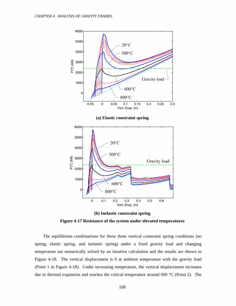
CHAPTER 4. ANALYSIS OF GRAVITY FRAMES
108
(a) Elastic constraint spring
(b) Inelastic constraint spring
Figure 4-17 Resistance of the system under elevated temperatures
The equilibrium combinations for these three vertical constraint spring conditions (no
spring, elastic spring, and inelastic spring) under a fixed gravity load and changing
temperature are numerically solved by an iterative calculation and the results are shown in
Figure 4-18. The vertical displacement is 0 at ambient temperature with the gravity load
(Point 1 in Figure 4-18). Under increasing temperature, the vertical displacement increases
due to thermal expansion and reaches the critical temperature around 600 °C (Point 2). The

CHAPTER 4. ANALYSIS OF GRAVITY FRAMES
109
critical temperatures for the study cases with and without the constraint springs are 598 °C
and 599 °C, respectively, and the constraint effect is very limited. The equilibrium points are
further obtained under decreasing temperature (Point 3); however, the structure will not
generally reach these points since the structure will become unstable at the peak points.
However, in the case with an elastic spring, the equilibrium temperature decreases from the
critical temperature at Point 2 and turns to increase again at around 500 °C. Eventually, it
increases to equilibrium at a temperature higher than the initial critical temperature. Under
simply increasing temperature, the displacement “snaps-though” from Point 2 to 4.
Assuming the constraint spring stays elastic and continues to pick up load, the equilibrium
temperature keeps increasing indefinitely. The gravity load is eventually all carried by the
elastic spring. At this stage, the building may not function due to the large vertical
displacement (about 0.2 m). However, the possibility of preventing the progressive collapse
of the building is an important benefit of this behavior.
Figure 4-18 Vertical displacement of the interior column under elevated temperatures
This snap-through type behavior is difficult to numerically evaluate. In this research, it
is possible by limiting degrees of freedom in structural systems (i.e., one degree of vertical
freedom for the interior gravity column). This approach is not generally scalable to more
complicated structural systems with more degrees of freedom. However, as the purpose of

CHAPTER 4. ANALYSIS OF GRAVITY FRAMES
110
this study is to examine the nature of gravity column behavior in frames, the simplified
approach provides a practical way to track the problem.
As is evident from Figure 4-18, the effect of the vertical inelastic constraint spring is not
significant for the critical temperature in the ten story case study building. In order to
examine further this issue, two other office buildings with different numbers of stories are
studied. The floor plan is identical to the benchmark design shown in Figure 4-1; and the
geometry of the fire compartment, fire scenario, beam sections, and location of heated
interior column are assumed to be the same. The numbers of stories of these buildings are 5
and 20. The fire floor is the second floor in both cases. The heated interior gravity column
sections at the fire floor are designed as W10×49 and W14×233 (Table 4-2) and factored load
ratios of these columns are 0.76 and 0.77 for 5- and 20-story buildings, respectively. The
corresponding factored load ratio in the original 10-story building design is 0.77. Thus this
ratio is comparable in all the three buildings. The critical temperatures crT with and without
consideration of constraint of springs are similarly simulated with analysis model shown in
Figure 4-7(b), and summarized in Table 4-3.
Table 4-2 Section sizes of columns in 5- and 20-story buildings (mm)
Number of story Section h wt fb ft
5 W10×49 253 8.6 254 14.2 20 W14×233 393 22.6 399 36.0
Table 4-3 Critical temperatures with different number of building stories
Number of story
Column section
Slenderness ratio
crT with constraint (°C)
crT without constraint (°C)
Difference (°C)
5 W10×49 61.4 594 600 -6 10 W14×90 42.3 598 599 -1 20 W14×233 38.8 620 612 +12
The spring enhances the critical temperature for the 5-story building by about 6 %, and it
deteriorates it by about 12 % for the 20-story building. The difference is not significant in
either case. This is because the vertical displacements at the limit-state are small
(longitudinal deformation of the column due to thermal expansion and material deterioration
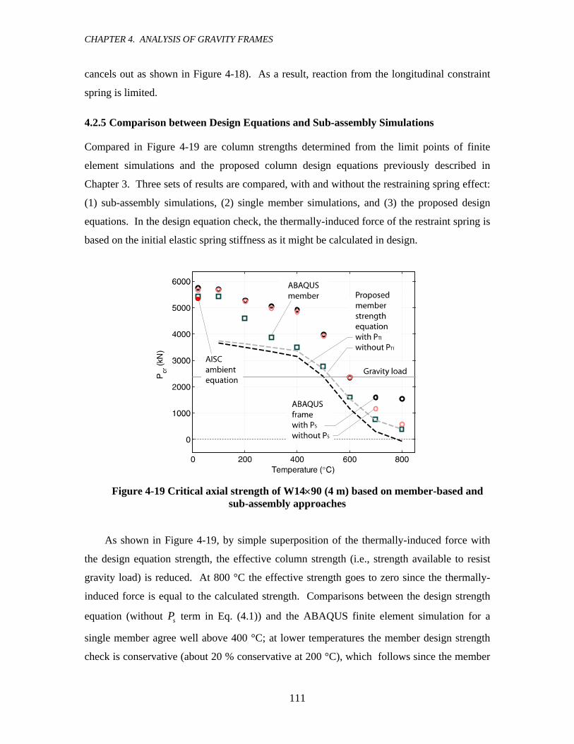
CHAPTER 4. ANALYSIS OF GRAVITY FRAMES
111
cancels out as shown in Figure 4-18). As a result, reaction from the longitudinal constraint
spring is limited.
4.2.5 Comparison between Design Equations and Sub-assembly Simulations
Compared in Figure 4-19 are column strengths determined from the limit points of finite
element simulations and the proposed column design equations previously described in
Chapter 3. Three sets of results are compared, with and without the restraining spring effect:
(1) sub-assembly simulations, (2) single member simulations, and (3) the proposed design
equations. In the design equation check, the thermally-induced force of the restraint spring is
based on the initial elastic spring stiffness as it might be calculated in design.
Figure 4-19 Critical axial strength of W14×90 (4 m) based on member-based and
sub-assembly approaches
As shown in Figure 4-19, by simple superposition of the thermally-induced force with
the design equation strength, the effective column strength (i.e., strength available to resist
gravity load) is reduced. At 800 °C the effective strength goes to zero since the thermally-
induced force is equal to the calculated strength. Comparisons between the design strength
equation (without sP term in Eq. (4.1)) and the ABAQUS finite element simulation for a
single member agree well above 400 °C; at lower temperatures the member design strength
check is conservative (about 20 % conservative at 200 °C), which follows since the member

CHAPTER 4. ANALYSIS OF GRAVITY FRAMES
112
design equation is specifically calibrated for elevated fire temperatures. Finally, comparing
the ABAQUS simulation results between the single member and the sub-assembly with and
without the restraining force ( sP ) yields the following observations: (1) the rotational
restraint provided by the columns above and below the heated floor have a significant
beneficial effect at temperatures above 200 °C (up to a 40 % increase at 400 °C), (2) the
restraining spring effect is negligible for temperatures below 700 °C, and (3) above 700 °C
the restraining spring helps to preserve the system capacity, provided that the restraining
elements have sufficient strength.
4.2.6 Improvement of Structural Robustness
It is observed from Figure 4-16 that resistance of the vertical constraint spring is controlled
by the capacity of the bolted shear-tab connections. This observation suggests that
strengthening of the connections may be an effective method for improving the collapse
resistance of the structural system. Two alternative design options for improved connection
details for Beam a and b are suggested in Figure 4-20. Option A entails increasing the
number of bolts in the connections, while Option B entails providing continuous
reinforcement in the concrete slab. The reinforcement is expected to contribute to supporting
axial tensile force at the connection. Although special design details may be needed to
ensure the connection between the steel beam and the added slab reinforcement, it is likely
that the shear studs provided for composite beam action will be strong enough so as not to be
critical to the failure mechanism.
(a) Option A
(5-7/8 in bolts are assumed.) (b) Option B
(8-#4 reinforcement bars are assumed.)
Figure 4-20 Options for strengthened connections

CHAPTER 4. ANALYSIS OF GRAVITY FRAMES
113
Assuming that the strength of the proposed connection options is adequate, then the
critical failure mechanism for Beam a and b is likely to be steel beam yielding (without
contribution of the introduced reinforcement for Option B). Note that other failure
mechanisms, such as yielding of the shear-tab or fracture, must be considered to assume that
beam yielding controls the critical strength. Accordingly, the connection strengthening could
increase the calculated maximum vertical resistance of the floor structure from 162 kN to 377
kN.
Figure 4-21 Total vertical load carrying capacity with strengthened connection for
Beam a and b
Figure 4-22 Vertical displacement of the buckled column with improved beam
connection

CHAPTER 4. ANALYSIS OF GRAVITY FRAMES
114
Shown in Figure 4-21 are the resistance of the system under elevated temperatures (100-
800 °C), assuming strengthened connections for Beam a and b (not for Beam c). The
equilibrium combination of the temperature and vertical displacement is shown in Figure
4-22. The snap-through behavior is observed at approximately 600 °C, after which the
equilibrium point is regained at around 0.5 m of the vertical displacement. At this point, the
vertical load of the column is completely taken by the vertical spring, thus providing an
alternative load carrying path. Although this study is limited to static analysis, it suggests
that strengthening of connections could provide a more robust structural system, thereby
preventing complete collapse of the system.
4.2.7 Conclusions
The fire resistance of a gravity column in a 10-story composite steel building with office
occupancy is evaluated under a given localized fire scenario. An interior W-shape column
frame is heated in the fire and buckling of the column is the critical collapse mechanism.
Evaluation is carried out using a sub-assembly including the interior column with finite shell
elements and an inelastic vertical spring, which is calibrated to represent the stiffness and
strength of the surrounding floor framing.
Conclusions through this limited case study using the interior sub-assembly analysis
model for this archetypical steel-framed building are summarized in the following points:
1. The rotational restraint provided by the columns above and below the heated floor has a
significant beneficial effect at elevated temperatures (up to a 40 % increase at 400 °C).
2. The additional axial compression induced by vertical restrain of the gravity framing to
thermal elongation does not significantly reduce the critical load of the column (i.e., it is
reasonable to neglect the possible negative effects of the vertical restraint).
3. The vertical strength and stiffness provided by typical gravity framing is not sufficient to
provide an alternative load path once the critical column temperature is reached.
4. Details are suggested for how the gravity framing connections could be made more
robust (stronger) to provide sufficient strength to provide an alternative load path after
column buckling. However, this alternative load path would not engage until large (e.g.,
0.5m) deformations occur.

CHAPTER 4. ANALYSIS OF GRAVITY FRAMES
115
4.3 EVALUATION OF BEAM SUB-ASSEMBLY
Takagi, J., Deierlein, G.G. “Behavior and Limit-state Assessment of Steel Composite Beams under Localized Compartment Fire” (in preparation).
4.3.1 Summary
The behavior and strength limit-state of composite steel beams in a steel-framed building are
analytically evaluated under a localized compartment fire, considering the effects of the
shear-tab type bolted connections and the interaction of the heated beam and the surrounding
floor framing. The finite element models of the composite beams are composed of various
elements including shell elements for the steel beam, longitudinal springs of the concrete
slab, inelastic springs of the bolted connections, and a longitudinal constraint spring for the
in-plane floor diaphragm stiffness. The properties of the bolted connections are carefully
evaluated through comparison with existing experimental data, because simulations indicate
that connections are subjected to thermally-induced force and bolt shear failure is the critical
failure mode under the fire. Alternative design details for the connections are suggested and
the suggested improvements are validated by simulations. It is shown that composite beams
with the improved connections can survive to more than 800 °C (at the lower flange) if large
mid-span sagging (more than 20 % of the beam span) is accepted in the effect of the fire.
4.3.2 Introduction
Beam failure including failure of bolted connections is one of the typical failure mechanisms
of steel buildings under fires. Many researchers have studied the behavior and the strength
limit-state of steel beams under fire conditions using both analytical and experimental
approaches (Liu and Davies, 2001; Allam et al., 2002; Wainman and Kirby, 1988). In order to
evaluate realistic behavior of composite beams in building structures, the interaction between
the steel beams and other structural components (e.g., steel-concrete composite effect and
longitudinal deformation constraint by floor framing) must be considered (Bailey et al.,
1996b, Sanad et al., 2000, Baily, 2005). Composite steel beams with concrete slabs are a
very popular structural system in steel buildings. In addition to enhancing the stiffness of the
beams, concrete slabs contribute by controlling the steel temperature and by enabling the
development of membrane action when slab reinforcement is present. Constraint of
longitudinal deformation by floor framing is also influential to beam behavior. If the
constraint is high, axial compressive force is induced in the beams, which can cause buckling
CHAPTER 4. ANALYSIS OF GRAVITY FRAMES
116
and connection failures. However, the high axial constraint can also enable the development
of catenary action, which can provide an alternate load path.
In this research, the behavior and limit-state of beams under a fire are evaluated
considering the interaction with surrounding structural components in a benchmark steel-
framed office building. Secondary floor beams are the primary focus along with behavior of
shear-tab type bolted connections. The effect of the concrete slab is considered by
introducing inelastic longitudinal springs and the steel beams are modeled with finite shell
elements. The material properties of steel and concrete at elevated temperatures are adopted
from Eurocode. It is found that failure of the bolted connection dominates the limit-state of
typical beam design. Alternative design options to improve the critical strength are proposed
and the performance is numerically verified.
4.3.3 Analysis Model
4.3.3.1 Modeling of System
Finite element models created for the composite beams are composed of various elements,
including shell elements for the steel beam, longitudinal springs for the concrete slab,
inelastic springs for the bolted connections, and a longitudinal constraint spring for the floor
framing (Figure 4-23). This study focuses on the secondary beam (Beam a in the floor
framing plan in Figure 4-1) and vertical deformation of the supporting beam (Beam c) is
assumed as negligible (vertical displacements at the ends are fixed). The property of the
longitudinal constraint spring is obtained through independent simulations using an elastic
floor framing structural model. The properties of the longitudinal spring of the bolted
connections are carefully evaluated through calibration with existing experimental data.
Modeling of each structural element for the composite beam will be discussed in following
sections.

CHAPTER 4. ANALYSIS OF GRAVITY FRAMES
117
Figure 4-23 System of finite element composite beam model in floor framing
4.3.3.2 Modeling of Steel Beam
Three dimensional finite shell element models are created for the steel beams by using
commercial finite element analysis software, ABAQUS (Hibbitt, Karlsson & Sorensen, 2002).
The model assumptions are similar to those used in 4.2.3.2 for the interior column study and
some additional assumptions particularly applied for the beam model are described in the
following points:
1. Residual stress is not considered.
2. The temperature distribution in the composite section is defined based on reported
experimental data (Wainman and Kirby, 1988) as shown in Figure 4-24. The temperature
of the lower flange and lower three-quarters of web is defined as LT . The temperature of
the upper one-quarter of web is 0.9 LT , while that of the upper flange and concrete slab is
0.8 LT and 0.4 LT , respectively. The imposed temperatures change during analyses in
proportion to this fixed distribution mode through the cross-section. The temperature
distribution along the member length is assumed to be uniform.
3. The coefficient of thermal expansion is independent of temperature and assumed as
1.4×10⁻⁵ m/°C for both steel and concrete.
4. Out-of-plane (web plane) displacement and rotation about the longitudinal axis are fixed
at the center of the upper flange along with the length. Vertical displacement is fixed at

CHAPTER 4. ANALYSIS OF GRAVITY FRAMES
118
the center of the upper flange at the ends, and longitudinal displacement at these points is
free.
(Temperature at bolted connections is assumed as 0.9 LT .)
Figure 4-24 Temperature distribution of composite section
4.3.3.3 Modeling of Concrete Slab
Inelastic longitudinal springs are placed above the steel beam at the center of the concrete
slab. The length of each spring is 0.2 m and the end displacement of each spring is linked to
the beam section with a kinematic linear constraint as shown in Figure 4-23. The average
thickness of the concrete slab is 112.5 mm and the effective width described in AISC (2005)
is used for the cross-sectional area to calculate the spring properties. The stress-strain curves
of concrete at the elevated temperatures are adopted from Eurocode 2 (1993) (Figure 4-25).
No tensile strength is considered in the slab assuming that no reinforcement is placed in the
concrete slab, following typical construction practice in the US.
The property of the longitudinal spring of the concrete slab above the bolted connection
(two springs at the ends) is different from that of the other springs along the beam length.
Evaluation of the effective concrete slab length at the ends is not straightforward; however, it
is not highly influential to overall beam behavior and strict evaluation is not needed. This is
because these springs are normally subjected to stretching deformation due to end rotation,
such that no force is induced in the springs. The effective length of these springs is assumed
as 1.6 m, which is one-quarter of the beam span and eight times longer than the length of the
other slab springs. An alternative design option with reinforcement in the concrete slab is
studied later and 1.6 m is chosen to represent the embedment length of reinforcement.

CHAPTER 4. ANALYSIS OF GRAVITY FRAMES
119
0 0.005 0.01 0.015 0.02 0.025 0.030
0.2
0.4
0.6
0.8
1
StrainS
tress
/ C
ompr
essi
ve s
treng
th 20°C100°C200°C300°C400°C500°C
Figure 4-25 Compressive stress-strain curve of concrete
4.3.3.4 Modeling of Bolted Connection
Figure 4-26 shows a conceptual relationship between the longitudinal displacement of a beam
and temperature. As temperature increases, the beam elongates. At this stage, the beam does
not significantly deform (sag) and is subjected to compressive axial force. Further increasing
temperature induces significant deterioration of steel strength and stiffness, which leads to
loss of flexural stiffness of beams. This induces large deformation and the beams may act
like cables to resist load through catenary action. The effectiveness of catenary action
depends on the boundary conditions (e.g., longitudinal support at beam ends and strength of
the connections). At this stage, the beams are subjected to tensile axial force and the
longitudinal displacement may change direction (i.e., The beams pull inward).
Figure 4-26 Gravity load supporting systems of beams at elevated temperatures

CHAPTER 4. ANALYSIS OF GRAVITY FRAMES
120
Figure 4-27 shows a detail of a typical shear-tab bolted connection used for the secondary
beam (Beam a) in the benchmark building design (Figure 4-1). This type of connection is
usually designed for the shear force associated with gravity dead and live load at ambient
temperature. Under elevated temperatures, however, this type connection can be critical to
beam failure when subjected to high compressive or tensile force as shown in Figure 4-26.
Figure 4-27 Detail of beam connection
The behavior and strength of high-strength bolted connections at elevated temperatures
have been evaluated by Yu (2006). Shown in Figure 4-29 are force-displacement
relationships of a single shear bolted connection with an ASTM A325 high strength bolt and
9.5 mm (3/8 inch) thick Grade 50 plates (Figure 4-28). The mechanical tests were carried out
under constant elevated temperatures up to 800 °C (with increments at every 100 °C).
Figure 4-28 Single shear bolt test by Yu (2006)

CHAPTER 4. ANALYSIS OF GRAVITY FRAMES
121
0 5 10 15 20 25 30 35 400
50
100
150
Displacement (mm)
Load
(kN
)
25°C100°C200°C300°C400°C500°C600°C700°C800°C
(a) Edge distance 1.0DB
0 5 10 15 20 25 30 35 400
50
100
150
200
Displacement (mm)
Load
(kN
)
25°C100°C200°C300°C400°C500°C600°C700°C800°C
(a) Edge distance 1.5 DB
Figure 4-29 Load-displacement relationships of single shear connections by Yu (2006)
The distance between the center of the bolts and the edge of the plates is 22.2 and 33.3
mm (Figure 4-28), which are equivalent to 1.0 and 1.5 times the bolt diameter BD . The
failure mechanisms in this test are bolt shear and plate bearing. A rapid drop in post-capping
strength is observed in the force-displacement relationships at relatively low temperatures,
while post capping strength remains relatively high with ductile deformation at higher
temperatures. Pre-loading initial displacements up to 6 mm are observed. The reason for the

CHAPTER 4. ANALYSIS OF GRAVITY FRAMES
122
initial displacements is mainly thermal expansion of the specimen, which were set in the
furnace at ambient temperature and loaded at the specified elevated temperatures.
Yu (2006) also investigated the shear strength of bolts at elevated temperatures. Doubly
sheared ASTM A325 and A490 high strength bolts were tested with thick plates such that
deformation of plate bearing is negligible. Figure 4-30 shows the shear strength of ASTM
A325 bolts (strength per single shear) superimposed with the maximum strength of single
shear connections obtained from Figure 4-29. The strength of the single shear connections
with 1.0 BD and 1.5 BD edge distance at ambient temperature are approximately 50 % and 80
% of the bolt shear strength, respectively. This is because plate bearing is the dominating
failure mode for the single shear connections. However, the difference decreases at elevated
temperatures and there is almost no difference more than 500 °C. This means that bolt shear
failure is more critical at elevated temperatures than plate bearing. This is consistent with the
observation in the experiments by Yu.
0 200 400 600 8000
50
100
150
200
250
Temperature (°C)
Max
. she
ar s
treng
th (k
N)
conn. 1.0Dconn. 1.5Dbolt
Figure 4-30 Maximum single shear strength of A325 bolts by Yu (2006)
Three ASTM A325N bolts with 22.2 mm (7/8 inch) diameter are used for the connection
as shown in Figure 4-27. The force-displacement relationship of the longitudinal springs of
the bolted connections in Figure 4-23 is assumed as bilinear with post capping softening
(Figure 4-31). One longitudinal spring is used in the analysis model (Figure 4-23) instead of
multiple springs for each bolt in order to simplify the model system and avoid difficulty in
analytical convergence dealing with the strength softening. Three components of beam
deformation can cause shear deformation of each bolt at the shear-tab connections: (1)
longitudinal deformation of the beam, (2) rotational deformation the connection, and (3)

CHAPTER 4. ANALYSIS OF GRAVITY FRAMES
123
vertical shear deformation. Displacement of each bolt is varied considering possible
rotational deformation at the connection, while longitudinal deformation of the beam induces
the same horizontal relative displacement to each bolt.
Figure 4-31 Force-displacement relationship model of bolted connection
Parameters to represent this force-displacement relationship include peak strength
( )BP T , displacement at the peak strength BpΔ , and displacement at vanishing strength BeΔ
(Figure 4-31). BpΔ and BeΔ are assumed as independent of temperature, while BP is a
function of temperature as shown in Eq. (4.2).
0( ) ( )B yB B B R BnP T K T N C Rζ= (4.2)
where ( )yBK T is the reduction ratio of the bolt strength at elevated temperatures, which is
adopted from ECCS (2001). The values of ( )yBK T are compared with the reduction factors
of steel by EC3 in Figure 4-32 and Table 4-4. Bζ is an adjustment factor to account for the
non-uniform distribution of bolt forces due to rotation. BN is the number of the bolts (three).
RC is a ratio between the mean bolt shear strength and 0BnR , which is the nominal single
shear strength of bolt, and is calculated to be 160 kN according to AISC (2005). The value of
RC is calibrated with experimental data by Yu (2006) and is defined as 1.5. The detail of the
calibration is described later in 5.2.4.

CHAPTER 4. ANALYSIS OF GRAVITY FRAMES
124
Figure 4-32 Reduction factor of bolt strength by ECCS
Table 4-4 Values of reduction factor of bolt strength
Temperature °C (°F) ( )yBK T ( )yK T ( )pK T ( )EK T
20 (68) 1.000 1.000 1.000 1.000
100 (212) 0.968 1.000 1.000 1.000
200 (392) 0.935 1.000 0.807 0.900
300 (572) 0.903 1.000 0.613 0.800
400 (752) 0.775 1.000 0.420 0.700
500 (932) 0.550 0.780 0.360 0.600
600 (1112) 0.220 0.470 0.180 0.310
700 (1292) 0.100 0.230 0.075 0.130
800 (1472) 0.067 0.110 0.050 0.090
900 (1652) 0.033 0.060 0.038 0.068
1000 (1832) 0 0.040 0.025 0.045
1100 (2012) 0 0.020 0.013 0.023
1200 (2192) 0 0 0 0
The rotational displacement at the connection varies under the flexural deformation of
the beam. This rotation makes it difficult to evaluate the properties of the single longitudinal
spring for the bolted connection. In order to simplify the evaluation, the rotational
displacement at the bolted connection is assumed to be a constant and 0.05 radian. This
rotational displacement is observed at the limit-states in the typical beam simulations. This
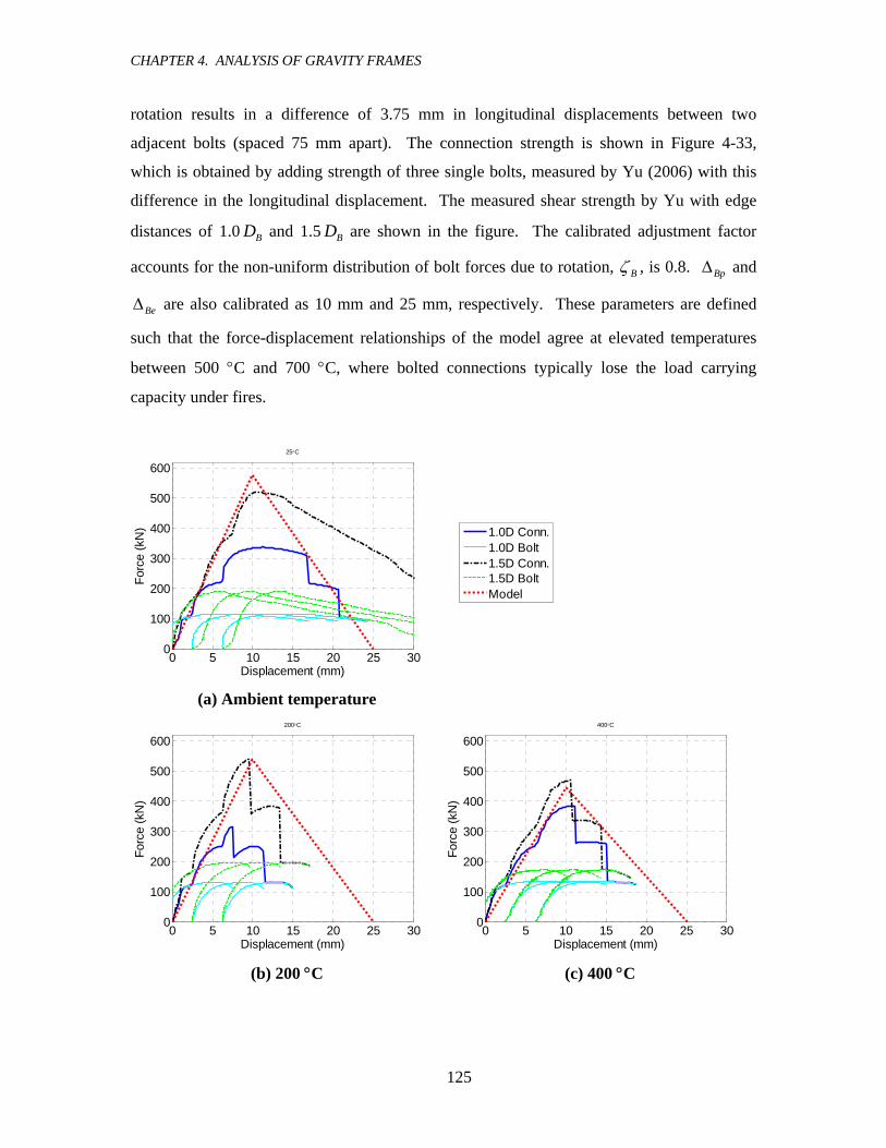
CHAPTER 4. ANALYSIS OF GRAVITY FRAMES
125
rotation results in a difference of 3.75 mm in longitudinal displacements between two
adjacent bolts (spaced 75 mm apart). The connection strength is shown in Figure 4-33,
which is obtained by adding strength of three single bolts, measured by Yu (2006) with this
difference in the longitudinal displacement. The measured shear strength by Yu with edge
distances of 1.0 BD and 1.5 BD are shown in the figure. The calibrated adjustment factor
accounts for the non-uniform distribution of bolt forces due to rotation, Bζ , is 0.8. BpΔ and
BeΔ are also calibrated as 10 mm and 25 mm, respectively. These parameters are defined
such that the force-displacement relationships of the model agree at elevated temperatures
between 500 °C and 700 °C, where bolted connections typically lose the load carrying
capacity under fires.
0 5 10 15 20 25 300
100
200
300
400
500
600
Displacement (mm)
Forc
e (k
N)
25°C
1.0D Conn.1.0D Bolt1.5D Conn.1.5D BoltModel
(a) Ambient temperature
0 5 10 15 20 25 300
100
200
300
400
500
600
Displacement (mm)
Forc
e (k
N)
200°C
0 5 10 15 20 25 300
100
200
300
400
500
600
Displacement (mm)
Forc
e (k
N)
400°C
(b) 200 °C (c) 400 °C

CHAPTER 4. ANALYSIS OF GRAVITY FRAMES
126
0 5 10 15 20 25 300
100
200
300
400
500
600
Displacement (mm)
Forc
e (k
N)
500°C
0 5 10 15 20 25 300
100
200
300
400
500
600
Displacement (mm)
Forc
e (k
N)
600°C
(d) 500 °C (e) 600 °C
0 5 10 15 20 25 300
100
200
300
400
500
600
Displacement (mm)
Forc
e (k
N)
700°C
0 5 10 15 20 25 300
100
200
300
400
500
600
Displacement (mm)
Forc
e (k
N)
800°C
(f) 700 °C (g) 800 °C
Figure 4-33 Comparison of force-displacement relationships of bolted connection between analysis model and test data by Yu (2006)
4.3.3.5 Modeling of Longitudinal Constraint by Floor Framing
Evaluation of the longitudinal constraint of steel beams in floor framings is difficult due to
the complex behavior of composite floor structures, such as inelastic response of the concrete
in the slab, stud connections between the concrete slab and steel beams, steel connections,
and three-dimensional (3D) interaction with vertical members. Also, the in-plain diaphragm
constraint stiffness depends on the location of the heated beams, geometry of the fire
compartment and fire scenarios. Consequently, the constraint stiffness is highly uncertain
and an approximate evaluation is performed in this section. Figure 4-34 shows an analysis
model of the floor structure composed of truss elements for the steel beams and shell
elements for the concrete slab. These elements are elastic and the elastic modulus of the shell

CHAPTER 4. ANALYSIS OF GRAVITY FRAMES
127
elements is set to 50 % of the initial compressive modulus of the concrete. Vertical load is
applied at the center of the heated secondary beams in the fire compartment and the
longitudinal constraint stiffness of the beams is calculated from the horizontal component of
tensile force of the beams ap (Figure 4-34(b)) and corresponding horizontal displacements
aδ . The calculated constraint stiffness of the four beams in the fire compartment is very
different for each beam. The average linear longitudinal constraint stiffness is approximately
1.0×10⁷ N/m. This is about 8 % of the elastic axial stiffness of a W14×22 beam with a length
of 6.4 m at ambient temperature. Although investigating the constraint stiffness in more
rigorous approaches is an interesting study subject, the approximated linear stiffness is used
in this research primarily focusing on understanding fundamental behavior of the composite
beams in frames under fire conditions. The sensitivity of this constraint stiffness to the
behavior of the composite beam will be investigated later.
Floor model
(b) Y-Y section
Figure 4-34 Analysis model for constraint stiffness

CHAPTER 4. ANALYSIS OF GRAVITY FRAMES
128
4.3.4 Evaluation of Behavior and Limit-state
4.3.4.1 Performance of Typical Design
Figure 4-35(a) shows relationships between lower flange temperature of the composite beam
and vertical displacement at the mid-span with and without consideration of longitudinal
constraint by the surrounding floor system. The critical temperatures are 634 °C and 660 °C
with and without the constraint, respectively. Loss of flexural stiffness due to steel yielding
is the failure mechanism of the beam without the constraint, while shear failure of the bolted
connection is critical for the beam with the constraint. The connection fails during beam
elongation (i.e., in the compression phase in Figure 4-26), after which the connection can no
longer supported the vertical shear force. The temperatures at the capping strength and
failure of the connection are marked in the Figure 4-35(a). Although the failure mechanisms
are different between these cases, the critical temperatures are about the same.
0 200 400 600 800-0.2
-0.15
-0.1
-0.05
0
Temperature (°C)
Mid
-spa
n di
spla
cem
ent.
(m)
With constraintWithout constraintCappingConn. failure
0 200 400 600 800-0.7
-0.6
-0.5
-0.4
-0.3
-0.2
-0.1
0
Temperature (°C)
Mid
-spa
n di
spla
cem
ent (
m)
With slabWithout slabCappingConn. failure
(a) Longitudinal constraint effect (b) Concrete slab effect
Figure 4-35 Mid-span displacement and modeling comparison
Another comparison is carried out investigating the effect of the concrete slab on the
behavior of the composite beam. Figure 4-35(b) shows mid-span displacement of the beams
at elevated temperatures with and without the longitudinal springs for the concrete floor slab.
It is observed that the mid-span displacement is smaller with the concrete slab but the critical
temperature is lower. This is because shear failure of the connection in the compression
phase (Figure 4-26) is critical for the beam with the concrete slab (longitudinal elongation
due to thermal expansion is larger with small sagging deformation with higher stiffness),

CHAPTER 4. ANALYSIS OF GRAVITY FRAMES
129
while connection failure in the tension phase is critical without the slab. Assessment of the
critical mechanism has a fair degree of uncertainty because of the underlying and uncertain
assumptions regarding the force-displacement relationship of the bolted connections and the
spring stiffness for the constraint of the floor structure. However, this study is useful for
analytically deriving possible failure mechanisms, which have not been fully examined in
past research, and the critical temperatures in typical composite beam design.
Analytical difficulties were found during these simulations due to the modeling of the
longitudinal springs of the bolted connections, which have bilinear force-displacement
relationships including post peak-strength softening (Figure 4-31). Analyses were often
aborted at the peak-strength and the post peak-strength behavior was not properly simulated.
In order to stabilize the simulation, an alternative analytical technique is introduced. As
shown in Figure 4-36, simulations were run with springs having perfect-plastic force-
displacement relationships instead of post peak-strength softening. Multiple perfect-plastic
models were prepared and run with different yielding strengths of the connection springs. A
post peak-strength equilibrium point was found in each simulation, and temperatures and
displacements at the equilibrium points were traced. Combinations of the temperatures and
displacements at the equilibrium points traced in this approach are not necessarily ordered by
simply increasing temperature, i.e., a critical temperature at connection failure can be lower
than that at the peak-strength as shown in Figure 4-35(b). This approach is computationally
intensive; however it provides the ability to simulate the post peak-strength behavior with
reasonable analytical stability under current modeling development. The simulations were
performed to investigate the behavior for research purposes; however, further modeling and
analytical development is desired for practical application.
Figure 4-36 Post peak-strength evaluation of bolted connection

CHAPTER 4. ANALYSIS OF GRAVITY FRAMES
130
4.3.4.2 Performance of Alternative Design
Longitudinal deformation of composite beam floor framing is constrained in most cases,
although the stiffness of the constraint varies. It is observed from Figure 4-35 that shear
failure of bolted connections is critical and improving the connections may be an effective
means to enhance the performance of composite beams against fires. Two alternative design
options for the connections are proposed: (1) using slotted bolt holes (Figure 4-37(a)) and (2)
placing continuous reinforcement in the concrete slab in addition to the slotted bolt holes
(Figure 4-37(a) and (b)).
As noted previously, critical failure mechanism for standard connection is shear failure
of bolted connection in the compression phase (Figure 4-35). The proposed design option (1)
is, therefore, to use slotted bolt holes, which allow beam elongation (Figure 4-37(a)). This
detail is designed such that the axial force is released at the bolted connections in the
compressive phase (Figure 4-26) but provides support in the tension phase. No horizontal
response is expected in the compressive phase and the size of the slot should be large enough
so as not to come into bearing under the maximum deformation. In the option (2),
reinforcement in the concrete slab increases the tension strength of the connections. The
temperature of the concrete slab is relatively low compared with the steel beam (Figure
4-24), such that the tension strength of the reinforcement remains high. This strength can
enhance the performance of the beam connections near the tension phase (Figure 4-26)
However, without combining with option (1), reinforcement alone would not improve the
critical temperature, because the failure mechanism remains shear failure of the connections.
2-#4 reinforcing bars are assumed.
(a) Slotted bolt hole (b) Continuous reinforcement
Figure 4-37 Proposed design options for bolted connections

CHAPTER 4. ANALYSIS OF GRAVITY FRAMES
131
Figure 4-38 compares analysis results of the typical composite beam and two proposed
alternative designs. Vertical displacement at mid-span and longitudinal relative displacement
at the spring of bolted connections (compression positive) are plotted in Figure 4-38(a) and
(b), respectively. The critical temperatures and failure mechanisms are summarized in Table
4-5. The critical temperature of the typical design is 634 °C with bolt shear failure due to
thermal elongation of the beam. The relative displacement of the bolted connection
significantly increases around 600 °C, once the relative displacement reaches the capping
point (0.01 m) (Figure 4-38(b)). Increasing the number of bolts at the connection would not
significantly improve the critical temperature, because thermal elongation of the beam
without insulation imposes shear forces on the bolts and leads to bolt failure. On the other
hand, slotted bolt holes (alternative design option (1)) prevent this bolt shear failure and
improve the critical temperature by 95 °C to 729 °C. Mid-span displacement increases
dramatically near the critical temperature, as flexural stiffness and strength of the beam is
lost. The maximum relative displacement of the bolted connection in this case is
approximately 0.03 m at 695 °C. The relative displacement decreases at the higher
temperature. The current analytical algorithm cannot further trace this behavior; however,
there may still be equilibrium points at higher temperatures under a fully developed tension
system (catenary system with large deformation).
0 200 400 600 800-0.5
-0.4
-0.3
-0.2
-0.1
0
Temperature (°C)
Mid
-spa
n di
spla
cem
ent (
m)
TypicalSlotted holeSlotted hole + rebarCappingConn. failure
0 200 400 600 8000
0.01
0.02
0.03
0.04
Temperature (°C)
Dis
plac
emen
t at c
onne
ctio
n (m
) TypicalSlotted holeSlotted hole + rebarCappingConn. failure
(a) Mid-span displacement (b) Longitudinal relative displacement at the connection
Figure 4-38 Performance of composite beams with alternative design options for the connections
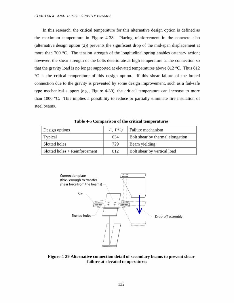
CHAPTER 4. ANALYSIS OF GRAVITY FRAMES
132
In this research, the critical temperature for this alternative design option is defined as
the maximum temperature in Figure 4-38. Placing reinforcement in the concrete slab
(alternative design option (2)) prevents the significant drop of the mid-span displacement at
more than 700 °C. The tension strength of the longitudinal spring enables catenary action;
however, the shear strength of the bolts deteriorate at high temperature at the connection so
that the gravity load is no longer supported at elevated temperatures above 812 °C. Thus 812
°C is the critical temperature of this design option. If this shear failure of the bolted
connection due to the gravity is prevented by some design improvement, such as a fail-safe
type mechanical support (e.g., Figure 4-39), the critical temperature can increase to more
than 1000 °C. This implies a possibility to reduce or partially eliminate fire insulation of
steel beams.
Table 4-5 Comparison of the critical temperatures
Design options crT (°C) Failure mechanism
Typical 634 Bolt shear by thermal elongation Slotted holes 729 Beam yielding Slotted holes + Reinforcement 812 Bolt shear by vertical load
Figure 4-39 Alternative connection detail of secondary beams to prevent shear
failure at elevated temperatures

CHAPTER 4. ANALYSIS OF GRAVITY FRAMES
133
4.3.4.3 Effect of Longitudinal Constraint
Stiffness of the longitudinal constraint of beams can significantly vary depending on multiple
factors including fire scenario, location of heated beam, and analysis modeling. The stiffness
is not precisely calculated in this research; rather the primary focus is on overall structural
fire simulations of beams in steel-framed buildings. Lacking accurate data to validate the
constraint spring stiffness, the influence of the spring stiffness on beam behavior is
investigated. Figure 4-40(a) compares mid-span displacements by changing the constraint
stiffness (denoted as sK ) from 107 N/m to 106 N/m and 108 N/m, in addition to no constraint.
The constraint stiffness of 107 N/m is approximately 8 % of the elastic axial stiffness of
W14×22 beam (without concrete slab) with 6.4 m at ambient temperature. Therefore, 106
N/m and 108 N/m are equivalent to 0.8 % and 80 % of the beam stiffness, respectively. The
behavior with the longitudinal constraint stiffness of 106 N/m is almost identical to that
without the constraint (Figure 4-40(a)) and the failure mechanism is beam yielding. Shear
failure of bolts due to thermal elongation of the beam is the failure mechanism for the beam
with the constraint stiffness of 107 N/m and 108 N/m. The critical temperatures for these
cases are 634 °C and 586 °C, respectively, which are lower than that with the constraint
stiffness of 106 N/m (622 °C). The critical temperature is decreased under high longitudinal
constraint with the failure mechanism of bolt shear in beam elongation. The critical
temperatures are summarized in Table 4-6.
0 200 400 600 800-0.2
-0.15
-0.1
-0.05
0
Temperature (°C)
Mid
-spa
n di
spla
cem
ent (
m)
w/o constraintKs = 106 N/mKs = 107 N/mKs = 108 N/mCappingConn. failure
0 200 400 600 800
-0.5
-0.4
-0.3
-0.2
-0.1
0
Temperature (°C)
Mid
-spa
n di
spla
cem
ent (
m)
w/o constraintKs = 106 N/mKs = 107 N/mKs = 108 N/mConn. failure
(a) Typical design (b) Slotted holes + reinforcement
Figure 4-40 Influence of the longitudinal constraint stiffness
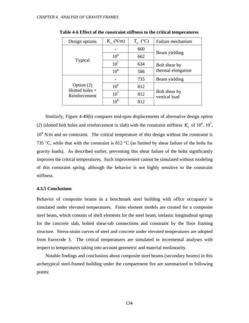
CHAPTER 4. ANALYSIS OF GRAVITY FRAMES
134
Table 4-6 Effect of the constraint stiffness to the critical temperatures
Design options sK (N/m) crT (°C) Failure mechanism
- 660 106 662
Beam yielding
107 634 Typical
108 586 Bolt shear by thermal elongation
- 735 Beam yielding 106 812 107 812
Option (2) Slotted holes + Reinforcement
108 812
Bolt shear by vertical load
Similarly, Figure 4-40(b) compares mid-span displacements of alternative design option
(2) (slotted bolt holes and reinforcement in slab) with the constraint stiffness sK of 106, 107,
108 N/m and no constraint. The critical temperature of this design without the constraint is
735 °C, while that with the constraint is 812 °C (as limited by shear failure of the bolts for
gravity loads). As described earlier, preventing this shear failure of the bolts significantly
improves the critical temperatures. Such improvement cannot be simulated without modeling
of this constraint spring, although the behavior is not highly sensitive to the constraint
stiffness.
4.3.5 Conclusions
Behavior of composite beams in a benchmark steel building with office occupancy is
simulated under elevated temperatures. Finite element models are created for a composite
steel beam, which consists of shell elements for the steel beam, inelastic longitudinal springs
for the concrete slab, bolted shear-tab connections and constraint by the floor framing
structure. Stress-strain curves of steel and concrete under elevated temperatures are adopted
from Eurocode 3. The critical temperatures are simulated in incremental analyses with
respect to temperatures taking into account geometric and material nonlinearity.
Notable findings and conclusions about composite steel beams (secondary beams) in this
archetypical steel-framed building under the compartment fire are summarized in following
points:

CHAPTER 4. ANALYSIS OF GRAVITY FRAMES
135
1. Failure of bolted shear-tab connections is critical. Alternative design options for the
connections are suggested using slotted bolt holes and installing continuous steel
reinforcement in the concrete slab. The improvement is analytically confirmed and the
critical temperatures can significantly increase from 634 °C to 812 °C at the lower flange
temperature. The failure mechanism changes from beam yielding to shear failure of the
bolts due to the gravity in this design improvement. Furthermore, preventing this bolt
failure against gravity can increase the critical temperature to more than 1000 °C. This
fact implies potential strength of composite steel beams in floor framings and possibilities
for new types of structural fire design.
2. The longitudinal constraint stiffness sK is approximately calculated using a relatively
simple elastic floor framing FEM model, which should pick up the most significant
aspects of the floor diaphragm behavior. The calculated lateral constraint stiffness is
about 8 % of the longitudinal stiffness of the steel beam (without composite effect). The
sensitivity of this constraint stiffness to the beam behavior is investigated for the typical
and improved alternative design with 0.1× sK and 10× sK . Overall, the behavior is not
very sensitive to the longitudinal stiffness; however, the critical temperature for the
alternative design is not improved without this constraint (i.e., crT = 735 °C without
constraint and 812 °C with constraint between 0.1× sK and 10× sK )
4.4 EVALUATION OF EXTERIOR COLUMN SUB-ASSEMBLY
4.4.1 Overview
The behavior and limit-states of the exterior column sub-assembly model are investigated in
this section. The model is composed of steel column and composite beam. The column is
modeled using shell finite elements, and the composite beam is modeled in the same way as
the beams in the beam study (Figure 4-23). The elevated temperatures of these members
vary depending on the assumed fire scenario, and structural simulation is carried out
incorporating the time-temperature relationships of the compartment fire based on Eurocode
1 (2002).
For the typical design, the critical failure mechanism during the fire is exterior column
buckling. Insulating the column changes the failure mechanism to a connection failure,
caused by large deformations and the associated tension forces in the beam. Alternative
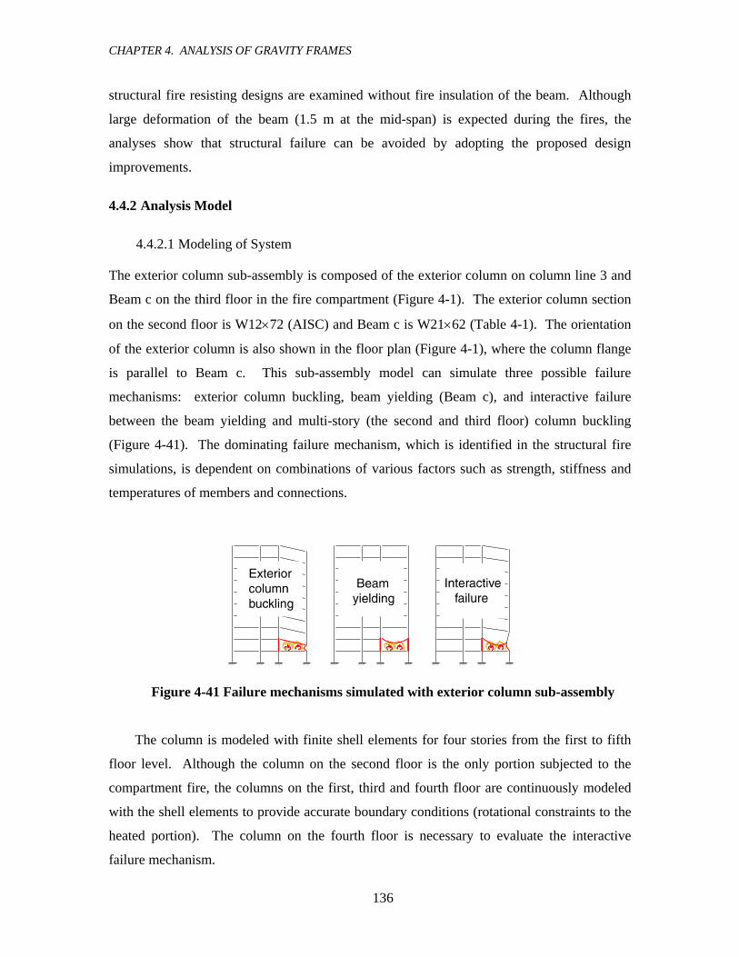
CHAPTER 4. ANALYSIS OF GRAVITY FRAMES
136
structural fire resisting designs are examined without fire insulation of the beam. Although
large deformation of the beam (1.5 m at the mid-span) is expected during the fires, the
analyses show that structural failure can be avoided by adopting the proposed design
improvements.
4.4.2 Analysis Model
4.4.2.1 Modeling of System
The exterior column sub-assembly is composed of the exterior column on column line 3 and
Beam c on the third floor in the fire compartment (Figure 4-1). The exterior column section
on the second floor is W12×72 (AISC) and Beam c is W21×62 (Table 4-1). The orientation
of the exterior column is also shown in the floor plan (Figure 4-1), where the column flange
is parallel to Beam c. This sub-assembly model can simulate three possible failure
mechanisms: exterior column buckling, beam yielding (Beam c), and interactive failure
between the beam yielding and multi-story (the second and third floor) column buckling
(Figure 4-41). The dominating failure mechanism, which is identified in the structural fire
simulations, is dependent on combinations of various factors such as strength, stiffness and
temperatures of members and connections.
Figure 4-41 Failure mechanisms simulated with exterior column sub-assembly
The column is modeled with finite shell elements for four stories from the first to fifth
floor level. Although the column on the second floor is the only portion subjected to the
compartment fire, the columns on the first, third and fourth floor are continuously modeled
with the shell elements to provide accurate boundary conditions (rotational constraints to the
heated portion). The column on the fourth floor is necessary to evaluate the interactive
failure mechanism.

CHAPTER 4. ANALYSIS OF GRAVITY FRAMES
137
Shown in Figure 4-42 is the finite shell element model of the exterior column sub-
assembly. The modeling of the steel column is essentially the same as that for the interior
column sub-assembly described in 4.2.3.2. The longitudinal constraint spring at the top of
the column is not included in this model, because it does not have a significant effect on the
critical strength, as found in simulations for the interior column sub-assembly. The modeling
of the steel beam and concrete slab is similar to that used for the simulations of the beam sub-
assembly, as described in 4.3.3.2 (also Appendix A.4.1). The modeling assumptions for the
concrete slab are discussed in 4.3.3.3 including the properties of concrete at elevated
temperature shown in Figure 4-25. The longitudinal constraint at the interior end of the
beams is assumed to be rigid. This is because the stiffness of the longitudinal constraint
developed in the beam is controlled by the exterior column, which is much more flexible than
the floor framing (e.g., the longitudinal constraint of the beam by the exterior column is
approximately 1.5×10⁶ N/m without strength deterioration of the column in the fire
compartment, while that by the floor framing calculated for the beam sub-assembly in
4.3.3.5. is on the order of 1.0×10⁷ N/m).
The constraint at the exterior end is based on only the bending stiffness of the exterior
column. As shown in Figure 4-43, the adjacent floor structure may significantly constrain the
lateral displacement at the exterior end through membrane action. However, in this case the
lateral stiffness would be coupled with the vertical displacement at the exterior column, and
including this effect is beyond the scope of the present analysis model.

CHAPTER 4. ANALYSIS OF GRAVITY FRAMES
138
Figure 4-42 System of exterior column sub-assembly model
Figure 4-43 Lateral constraint by floor slab with membrane action

CHAPTER 4. ANALYSIS OF GRAVITY FRAMES
139
To avoid the modeling complexity and uncertainty, the constraint membrane effect of
the floor structure is not considered in this exterior column sub-assembly model. This means
that interaction between frames in the east-west direction (e.g., column lines 3 and 4) is
neglected. If the fire compartment were larger (Figure 4-44(b)) and the frames on column
lines 1 to 6 behave similarly during the fire, neglecting the membrane effect is a more
convincing assumption. In this research, it is assumed that the membrane effect in the one-
bay fire is not significant and study on the effect is left for future work.
(a) One-bay compartment fire (b) Large compartment fire
Figure 4-44 Comparison of compartment fire for exterior column sub-assembly simulations
4.4.2.2 Modeling of Bolted Connection
In beam sub-assembly simulations, it is found that bolted connections are critical for beams
at elevated temperatures. Nonlinear longitudinal springs for the shear-tab bolted connections
are developed and validated using experimental data obtained by Yu (2006). A similar
approach is taken by introducing a longitudinal spring for the shear-tab bolted connections

CHAPTER 4. ANALYSIS OF GRAVITY FRAMES
140
between the exterior column and Beam c. Shown in Figure 4-45 is the detail of the shear-tab
connection. Five high-strength ASTM A325 bolts with 9.5 mm (3/8 inch) shear-tab plate are
used for the connection. As shown in the figure of the sub-assembly model (Figure 4-42), the
bolted connection is modeled as a combination of a slot and nonlinear spring. This
connection prevents longitudinal displacement of the beam and restraints the transverse
displacement. Therefore, shear failure of the connection due to the gravity load on the beam
is separately monitored from the longitudinal displacement and connection force.
Figure 4-45 Detail of exterior column connection
The properties of the nonlinear longitudinal spring are obtained in similar fashion to
those for the beam sub-assembly models. Due to analytical difficulty in including the peak-
strength softening, the bolted connection is modeled using a single longitudinal spring in the
simulations. Assuming bi-linear force-displacement relationships including post peak-
strength softening for the longitudinal spring (Figure 4-31), the temperature-dependent
relationships are calibrated with the experimental data obtained by Yu (2006) (single shear
connection test with 1.0 BD and 1.5 BD edge distance, where BD is the bolt diameter). The
rotational displacement at the connection, which leads to different displacements for each
bolt, makes it difficult to evaluate the properties of the single longitudinal spring for the
connection. For simplicity, a constant rotational displacement of 0.05 is assumed for the
evaluation of the spring property. The value of the constant rotational displacement is same
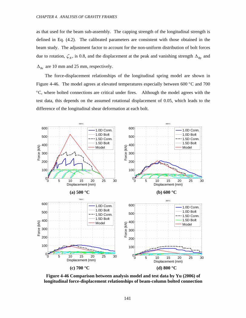
CHAPTER 4. ANALYSIS OF GRAVITY FRAMES
141
as that used for the beam sub-assembly. The capping strength of the longitudinal strength is
defined in Eq. (4.2). The calibrated parameters are consistent with those obtained in the
beam study. The adjustment factor to account for the non-uniform distribution of bolt forces
due to rotation, Bζ , is 0.8, and the displacement at the peak and vanishing strength BpΔ and
BeΔ are 10 mm and 25 mm, respectively.
The force-displacement relationships of the longitudinal spring model are shown in
Figure 4-46. The model agrees at elevated temperatures especially between 600 °C and 700
°C, where bolted connections are critical under fires. Although the model agrees with the
test data, this depends on the assumed rotational displacement of 0.05, which leads to the
difference of the longitudinal shear deformation at each bolt.
0 5 10 15 20 25 300
100
200
300
400
500
600
Displacement (mm)
Forc
e (k
N)
500°C
1.0D Conn.1.0D Bolt1.5D Conn.1.5D BoltModel
0 5 10 15 20 25 300
100
200
300
400
500
600
Displacement (mm)
Forc
e (k
N)
600°C
1.0D Conn.1.0D Bolt1.5D Conn.1.5D BoltModel
(a) 500 °C (b) 600 °C
0 5 10 15 20 25 300
100
200
300
400
500
600
Displacement (mm)
Forc
e (k
N)
700°C
1.0D Conn.1.0D Bolt1.5D Conn.1.5D BoltModel
0 5 10 15 20 25 300
100
200
300
400
500
600
Displacement (mm)
Forc
e (k
N)
800°C
1.0D Conn.1.0D Bolt1.5D Conn.1.5D BoltModel
(c) 700 °C (d) 800 °C
Figure 4-46 Comparison between analysis model and test data by Yu (2006) of longitudinal force-displacement relationships of beam-column bolted connection

CHAPTER 4. ANALYSIS OF GRAVITY FRAMES
142
4.4.3 Evaluation of Behavior and Limit-state
4.4.3.1 Basis of Simulations
Simulations of the exterior column sub-assembly are carried out in the time domain (i.e., time
is the primary parameter in simulations), while the simulations of the interior column and
beam sub-assemblies are performed in the temperature domain. The beam-column sub-
assembly response is described in terms of time since the beam and exterior column members
in this sub-assembly are subjected to different temperatures, depending on the type of
insulation and the gradient in the beam. Temperatures of the beam and exterior column are
obtained using the parametric fire (time-gas temperature) curve of Eurocode 1 (2002) and a
one-dimensional heat transfer analysis (by Buchanan 2002). The following input parameters
are assumed for the time-temperature curve: fuel load of 430 MJ/m2, fire compartment area
of 61 m2, total surface area of compartment equal to 235 m2, and opening factor of 0.05, and
a fire-fighting factor of 0.292. Where used, thermal insulation is assumed to be (or
equivalent to) 9.5 mm of gypsum wall board. Details of the parametric fire simulations and
numerical heat transfer approach are described in Appendix B.4.
Figure 4-47 Time-temperature relationships in a fire simulation
4.4.3.2 Simulation Results
Shown in Figure 4-48 are relationships between time, steel temperature, and displacements in
the sub-assembly simulation. The beam displacement is measured at mid-span (Figure
4-48(a)), and the horizontal column displacement is measured at the exterior column at the
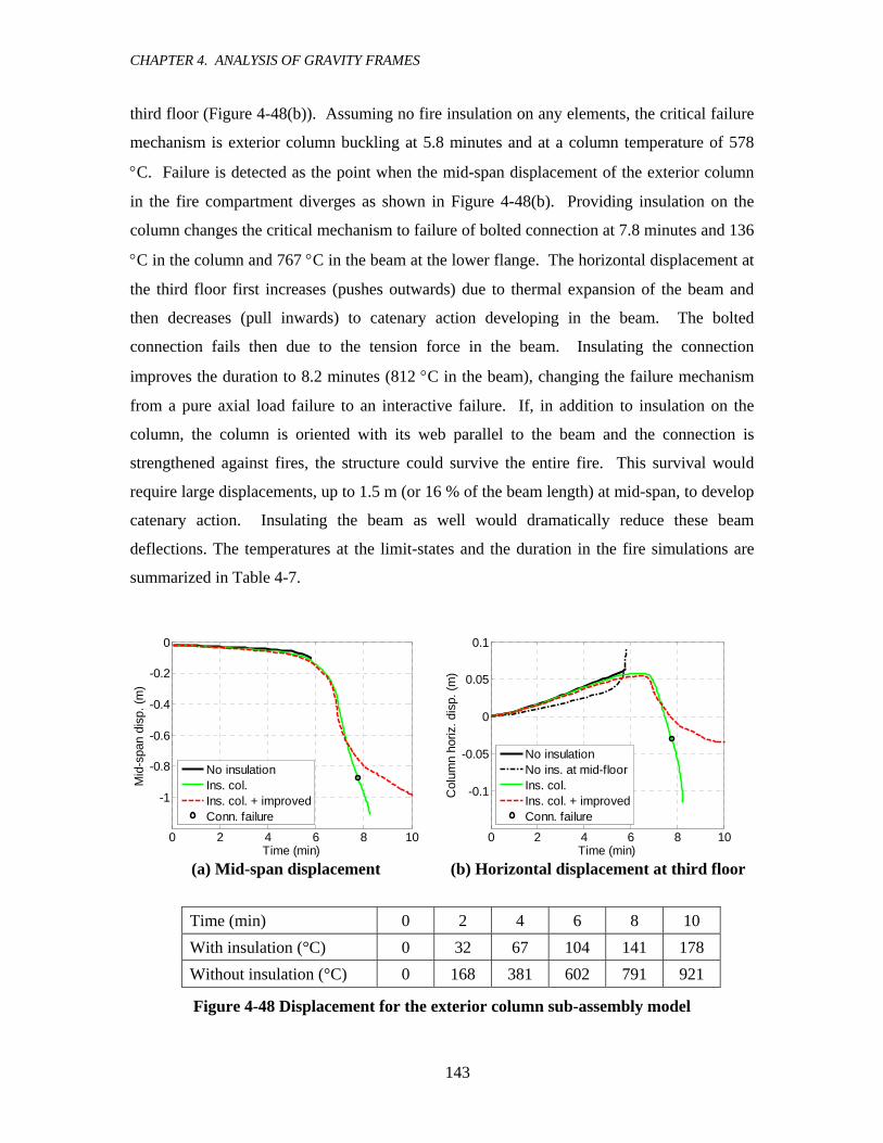
CHAPTER 4. ANALYSIS OF GRAVITY FRAMES
143
third floor (Figure 4-48(b)). Assuming no fire insulation on any elements, the critical failure
mechanism is exterior column buckling at 5.8 minutes and at a column temperature of 578
°C. Failure is detected as the point when the mid-span displacement of the exterior column
in the fire compartment diverges as shown in Figure 4-48(b). Providing insulation on the
column changes the critical mechanism to failure of bolted connection at 7.8 minutes and 136
°C in the column and 767 °C in the beam at the lower flange. The horizontal displacement at
the third floor first increases (pushes outwards) due to thermal expansion of the beam and
then decreases (pull inwards) to catenary action developing in the beam. The bolted
connection fails then due to the tension force in the beam. Insulating the connection
improves the duration to 8.2 minutes (812 °C in the beam), changing the failure mechanism
from a pure axial load failure to an interactive failure. If, in addition to insulation on the
column, the column is oriented with its web parallel to the beam and the connection is
strengthened against fires, the structure could survive the entire fire. This survival would
require large displacements, up to 1.5 m (or 16 % of the beam length) at mid-span, to develop
catenary action. Insulating the beam as well would dramatically reduce these beam
deflections. The temperatures at the limit-states and the duration in the fire simulations are
summarized in Table 4-7.
0 2 4 6 8 10
-1
-0.8
-0.6
-0.4
-0.2
0
Time (min)
Mid
-spa
n di
sp. (
m)
No insulationIns. col.Ins. col. + improvedConn. failure
0 2 4 6 8 10
-0.1
-0.05
0
0.05
0.1
Time (min)
Col
umn
horiz
. dis
p. (m
)
No insulationNo ins. at mid-floorIns. col.Ins. col. + improvedConn. failure
(a) Mid-span displacement (b) Horizontal displacement at third floor
Time (min) 0 2 4 6 8 10 With insulation (°C) 0 32 67 104 141 178 Without insulation (°C) 0 168 381 602 791 921
Figure 4-48 Displacement for the exterior column sub-assembly model
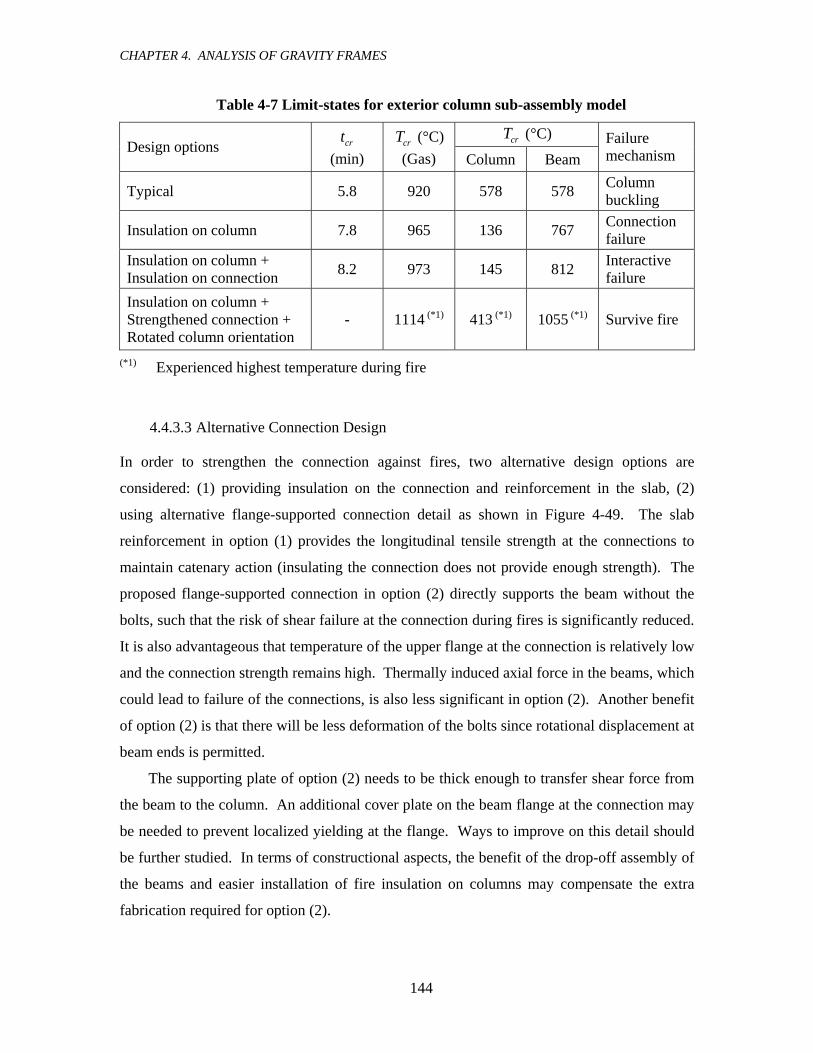
CHAPTER 4. ANALYSIS OF GRAVITY FRAMES
144
Table 4-7 Limit-states for exterior column sub-assembly model
crT (°C) Design options crt (min)
crT (°C) (Gas) Column Beam
Failure mechanism
Typical 5.8 920 578 578 Column buckling
Insulation on column 7.8 965 136 767 Connection failure
Insulation on column + Insulation on connection 8.2 973 145 812 Interactive
failure Insulation on column + Strengthened connection + Rotated column orientation
- 1114 (*1) 413 (*1) 1055 (*1) Survive fire
(*1) Experienced highest temperature during fire
4.4.3.3 Alternative Connection Design
In order to strengthen the connection against fires, two alternative design options are
considered: (1) providing insulation on the connection and reinforcement in the slab, (2)
using alternative flange-supported connection detail as shown in Figure 4-49. The slab
reinforcement in option (1) provides the longitudinal tensile strength at the connections to
maintain catenary action (insulating the connection does not provide enough strength). The
proposed flange-supported connection in option (2) directly supports the beam without the
bolts, such that the risk of shear failure at the connection during fires is significantly reduced.
It is also advantageous that temperature of the upper flange at the connection is relatively low
and the connection strength remains high. Thermally induced axial force in the beams, which
could lead to failure of the connections, is also less significant in option (2). Another benefit
of option (2) is that there will be less deformation of the bolts since rotational displacement at
beam ends is permitted.
The supporting plate of option (2) needs to be thick enough to transfer shear force from
the beam to the column. An additional cover plate on the beam flange at the connection may
be needed to prevent localized yielding at the flange. Ways to improve on this detail should
be further studied. In terms of constructional aspects, the benefit of the drop-off assembly of
the beams and easier installation of fire insulation on columns may compensate the extra
fabrication required for option (2).
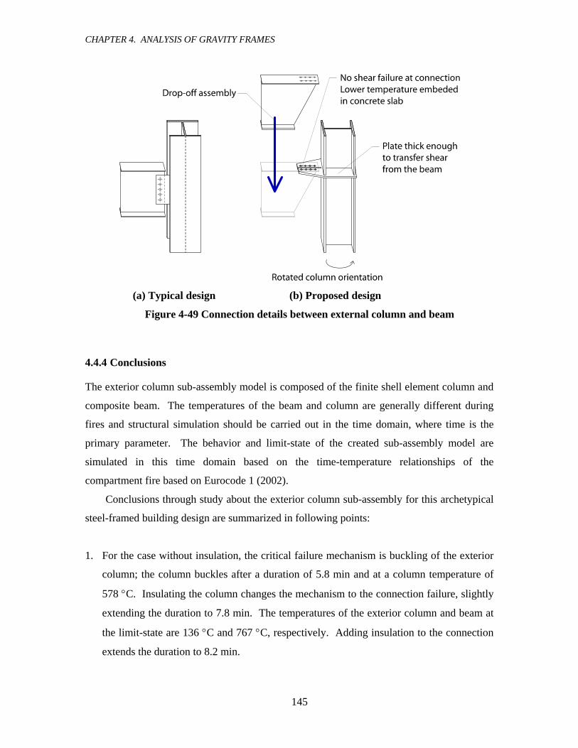
CHAPTER 4. ANALYSIS OF GRAVITY FRAMES
145
(a) Typical design (b) Proposed design
Figure 4-49 Connection details between external column and beam
4.4.4 Conclusions
The exterior column sub-assembly model is composed of the finite shell element column and
composite beam. The temperatures of the beam and column are generally different during
fires and structural simulation should be carried out in the time domain, where time is the
primary parameter. The behavior and limit-state of the created sub-assembly model are
simulated in this time domain based on the time-temperature relationships of the
compartment fire based on Eurocode 1 (2002).
Conclusions through study about the exterior column sub-assembly for this archetypical
steel-framed building design are summarized in following points:
1. For the case without insulation, the critical failure mechanism is buckling of the exterior
column; the column buckles after a duration of 5.8 min and at a column temperature of
578 °C. Insulating the column changes the mechanism to the connection failure, slightly
extending the duration to 7.8 min. The temperatures of the exterior column and beam at
the limit-state are 136 °C and 767 °C, respectively. Adding insulation to the connection
extends the duration to 8.2 min.

CHAPTER 4. ANALYSIS OF GRAVITY FRAMES
146
2. To fully survive the fire requires insulation on the exterior column, the connection, and
the beam. However, as an alternative to insulating the beam, other design options are
considered. The proposed design improvement includes rotating the column to provide
more longitudinal constraint to the beam and reinforcement in slab or alternative flange-
support connection detail as shown in Figure 4-49. Although large deformation of the
beam (1.5 m at the mid-span) is expected, the failure may be avoided without the fire
insulation on the beam by adopting the design improvement.
4.5 OVERALL LIMIT-STATE EVALUATION
Based on the limit-state analyses using the three sub-assembly models, the critical
mechanisms with different design conditions are summarized in Table 4-8. The critical time
is obtained from the time-temperature relationships of the steel members shown in Figure
4-47.
Table 4-8 Critical time, steel temperatures and failure mechanisms of sub-assemblies (time, min), [steel temperature, °C]
([Column temperature, Beam temperature] (°C) for exterior column sub-assembly)
Sub-assembly No insulation Insulation on columns (*1)
Insulation on columns (*1) +
Connection design (*2)
Interior column Column buckling (6.0), [599]
No failure (-), [-]
No failure (-), [-]
Exterior column and beam
Column buckling (5.8), [578, 578]
Connection failure (7.6), [136, 767]
Interactive failure (8.2), [145, 812]
Beam Connection failure (6.3), [634]
Connection failure (6.3), [634]
Connection failure (7.3), [729]
(*1) 9.5 mm gypsum board
(*2) Insulation on connections for the exterior column sub-assembly and slotted bolt holes for the beam sub-assembly
Without fire insulation, column buckling occurs early in the fire. For the interior
column, insulating the column avoids failure, whereas for the exterior assembly, insulating
the column (but not the beam or connection) only changes the critical mechanism to bolted
connection failure with a slightly longer endurance time (7.6 minutes versus 5.8 minutes).
Insulating the bolted connection allows slightly longer endurance (8.2 minutes versus 7.6
CHAPTER 4. ANALYSIS OF GRAVITY FRAMES
147
minutes) changing the failure mechanism from the connection failure to the interactive
failure. Insulating the beam (in addition to the column) avoids the failure of the exterior sub-
assembly. The sub-assembly failure may also be avoided without this fire insulation on the
beam by adopting design improvements, which are discussed in 4.4.3.3 (i.e., column rotation
and reinforcement in slab as shown in Figure 4-49). Regarding the beam sub-assembly,
insulating the connections does not prevent connection failure, if there is no insulation on
beams. This is because connection forces developed by resistance to thermal expansion of
the beams are often cause failure of the shear tab connections in compression. To prevent the
connection failure, alternative design options are discussed, such as using slotted bolt holes
and steel reinforcement in the concrete slab.
A key finding from this study is that there is some possibility of avoiding failure without
fire insulation on beams, while insulation on columns is essential. This finding is consistent
to the observations from the Cardington fire test (SCI, 2000; Kirby, 1997, 1998) and the
Broadgate Phase 8 fire (SCI, 1991) as described in Chapter 2. It is also found that failure of
the bolted connections is a critical failure mechanism, as well as the column buckling.
However, beam-drop failure due to the connection failure has not been reported in the past
fires and the Cardington fire test. In the Cardington fire test, shear failure of the bolts were
observed, but the beams did not fall, possibly due to the shear strength of the slabs.
Several possible reasons for the difference between this study and observations from
past fires are considered: (1) the uniform temperature of beams along the length assumed in
simulation may be a highly conservative assumption (non-uniform temperature distribution in
the beam length is expected in real fires and it would induce less significant longitudinal
deformation due to the thermal expansion), (2) bolted connections in the beams may have
lost the load transfer capacity in real fires; however, shear capacity of the concrete slab,
which is neglected in this study, may have been high enough to prevent the beam-drop, and
(3) the rotational deformation and longitudinal translation at the connections are not fully
coupled in the analyses and this may cause the difference between the simulation and reality.
4.6 CONCLUSIONS OF GRAVITY FRAME ANALYSIS
The sub-assembly simulations for a representative steel building support some of the
following observations and conclusions:

CHAPTER 4. ANALYSIS OF GRAVITY FRAMES
148
1. The restraint to vertical thermal column elongation provided by floors above the fire floor
does not significantly impact the strength limit state of the columns at the fire floor.
2. Column buckling is a critical mechanism and insulation on the columns is essential to
avoid collapse during building fires.
3. When the interior gravity column buckles during the fires, the surrounding structure of
the column is not strong enough to provide an alternative load-carrying path. However,
bracing the bolted connections between the column and connecting beams can provide an
alternative path and prevent the initiation of the global building collapse.
4. Failure of the bolted connections may occur due to thermal elongation of the beams.
Short of providing full beam insulation, beam failures can be controlled through
enhanced connection details that employ slotted bolt holes to permit the thermal
elongation and incorporate thermally protected reinforcement in the slab.
5. Protecting the connections with enhanced details and accepting large deformation
(sagging) during fires, the beams could survive more than 1000 °C by catenary action.
6. Insulating the exterior columns changes the failure mechanism from the single-story
buckling to the multi-story buckling associated with large deformation of the connecting
beam during the fires. Increasing the column stiffness for the frame by rotating the
column orientation (web is parallel to the frame) prevents this multi-story buckling and
the connection failure is then critical.
7. The connection between the exterior column and beam fails under tension force
associated with the catenary action. The slotted bolt holes, which are effective to prevent
the failure due to thermal elongation of the beam, are not helpful against this failure
mechanism. Therefore, other improved design options (e.g., reinforcement in the slab
and insulation on the connection) should be adopted for the connection.
These specific conclusions are based on a limited case study example and require
substantiation by further study. The proposed sub-assembly models are suggested as a means
to conduct such studies.

149
CHAPTER 5 PROBABILISTIC ASSESSMENT
5 PROBABILISTIC ASSESSMENT
5.1 OVERVIEW
In this chapter, probabilistic studies of steel structures under fires are performed for
individual members (columns) and the gravity frames of the benchmark building discussed in
Chapter 4. Statistical properties (mean and coefficient of variation) of characteristic
assessment parameters are defined based on previously published information and by
applying engineering judgment to estimate factors whose statistical information is unknown.
Sensitivity of the critical temperatures to these probabilistic parameters is evaluated for the
three sub-assembly structures introduced in Chapter 4. The uncertainty associated with fire
behavior is briefly addressed, but the primary focus of the assessment is on the structural
aspects. Probability of collapse of the sub-assemblies under given intensity (temperatures) is
assessed by the mean-value first-order second-moment (FOSM) method.
5.2 STRUCTURAL UNCERTAINTIES IN FIRE ENGINEERING
5.2.1 Summary of Statistical Data
Summarized in Table 5-1 is statistical information (mean and coefficient of variation, c.o.v.)
of input parameters used for structural simulations. This information will be used later in this
chapter for the probabilistic risk assessment. The parameters include the dead load, live load,
yield strength of steel at ambient and elevated temperatures ( 0yF and ( )yF T ), elastic
modulus of steel at ambient and elevated temperatures ( 0E and ( )E T ), strength (force-
displacement relationship) of the vertical constraint spring for the interior column ( sP ),
longitudinal constraint stiffness of the beams ( sK ), and the shear strength and deformation
capacity of the bolted connections ( BP and BΔ ).

CHAPTER 5. PROBABILISTIC ASSESSMENT
150
Table 5-1 Statistical data for uncertainties
μ (mean) δ (c.o.v) Type (*1) Reference
Dead load 4420 Pa (*2) 0.10 Normal Ellingwood, 1983
Live load 718 Pa (*2) 0.60 (*3) Gamma Ellingwood, 1983
0yF 1.05 ,y charF (*4) 0.10 Lognormal Ellingwood, 1983
( )yF T 0( )y yK T F 0.22 - Section 5.2.2
0E 200 GPa 0.06 Normal Ellingwood, 1983
( )E T 0( )EK T E 0.22 (*5) -
sP , vertical spring for the interior column
Figure 5-2 Figure 5-2 - Section 5.2.3
BP , strength of bolted connections
1.2 0( )yB B BnK T N R (*6) 0.29 - Section 5.2.4
BΔ , deformation capacity of bolted connections
Figure 5-5 0.25 - Section 5.2.6
sK , longitudinal constraint stiffness of the beams
1.0×10⁷ N/m (*7) Lognormal
(*1) Information about distribution types is reported for completeness but is not used in the probabilistic assessment by first-order second moment (FOSM) method.
(*2) Mean values of the dead and live loads are 102.5 % and 25 % of the unfactored design loads (4310 Pa (90 psf) for dead load and 2870 Pa (60 psf) for live load), respectively (Ellingwood, 1983).
(*3) c.o.v. of live load is defined as 0.40 to 0.80 (area-dependent) in Ellingwood (1983). The average value is taken.
(*4) ,y charF is the nominal specified value of the yield strength (345 MPa for Grade 50 steel).
(*5) Sufficient information has not been found. The c.o.v. was assumed to be the same as that for the yield strength, 0.22. This may be a conservative assumption considering that the yield strength and elastic modulus at ambient temperature have c.o.v.’s of 0.1 and 0.06, respectively.
(*6) BN is the number of bolts in a connection, and 0BnR the is nominal shear strength (bolt shear failure) of the bolts from AISC (2005). 0BnR is 160 kN for ASTM A325 bolts.
(*7) The mean stiffness is derived in Section 4.3.3.5. The 16 % and 84 % percentiles are assumed to be 400 % and 25 % of the median, respectively.
The statistical information about the loads (dead and live loads) and steel properties at
ambient temperature is obtained from Ellingwood (1983). The load properties under fire
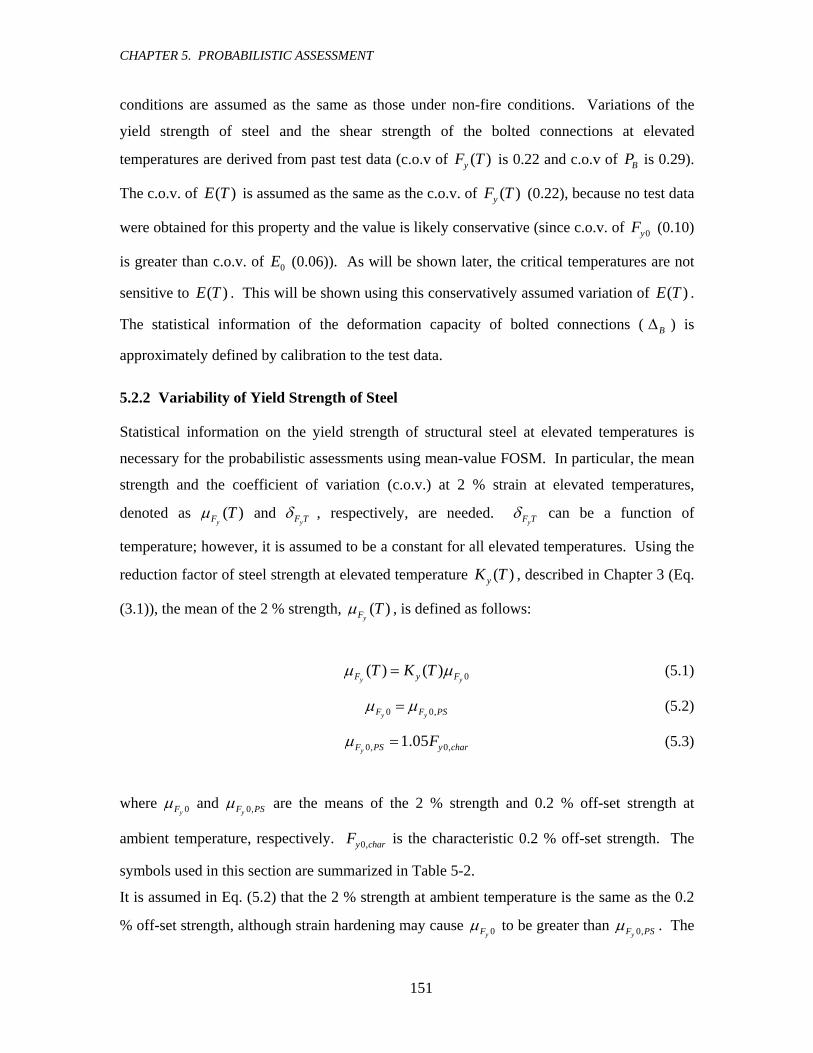
CHAPTER 5. PROBABILISTIC ASSESSMENT
151
conditions are assumed as the same as those under non-fire conditions. Variations of the
yield strength of steel and the shear strength of the bolted connections at elevated
temperatures are derived from past test data (c.o.v of ( )yF T is 0.22 and c.o.v of BP is 0.29).
The c.o.v. of ( )E T is assumed as the same as the c.o.v. of ( )yF T (0.22), because no test data
were obtained for this property and the value is likely conservative (since c.o.v. of 0yF (0.10)
is greater than c.o.v. of 0E (0.06)). As will be shown later, the critical temperatures are not
sensitive to ( )E T . This will be shown using this conservatively assumed variation of ( )E T .
The statistical information of the deformation capacity of bolted connections ( BΔ ) is
approximately defined by calibration to the test data.
5.2.2 Variability of Yield Strength of Steel
Statistical information on the yield strength of structural steel at elevated temperatures is
necessary for the probabilistic assessments using mean-value FOSM. In particular, the mean
strength and the coefficient of variation (c.o.v.) at 2 % strain at elevated temperatures,
denoted as ( )yF Tμ and
yF Tδ , respectively, are needed. yF Tδ can be a function of
temperature; however, it is assumed to be a constant for all elevated temperatures. Using the
reduction factor of steel strength at elevated temperature ( )yK T , described in Chapter 3 (Eq.
(3.1)), the mean of the 2 % strength, ( )yF Tμ , is defined as follows:
0( ) ( )y yF y FT K Tμ μ= (5.1)
0 0,y yF F PSμ μ= (5.2)
0, 0,1.05yF PS y charFμ = (5.3)
where 0yFμ and 0,yF PSμ are the means of the 2 % strength and 0.2 % off-set strength at
ambient temperature, respectively. 0,y charF is the characteristic 0.2 % off-set strength. The
symbols used in this section are summarized in Table 5-2.
It is assumed in Eq. (5.2) that the 2 % strength at ambient temperature is the same as the 0.2
% off-set strength, although strain hardening may cause 0yFμ to be greater than 0,yF PSμ . The
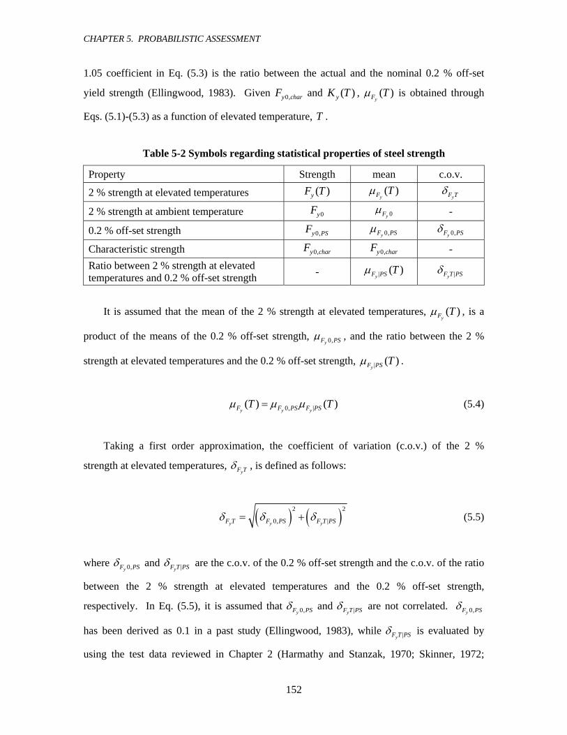
CHAPTER 5. PROBABILISTIC ASSESSMENT
152
1.05 coefficient in Eq. (5.3) is the ratio between the actual and the nominal 0.2 % off-set
yield strength (Ellingwood, 1983). Given 0,y charF and ( )yK T , ( )yF Tμ is obtained through
Eqs. (5.1)-(5.3) as a function of elevated temperature, T .
Table 5-2 Symbols regarding statistical properties of steel strength
Property Strength mean c.o.v.
2 % strength at elevated temperatures ( )yF T ( )yF Tμ
yF Tδ
2 % strength at ambient temperature 0yF 0yFμ -
0.2 % off-set strength 0,y PSF 0,yF PSμ 0,yF PSδ
Characteristic strength 0,y charF 0,y charF - Ratio between 2 % strength at elevated temperatures and 0.2 % off-set strength - | ( )
yF PS Tμ |yF T PSδ
It is assumed that the mean of the 2 % strength at elevated temperatures, ( )yF Tμ , is a
product of the means of the 0.2 % off-set strength, 0,yF PSμ , and the ratio between the 2 %
strength at elevated temperatures and the 0.2 % off-set strength, | ( )yF PS Tμ .
0, |( ) ( )y y yF F PS F PST Tμ μ μ= (5.4)
Taking a first order approximation, the coefficient of variation (c.o.v.) of the 2 %
strength at elevated temperatures, yF Tδ , is defined as follows:
( ) ( )2 2
0, |y y yF T F PS F T PSδ δ δ= + (5.5)
where 0,yF PSδ and |yF T PSδ are the c.o.v. of the 0.2 % off-set strength and the c.o.v. of the ratio
between the 2 % strength at elevated temperatures and the 0.2 % off-set strength,
respectively. In Eq. (5.5), it is assumed that 0,yF PSδ and |yF T PSδ are not correlated. 0,yF PSδ
has been derived as 0.1 in a past study (Ellingwood, 1983), while |yF T PSδ is evaluated by
using the test data reviewed in Chapter 2 (Harmathy and Stanzak, 1970; Skinner, 1972;

CHAPTER 5. PROBABILISTIC ASSESSMENT
153
DeFalco, 1974; Fujimoto et al.,1980, 1981; Kirby and Preston, 1988). Shown in Figure
5-1(a) is the measured strength at 1.5 % and 2.0 % strain at ambient and elevated
temperatures from 300 °C to 600 °C. The 1.5 % strength is investigated, because some of the
test data do not include strength at 2.0 % strain. The 1.5 and 2.0 % strengths are both
normalized with respect to the measured 0.2 % off-set yield strength in each test. Shown in
Figure 5-1(b) are the c.o.v.s of the 1.5 % and the 2.0 % strength. There are approximately 10
data points at each temperature. The effect of increasing temperature on the c.o.v. is
somewhat negligible until the temperature range between 500 °C and 600 °C, at which point
c.o.v. drastically increases.
0 100 200 300 400 500 6000
0.5
1
1.5
Temperature (°C)
Stre
ss /
Yie
ld s
tress
Mean at ε=1.5%Mean at ε=2.0%Data at ε=1.5%Data at ε=2.0%
0 100 200 300 400 500 6000
0.05
0.1
0.15
0.2
0.25
Temperature (°C)
c.o.
v
ε=1.5%ε=2.0%
(a) Mean (b) Coefficient of variation Figure 5-1 Variation of tested steel strength under elevated temperatures
Based on Figure 5-1(b), |yF T PSδ is assumed to be 0.2, which is close to the c.o.v. at 600
°C. This assumption is based on the fact that the critical temperatures of steel structures are
generally greater than 500 °C and, therefore, data at 600 °C are more important than data at
lower temperatures. |yF T PSδ is defined to be a constant value for elevated temperatures, since
this assumption greatly simplifies the probabilistic analyses given the limited data set.
Substituting 0.1 and 0.2 into 0,yF PSδ and |yF T PSδ in Eq. (5.5) yields 0.22 for yF Tδ .
5.2.3 Variability of Longitudinal Spring Stiffness for Interior Column
The properties of the vertical spring connected to the interior column in the benchmark
building were discussed in Section 4.2.3.3, and the relationship between the vertical

CHAPTER 5. PROBABILISTIC ASSESSMENT
154
displacement and reacting force of the spring was shown in Figure 4-16. The relationship
was evaluated approximately by introducing several assumptions and simplifications.
Therefore, precise statistical evaluation of this relationship is difficult. Possible variations of
this relationship are conservatively studied by considering the upper and lower bounds. In
Section 4.2.3.3, the vertical force-displacement relationship of the spring was calculated
using the analysis model shown in Figure 4-14. The model is composed of a composite
beam, bolted connection and the longitudinal constraint of the beam by the surrounding floor
structure. The variation of the properties of these components affects the calculated
properties of the vertical spring. Three factors of these components are considered to
influence the properties of the vertical spring: (1) the strength and (2) stiffness of the bolted
connection and (3) the stiffness of the longitudinal constraint spring for the beams. Possible
upper and lower bounds of these factors are discussed and the variation of the vertical spring
properties is evaluated.
The strength of the connections strongly influences the strength of the vertical spring,
because steel plate bearing (shear-tab or web plate) at the connections is the critical failure
mechanism of the vertical springs. Considering that the c.o.v. of the steel yield strength is
0.1 (Ellingwood, 1983) and the uncertainties introduced by other factors such as accuracy of
fabrication, influence from other failure mechanisms (e.g., bolt shear failure), and interactive
behavior with axial and rotational deformation, the c.o.v. of the connection strength is
assumed to be 0.2. Using this information, the upper and lower bounds of the connection
strength are assumed to be 120 % and 80 % of the typical (mean) strength.
The rotational spring stiffness of the bolted shear-tab connection strength influences the
stiffness of the vertical spring. Liu and Astaneh-Asl (2004) investigated the rotational
stiffness and strength of this type of connection, but they did not specifically address
statistical information about the rotational stiffness. They did, however, present data on key
rotational deformations and estimated their c.o.v. to be 0.2. Assuming this value is closely
related to the vertical spring stiffness and considering other uncertainties including
interaction with the axial force, the c.o.v. of the rotational stiffness of the connections is
assumed to be 0.3.
There is no significant statistical data available to characterize the uncertainty of the
horizontal elastic restraint stiffness that the floor structure provide to the beams. Past studies
have not focused on this property, which depends on many factors including building shape
and column location. Since generalizing statistical information is difficult, the upper and
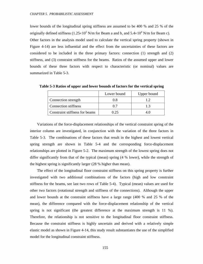
CHAPTER 5. PROBABILISTIC ASSESSMENT
155
lower bounds of the longitudinal spring stiffness are assumed to be 400 % and 25 % of the
originally defined stiffness (1.25×10⁵ N/m for Beam a and b, and 5.4×10⁴ N/m for Beam c).
Other factors in the analysis model used to calculate the vertical spring property (shown in
Figure 4-14) are less influential and the effect from the uncertainties of these factors are
considered to be included in the three primary factors: connection (1) strength and (2)
stiffness, and (3) constraint stiffness for the beams. Ratios of the assumed upper and lower
bounds of these three factors with respect to characteristic (or nominal) values are
summarized in Table 5-3.
Table 5-3 Ratios of upper and lower bounds of factors for the vertical spring
Lower bound Upper bound Connection strength 0.8 1.2 Connection stiffness 0.7 1.3 Constraint stiffness for beams 0.25 4.0
Variations of the force-displacement relationships of the vertical constraint spring of the
interior column are investigated, in conjunction with the variation of the three factors in
Table 5-3. The combinations of these factors that result in the highest and lowest vertical
spring strength are shown in Table 5-4 and the corresponding force-displacement
relationships are plotted in Figure 5-2. The maximum strength of the lowest spring does not
differ significantly from that of the typical (mean) spring (4 % lower), while the strength of
the highest spring is significantly larger (28 % higher than mean).
The effect of the longitudinal floor constraint stiffness on this spring property is further
investigated with two additional combinations of the factors (high and low constraint
stiffness for the beams, see last two rows of Table 5-4). Typical (mean) values are used for
other two factors (rotational strength and stiffness of the connections). Although the upper
and lower bounds at the constraint stiffness have a large range (400 % and 25 % of the
mean), the difference compared with the force-displacement relationship of the vertical
spring is not significant (the greatest difference at the maximum strength is 11 %).
Therefore, the relationship is not sensitive to the longitudinal floor constraint stiffness.
Because the constraint stiffness is highly uncertain and derived with a relatively simple
elastic model as shown in Figure 4-14, this study result substantiates the use of the simplified
model for the longitudinal constraint stiffness.

CHAPTER 5. PROBABILISTIC ASSESSMENT
156
Table 5-4 Combinations of factors for vertical spring of interior column
Connection strength
Connection stiffness
Constraint stiffness for beams
Typical Typ Typ Typ Highest UB LB LB Lowest LB UB UB
Higher beam constraint Typ Typ UB Lower beam constraint Typ Typ LB
(*) Typ: typical value (mean), UB: upper bound, and LB: lower bound
Figure 5-2 Variation of vertical spring properties
5.2.4 Variability of Shear Strength of Bolts
Yu (2006) experimentally investigated the performance of single shear bolted connections
with 22.2 mm (7/8 inch) diameter bolts (ASTM A325) and 9.5 mm (3/8 inch) thick Grade 50
plates. Plate bearing was observed as the failure mode at ambient temperature, while at
elevated temperatures the failure mode becomes shear failure of the bolts. This is due to the
more rapid strength deterioration of bolt capacity versus steel plate capacity (Figure 4-32 and
Table 4-4). Presuming that the bolt shear failure is the dominating failure mode for the
bolted shear-tab connections of the benchmark steel building, statistical properties of the bolt
shear strength at elevated temperatures are investigated in this section.
Yu (2006) also tested the shear strength of ASTM A325 and A490 bolts using thicker
steel plates so that bolt shear failure is the critical failure mode at all temperatures. Kirby

CHAPTER 5. PROBABILISTIC ASSESSMENT
157
(1995) tested the shear strength of British M20 Grade 8.8 high strength bolts in a similar way,
where two sets of tests (set A and C) were performed for different bolt steel compositions.
The shear strengths of the bolts from these tests (Yu 2006 and Kirby, 1995) are plotted in
Figure 5-3. Figure 5-3(a) shows the measured critical shear strength (double shear) of the
bolts at elevated temperatures up to 800 °C, and Figure 5-3(b) shows the strength normalized
with respect to the shear strength at ambient temperature and superimposed with the ECCS
(2001) reduction factor of bolt strength at elevated temperatures (the rule for the
normalization will be described later). Notice that the measured strengths around 300 °C are
slightly higher than that at ambient temperature, whereas the ECCS strength prediction
continuously decreases under elevated temperatures. Overall, the normalized test data agree
to ECCS within 20-30 % up to 700 °C.
0 200 400 600 8000
100
200
300
400
500
600
Temperature (°C)
She
ar s
treng
th (k
N)
Yu A490Yu A325Kirby AKirby B
0 200 400 600 8000
0.2
0.4
0.6
0.8
1
Temperature (°C)
Nor
mal
ized
she
ar s
treng
th
Yu A490Yu A325Kirby AKirby CECCS
(a) Measured shear strength (b) Normalized shear strength Figure 5-3 Shear strength of bolts at elevated temperatures
The nominal shear strength of high-strength bolted connections at ambient temperature
0BnR (bolt shear dominating strength) is defined in AISC (2005) as:
0Bn Bv BR F A= (5.6)
where BvF and BA are the ultimate shearing stress and the cross-sectional area of the
unthreaded part of the bolts, respectively. The British Grade 8.8 high strength bolts tested by
Kirby are equivalent to ASTM A325 and the nominal strength is evaluated in the same way

CHAPTER 5. PROBABILISTIC ASSESSMENT
158
for ASTM A325 based on AISC. The calculated BvF is 415 MPa (60 ksi) for both ASTM
A325 and British Grade 8.8, and 520 MPa (75 ksi) for ASTM A490. The tested bolts do not
include threads in the shear section, and BA is 388 mm2 (0.60 in2) for both ASTM A325 and
A490 with 9.5 mm (7/8 inch) diameter and 288 mm2 (0.45 in2) for British grade 8.8 M20
bolts. The 0BnR values based on Eq. (5.6) are 160 kN, 200 kN, and 120 kN for ASTM A325,
A490 22.2 mm diameter, and British grade 8.8 M20, respectively. The measured shear
strength of the bolts at ambient temperature is denoted as 0BtestR and the mean value is 0yBμ .
The ratio between 0yBμ and 0BnR is termed RC , as in the following equation.
0 0yB R BnC Rμ = (5.7)
where RC is found to be equal to 1.5 from the test data. The tested shear strength of bolts
shown in Figure 5-3(b) is normalized with respect to 0yBμ .
The statistical properties of the shear strength of bolted connections, which will be
needed later for the FOSM analysis, are the mean, yBμ , and c.o.v., yBδ . The mean at
ambient temperature 0yBμ is 0R BnC R , while c.o.v. at ambient temperature 0yBδ is obtained
from the test data by Yu (2006) and Kirby (1995) as 0.05. The mean at elevated
temperatures ( )yB Tμ is defined in the following equation using the reduction factor of bolted
connection strength ( )yBK T by ECCS (2001):
0( ) ( )yB yB yBT K Tμ μ= (5.8)
The values of ( )yBK T are shown in Figure 4-32 and Table 4-4 in Chapter 4. Under this
definition, ( )yB Tμ is not exactly equal to the mean of the normalized test data as shown in
Figure 5-3(b); however, it is close to the data and the formulated strength at elevated
temperatures consistent with ECCS prediction. Using ECCS is more advantageous than
using the test data for analytical manipulation.

CHAPTER 5. PROBABILISTIC ASSESSMENT
159
The c.o.v. of the shear strength of the bolts at elevated temperatures is assumed to be a
constant at any elevated temperature and denoted as yBTδ . The c.o.v. is defined in the
following equation as the variation of the tested bolt shear strength with respect to ( )yB Tμ at
temperatures between 400 °C and 700 °C.
{ }2
1( ) 1
1
n
Bi yB ii
yBT
R T
n
μδ =
−=
−
∑ for 400 °C ≤ iT ≤ 700 °C (5.9)
where BiR is the shear strength of i th test data point, iT is the temperature of the i th test
data point, and n is the number of tests performed at elevated temperatures between 400 °C
and 700 °C. The calculated value of yBTδ using Eq. (5.9) is 0.29. Shown in Figure 5-4 are
the test data of Figure 5-3, normalized by the mean strength defined in Eq. (5.8). The
assumed mean strength is lower than the measured mean strength at high temperature. This
is clearly observed at temperatures greater than 600 °C, although by this point the mean value
is only about 10 % to 15 % of the ambient strength values. The strength of the assumed
mean plus and minus the derived standard deviation is superimposed in the figure. The
assumed variation seems reasonable with the test data at elevated temperatures between 400
°C and 700 °C. The mean and c.o.v. of the bolt strength in this section are summarized in
Table 5-5.
0 200 400 600 800
0.6
0.8
1
1.2
1.4
1.6
1.8
2
2.2
Temperature (°C)
Nor
mal
ized
she
ar s
treng
th /
EC
CS Yu A490
Yu A325Kirby AKirby CECCSμ ± σ
Figure 5-4 Shear strength of bolts normalized with ECCS strength

CHAPTER 5. PROBABILISTIC ASSESSMENT
160
Table 5-5 Mean and c.o.v. of shear strength of bolts
yBμ (mean) yBδ (c.o.v.)
Ambient temperature 0R BnC R 0.05
Elevated temperatures 0( )yB yBK T μ 0.29
5.2.5 Variability of Longitudinal Strength of Springs for Bolted Connections
Bolted beam connections are modeled as inelastic longitudinal (axial) springs (see Figure 4-
23). As shown previously in Figure 4-31, the force-displacement relationships of the springs
are modeled using a bi-linear curve with a post peak-strength softening branch. The peak-
strength, ( )BP T , is defined by the following equation:
0( ) ( )B yB B B yBP T K T Nζ μ= (5.10)
where Bζ is an adjustment factor to account for the non-uniform distribution of bolt forces
due to rotation. BN is the number of the bolts. Assuming 0.05 for the rotational
displacement of the connection at the limit-state, the calibrated value of Bζ is 0.8, as
described in 4.3.3.4 and 4.4.2.2. Substituting Eq. (5.7) ( RC = 1.5) leads to the following
relationship between the mean strength of the longitudinal (axial) spring strength for the
connection at elevated temperatures and nominal shear strength of bolts at ambient
temperature:
0( ) 1.2 ( )B yB B BnP T K T N R= (5.11)
The c.o.v. of the peak strength of the connections is assumed to be the same as the c.o.v.
of the shear strength of bolts (0.29).
5.2.6 Variability of Deformation Capacity of Bolted Connections
While bolt shear failure is the critical mechanism for shear-tab connections, data from bolts
alone is not sufficient to evaluate the deformation characteristics of the connections, since the
beam web or bracket deformation is not negligible. Yu (2006) investigated force-

CHAPTER 5. PROBABILISTIC ASSESSMENT
161
displacement relationships of single shear bolted connections at elevated temperatures. The
tests provide useful information for the evaluation of the actual behavior of shear-tab
connections. As Yu’s tests were the only data available in this study, the variation of the
deformation capacity of the bolted connections is based on Yu’s study.
The force-displacement relationships of the longitudinal (axial) spring for the bolted
connections in the beam sub-assembly are obtained in Section 4.3.3.4. (Figure 4-33)
Although this model reasonably agrees with the test data, a range of variation is observed in
Figure 5-5, where the test data shown in the figure is identical to those in Figure 4-33. The
upper and lower bounds of the possible variation of the deformation capacity are assumed to
be 125 % and 75 % of the original. These upper and lower bound models are superimposed
on the data in Figure 5-5, assuming that the peak strength and proportion of BpΔ and BeΔ are
maintained. These upper and lower bounds compare well with the test data by Yu (2006)
(the bolt edge distance of 1.0 BD and 1.5 BD , where BD is bolt diameter), especially at 600
°C and 700 °C. Due to insufficient statistical data, the c.o.v. of the deformation capacity of
the longitudinal spring of the connection is not obtained in a formal manner. Rather, the
c.o.v. is assumed as equal to 0.25.

CHAPTER 5. PROBABILISTIC ASSESSMENT
162
0 5 10 15 20 25 30 350
50
100
150
200
250
300
350
Displacement (mm)
Forc
e (k
N)
500°C
1.0D Conn.1.5D Conn.Model μModel μ ± δ
0 5 10 15 20 25 30 350
50
100
150
200
250
300
350
Displacement (mm)
Forc
e (k
N)
600°C
1.0D Conn.1.5D Conn.Model μModel μ ± δ
(a) 500 °C (b) 600 °C
0 5 10 15 20 25 30 350
50
100
150
200
250
300
350
Displacement (mm)
Forc
e (k
N)
700°C
1.0D Conn.1.5D Conn.Model μModel μ ± δ
0 5 10 15 20 25 30 350
50
100
150
200
250
300
350
Displacement (mm)
Forc
e (k
N)
800°C
1.0D Conn.1.5D Conn.Model μModel μ ± δ
(c) 700 °C (d) 800 °C
Figure 5-5 Uncertainty of deformation capacity of bolted connection
5.2.7 Variability of Time-temperature Relationships in Compartment Fire
The behavior in buildings under fires is highly uncertain. The uncertainty is due to various
factors such as the geometry of buildings and fire compartments, the fire location, fuel load,
the materials in the fire compartments, and the firefighting activities. Assessing such
uncertain behavior is not a primary goal of this research. Nevertheless, to provide a more
complete perspective on the probabilistic issues, the variability of the time-temperature
relationships (gas and resulting steel temperatures) in the compartment fire is briefly
discussed in this section. In Section 4.4.3.1 (Figure 4-47), the compartment fire behavior of
the benchmark building was deterministically simulated and discussed using the parametric
fire curve obtained following Eurocode 1 (2002) with the following input parameters: fuel
load, 430 MJ/m2; fire compartment area, 61 m2; compartment total surface area, 235 m2;

CHAPTER 5. PROBABILISTIC ASSESSMENT
163
opening factor, 0.05; and fire fighting factor, 0.282. The thermal heat transfer follows an
approach described by Buchanan (2002), assuming 9.5 mm gypsum board for the insulated
members. Details of this parametric fire simulation and the time-step heat transfer approach
are described in Appendix B.4.1.
The fuel load, firefighting factor, and opening factor are influential factors for this fire
simulation. Consequently, they are they are the variables used to investigate the variation in
the fire simulation. Values of these factors are parametrically varied between the upper and
lower bounds as shown in Table 5-6. The resulting variations to the time versus temperature
curves are shown in Figure 5-6. The lower and upper bounds for the fuel load are defined as
mean plus and minus one standard deviation (the c.o.v. is 0.3 by EC1, 2002). Those for the
firefighting factor are the minimum and maximum value in EC1; and those for the opening
factors are calculated from possible window sizes for the office-type benchmark building.
Two cases are studied with different values for the upper bound of firefighting factor: 0.360
for poor conditions and 1.215 for extremely poor conditions (no safe access routes, no fire
fighting devices, and no smoke exhaust systems in staircases, as described in EC1).
Table 5-6 Band of influential factors for fire simulation
Typical Lower bound Upper bound Fuel load (MJ/m2) 420 301 559
Firefighting factor 0.282 0.149 0.360 (Poor condition) 1.215 (Extremely poor condition)
Opening factor 0.05 0.03 0.07

CHAPTER 5. PROBABILISTIC ASSESSMENT
164
(a) Normal firefighting condition
(b) Poor firefighting condition (different time scale from (a))
Figure 5-6 Variations of time-temperature relationships
The extremely poor firefighting condition delays the time to achieve the peak gas
temperature to more than 100 min and the total fire duration is more than 180 min. This long
fire duration increases the maximum steel temperature, especially for the insulated members.
The maximum temperatures of gas and steel are investigated under the three firefighting
conditions (good, poor, and extremely poor) with varied fuel load and opening factor. The

CHAPTER 5. PROBABILISTIC ASSESSMENT
165
results are summarized in Table 5-7. Large variation of the maximum temperatures is clearly
seen in this table, especially for insulated steel, where the lowest maximum temperature is
344 °C, while the highest is 1009 °C.
Table 5-7 Maximum temperatures in variation of fire simulation (°C)
Fire fighting condition Gas Steel with insulation
Steel without insulation
Good 913 344 777 Poor 1255 557 1244
Extremely poor 1311 1009 1307
Although the opening factor may be more certain once the building is designed, a wide
range between the upper and lower bounds is considered to account for variations of different
building designs. There are many other factors that influence fire simulations such as the
material of the fire compartment boundary and the extent of fire insulation, which greatly
affects steel temperatures. However, these factors are treated deterministically in this
introductory simulation. Full consideration of these probabilistic factors will provide even
greater variations; however simulating the variation is not a goal of this research. Rather the
probabilistic assessment in this study focuses on structural aspects (e.g., the probability of
structural failure under given temperatures).
5.3 PROBABILISTIC STUDIES
5.3.1 Sensitivity of Critical Temperatures to Uncertainties
Structural stability of the benchmark steel building under the localized compartment fire was
deterministically evaluated in Chapter 4. Three types of sub-assembly analysis models
(interior column, beam, and exterior column beam sub-assemblies) were introduced in order
to precisely simulate possible failure mechanisms. Using the statistical information about
structural parameters obtained in the previous section, sensitivities of the critical
temperatures for the three sub-assemblies to the uncertain parameters are evaluated in this
section.
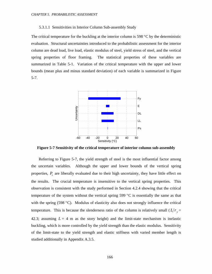
CHAPTER 5. PROBABILISTIC ASSESSMENT
166
5.3.1.1 Sensitivities in Interior Column Sub-assembly Study
The critical temperature for the buckling at the interior column is 598 °C by the deterministic
evaluation. Structural uncertainties introduced to the probabilistic assessment for the interior
column are dead load, live load, elastic modulus of steel, yield stress of steel, and the vertical
spring properties of floor framing. The statistical properties of these variables are
summarized in Table 5-1. Variation of the critical temperature with the upper and lower
bounds (mean plus and minus standard deviation) of each variable is summarized in Figure
5-7.
-60 -40 -20 0 20 40 60
Ps
LL
DL
E
Fy
Sensitivity (°C)
Unc
erta
inty
Figure 5-7 Sensitivity of the critical temperature of interior column sub-assembly
Referring to Figure 5-7, the yield strength of steel is the most influential factor among
the uncertain variables. Although the upper and lower bounds of the vertical spring
properties, sP are liberally evaluated due to their high uncertainty, they have little effect on
the results. The crucial temperature is insensitive to the vertical spring properties. This
observation is consistent with the study performed in Section 4.2.4 showing that the critical
temperature of the system without the vertical spring 599 °C is essentially the same as that
with the spring (598 °C). Modulus of elasticity also does not strongly influence the critical
temperature. This is because the slenderness ratio of the column is relatively small ( yL r =
42.3; assuming L = 4 m as the story height) and the limit-state mechanism is inelastic
buckling, which is more controlled by the yield strength than the elastic modulus. Sensitivity
of the limit-state to the yield strength and elastic stiffness with varied member length is
studied additionally in Appendix A.3.5.

CHAPTER 5. PROBABILISTIC ASSESSMENT
167
5.3.1.2 Sensitivities in Beam Sub-assembly Study
The critical mechanism of the beam sub-assembly at elevated temperatures is failure of the
bolted connections due to thermal expansion of the beam. Uncertain variables for this system
are the dead load (DL), live load (LL), deformation capacity ( BΔ ) and strength ( BP ) of bolted
connections, yield strength of steel ( yF ), and longitudinal constraint stiffness by the
surrounding floor framing ( sK ). Sensitivity of the critical temperature (634 °C) to these
variables is shown in Figure 5-8. The most influential factor is the deformation capacity of
the bolted connections ( BΔ ), which has about four times the influence of the connection
strength ( BP ). This implies that the axial force induced by the thermal expansion
overwhelms the strength of the bolted connections. As such, strengthening the connection is
a less effective method of preventing the connection failure than is providing greater
deformation capacity. Whereas the yield strength of steel at elevated temperatures is the
most influential factor for the interior column study, this is not the case for beams due to their
different failure mechanism. The elastic modulus of steel is not included in Figure 5-8;
however, it has been confirmed that the influence is limited.
-60 -40 -20 0 20 40 60
Sensitivity (°C)
Unc
erta
inty
Fy
ΔB
PB
DL
LL
Ks
Figure 5-8 Sensitivity of the critical temperature of beam sub-assembly
The sensitivity of the longitudinal spring stiffness from the floor framing, sK , is
relatively large (the second largest next to the deformation capacity of the bolted
connections). This result makes sense, because the longitudinal spring stiffness influences
the induced force at the connections and the critical mechanism is connection failure due to

CHAPTER 5. PROBABILISTIC ASSESSMENT
168
the thermal expansion of the beam. However, it should be noted that the upper and lower
bounds (mean plus and minus one standard deviation) of the spring stiffness were assumed to
be 400 % and 25 % of the standard (mean) stiffness Ksμ (=107 N/m). The higher spring
stiffness (4.0 Ksμ ) induces greater axial force at the connections and consequently decreases
the critical temperature. The lower spring stiffness increases the critical temperature and, in
fact, changes the failure mechanism from connection failure to beam yielding. Section
4.3.4.3. in Chapter 4 describes details of the behavior and variation of the critical
temperatures with different longitudinal spring stiffness (10 Ksμ and 0.1 Ksμ ). Combining the
results of this section and Section 4.3.4.3., the critical temperature, crT , is compared with sK
in Table 5-8. This table shows that crT does not change in proportion to sK . Considering
the uncertainty of sK and the wide range of the variation, crT is not strongly sensitive to sK .
Table 5-8 Critical temperature with various constraint stiffness
sK / Ksμ 0.1 0.25 1.0 4 10
crT (°C) 662 (+28) 642 (+8) 634 (±0) 605 (-29) 586 (-48)
5.3.1.3 Sensitivities in Exterior Column Sub-assembly Study
Behavior of the exterior column sub-assembly at elevated temperatures is deterministically
evaluated in Section 4.4.3. The critical mechanism is exterior column buckling, but
insulating the column changes the mechanism to connection failure. Temperatures of the
exterior column and the connecting beam (Beam c) are different and the limit-state is
evaluated in the time domain as shown in Chapter 4. Although sensitivity of the limit-state to
uncertain variables can also be evaluated in the time domain, the temperature domain is used
in this section in order to make the evaluation less dependent on the fire simulation and more
convenient to compare with other studies for the interior column and beam sub-assemblies.
The temperature of the exterior column and beam in the fire compartment at the limit-
state is defined as the critical temperature. The sensitivity of the critical temperature for the
buckling of exterior column (without fire insulation on the column) to the uncertain variables
is similar to that studied for the interior column sub-assembly. The sensitivity of the critical
temperature of the beam with fire insulation on the column is investigated in this section to

CHAPTER 5. PROBABILISTIC ASSESSMENT
169
determine the failure mechanism for the exterior column sub-assembly. The column
insulation prevents column buckling and the connection failure occurs at 5.8 min during the
particular compartment fire studied in Section 4.4.3.1. The critical temperatures at the limit-
state of the exterior column and beam are 136 °C and 767 °C, respectively. The uncertain
variables in this study are yield strength of steel ( yF ), deformation capacity ( BΔ ) and
strength ( BP ) of the bolted connection, dead load (DL), live load (LL). The sensitivity of the
critical temperature of the beam to these variables is shown in Figure 5-9. The most
influential variable is the yield strength of steel, yF . The strength of the bolted connection,
BP , is not as influential, although the connection failure is critical. This is because the
flexural stiffness loss of the beam changes the vertical load carrying mechanism from
bending to tension with catenary action (Figure 4-26), and the axial force overcomes the
connection strength.
Deformation capacity of the bolted connection does not influence the critical
temperature, which is in contrast to its significant effect for the beam sub-assembly. This
contrast is determined from the connection failure in different phases: the connection in the
beam sub-assembly fails in the compression phase (Figure 4-26), while that in the exterior
column sub-assembly fails in the tension phase. Connection failure in the compression phase
is deformation controlled because of thermal expansion, while that in the tension phase is
strength controlled because of the catenary action.
-60 -40 -20 0 20 40 60
Sensitivity (°C)
Unc
erta
inty
Fy
ΔB
PB
DL
LL
Figure 5-9 Sensitivity of the critical beam temperature of exterior column sub-
assembly

CHAPTER 5. PROBABILISTIC ASSESSMENT
170
5.3.2 Collapse Probabilities of Sub-assemblies given Temperatures
Using the statistical information shown in Table 5-1, the probability of failure is calculated
for the three sub-assemblies: interior column, beam, and exterior column. Deterministic
relationships between the gas and steel temperatures in the fire compartment are linearly
scaled for the temperature and the probability of failure under given elevated gas
temperatures is assessed. The deterministic temperature-time relationships are shown in
Figure 5-10, which is previously shown as Figure 4-47 based on the fire simulation
conditions described in 4.4.3.1. The mean-value first-order second-moment method (FOSM,
equations are shown in Appendix B.4) is used for the assessment, and all random variables
are assumed to be uncorrelated. A calculated cumulative distribution function (CDF) for
failure with respect to the gas temperature is shown in Figure 5-11. The CDFs are evaluated
for the three sub-assemblies (interior column sub-assembly with and without fire insulation,
beam sub-assembly without insulation, and exterior column sub-assembly with insulation on
the column and without insulation on the beam).
Of the three sub-assemblies, the critical collapse mechanism is buckling of the un-
insulated interior column, assuming that the exterior column is insulated. Figure 5-11 shows
that the failure of the beam sub-assembly (connection failure) can be critical (probability of
interior column buckling at 620 °C is about 50 %, while that of the connection failure at 620
°C is about 25 %). At 620 °C, the probability for the failure of the exterior column sub-
assembly is very low.
The maximum gas temperature in the fire simulation shown in Figure 5-10 is 1114 °C.
Therefore, the sub-assemblies would fail in most cases except the interior column sub-
assembly with fire insulation. Once performance of the proposed connection details is
precisely examined, additional study on the probability of failure for the improved beam and
exterior column sub-assembly design would provide interesting information.
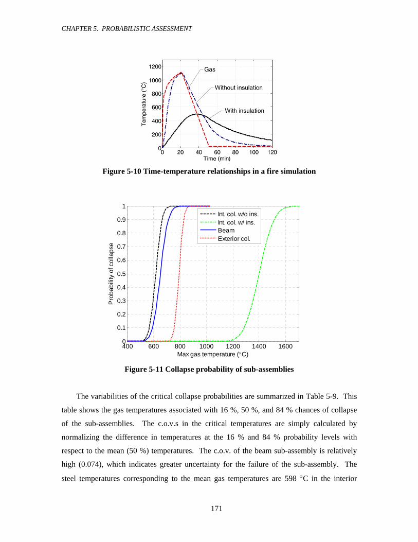
CHAPTER 5. PROBABILISTIC ASSESSMENT
171
Figure 5-10 Time-temperature relationships in a fire simulation
400 600 800 1000 1200 1400 16000
0.1
0.2
0.3
0.4
0.5
0.6
0.7
0.8
0.9
1
Max gas temperature (°C)
Pro
babi
lity
of c
olla
pse
Int. col. w/o ins.Int. col. w/ ins.BeamExterior col.
Figure 5-11 Collapse probability of sub-assemblies
The variabilities of the critical collapse probabilities are summarized in Table 5-9. This
table shows the gas temperatures associated with 16 %, 50 %, and 84 % chances of collapse
of the sub-assemblies. The c.o.v.s in the critical temperatures are simply calculated by
normalizing the difference in temperatures at the 16 % and 84 % probability levels with
respect to the mean (50 %) temperatures. The c.o.v. of the beam sub-assembly is relatively
high (0.074), which indicates greater uncertainty for the failure of the sub-assembly. The
steel temperatures corresponding to the mean gas temperatures are 598 °C in the interior

CHAPTER 5. PROBABILISTIC ASSESSMENT
172
column, 634 °C in the beam, 136 °C in the exterior column, and 767 °C in the beam in the
exterior column sub-assembly.
Table 5-9 Variability of the collapse probability with respect to gas temperature
Sub-assembly 16 percentile (°C)
mean (°C)
84 percentile (°C) c.o.v.
Interior column without insulation
577 (-39)
616 (±0)
655 (+39) 0.064
Interior column with insulation
1310 (-89)
1399 (±0)
1488 (+89) 0.064
Beam without insulation 604 (-48)
652 (±0)
700 (+48) 0.074
Exterior column with insulation on column and
without on beam
763 (-28)
792 (±0)
820 (+28) 0.036
5.3.3 Reliability of AISC-LRFD Fire Equation
The rationale of the simple design method in the AISC (2005) specification was discussed
and some alternative member-based design equations are proposed in Chapter 3. The AISC
method and proposed design equations are further evaluated in this section by introducing
probabilistic assessment concept.
Shown in Figure 5-12 is the fundamental concept of load and resistance in the load and
resistance factor design (LRFD) in AISC. The load and resistance are functions of random
variables and the expected load and resistance are their means. Nominal load and resistance
are separately and deterministically defined by the expected (mean) values for design.
Multiplying nominal values by factors gives the factored load and resistance, which are used
for the AISC strength evaluation according to the following equation:
n uR Qφ ≥ (5.12)
where, φ , nR , and uQ are the resistance factor, nominal resistance, and factored load,
respectively. If Eq. (5.12) is satisfied, the probability of structural failure is deemed as
meeting the specified criteria.
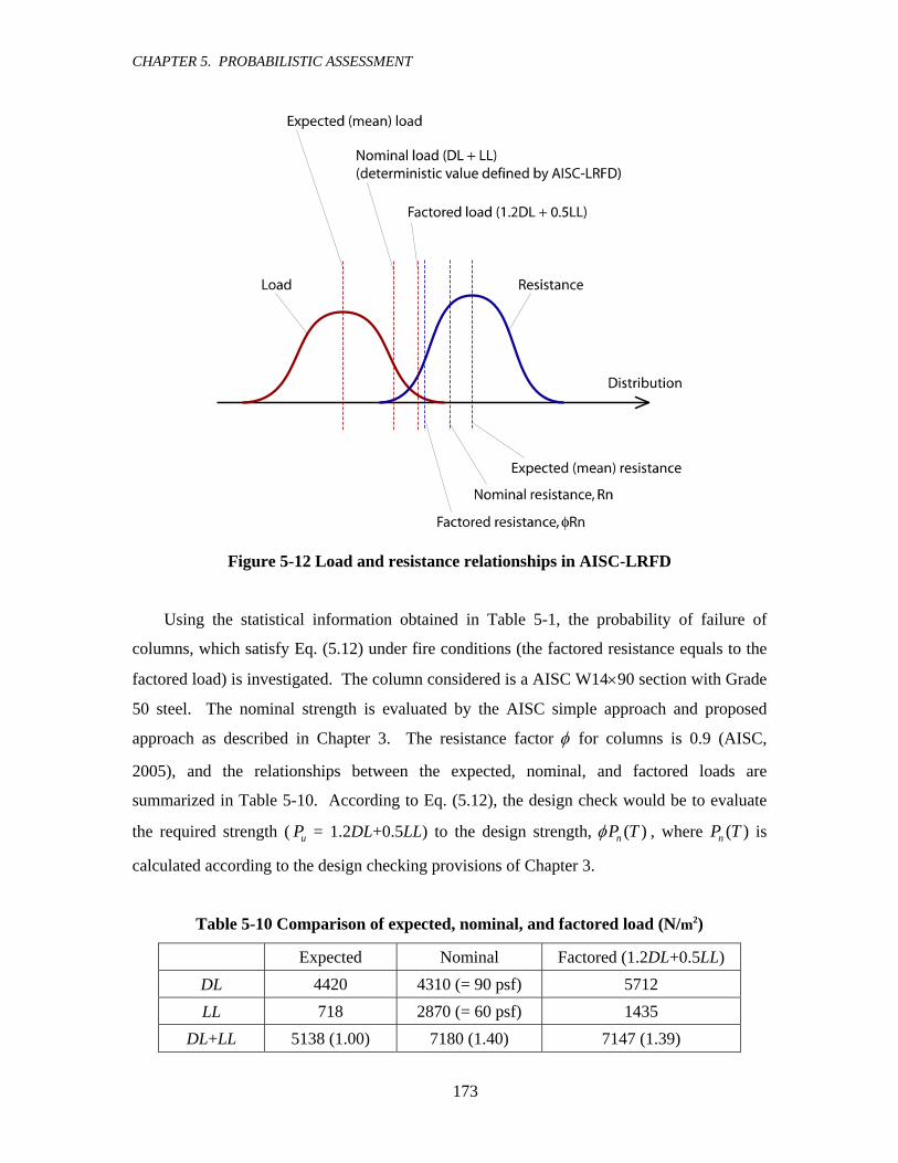
CHAPTER 5. PROBABILISTIC ASSESSMENT
173
Figure 5-12 Load and resistance relationships in AISC-LRFD
Using the statistical information obtained in Table 5-1, the probability of failure of
columns, which satisfy Eq. (5.12) under fire conditions (the factored resistance equals to the
factored load) is investigated. The column considered is a AISC W14×90 section with Grade
50 steel. The nominal strength is evaluated by the AISC simple approach and proposed
approach as described in Chapter 3. The resistance factor φ for columns is 0.9 (AISC,
2005), and the relationships between the expected, nominal, and factored loads are
summarized in Table 5-10. According to Eq. (5.12), the design check would be to evaluate
the required strength ( uP = 1.2DL+0.5LL) to the design strength, ( )nP Tφ , where ( )nP T is
calculated according to the design checking provisions of Chapter 3.
Table 5-10 Comparison of expected, nominal, and factored load (N/m2)
Expected Nominal Factored (1.2DL+0.5LL) DL 4420 4310 (= 90 psf) 5712 LL 718 2870 (= 60 psf) 1435
DL+LL 5138 (1.00) 7180 (1.40) 7147 (1.39)

CHAPTER 5. PROBABILISTIC ASSESSMENT
174
The relationships between the expected and nominal load are based on a past study
(Ellingwood, 1983) and the load factors for the dead and live load are defined in AISC
(2005). The ratio of the factored load (combined dead and live load) to the expected (mean)
load is 1.39. This ratio is assumed to be constant in this study.
The probability of failure of the columns under a specified constant elevated temperature
of 500 °C is assessed by using the mean-value first-order second-moment (FOSM) method
by the following procedure: (1) evaluate the nominal strength of the column by the AISC
simple approach, using both the AISC nominal strength equations and the proposed strength
equations (Chapter 3), (2) calculate the factored load such that Eq. (5.12) is satisfied, (3)
define the expected load as 1.00/1.39 of the factored load, and (4) evaluate the probability
that the load is greater than the resistance by FOSM. The purpose of this study is twofold:
(1) to confirm the accuracy of the design equations (AISC and proposed) and (2) to
investigate the effect of uncertainties. Dead and live loads are the random variables for the
load distribution, and the yield strength and elastic modulus of steel at elevated temperatures
( ( )yF T and ( )E T ) are considered as the random variables for the resistance distribution.
The statistical information (mean and c.o.v.) of these random variables is shown in Table 5-1.
FEM simulations are performed for the evaluation of the gradient of the resistance with
respect to the random variables. Details of the modeling are described in Chapter 3.
The probability of failure of W14×90 columns with varied member length is shown in
Figure 5-13. Two sets of data are shown in the figure. One is for cases where the nominal
strength is calculated by the AISC approach, and the other is for cases where the proposed
strength equations are used. Figure 5-13(a) shows the beta function (the definition is shown
in Appendix B.4) and Figure 5-13(b) shows the probability of failure (these figures have a
complementary relationship). As described in Chapter 3, the nominal strength equations of
AISC are known to be unconservative, especially for columns with intermediate length
(slenderness ratio of 40-100). The results from this study are consistent with those from
Chapter 3, where referring to Figure 5-13(b), the probability of failure with the slenderness
ratio of 60 is about 37 %.
In terms of accuracy, deterministic studied are performed for different temperatures,
section sizes, and steel strength in Chapter 3 and the accuracy of the proposed equations are
confirmed. In order to investigate the effect of uncertainty, this case study represents other
cases with different section sizes and steel strength, because the statistical properties of the

CHAPTER 5. PROBABILISTIC ASSESSMENT
175
uncertainties are not functions of temperatures and constantly defined regardless section sizes
and steel strength.
0 50 100 150 2000
0.5
1
1.5
2
2.5
3
L / ry
β
AISCProposed
0 50 100 150 2000
0.1
0.2
0.3
0.4
L / ry
P (f
ailu
re)
AISCProposed
(a) β (b) Probability of failure
Figure 5-13 Probability of failure of W14×90 column at 500 °C with varied length
The probability of failure shown in Figure 5-13 is calculated assuming that the resistance
factor φ = 0.9. Alternatively, required φ values for the target probabilities of failure at 500
°C can be evaluated. Assuming a target probability of 0.47 % (β = 2.6) as the AISC
commentary indicates for members at ambient temperature, the required φ values are shown
in Figure 5-14. The required φ factors would need to be about 0.5 to 0.7 for the AISC
equations and 0.7 to 0.9 using the proposed member strength provisions.
0 50 100 150 2000
0.2
0.4
0.6
0.8
1
L / ry
φ
AISCProposed
Figure 5-14 φ factors for 0.47 % (β = 2.6) probability of failure of W14×90 column at
500 °C with varied length

CHAPTER 5. PROBABILISTIC ASSESSMENT
176
A similar study is performed for the column with a fixed length of 4 m (this gives a
slenderness ratio of 42.3 about the weak axis) with varied elevated temperatures up to 800
°C. The probability of failure is shown in Figure 5-15. A large probability of failure (about
30 %) is observed for the column design based on the AISC approach at elevated
temperatures greater than 400 °C, whereas the probability of failure based on the proposed
approach is less than 3 % and varies less with respect to temperature.
0 200 400 600 8000
0.5
1
1.5
2
2.5
3
3.5
Temperature (°C)
β
AISCProposed
0 200 400 600 8000
0.1
0.2
0.3
0.4
Temperature (°C)
P (f
ailu
re)
AISCProposed
(a) β (b) Probability of failure
Figure 5-15 Probability of failure of W14×90 (L = 4 m) column with varied temperatures
Required φ values for the 0.47 % (β = 2.6) target probability of failure are also
investigated with the fixed length (4 m) column at elevated temperatures. The values for the
column based on the AISC approach are about 0.5 at elevated temperatures greater than 400
°C, while those based on the proposed approach are about 0.7.
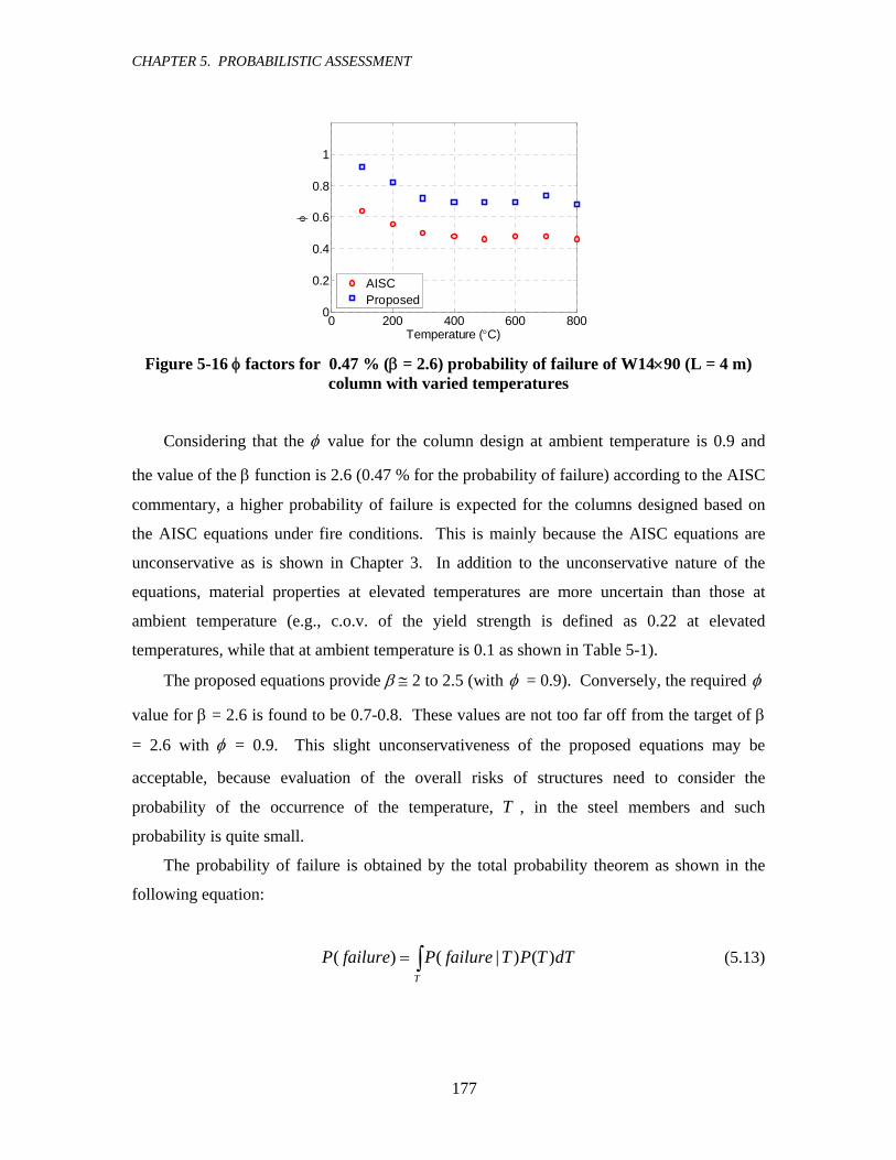
CHAPTER 5. PROBABILISTIC ASSESSMENT
177
0 200 400 600 8000
0.2
0.4
0.6
0.8
1
Temperature (°C)
φAISCProposed
Figure 5-16 φ factors for 0.47 % (β = 2.6) probability of failure of W14×90 (L = 4 m)
column with varied temperatures
Considering that the φ value for the column design at ambient temperature is 0.9 and
the value of the β function is 2.6 (0.47 % for the probability of failure) according to the AISC
commentary, a higher probability of failure is expected for the columns designed based on
the AISC equations under fire conditions. This is mainly because the AISC equations are
unconservative as is shown in Chapter 3. In addition to the unconservative nature of the
equations, material properties at elevated temperatures are more uncertain than those at
ambient temperature (e.g., c.o.v. of the yield strength is defined as 0.22 at elevated
temperatures, while that at ambient temperature is 0.1 as shown in Table 5-1).
The proposed equations provide β ≅ 2 to 2.5 (with φ = 0.9). Conversely, the required φ
value for β = 2.6 is found to be 0.7-0.8. These values are not too far off from the target of β
= 2.6 with φ = 0.9. This slight unconservativeness of the proposed equations may be
acceptable, because evaluation of the overall risks of structures need to consider the
probability of the occurrence of the temperature, T , in the steel members and such
probability is quite small.
The probability of failure is obtained by the total probability theorem as shown in the
following equation:
( ) ( | ) ( )T
P failure P failure T P T dT= ∫ (5.13)
CHAPTER 5. PROBABILISTIC ASSESSMENT
178
where ( | )P failure T is the probability of failure at a given elevated temperature and ( )P T
is the probability of the occurrence of T in the steel members. ( )P T is also evaluated
considering the probability of the temperature of the steel members reaching T under
flashover fires, ( | )P T flashover fire , and the probability of flashover fires,
( )P flashover fire , during a certain time, i.e., mean annual probability of flashover fires.
Similar to Eq. (5.13), ( )P T can be obtained by using the total probability theorem,
integrating ( | )P T flashover fire and ( )P flashover fire over time t .
( ) ( | ) ( )t
P T P T flashover fire P flashover fire dt= ∫ (5.14)
This brief overview of the overall risk assessment of steel structures against fires
provides some ideas about the issues of structural risk assessment for fires. This research
focuses on the structural aspects. Future coordination with other aspects of risk assessment
against fires is still needed.
5.3.4 Conclusions
Conclusions obtained in this chapter are summarized in the following points:
1. Statistical properties (mean and coefficient of variation) of uncertain structural variables
are defined by reviewing past test data and studies, as well as by using engineering
judgment for those factors whose statistical information is unknown. The uncertain
variables are dead and live loads, yield strength and elastic modulus of steel at elevated
temperatures, strength and deformation capacity of bolted connections, and the
longitudinal constraint spring properties. The coefficient of variation of the yield
strength of the steel and the shear strength of bolts are defined as 0.22 and 0.29,
respectively, based on existing test data. Statistical properties of the loads are assumed
to be the same as those at ambient temperature. The properties of the elastic modulus of
steel and other variables are approximately defined using engineering judgment.
2. The variation of the time-temperature relationships is investigated by applying various
values to fuel load, firefighting factor, and opening factor. These are used in the
parametric fire curve defined in Eurocode 1 (2002). The maximum temperature of
insulated steel members can vary from 340 °C to 1000 °C and those of unprotected

CHAPTER 5. PROBABILISTIC ASSESSMENT
179
members can be 780-1300 °C. These highly varied maximum steel temperatures are the
consequence of the uncertain fire behavior that controls structural stability. Further
research and development is needed to integrate the fire and structural simulations in a
unified probabilistic assessment.
3. The sensitivity of the critical temperatures of three sub-assembly structures (interior
column, beam, and exterior column) is evaluated for the uncertain variables. Yield
strength of steel is the most influential factor for the interior column, because the
slenderness ratio of the column is relatively small and the limit-state mechanism is
inelastic buckling, which is controlled by material strength. For the beam sub-assembly,
the deformation capacity of the bolted connections is the most influential factor. This
implies that axial force induced by the thermal expansion overwhelms the strength of the
bolted connections, and strengthening connections is less effective at preventing the
connection failure than enhancing the deformation capacity of the connection. For the
exterior beam-column sub-assembly, the strength of the bolted connection is the most
influential parameter. This is because the connection fails due to the tensile axial force
induced in the beam by catenary action.
4. The magnitude of the gas temperature during the compartment fire is scaled and the
probability of collapse with respect to the given gas temperature is assessed for the three
sub-assemblies, using the mean-value first-order second-moment (FOSM) method. The
interior column is studied with and without fire insulation. The mean gas temperature
for the limit-states significantly increases from 616 °C to 1399 °C with the fire
insulation. The mean gas temperature for the un-insulated beam sub-assembly is 604 °C
due to the connection failure. Furthermore, the variability of the failure point of the
beam sub-assembly is greater than that of the interior column sub-assembly (i.e., greater
uncertainty in the beam sub-assembly). Conversely, relatively smaller variability is
observed in the exterior column sub-assembly (with insulated column and un-insulated
beam), where the mean gas temperature for the limit-state is 763 °C. Of the three sub-
assemblies, the interior column sub-assembly without insulation is the most critical.
This assessment shows that the failure of the beam sub-assembly can be the dominating
mechanism (probability of interior column buckling at 620 °C is about 50 %, while that
of the connection failure of the beam at the temperature is about 25 %); however failure
of the exterior column sub-assembly would almost never control.

CHAPTER 5. PROBABILISTIC ASSESSMENT
180
5. The probability of failure of the columns under a given elevated temperature is evaluated
for columns designed using the AISC-LRFD simple method (2005 specification) and the
proposed equations in Chapter 3. The uncertain variables are dead and live load, and
yield strength and elastic modulus of steel at elevated temperatures. The evaluation is
performed using the mean-value FOSM method for a W14×90 column (Grade 50) with
varied member length or temperature. The maximum probability of failure at elevated
temperature is about 40 % for the columns based on the AISC design strength equations,
while it is 3-4 % for the columns based on the proposed design strength equations.
Consistent results (high unconservativeness for columns with intermediate length) are
observed for the AISC method as discussed in Chapter 3. Required values for the
resistance factor to satisfy 0.47 % (β = 2.6) probability of failure given elevated
temperatures are evaluated. The values are 0.5-0.7 and 0.7-0.9 for the design based on
the AISC and proposed equations, respectively. This slight unconservativeness of the
proposed equations may be acceptable, because evaluation of the overall risks of
structures need to consider the probability of the occurrence of the temperature in the
steel members and such probability is quite small.

181
CHAPTER 6 CONCLUSIONS
6 CONCLUSIONS
6.1 GENERAL
The main objective of this research is to investigate the collapse performance of steel-framed
buildings under fully developed (flashover) fires. This research approach employs detailed
finite element simulations to assess the strength of individual members (beams and columns)
and indeterminate structural sub-assemblies (beams, columns, connections and floor
diaphragms). One specific focus of the investigation is to assess the accuracy of beam and
column strength design equations of the Eurocode 3 (2003) and the American Institute of
Steel Construction (AISC) Specification (2005). An outcome of the structural member study
is a proposal for alternate equations to improve the accuracy of the AISC Specification
provisions.
To examine the collapse limit-state response of building systems, structural sub-
assemblies are devised to examine indeterminate effects of gravity-framing systems,
including forces induced by restraint to thermal expansion and nonlinear force redistribution
due to yielding and large deformations. The sub-assemblies are based on gravity framing for
an archetypical mid-rise office building, with structural steel framing details that are
representative of design and construction practice in the United States. These studies identify
the governing factors in structural system collapse, including the effectiveness of fire
insulation or alternate techniques (e.g., strengthening of connections) to increase the collapse
resistance.
The significance of uncertainties in gravity loading and structural parameters on collapse
due to fire are investigated through a probabilistic assessment that includes statistical
characterization of key parameters and the mean-value first-order second-moment (FOSM)
analyses to integrate their effects. At the individual component level, the reliability of the
current AISC Specification and proposed alternative design equations are evaluated.

CHAPTER 6. CONCLUSIONS
182
Reliability studies of the sub-assembly models are conducted to assess conditional
probabilities of collapse in gravity framing systems for a specified elevated temperature.
In this chapter, the notable findings from this research are highlighted and summarized.
6.2 SUMMARY
6.2.1 Steel Properties at Elevated Temperatures
Existing test data of structural steel properties (stress-strain curves) at elevated temperatures,
reported by five research groups (Harmathy and Stanzak, 1970; Skinner, 1972; DeFalco,
1974; Fujimoto et al.,1980, 1981; Kirby and Preston, 1988), are reviewed and compared with
design equations in four specifications: Eurocode (European countries), AS4100 (Australia),
AISC (the US) and AIJ (Japan) in Chapter 2. The measured stress-strain curves are
normalized with respect to the measured 0.2 % off-set strength at ambient temperature, and
reduction ratios of the strength at elevated temperatures are evaluated. The test data clearly
show that the stress-strain curves at elevated temperatures experience early non-linearity
(deterioration of the tangent stiffness) below the yield point, which is distinctly different from
the characteristic elastic-plastic behavior of steel at ambient temperatures. This behavior is in
contrast to the elevated temperature provisions of the AS4100 and AISC standards, where the
specified degradation parameters imply use of the same characteristic elastic-plastic stress-
strain response at both ambient and elevated temperatures. Consequently, the implied
elevated temperature stress-strain curves do not fit the experimental data well. The AIJ
provisions define non-linear curves incorporating deterioration of the tangent stiffness;
however, the curves are conservatively defined by including large safety margins in the
material properties. The design equations by Eurocode are the most representative of the
experimental data.
Based on comparisons of measured data and proposed stress-strain models, the stress-
strain equations of steel response at elevated temperatures defined by Eurocode are adopted
in this research for analytical simulations. Statistical data to describe the variability in steel
strength deterioration ratios at elevated temperatures are also obtained and used in and the
probabilistic studies, reported in Chapter 5.

CHAPTER 6. CONCLUSIONS
183
6.2.2 Past Fire Disasters
Past fire disasters on steel buildings are reviewed in Chapter 2 to investigate the observed
collapse behavior of actual steel buildings subjected to fires. Four major fire events:
Broadgate Phase 8, One Meridian Plaza, the World Trade Center (WTC) building 7 and the
Windsor Building, as well as the Cardington eight-story full-scale fire test are reviewed in
detail. The most important finding from this review is that no steel building has totally
collapsed from fire except the WTC 7 building, which had some unique circumstances (a
non-redundant transfer truss system and possibly damaged caused by falling debris from the
WTC 1 tower). These observations demonstrate the potential strength of steel buildings
designed as per current practice against fires. The superior fire resisting ability of steel
beams was clearly observed in the Broadgate Phase 8, One Meridian Plaza and the
Cardington Fire Test, where insulation was not present on the beams. Some of the beams in
these structures experienced temperatures greater than 1000 °C and deformed considerably;
however, they did not collapse. In contrast, the vulnerability of steel columns to fire was
clearly observed. The Windsor Building partially collapsed in the upper stories where fire
insulation on the columns was missing due to renovation. Also, local buckling on columns
with significant distortion, which greatly deteriorated the vertical load carrying capacity of
the columns, was observed in the Cardington Fire Test. These observations are useful for
understanding the characteristic behavior of steel buildings under fires, although further
careful investigations are necessary to generalize the findings for structural fire design.
6.2.3 Member-based Strength Study
The individual member strengths of I-shaped steel columns and beams are studied using
detailed three-dimensional finite shell element models, where the strengths under specified
elevated temperatures are parametrically investigated. Residual stress and geometric
imperfections are taken into account in the simulations; and the analytical simulations are
validated by comparison to existing test data for columns. In column models subjected to
axial force, flexural buckling is found to be the critical mechanism. Beam models capable of
simulating non-uniform torsion are subjected to uniformly-distributed moment about the
strong-axis, and lateral torsional buckling as well as yielding are the critical mechanisms.
Accuracy of the member-based design criteria defined in Eurocode is confirmed through
comparison with the simulation data, while the AISC criteria is found to be highly

CHAPTER 6. CONCLUSIONS
184
unconservative. Alternative design equations for AISC are proposed for I-shaped steel
columns, unbraced beams, and beam-columns at elevated temperatures.
6.2.4 Benchmark Building Study
The performance of gravity framing in steel-framed office buildings under localized fires is
assessed through study of an archetypical building design in Chapter 4. The plan of the ten
story building is 32.0 m by 25.6 m and a localized fire is assumed to break out on the second
floor. Four possible failure mechanisms (i.e., interior column buckling, exterior column
buckling, beam yielding and interactive failure, where beam deformation in the fire
compartment causes multi-story exterior column buckling) are simulated with sub-assembly
analysis models. Beam and columns in the sub-assembly models are composed of shell finite
elements; and nonlinear springs are used to model connections and boundary conditions
imposed by the surrounding structure. Non-linear spring properties are based on
supplemental models that take into account the effects of the concrete floor slab and the
behavior of the bolted connections. The critical failure mechanisms and temperatures are
investigated, and design recommendations to improve the collapse capacity are suggested.
6.2.5 Probabilistic Studies
Assessment of structural collapse due to fire involves large uncertainties in fire development,
heat transfer, and structural behavior. Fire development is highly uncertain and depends on
various factors such as fuel load, geometry of the fire compartments, and firefighting
activities. Additionally, heat transfer into the structural steel involves uncertainties in
compartment gas temperatures, radiation effects, and effectiveness of thermal insulation.
While the importance of these two factors (fire development and heat transfer) is recognized,
detailed study of them is outside the scope of this study. Rather, the probabilistic aspect of
this research focuses on uncertainties in the structural gravity loading and response aspects
under elevated temperatures. Statistical information (i.e., mean and coefficient of variation)
of characteristic structural factors (e.g., steel properties at elevated temperatures) are
investigated. Using the statistical information, the sensitivities of the collapse limit-state of
both individual steel members and structural sub-assemblies under the localized fire with
respect to the uncertain factors are evaluated. Specifically, the collapse probabilities of the
structural sub-assemblies are evaluated using the mean-value FOSM approach for given gas
CHAPTER 6. CONCLUSIONS
185
temperatures in the fire compartment. Reliability aspects of the AISC design equations for
columns are included in the study.
6.3 MAJOR FINDINGS AND CONCLUSIONS
The main findings and general conclusions obtained from this research are summarized in the
following sections.
6.3.1 AISC Member-based Design Criteria
The AISC Specification’s (2005) new provisions for assessment of the design strength of
members at elevated temperatures are based on the standard design equations at ambient
temperatures, where the input material properties (elastic stiffness and yield strength) are
reduced using the material degradation factors defined in the Eurocode (2003). Therefore, it
can be interpreted that the AISC method assumes use of the same elastic-plastic stress-strain
relationships for steel at elevated and ambient temperatures. This is in contrast to the actual
nonlinear stress-strain relationships, as shown in Chapter 2. For stability sensitive members,
errors arise because of the nonlinear deterioration of tangent stiffness below the nominal
yield point. Finite element simulations are performed for columns, unbraced beams and
beam-columns under parametrically changed elevated temperatures and member length. The
simulation results show that the AISC provisions are unconservative by up to 60 % for the
columns and 80-100 % for the beams and beam-columns. This unconservative behavior is
typically observed for members with intermediate length (slenderness ratio of 60-80), where
inelastic buckling is the critical failure mechanism. Member-based critical strengths
investigated by applying the tangent modulus theory (Appendix A), with the reduced
stiffness, agree well with the simulation data. The study shows explicit relationships between
material deterioration of the tangent stiffness and member strengths at elevated temperatures.
6.3.2 Effect of Residual Stress and Local Buckling
Three-dimensional finite shell element models, used in the simulations, are well-suited for
investigation of residual stress and local buckling. The maximum residual stress is assumed
as 20 % of the yield strength for members with Grade 50 steel, such that it deteriorates in
proportion to the degraded yield strength at elevated temperatures. The maximum difference
of the critical strength with and without consideration of the residual stress is less than 15 %,

CHAPTER 6. CONCLUSIONS
186
which is found for members with intermediate length (slenderness ratio of 100) at around 500
°C. Overall, the order of magnitude of the effect of residual stresses is comparable at
ambient and elevated temperatures.
Local buckling is not critical for compact or near-compact sections at ambient
temperature. It is shown in this research that local buckling is similarly not critical for
compact and near-compact members at elevated temperatures. Local buckling is observed in
the post-buckling stage, but it does not control the critical strength. The only exception to
this was observed for a very short segment of a non-compact W14×22 column, where the
strength was limited by local buckling at a stress approximately equal to 60 % of the yield
strength at elevated temperatures. This extreme case study is purposely carried out to verify
that local buckling is not a major concern for compact sections at elevated temperatures
relative to ambient temperature.
6.3.3 Proposed Design Criteria for AISC
Motivated by the unconservativeness of the AISC member design equations, alternative
design equations for steel columns and beams at elevated temperatures are proposed. These
equations are functions of temperature and member length, and follow a similar format to the
existing AISC design equations at ambient temperature. The accuracy of these equations is
validated with the analytical simulations under various specified elevated temperatures and
member lengths. The strengths calculated by the proposed equations are within 20-30 % of
the strengths calculated by finite element simulations. This agreement is comparable to that
observed between Eurocode equations and simulations (10-20 %). More than eight hundred
simulations are performed in total to verify the proposed equations, accompanied by studies
on members with different steel strengths and section sizes.
6.3.4 Steel-framed Building under Localized Fire
In simulations of the steel-framed benchmark building under localized fires, the members are
initially assumed to be bare (un-insulated). In this case, the governing failure mechanism is
interior column buckling at a critical column temperature of 578 °C (gas temperature of 920
°C). Assuming insulation on the columns (with no insulation on the beams) increases the
critical gas temperature to 965 °C. The second critical failure mode occurs for the interior
(secondary) beams, which experience failure of the bolted shear-tab connection at a critical

CHAPTER 6. CONCLUSIONS
187
beam temperature of 634 °C in the lower flange. This failure is caused by thermal expansion
which induces large axial forces in the beams and the bolted connections. Typical shear-tab
connections are designed for beam shear force due to gravity and failure of this type of
connections is critical for beams under fires. Design improvements of these bolted shear-tab
connections for interior beams are proposed (discussed later at 6.4.1 Design
Recommendations), which can increase the critical temperature for interior beams. The third
critical failure mode occurs through an interactive mechanism between the exterior column
and the beam which provided out of plane support to the column. For this limit-state, the
temperatures at the exterior column and lower flange of the beam are 145 °C and 812 °C,
respectively (low column temperature in the column because of the insulation).
Using fire insulation is the only practical solution to prevent column buckling, because
using a larger steel section as an alternative design approach is economically infeasible;
however, bolted connection failure for beams can be prevented without fire insulation. Using
slotted bolt holes or placing steel reinforcement in the composite concrete slab can
significantly improve the performance of the connections under fires by releasing additional
shear force or bracing longitudinal strength of the connections. Where connections are
appropriately reinforced, steel beams have potentially high load carrying capacity with
catenary action that can develop under large sagging deformations. Assuming that this large
deformation is allowed, fire insulation for beams can be reduced or even eliminated by
improving the connections.
6.3.5 Longitudinal Constraint of Interior Column
Building columns that expand during a fire may be subjected to high axial compression
loads, depending on the constraint stiffness provided by framing levels above the heated
column. Typical bolted shear-tab connections, which are used at connections between
columns and gravity floor beams, are often considered as having negligible rotational
stiffness. This assumption significantly simplifies design calculations and is usually
conservative; however, this assumption is not necessarily conservative when the rotational
stiffness provides vertical constraint that can induce axial compression forces in a heated
column. To investigate this effect, the rotational stiffness of typical shear-tab connections is
evaluated based on tests by Liu and Astaneh-Asl (2004). Results calculated for three building
heights (5, 10 and 20 stories) with a fire at the second floor, indicate that the axial forces

CHAPTER 6. CONCLUSIONS
188
induced by vertical restraint have a negligible effect (less than 1 % change in critical column
temperature) on the column axial strength. The reason for this is that the column loses both
stiffness and yield strength as it elongates with increasing temperature. Therefore, while
constraint to the thermal elongation alone may induce large axial compressions, when
combined with the associated material degradation the induced forces are negligible.
6.3.6 Longitudinal Constraint of Beam
Floor framing that surrounds the beams subjected to a compartment fire can provide
significant constraint to longitudinal deformation of the heated floor beams. This constraint
has beneficial and negative effects. The negative effect is that the restraint to beam
elongation during the heating phase of response can lead to premature failure, such as bolt
shear (as described previously). Provided steps are taken to avoid premature failure modes,
the constraint can enable catenary action that can greatly increase the gravity load resistance
at elevated temperatures. Studies of interior beams showed that where constraint is provided
by the surrounding framing, the critical temperature increased from 634 °C to 812 °C.
However, typical beam connections are not strong enough to support the catenary action and
connection design enhancements are needed to achieve this improved performance.
Evaluation of the longitudinal constraint of beams is difficult, however, and involves
many complex issues such as non-linear behavior of the concrete slab, the stud connections
between steel beams and concrete slab, steel connections, and 3D effects from the stiffness of
vertical components including the lateral resisting system. Relatively simple analyses are
carried out for this evaluation using elastic FEM models for the floor structure. Although
evaluation of the longitudinal constraint stiffness of beams is approximated, a sensitivity
study shows that accuracy of the stiffness is not critical to overall beam behavior under fire
conditions.
6.3.7 Properties of Bolted Connections
Since failure of bolted connections is critical in some failure mechanisms, realistic evaluation
and modeling of the bolted connections are essential for this research. The strength reduction
ratio of bolts defined in ECCS (2001) is compared with existing test data by Kirby (1995)
and Yu (2006). The ECCS reduction ratio agrees well with the test data within 20-30 % up to
700 °C. Bilinear force-displacement relationships including post capping softening is
assumed for longitudinal springs of shear-tab type bolted connections for beam sub-assembly

CHAPTER 6. CONCLUSIONS
189
analysis models. The simulation results show that compressive axial force of the beams due
to thermal elongation causes the bolted connection failure. In order to prevent this failure,
slotted bolt holes are suggested as a design improvement and its effectiveness is validated in
simulations.
6.3.8 Evaluation of Structural Uncertainties
The characteristic parameters needed for the structural fire simulations are reviewed for their
statistical properties. These factors are the dead load, live load, yield strength and elastic
modulus of steel at elevated temperatures, strength (force-displacement relationship) of the
vertical constraint spring for the interior column, longitudinal constraint stiffness for the
beams, and shear strength and deformation capacity of bolted connections. In particular, the
statistical properties of the steel strength at elevated temperatures are carefully investigated
by reviewing past experimental data, and the coefficient of variation is determined to be 0.22.
Investigations of the effect of these uncertainties indicate that the strength limit-states are
most sensitive to the degraded yield strength of steel at elevated temperatures. Also, the
limit-state of the beams that fail due to thermal elongation is sensitive to the deformation
capacity of bolted connections.
6.3.9 Probabilistic Studies
Using the statistical information on the variability in structural parameters, the collapse
probabilities of the sub-assemblies in the benchmark building are evaluated as a function of
gas temperatures in the localized compartment fire. The evaluation is performed by the
mean-value (FOSM) approach. Assuming deterministic relationships between the steel and
gas temperatures in the fire compartment (which are obtained through the incremental time
step simulation), the probability of failure of the three sub-assembly models is evaluated with
respect to the gas temperature.
The magnitude of the gas temperature during the compartment fire is scaled and the
probability of collapse with respect to the given gas temperature is assessed for the three sub-
assemblies. No fire insulation is assumed for the steel members except for the exterior
column. Among the three sub-assemblies, the largest variability is observed for the beam
sub-assembly. The critical collapse mechanism is buckling of the interior column. This
assessment shows that the connection failure of the beam sub-assembly is also a significant
mechanism, since the probability of interior column buckling at 620 °C is about 50 %, while

CHAPTER 6. CONCLUSIONS
190
that of the connection failure of the beam at the temperature is about 25 %. Failure of the
exterior column sub-assembly would almost never control over the interior column and beam
mechanisms.
The probability of failure of columns given elevated temperatures is evaluated for those
designed based on the AISC-LRFD simple method (2005 specification) and the proposed
equations. The uncertain variables are dead and live load, and yield strength and elastic
modulus of steel at elevated temperatures. The evaluation is performed by using the mean-
value FOSM method for AISC W14×90 I-shaped columns (Grade 50) with varying member
length or temperatures. The probability of column failure ranges from 4 % to 38 % (β = 0.3-
1.8) for designs based on the AISC strength provisions (with φ = 0.9). These probabilities
reduce to 0.5 % to 3 % (β = 1.9-2.6) based on the proposed equations (with φ = 0.9).
6.4 DESIGN AND ANALYTICAL MODELING RECOMMENDATIONS
6.4.1 Design Recommendations
In the review of the past fire disasters and the Cardington fire test in Chapter 2, it is reported
that some of the steel buildings did not collapse under fires without insulations. This fact
shows the potential strength of steel buildings against fires and questions the rationale of
current structural fire engineering practice. Three interesting points are found through the
simulations of the benchmark building in this research: (1) buckling of un-insulated gravity
columns are inevitable under flashover fires, making fire insulation on columns necessary to
prevent collapse, (2) beams can maintain their gravity load carrying ability at elevated
temperatures associated with large deformation, (3) failure of typical shear-tab bolted
connections is critical for the beams. One design recommendation derived from these
findings is to brace or protect connections for axial strength of beams at high temperatures.
Consequently, fire insulation on beams can be reduced or eliminated. The benefit of the
reduction or elimination of the beam insulation can have both economical and environmental
advantages. In terms of economics, conventional fire insulation has been reported to
contribute up to 30 % of bare steel costs for steel buildings (Lawson, 2001). Therefore, the
resulting savings by using less insulation could be applied to improve other fire protection
systems (e.g., egress). From an environmental (indoor air quality standpoint), spray type fire
insulation, which is commonly employed for beam insulation, is considered to be

CHAPTER 6. CONCLUSIONS
191
environmentally unfriendly. Therefore, removal or minimization of beam insulation (which
is more prone to dislodging and getting into the air) is desirable. By bracing the connections
against fires, steel structures will be more redundant and thus preventing progressive
collapse. On the other hand, large deformation of the beams under fires may not be
acceptable in some cases such as possible break of the fire partitions, prevention of smooth
evacuation, and difficulty in post-fire renovation. The recommendation must be further
studied with discussion on quantitative evaluation on improvement of structural performance
as well as risk, environmental, and economical assessment.
6.4.2 Analytical Modeling Recommendations
The advantage to using shell element models for I-shaped steel sections is its capability to
simulate local buckling. It is observed in this research that local buckling is significant to the
post-buckling strength and limit-state strength of non-compact sections. In order to study
these issues, shell element models are used in this research; however, using fiber element
models would lead to the same results if the research focuses on only the member-based
limit-state strength study for compact sections. Post-buckling strength of columns is an
important factor for study of indeterminate systems related to progressive collapse under fires
and shell element models are recommended for this purpose. Beam behavior is controlled
less by local buckling and fiber models can work well for beams. Using hybrid shell and fiber
models for columns and beams is a possible option for frame studies to reduce computational
time.
Although the proposed sub-assembly models are concise and efficient to simulate
accurately the characteristic behavior of building frames under fires, even simpler models are
preferred for practical use. For this purpose, two modeling improvements that are worth
investigation are modeling of bolted connections and the concrete floor slab. Development
of lumped spring models for bolted connections, which can simulate behavior under
combined axial, shear and moment at elevated temperatures, could drastically simplify
simulations. This effort should be carried out through calibration with test data. Modeling of
the concrete slab is a difficult aspect in structural fire simulations. However, approximate
modeling of the concrete slab is acceptable for practical purpose, since structural behavior is
shown in this research not to be sensitive to the stiffness. Using membrane elements instead
of shell elements for the concrete slab is another possible alternative. In both modeling
methods, analytical convergence would be a critical problem due to physical softening

CHAPTER 6. CONCLUSIONS
192
behavior of bolted connections and concrete slabs. An efficient analytical algorithm needs to
be developed for this goal.
6.5 FUTURE WORK
6.5.1 Member-based Strength Evaluation
Although this research on the critical strength of individual steel members provides useful
information for improvement of current structural fire design specification, there are many
areas that need to be developed in future research. Current research focuses on bi-symmetric
I-shaped members with compact (or near-compact) sections assuming a uniform temperature
distribution through the member cross section. In order to provide thoroughly a useful
simple individual member design approach under fire conditions, studies on non-symmetric,
non-compact sections are needed. A non-uniform temperature distribution along the member
length generally increases the critical strength; however, a non-uniform temperature
distribution in the section can be unconservative for slender members where induced
deformation deteriorates the member stability due to P-δ effects. The critical strength can
deteriorate by 50 % with a linear temperature distribution (ambient temperature at one edge
and elevated temperature at the other) and a slenderness ratio of 140 or greater. Also, the
assumption of a uniformly-distributed bending moment for beams and beam-columns is
useful for a prototype study; however, it must be extended to non-uniform moment for
generalization.
Reliability analysis of uncertainties, which is carried out in the performance evaluation
of frames, is in need of further study for individual member strength evaluation. It should
address a broader range of design and response parameters, including variations in cross-
section types, thermal and mechanical loading intensities and distributions, material
properties at ambient and elevated temperatures, and temperature induced distortions.
6.5.2 Performance Evaluation of Steel Buildings under Fires
A limit-state study of a benchmark steel building under a given localized fire scenario is
performed by finite element analyses introducing sub-assembly simulation models. Although
characteristic behaviors for an indeterminate structure such as post-buckling stability of
columns and catenary action of beams is evaluated, more case studies with different types of
steel buildings and various fire scenarios are needed for generalizing the findings. More

CHAPTER 6. CONCLUSIONS
193
simulations of alternative designs are also needed with different conditions in order to
confirm the effects and allow for practical application.

CHAPTER 6. CONCLUSIONS
194

195
APPENDIX A SUPPLEMENTAL STUDIES ON INDIVIDUAL MEMBERS
A SUPPLEMENTAL STUDIES ON INDIVIDUAL MEMBERS
A.1 TANGENT MODULUS THEORY
A.1.1 Flexural Buckling
Inelastic critical strength of ideally straight columns can be theoretically derived by tangent
modulus theory (TMT), which has been primarily studied in 1960’s, and these efforts are
described in previous literature (e.g., Galambos, 1998). According to the theory, the critical
strength is simply given by substituting tangent stiffness into elastic stiffness in the elastic
buckling equation.
2
00, 2
( )( / )
tcr tan
E APL r
π ε= (A.1)
where 0,cr tanP is the critical strength by tangent modulus theory. ε is a strain and uniform in
sections. 0 ( )tE ε is tangent stiffness under the stain ε . A, r and L are the cross-sectional
area, radius of gyration, and length, respectively.
Although the theory provides useful insight for column strength against inelastic
buckling, derived critical strengths do not necessarily agree well with test results due to lack
of consideration of imperfections. Geometric imperfections and deformed bent form
deteriorate the critical strength because of the P-δ effect. Also, residual stress causes non-
uniform strain and tangent stiffness in sections.
Using this theory and accepting some degree of inaccuracy, the tangent modulus theory
is applied to analyze column strength at elevated temperatures. Ideally straight steel columns
without residual stress are first considered. The critical strength under elevated temperatures
against flexural buckling is obtained by the tangent modulus theory as Eq. (A.2).
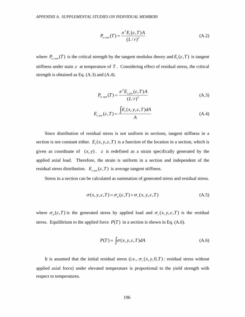
APPENDIX A. SUPPLEMENTAL STUDIES ON INDIVIDUAL MEMBERS
196
2
, 2
( , )( )( / )
tcr tan
E T AP TL r
π ε= (A.2)
where , ( )cr tanP T is the critical strength by the tangent modulus theory and ( , )tE Tε is tangent
stiffness under stain ε at temperature of T . Considering effect of residual stress, the critical
strength is obtained as Eq. (A.3) and (A.4).
2
,, 2
( , )( )
( )t ave
cr tan
E T AP T
L rπ ε
= (A.3)
,
( , , , )( , ) t
t ave
E x y T dAE T
A
εε = ∫ (A.4)
Since distribution of residual stress is not uniform in sections, tangent stiffness in a
section is not constant either. ( , , , )tE x y Tε is a function of the location in a section, which is
given as coordinate of ( , )x y . ε is redefined as a strain specifically generated by the
applied axial load. Therefore, the strain is uniform in a section and independent of the
residual stress distribution. , ( , )t aveE Tε is average tangent stiffness.
Stress in a section can be calculated as summation of generated stress and residual stress.
( , , , ) ( , ) ( , , , )a rx y T T x y Tσ ε σ ε σ ε= + (A.5)
where ( , )a Tσ ε is the generated stress by applied load and ( , , , )r x y Tσ ε is the residual
stress. Equilibrium to the applied force ( )P T in a section is shown in Eq. (A.6).
( ) ( , , , )P T x y T dAσ ε= ∫ (A.6)
It is assumed that the initial residual stress (i.e., ( , ,0, )r x y Tσ : residual stress without
applied axial force) under elevated temperature is proportional to the yield strength with
respect to temperatures.

APPENDIX A. SUPPLEMENTAL STUDIES ON INDIVIDUAL MEMBERS
197
( , ,0, ) ( ) ( , ,0, 20°C)r y rx y T K T x yσ σ= (A.7)
where ( )yK T is reduction factor of yield strength in EC3. The initial residual stress satisfies
equilibrium in a section as shown in Eq. (A.8).
( , ,0, ) 0r x y T dAσ =∫ (A.8)
Eq. (A.8) is generally not true under applied axial force, because the magnitude of
residual stress is dependent of the generated strain by the axial force (Figure A-1).
Figure A-1 Strain level and residual stress
Relationship between the slenderness ratio and the critical strength by tangent modulus
theory is obtained by substituting ( )P T in Eq. (A.6) into , ( )cr tanP T in Eq. (A.3), where the
slenderness ratio is defined as L r , a ratio of the length with respect to radius of gyration
about buckling axis. Since , ( )t aveE T and ( )P T are uniquely defined with respect to ε ,
relationship between slenderness ratio and the critical strength can be iteratively calculated
with a variable of ε . Adopting the stress-strain curves of steel at elevated temperature from
EC3 (2003), the calculated critical strength under elevated temperatures with and without
consideration of residual stress is shown in Figure A-2. The critical strength in the figure is
normalized with plastic axial strength ( ) ( )y yP T A Tσ= , where ( )y Tσ is yield strength of
steel at elevated temperatures.
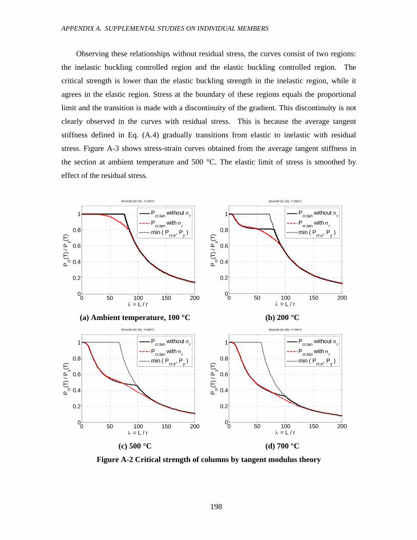
APPENDIX A. SUPPLEMENTAL STUDIES ON INDIVIDUAL MEMBERS
198
Observing these relationships without residual stress, the curves consist of two regions:
the inelastic buckling controlled region and the elastic buckling controlled region. The
critical strength is lower than the elastic buckling strength in the inelastic region, while it
agrees in the elastic region. Stress at the boundary of these regions equals the proportional
limit and the transition is made with a discontinuity of the gradient. This discontinuity is not
clearly observed in the curves with residual stress. This is because the average tangent
stiffness defined in Eq. (A.4) gradually transitions from elastic to inelastic with residual
stress. Figure A-3 shows stress-strain curves obtained from the average tangent stiffness in
the section at ambient temperature and 500 °C. The elastic limit of stress is smoothed by
effect of the residual stress.
0 50 100 150 2000
0.2
0.4
0.6
0.8
1
λ = L / r
Pcr
(T) /
Py(T
)
W14x90 (Gr.50), T=100°C
Pcr,tan without σr
Pcr,tan with σrmin ( Pcr,e, Py )
0 50 100 150 2000
0.2
0.4
0.6
0.8
1
λ = L / r
Pcr
(T) /
Py(T
)
W14x90 (Gr.50), T=200°C
Pcr,tan without σr
Pcr,tan with σrmin ( Pcr,e, Py )
(a) Ambient temperature, 100 °C (b) 200 °C
0 50 100 150 2000
0.2
0.4
0.6
0.8
1
λ = L / r
Pcr
(T) /
Py(T
)
W14x90 (Gr.50), T=500°C
Pcr,tan without σr
Pcr,tan with σrmin ( Pcr,e, Py )
0 50 100 150 2000
0.2
0.4
0.6
0.8
1
λ = L / r
Pcr
(T) /
Py(T
)
W14x90 (Gr.50), T=700°C
Pcr,tan without σr
Pcr,tan with σrmin ( Pcr,e, Py )
(c) 500 °C (d) 700 °C
Figure A-2 Critical strength of columns by tangent modulus theory

APPENDIX A. SUPPLEMENTAL STUDIES ON INDIVIDUAL MEMBERS
199
The difference of the critical strength with and without residual stress is most significant
around the discontinuous point. The location of the point increases in slenderness ratio with
higher temperature (e.g., L r = 75 is the location of the discontinuous point at ambient
temperature, while L r = 97 at 500 °C). Considering that the range of slenderness ratios
commonly used in practice is between 30 and 60 in building structures, it can be said that the
effect of residual stress for columns is less influential under elevated temperatures. It is also
noteworthy that the difference of the critical strength with and without residual stress
decreases under elevated temperatures (e.g., the difference is 14 % of ( )yF T at ambient
temperature, while it is 8 % at 500 °C).
Figure A-3 Stress-strain curves with the average tangent stiffness in section
Numerical analysis is carried out for a W14×90, which is a standard W-series section
issued by the American Institute of Steel Construction (AISC, 2005). This I-shaped section is
used as a prototype in this Appendix in both flexural and lateral torsional buckling studies.
The section is commonly used in practice for columns and its width-thickness ratio is greater
than most of the compact W-series sections in AISC. Therefore, the section is relatively
subjected to local buckling and a good model case to study strength against local buckling at
elevated temperatures.
The critical strength of columns against buckling about weak and strong axes at 500 °C
is calculated by FEM analysis with parametrically changed slenderness ratio (Figure A-4).

APPENDIX A. SUPPLEMENTAL STUDIES ON INDIVIDUAL MEMBERS
200
The figure superimposes the critical strength by the tangent modulus theory. The steel grade
is 50 ( 0yF = 345 MPa (50 ksi)) and the maximum residual stress is 69 MPa (10 ksi). Other
modeling assumptions are described in Chapter 3.
The greatest differences of the critical strength calculated with and without residual
stress are 1.8 % of ( )yP T for buckling about the strong axis and 4.3 % about the weak axis.
These maximum differences are observed when the slenderness ratio equals 100 for both
buckling strength about the strong and weak axes. This observation agrees with study results
of the tangent modulus theory. The critical strength computed by FEM analyses is lower
than that produced by the tangent modulus theory where the effect of residual stress is
significant. This is because additional stress generated by deformation at the limit state is
influential in this range of the slenderness ratio.
0 50 100 150 2000
0.2
0.4
0.6
0.8
1
L / r
Pcr
(T) /
Py(T
)
W14x90 Fy=345MPa T=500°C Strong Axis
Shell without σr
Shell with σr
TMT without σr
TMT with σr
0 50 100 150 2000
0.2
0.4
0.6
0.8
1
L / r
Pcr
(T) /
Py(T
)W14x90 Fy=345MPa T=500°C Weak Axis
Shell without σr
Shell with σr
TMT without σr
TMT with σr
(a) Buckling about strong axis (b) Buckling about weak axis
Figure A-4 The critical strength of W14×90 column
A.1.2 Lateral Torsional Buckling
The elastic critical bending moment of beams against lateral torsional buckling (LTB) under
constant bending moment about the strong axis is theoretically derived as Eq. (A.9)
(Timoshenko and Gere, 1961).
2
,cr e y y wEM EI GJ I C
L Lπ π⎛ ⎞= + ⎜ ⎟
⎝ ⎠ (A.9)

APPENDIX A. SUPPLEMENTAL STUDIES ON INDIVIDUAL MEMBERS
201
where yI , G , J , and wC are moment of inertia about weak axis, shear modulus, torsional
constant and warping constant, respectively. The first term in the square root in Eq. (A.9)
correspond to St. Venant torsion and the second term corresponds to warping torsion.
Studying a 4 m long W14×90 section, for instance, the second term is 440 % of the first term
and warping torsion dominates the overall elastic strength for LTB. In order to understand
behavior of lateral torsional buckling under elevated temperatures, tangent modulus theory is
again introduced to predict the critical moment for LTB, similar to the flexural buckling
study. Average tangent stiffness is approximately calculated by using simplified models with
two lumped sections as shown in Figure A-5. The area of each lumped section is equals to
half of the I-shaped section and, the distance between the lumped sections neth is defined
such that it satisfies the equation given in Eq. (A.10).
Figure A-5 Lumped fiber model
( ) ( )p yfM T P T h= (A.10)
where
( ) ( )p x yM T Z Tσ= (A.11)
( ) ( )yf f yP T A Tσ= (A.12)
where xZ is the plastic section modulus about the strong axis and fA is the area of a lumped
section. Without consideration of axial stress, strain of each lumped section is the same
magnitude and opposite sign. The absolute value of strain in the lumped section is defined as
ε and the corresponding curvature φ is given as 2 / nethε under the plane-section-remains-
plane assumption. The moment under this curvature is calculated in Eq. (A.13) and (A.14).

APPENDIX A. SUPPLEMENTAL STUDIES ON INDIVIDUAL MEMBERS
202
( ) ( )f f netM T P T h= (A.13)
( ) ( , , , )f fP T x y T dAσ ε= ∫ (A.14)
Stress in each lumped section is calculated in Eq. (A.5) taking into account distribution
of residual stress. Axial force of each lumped section is calculated in Eq. (A.14) by
integrating stress over half of the section. Average tangent stiffness is similarly defined as
Eq. (A.4) with respect to fA and the critical bending moment is obtained in Eq. (A.15) by
simply substituting tangent stiffness and corresponding tangent shear stiffness into Eq. (A.9).
2
,, , ,
( )( ) ( ) ( ) t ave
cr tan t ave y t ave y wy y
E TM T E T I G T J I C
r rππ
λ λ⎛ ⎞
= + ⎜ ⎟⎜ ⎟⎝ ⎠
(A.15)
The relationship between the critical moment and slenderness ratio is obtained by
finding a slenderness ratio such that ( )fM T in Eq. (A.13) equals , ( )cr tanM T in Eq. (A.15).
The calculated critical bending moment in various temperatures with respect to
slenderness ratio for W14×90 (Gr.50) is shown in Figure A-6. The critical moment by this
approach is significantly lower than the plastic moment or the elastic critical moment in the
range of smaller slenderness ratio, while it agrees with the elastic critical moment in the
range of greater slenderness ratios. The effect of residual stress is most influential with
intermediate slenderness ratios around 90 at ambient temperature, while the influenced
slenderness ratios becomes greater under elevated temperatures (e.g., around 130 at 500 °C).
It is also noteworthy that the difference of the critical moment with and without residual
stress decreases under elevated temperatures as is seen in the flexural buckling study.
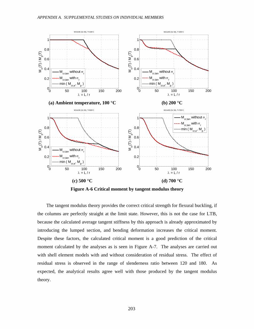
APPENDIX A. SUPPLEMENTAL STUDIES ON INDIVIDUAL MEMBERS
203
0 50 100 150 2000
0.2
0.4
0.6
0.8
1
λ = L / r
Mcr
(T) /
Mp(T
)
W14x90 (Gr.50), T=100°C
Mcr,tan without σr
Mcr,tan with σrmin ( Mcr,e, Mp )
0 50 100 150 2000
0.2
0.4
0.6
0.8
1
λ = L / r
Mcr
(T) /
Mp(T
)
W14x90 (Gr.50), T=200°C
Mcr,tan without σr
Mcr,tan with σrmin ( Mcr,e, Mp )
(a) Ambient temperature, 100 °C (b) 200 °C
0 50 100 150 2000
0.2
0.4
0.6
0.8
1
λ = L / r
Mcr
(T) /
Mp(T
)
W14x90 (Gr.50), T=500°C
Mcr,tan without σr
Mcr,tan with σrmin ( Mcr,e, Mp )
0 50 100 150 2000
0.2
0.4
0.6
0.8
1
λ = L / r
Mcr
(T) /
Mp(T
)
W14x90 (Gr.50), T=700°C
Mcr,tan without σr
Mcr,tan with σrmin ( Mcr,e, Mp )
(c) 500 °C (d) 700 °C
Figure A-6 Critical moment by tangent modulus theory
The tangent modulus theory provides the correct critical strength for flexural buckling, if
the columns are perfectly straight at the limit state. However, this is not the case for LTB,
because the calculated average tangent stiffness by this approach is already approximated by
introducing the lumped section, and bending deformation increases the critical moment.
Despite these factors, the calculated critical moment is a good prediction of the critical
moment calculated by the analyses as is seen in Figure A-7. The analyses are carried out
with shell element models with and without consideration of residual stress. The effect of
residual stress is observed in the range of slenderness ratio between 120 and 180. As
expected, the analytical results agree well with those produced by the tangent modulus
theory.

APPENDIX A. SUPPLEMENTAL STUDIES ON INDIVIDUAL MEMBERS
204
0 50 100 150 2000
0.2
0.4
0.6
0.8
1
1.2
λ = L / ryM
cr(T
) / M
p(T)
W14x90 Fy=345MPa T=500°C
Shell w/o σr
Shell w/ σr
TMT w/o σr
TMT w/ σr
Figure A-7 Comparison of the critical moment by analyses and tangent modulus theory
A.2 MODELING COMPARISON OF INDIVIDUAL MEMBERS
A.2.1 Fiber Model
The influence of local buckling to the critical strength is investigated in this section by
comparing the strength simulated with shell element models and fiber models. The beam
theory (i.e., plane-section-remains-plane assumption) is adopted for the fiber models so that
local buckling is not simulated. The modeling hypotheses for the fiber models are similar to
those for the shell element models. Additional hypotheses specifically applied to the fiber
models are summarized in the following points:
1 Residual stress is not considered.
2 A member is subdivided into 32 elements along its length and each element has three
sections at the ends and center. Displacements between the sections are interpolated
by quadratic functions.
3 The element stiffness matrices are calculated by Gauss’s integration method with two
integration points along with the length and Simpson’s rule is used for calculation of
the section properties. The integration points in a section are shown in Figure A-8.
The difference of the critical strength calculated with the shell element models and fiber
models is not necessarily due to the local buckling, but may be derived from other factors
such as numerical error or modeling assumptions. Therefore, the effect of the local buckling

APPENDIX A. SUPPLEMENTAL STUDIES ON INDIVIDUAL MEMBERS
205
is also studied by introducing an imperfection for local buckling to the shell element models.
If local buckling is the dominating mechanism to the critical strength, it must be sensitive to
the imperfection. The critical imperfection mode for local buckling (denoted as LBb ) is
defined as the lowest local buckling mode obtained by linear buckling analysis. The
imperfection mode is scaled such that the maximum initial displacement is equivalent to
1/1000 of the single local buckling length and the critical imperfection is provided as
translational initial displacements.
Figure A-8 Integration points in fiber model section
A.2.2 Effect of Local Buckling
In this section, the critical axial strengths of columns at an elevated temperature (500 °C) are
investigated under varied member lengths. The column section is a W14×90 (AISC, 2005)
and flexural buckling about strong and weak axes is simulated with four different analytical
models: (1) shell element models with residual stress rσ and without a critical imperfection
for local buckling LBb , (2) shell elements model with rσ and LBb , (3) shell elements model
without rσ and with LBb , and (4) fiber models (no rσ or LBb ). The simulated critical
strengths with the models (2)-(4) are normalized with the strength of model (1) and shown in
Figure A-9.
Residual stress is not considered in models (3) and (4). Consequently, the evaluated
critical strengths are unconservative compared to those with model (1) (more than 1.0 in
Figure A-9). This trend is more clearly observed in the strengths against buckling about the
weak axis and the unconservativeness is 15.9 % at maximum. The strengths of these two
models agree well with each other except when the slenderness ratio equals 20, where local
buckling dominates in model (3). The effect of the local buckling is also observed at the
slenderness ratio of 20 by comparing the critical strengths of models (1) and (2). The

APPENDIX A. SUPPLEMENTAL STUDIES ON INDIVIDUAL MEMBERS
206
strengths of these models are close (the values in Figure A-9 are close to 1.0). Strength
deterioration due to the local buckling at this slenderness ratio is approximately 10 % for
both the strong and weak axes. Corresponding lengths with this slenderness ratio are 3.12m
and 1.89 m for columns subjected to buckling about strong axis and weak axis, respectively.
Considering that buckling about the weak axis is more critical for columns and 1.89 m is
much shorter than a typical column length, limited practical impact of local buckling is
observed in this study.
0 50 100 150 2000.8
0.9
1
1.1
1.2
L / r
Pcr
/ P
cr |
shel
l, σr
W14x90 Fy=345MPa T=500°C Strong Axis
Shell, σr, bLB
Shell, bLBFiber
0 50 100 150 2000.8
0.9
1
1.1
1.2
L / r
Pcr
/ P
cr |
shel
l, σr
W14x90 Fy=345MPa T=500°C Weak Axis
Shell, σr, bLB
Shell, bLBFiber
Strong axis Weak axis
Figure A-9 Effect of imperfection for local buckling
A.2.3 Post Buckling Strength
Depending on the existence of an alternative load carrying path, failure of individual
members in framed structures may not lead to the global structural collapse. Accurate
simulation of this global building collapse is generally difficult due to the complex behavior.
In this research, introductive studies are performed for global building collapse using the
interior column sub-assembly; however further effort is needed for this research area. Failure
of individual structural members or elements can initiate a global collapse and evaluation of
post critical strength of the individual members may be needed. In this section, post-buckling
strengths of columns are investigated with different analysis modeling assumptions for future
development of research on global collapse simulations.
Figure A-10 shows axial strengths of W14×90 columns at elevated temperature (500 °C)
against flexural buckling about the strong and weak axes. The length of the column is 4 m

APPENDIX A. SUPPLEMENTAL STUDIES ON INDIVIDUAL MEMBERS
207
and the corresponding slenderness ratios are 25.6 and 42.3 for buckling about the strong axis
and weak axis, respectively. The simulations are performed with four different models: (1)
fiber model, (2) shell element model without rσ or LBb , (3) shell element model with rσ
and without LBb , and (4) shell element model with rσ and LBb .
0 0.005 0.01 0.0150
0.2
0.4
0.6
0.8
δtop / L
Pcr
(T) /
Py(T
)
W14x90 L=4m 500°C Strong Axis
FiberShellShell, σr
Shell, σr, bLB
0 0.005 0.01 0.0150
0.2
0.4
0.6
0.8
δtop / L
Pcr
(T) /
Py(T
)
W14x90 L=4m 500°C Weak Axis
FiberShellShell, σr
Shell, σr, bLB
(a) Buckling about strong axis (L/ry = 25.6) (b) Buckling about weak axis (L/ry = 42.3)
Figure A-10 Post buckling strength (W14×90, Gr.50, L=4m)
The critical strength with residual stress (model 3) is slightly lower than that without
residual stress (model 2) especially for the weak axis; however, the difference is limited (less
than 5 % difference). The effect of local buckling is influential to post-buckling behavior
(model 3 and 4). This is more clearly observed in the strength against buckling about the
strong axis. Strength calculated with fiber model (model 1), where local buckling is not
simulated, is much higher than the strength with shell element models.
Similar studies are performed for the strength against lateral torsional buckling (LTB)
using the same models. Relationships between uniformly distributed bending moment and
rotation at the end are plotted in Figure A-11(a). The post-buckling moment calculated with
shell element models is significantly lower than the moment of the fiber model due to the
effect of local buckling. Comparing shell element models with and without residual stress
and an imperfection for local buckling, the difference of the bending moment is not
significant. The critical moment of this column is approximately 70 % of the plastic moment
at 500 °C, while it is almost 100 % at ambient temperature with this slenderness ratio.
Vulnerability against LTB is observed at the elevated temperature.

APPENDIX A. SUPPLEMENTAL STUDIES ON INDIVIDUAL MEMBERS
208
0 0.05 0.1 0.15 0.20
0.2
0.4
0.6
0.8
1
θ (rad)
Mcr
(T) /
Mp(T
)Shell, σr, bLB
ShellFiber
0 0.05 0.1 0.15 0.20
0.2
0.4
0.6
0.8
1
θ (rad)
Mcr
(T) /
Mp(T
)
Shell, σr, bLB
Shell, σrShellFiber
(a) Uniformly distributed moment (b) Anti-symmetrically distributed moment
Figure A-11 Post-buckling behavior for LTB
The strength against LTB under anti-symmetric bending moment (linear distribution
along member with minimum and maximum moment at the ends) is also investigated (Figure
A-11(b)). The absolute value of the minimum and maximum moment is equal and the
inflection point is located at the mid-span. LTB will least likely occur under this type of
moment distribution. Therefore, studying these two extreme cases with uniformly and anti-
symmetrically distributed bending moment covers any other cases for risks of LTB under fire
conditions. The assumptions of the study is the same as previous ones (i.e., W14×90 Gr.50 L
= 4 m, 500 °C). An imperfection for LTB is given in the direction of the weak axis, and
takes the form of the sinusoidal curve shown in Eq. (A.16).
2( , , ) sin ,0,0
2000LBL zb x y z
Lπ⎧ ⎫⎛ ⎞= ⎨ ⎬⎜ ⎟
⎝ ⎠⎩ ⎭ (A.16)
The critical bending moments, obtained with the four analysis models, are almost the
same and equal to the plastic moment at the temperature 500 °C. There is no deterioration of
strength due to LTB. The effect of local buckling is again significant to the post buckling
strength. Strength rapidly reduces for the shell element models, while it remains as plastic
moment for the fiber model.

APPENDIX A. SUPPLEMENTAL STUDIES ON INDIVIDUAL MEMBERS
209
A.3 EFFECT OF UNCERTAIN CONDITIONS
A.3.1 Overview
Member-based strength studies are deterministically performed in Chapter 3 to evaluate the
simple design approach described in AISC (2005). Because the approach can give
unconservative member strengths, alternative design equations are proposed. Furthermore,
the AISC method and the proposed equations are probabilistically evaluated in Section 5.3.3
using the defined statistical data (with Table 5-1 in Section 5.2) for the characteristic factors
(loads and steel properties at elevated temperatures). Although this study provides
interesting information regarding the probability of failure considering uncertainties, there
are several aspects, where deterministic conditions are assumed (e.g., uniformly distributed
temperatures, boundary conditions, and imperfections). Evaluation of such conditions is
typically difficult due to the high uncertainty in reality and is not fully performed in this
research. Instead, sensitivities of the critical strength to these conditions are investigated to
understand variation of the actual strength in this section.
Temperature distribution, boundary conditions (rotational constraint stiffness at the
ends), imperfections (residual stress and geometric imperfection), and steel properties at
elevated temperatures are the uncertain conditions whose sensitivities are investigated. The
study is carried out for AISC W14×90 I-shaped steel columns (Grade 50) at 500 °C with
varied member length. The critical strength of the columns is assessed with different values
for each condition and the sensitivities of the strength are evaluated.
A.3.2 Non-uniform Temperature Distribution
Wang (2002) studied the effect of non-uniform temperature distribution within cross-sections
of I-shaped steel columns to the critical strength against buckling about the strong axis. It is
reported that a non-uniform temperature distribution may deteriorate the strength, despite the
average temperature in the sections being lower. Uneven temperature distributions in steel
cross-sections induce bending deformation due to thermal expansion and create P-δ effects.
Consequently, the critical strength may be decreased.
In this research, bucking about the weak axis is studied as a typical failure mechanism of
columns during fires. Figure A-12 and Table A-1 show combinations of non-uniform
temperature distributions in I-shaped steel columns. Temperature is uniformly (500 °C) or

APPENDIX A. SUPPLEMENTAL STUDIES ON INDIVIDUAL MEMBERS
210
linearly (0-500 °C) distributed in a section for the strong direction (S-a and S-b in Figure
A-2) and weak axis direction (W-a, W-b, and W-c). Two symmetric, linearly distributed
temperature distributions for the weak axis are studied (W-b and W-c) in order to study the
combined effect on a the geometric imperfection. The geometric imperfection is represented
by initial distributions that follow a single sinusoidal curve with a maximum displacement of
1/1000 of the column length at the middle. In addition to these non-uniform temperature
distributions within the cross-sections, three types of temperature distributions along the
member length are investigated: uniform (A-a), linear (A-b), and sinusoidal (A-c)
distributions.
Figure A-12 Non-uniform temperature distribution modes
Table A-1 Combinations of non-uniform temperature distributions
Temperature distribution mode Name
along length strong axis in section
weak axis in section
Note
Typical A-a S-a W-a Uniform temperature W-1 A-a S-a W-b Linear for weak axis 1 W-2 A-a S-a W-c Linear for weak axis 2
S A-a S-b W-a Linear for strong axis A-linear A-b S-a W-a Linear in length A-sign A-c S-a W-a Sinusoidal in length
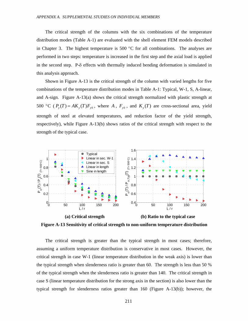
APPENDIX A. SUPPLEMENTAL STUDIES ON INDIVIDUAL MEMBERS
211
The critical strength of the columns with the six combinations of the temperature
distribution modes (Table A-1) are evaluated with the shell element FEM models described
in Chapter 3. The highest temperature is 500 °C for all combinations. The analyses are
performed in two steps: temperature is increased in the first step and the axial load is applied
in the second step. P-δ effects with thermally induced bending deformation is simulated in
this analysis approach.
Shown in Figure A-13 is the critical strength of the column with varied lengths for five
combinations of the temperature distribution modes in Table A-1: Typical, W-1, S, A-linear,
and A-sign. Figure A-13(a) shows the critical strength normalized with plastic strength at
500 °C ( 0( ) ( )y y yP T AK T F= , where A , 0yF , and ( )yK T are cross-sectional area, yield
strength of steel at elevated temperatures, and reduction factor of the yield strength,
respectively), while Figure A-13(b) shows ratios of the critical strength with respect to the
strength of the typical case.
0 50 100 150 2000
0.2
0.4
0.6
0.8
1
L / r
Pcr
(T) /
Py(T
) (T=
500°C
)
TypicalLinear in sec. W-1Linear in sec. SLinear in lengthSine in length
0 50 100 150 2000.4
0.6
0.8
1
1.2
1.4
1.6
L / r
Pcr
(T) /
Pcr
,Typ
(T) (
T= 5
00°C
)
(a) Critical strength (b) Ratio to the typical case
Figure A-13 Sensitivity of critical strength to non-uniform temperature distribution
The critical strength is greater than the typical strength in most cases; therefore,
assuming a uniform temperature distribution is conservative in most cases. However, the
critical strength in case W-1 (linear temperature distribution in the weak axis) is lower than
the typical strength when slenderness ratio is greater than 60. The strength is less than 50 %
of the typical strength when the slenderness ratio is greater than 140. The critical strength in
case S (linear temperature distribution for the strong axis in the section) is also lower than the
typical strength for slenderness ratios greater than 160 (Figure A-13(b)); however, the

APPENDIX A. SUPPLEMENTAL STUDIES ON INDIVIDUAL MEMBERS
212
relative strength does not go lower than 90 % of the typical strength, which is not a
significant deterioration in strength. This non-uniform temperature distribution mode for the
strong axis would have a greater impact, if the critical mechanism under uniform temperature
is buckling about the strong axis. Slender columns are more vulnerable to non-uniform
temperatures within the cross-section. This result is consistent with the study by Wang
(2002). Non-uniform temperature along the member length (A-linear and A-sign in Table
A-1) constantly yields greater critical strengths than the typical strength.
Shown in Figure A-14 are the critical strengths of non-uniform temperature combination
cases W-1 and W-2 in Table A-1. The combined effect of non-uniform temperature
distribution about the weak axis and geometric imperfections are investigated. The
geometric imperfection increases and decreases the bending deformation due to the non-
uniform temperature for W-1 and W-2, respectively. The geometric imperfection does not
impact the strength as much as non-uniform temperature distribution does, because the
critical strength in these two cases is not much different. The effect of the non-uniform
temperature distribution dominates that of the geometric imperfection.
0 50 100 150 2000
0.2
0.4
0.6
0.8
1
L / r
Pcr
(T) /
Py(T
) (T=
500°C
)
TypicalLinear in sec. W-1Linear in sec. W-2
0 50 100 150 2000.4
0.6
0.8
1
1.2
1.4
1.6
L / r
Pcr
(T) /
Pcr
,Typ
(T) (
T= 5
00°C
)
(a) Critical strength (b) Ratio to the typical case
Figure A-14 Sensitivity of critical strength to non-uniform temperature distribution for the weak axis
A.3.3 Imperfections
Sensitivity of the critical strength of the columns at an elevated temperature (500 °C) to
imperfections (geometric imperfection and residual stress) is investigated by changing the

APPENDIX A. SUPPLEMENTAL STUDIES ON INDIVIDUAL MEMBERS
213
magnitude of the imperfection by 200 % and 50 %. The geometric imperfection is modeled
by initial displacements that form a sinusoidal curve along the weak axis. The maximum
initial displacement at the center is 1/1000 of the length for the typical setting. The
displacement is varied to 1/500 and 1/2000 of the length for this sensitivity study. The
residual stress is given by the linear distribution mode shown in Figure 3-5(a) and the
maximum residual stress is 20 % of the yield stress both for tension and compression (for
Grade 50 steel). The proportion of the yield stress and residual stress is assumed as constant
at ambient and elevated temperatures.
Shown in Figure A-15 is the critical strength with different magnitudes of the
imperfections (200 % and 50 % of the original magnitude both for the geometric
imperfection and residual stress). The influence of the geometric imperfection and residual
stress is about the same order and is relatively significant to the members with slenderness
ratio of 100-160. However, since the maximum influence is about 10 % of the critical
strength, the strength can be considered not significantly sensitive to the imperfections.
0 50 100 150 2000
0.2
0.4
0.6
0.8
1
L / r
Pcr
(T) /
Py(T
) (T=
500°C
)
TypicalL / 500L / 20002.0 σr
0.5 σr
0 50 100 150 2000.4
0.6
0.8
1
1.2
1.4
1.6
L / r
Pcr
(T) /
Pcr
,Typ
(T) (
T= 5
00°C
)
(a) Critical strength (b) Ratio to the typical case
Figure A-15 Sensitivity of critical strength to imperfections
A.3.4 Boundary Conditions
The rotational constraint at the boundaries of the members is assumed to be free for the
member-based strength assessment performed in Chapter 3 and Section 5.3.3. This
assumption simplifies the assessment and derives conservative results. The effect of the
boundary conditions (rotational constraint of the column ends) is investigated in this section.

APPENDIX A. SUPPLEMENTAL STUDIES ON INDIVIDUAL MEMBERS
214
The AISC W14×90 I-shaped steel columns (Grade 50) at 500 °C are investigated under
four boundary conditions: (1) free top and bottom (Typical), (2) fixed top and bottom, (3)
fixed, bottom and free, top, and (4) springs top and bottom. The rotational springs are elastic
and given a constraint stiffness that is from the adjacent column (continuing column) and the
beams. The temperature of the continuing column is assumed to remain ambient and the
rotational constraint stiffness from the column is obtained from Eq. (A.17).
0,
31y
rot colcr
E I PkL P
⎛ ⎞= −⎜ ⎟
⎝ ⎠ (A.17)
where ,rot colk is the rotational constraint stiffness from the continuing column. 0E , yI , and L
are the elastic modulus at ambient temperature, moment of inertia about the weak axis, and
the member length, respectively. The member length of the continuing column is assumed to
be the same as the length of the heated column. P and crP are the applied and critical axial
forces of the continuing column, respectively. The ratio of P and crP is approximately
evaluated from the pre-calculated critical axial strength of the column (i.e., P is the critical
strength at 500 °C and crP is the critical strength at ambient temperature with rotationally
free boundary conditions).
The contribution of the beams to the rotational boundary constraint stiffness of the
columns ,rot bmk is calculated by considering the effect of the bolted shear-tab connections.
The initial stiffness of the connection (shown in Figure 4-13) is used for the calculation. The
total constraint stiffness at the column boundary is therefore given as , ,rot col rot bmk k+ .
Shown in Figure A-16 is the strength of the columns under the four boundary conditions
with varied member length. The slender columns are more influenced by the boundary
conditions than stocky columns. The strength with the fixed boundary conditions is about
300 % of the strength with the free conditions at a slenderness ratio of 200. The strength
increase with the bottom end fixed condition is about 50 % of the increase with the both ends
fixed condition, while the increase with the springs is about 75 % (Figure A-16(b)).
The rotational constraint by the connecting beams ,rot bmk is taken into account in this
study in addition to the constraint by the continuing column ,rot colk ; however, ,rot bmk is not

APPENDIX A. SUPPLEMENTAL STUDIES ON INDIVIDUAL MEMBERS
215
included in the interior and exterior sub-assembly models used in chapter 4. The critical
strength with and without ,rot bmk is investigated for the column (W14×90, Grade 50 at 500
°C, length equals 4 m, slenderness ratio equals 42.3). The critical strength with both ,rot colk
and ,rot bmk , with only ,rot colk , and without neither ,rot colk and ,rot bmk are 3660 kN, 3620 kN (99
%), and 2770 kN (76 %), respectively. Therefore, the effect of the beam constraint is only
considered for the critical strength for the sub-assembly study.
0 50 100 150 2000
0.2
0.4
0.6
0.8
1
L / r
Pcr
(T) /
Py(T
) (T=
500°C
)
TypicalFixed endsFixed bottomSpring ends
0 50 100 150 200
1
1.5
2
2.5
3
L / r
Pcr
(T) /
Pcr
,Typ
(T) (
T= 5
00°C
)
(a) Critical strength (b) Ratio to the typical case
Figure A-16 Sensitivity of critical strength to boundary conditions at 500 °C
In a similar manner, the critical strength of the columns at ambient temperature is
investigated with the four boundary conditions as shown in Figure A-17. The constraint
effect is more significant for the slender columns, which is considered with the results from
the 500 °C columns. The strength increase with the spring boundary is about 50 % of the
increase with the fixed ends condition. This increase ratio is lower than the ratio studied for
the columns at 500 °C. This is because the rotational constraint from the continuous columns
,rot colk , based on Eq. (A.17), nearly vanishes. Therefore, the increase of the critical strength
by the rotational constraint from the connecting members is more significant for the columns
at elevated temperatures (because the stiffness of the connecting members is relatively
higher).

APPENDIX A. SUPPLEMENTAL STUDIES ON INDIVIDUAL MEMBERS
216
0 50 100 150 2000
0.2
0.4
0.6
0.8
1
L / r
Pcr
0 / P
y0
TypicalFixed endsFixed bottomSpring ends
0 50 100 150 200
1
1.5
2
2.5
3
3.5
L / r
Pcr
0 / P
cr0,
Typ
(a) Critical strength (b) Ratio to the typical case
Figure A-17 Sensitivity of critical strength to boundary conditions at 20 °C
A.3.5 Steel Properties
The sensitivity of the critical strength of the column to the characteristic properties of steel at
elevated temperatures is investigated in this section. The characteristic properties are the
elastic modulus, the yield strength, and the strength at the proportional limit (proportional
strength), as defined in Eurocode 3 (EC3, 1995). Reduction factors of these properties with
respect to temperatures are defined as the proportion of values at elevated temperatures to
those at ambient temperature as shown in Eq.(A.18).
0
( )( )EE TK TE
= , 0
( )( ) p
pp
F TK T
F= , and
0
( )( ) y
yy
F TK T
F= (A.18)
where 0E , 0pF and 0yF are modulus of elasticity, proportional-limit stress and yield stress
at ambient temperature, respectively, and ( )E T , ( )pF T and ( )yF T are those at elevated
temperature T . Other details about the stress-strain curves defined by EC3 are described in
Section 2.2.2.1.
Statistical properties (mean and coefficient of variation, c.o.v.) of ( )yF T and ( )E T are
defined in Table 5-1 in Section 5.2.1. In addition, the mean and c.o.v. of ( )pF T are assumed
to be 0( )y yK T F and 0.22 (same as c.o.v. of ( )yF T ), respectively, for the study in this

APPENDIX A. SUPPLEMENTAL STUDIES ON INDIVIDUAL MEMBERS
217
section. The critical strength of W14×90 (Grade 50) columns at 500 °C with varied length
are simulated with mean plus and minus one standard deviation of ( )yF T , ( )pF T , and ( )E T
(Figure A-18). The yield strength controls the critical strength of shorter columns
(slenderness ratio of 80 or smaller), while the elastic modulus controls for longer columns
(slenderness ratio of 100 or greater). This is because yielding or plastic buckling is the
critical mechanism for shorter columns and elastic buckling is that for longer columns. The
maximum difference of the critical strength with mean plus and minus one standard deviation
of ( )pF T is approximately 10 % for the columns with intermediate length (around the
slenderness ratio of 80); therefore, the sensitivity of the critical strength to ( )pF T is less than
the sensitivity of the critical strength to ( )yF T and ( )E T .
0 50 100 150 2000
0.2
0.4
0.6
0.8
1
L / r
Pcr
(T) /
Py(T
) (T=
500°C
)
Typical+ Ky(T)- Ky(T)+ Kp(T)- Kp(T)+ KE(T)- KE(T)
0 50 100 150 2000.4
0.6
0.8
1
1.2
1.4
1.6
L / r
Pcr
(T) /
Pcr
,Typ
(T) (
T= 5
00°C
)
(a) Critical strength (b) Ratio to the typical case
Figure A-18 Sensitivity of critical strength to steel properties at 500 °C
The c.o.v.s of ( )yF T , ( )pF T , and ( )E T at elevated temperatures are defined as 0.22,
while those of 0yF and 0E at ambient temperature are 0.1 and 0.06, respectively
(Ellingwood, 1983). The variation of the critical strength due to the uncertainty of the steel
material properties at elevated and ambient temperatures is compared. Shown in Figure A-19
is the sensitivity of the critical strength of the column to 0yF and 0E at ambient temperature.
Due to the difference of the material uncertainties (c.o.v.s), the critical strength varies less at
ambient temperature.

APPENDIX A. SUPPLEMENTAL STUDIES ON INDIVIDUAL MEMBERS
218
0 50 100 150 2000
0.2
0.4
0.6
0.8
1
L / r
Pcr
0 / P
y0Typical+ Ky(T)- Ky(T)+ KE(T)- KE(T)
0 50 100 150 2000.4
0.6
0.8
1
1.2
1.4
1.6
L / r
Pcr
0 / P
cr0,
Typ
(a) Critical strength (b) Ratio to the typical case
Figure A-19 Sensitivity of critical strength to steel properties at 20 °C
A.4 OTHER MISCELLANEOUS STUDIES
A.4.1 Temperature Distribution of Composite Beams
A non-uniform temperature distribution mode for composite beam sections is assumed as
shown in Figure A-20 referring to experimental data obtained by Wainman and Kirby (1988).
The temperature between the lower flange and 3/4 of web is defined as LT , while the
temperatures at the upper 1/4 of web and the upper flange are 0.9 LT and 0.8 LT , respectively.
Figure A-20 Temperature distribution of composite section
Wainman and Kirby (1988) carried out multiple tests for simply supported beams at
elevated temperatures. Temperatures and displacements of the beams were recorded under
constant mechanical load with increasing temperature. One of their typical tests is selected
(data #89) and discussed in this section. Figure A-21 shows the longitudinal section of the
test assembly. The beam is British BS4360, 356×171×67UB Grade 43A ( yF = 292 MPa) and

APPENDIX A. SUPPLEMENTAL STUDIES ON INDIVIDUAL MEMBERS
219
the nominal section properties are shown in Table A-2. The span of the simply supported
beam was 4.5 m. Concrete slab blocks were placed at the top of the steel beam; however,
composite effect was not expected without stud connections between the slab and beam.
Although the tested beam was non-composite, it is a good reference for the temperature
distribution of composite steel beams with concrete slabs.
Table A-2 Section sizes of beam tested by Wainman and Kirby (mm)
Section Web height, h Web thickness, wt Flange width, fb Flange thickness, ft
356×171 364.0 9.1 173.2 15.7
Figure A-21 Beam experiment by Wainman and Kirby (1988)
(Wainman, D. E., Kirby, B. R. (1988), “Compendium of UK Standard Fire Test Data, Unprotected Structural Steel - 2,” Ref. No. RS/RSC/S1199/8/88/B, British Steel Corporation (now Corus), Swinden Laboratories, Rotherham, pp 14 Figure 1(a))
The beam is heated in a furnace and temperatures of the beam at several sections and the
mid-span displacement were recorded. The recorded temperatures at three sections are
shown in Figure A-22. The locations of these three sections were 0.62 m left from the center
(section 1), the center (section 2), and 0.31 m right from the center (section 3) as shown in
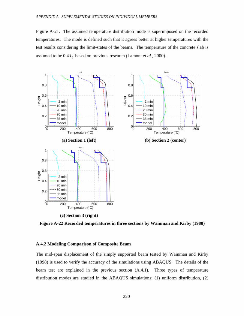
APPENDIX A. SUPPLEMENTAL STUDIES ON INDIVIDUAL MEMBERS
220
Figure A-21. The assumed temperature distribution mode is superimposed on the recorded
temperatures. The mode is defined such that it agrees better at higher temperatures with the
test results considering the limit-states of the beams. The temperature of the concrete slab is
assumed to be 0.4 LT based on previous research (Lamont et al., 2000).
0 200 400 600 8000
0.2
0.4
0.6
0.8
1
Temperature (°C)
Hei
ght
Left
2 min10 min20 min30 min35 minmodel
0 200 400 600 8000
0.2
0.4
0.6
0.8
1
Temperature (°C)
Hei
ght
Center
2 min10 min20 min30 min35 minmodel
(a) Section 1 (left) (b) Section 2 (center)
0 200 400 600 8000
0.2
0.4
0.6
0.8
1
Temperature (°C)
Hei
ght
Right
2 min10 min20 min30 min35 minmodel
(c) Section 3 (right)
Figure A-22 Recorded temperatures in three sections by Wainman and Kirby (1988)
A.4.2 Modeling Comparison of Composite Beam
The mid-span displacement of the simply supported beam tested by Wainman and Kirby
(1998) is used to verify the accuracy of the simulations using ABAQUS. The details of the
beam test are explained in the previous section (A.4.1). Three types of temperature
distribution modes are studied in the ABAQUS simulations: (1) uniform distribution, (2)

APPENDIX A. SUPPLEMENTAL STUDIES ON INDIVIDUAL MEMBERS
221
bilinear distribution (uniform at lower half and linearly interpolated at the upper half with 60
% of the temperature at the top) and (3) detailed distribution calibrated with the recorded
temperatures.
These three temperature modes along the height of the section are compared with the test
data as shown in Figure A-23(a). The temperature distributions from the test were recorded
at the three sections and the lower flange temperatures are around 350-400 °C. The detailed
distribution mode agrees with the test data fairly well, while the uniform mode has a large
temperature gap at the top. Relationships between the mid-span displacement and the
elevated lower flange temperatures are compared in Figure A-23(b) for the test data and
simulations with these three distribution modes. Although the beam had no stud connections
to engages composite behavior, the concrete slab on top of the steel beam significantly
influenced the non-uniform temperature distribution from the test (accordingly, the
simulation were modeled as non-composite). The mid-span displacement from the test is -30
mm at 400 °C of the lower flange temperature. The mid-span displacement calculated by the
simulation with the detailed temperature distribution at this temperature is -24 mm, while
those with bilinear and uniform distribution are -19 mm and -5 mm, respectively. The non-
uniform temperature distribution induced greater mid-span displacement and it is accurately
simulated in the analysis.
0 100 200 300 400 5000
0.2
0.4
0.6
0.8
1
Temperature (°C)
Hei
ght
Test (at 10 min)UniformLinearDetailed
0 200 400 600-200
-150
-100
-50
0
Temperature (°C)
Mid
-spa
n di
sp. (
mm
)
TestUniformLinearDetailed
(a) Temperature distribution (b) Mid-span displacement
Figure A-23 Comparison between analysis and test by Wainman and Kirby (1988)

APPENDIX A. SUPPLEMENTAL STUDIES ON INDIVIDUAL MEMBERS
222
A.4.3 Effect of Heat Conduction
In the structural fire simulations for the frames in the benchmark building, it is assumed that
the temperatures of the members are constant along the member length. Therefore, the
columns above and below the fire compartment remain cool with perfect heat insulation
assumed at the floor level. However, the temperature of these columns near the floors must
elevate due to heat conduction. In order to investigate the temperature of the columns above
and below the fire compartment and evaluate the rationale of the constant temperature
assumption along the member length, the effect of heat convection is studied in this section.
Figure A-24 shows a study model for a one dimensional transient heat conduction
problem. The column in the fire compartment is heated and the temperature is assumed
uniformly constant at 500 °C. The temperature of the column above the fire compartment is
originally 20 °C at time t = 0 along its length. Fire insulation at the floor level is assumed to
be perfect; therefore, the heat transfers from the heated column to the column above only by
conduction (i.e., no radiation or convection). The temperature at the floor level is maintained
at 500 °C and the heat supply to the above column is infinite.
Figure A-24 Study model for heat conduction
The diffusion equation of the column above the fire compartment is stated in Eq. (A.19).
2
2pT Tc kt x
ρ ∂ ∂=
∂ ∂ (A.19)
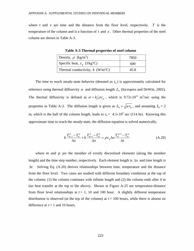
APPENDIX A. SUPPLEMENTAL STUDIES ON INDIVIDUAL MEMBERS
223
where t and x are time and the distance from the floor level, respectively. T is the
temperature of the column and is a function of t and x . Other thermal properties of the steel
column are shown in Table A-3.
Table A-3 Thermal properties of steel column
Density, ρ (kg/m3) 7850 Specific heat, pc (J/kg°C) 600
Thermal conductivity, k (W/m°C) 45.8
The time to reach steady-state behavior (denoted as 0t ) is approximately calculated for
reference using thermal diffusivity α and diffusion length 0L (Incropera and DeWitt, 2002).
The thermal diffusivity is defined as pk cα ρ= , which is 9.72×10⁻⁶ m2/sec using the
properties in Table A-3. The diffusion length is given as 0 0L tα= , and assuming 0L = 2
m, which is the half of the column length, leads to 0t = 4.1×10⁵ sec (114 hr). Knowing this
approximate time to reach the steady-state, the diffusion equation is solved numerically.
1
1 1p p p p p p
m m m m m mp
T T T T T Tk k c xx x t
ρ+
− +− − −+ = Δ
Δ Δ Δ (A.20)
where m and p are the member of evenly discretized elements (along the member
length) and the time step number, respectively. Each element length is xΔ and time length is
tΔ . Solving Eq. (A.20) derives relationships between time, temperature and the distance
from the floor level. Two cases are studied with different boundary conditions at the top of
the column: (1) the column continues with infinite length and (2) the column ends after 4 m
(no heat transfer at the top to the above). Shown in Figure A-25 are temperature-distance
from floor level relationships at t = 1, 10 and 100 hour. A slightly different temperature
distribution is observed (at the top of the column) at t = 100 hours, while there is almost no
difference at t = 1 and 10 hours.

APPENDIX A. SUPPLEMENTAL STUDIES ON INDIVIDUAL MEMBERS
224
0 100 200 300 400 5000
1
2
3
4
Temperature (°C)
Leng
th (m
)
1 hr10 hr100 hr100 hr 4m
Figure A-25 Temperature increase by heat conduction
This study shows a very limited temperature increase on the column above the fire
compartment (e.g., 100 °C up at 1 m from the floor level after 10 hours). The result is
consistent with the previously shown preliminary check using the thermal diffusivity. It does
not mean, however, that the column remains cool and is almost intact after a 10-hour fire in
reality. Partitions of the fire compartment including the insulation at the floor level may
break under such a long-lasting fire and the spreading fire would heat the column. This study
simply investigates the effect of heat conduction and shows that the rationale not to take into
account conduction for relatively short-lasting (less than one hour) compartment fire studied
in this research.
The derived limited effect of heat conduction may be counter-intuitive; however,
simulations using ABAQUS agree with this result. Moreover, Dr. Lamont and Dr. Lane with
Arup have verified it with an independent study using SAFIR, a structural fire analysis
program. Their help and advice based on proficient knowledge regarding structural fire
engineering are greatly appreciated.

225
APPENDIX B REFERENCE EQUATIONS
B REFERENCE EQUATIONS
B.1 CONVERSION OF UNITS
In this thesis, SI units are adopted as the primary unit system. In some cases, converted
values in the US units are also shown for easier understanding for some readers. However,
values are shown only in the US units in some quoted plots (e.g., Figure 2-10 and Figure 2-
12: plots for measured stress-strain curves of steel at elevated temperatures in past studies).
Conversion of the SI and US units is briefly introduced below.
The SI and US units regarding temperatures are Celsius (°C) and Fahrenheit (°F). The
relationships between these units are given in Eq. (B.1)
5 ( 32)9C FT T= − (B.1)
where CT and FT are temperatures in Celsius and Fahrenheit, respectively. Some converted
values are shown in Table B-1
Table B-1 Conversion of temperature units
FT (°F) 70 100 200 300 400 500 600 700 800 900 1000 1100 1200
CT (°C) 21 38 93 149 204 260 316 371 427 482 538 593 649
Table B-2 shows the relationships between the SI and US units for length and force.
Table B-2 Conversion of length and force units
1 inch (in) 1 feet (ft) 1 pound (lb) 1 kilopound (kip) 25.4 mm 0.3048 m 4.448 N 4.448 kN

APPENDIX B. REFERENCE EQUATIONS
226
In addition, relationships of the units for pressure are shown in Table B-3.
Table B-3 Conversion of pressure units
1 kilopound per square inch (ksi) 1 pound per square feet (psf) 6.895 MPa (= 6.895×10⁶ N/m2) 47.88 Pa (= 47.88 N/m2)
B.2 SYMBOLS
Expressions of the symbols used in this research are primarily based on AISC (2005).
However, some of the symbols are differently defined in order to clarify the properties at
elevated temperatures from those at ambient temperature. Some expressions used in the
Eurocode (EC1, 2002 and EC3, 2003) are also introduced. Special care is needed in
introducing the Eurocode symbols because they are fairly different from those in AISC.
Also, the definition of sectional axes is different between AISC and Eurocode (Figure B-1).
Consequently, sectional properties are differently expressed. The symbols used in this
research are compared in Table B-4 with those in AISC and Eurocode for reference.
Figure B-1 Section axes in AISC and Eurocode
Table B-4 Symbols in AISC and Eurocode
Symbol AISC Eurocode Unit Property
wC wC
wI (mm6) Warping constant
0E , ( )E T E E (MPa) Elastic modulus (ambient and elevated temperature)
0yF , ( )yF T yF
yf (MPa) Yield strength (ambient and elevated temperature)
0G , ( )G T G G (MPa) Shear modulus of elasticity (ambient and elevated temperature)
xI xI yI (mm4) Moment of inertia about STRONG axis

APPENDIX B. REFERENCE EQUATIONS
227
Symbol AISC Eurocode Unit Property
yI yI
zI (mm4) Moment of inertia about WEAK axis
J J TI (mm4) Torsional constant
( )EK T ( )Ek T ,Ek θ - Reduction factor for the elastic modulus
( )pK T - ,pk θ - Reduction factor for the proportional limit
( )yK T ( )yk T ,yk θ - Reduction factor for the yield stress
0, cr eP crP crN (N) Elastic critical force for flexural buckling (2D)
0, crx eP - , crit yN (N) Elastic critical force for flexural buckling about strong axis
0, cry eP - , crit zN (N) Elastic critical force for flexural buckling about weak axis
xS xS yW (mm3) Section modulus about STRONG axis
yS yS
zW (mm3) Section modulus about WEAK axis
xZ xZ ,pl yW (mm3) Plastic section modulus about STRONG axis
yZ yZ
,pl zW (mm3) Plastic section modulus about WEAK axis
xr xr yi (mm) Radius of gyration about STRONG axis
yr yr
zi (mm) Radius of gyration about WEAK axis
0λ - λ - Slenderness ratio in Eurocode at AMBIENT temperature for flexural buckling (2D)
0xλ - yλ - Slenderness ratio in Eurocode at AMBIENT temperature for flexural buckling about STRONG axis
0yλ - zλ - Slenderness ratio in Eurocode at AMBIENT
temperature for flexural buckling about WEAK axis
0LTλ - LTλ - Slenderness ratio in Eurocode at AMBIENT
temperature for lateral torsional buckling
( )Tλ - θλ - Slenderness ratio in Eurocode at ELEVATED
temperature for flexural buckling (2D)
( )x Tλ - ,y θλ - Slenderness ratio in Eurocode at ELEVATED temperature for flexural buckling about STRONG axis
( )y Tλ - ,z θλ - Slenderness ratio in Eurocode at ELEVATED temperature for flexural buckling about WEAK axis
( )LT Tλ - , ,LT comθλ - Slenderness ratio in Eurocode at ELEVATED temperature for lateral torsional buckling
0χ - χ - Reduction factor in Eurocode at AMBIENT temperature for flexural buckling (2D)
0xχ - yχ - Reduction factor in Eurocode at AMBIENT temperature for flexural buckling about STRONG axis
0yχ - zχ - Reduction factor in Eurocode at AMBIENT temperature for flexural buckling about WEAK axis

APPENDIX B. REFERENCE EQUATIONS
228
Symbol AISC Eurocode Unit Property
0LTχ - LTχ - Reduction factor in Eurocode at AMBIENT temperature for lateral torsional buckling
( )Tχ - fiχ - Reduction factor in Eurocode at ELEVATED temperature for flexural buckling (2D)
( )x Tχ - ,y fiχ - Reduction factor in Eurocode at ELEVATED temperature for flexural buckling about STRONG axis
( )y Tχ - ,z fiχ - Reduction factor in Eurocode at ELEVATED temperature for flexural buckling about WEAK axis
( )LT Tχ - ,LT fiχ - Reduction factor in Eurocode at ELEVATED temperature for lateral torsional buckling
B.3 DESIGN EQUATIONS OF STEEL AT ELEVATED TEMPERATURES
B.3.1 Eurocode 3
Design equations of steel at elevated temperatures are defined as follows in Eurocode 3
(Eurocode 3, Design of Steel Structures – part 1-2. General rules – Structural fire design,
Draft prEN 1993-1-2, Stage 49 Draft, Brussels, Belgium, 2003, pp 17-20)

APPENDIX B. REFERENCE EQUATIONS
229

APPENDIX B. REFERENCE EQUATIONS
230

APPENDIX B. REFERENCE EQUATIONS
231
B.3.2 AS4100
AS4100 defines bilinear stress-strain relationships for steel at elevated temperatures. The
stress-strain relationships are perfect-plastic, and the reduction factors of elastic modulus
( )EK T and yield strength ( )yK T at elevated temperatures are defined by the following Eqs.
(B.2)-(B.5).
( )EK T = 1.02000 ln
1100
TT
+⎡ ⎤⎛ ⎞
⎜ ⎟⎢ ⎥⎝ ⎠⎣ ⎦
when 0 °C < T ≤ 600 °C (B.2)
= 690 1
100053.5
T
T
⎛ ⎞−⎜ ⎟⎝ ⎠−
when 600 °C < T ≤ 1000 °C (B.3)
( )yK T = 1.0 when 0 °C < T ≤ 215 °C (B.4)
= 905
690T−
when 215 °C < T ≤ 905 °C (B.5)
B.4 TIME-TEMPERATURE RELATIONSHIPS
B.4.1 Parametric Fire Curve
Parametric fire curves (time and gas temperature relationships during fire) defined in
Eurocode 1 (2002) are used in this research for the fire simulations. The equations for the
curves are quoted below for the reference. (Eurocode 1, Actions on structures – part 1-2.
General actions – Actions on structures exposed to fire, Final Draft prEN 1991-1-2, Brussels,
Belgium, 2002, pp 31-33)
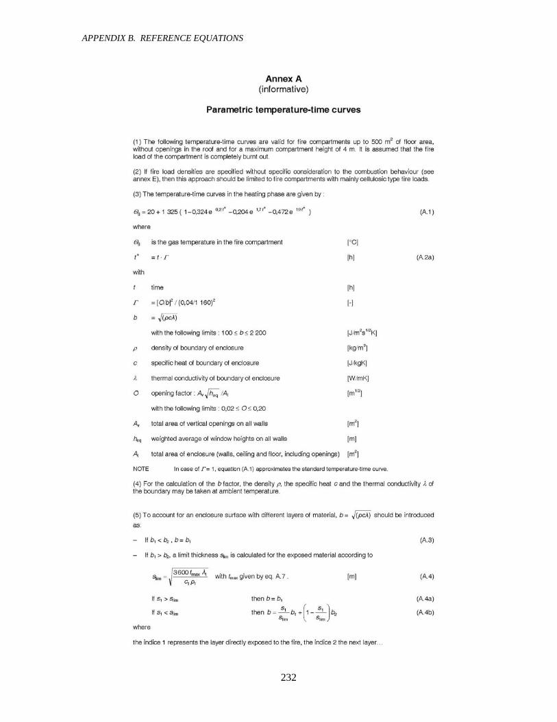
APPENDIX B. REFERENCE EQUATIONS
232
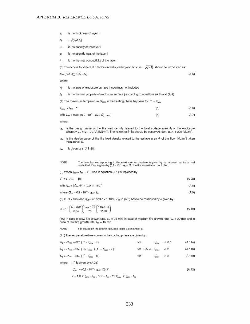
APPENDIX B. REFERENCE EQUATIONS
233

APPENDIX B. REFERENCE EQUATIONS
234
Table B-5 summarizes the parameters and conditions, which are used for the parametric fire
curve equations in this research. These parameters and conditions are set for the simulations
of the compartment fire in the benchmark office building shown in Figure 4-1.
Table B-5 Parameters and conditions for parametric fire curves
Parameter Value or condition
Boundary enclosure material Gypsum
Opening factor, O 0.05
Fire compartment floor area, fA 61 m2
Compartment total surface area, tA 235 m2
Compartment factor, 1qδ 1.5
Occupancy factor, 2qδ 1.0
Fire fighting factor, nδ 0.282
Combustion factor, m 0.8
Some of the parameters in Table B-5 are defined in Eurocode 1 (2002). Part of the
descriptions about the parameters is quoted below for reference. Values used in the fire
simulations in this research are indicated in the original document. (Eurocode 1, Actions on
structures – part 1-2. General actions – Actions on structures exposed to fire, Final Draft prEN
1991-1-2, Brussels, Belgium, 2002, pp 47, 48 and 51)

APPENDIX B. REFERENCE EQUATIONS
235
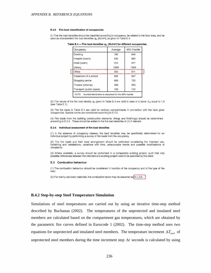
APPENDIX B. REFERENCE EQUATIONS
236
B.4.2 Step-by-step Steel Temperature Simulation
Simulations of steel temperatures are carried out by using an iterative time-step method
described by Buchanan (2002). The temperatures of the unprotected and insulated steel
members are calculated based on the compartment gas temperatures, which are obtained by
the parametric fire curves defined in Eurocode 1 (2002). The time-step method uses two
equations for unprotected and insulated steel members. The temperature increment steelTΔ of
unprotected steel members during the time increment step tΔ seconds is calculated by using

APPENDIX B. REFERENCE EQUATIONS
237
Eq. (B.6). The steel temperature increases by heat transfer from the gas in the fire
compartment. Convection and radiation are the mechanism of the heat transfer for
unprotected steel members under fires. The first and second terms in the outer brackets in
Eq. (B.6) correspond to the convection and radiation, respectively.
4 4,
,
1 { ( ) ( )}steelsteel c steel gas steel steel gas steel
steel steel p steel
FT h T T T T tV c
σερ
Δ = − + − Δ (B.6)
where, steelF and steelF are the surface area and volume of unit length of the steel member,
respectively. ρ is the density, pc is the specific heat, ch is the convection coefficient, ε is
the emissivity, and σ is the Stefan-Boltzmann constant (5.67×10⁻⁸ W/m2°C4). The values of
these constants are shown in Table B-6 (Buchanan, 2002).
On the other hand, the primary mechanism of the heat transfer for the insulated steel
members under fires is conduction. The temperature increment of insulated steel members is
calculated by using Eq. (B.7), where, k is the thermal conductivity, insuld is the thickness of
the fire insulation.
,
,,,
( )(
2
steel p steelsteel insulsteel gas steel
insul insul p insulsteel insul steel p steelsteel p steel
cF kT T T td cFV d c cV
ρρρ ρ
⎡ ⎤⎢ ⎥
Δ = − Δ⎢ ⎥⎢ ⎥+⎢ ⎥⎣ ⎦
(B.7)
Table B-6 Thermal properties of steel and fire insulation
Steel Gypsum Density, ρ (kg/m3) 7850 800 Specific heat, pc (J/kg°C) 600 1700
Thermal conductivity, k (W/m°C) 45.8 0.2 Convection coefficient, ch (W/m2°C) 25 - Emissivity, ε 0.5 -
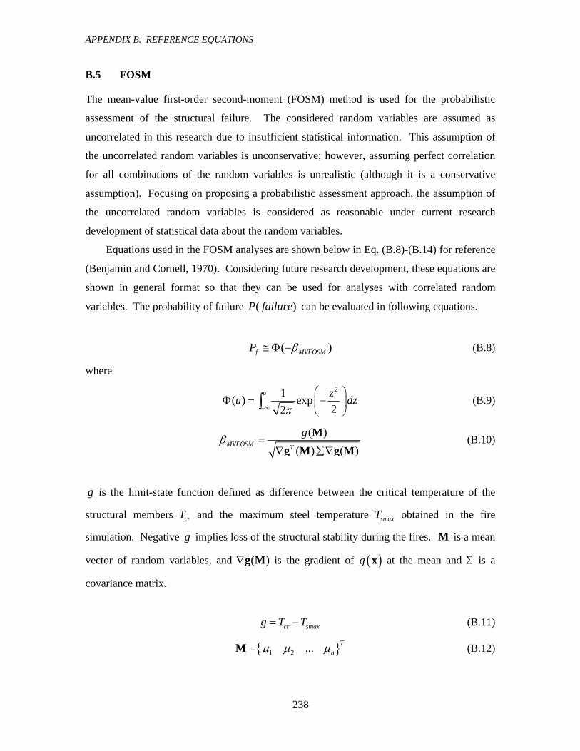
APPENDIX B. REFERENCE EQUATIONS
238
B.5 FOSM
The mean-value first-order second-moment (FOSM) method is used for the probabilistic
assessment of the structural failure. The considered random variables are assumed as
uncorrelated in this research due to insufficient statistical information. This assumption of
the uncorrelated random variables is unconservative; however, assuming perfect correlation
for all combinations of the random variables is unrealistic (although it is a conservative
assumption). Focusing on proposing a probabilistic assessment approach, the assumption of
the uncorrelated random variables is considered as reasonable under current research
development of statistical data about the random variables.
Equations used in the FOSM analyses are shown below in Eq. (B.8)-(B.14) for reference
(Benjamin and Cornell, 1970). Considering future research development, these equations are
shown in general format so that they can be used for analyses with correlated random
variables. The probability of failure ( )P failure can be evaluated in following equations.
( )f MVFOSMP β≅ Φ − (B.8)
where
21( ) exp
22u zu dz
π−∞
⎛ ⎞Φ = −⎜ ⎟
⎝ ⎠∫ (B.9)
( )
( ) ( )MVFOSM T
gβ =∇ ∑∇
Mg M g M
(B.10)
g is the limit-state function defined as difference between the critical temperature of the
structural members crT and the maximum steel temperature smaxT obtained in the fire
simulation. Negative g implies loss of the structural stability during the fires. M is a mean
vector of random variables, and ( )∇g M is the gradient of ( )g x at the mean and Σ is a
covariance matrix.
cr smaxg T T= − (B.11)
{ }1 2 ... Tnμ μ μ=M (B.12)

APPENDIX B. REFERENCE EQUATIONS
239
1 2
( ) ...T
n
g g gx x x
⎧ ⎫∂ ∂ ∂∇ = ⎨ ⎬∂ ∂ ∂⎩ ⎭
g M (B.13)
21 12 1 2 1 1
22 2 2
2
n n
n n
nsym
σ ρ σ σ ρ σ σσ ρ σ σ
σ
⎡ ⎤⎢ ⎥⎢ ⎥Σ =⎢ ⎥⎢ ⎥⎢ ⎥⎣ ⎦
(B.14)
where x is a random variable, μ is a mean, σ is a standard deviation, ρ is a covariance
and n is the number of the random variables.
( )∇g M is approximately calculated in this research in Eq. (B.15).
1 1 1 1
1
( ) ( )( ) ( )( )2 2
T
n n n n
n
g gg g μ σ μ σμ σ μ σσ σ
⎧ ⎫+ − −+ − −∇ = ⎨ ⎬
⎩ ⎭g M (B.15)
The distribution of some random variables (e.g., steel strength at elevated temperatures
and longitudinal constraint stiffness of the beams) is assumed to be lognormal, which is
asymmetric distribution. The lognormal distributions are converted to normal distributions
by taking logarithm and the converted values of mean and standard deviation are used for the
FOSM equations shown above.

APPENDIX B. REFERENCE EQUATIONS
240

241
APPENDIX C JISF EXPERIMENT
C APPENDIX C JISF EXPERIMENT
C.1 SUMMARY
A comparative assessment is performed on experimental data on steel materials at elevated
temperatures provided by the Japan Iron and Steel Federation (JISF). The stress-strain
curves are investigated and compared with the design equations in the Architectural Institute
of Japan (AIJ) and Eurocode 3 (EC3). Statistical information of strength at 1 % and 2 %
strain is evaluated and summarized.
C.2 DATA CONDITIONS
Conditions of the provided test data by JISF are as follows:
(1) Steels with other specifications and grades than those of the steels that JISF provided may
have different characteristics from those of the provided data.
(2) The provided data are all based on basic oxygen furnace steels and electric furnace steels are
not included. When electric furnace steels are included, the data characteristics may be
different due to the differences in production process, chemical compositions, etc.
(3) The steel specimens from which the provided data were obtained are limited in thickness up to
40 mm. The steels with a thickness of over 40 mm may have different characteristics.
(4) The characteristics of steel under elevated temperatures may change when welding or any
type of forming is given to the steel.
C.3 GENERAL
This report summarizes a comparative assessment of experimental data on steel materials at
elevated temperatures provided by the Japan Iron and Steel Federation (JISF) dated on 23
Dec 2003. The data include tensile stress-strain relationships of Japanese standard steel
under ambient and elevated temperatures (20 °C and 300 °C to 800 °C). It is expected that

APPENDIX C. JISF EXPERIMENT
242
the stress-strain relationships obtained in the test will contribute to a better understanding of
behavior of steel structures under fire conditions and fire engineering design, specifically in
establishing reasonably simplified stress-strain curves which can be used for analytical
simulations. The following six different types of steel are examined:
SM490A rolled plate
SM490A wide flange
SM490AW rolled plate
SN490C rolled plate
STKN400B structural tube
STKN490B structural tube
These types of steel are roughly equivalent to Grade 50 mild steel in the US standard
except STKN400B, which has a strength equivalent to Grade 36. Simple data analyses were
performed as part of this assessment to look at two aspects: (1) investigation of the stress-
strain relationships and comparison to those described in Recommendation for Fire Resistant
Design of Steel Structures by Architectural Institute of Japan (AIJ, 1999) and Eurocode 3
(EC3) (CEN, 1995), and (2) statistical study of the strength of the steel at 1 % and 2 % strain
under elevated temperatures.
C.4 JISF STRESS-STRAIN CURVES
Plots of the stress-strain data provided by JISF are shown in Figure C-1 to Figure C-6. Five
sets (five different supplies) of test data are included for each type of steel and each set
contains stress-strain curves under different temperatures (ambient and elevated temperatures
from 300 °C to 800 °C at every 100 °C). Two stress-strain curves are included in each set of
the test data at 400 °C, 500 °C and 600 °C. The test at 800 °C is performed only with
SM490A(PL) and STKN490B steel. As summarized in Table C-1, the total number of tests
is 280. It is observed from the stress-strain curves at elevated temperature shown in Figure
C-1 to Figure C-6 that (1) the yield points and yield plateaus disappear, (2) the stress-strain
relationships become more nonlinear, and (3) strain hardening reduces and disappears.
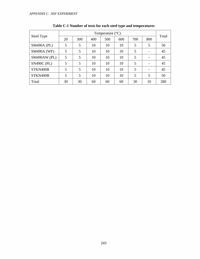
APPENDIX C. JISF EXPERIMENT
243
Table C-1 Number of tests for each steel type and temperatures
Temperature (°C) Steel Type
20 300 400 500 600 700 800 Total
SM490A (PL) 5 5 10 10 10 5 5 50 SM490A (WF) 5 5 10 10 10 5 - 45 SM490AW (PL) 5 5 10 10 10 5 - 45 SN490C (PL) 5 5 10 10 10 5 - 45 STKN400B 5 5 10 10 10 5 - 45 STKN490B 5 5 10 10 10 5 5 50 Total 30 30 60 60 60 30 10 280
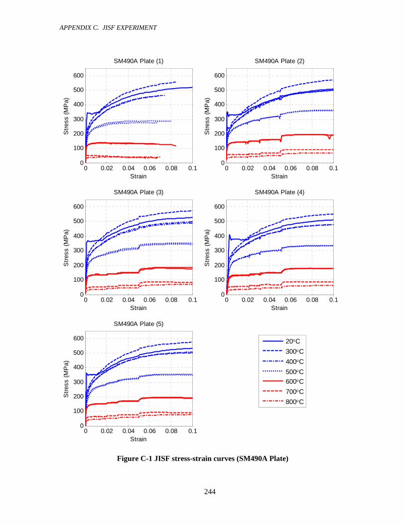
APPENDIX C. JISF EXPERIMENT
244
0 0.02 0.04 0.06 0.08 0.10
100
200
300
400
500
600
SM490A Plate (1)
Strain
Stre
ss (M
Pa)
0 0.02 0.04 0.06 0.08 0.10
100
200
300
400
500
600
SM490A Plate (2)
Strain
Stre
ss (M
Pa)
0 0.02 0.04 0.06 0.08 0.10
100
200
300
400
500
600
SM490A Plate (3)
Strain
Stre
ss (M
Pa)
0 0.02 0.04 0.06 0.08 0.10
100
200
300
400
500
600
SM490A Plate (4)
Strain
Stre
ss (M
Pa)
0 0.02 0.04 0.06 0.08 0.10
100
200
300
400
500
600
SM490A Plate (5)
Strain
Stre
ss (M
Pa)
Figure C-1 JISF stress-strain curves (SM490A Plate)
20°C300°C400°C500°C600°C700°C800°C

APPENDIX C. JISF EXPERIMENT
245
0 0.02 0.04 0.06 0.08 0.10
100
200
300
400
500
600
SM490A Wide Flange (1)
Strain
Stre
ss (M
Pa)
0 0.02 0.04 0.06 0.08 0.10
100
200
300
400
500
600
SM490A Wide Flange (2)
Strain
Stre
ss (M
Pa)
0 0.02 0.04 0.06 0.08 0.10
100
200
300
400
500
600
SM490A Wide Flange (3)
Strain
Stre
ss (M
Pa)
0 0.02 0.04 0.06 0.08 0.10
100
200
300
400
500
600
SM490A Wide Flange (4)
Strain
Stre
ss (M
Pa)
0 0.02 0.04 0.06 0.08 0.10
100
200
300
400
500
600
SM490A Wide Flange (5)
Strain
Stre
ss (M
Pa)
Figure C-2 JISF stress-strain curves (SM490A Wide Flange)
20°C300°C400°C500°C600°C700°C800°C

APPENDIX C. JISF EXPERIMENT
246
0 0.02 0.04 0.06 0.08 0.10
100
200
300
400
500
600
SM490AW Plate (1)
Strain
Stre
ss (M
Pa)
0 0.02 0.04 0.06 0.08 0.10
100
200
300
400
500
600
SM490AW Plate (2)
Strain
Stre
ss (M
Pa)
0 0.02 0.04 0.06 0.08 0.10
100
200
300
400
500
600
SM490AW Plate (3)
Strain
Stre
ss (M
Pa)
0 0.02 0.04 0.06 0.08 0.10
100
200
300
400
500
600
SM490AW Plate (4)
Strain
Stre
ss (M
Pa)
0 0.02 0.04 0.06 0.08 0.10
100
200
300
400
500
600
SM490AW Plate (5)
Strain
Stre
ss (M
Pa)
Figure C-3 JISF stress-strain curves (SM490AW Plate)
20°C300°C400°C500°C600°C700°C800°C

APPENDIX C. JISF EXPERIMENT
247
0 0.02 0.04 0.06 0.08 0.10
100
200
300
400
500
600
SN490C Plate (1)
Strain
Stre
ss (M
Pa)
0 0.02 0.04 0.06 0.08 0.10
100
200
300
400
500
600
SN490C Plate (2)
Strain
Stre
ss (M
Pa)
0 0.02 0.04 0.06 0.08 0.10
100
200
300
400
500
600
SN490C Plate (3)
Strain
Stre
ss (M
Pa)
0 0.02 0.04 0.06 0.08 0.10
100
200
300
400
500
600
SN490C Plate (4)
Strain
Stre
ss (M
Pa)
0 0.02 0.04 0.06 0.08 0.10
100
200
300
400
500
600
SN490C Plate (5)
Strain
Stre
ss (M
Pa)
Figure C-4 JISF stress-strain curves (SN490C Plate)
20°C300°C400°C500°C600°C700°C800°C

APPENDIX C. JISF EXPERIMENT
248
0 0.02 0.04 0.06 0.08 0.10
100
200
300
400
500
600
STKN400B (1)
Strain
Stre
ss (M
Pa)
0 0.02 0.04 0.06 0.08 0.10
100
200
300
400
500
600
STKN400B (2)
Strain
Stre
ss (M
Pa)
0 0.02 0.04 0.06 0.08 0.10
100
200
300
400
500
600
STKN400B (3)
Strain
Stre
ss (M
Pa)
0 0.02 0.04 0.06 0.08 0.10
100
200
300
400
500
600
STKN400B (4)
Strain
Stre
ss (M
Pa)
0 0.02 0.04 0.06 0.08 0.10
100
200
300
400
500
600
STKN400B (5)
Strain
Stre
ss (M
Pa)
Figure C-5 JISF stress-strain curves (STKN400B)
20°C300°C400°C500°C600°C700°C800°C
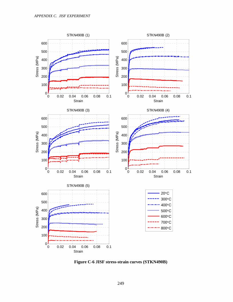
APPENDIX C. JISF EXPERIMENT
249
0 0.02 0.04 0.06 0.08 0.10
100
200
300
400
500
600
STKN490B (1)
Strain
Stre
ss (M
Pa)
0 0.02 0.04 0.06 0.08 0.10
100
200
300
400
500
600
STKN490B (2)
Strain
Stre
ss (M
Pa)
0 0.02 0.04 0.06 0.08 0.10
100
200
300
400
500
600
STKN490B (3)
Strain
Stre
ss (M
Pa)
0 0.02 0.04 0.06 0.08 0.10
100
200
300
400
500
600
STKN490B (4)
Strain
Stre
ss (M
Pa)
0 0.02 0.04 0.06 0.08 0.10
100
200
300
400
500
600
STKN490B (5)
Strain
Stre
ss (M
Pa)
Figure C-6 JISF stress-strain curves (STKN490B)
20°C300°C400°C500°C600°C700°C800°C

APPENDIX C. JISF EXPERIMENT
250
C.5 COMPARISON OF THE TEST DATA WITH AIJ AND EC3
Under current development of structural fire engineering, there are not many design
standards that specify stress-strain curves of steel under elevated temperatures. The
Architectural Institute of Japan (AIJ, 1999) defines stress-strain curves in Recommendation
for Fire Resistant Design of Steel Structures. The AIJ equations are developed to provide
conservative lower strengths that correspond to the mean minus three standard deviations of
strength test data. Additionally, the AIJ curves are configured to provide a more realistic
response for strains larger than 2%.
Eurocode 3 (EC3) (CEN, 1995) is one of the most developed design standards for fire
engineering and defines stress-strain curves that can be used in advanced fire engineering
analysis. The stress-strain curves are established based on data from extensive testing carried
out by Corus (British Steel). Kirby and Preston (1988) summarized the large amount of test
data from Corus and provided useful information of steel properties under elevated
temperatures. The Eurocode curves are the basis of the high temperature provisions of the
American Institute of Steel Construction (AISC) and Australian design standards (AZ4100).
The JISF test data are compared with the AIJ and EC3 equations. Four types of steel
(SM490A, SM490A, SM490AW, and SN490C) are selected for this study as Grade 50 class
rolled steel. The design yield strength of steel and elastic stiffness at ambient temperature are
defined slightly differently by the various design standards, and these properties are the basis
for the design equations for higher temperatures. The AIJ and EC3 equations are calculated
based on steel properties defined in their respective design standards at ambient temperature.
These properties are shown in Table C-2, along with those of AISC.
Table C-2 Elastic modulus and yield strength (Gr.50) defined in AIJ, EC3, and AISC
AIJ EC3 AISC E (GPa) 210 210 200
yF (MPa) 325 355 345
Figures C-7 and C-8 are the plots of the stress-strain relationships of the JISF test data,
and the AIJ and EC3 equations at 300 °C to 700 °C. Figure C-7 shows curves up to 2.5 %
strain and FigurecC-8 shows curves up to 10 % strain. JISF data for 800 °C are limited and
not studied here. The primary range of focus in the EC3 data is on strains less than 2 %,

APPENDIX C. JISF EXPERIMENT
251
because the tangent stiffness vanishes at 2 % strain in EC3 curves. This follows from the fact
that Kirby’s data, upon which EC3 is based, are limited to less than 2 % strain. The AIJ
equations are defined such that they can be used for strains greater than 2 %. Notable
observations from Figure C-7 are: (1) The JISF data have higher variation at higher
temperatures, and (2) The AIJ equation is conservative.

APPENDIX C. JISF EXPERIMENT
252
0 0.005 0.01 0.015 0.02 0.0250
100
200
300
400
500S
tress
(MP
a)
Strain
300 °C
0 0.005 0.01 0.015 0.02 0.0250
100
200
300
400
500
Stre
ss (M
Pa)
Strain
400 °C
300 °C 400 °C
0 0.005 0.01 0.015 0.02 0.0250
100
200
300
400
Stre
ss (M
Pa)
Strain
500 °C
0 0.005 0.01 0.015 0.02 0.0250
50
100
150
200
Stre
ss (M
Pa)
Strain
600 °C
500 °C 600 °C
0 0.005 0.01 0.015 0.02 0.0250
20
40
60
80
100
Stre
ss (M
Pa)
Strain
700 °C
JISFEC3AIJ
700 °C
Figure C-7 Comparison of stress-strain curves (up to 2.5 % strain)

APPENDIX C. JISF EXPERIMENT
253
0 0.02 0.04 0.06 0.08 0.10
100
200
300
400
500
600S
tress
(MP
a)
Strain
300 °C
0 0.02 0.04 0.06 0.08 0.10
100
200
300
400
500
600
Stre
ss (M
Pa)
Strain
400 °C
300 °C 400 °C
0 0.02 0.04 0.06 0.08 0.10
100
200
300
400
Stre
ss (M
Pa)
Strain
500 °C
0 0.02 0.04 0.06 0.08 0.10
50
100
150
200
250
Stre
ss (M
Pa)
Strain
600 °C
500 °C 600 °C
0 0.02 0.04 0.06 0.08 0.10
20
40
60
80
100
120
Stre
ss (M
Pa)
Strain
700 °C
JISFEC3AIJ
700 °C
Figure C-8 Comparison of stress-strain curves (up to 10 % strain)

APPENDIX C. JISF EXPERIMENT
254
C.6 STATISTICAL STUDY
At elevated temperatures, the yield plateau, which is characteristic of structural steel, is no
longer clearly observed and the 0.2 % offset strength is not appropriate to define the yield
strength. Alternatively, the AIJ defines the yield strength as the stress at 1 % strain (1 %
strength), while EC3 defines it as the stress at 2 % strain (2 % strength), where the tangent
stiffness vanishes in the EC3 stress-strain curves. Although either of the definitions can be
used to evaluate the degradation of steel strength, this difference is confusing and makes it
difficult to understand and share experimental data performed in various countries. A large
number of tests for steel under elevated temperatures have been carried out; however, the
results are unexpectedly scattered despite the well-controlled steel quality. The different
definitions of the material properties or different testing procedures may have significantly
influenced these results.
Figures C-9 and C-10 show the stresses of the JISF test data from 300 °C to 700 °C at 1
% and 2 % strain. Four types of steel (SM490A, SM490A, SM490AW, and SN490C) are
selected for this study as Grade 50 class rolled steel. The numbers of the tests are 20 for 300
°C and 700 °C, and 40 for 400 °C to 600 °C. The mean, mean plus and minus one standard
deviation, mean minus three standard deviation, and coefficient of variation (c.o.v.) are
plotted. The mean strength and coefficient of variation are summarized in Table 3. It is
observed that the 1 % and 2 % strength is less closer at higher temperatures (i.e., the 1 %
strength at 300 °C is 84 % of the 2 % strength, while the 1 % strength at 700 °C is 102 % of
the 2 % strength). The c.o.v. has similar relationship with respect to the temperatures (i.e.,
0.06 and 0.05 at 300 °C for 1 % and 2 % strength, respectively; and 0.18 and 0.17 at 700 °C
for 1 % and 2 % strength, respectively).
The AIJ and EC3 equations are superimposed in Figures C-9 and C-10 from 300 °C to
700 °C. The JISF test data agree with EC3 strengths. The 2 % strengths at 100 °C to 400 °C
are generally greater than the strength at ambient temperature; however, EC3 conservatively
defines constant yield strength from ambient temperature up to 400 °C. It is observed,
therefore, that the 2 % strength by EC3 is lower than the test data.
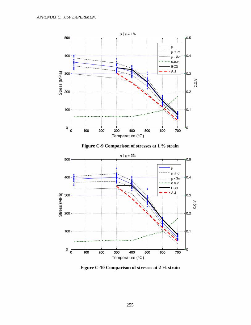
APPENDIX C. JISF EXPERIMENT
255
Figure C-9 Comparison of stresses at 1 % strain
Figure C-10 Comparison of stresses at 2 % strain

APPENDIX C. JISF EXPERIMENT
256
Table C-3 Mean and coefficient of variation of 1 % and 2 % strength
1 % strength 2 % strength Temperature (°C) mean (MPa) c.o.v. mean (MPa) c.o.v.
20 365 0.061 390 0.042 300 337 0.063 399 0.052 400 310 0.062 363 0.049 500 252 0.078 276 0.077 600 146 0.097 148 0.099 700 67 0.176 66 0.172
ACKNOWLEDGEMENTS
Experimental data provided by Japan Iron and Steel Federation are greatly appreciated.

APPENDIX C. JISF EXPERIMENT
257
The following Japanese paper is requested to be attached to this appendix by JISF.
Figure C-11 JISF paper (page 1)

APPENDIX C. JISF EXPERIMENT
258
Figure C-12 JISF paper (page 2)

259
BIBLIOGRAPHY
BIBLIOGRAPHY
Ali, F. A., Shepherd, P., Randall, M., Simms I. W., O’Connor D. J., Burgress I. (1998), “The Effect of Axial Restraint on the Fire Resistance of Steel Columns,” Journal of Constructional Steel Research, 46:1-3 paper No. 177.
Allam, A. M., Burgress, I. W., Plank, R. J. (2002), “Performance-based Simplified Model for
a Steel Beam at Large Deflection in Fire,” Proceeding of 4th international conference on performance-based codes and fire safety design methods, Melbourne, Australia
American Institute of Steel Construction, Inc. (AISC) (1999), “Manual of steel construction
load & resistance factor design,” Chicago, IL. American Institute of Steel Construction, Inc. (AISC) (2005), “Specification for Structural
Steel Buildings,” Chicago, IL. Architectural Institute of Japan (AIJ) (1973), “Design Standard for Steel Structures” Architectural Institute of Japan (AIJ) (1999), “Recommendation for Fire Resistant Design of
Steel Structures,” (in Japanese) Australian Building Code Board (ABCB) (1998), “AS4100-1998, Australian Standard, Steel
Structures” Bailey, C. G. (2005), “Fire Engineering Design of Steel Structures,” Advances in Structural
Engineering, Vol. 8, No. 3, pp185-201 Bailey, C. G., Lennon, T., Moore, D. B. (1999), “The behaviour of full-scale steel-framed
buildings subjected to compartment fires,” The Structural Engineer, 77(8): 15-21.
Bailey, C. G., Burgess, I. W., Plank, R. J. (1996a), “The lateral-torsional buckling of unrestrained steel beams in fire,” Journal of Constructional Steel Research, 1996; 36(2): 101-119.
Bailey, C. G., Burgess, I. W., Plank, R. J. (1996b), “Computer simulation of a full-scale
structural fire test,” The Structural Engineer, 74(6): 93-100.
BIBLIOGRAPHY
260
Baker, D. J., Xie, Y. M., Dayawansa, P. H. (1997), “Numerical Predictions and Experimental Observations of the Structural Response of Steel Columns to High Temperatures,” Fire Safety Science, Proceeding of the Fifth International Symposium, 1997, 1165-1176.
Benjamin, J. R., Cornell, C. A., (1970), “Probability, Statistics, and Decision for Civil
Engineers,” McGraw Hill, Inc. New York. Bredenkamp, P. J., Van den Berg, G. J. (1995), “The strength of Stainless Steel built-up I-
Section Columns,” Journal of Constructional Steel Research Vol 34 No2-3 pp 131-144
Bredenkamp, P. J., Van den Berg, G. J., Van der Merwe, P. (1994 ), “The strength of Hot-
rolled stainless steel columns,” Structural Stability Research Council, Annual Technical Session Proceedings
Burgess, I. W., Olawale, A. O., Plank, R. J. (1992), “Failure of steel columns in fire,” Fire
Safety Journal, 18, 183–201. Buchanan, A. H. (2002), “Structural Design for Fire Safety,” John Wiley & Sons, LTD Custer, R.L.P., Meacham, B.J. (1997), Introduction to Performance-Based Fire Safety,
Society of Fire Protection Engineers, Bethesda, MD., 260 pgs. DeFalco, F. D. (1974), “Investigation of the Compressive Response of Modern Structural
Steels at Fire Load Temperatures,” Ph.D. dissertation, the University of Connecticut Deierlein, G. G., Hamilton, S. (2004) “Framework for Structural Fire Engineering and
Design Methods,” NIST-SFPE Workshop for Development of a National R&D Roadmap for Structural Fire Safety Design and Retrofit of Structures: Proceedings, NISTIR7133, 75-99
Ellingwood, B. (1983), “Probabilistic Codified Design, Theory and Applications,” University
of California Berkeley. European Convention for Constructional Steelwork (ECCS) (2001), “Model Code on Fire
Engineering, First Edition,” ECCS Technical Committee 3, Brussels, Belgium. European Committee for Standardisation (CEN) (2002), “Eurocode 1, Actions on structures –
part 1-2. General actions – Actions on structures exposed to fire,” Final Draft prEN 1991-1-2, Brussels, Belgium.
European Committee for Standardisation (CEN) (1993), “Eurocode 2, Design of Concrete
Structures – part 1-2. General rules – Structural fire design,” ENV 1992-1-2, Brussels, Belgium.
European Committee for Standardisation (CEN) (1995), “Eurocode 3, Design of Steel
Structures – part 1-2. General rules – Structural fire design,” ENV 1993-1-2, Brussels, Belgium.

BIBLIOGRAPHY
261
European Committee for Standardisation (CEN) (2003), “Eurocode 3, Design of Steel Structures – part 1-2. General rules – Structural fire design,” Draft prEN 1993-1-2, Stage 49 Draft, Brussels, Belgium.
Federal Emergency Management Agency (FEMA) 403 (2002), “World Trade Center
Building Performance Study: Data Collection, Preliminary Observations, and Recommendations,” Washington, DC
Franssen, J. M. (2000), “Failure temperature of a system comprising a restrained column submitted to fire,” Fire Safety Journal 34: 191-207.
Franssen, J. M., Schleich, J. B., Cajot, L. G. (1995), “A simple model for the fire resistance
of axially loaded members according to Eurocode 3,” Journal of Constructional Steel Research, 35: 49-69.
Franssen, J. M., Talamona, D., Kruppa, J. Cajot, L. G. (1998), “Stability of steel columns in
case of fire: experimental evaluation,” Journal of Structural Engineering, ASCE 1998; 124(2): 158-163.
Fujimoto, M., Furumura, F., Ave, T., Shinohara, Y. (1980), “Primary Creep of Structural
Steel (SS41) at High Temperatures,” Trans. of Architectural Institute of Japan, 296: 145-157
Fujimoto, M., Furumura, F., Ave, T. (1981), “Primary Creep of Structural Steel (SM50A) at
High Temperatures,” Trans. of Architectural Institute of Japan, 306: 148-156 Galambos, T. V. (1998), “Guide to stability design of criteria for metal structures fifth
edition,” John Wiley & Sons, Inc Hamilton, S.R., Deierlein, G.G., (2004), “Probabilistic Methodology for Performance-Based
Fire Engineering,” Proc. of 5th International Conference on Performance-Based Codes and Fire Safety Design Methods, 6-8 October, 2004, Luxembourg, Society of Fire Protection Engineers, Bethesda, MD., pp327-341.
Harmathy, T. Z., Stanzak, W. W. (1970), “Elevated-temperature Tensile and Creep
Properties of Some Structural and Prestressing Steels,” Fire Test Performance, ASTM STP 464, American Society of Testing and Materials, pp.186-208
Hibbitt, Karlsson & Sorensen (2002), “ABAQUS Version 6.3, User’s Manual,” Hibbitt,
Karlsson & Sorensen, Inc. Incropera, P. F., DeWitt, P. D., (2002), “Introduction to Heat Transfer,” 4th edition, John
Wiley & Sons, Inc. Kirby, B. R., Preston, R. R. (1988), “High Temperature Properties of Hot-rolled Structural
Steels for Use in Fire Engineering Studies,” Fire Safety Journal, 13(1): 27-37.
Kirby, B. R. (1995), “The Behavior of High Strength Grade 8.8 Bolts in Fire,” Journal of Constructional Steel Research, 33, 3-38.

BIBLIOGRAPHY
262
Kirby, B. R. (1997), “Large Scale Fire Tests: The British Steel European Collaborative Research Programme on the BRE 8-Storey Frame,” Proceedings of the 5th International Symposium on Fire Safety Science (IAFSS), Melbourne, Australia, pp.1129–1140.
Kirby, B. R. (1998), “The Behaviour of a Multi-storey Steel Framed Building Subjected to
Fire Attack, Experimental Data,” British Steel (now Corus), Swinden Laboratories, Rotherham.
Lamont, S., Usmani, A. S., Drysdale, D. D., (2000), “Heat Transfer Analysis of the
Composite Slab in the Cardington Frame Fire Tests,” PIT Project Research Report: HT1/HT2, University of Edinburgh
Lawson, R. M. (1990), “Behaviour of Steel Beam-to-column Connections in Fire,” The
Structural Journal, 68(14), 263-271
Lawson, R. M. (2001), “Fire Engineering Design of Steel and Composite Buildings,” Journal of Constructional Steel Research, 57(12), 1233-1247
Liu, J., Astaneh-Asl, A. (2004), “Moment-Rotation Parameters for Composite Shear Tab
Connections,” Journal of Structural Engineering, 130(9), 1371-1380 Liu, T. C. H., Davies, J. M. (2001), “Performance of Steel Beams at Elevated Temperatures
under the Effect of Axial Restraints,” Steel and Composite Structures, Vol.1, No. 4, pp427-440
Lopes, N., Simoes da Silva, L., Vila Real, P. M. M., Piloto P. (2004), “New Proposals for the
Design of Steel Beam-columns in Case of Fire, including a New Approach for the Lateral-torsional Buckling,” Computers and Structures, 2004; 82: 1463–1472.
Ma, K. Y., Richard Liew, J. Y., (2004), “Nonlinear Plastic Hinge Analysis of Three-
Dimensional Steel Frames in Fire,” Journal of Structural Engineering, 130(7), 981-990.
Melchers, R. E. (1999), “Structural Reliability Analysis and Prediction Second Edition,” John
Wiley & Sons Ltd. Moncada, J. A. (2005), “Fire Unchecked,” NFPA Journal March/April 2005 National Bureau of Standards (NBS), U.S. Department of Commerce, (1980), “Development
of a Probability Based Load Criterion for American National Standard A58” National Institute for Land and Infrastructure Management (NILIM), (2005), “Report on the
Windsor Building Fire in Madrid, Spain,” Japan, (in Japanese) National Institute of Standards and Technology (NIST), (2002), “Analysis of Needs and
Existing Capabilities for Full-Scale Fire Resistance Testing,” NIST GCR 02-843, Baltimore

BIBLIOGRAPHY
263
National Institute of Standards and Technology (NIST), (2004), “June 2004 Progress Report on the Federal Building and Fire Safety Investigation of the World Trade Center Disaster, Appendix L- Interim Report on WTC 7,” NIST Special Publication 1000-5.
National Institute of Standards and Technology (NIST), (2005), “Federal Building and Fire
Safety Investigation of the World Trade Center Disaster,” NIST NCSTAR 1. Piloto, P. A. G., Vila Real, P. M. M. (2000), “Lateral Torsional Buckling of Steel I-beams in
Case of Fire - Experimental Evaluation,” Proceedings of the First International Workshop on Structures in Fire, Copenhagen, Denmark, 2000; pp. 95-105.
Poh, K. W., Bennetts, I. D. (1995), “Behavior of Steel Columns at Elevated Temperatures,”
Journal of Structural Engineering, 121(4): 676-684. Ranby, A. (1998), “Structural fire design of thin walled steel sections,” Journal of
Constructional Steel Research, 46(1-3): 303-304 Sanad, A. M., Rotter, J. M., Usmani, A. S., O'Connor, M. A. (2000), “Composite Beams in
Large Buildings under Fire - Numerical Modelling and Structural Behaviour,” Fire Safety Journal, 35(3): 165-188.
SFPE (2007), SFPE Engineering Guide to Performance-Based Fire Protection Analysis and
Design of Buildings, 2nd Ed., Society of Fire Protection Engineers, Bethesda, MD., 224 pgs.
SFPE (2004), Proceedings of 5th International Conference on Performance-Based Codes
and Fire Safety Design Methods, 6-8 October, 2004, Luxembourg, Society of Fire Protection Engineers, Bethesda, MD., 446 pgs.
Simmons, W. F., Cross, H. C. (1955), “Elevated-temperature Properties of Carbon Steels,”
ASTM Special Technical Publication No. 180, American Society for Testing Materials, Philadelphia
Skinner, D. H. (1972), “Measurement of High Temperature Properties of Steel,” BHP
Melbourne Research Laboratories, Report MRL6/10, The Broken Hill Proprietary Company Limited Australia
Suzuki, H., Raungtananurak, N., Fujita, H. (2005), “Research on Behaviors of Steel Frames
Subjected to Fire Heating,” Guidelines for Collapse Control Design II Research, Japanese Society of Steel Construction Council on Tall Building and Urban Habitat: 78-89.
Steel Construction Institute (SCI), (2000), “Fire Safety Design: A New Approach to Multi-
Storey Steel-Framed Buildings,” SCI Publication P288. Steel Construction Institute (SCI), (1991), “Investigation of Broadgate Phase 8 Fire” Takagi, J., Deierlein, G.G., (2007a), “Strength Design Criteria for Steel Members at Elevated
Temperatures,” Journal of Constructional Steel Research, 2007: 63: 1036-1050

BIBLIOGRAPHY
264
Takagi, J., Deierlein, G.G., (2007b), “Stability Investigation of Steel Members and Frames under Fire Conditions,” Annual Stability Conference, Structural Stability Research Council, April 2007, (accepted).
Talamona, D., Franssen, J. M., Schleich, J. B., Kruppa J. (1997), “Stability of Steel Columns
in Case of Fire: Numerical Modelling,” Journal of Structural Engineering, ASCE 1997; 123(6): 713-720.
Talamona, D., Kruppa, J., Franssen, J. M., Recho, N. (1996), “Factors Influencing the
Behaviour of Steel Columns Exposed to Fire,” Journal of Fire Protection Engineers, 8(1): 31-43.
Timoshenko, S. P., Gere, J. M. (1961), “Theory of Elastic Stability Second Edition,”
McGraw-Hill Book Company, Inc Toh, W. S., Tan, K. H., Fung, T. C. (2000), “Compressive Resistance of Steel Columns in
Fire: Rankine Approach,” Journal of Structural Engineering, ASCE 2000; 126(3): 398-405.
United States Fire Administration (USFA), “Interstate Bank Building Fire, Los Angeles,
California (May 4 1988),” Technical Report Series 022 United States Fire Administration (USFA), “High-rise Office Building Fire One Meridian
Plaza, Philadelphia, Pennsylvania (February 23, 1991),” Technical Report Series 046 Uy, B. Bradford, M. A. (1995), “Local Buckling of Cold Formed Steel in Composite
Structural Elements at Elevated Temperatures,” Journal of Constructional Steel Research, 34: 53-73
Vila Real, P. M. M., Cazeli, R., Simoes da Silva, L., Santiago, A., Piloto, P. (2004a), “The
Effect of Residual Stress in the Lateral Torsional Buckling of Steel I-beams at Elevated Temperature,” Journal of Constructional Steel Research, 2004: 60: 783-793.
Vila Real, P. M. M., Franssen, J. M. (2000), “Lateral Torsional Buckling of Steel I-beams in
Case of Fire - Numerical Modeling,” Proceedings of the First International Workshop on Structures in Fire, Copenhagen, Denmark, 2000; pp. 71-93.
Vila Real, P. M. M., Lopes, N., Simoes da Silva, L., Franssen, J. M. (2004b), “Lateral-
torsional Buckling of Unrestrained Steel Beams under Fire Conditions: Improvement of EC3 Proposal,” Computers and Structures, 2004; 82: 1737–1744.
Vila Real, P. M. M., Lopes, N., Simoes da Silva, L., Piloto, P., Franssen, J. M. (2004c),
“Numerical Modeling of Steel Beam-columns in Case of Fire – Comparisons with Eurocode 3,” Fire Safety Journal, 2004; 39: 23-39.
Wainman, D. E., Kirby, B. R. (1988), “Compendium of UK Standard Fire Test Data,
Unprotected Structural Steel - 2,” Ref. No. RS/RSC/S1199/8/88/B, British Steel Corporation (now Corus), Swinden Laboratories, Rotherham.

BIBLIOGRAPHY
265
Wang, Y. C. Moore, D. B. (1994), “The Effect of Frame Continuity on the Critical Temperature of Steel Columns,” Proceedings of the third international KERENSKY conference on global trends in Structural Engineering, Singapore, July
Wang, Y. C. (2002), “Steel and Composite Structures Behaviour and Design fore Fire
Safety,” Spon Press Yu, L. (2006), “Behavior of Bolted Connections during and after a Fire,” Ph.D. Dissertation,
the University of Texas at Austin, Austin, Texas

BIBLIOGRAPHY
266

267
SYMBOLS
SYMBOLS
General Notation
0X and ( )X T indicate that X is a function of temperature.
0X is a property at ambient temperature and ( )X T is that at elevated temperature T .
TX is also used, if the value of X at elevated temperatures is different from that at ambient temperature and X is constant at any elevated temperature.
A = Cross-sectional area (m2)
BA = Cross-sectional area of unthreaded part of bolt (m2)
fA = Cross-sectional area of lumped beam section (half of cross-sectional area of beam) (m2)
wC = Warping constant (m6)
XC = Exponent in equation for proposed critical moment
DL = Dead load
BD = Diameter of bolt (m)
E = Modulus of elasticity (N/m2)
tE = Tangent stiffness (N/m2)
,t aveE = Average tangent stiffness in a section (N/m2)
BvF = Ultimate shearing stress of bolt (N/m2)
LF = Initial yield stress (N/m2)
eF = Elastic buckling stress (N/m2)
pF = Stress at the proportional limit (N/m2)
rF = Residual stress (N/m2)
yF = Yield stress (N/m2)
,y charF = Characteristic 0.2 % off-set yield strength (N/m2)
G = Shear modulus of elasticity (N/m2)
xI , yI = Moment of inertia about strong and weak axis (m4)
J = Torsional constant (m4)

SYMBOLS
268
K = Effective buckling length factor
pK , yK , EK = Reduction factors for the proportional limit, yield stress, and modulus of elasticity respectively
sK = Longitudinal constraint spring stiffness for beams (N/m)
yBK = Reduction factor for bolt shear strength
L = Length (m)
bL = Unbraced length for beams (m)
LL = Live load
pM = Plastic moment (Nm)
rM = Initial yield moment (Nm)
,cr AISCM , ( ,crx AISCM ) = Nominal moment (about strong axis) in AISC (Nm)
, 3cr ECM , ( , 3crx ECM ) = Nominal moment (about strong axis) in EC3 (Nm)
,cr PropM , ( ,crx PropM ) = Proposed nominal moment (about strong axis) (Nm)
,cr eM = Elastic critical moment (Nm)
cr,tanM = Nominal moment by tangent modulus theory (Nm)
uxM = Factored bending moment about strong axis (Nm)
,x endM = Bending moment about strong axis at the ends (Nm)
BN = Number of bolt at connection
BP = Peak strength of longitudinal spring for bolted connections (N)
cP = Vertical load carrying capacity of column (N)
,cr AISCP , ( ,cry AISCP ) = Nominal axial strength of column (for flexural buckling about weak axis) in AISC (N)
, 3cr ECP , ( , 3cry ECP ) = Nominal axial strength of columns (for flexural buckling about weak axis) in EC3 (N)
,cr PropP , ( ,cry PropP ) = Proposed nominal axial strength of column (for flexural buckling about weak axis) (N)
cr,tanP = Nominal strength by tangent modulus theory (N)
gP = Gravity load (N)
nP = Nominal axial strength of column in AISC (N)
sP = Resistance force of vertical spring for interior column (N)

SYMBOLS
269
uP = Factored axial load (N)
uQ = Factored load
BnR = Nominal shear strength of bolt (N)
nR = Nominal resistance in AISC
BtestR = Experimental shear strength of bolt (N)
S = Elastic section modulus (m3)
xS = Elastic section modulus about strong axis (m3)
Z = Plastic section modulus (m3)
xZ = Plastic section modulus about strong axis (m3)
T = Temperature (°C)
LT = Temperature at lower flange of beam (°C)
crT = Critical temperature (°C)
smaxT = Maximum temperature of steel in fire simulation (°C)
dT = Increment of temperature (= T - 20 °C) (°C)
LBb = Critical imperfection mode for local buckling (m)
fb = Flange width of section (m)
pc = Specific heat (J/kg°C)
g = Limit-state function
h = Height of section (m)
ch = Convection coefficient (W/m2°C)
neth = Height of lumped beam section (m)
k = Thermal conductivity (W/m°C) r = Governing radius of gyration (m)
xr , yr = Radius of gyration about strong and weak axis (m)
t = Time (sec)
ft , wt = Flange and web thickness of section respectively (m)
( x , y ) = Coordinate in sections (m)
Δ = Vertical displacement of column (m)
BΔ = Deformation capacity of longitudinal spring for bolted connections (m)
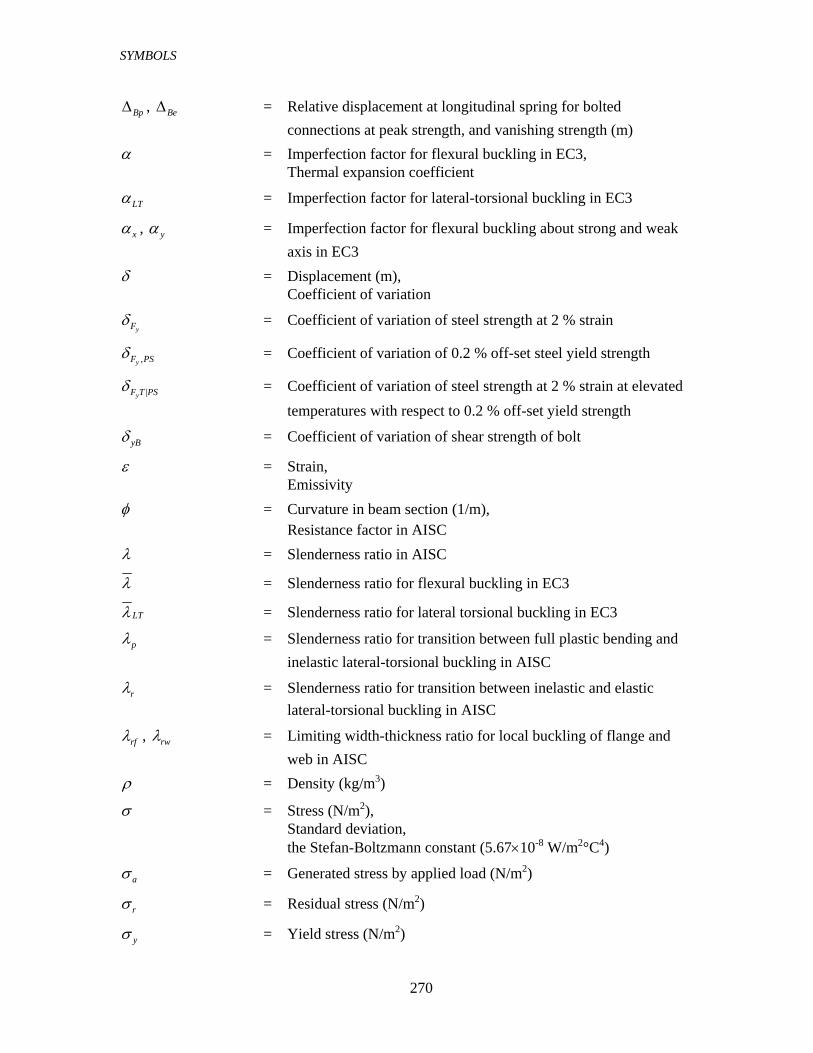
SYMBOLS
270
BpΔ , BeΔ = Relative displacement at longitudinal spring for bolted connections at peak strength, and vanishing strength (m)
α = Imperfection factor for flexural buckling in EC3, Thermal expansion coefficient
LTα = Imperfection factor for lateral-torsional buckling in EC3
xα , yα = Imperfection factor for flexural buckling about strong and weak axis in EC3
δ = Displacement (m), Coefficient of variation
yFδ = Coefficient of variation of steel strength at 2 % strain
,yF PSδ = Coefficient of variation of 0.2 % off-set steel yield strength
|yF T PSδ = Coefficient of variation of steel strength at 2 % strain at elevated temperatures with respect to 0.2 % off-set yield strength
yBδ = Coefficient of variation of shear strength of bolt
ε = Strain, Emissivity φ = Curvature in beam section (1/m), Resistance factor in AISC λ = Slenderness ratio in AISC
λ = Slenderness ratio for flexural buckling in EC3
LTλ = Slenderness ratio for lateral torsional buckling in EC3
pλ = Slenderness ratio for transition between full plastic bending and inelastic lateral-torsional buckling in AISC
rλ = Slenderness ratio for transition between inelastic and elastic lateral-torsional buckling in AISC
rfλ , rwλ = Limiting width-thickness ratio for local buckling of flange and web in AISC
ρ = Density (kg/m3)
σ = Stress (N/m2), Standard deviation, the Stefan-Boltzmann constant (5.67×10⁻⁸ W/m2°C4)
aσ = Generated stress by applied load (N/m2)
rσ = Residual stress (N/m2)
yσ = Yield stress (N/m2)

SYMBOLS
271
μ = Mean
yFμ = Mean of steel strength at 2 % strain (N/m2)
,yF PSμ = Mean of 0.2 % off-set steel yield strength (N/m2)
| ( )yF PS Tμ = Mean of Ratio between 2 % strength at elevated temperatures and
0.2 % off-set strength
Ksμ = Mean of longitudinal spring stiffness for beams by surrounding floor framing (N/m)
yBμ = Mean of shear strength of bolt (N)
yBtestμ = Mean of tested shear strength of bolt (N)
χ = Reduction factor for flexural buckling in EC3
LTχ = Reduction factor for lateral torsional buckling in EC3