Departament d'Economia Aplicada - core.ac.uk · 1. Introduction This paper takes a new look at the hysteresis hypotheses and provides new insights to evaluate the European unemployment

Unemployment, growth and fiscal policy: new insights on the hysteresis

hypothesis

Xavier RaurichHector Sala

Valeri Sorolla

04.04

Facultat de Ciències Econòmiques i Empresarials

Departament d'Economia Aplicada

Aquest document pertany al Departament d'Economia Aplicada.

Data de publicació :

Departament d'Economia AplicadaEdifici BCampus de Bellaterra08193 Bellaterra

Telèfon: (93) 581 1680Fax:(93) 581 2292E-mail: [email protected]://www.ecap.uab.es

Abril 2004

Unemployment, growth and fiscal policy: newinsights on the hysteresis hypothesis∗

Xavier Raurich†

Universitat de Girona and CREB

Hector Sala‡

Universitat Autònoma de Barcelona and IZA

Valeri Sorolla§

Universitat Autònoma de Barcelona

April 23, 2004

Abstract

We develop a growth model with unemployment due to imperfections in thelabor market. In this model, wage inertia and balanced budget rules cause a com-plementarity between capital and employment capable of explaining the existenceof multiple equilibrium paths. Hysteresis is viewed as the result of a selection be-tween these different equilibrium paths. We use this model to argue that, incontrast to the US, those fiscal policies followed by most of the European coun-tries after the shocks of the 1970’s may have played a central role in generatinghysteresis.Key Words: unemployment, hysteresis, multiple equilibria, economic growth,

fiscal policy.JEL Classification Numbers: E24, E62, O41.

∗We thank Jaime Alonso-Carrera for his helpful comments. We are grateful to Spanish Ministry ofEducation for financial support through grants SEC2003-00306 and SEC2003-7928.

†Departament d’Economia, Universitat de Girona, Campus de Montilivi, 17071 Girona, Spain;email: [email protected]; tel.: +34-972.41.82.36.

‡Department d’Economia Aplicada, Universitat Autònoma de Barcelona, Edifici B-Campus UAB,08193 Bellaterra, Spain; tel: +34-93.581.22.93; email: [email protected]

§Departament d’Economia i d’Història Econòmica, Universitat Autònoma de Barcelona, Edifici B,08193 Bellaterra, Spain. tel.: +34-93.581.27.28. e-mail: [email protected].

1. Introduction

This paper takes a new look at the hysteresis hypotheses and provides new insights toevaluate the European unemployment problem. More precisely, the aim of this paperis to provide an explanation of the following two empirical regularities that have notreceived sufficient attention: i) the close correlation between the unemployment ratetrajectory and the growth rate of the capital stock; and ii) the existence of two regimes(this being the central feature of the hysteresis hypotheses) in the unemployment rateand the growth rate of capital stock. In contrast with most of the existing literature, wetake a dynamic general equilibrium approach and explain these empirical regularitiesas the result of equilibria selection in an endogenous growth model with wage inertia,where direct taxes are set by the government to balance its budget constraint.The fact that European labor markets have never recovered the full employment

levels which characterized the 1960s and first 1970s remains as one of the main puzzlesin economics. Among the major conceptions of the labor market analysis, the hysteresishypothesis tackles this puzzle outlining the role played by the extremely persistenteffects of the temporary shocks occurred in the 1970s. Within the studies explainingunemployment hysteresis, we should differentiate between those arguing that temporaryshocks have persistent effects on unemployment because the speed of convergence isextremely low, and those arguing that temporary shocks have persistent effects becausethese shocks make agents coordinate to another equilibrium path, where the economyremains when the shock is over. Our paper belongs to the latter line of research, andexplains the patterns of unemployment as a result of equilibrium selection.Blanchard and Summers (1988) argued that it was necessary to go beyond the nat-

ural rate hypothesis and concluded that “theories of fragile equilibria [a concept tohighlight the sensitive dependence of unemployment on current and past events] arenecessary to come to grip with events in Europe”. Despite this claim, the work on mul-tiple equilibria has not played a major role in the literature. Two main contributions inthis area are Diamond (1982) and Mortensen (1989), but in the context of search andmatching models, which fall well apart from the dynamic general equilibrium approachwe propose in this paper. From the more traditional perspective of the demand-supplyside analysis, Manning (1990 and 1992) argued in favor of models with multiple equi-libria to explain the postwar behavior of unemployment. Nonetheless, the mainstreamliterature on unemployment in the 1990s has kept apart from the multiple equilibriaperspective and, following the work by Layard, Nickell and Jackman (1991), has focusedmainly on the NRU/NAIRU (i.e., a unique unemployment equilibrium rate), leavingalso the hysteresis hypothesis a secondary role. Some work is, of course, being done onthe hysteresis hypotheses, but mainly with an empirical concern.1 Part of this literatureis related with the finding of multiple equilibria in unemployment rates, generally bythe use of Markow regime switching models. For example, in León-Ledesma-McAdam(2003) the presence of a high and low equilibria in most of the Central and EasternEuropean countries is observed; Akram (1998 and 1999) applies this analysis to Nor-way and, finally, Bianchi and Zoega (1998) find that the observed persistence in the

1Some examples are Cross (1988 and 1995), and some papers therein that relate the hysteresishypothesis with the NRU; Jaeger and Parkinson (1994) and, recently, Piscitelli, Cross, Grinfeld andLamba (2000), Hughes Hallet and Piscitelli (2002) and León-Ledesma-McAdam (2003), on the empir-ical testing of the hysteresis hypotheses.

2

unemployment rate of 15 OECD countries is consistent with multiple equilibria models.Given the empirical bias of this work, the main sets of candidates for explaining

hysteresis are still the ones initially proposed in Blanchard and Summers (1986a and1986b), a first one pointing to insider-outsider arguments, a second one to capitalaccumulation (either in the form of physical or human capital) and a third one to fiscalpolicy. In contrast with the extensive literature on the insider-outsider argument (seeamong many others Lindbeck and Snower (2001)), the other two explanations havereceived little relative attention in the theoretical literature. In particular, on the onehand, Coimbra, Lloyd-Braga and Modesto (2000) and Ortigueira (2003) are among thefew exceptions arguing that a low accumulation of capital may explain persistent highunemployment rates.2 On the other hand, Den Haan (2003) and Rocheteau (1999) show,in the framework of a matching model without capital accumulation, that balancedbudget rules may yield multiple steady states. Actually, these authors develop theoriginal argument by Blanchard and Summers (1986b) and show that balanced budgetrules may turn the effects on unemployment of a temporary shock persistent, andeventually, permanent.In contrast to the mainstream theoretical literature, generally overlooking the close

relation displayed by the data between capital accumulation and unemployment,3 weoutline the central role of fiscal policies in the framework of an endogenous growth modelwhere, because of wage inertia, capital stock growth is found to have permanent effectson employment: labor demand is continuously shifted up by capital accumulation,thereby causing a permanent effect on the employment rate because the wage, due toits inertia, does not fully adjust. In this framework, we show that balanced budget rulesmay provide an explanation of the hysteresis hypothesis in the patterns of employmentand economic growth.We consider a simple one-sector endogenous growth model with a linear production

technology where, for simplicity, we let a union set the wage as a mark-up over areservation wage, assumed to be a weighted average of past labor income and, thus,taking account of wage inertia. By means of direct taxes, the government finances publicspending and subsidies, aiming to maintain a balanced budget rule. To this end, eithergovernment spending or direct taxes must be endogenous and adjust to keep the budgetconstraint balanced. When government spending is treated as endogenous, direct taxrates are constant and, hence, exhibit an acyclical behavior. In contrast, when directtax rates are considered endogenous, we expect them to be countercyclical; i.e., to behigh in bad times and low in good times. This is simply a result from the fact thatgovernment expenditures, such as unemployment benefits, rise in bad times and shrinkin good times.

2Like us, Coimbra, et. al. (2000) argue in favor of multiple steady states, but with an OverlappingGenerations Model with strong increasing returns to scale, which are at odds with the empiricalevidence (see Basu and Fernald (1997)). In turn, our approach also differs from Ortigueira (2003),whose analysis is based on a model of labor search with frictional unemployment and human capitalaccumulation.

3Some empirical literature show that there is a close relationship between these two variables. Thisis outlined by Rowthorn (1999) who suggests “that a major factor behind persistent unemploymentmay also be inadequate growth in capital stock”. Henry, Karanassou and Snower (2000) point to theimportance of the role of capital stock in influencing the UK unemployment trajectory, but it is inKaranassou, Sala and Snower (2003) where a reappraisal of the causes of european unemployment isprovided, and capital stock is shown to be an important determinant (if not the leading one) of themovements in the European unemployment rate.

3

When direct tax rates are assumed to be exogenous and constant, the higher iseconomic growth the higher capital accumulation and the more the labor demand shiftsup. Thus, employment is enhanced, provided the rise in labor demand does not fullytranslate into wage increases, which happens when wage inertia is sufficiently strong.In Section 4, we show that the equilibrium path of this simple model with exogenoustaxes is unique and conclude that fails to explain hysteresis.When direct taxes are assumed to be endogenous, these taxes introduce a comple-

mentarity between capital accumulation and employment able to make agents’ expec-tations self-fulfilling and, hence, generate multiple equilibrium paths. To see it, assumethat agents coordinate into an expectations of high net interest rate. If agents arewilling to substitute consumption intertemporally, the savings rate will be large andso will be the growth rates of capital stock and labor demand. When there is wageinertia, the latter implies high values of the employment rate and, thus, strong eco-nomic activity, implying large government revenues and low government expenditures.Obviously, the endogenous direct tax rate will be low and hence the equilibrium interestrate net of taxes will be large, which ensures that agents’ expectations hold in equilib-rium. This explains the existence of an equilibrium path corresponding to an economicregime of high economic activity and, analogously, it can also explain the existence ofanother equilibrium path corresponding to a low regime. In Section 5, we show that theassumption of endogenous taxes may cause the existence of two different equilibriumpaths converging to different steady states. One of them corresponds to a high regimecharacterized by high employment, savings and growth rates, and low direct tax rates,whereas the other one is a regime characterized by low employment, growth and savingsrates, and high tax rates. Along these two equilibrium paths, government spending asa fraction of income is constant, thus, both paths converge to different steady statesthat belong to different sides of the same Laffer curve. In this context, we interprethysteresis as the result of equilibrium selection between these two paths belonging tothe same Laffer curve.The assumptions on the fiscal policy drive the transition. When tax rates are exoge-

nous, employment and the savings rate are negatively related, as a larger employmentrate causes a positive wealth effect that reduces the savings rate. In contrast, when taxrates are endogenous, employment and the savings rate display, along the two equilib-rium paths, a positive correlation due to a substitution effect. In that case, a largeremployment rate implies a lower direct tax rate and, hence, larger net interest andsavings rates.The model allows us to derive a number of necessary conditions to generate hys-

teresis. These are: i) Strong wage rigidities; ii) Endogenous (countercyclical) tax rates;and iii) Large willingness to substitute consumption intertemporally. These conditionspoint to the relevance of the link between labor market institutions and fiscal policy.According to our model, hysteresis may only occur when institutions introduce strongwage inertia and direct tax rates follow a countercyclical pattern.Our model matches remarkably well some observed regularities explained in Section

2. In particular, using Kernel density functions, we show that most of the Europeaneconomies display high and low regimes in unemployment and the growth rate of capitalstock, whereas the US economy displays a unique regime in unemployment. Interest-ingly, direct taxes seem to have been acyclical in the US economy, in contrast with mostof the European ones, where they have tended to be countercyclical. This suggests that

4

the experience of the US corresponds to our scenario of exogenous taxes and a uniqueequilibrium path, whereas the European experience seems to fit with the case wheredirect tax rates are used to balance the government budget constraint and differentequilibria exist. Thus, we are able reinterpret the different consequences of the shockssuffered by these two areas in the 1970s, whose main expression was a temporal down-turn in total factor productivity (TFP). In the US, direct tax rates were kept constantand the TFP downturn produced a temporary fall in savings, economic growth andemployment, which progressively recovered to reach the original equilibrium. Therewere no permanent consequences, as the model explains when tax rates are exogenous.In contrast, the European experience seems to correspond to a case where direct taxrates are endogenous and two equilibrium path exist. In that case, the shocks of the1970’s and the resulting temporal TFP downturn may have caused agents to coordinateinto a low regime equilibrium, hence keeping permanent the effects of these temporaryshocks.The structure of the paper is the following. Section 2 provides an evaluation of

the regime changes in unemployment, which we find closely related with the trajectoryof the capital stock growth rate. A countercyclical behavior of the direct tax ratesis also identified for most of the European countries. Section 3 describes a simplegrowth model. The equilibrium is characterized in the following two sections, but intwo different cases: when direct tax rates are exogenous (Section 4) and when they areendogenous (Section 5). Section 6 summarizes our findings and concludes.

2. Empirical evidence underlying our theoretical modelling

In this section we provide evidence on the differences between the European economiesand the US in the path of unemployment and the capital stock growth rates. Asthe model highlights the role of fiscal policies to explain hysteresis, we also study thebehavior of the direct tax rates.The analysis we undertake next is inspired in Bianchi and Zoega (1998) and relies on

the estimation of Kernel density functions to identify regime changes in the time series ofunemployment and the capital stock growth rates. When a time series displays differentregimes, the density of the frequency distribution of that series will be multimodal,with the number of modes corresponding to the number of regimes. Our identificationcriteria is the following. We will consider that a regime exists when the first derivativeof the Kernel density function is zero and the second derivative is negative. This pointindicates the regime mean value, which can be seen as a local maximum (i.e., a pointwith the highest density). When two or more regimes exist, a ‘valley point’ (the firstderivative is zero and the second one is positive) divides the data points in the sample.Those observations with values above the ‘valley point’ will belong to the upper regime,whereas those with values below will belong to the lower regime.We consider two type of regimes shifts. First, temporary, in response to transitory

or persistent shocks, which means that a set of data points remain in the same regimeat most during four consecutive periods. Second, permanent, in response to irreversibleshifts or permanent shocks, which are all shocks that lasted at least five years. Thisallows to disentangle temporary movements from regime shifts.Our database is the same used in Karanassou, Sala and Snower (2003), containing

annual data on unemployment, business capital stock, GDP and direct taxes, all pro-

5

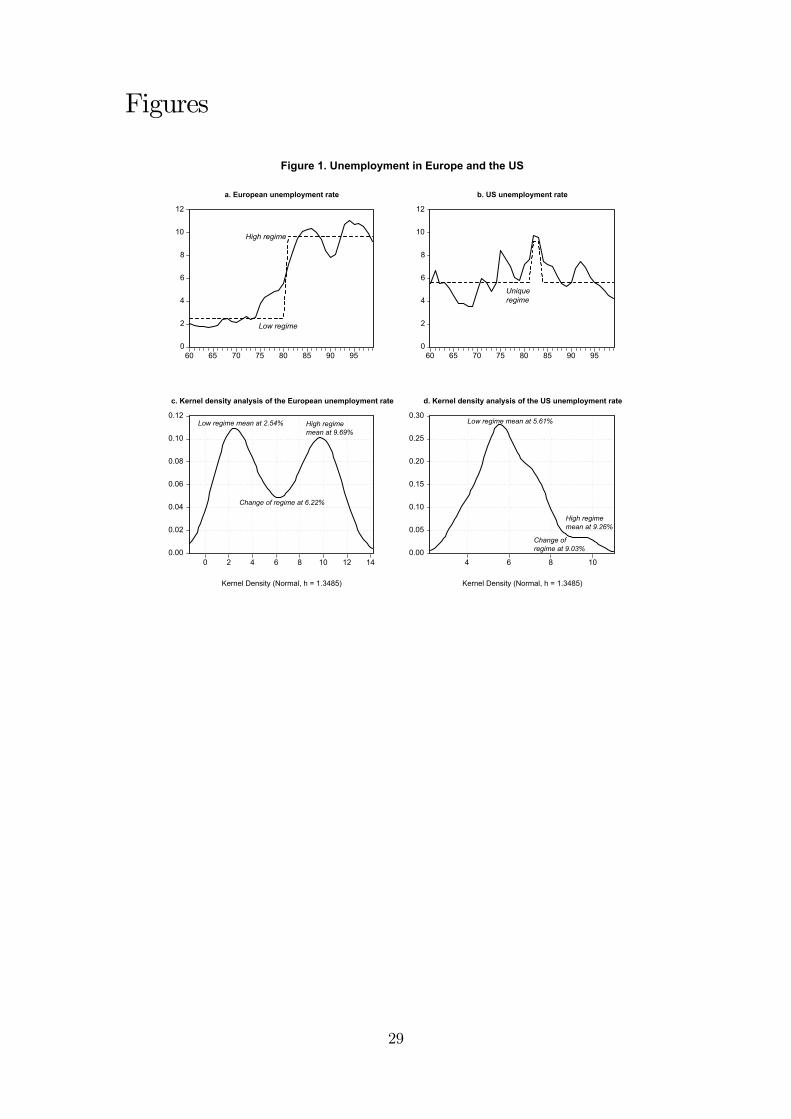
vided by the OECD, for 11 European countries starting in the 1960s (Austria, Belgium,Denmark, Germany, Finland, France, Italy, Netherlands, Spain, Sweden and the UnitedKingdom).Figure 1 pictures the sharp contrast between the unemployment rate trajectory in

Europe and the US.

[Insert Figure 1]

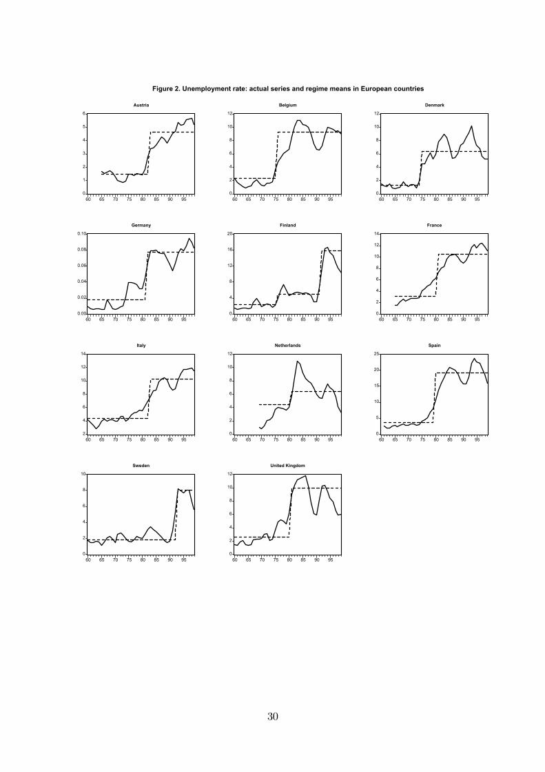
In Europe there is a neat regime shift, placed in 1980 by our Kernel density analysis,which shifts the regime mean upwards from 2.5% to 9.7%. In contrast, the US analysisreveals a unique regime, only altered at the beginning of the 1980s by what seems tohave been a one-off shock. The country-specific analysis, presented in Figure 2, givesadditional evidence on this matter.4

[Insert Figure 2]

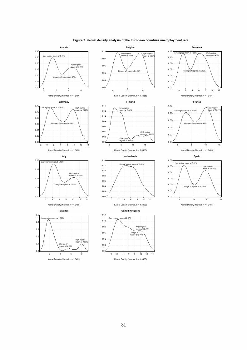
These plots are obtained from the kernel density analysis depicted in Figure 3.

[Insert Figure 3]

It seems clear, thus, that the European has experienced a permanent change, whereasthe US series is characterized by a stationary pattern.Next, we argue that the European countries experienced a permanent change in

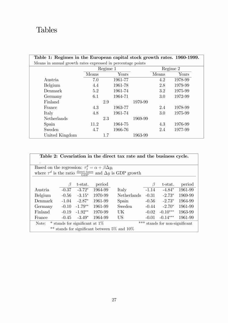
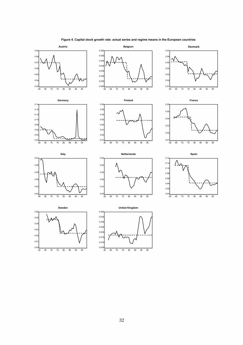
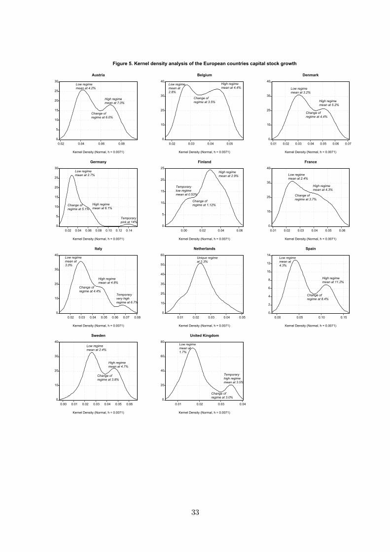
capital formation, with a regime mean shift that corresponds to the regime shift inunemployment. Given the existence of several particular cases, we refer first to thecountry-specific results. In particular, the results of the Kernel density analysis for theindividual countries, pictured in Figures 4 and 5 below, are presented in Table 1.

[Insert Table 1]

Note that in Finland, Netherlands and UK only one regime is identified, whereasthe rest of countries display two regimes.5 All the regime changes take place in the mid1970s, when the unemployment rates in these countries started to rise sharply.

[Insert Figures 4 and 5]

4In Figures 2 and 5 we present only what we consider permanent regime changes (i.e., temporaryregime changes are not plotted, as in Figures 1 and 4) using the criteria explained at the beginning ofthis section.

5In Finland and the Netherlands we only observe a regime because of the lack of data in the 1960s(the series start in 1970 and 1969, respectively), which prevents the Kernel density analysis to considerthe few data points with high values as a separate regime (see figure 5). In Finland, the unique regimediplays a mean of 2.9%, but from 1970 to 1977 capital stock growth is above 3%. In the Netherlandsthe regime mean is at 2.3%, but from 1969 to 1979 takes values above 2.5 percentage points in all yearsexcept 1976.

6

With respect to the aggregate capital stock series for the whole European countries,there is no long time-series directly provided by the OECD. Thus, we need to aggregatethe series corresponding to the pool of countries under consideration, which involvestwo important requirements: first, to establish an accurate criterion to assign countryweights; second, to avoid any noise derived from exchange rates fluctuations, given thatthe capital stock series are expressed in national currencies. The connection betweencapital stock and output point at GDP as the relevant measure to weight the individualcapital stock series. Moreover, GDP series are generally available since the 1960s andthey allow us to compute a yearly weight. To reach the second criterion, we use aseries of real GDP in Purchasing Power Parities. Since we are not interested in theEuropean levels of the capital stock, but on its growth rate, what we finally constructis an aggregate series of the growth rate.6

[Insert Figure 6]

With the aggregate European and US series we conduct a Kernel density analysisand obtain the results displayed in Figure 6. In Figure 6c a first regime is identifiedfor Europe, lasting from 1963 to 1974, and having a mean capital stock growth rateof 4.9%. The second one starts in 1975 and lasts up to 1999, with a regime mean of2.7%. The only exceptional data point in this regime occurs in 1991, when the seriescomes across the German unification consequences, in the form of a sudden rise inthe growth rate of capital stock. The analysis for the US yields a different picture.Despite two regimes are identified (Figure 6d), they differ by just 1.1 percentage points.Following our criterion to qualify the type of regimes, we would identify a high regimemean up to 1985 (with two temporary negative shocks corresponding to the oil pricecrises), followed by a low regime mean which ends by an upwards shift. We interpretthis low regime as a temporal response to a persistent shock that we identify with theanti-inflationist monetary policy of the Volcker era, from 1979 to 1987, which shiftedreal interest rates upwards.Beyond this quantitative analysis, the general picture that emerges is the follow-

ing. In Europe there is a permanent mean shift, which is expressed in an upwardsunemployment regime shift of 7.2 percentage points that, perhaps taking too far ouranalysis, corresponds with a 2.2 percentage points reduction in the mean growth rateof physical capital stock. On the contrary, there is no such a permanent shift in the USunemployment and capital stock. The appropriateness of a multiple equilibria modelfor Europe, assigning a relevant role to capital formation, seems clear.Finally, let’s turn our attention to the path of the direct tax rates. Figure 7 relates

the trajectory of the direct tax rate (as percentage of GDP) to economic growth. Asstated before, we interpret that the negative relationship of these two series correspondsto our scenario of endogenous tax rates, which seems to fit the experience of most ofthe European countries. In particular, the coexistence of what could be taken as a higheconomic growth regime mean in the 1960s and first 1970s with a low direct tax rate

6For Austria, Belgium, Denmark, Germany and Italy we have data on capital stock since 1960 (onthe growth rate since 1961). Nevertheless, the growth rate of the aggregate capital stock series starts in1963 because since 1962 we also have data for France and the UK, and since 1963 for Spain, all countrieswith substantial weight in the EU. The rest of the countries are progressively taken into account, theweights being amended correspondingly: data for Sweden start in 1965, for the Netherlands in 1968and for Finland in 1969.

7

regime mean (and the opposite in the 1980s and 1990s) is apparent in all the Europeancountries with the sole exception of the UK, where these two series display a very mildnegative correlation, just as in the US. Furthermore, in the latter case, there are signsof procyclical tax rates since the second half of the 1980s.

[Insert Figure 7]

In form of scattered diagrams, the plots of Figure 7 would show the negative correla-tion between the direct tax rate and the growth rate. Table 2 presents the estimates ofthis correlation, which is significant at the 1% significance level in all countries exceptGermany (at 8%), Finland (6%) and, of course, the UK and the US, where it is notsignificant.7

[Insert Table 1]

When focussing on the cyclical behavior of the fiscal policy, the literature also re-veals differences between the fiscal policies in the US and in most of the Europeaneconomies. For example, Buti, Franco and Ongena (1997) provide evidence of an initialcountercyclical reaction in Europe after the shocks of the 1970s.8

It seems, thus, that there is a different fiscal policy pattern in Europe and the US,which leads us to think that the fiscal policy, mainly the pattern of the direct tax rates,may be a relevant factor underlying these two areas’ different labor market performance.This is taken into account in the theoretical model presented in Section 3.

3. The Economy

In order to provide an explanation of the empirical regularities just described, in thissection we develop a simple one sector endogenous growth model with labor marketfrictions.

3.1. Labor market

The production function takes the following functional form:

Y (t) = AK (t)α L (t)1−α k (t)1−α , A > 0, α ∈ (0, 1) ,

where Y (t) is the gross domestic product (GDP),K (t) is the aggregate stock of capital,L (t) is the number of employed workers, and k (t) = K(t)

L(t)is the average stock of capital

per employee. The total factor productivity (TFP) is determined by the technologicalparameter A and the path of the average stock of capital.Perfect competition and profit maximization imply that the competitive factors

payment arer (t) = αAK (t)α−1 L (t)1−α k (t)1−α ,

7These results consist on a very simple regression of the sort of the ones presented in Fatás andMihov (2001), which take the following form: zt = α+ β∆yt + νt,where zt is the fiscal variable and ytis GDP. Table 2 presents the estimated β for the European countries and the US.

8For further evidence, see also Fatás and Mihov (2001b) and Calmfors et al. (2003).

8

andw (t) = (1− α)AK (t)α L (t)−α k (t)1−α .

The latter equation implicitly defines the non-equilibrium labor demand

Ld¡w (t) , K (t) , k (t)

¢=

Ã(1− α)AK (t)α k (t)1−α

w (t)

! 1α

.

Along a symmetric equilibrium (i.e. when k (t) = k (t)), the production functionper employee is

y (t) = Ak (t) ,

where y (t) = Y (t)N(t)

, k (t) = K(t)N(t)

, andN (t) is the aggregate labor supply. The competitivefactor payments along a symmetric equilibrium are

r (t) = αA, (3.1)

and

w (t) =(1− α)Ak (t)

l (t), (3.2)

where l (t) = L(t)N(t)

is the employment rate.From (3.2), we obtain the equilibrium labor demand

ld³w (t) ,ek (t)´ = (1− α)Ak (t)

w (t), (3.3)

Note that the capital stock growth rises the labor demand, which enhances the employ-ment rate provided there is wage inertia.Wage inertia arises from the following simple model of firm-level wage setting, where

a firm-level union sets the wage in order to maximize:

Maxw(t)

V = [(1− τ (t))w (t)− ws (t)]γ Ld¡w (t) ,K (t) , k (t)

¢,

where ws (t) is a reference wage, τ (t) is the direct tax rate and γ > 0 provides ameasure of the weight of the wage gap in the unions’ objective function. Since theunions take the labor demand as given, this is a right to manage model. The solutionto this maximization problem characterizes the wage equation

w (t) =w (t)s

(1− τ (t))³1 + γ

ε(t)

´ ,where ε (t) is the inverse of the price elasticity of the labor demand. When the uniondoes not take into account the externality, ε (t) = − 1

αand the wage equation simplifies

9

to9

w (t) =w (t)s

(1− τ (t)) (1− αγ). (3.4)

The reference wage is a controversial variable in the literature. For example, Blan-chard and Wolfers (2000) argue that it depends on the unemployment benefit, pastwages and social security benefits, among other variables. For the sake of simplicity,we assume that it depends on the following weighted average of the workers’ past laborincome:

ws (t) = ws (0) e−θ t + θ

Z t

0

e−θ(t−i)x (i) di, (3.5)

where ws (0) is the initial value of the reference wage, x (t) is the workers’ average laborincome and θ > 0 provides a measure of the rate of wage adjustment. Note that thehigher θ, the lower is the weight of the past average labor income in determining thereference wage, that is, the lower is the wage inertia. Actually, if the parameter θdiverges to infinite, then the reference wage coincides with the current average income,thus excluding wage inertia.It is important to note that there is an initial condition on ws (0) , as this variable is

determined by past average labor income. Moreover, ws (0) determines the initial wagethat is set by the unions, w (0) . Finally, given the initial wage and the initial stockof capital, the initial employment rate is obtained from the equilibrium labor demandl (0) = ld (w (0) , k (0)) . Thus, when there is wage inertia, the employment rate is astate variable whose transition is driven by the degree of wage inertia.Differentiate (3.5) with respect to time to obtain

ws (t) = θ (x (t)− ws (t)) , (3.6)

where the average labor income is assumed to be

x (t) = (1− τ (t)) l (t)w (t) + λ (1− τ (t)) (1− l (t))w (t)− jw (t) , (3.7)

with λ ∈ (0, 1) , j > 0, λ (1− τ (t))w (t) being the unemployment benefits, and jw (t) atax on the wage.10 From now on, we assume that λ (1− τ (t))− j > 0, since otherwisethe labor income of the unemployed workers would be negative.Because the current average labor income is proportional to the wage and, hence,

to per capita GDP, the wage set by the unions rises with economic growth. Whenthere is no wage inertia, the rise in the labor demand due to economic growth fullytranslates into wage increases preventing employment growth. In contrast, when thereis wage inertia, labor demand increases do not fully translate into higher wages andhence economic growth causes employment to rise. Since sustained growth implies thatthe labor demand grows permanently, wage inertia limits the wage adjustment even inthe long run, implying a positive relation between economic growth and the employmentrate even in the long run. To show this positive relation, next we obtain the path of

9Alternativelly, one could assume a national level union that sets the wage taking into account

capital externalities, that is considering the equilibrium labor demand Ld³w (t) ,ek (t)´. In this case,

the wage equation would be w (t) = w(t)s

(1−τ)(1−γ) .10In our model, these taxes amount to any tax allowing the government to finance its expenditures.

For simplicity, they are modelled as proportional to the wage.

10

the employment growth rate. Combine (3.4), (3.6) and (3.7) to get

ws (t)

ws (t)≡ ξ (l (t) , τ (t)) = θ

·l (t) + (1− l (t))λ

1− αγ− j

(1− τ (t)) (1− αγ)− 1¸.

Log-differentiate (3.4) with respect to time

ws (t)

ws (t)=

w (t)

w (t)− τ (t)

1− τ (t)= ξ (l (t) , τ (t)) , (3.8)

where ξ (l (t) , τ (t)) is the growth rate of the after tax wage. Differentiate (3.3) withrespect to time,

l (t)

l (t)=

k (t)

k (t)− w (t)

w (t),

and combine it with (3.8) to obtain the employment growth rate

l (t)

l (t)=

k (t)

k (t)− τ (t)

1− τ (t)− ξ (l (t) , τ (t)) . (3.9)

The time-path of the employment rate depends on the difference between two growthrates: the capital stock one and the one of wages before taxes. As (3.3) shows, capitalstock growth drives the growth of the labor demand, whereas wage growth providesa measure of the corresponding rise in the labor cost. Thus, (3.9) implies that theemployment rate grows when the rise in the labor demand is larger than the rise in theunit cost of labor.

3.2. Consumers

Assume that there is a unique infinitely lived dynasty in the economy. Let N (t) be thenumber of members of this dynasty that inelastically supply one unit of labor so thatthe aggregate labor supply is equal to N (t). This dynasty maximizes the discountedsum of the utility of each memberZ ∞

0

e−(ρ−n) tÃc (t)1−σ − 11− σ

!dt, ρ− n > 0, σ > 0,

subject to the budget constraint11

c (t) + k (t) = ((1− τ (t)) r (t)− n− δ) k (t) + x (t) ,

where ρ > 0 is the subjective discount rate, σ > 0 is the inverse of the intertemporalelasticity of substitution, n > 0 is the constant population growth rate, and δ > 0 isthe constant depreciation rate.The solution to the dynasty maximization problem is characterized by the growth

rate of consumption per capita

11Note that consumers’ revenues accrue from capital income and from average labor income. Weintroduce the average labor income because we assume a large dynasty.

11

c (t)

c (t)=(1− τ (t)) r (t)− δ − ρ

σ, (3.10)

and the transversality condition

limt→∞

e−(ρ−n)tk (t) c (t)−σ = 0. (3.11)

Denote the growth of the per capita consumption by µ (t) = c(t)c(t)

. By using (3.1) and(3.10), it follows that, along a symmetric equilibrium,

µ (τ (t)) =(1− τ (t))αA− δ − ρ

σ. (3.12)

Having shown that consumption and employment growth depend on fiscal policy,we conclude the description of the economy by characterizing fiscal policy.

3.3. Government

Assume that the government follows a balanced budget rule, so that its budget con-straint is given by the following equation:

τ (t)Y (t) + jN (t)w (t) = G (t) + (N (t)− L (t))λ (1− τ (t))w (t) .

Government revenues accruing from taxes are used to finance non-productive govern-ment spending, G (t) , and the unemployment benefit. Denote by g (t) = G(t)

Y (t)the

fraction of GDP devoted to government spending and rewrite the government budgetconstraint as follows

τ (t)− g (t) = (1− α)

µ(1− l (t))λ (1− τ (t))− j

l (t)

¶.

We consider two different fiscal policies. First, assume that g (t) = g is constantand exogenous, and the government sets the value of the direct tax rate to balanceits budget constraint in each period. In that case, the path of the direct tax rate isendogenous and it is determined by the government budget constraint as the followingfunction of the employment rate:

τ (l (t)) =gl (t) + ((1− l (t))λ− j) (1− α)

l (t) + (1− l (t))λ (1− α). (3.13)

Note that

τ 0 (l (t)) = (1− α)

µ(g − 1)λ+ [1− λ (1− α)] j

[l (t) + (1− l (t))λ (1− α)]2

¶< 0,

as λ (1− τ) > j implies that (g − 1)λ + [1− λ (1− α)] j < 0. Note that τ 0 (l (t)) < 0implies that the endogenous tax rate follows a countercyclical path.As a second fiscal policy, assume that τ (t) = τ is constant and exogenous. In

this case, the government sets the path of government spending to balance its budgetconstraint. This path is the following function of the employment rate:

12

g (l (t)) = τ − ((1− l (t))λ (1− τ)− j)

µ1− α

l (t)

¶. (3.14)

Note that

g0 (l) =(1− α) (λ (1− τ)− j)

l2> 0,

as we assume that λ (1− τ) > j.

3.4. Employment and savings rate

To characterize the equilibrium path, use the resource constraint to derive the pathof savings that summarizes the consumers’ behavior. To this end, use the resourceconstraint.

C (t) +G (t) + S (t) = Y (t) ,

where S (t) are the savings of the economy that correspond to gross investment. Lets (t) = S(t)

Y (t)be the savings rate and rewrite the resource constraint as

s (t) = 1− g (t)− C (t)

Y (t)= 1− g (t)− c (t)

Ak (t),

to obtainc (t)

k (t)= (1− s (t)− g (t))A. (3.15)

Differentiating this equation with respect to time,

s (t) = (1− s (t)− g (t))

Ãk (t)

k (t)− µ (t)

!− g (t) . (3.16)

The growth rate of capital is obtained from the resource constraint

C (t) + K (t) + δK (t) = (1− g (t))Y (t) ,

which can be rewritten in per capita terms as follows

c (t) + k (t) + (n+ δ) k (t) = (1− g (t))Ak (t) .

The growth of the per capita stock of capital is then

k (t)

k (t)= (1− g (t))A− c

k (t)− (n+ δ) ,

which, by using (3.15), becomes

k (t)

k (t)= As (t)− n− δ. (3.17)

Combine (3.16) with (3.17), to obtain a differential equation that drives the equi-librium path of the savings rate

13

s (t) = es (s (t) , τ (t) , g (t) , g (t)) (3.18)

= (1− s (t)− g (t)) [As (t)− n− δ − µ (τ (t))]− g (t) ,

Finally, use (3.9) and (3.17) to obtain the differential equation that drives the equi-librium path of the employment rate

l (t) = el (s (t) , l (t) , τ (t) , τ (t)) (3.19)

= l (t)

µs (t)A− n− δ − ξ (l (t) , τ (t))− τ (t)

1− τ (t)

¶.

Note that the equations characterizing the equilibrium depend on the nature of thefiscal policy (i.e., the tax rate being endogenous or exogenous). This distinction isimportant because we associate economies exhibiting acyclical tax rates (like the USone) with the scenario of exogenous taxes, and economies exhibiting countercyclicaltaxes (like most of the European ones) with the scenario of endogenous taxes. Nexttwo sections describe the equilibrium path of an economy with exogenous tax rates(Section 4) and with endogenous tax rates (Section 5).

4. The equilibrium when tax rates are exogenous

Assume that the tax rate is constant, so that τ (t) = τ and hence τ (t) = 0. As aconsequence, (3.19) simplifies to

l (t) = el (s (t) , l (t)) = l (t) (s (t)A− n− δ − ξ (l (t) , τ)) , (4.1)

and, by using (3.14), (3.18) can be rewritten as

s (t) = es (s (t) , l (t)) = (1− s (t)− g (l (t)))

"s (t)A− n− δ − µ− g0 (l (t)) l (t)

1− s (t)− g (l (t))

#.

(4.2)

Definition 4.1. Given {l0,k0; τ} , an equilibrium with exogenous tax rates is defined by{l (t) , s (t) , g (t)}∞t=0 such that solves (3.14), (4.1), and (4.2), satisfies the transversalitycondition (3.11) and the following constraints: l (t) ∈ [0, 1], s (t) ∈ [0, 1] and g (t) ∈[0, 1] , for all t ≥ 0.To characterize the path of the dynamic equilibrium, first obtain the Balanced

Growth Path (BGP), which is defined as a path along which l (t) and s (t) remainconstant, and consumption, capital and GDP grow at the constant growth rate µ. Byusing l (t) = 0 and s (t) = 0, it is straightforward to show that the employment ratealong a BGP must satisfy the following equation:

Q (l) = ξ (l)− µ = 0.

Thus, along a BGP, the long run economic growth rate coincides with the growthrate of wages. In this simple model, this growth rate is equal to the long run growth

14

rates of capital and, as follows from (3.3), of the labor demand. Thus, the employmentrate attains a BGP when the growth rates of the labor demand and of the wage coincide.It can be shown that Q (l) = 0 has a unique root, which is the unique BGP of the

economy if it belongs to the close interval [0, 1] , and if the corresponding savings rateand fraction of GDP devoted to government spending also belong to this interval. TheBGP value of the employment rate is

l∗ =µ1− αγ

1− λ

¶µµ∗

θ+ 1

¶−µ

λ (1− τ)− j

(1− τ) (1− λ)

¶, (4.3)

where the long run growth rate, obtained from (3.12), is

µ∗ =(1− τ)αA− δ − ρ

σ,

and the long run savings rate, obtained from s (t) = 0, is

s∗ =µ∗ + n+ δ

A.

Note that when there is wage inertia (i.e., when θ does not diverge to infinite), economicgrowth increases the long run employment rate. This relation drives some of the resultsin the following proposition:

Proposition 4.1. Assume that l∗ ∈ [0, 1] and s∗ ∈ [0, 1] . Then,

a) ∂l∗∂A

> 0, ∂l∗∂σ

< 0, ∂l∗∂θ

< 0, ∂l∗∂λ

< 0, ∂l∗∂γ

< 0, ∂l∗∂τ?.

b) ∂µ∗∂A

> 0, ∂µ∗∂σ

< 0, ∂µ∗∂θ= 0, ∂µ∗

∂λ= 0, ∂µ∗

∂γ= 0, ∂µ∗

∂τ< 0.

c) ∂s∗∂A?, ∂s∗

∂σ< 0, ∂s∗

∂θ= 0, ∂s∗

∂λ= 0, ∂s∗

∂γ= 0, ∂s∗

∂τ< 0.

P roof. The proof follows from the BGP value of the variables.

As in any AK growth model, the long run growth rate increases with TFP, A,and with the intertemporal elasticity of substitution, 1

σ. When there is wage inertia,

the employment rate depends positively on the economic growth rate, which explainsthe effects of these parameters on the employment rate. Moreover, if there is positivegrowth, the employment rate increases with the wage rigidity, which is negatively relatedwith the parameter θ. As standard, the employment rate decreases with the replacementratio, λ, and with the weight assigned by unions to the wage gap, γ. The direct taxrate drives two opposite forces. On the one hand, it increases the wage paid by firms,which causes a negative effect on employment. On the other hand, it decreases thelabor income, which reduces wages and enhances employment. The net effect is thusambiguous. Finally, most of the effects of the parameters on the savings rate followfrom the effects on the growth rate. The ambiguous effect of TFP on the savings ratedepends on the magnitude of a wealth and a substitution effect.The acyclical behavior of the direct tax rate in the US can be associated with our

scenario of exogenous tax rates. This version of the model and the relevant values (seeTable 3) are thus used to characterize the US economy in the long-run, which is takenas the benchmark economy with exogenous taxes. Table 3 quantifies the effect of someparameter increases.

15

[Insert Table 3]

Proposition 4.2. The BGP is saddle path stable and, hence, the path of the dynamicequilibrium is locally unique.

P roof. See Appendix.

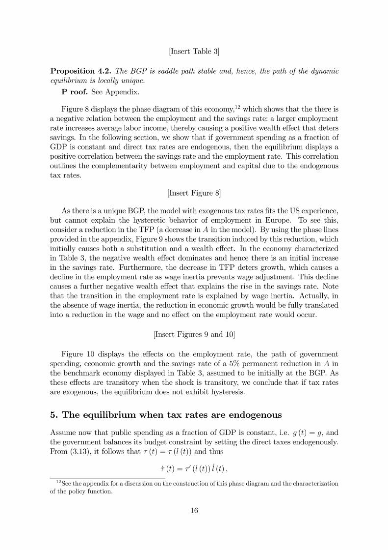
Figure 8 displays the phase diagram of this economy,12 which shows that the there isa negative relation between the employment and the savings rate: a larger employmentrate increases average labor income, thereby causing a positive wealth effect that deterssavings. In the following section, we show that if government spending as a fraction ofGDP is constant and direct tax rates are endogenous, then the equilibrium displays apositive correlation between the savings rate and the employment rate. This correlationoutlines the complementarity between employment and capital due to the endogenoustax rates.

[Insert Figure 8]

As there is a unique BGP, the model with exogenous tax rates fits the US experience,but cannot explain the hysteretic behavior of employment in Europe. To see this,consider a reduction in the TFP (a decrease in A in the model). By using the phase linesprovided in the appendix, Figure 9 shows the transition induced by this reduction, whichinitially causes both a substitution and a wealth effect. In the economy characterizedin Table 3, the negative wealth effect dominates and hence there is an initial increasein the savings rate. Furthermore, the decrease in TFP deters growth, which causes adecline in the employment rate as wage inertia prevents wage adjustment. This declinecauses a further negative wealth effect that explains the rise in the savings rate. Notethat the transition in the employment rate is explained by wage inertia. Actually, inthe absence of wage inertia, the reduction in economic growth would be fully translatedinto a reduction in the wage and no effect on the employment rate would occur.

[Insert Figures 9 and 10]

Figure 10 displays the effects on the employment rate, the path of governmentspending, economic growth and the savings rate of a 5% permanent reduction in A inthe benchmark economy displayed in Table 3, assumed to be initially at the BGP. Asthese effects are transitory when the shock is transitory, we conclude that if tax ratesare exogenous, the equilibrium does not exhibit hysteresis.

5. The equilibrium when tax rates are endogenous

Assume now that public spending as a fraction of GDP is constant, i.e. g (t) = g, andthe government balances its budget constraint by setting the direct taxes endogenously.From (3.13), it follows that τ (t) = τ (l (t)) and thus

τ (t) = τ 0 (l (t)) l (t) ,

12See the appendix for a discussion on the construction of this phase diagram and the characterizationof the policy function.

16

which can be used to rewrite (3.19) as

l (t) = el (s (t) , l (t)) = l (t)

Ãs (t)A− n− δ − ξ (l (t) , τ (l (t)))

1 + τ 0(l(t))l(t)1−τ(l(t))

!, (5.1)

and (3.18) as

s (t) = es (s (t) , l (t)) = (1− s (t)− g) [s (t)A− n− δ − µ (τ (l (t)))] . (5.2)

Definition 5.1. Given {l0,k0; g} , an equilibrium with endogenous tax rates is char-acterized by {l (t) , s (t) , τ (t)}∞t=0 such that solves equations (3.13), (5.1), and (5.2),and satisfies (3.11) and the following constraints: l (t) ∈ [0, 1] , s (t) ∈ [0, 1] , andτ (t) ∈ [0, 1] for all t ≥ 0.The BGP of this economy is obtained when l (t) = 0 and s (t) = 0, which yield the

following equation characterizing the employment rate along a BGP:

Q (l) = ξ (l, τ (l))− µ (τ (l)) = 0,

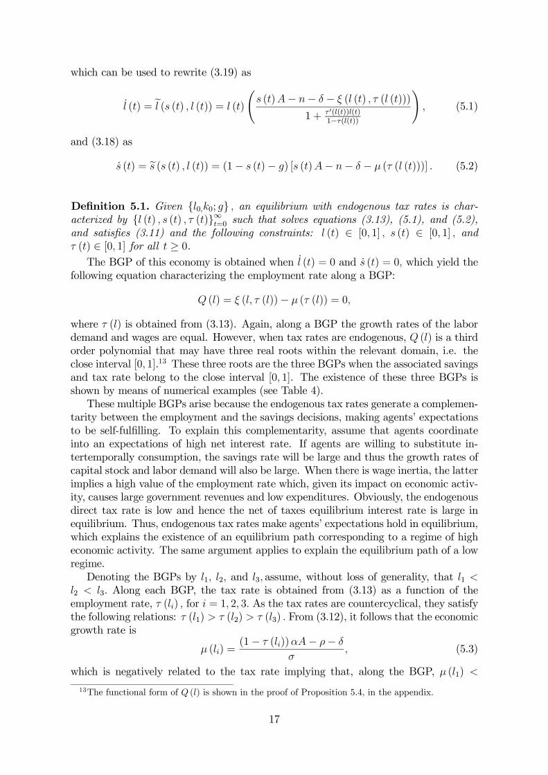
where τ (l) is obtained from (3.13). Again, along a BGP the growth rates of the labordemand and wages are equal. However, when tax rates are endogenous, Q (l) is a thirdorder polynomial that may have three real roots within the relevant domain, i.e. theclose interval [0, 1].13 These three roots are the three BGPs when the associated savingsand tax rate belong to the close interval [0, 1]. The existence of these three BGPs isshown by means of numerical examples (see Table 4).These multiple BGPs arise because the endogenous tax rates generate a complemen-

tarity between the employment and the savings decisions, making agents’ expectationsto be self-fulfilling. To explain this complementarity, assume that agents coordinateinto an expectations of high net interest rate. If agents are willing to substitute in-tertemporally consumption, the savings rate will be large and thus the growth rates ofcapital stock and labor demand will also be large. When there is wage inertia, the latterimplies a high value of the employment rate which, given its impact on economic activ-ity, causes large government revenues and low expenditures. Obviously, the endogenousdirect tax rate is low and hence the net of taxes equilibrium interest rate is large inequilibrium. Thus, endogenous tax rates make agents’ expectations hold in equilibrium,which explains the existence of an equilibrium path corresponding to a regime of higheconomic activity. The same argument applies to explain the equilibrium path of a lowregime.Denoting the BGPs by l1, l2, and l3, assume, without loss of generality, that l1 <

l2 < l3. Along each BGP, the tax rate is obtained from (3.13) as a function of theemployment rate, τ (li) , for i = 1, 2, 3. As the tax rates are countercyclical, they satisfythe following relations: τ (l1) > τ (l2) > τ (l3) . From (3.12), it follows that the economicgrowth rate is

µ (li) =(1− τ (li))αA− ρ− δ

σ, (5.3)

which is negatively related to the tax rate implying that, along the BGP, µ (l1) <

13The functional form of Q (l) is shown in the proof of Proposition 5.4, in the appendix.

17

µ (l2) < µ (l3) . Finally, the savings rate is obtained from s (t) = 0

s (li) =µ (li) + n+ δ

A.

Because the savings rate is positively related with economic growth, the following re-lations hold: s (l1) < s (l2) < s (l3) . Thus, it follows that BGP 1 (i.e. l1, τ (l1) , µ (l1) ,s (l1)) corresponds to a regime of low economic activity and high tax rates, whereasBGP 3 (i.e. l3, τ (l3) , µ (l3) , s (l3)) corresponds to a regime of high economic activityand low tax rates.Analogously to the US case, the countercyclical behavior of the direct tax rate in

Spain is associated with our scenario of endogenous tax rates which, together with therelevant values (see Table 4), characterizes the Spanish economy in the long-run. SinceBGP 2 is unstable, we identify BGP 1 with the low regime of the Spanish economy andBGP 3 with the high regime. As Table 4 shows, the model is able to replicate fairlywell the two regimes.

[Insert Table 4]

In what follows we look at the effects of the parameters along BGPs 1 and 3, andthen characterize the stability of each BGP.

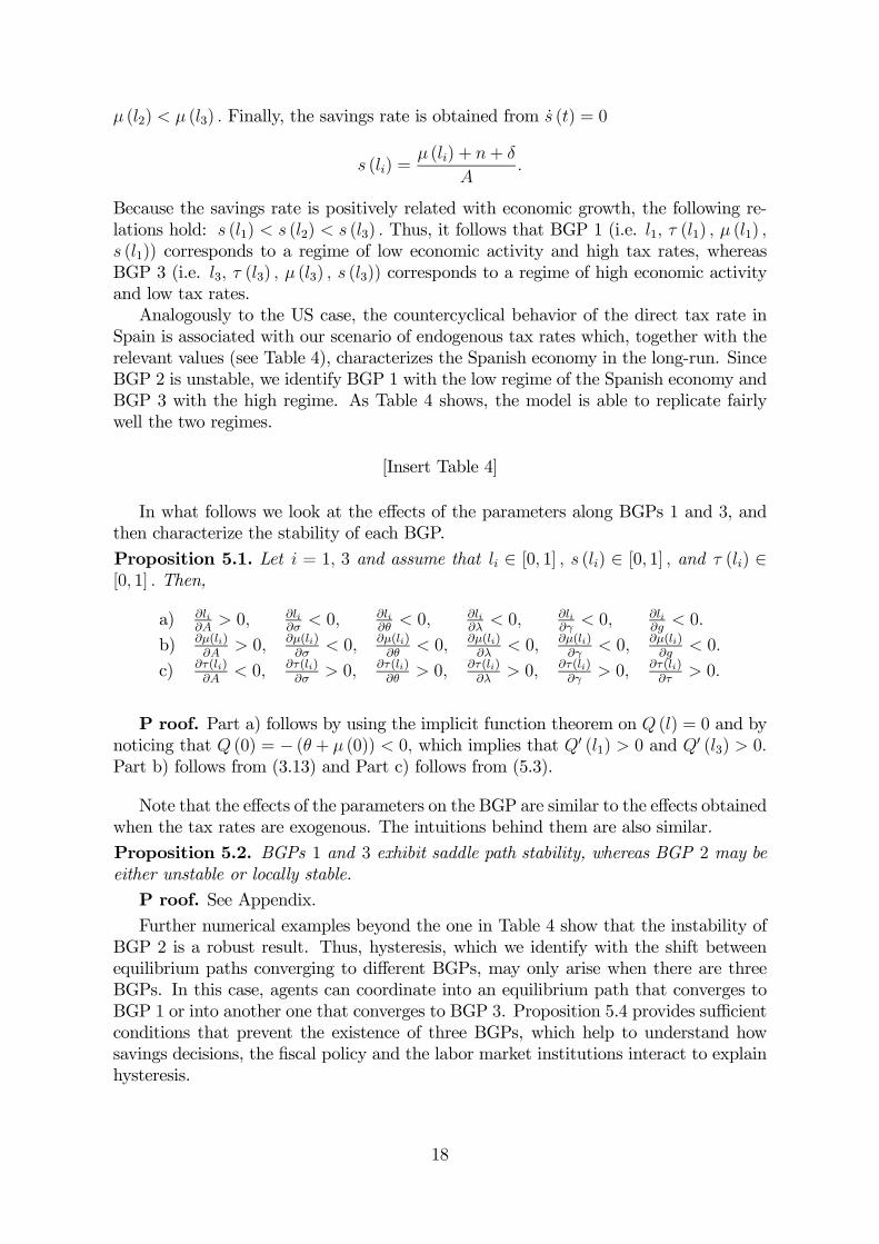
Proposition 5.1. Let i = 1, 3 and assume that li ∈ [0, 1] , s (li) ∈ [0, 1] , and τ (li) ∈[0, 1] . Then,

a) ∂li∂A

> 0, ∂li∂σ

< 0, ∂li∂θ

< 0, ∂li∂λ

< 0, ∂li∂γ

< 0, ∂li∂g

< 0.

b) ∂µ(li)∂A

> 0, ∂µ(li)∂σ

< 0, ∂µ(li)∂θ

< 0, ∂µ(li)∂λ

< 0, ∂µ(li)∂γ

< 0, ∂µ(li)∂g

< 0.

c) ∂τ(li)∂A

< 0, ∂τ(li)∂σ

> 0, ∂τ(li)∂θ

> 0, ∂τ(li)∂λ

> 0, ∂τ(li)∂γ

> 0, ∂τ(li)∂τ

> 0.

P roof. Part a) follows by using the implicit function theorem on Q (l) = 0 and bynoticing that Q (0) = − (θ + µ (0)) < 0, which implies that Q0 (l1) > 0 and Q0 (l3) > 0.Part b) follows from (3.13) and Part c) follows from (5.3).

Note that the effects of the parameters on the BGP are similar to the effects obtainedwhen the tax rates are exogenous. The intuitions behind them are also similar.

Proposition 5.2. BGPs 1 and 3 exhibit saddle path stability, whereas BGP 2 may beeither unstable or locally stable.

P roof. See Appendix.Further numerical examples beyond the one in Table 4 show that the instability of

BGP 2 is a robust result. Thus, hysteresis, which we identify with the shift betweenequilibrium paths converging to different BGPs, may only arise when there are threeBGPs. In this case, agents can coordinate into an equilibrium path that converges toBGP 1 or into another one that converges to BGP 3. Proposition 5.4 provides sufficientconditions that prevent the existence of three BGPs, which help to understand howsavings decisions, the fiscal policy and the labor market institutions interact to explainhysteresis.

18

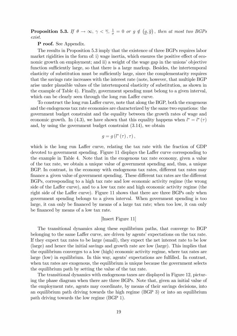
Proposition 5.3. If θ → ∞, γ < γ, 1σ= 0 or g /∈ ¡g, g¢ , then at most two BGPs

exist.P roof. See Appendix.The results in Proposition 5.3 imply that the existence of three BGPs requires labor

market rigidities in the form of: i) wage inertia, which ensures the positive effect of eco-nomic growth on employment; and ii) a weight of the wage gap in the unions’ objectivefunction sufficiently large, so that there is a large markup. Besides, the intertemporalelasticity of substitution must be sufficiently large, since the complementarity requiresthat the savings rate increases with the interest rate (note, however, that multiple BGParise under plausible values of the intertemporal elasticity of substitution, as shown inthe example of Table 4). Finally, government spending must belong to a given interval,which can be clearly seen through the long run Laffer curve.To construct the long run Laffer curve, note that along the BGP, both the exogenous

and the endogenous tax rate economies are characterized by the same two equations: thegovernment budget constraint and the equality between the growth rates of wage andeconomic growth. In (4.3), we have shown that this equality happens when l∗ = l∗ (τ)and, by using the government budget constraint (3.14), we obtain

g = g (l∗ (τ) , τ) ,

which is the long run Laffer curve, relating the tax rate with the fraction of GDPdevoted to government spending. Figure 11 displays the Laffer curve corresponding tothe example in Table 4. Note that in the exogenous tax rate economy, given a valueof the tax rate, we obtain a unique value of government spending and, thus, a uniqueBGP. In contrast, in the economy with endogenous tax rates, different tax rates mayfinance a given value of government spending. These different tax rates are the differentBGPs, corresponding to a high tax rate and low economic activity regime (the wrongside of the Laffer curve), and to a low tax rate and high economic activity regime (theright side of the Laffer curve). Figure 11 shows that there are three BGPs only whengovernment spending belongs to a given interval. When government spending is toolarge, it can only be financed by means of a large tax rate; when too low, it can onlybe financed by means of a low tax rate.

[Insert Figure 11]

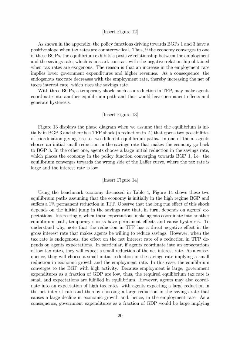
The transitional dynamics along these equilibrium paths, that converge to BGPbelonging to the same Laffer curve, are driven by agents’ expectations on the tax rate.If they expect tax rates to be large (small), they expect the net interest rate to be low(large) and hence the initial savings and growth rate are low (large). This implies thatthe equilibrium converges to a low (high) economic activity regime, where tax rates arelarge (low) in equilibrium. In this way, agents’ expectations are fulfilled. In contrast,when tax rates are exogenous, the equilibrium is unique because the government selectsthe equilibrium path by setting the value of the tax rate.The transitional dynamics with endogenous taxes are displayed in Figure 12, pictur-

ing the phase diagram when there are three BGPs. Note that, given an initial value ofthe employment rate, agents may coordinate, by means of their savings decisions, intoan equilibrium path driving towards the high regime (BGP 3) or into an equilibriumpath driving towards the low regime (BGP 1).

19

[Insert Figure 12]

As shown in the appendix, the policy functions driving towards BGPs 1 and 3 have apositive slope when tax rates are countercyclical. Thus, if the economy converges to oneof these BGPs, the equilibrium exhibits a positive relationship between the employmentand the savings rate, which is in stark contrast with the negative relationship obtainedwhen tax rates are exogenous. The reason is that an increase in the employment rateimplies lower government expenditures and higher revenues. As a consequence, theendogenous tax rate decreases with the employment rate, thereby increasing the net oftaxes interest rate, which rises the savings rate.With three BGPs, a temporary shock, such as a reduction in TFP, may make agents

coordinate into another equilibrium path and thus would have permanent effects andgenerate hysteresis.

[Insert Figure 13]

Figure 13 displays the phase diagram when we assume that the equilibrium is ini-tially in BGP 3 and there is a TFP shock (a reduction in A) that opens two possibilitiesof coordination giving rise to two different equilibrium paths. In one of them, agentschoose an initial small reduction in the savings rate that makes the economy go backto BGP 3. In the other one, agents choose a large initial reduction in the savings rate,which places the economy in the policy function converging towards BGP 1, i.e. theequilibrium converges towards the wrong side of the Laffer curve, where the tax rate islarge and the interest rate is low.

[Insert Figure 14]

Using the benchmark economy discussed in Table 4, Figure 14 shows these twoequilibrium paths assuming that the economy is initially in the high regime BGP andsuffers a 1% permanent reduction in TFP. Observe that the long run effect of this shockdepends on the initial jump in the savings rate that, in turn, depends on agents’ ex-pectations. Interestingly, when these expectations make agents coordinate into anotherequilibrium path, temporary shocks have permanent effects and cause hysteresis. Tounderstand why, note that the reduction in TFP has a direct negative effect in thegross interest rate that makes agents be willing to reduce savings. However, when thetax rate is endogenous, the effect on the net interest rate of a reduction in TFP de-pends on agents expectations. In particular, if agents coordinate into an expectationsof low tax rates, they will expect a small reduction of the net interest rate. As a conse-quence, they will choose a small initial reduction in the savings rate implying a smallreduction in economic growth and the employment rate. In this case, the equilibriumconverges to the BGP with high activity. Because employment is large, governmentexpenditures as a fraction of GDP are low, thus, the required equilibrium tax rate issmall and expectations are fulfilled in equilibrium. However, agents may also coordi-nate into an expectation of high tax rates, with agents expecting a large reduction inthe net interest rate and thereby choosing a large reduction in the savings rate thatcauses a large decline in economic growth and, hence, in the employment rate. As aconsequence, government expenditures as a fraction of GDP would be large implying

20

a large equilibrium tax rate. In this equilibrium, expectations are fulfilled again, butnow a temporary reduction in TFP has permanent effects.Finally, according to our model, the different economic performance of the US and

the European countries after the temporary shocks of the 1970’s can be explained by adifferent response in terms of fiscal policies. In the US, direct tax rates were kept con-stant, and employment and growth suffered a temporary decline. In Europe, tax ratesexhibited a countercyclical behavior and employment and growth suffered a persistentdecline. The model explains this persistent decline as a result of a coordination intoanother equilibrium path.

6. Concluding remarks

We have used a growth model with a non-competitive labor market to show that endoge-nous tax rates generate complementarities between employment and capital yielding thepossibility of multiple equilibria. With multiple equilibria, the equilibrium path is theresult of a coordination among equilibria with high tax rates and low employment andsavings rates; and equilibria with low tax rates and high economic activity. These equi-librium paths converge to different long run equilibria that belong to opposite sides ofthe Laffer curve.When tax rates are endogenous, agents may coordinate on either side of the Laffer

curve. This coordination failure causes economic instability and, furthermore, agentsmay coordinate into an equilibrium path that converges to the wrong side of the Laffercurve (the low regime). In contrast, when tax rates are exogenous, the governmentselects the equilibrium path setting the value of the tax rate. In this way, the governmentprevents economic instability and may place the economy in an equilibrium path thatconverges to the right side of the Laffer curve. Thus, according to this model, to setthe value of the tax rate is a superior fiscal policy.The model also nests an interpretation of the different performance of the US and

the European economies in the aftermath of temporary shocks such as those occurredin the 1970’s. In particular, we find a correspondence between the acyclical behaviordisplayed by the direct tax rates in the US with our scenario of exogenous tax rates,and their countercyclical behavior in most of the European countries with our scenarioof endogenous tax rates. In response to a temporary reduction in TFP, in the first casethe model implies a temporary decline in the employment, savings and growth rates,which matches well with the US experience. In the second case, the model predicts thepossibility of hysteresis, which also fits the extremely persistent reduction in the pathof employment, growth and saving rates occurred in Europe. The model explains thispermanent reduction as a coordination of agents into an equilibrium with high tax ratesand low employment and savings rates.

21

References

[1] Akram, Q.F. (1998): “Has the unemployment switched between multiple equilib-ria?”, Norges Bank Working Paper no 1998/02.

[2] Akram, Q.F. (1999): “Multiple unemployment equilibria: Do transitory shockshave permanent effects?”, Norges Bank Working Paper no199/06.

[3] Basu, S. and Fernald, J. (1997): “Returns to Scale im U.S. Production: Estimatesand Implications”, Journal of Political Economy, 105, 249-83.

[4] Blanchard, O.J. and L. Summers (1986a), “Hysteresis and the European Unem-ployment Problem,” NBER Macroeconomics Annual, Vol. 1, Cambridge, Mass:MIT Press, p. 15-71.

[5] Blanchard, O.J. and L. Summers (1986b), “Fiscal Increasing Returns, Hysteresis,Real Wages and Unemployment,” NBER Working Paper no 2034.

[6] Blanchard, O.J. and L.H. Summers (1988): “Beyond the Natural Rate Hypothe-sis”, American Economic Review Papers and Proceedings, Vol. 78, 2, p. 182-187.

[7] Blanchard, O.J. and J. Wolfers (2000): “The Role of Shocks and Institutions in theRise of European Unemployment: The Aggregate Evidence”, Economic Journal,Vol. 110, 462, March, C1-C33.

[8] Bianchi, M. and G. Zoega (1998): “Unemployment Persistence: Does the size ofthe shock matter?”, Journal of Applied Econometrics, Vol. 13, No. 3, 283-304.

[9] Buti, M., D. Franco and H. Ongena (1997): “Budgetary Policies during Recessions:Retrospective Application of the Stability and Growth Pact to the Post-War Pe-riod”, Recherches Economiques de Louvain, v. 63, iss. 4, pp. 321-66.

[10] Coimbra, R., T. Lloyd-Braga and L. Modesto (2000): “Unions, Increasing Returnsand Endogenous Fluctuations”, IZA Discussion Paper, no 229, December.

[11] Cross, R. (1988): Unemployment, Hysteresis and the Natural Rate Hypotheses,Blackwell: Oxford.

[12] Cross, R. (1995): The Natural Rate of Unemployment: reflections of 25 years ofhypothesis, Cambridge: Cambridge University Press.

[13] Den Haan, W. (2003): “Temporary Shocks and Unavoidable Transitions to a High-Unemployment Regime, CEPR Discussion Papers, 3704.

[14] Diamond, P. (1982): “Aggregate Demand Management in Search Equilibrium”,Journal of Political Economy, 90, p. 881-894.

[15] Fatás, A. and I. Mihov (2001): “Fiscal Policy and Business Cycles: An EmpiricalInvestigation”, Moneda y Crédito, 212, pp. 167-210.

[16] Garofalo, G.A. and S. Yamarik (2002): “Regional Evidence from a New State-By-State Capital Stock Series”, The Review of Economics and Statistics, 84(2), pp.316-323.

22

[17] Henry, B., M. Karanassou and D.J. Snower (2000): “Adjustment Dynamics andthe Natural Rate: An Account of UK Unemployment”, Oxford Economic Papers,52, 178-203.

[18] Hughes Hallet, A.J. and L. Piscitelli (2002): “Testing for hysteresis against non-linear alternatives”, Journal of Economic Dynamics & Control, 27, p. 303-327.

[19] Jaeger, A. and M. Parkinson (1994): “Some Evidence on Hysteresis in Unemploy-ment Rates”, European Economic Review, 38, p. 329-342.

[20] Karanassou, M. and D.J. Snower (2002): “Unemployment Invariance”, IZA Dis-cussion Paper no o 530.

[21] Karanassou, M., H. Sala and D. Snower (2003): “Unemployment in the EuropeanUnion: A Dynamic Reappraisal”, Economic Modelling, 20, p. 237-273.

[22] Layard, P.R.J., S.J. Nickell and R. Jackman (1991): Unemployment: Macroeco-nomic Performance and the Labor Market, Oxford: Oxford University Press.

[23] León-Ledesma, M. and P. McAdam (2003): “Unemployment, hysteresis and tran-sition”, European Central Bank Working Paper Series No o 234, May.

[24] Lindbeck, A. and D.J. Snower (2001): “Insiders versus Outsiders”, Journal ofEconomic Perspectives, Vol. 15(1), Winter, pp. 165-188.

[25] Manning, A. (1990): “Imperfect competition, multiple equilibria and unemploy-ment policy”, The Economic Journal, Vol. 100, 400, p. 151-162.

[26] Manning, A. (1992): “Multiple equilibria in the British labor market: some em-pirical evidence”, European Economic Review, Vol. 36, 7, October, p. 1.333-1.365.

[27] Mortensen, D.T. (1989): “The persistence and indeterminancy of unemploymentin search equilibrium”, Scandinavian Journal of Economics, 91, p.347-370.

[28] Ortigueira, S. (2003): “Unemployment Benefits and the Persistence of EuropeanUnemployment”,WP series, no27 of Computing in Economics and Finance, Soci-ety for Computational Economics.

[29] Piscitelli, L., R. Cross, M. Grinfeld and H. Lamba (2000): “A test for stronghysteresis”, Computational Economics, 15 (1-2), 59-78.

[30] Rocheteau, G. (1999): “Balanced-budget rules and indeterminacy of the equilib-rium unemployment rate”, Oxford Economic Papers, 51, 399-409.

[31] Rowthorn, R. (1999): “Unemployment, wage bargaining and capital-labor substi-tution”, Cambridge Journal of Economics, 23, p. 413-425.

23

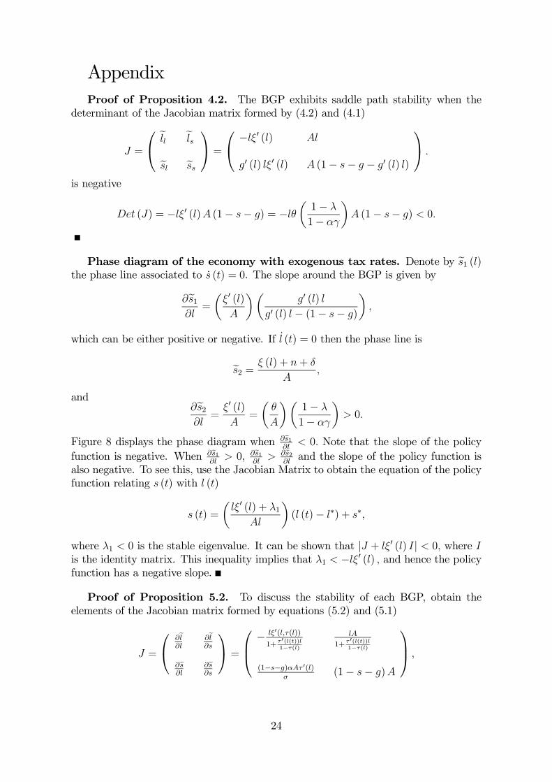
AppendixProof of Proposition 4.2. The BGP exhibits saddle path stability when the

determinant of the Jacobian matrix formed by (4.2) and (4.1)

J =

ell elsesl ess

=

−lξ0 (l) Al

g0 (l) lξ0 (l) A (1− s− g − g0 (l) l)

.

is negative

Det (J) = −lξ0 (l)A (1− s− g) = −lθµ1− λ

1− αγ

¶A (1− s− g) < 0.

Phase diagram of the economy with exogenous tax rates. Denote by es1 (l)the phase line associated to s (t) = 0. The slope around the BGP is given by

∂es1∂l

=

µξ0 (l)A

¶µg0 (l) l

g0 (l) l − (1− s− g)

¶,

which can be either positive or negative. If l (t) = 0 then the phase line is

es2 = ξ (l) + n+ δ

A,

and∂es2∂l

=ξ0 (l)A

=

µθ

A

¶µ1− λ

1− αγ

¶> 0.

Figure 8 displays the phase diagram when ∂es1∂l

< 0. Note that the slope of the policyfunction is negative. When ∂es1

∂l> 0, ∂es1

∂l> ∂es2

∂land the slope of the policy function is

also negative. To see this, use the Jacobian Matrix to obtain the equation of the policyfunction relating s (t) with l (t)

s (t) =

µlξ0 (l) + λ1

Al

¶(l (t)− l∗) + s∗,

where λ1 < 0 is the stable eigenvalue. It can be shown that |J + lξ0 (l) I| < 0, where Iis the identity matrix. This inequality implies that λ1 < −lξ0 (l) , and hence the policyfunction has a negative slope.

Proof of Proposition 5.2. To discuss the stability of each BGP, obtain theelements of the Jacobian matrix formed by equations (5.2) and (5.1)

J =

∂el∂l

∂el∂s

∂es∂l

∂es∂s

=

−lξ0(l,τ(l))1+ τ 0(l(t))l

1−τ(l)

lA

1+ τ 0(l(t))l1−τ(l)

(1−s−g)αAτ 0(l)σ

(1− s− g)A

,

24

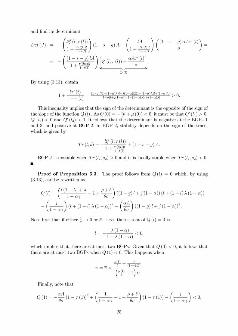
and find its determinant

Det (J) = −Ãlξ0 (l, τ (l))

1 + τ 0(l(t))l1−τ(l)

!(1− s− g)A−

ÃlA

1 + τ 0(l(t))l1−τ(l)

!µ(1− s− g)αAτ 0 (l)

σ

¶=

= −Ã(1− s− g) lA

1 + τ 0(l(t))l1−τ(l)

!·ξ0 (l, τ (l)) +

αAτ 0 (l)σ

¸| {z }

Q0(l)

.

By using (3.13), obtain

1 +lτ 0 (t)1− τ (t)

= (1−g)l(1−(1−α)λ)l+j(1−α)[2(1−(1−α)λ)l+(1−α)λ][(1−g)l+j(1−α)][(1−(1−α)λ)l+(1−α)λ] > 0.

This inequality implies that the sign of the determinant is the opposite of the sign ofthe slope of the functionQ (l) . As Q (0) = − (θ + µ (0)) < 0, it must be that Q0 (l1) > 0,Q0 (l2) < 0 and Q0 (l3) > 0. It follows that the determinant is negative at the BGPs 1and 3, and positive at BGP 2. In BGP 2, stability depends on the sign of the trace,which is given by

Tr (l, s) = − lξ0 (l, τ (l))

1 + τ 0(l(t))l1−τ(l)

+ (1− s− g)A.

BGP 2 is unstable when Tr (l2, s2) > 0 and it is locally stable when Tr (l2, s2) < 0.

Proof of Proposition 5.3. The proof follows from Q (l) = 0 which, by using(3.13), can be rewritten as

Q (l) =

µl (1− λ) + λ

1− αγ− 1 + ρ+ δ

θσ

¶((1− g) l + j (1− α)) (l + (1− l)λ (1− α))

−µ

j

1− αγ

¶(l + (1− l)λ (1− α))2 −

µαA

θσ

¶((1− g) l + j (1− α))2 .

Note first that if either 1σ→ 0 or θ →∞, then a root of Q (l) = 0 is

l = − λ (1− α)

1− λ (1− α)< 0,

which implies that there are at most two BGPs. Given that Q (0) < 0, it follows thatthere are at most two BGPs when Q (1) < 0. This happens when

γ = γ <

µ(1)θ+ j

(1−τ(1))³µ(1)θ+ 1´α.

Finally, note that

Q (1) = −αAθσ(1− τ (1))2 +

µ1

1− αγ− 1 + ρ+ δ

θσ

¶(1− τ (1))−

µj

1− αγ

¶< 0,

25

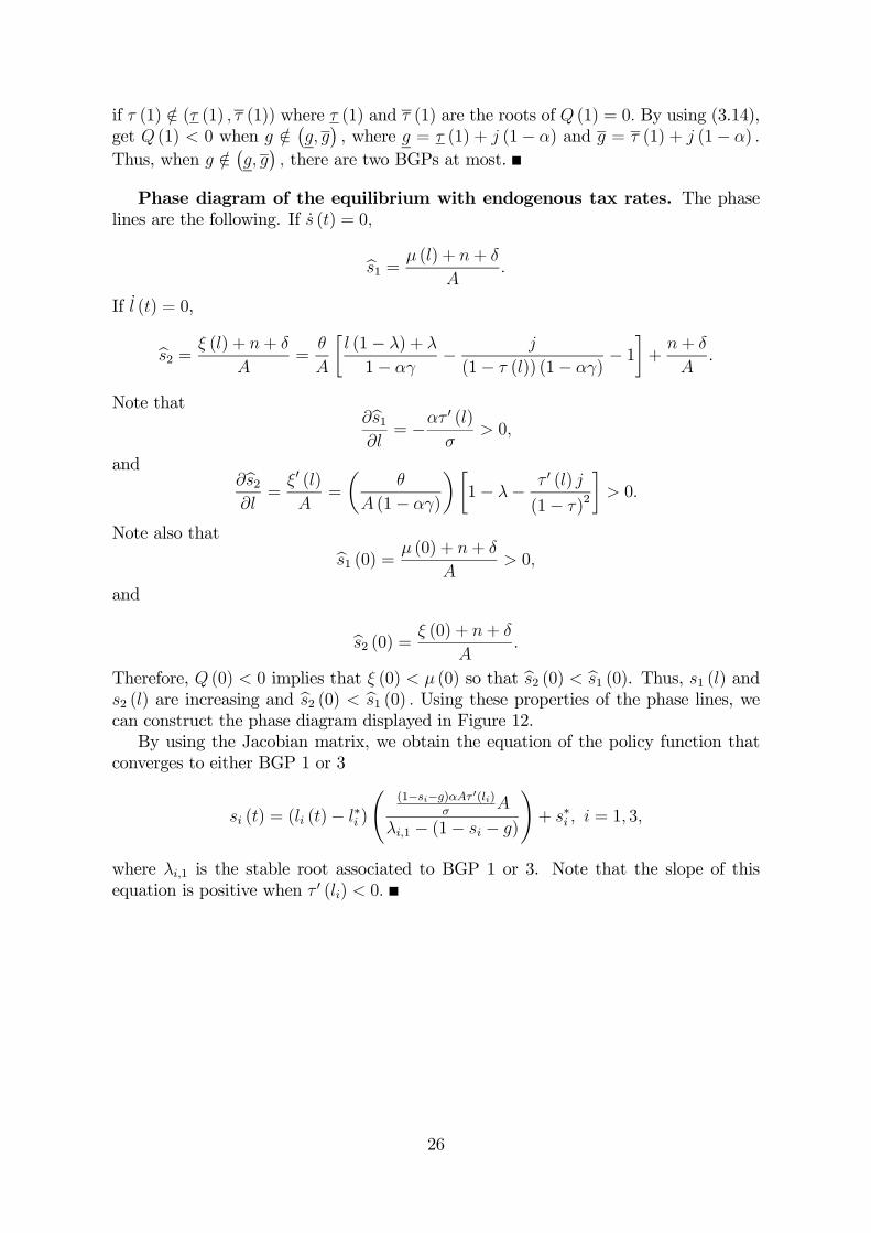
if τ (1) /∈ (τ (1) , τ (1)) where τ (1) and τ (1) are the roots of Q (1) = 0. By using (3.14),get Q (1) < 0 when g /∈ ¡g, g¢ , where g = τ (1) + j (1− α) and g = τ (1) + j (1− α) .

Thus, when g /∈ ¡g, g¢ , there are two BGPs at most.Phase diagram of the equilibrium with endogenous tax rates. The phase

lines are the following. If s (t) = 0,

bs1 = µ (l) + n+ δ

A.

If l (t) = 0,

bs2 = ξ (l) + n+ δ

A=

θ

A

·l (1− λ) + λ

1− αγ− j

(1− τ (l)) (1− αγ)− 1¸+

n+ δ

A.

Note that∂bs1∂l

= −ατ0 (l)σ

> 0,

and∂bs2∂l

=ξ0 (l)A

=

µθ

A (1− αγ)

¶·1− λ− τ 0 (l) j

(1− τ)2

¸> 0.

Note also that bs1 (0) = µ (0) + n+ δ

A> 0,

and

bs2 (0) = ξ (0) + n+ δ

A.

Therefore, Q (0) < 0 implies that ξ (0) < µ (0) so that bs2 (0) < bs1 (0). Thus, s1 (l) ands2 (l) are increasing and bs2 (0) < bs1 (0) . Using these properties of the phase lines, wecan construct the phase diagram displayed in Figure 12.By using the Jacobian matrix, we obtain the equation of the policy function that

converges to either BGP 1 or 3

si (t) = (li (t)− l∗i )

Ã(1−si−g)αAτ 0(li)

σA

λi,1 − (1− si − g)

!+ s∗i , i = 1, 3,

where λi,1 is the stable root associated to BGP 1 or 3. Note that the slope of thisequation is positive when τ 0 (li) < 0.

26

Tables

Table 1: Regimes in the European capital stock growth rates. 1960-1999.Means in annual growth rates expressed in percentage points

Regime 1 Regime 2Means Years Means Years

Austria 7.0 1961-77 4.2 1978-99Belgium 4.4 1961-78 2.8 1979-99Denmark 5.2 1961-74 3.2 1975-99Germany 6.1 1964-71 3.0 1972-99Finland 2.9 1970-99France 4.3 1963-77 2.4 1978-99Italy 4.8 1961-74 3.0 1975-99Netherlands 2.3 1969-99Spain 11.2 1964-75 4.3 1976-99Sweden 4.7 1966-76 2.4 1977-99United Kingdom 1.7 1963-99

Table 2: Covariation in the direct tax rate and the business cycle..

Based on the regression: τ δt = α+ β∆ytwhere τd is the ratio direct taxes

GDP and ∆y is GDP growth

β t-stat. period β t-stat. periodAustria -0.37 -3.72∗ 1964-99 Italy -1.14 -4.84∗ 1961-99Belgium -0.56 -3.15∗ 1970-99 Netherlands -0.31 -2.73∗ 1969-99Denmark -1.04 -2.87∗ 1961-99 Spain -0.56 -2.73∗ 1964-99Germany -0.10 -1.79∗∗ 1961-99 Sweden -0.44 -2.70∗ 1961-99Finland -0.19 -1.92∗∗ 1970-99 UK -0.02 -0.10∗∗∗ 1963-99France -0.45 -3.49∗ 1964-99 US -0.01 -0.14∗∗∗ 1961-99Note: * stands for significant at 1% *** stands for non-significant

** stands for significant between 5% and 10%

27

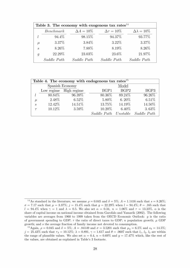
Table 3. The economy with exogenous tax rates14

Benchmark ∆A = 10% ∆τ = 10% ∆λ = 10%

l 94.4% 98.15% 94.37% 93.77%

µ 3.37% 3.84% 3.22% 3.37%

s 8.26% 7.88% 8.19% 8.26%

g 22.29% 23.03% 23.6% 21.97%

Saddle Path Saddle Path Saddle Path Saddle Path

Table 4. The economy with endogenous tax rates15

Spanish Economy ModelLow regime High regime BGP1 BGP2 BGP3

l 80.84% 96.39% 80.36% 89.24% 96.26%µ 2.48% 6.52% 5.80% 6. 20% 6.51%s 12.42% 14.51% 13.75% 14.19% 14.50%τ 10.12% 3.59% 10.20% 6.40% 3. 63%

Saddle Path Unstable Saddle Path

14As standard in the literature, we assume ρ = 0.045 and δ = 5%; A = 1.1416 such that s = 8.26%;σ = 7.17 such that µ = 3.37%; j = 15.4% such that g = 22.29% when l = 94.4%; θ = .165 such thatl = 94.4% when γ = 1 and λ = 0.5. We also set α = 0.34, n = 1.06% and τ = 13.23%. α is theshare of capital income on national income obtained from Garofalo and Yamarik (2002). The followingvariables are averages from 1960 to 1999 taken from the OECD Economic Outlook: g is the ratioof government spending to GDP; τ the ratio of direct taxes to GDP; n population growth; µ GDPgrowth; and s the average fraction of family income not devoted to consumption.15Again, ρ = 0.045 and δ = 5%; A = .84149 and σ = 3.5201 such that µ3 = 6.5% and s3 = 14.5%;

j = 25.43% such that τ3 = 10.12%; λ = 0.891, γ = 1.617 and θ = .0607 such that l1, l2, l3 are withinthe range of plausible values. We also set α = 0.4, n = 0.69% and g = 17.47% which, like the rest ofthe values, are obtained as explained in Table’s 3 footnote.

28

Figures

0

2

4

6

8

10

12

60 65 70 75 80 85 90 95

a. European unemployment rate

Low regime

High regime

0

2

4

6

8

10

12

60 65 70 75 80 85 90 95

b. US unemployment rate

Uniqueregime

0.00

0.02

0.04

0.06

0.08

0.10

0.12

0 2 4 6 8 10 12 14

Kernel Density (Normal, h = 1.3485)

Low regime mean at 2.54%

Change of regime at 6.22%

High regimemean at 9.69%

c. Kernel density analysis of the European unemployment rate

0.00

0.05

0.10

0.15

0.20

0.25

0.30

4 6 8 10



Change ofregime at 9.03%


d. Kernel density analysis of the US unemployment rate

Figure 1. Unemployment in Europe and the US

29

0

1

2

3

4

5

6

60 65 70 75 80 85 90 95

Austria

0

2

4

6

8

10

12

60 65 70 75 80 85 90 95

Belgium

0

2

4

6

8

10

12

60 65 70 75 80 85 90 95

Denmark

0.00

0.02

0.04

0.06

0.08

0.10

60 65 70 75 80 85 90 95

Germany

0

4

8

12

16

20

60 65 70 75 80 85 90 95

Finland

0

2

4

6

8

10

12

14

60 65 70 75 80 85 90 95

France

2

4

6

8

10

12

14

60 65 70 75 80 85 90 95

Italy

0

2

4

6

8

10

12

60 65 70 75 80 85 90 95

Netherlands

0

5

10

15

20

25

60 65 70 75 80 85 90 95

Spain

0

2

4

6

8

10

60 65 70 75 80 85 90 95

Sweden

0

2

4

6

8

10

12

60 65 70 75 80 85 90 95

United Kingdom

Figure 2. Unemployment rate: actual series and regime means in European countries

30

0.00

0.05

0.10

0.15

0.20

0.25

0.30

0 2 4 6





Austria

0.00

0.02

0.04

0.06

0.08

0.10

0 5 10


Low regimemean at 2.37%



Belgium

0.00

0.02

0.04

0.06

0.08

0.10

0.12

0 2 4 6 8 10 12





Denmark

0.00

0.02

0.04

0.06

0.08

0.10

0.12

-2 0 2 4 6 8 10 12





Germany

0.00

0.02

0.04

0.06

0.08

0.10

0.12

0.14

0 5 10 15





Finland

0.00

0.02

0.04

0.06

0.08

0.10

0 5 10 15





France

0.00

0.04

0.08

0.12

0.16

2 4 6 8 10 12 14





Italy

0.00

0.02

0.04

0.06

0.08

0.10

0.12

0.14

0 2 4 6 8 10 12


Unique regime mean at 5.44%

Netherlands

0.00

0.01

0.02

0.03

0.04

0.05

0.06

0 10 20 30





Spain

0.0

0.1

0.2

0.3

0.4

0.5

2 4 6 8





Sweden

0.00

0.02

0.04

0.06

0.08

0.10

0.12

0 2 4 6 8 10 12 14





United Kingdom

Figure 3. Kernel density analysis of the European countries unemployment rate

31

0.03

0.04

0.05

0.06

0.07

0.08

0.09

60 65 70 75 80 85 90 95

Austria

0.020

0.025

0.030

0.035

0.040

0.045

0.050

0.055

60 65 70 75 80 85 90 95

Belgium

0.01

0.02

0.03

0.04

0.05

0.06

0.07

60 65 70 75 80 85 90 95

Denmark

0.02

0.04

0.06

0.08

0.10

0.12

0.14

0.16

60 65 70 75 80 85 90 95

Germany

-0.01

0.00

0.01

0.02

0.03

0.04

0.05

0.06

60 65 70 75 80 85 90 95

Finland

0.01

0.02

0.03

0.04

0.05

0.06

60 65 70 75 80 85 90 95

France

0.02

0.03

0.04

0.05

0.06

0.07

60 65 70 75 80 85 90 95

Italy

0.00

0.01

0.02

0.03

0.04

0.05

60 65 70 75 80 85 90 95

Netherlands

0.00

0.02

0.04

0.06

0.08

0.10

0.12

0.14

60 65 70 75 80 85 90 95

Spain

0.00

0.01

0.02

0.03

0.04

0.05

0.06

60 65 70 75 80 85 90 95

Sweden

0.005

0.010

0.015

0.020

0.025

0.030

0.035

0.040

60 65 70 75 80 85 90 95

United Kingdom

Figure 4. Capital stock growth rate: actual series and regime means in the European countries

32

0

5

10

15

20

25

30

0.02 0.04 0.06 0.08


Austria




0

10

20

30

40

0.02 0.03 0.04 0.05


Belgium


Low regimemean at2.8%


0

10

20

30

40

0.01 0.02 0.03 0.04 0.05 0.06 0.07


Denmark




0

5

10

15

20

25

30

0.02 0.04 0.06 0.08 0.10 0.12 0.14


Germany




Temporarypick at 14%

0

5

10

15

20

25

0.00 0.02 0.04 0.06


Finland


Temporarylow regimemean at 0.53%


0

10

20

30

40

0.01 0.02 0.03 0.04 0.05 0.06


France




0

10

20

30

40

0.02 0.03 0.04 0.05 0.06 0.07 0.08


Italy




Temporaryvery highregime at 6.7%

0

10

20

30

40

50

60

0.01 0.02 0.03 0.04 0.05


Netherlands

Unique regimeat 2.3%

0

2

4

6

8

10

12

14

0.00 0.05 0.10 0.15


Spain




0

10

20

30

40

0.00 0.01 0.02 0.03 0.04 0.05 0.06


Sweden




0

20

40

60

80

0.01 0.02 0.03 0.04


United Kingdom

Temporaryhigh regimemean at 3.5%



Figure 5. Kernel density analysis of the European countries capital stock growth

33

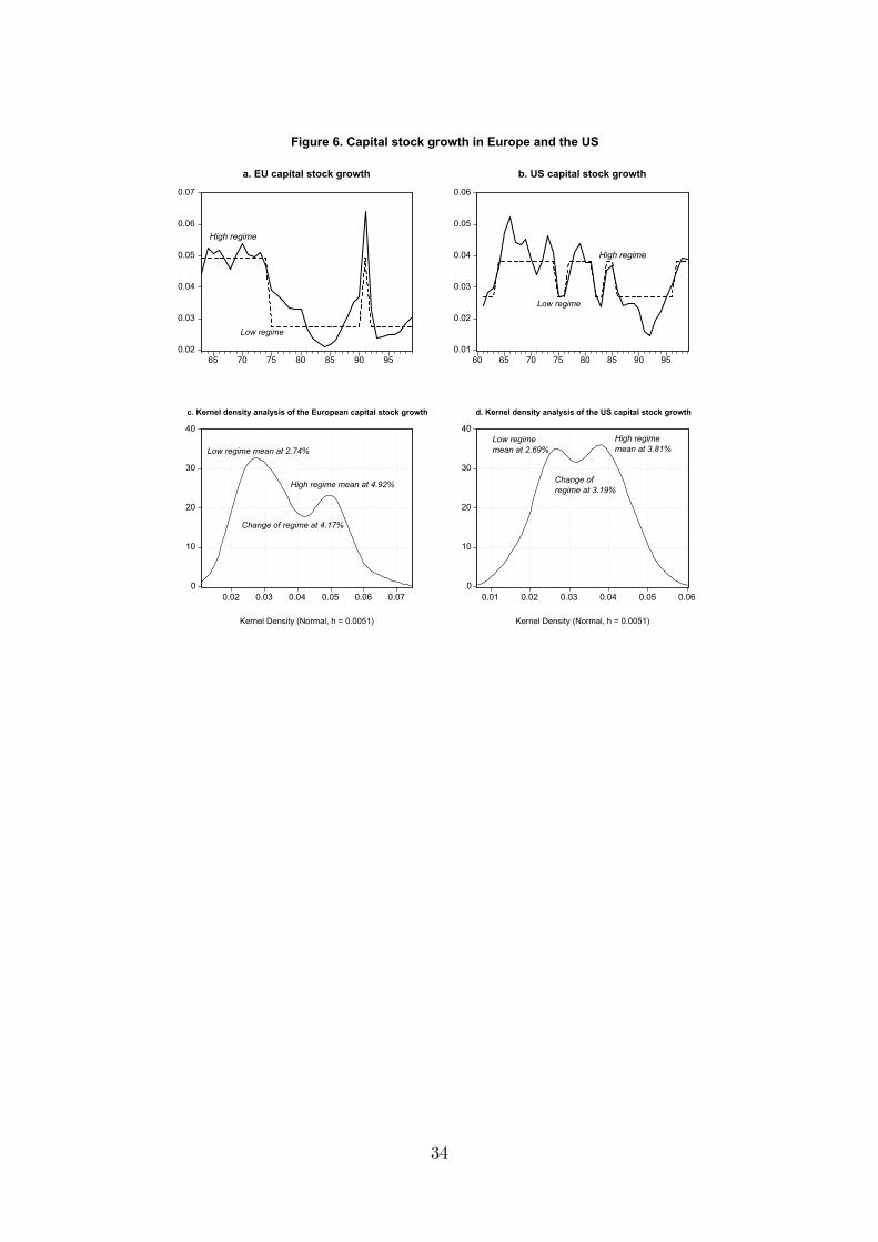
0.02

0.03

0.04

0.05

0.06

0.07

65 70 75 80 85 90 95

a. EU capital stock growth

High regime

Low regime

0.01

0.02

0.03

0.04

0.05

0.06

60 65 70 75 80 85 90 95

b. US capital stock growth

High regime

Low regime

0

10

20

30

40

0.02 0.03 0.04 0.05 0.06 0.07



High regime mean at 4.92%


c. Kernel density analysis of the European capital stock growth

0

10

20

30

40

0.01 0.02 0.03 0.04 0.05 0.06





d. Kernel density analysis of the US capital stock growth

Figure 6. Capital stock growth in Europe and the US

34

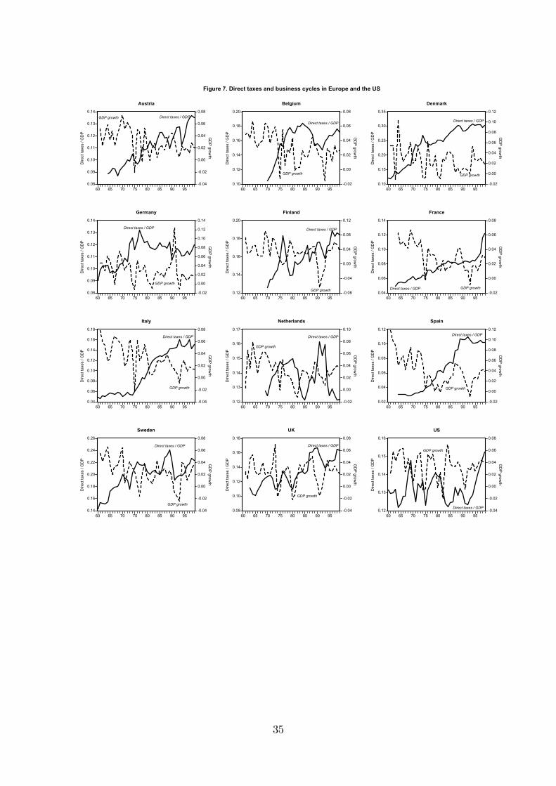
0.08

0.09

0.10

0.11

0.12

0.13

0.14

-0.04

-0.02

0.00

0.02

0.04

0.06

0.08

60 65 70 75 80 85 90 95

Austria

Dire

ct ta

xes

/ GD

P

GD

P growth

Direct taxes / GDPGDP growth

0.10

0.12

0.14

0.16

0.18

0.20

-0.02

0.00

0.02

0.04

0.06

0.08

60 65 70 75 80 85 90 95

Belgium

Dire

ct ta

xes

/ GD

P

GD

P growth

Direct taxes / GDP

GDP growth

0.10

0.15

0.20

0.25

0.30

0.35

-0.02

0.00

0.02

0.04

0.06

0.08

0.10

0.12

60 65 70 75 80 85 90 95

Denmark

Dire

ct ta

xes

/ GD

P

GD

P growth

Direct taxes / GDP

GDP growth

0.08

0.09

0.10

0.11

0.12

0.13

0.14

-0.02

0.00

0.02

0.04

0.06

0.08

0.10

0.12

0.14

60 65 70 75 80 85 90 95

Germany

Dire

ct ta

xes

/ GD

P

GD

P growth

Direct taxes / GDP

GDP growth

0.12

0.14

0.16

0.18

0.20

-0.08

-0.04

0.00

0.04

0.08

0.12

60 65 70 75 80 85 90 95

Finland

Dire

ct ta

xes

/ GD

P

GD

P growth

Direct taxes / GDP

GDP growth 0.04

0.06

0.08

0.10

0.12

0.14

-0.02

0.00

0.02

0.04

0.06

0.08

60 65 70 75 80 85 90 95

France

Dire

ct ta

xes

/ GD

P

GD

P growth

Direct taxes / GDP GDP growth

0.04

0.06

0.08

0.10

0.12

0.14

0.16

0.18

-0.04

-0.02

0.00

0.02

0.04

0.06

0.08

60 65 70 75 80 85 90 95

Italy

Dire

ct ta

xes

/ GD

P

GD

P growth

Direct taxes / GDP

GDP growth

0.12

0.13

0.14

0.15

0.16

0.17

-0.02

0.00

0.02

0.04

0.06

0.08

0.10

60 65 70 75 80 85 90 95

Netherlands

Dire

ct ta

xes

/ GD

P

GD

P growth

Direct taxes / GDP

GDP growth

0.02

0.04

0.06

0.08

0.10

0.12

-0.02

0.00

0.02

0.04

0.06

0.08

0.10

0.12

60 65 70 75 80 85 90 95

Spain

Dire

ct ta

xes

/ GD

P

GD

P growth

Direct taxes / GDP

GDP growth

0.14

0.16

0.18

0.20

0.22

0.24

0.26

-0.04

-0.02

0.00

0.02

0.04

0.06

0.08

60 65 70 75 80 85 90 95

Sweden

Dire

ct ta

xes

/ GD

P

GD

P growth

Direct taxes / GDP

GDP growth

0.08

0.10

0.12

0.14

0.16

0.18

-0.04

-0.02

0.00

0.02

0.04

0.06

0.08

60 65 70 75 80 85 90 95

UK

Dire

ct ta

xes

/ GD

P

GD

P growth

Direct taxes / GDP

GDP growth

0.12

0.13

0.14

0.15

0.16

-0.04

-0.02

0.00

0.02

0.04

0.06

0.08

60 65 70 75 80 85 90 95

US

Dire

ct ta

xes

/ GD

P

GD

P growth

Direct taxes / GDP

GDP growth

Figure 7. Direct taxes and business cycles in Europe and the US

35

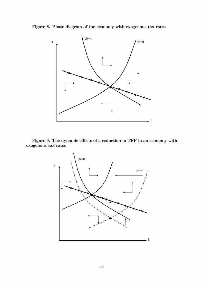
Figure 8. Phase diagram of the economy with exogenous tax rates

s

l

ds=0dl=0

Figure 9. The dynamic effects of a reduction in TFP in an economy withexogenous tax rates

s

l

ds=0

dl=0

36

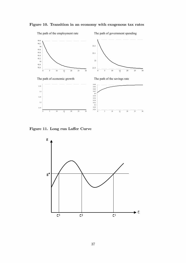
Figure 10. Transition in an economy with exogenous tax rates

The path of the employment rate The path of government spending

t 302520151050

94.4

94.2

94

93.8

93.6

93.4

93.2

93

92.8

92.6

t 302520151050

22.2

22.1

22

21.9

The path of economic growth The path of the savings rate

t 302520151050

3.35

3.3

3.25

3.2

3.15

t 302520151050

8.488.468.448.42

8.48.388.368.348.32

8.38.288.26

Figure 11. Long run Laffer Curve

g

ح

g*

3ح 2ح 1ح

g

ح

g*

3ح 2ح 1ح

37

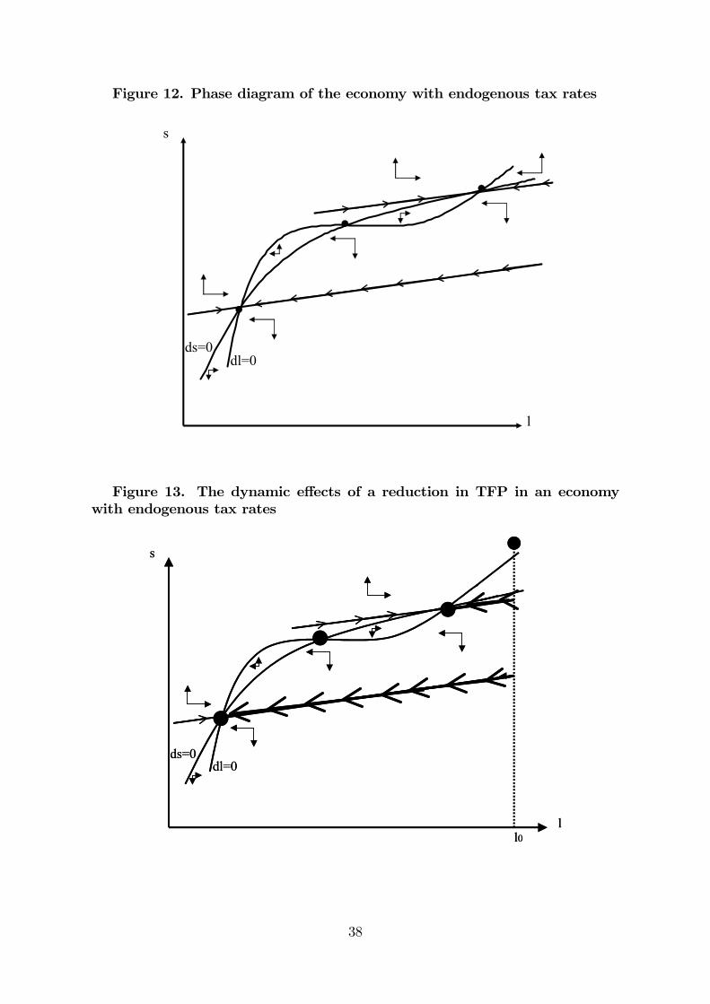
Figure 12. Phase diagram of the economy with endogenous tax rates

s

l

ds=0dl=0

Figure 13. The dynamic effects of a reduction in TFP in an economywith endogenous tax rates

s

l

ds=0dl=0

l0

s

l

ds=0dl=0

l0

38

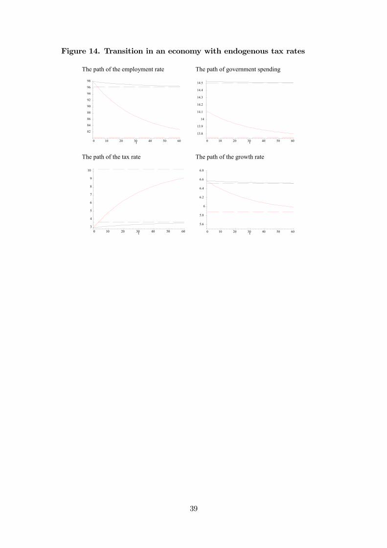
Figure 14. Transition in an economy with endogenous tax rates

The path of the employment rate The path of government spending

t 6050403020100

98

96

94

92

90

88

86

84

82

t 6050403020100

14.5

14.4

14.3

14.2

14.1

14

13.9

13.8

The path of the tax rate The path of the growth rate

t 6050403020100

10

9

8

7

6

5

4

3

t 6050403020100

6.8

6.6

6.4

6.2

6

5.8

5.6

39

TÍTOLNUM AUTOR DATA

Abril 2004Unemployment, growth and fiscal policy: new insights on the hysteresis hypothesis*

04.04 Xavier Raurich, Hector Sala,Valeri Sorolla

Març 2004Polarització comarcal de rendes a Catalunya04.03 Juan Antonio Duro

Març 2004Análisis de agrupaciones provinciales a partir del enfoque de desigualdad y polarización: una nota

04.02 Juan Antonio Duro

Gener 2004Producción, empleo y eficiencia productiva de la empresa española

04.01 Oriol Roca Segalés, Hector Sala Lorda.

Desembre 2003

Subjective Income Expectations, Canonical Models and Income Risk

03.10 Xavier Ramos, Christian Schluter.

Desembre 2003

Es Barcelona una ciudad policéntrica ?03.09 Ivan Muñiz, Anna Galindo, Miguel Angel

Garcia.

Octubre 2003

Does persistence of social exclusion exist in Spain?03.08 Ambra Poggi.

Juny 2003Relating Severe Poverty and Chronic Poverty03.07 Shahin Yaqub

Abril 2003Regional decomposition of CO2 emissions in the world: a cluster analysis

03.06 Vicent Alcántara, Rosa Duarte, Teresa Obis

Abril 2003On the regional impact of public capital formation in spain

03.05 Alfredo Marvao Pereira i Oriol roca Sagalés

Març 2003Demand and revenue implications of an integrated public transport policy. The case of Madrid

03.04 Anna Matas

Març 2003Eficacia y eficiencia de los subsidios asistenciales en la lucha contra la pobreza en España: Una valoración a

partir de EspaSim

03.01 Horacio Levy, Magda Mercader

Febrer 2003Barcelona, Metropolis policentrica en red03.03 Joan Trullén i Rafael Boix

Febrer 2003Factor decomposition of spatial income inequality: a revision

03.02 Juan Antonio Duro

Novembre 2002

Long-run Inflation-Unemployment Dynamics: The Spanish Phillips Curve and Economic Policy

02.11 Marika Karanassou, Hector Sala, Dennis J.

Snower

Documents

Departament d'Economia Aplicada - core.ac.uk · 1. Introduction This paper takes a new look at the hysteresis hypotheses and provides new insights to evaluate the European unemployment