DENGUE MODEL WITH EARLY LIFE STAGE OF VECTORS AND …

c⃝ REVISTA DE MATEMÁTICA: TEORÍA Y APLICACIONES 2020 27(1) : 157–177

CIMPA – UCR ISSN: 1409-2433 (PRINT), 2215-3373 (ONLINE)

DOI: https://doi.org/10.15517/rmta.v27i1.39966

DENGUE MODEL WITH EARLY-LIFE STAGE OF

VECTORS AND AGE-STRUCTURE WITHIN HOST

MODELO DE DENGUE CON ETAPA TEMPRANA

EN VECTORES Y ESTRUCTURA DE EDAD

EN EL HUÉSPED

FABIO SANCHEZ∗ JUAN G. CALVO†

Received: 7/Aug/2019; Revised: 26/Aug/2019;Accepted: 18/Sep/2019

∗University of Costa Rica, CIMPA-School of Mathematics, San José, Costa Rica. E-Mail:[email protected]

†Misma dirección que/Same address as: F. Sánchez. E-Mail: [email protected]

157

158 F. SANCHEZ — J. G. CALVO

Abstract

We construct an epidemic model for the transmission of dengue feverwith an early-life stage in the vector dynamics and age-structure withinhosts. The early-life stage of the vector is modeled via a general func-tion that supports multiple vector densities. The basic reproductive num-ber and vector demographic threshold are computed to study the localand global stability of the infection-free state. A numerical framework isimplemented and simulations are performed.

Keywords: dengue fever; epidemic models; mathematical modeling; vector-borne diseases; age-structured model.

Resumen

Se construye un modelo epidémico para la dinámica de transmisión dela fiebre del dengue con etapa temprana de vida en los vectores y estructurade edad en las clases de los huéspedes. La etapa de vida temprana delvector, se modela a través de una función general que admite múltiplesdensidades de vectores. El número reproductivo básico y vector de umbraldemográfico, se calculan para estudiar la estabilidad local y global delestado libre de infección. Se implementa además un marco numérico y serealizan simulaciones.

Palabras clave: dengue; modelos epidémicos; modelizaje matemático; enfer-medades vectoriales; modelos con estructura de edad.

Mathematics Subject Classification: 93A30, 92B99, 37N25

1 Introduction

Dengue fever has been a burden to public health officials in the tropics and sub-tropics since the 20th century [2, 7]. Dengue virus, of the genus Flavivirus of thefamily Flaviviridae, is an infectious disease transmitted by the mosquitoes Aedesaegypti and Aedes albopictus [6]. There are four serotypes of the dengue virus,called DEN-1, DEN-2, DEN-3, and DEN-4. After infection of one serotype, theinfected person acquires lifelong immunity for that specific serotype and short-term immunity to other serotypes [2].

Rev.Mate.Teor.Aplic. (ISSN print: 1409-2433; online: 2215-3373) Vol. 27(1): 157–177, Jan–Jun 2020

DENGUE MODEL WITH EARLY-LIFE STAGE OF VECTORS . . . 159

There are two stages in the transmission cycle of dengue that have beenreported. There is an enzootic transmission cycle between primates mostly inforests, with transmission between vectors through feeding from infected ani-mals [6]. These infected mosquitoes rarely wander far from the forest, so theinfection to human populations comes from humans or livestock who visit a for-est with presence of the virus, encounter an infected vector, become infected,and then infect the mosquitoes in their population center, which then can spreadthe disease to the rest of the population. In the case of rural, small populations,since the population rapidly gets saturated with the infection and subsequentlyimmunized, the epidemic usually is short-termed. The other stage is betweenvectors and humans, where vectors bite an infected human and can potentiallybecome infected. In this work we will focus on the interaction between vectorsand humans.

The model in [11] focuses on the early-life stage of the vector and exploresthe effect of multiple vector densities on dengue outbreaks. Previous work ondengue models mostly focus on the adult vector-host interactions; see, e.g., [5,3, 4, 12, 8, 9, 1, 10].

The model we present here incorporates age-structure within the host pop-ulation, as well as the early-life stage of the vector as in [11]. The inclusionof age-structure in the human/host population can help to determine preventionand control strategies based on specific population age groups and other socialfactors inherent to a subgroup of the population at risk.

This article is organized as follows. In Section 2, we outline the mathemat-ical model. In Section 3, we compute the vector demographic threshold, thebasic reproductive number, and determine the stability of the system. Section 4includes the numerical scheme and numerical simulations, confirming the theo-retical results. Finally, in Section 5 we present some relevant conclusions andfinal thoughts.

2 Mathematical model

We consider a compartmental model with age-structure within the host popu-lation, with susceptible, infectious and recovered hosts, denoted by Sh(t, a),Ih(t, a) and Rh(t, a), respectively. Vectors are described by three states: E(t)(egg/larvae at time t), Sv(t) (number of non-infected vectors) and Iv(t) (numberof infected vectors).

Hosts and vectors are coupled via a transmission process, wheresusceptible hosts can become infected at rate β(a) Iv(t)Nv(t)

, where β(a)represents the age-dependent contact rate (vector-human) and



Nv(t) = Sv(t) + Iv(t) is the total number of vectors in the system.The number of new hosts coming into the system, Λ, is assumed to be con-stant. Infected individuals can recover at rate γ(a), and all hosts exit the systemat rate µh(a).

We will restrict ourselves to the case of proportional mixing:

p(t, a) =c(a)n(t, a)∫∞

0 c(a)n(t, a) da,

with c(a) the age-specific per-capita contact/activity rate. We then define theforce of infection

B(t) =

∫ ∞

0

Ih(t, a)

n(t, a)p(t, a)da,

where n(t, a) = Sh(t, a) + Ih(t, a) + Rh(t, a) is the population density and∫∞0 n(t, a)da is the total population.

In the vector classes, we consider that eggs enter the system at rate f(Nv),where f(Nv) is assumed to be a Kolmogorov type function, f(Nv) = Nvg(Nv),with g : R+ → R+ a differentiable function such that g(0) > 0, g(∞) = 0.They also exit the system at rate µe and become mosquitoes at rate δ. Mosquitoesbecome infectious at rate βvB(t), where βv is the transmission rate from humansto mosquitoes andB(t) is the force of infection. Mosquitoes also exit the systemat rate µv. In our analysis, we assume that parameters δ, µe, µv, βv are constantand β, µh, γ are continuous functions on age.

The model we just described is given by the system of differential equations:

dE

dt= f(Nv)− (δ + µe)E, (1a)

dSvdt

= δE − βvSvB(t)− µvSv, (1b)

dIvdt

= βvSvB(t)− µvIv, (1c)(∂

∂t+

∂

∂a

)Sh(t, a) = −β(a)Sh(t, a)

IvNv

− µh(a)Sh(t, a), (1d)(∂

∂t+

∂

∂a

)Ih(t, a) = β(a)Sh(t, a)

IvNv

− (µh(a) + γ(a)) Ih(t, a), (1e)(∂

∂t+

∂

∂a

)Rh(t, a) = γ(a)Ih(t, a)− µh(a)Rh(t, a), (1f)



along with initial conditions given by

E(0) = E0, Sv(0) = Sv0 , Iv(0) = Iv0 ,Sh(t, 0) = Λ, Iv(t, 0) = 0, Rh(t, 0) = 0,Sh(0, a) = Sh0(a), Ih(0, a) = Ih0(a), Rh(0, a) = Rh0(a).

The total host population satisfies(∂

∂t+

∂

∂a

)n(t, a) = −µh(a)n(t, a),

and we then can compute explicitly that

n(t, a) =

n0(a− t)F(a)

F(a− t)if a ≥ t,

ΛF(a) if a < t,(2)

whereF(a) = e−

∫ a0 µh(s) ds,

is the proportion of individuals that survive at age a. Therefore, we define

n∗(a) := limt→∞

n(t, a) = ΛF(a),

p∞(a) := limt→∞

p(t, a) =c(a)F(a)∫∞

0 c(a)F(a) da.

3 Model analysis

In this section we explore the conditions for multiple vector demographic steadystates and determine their stability. We also compute the basic reproductivenumber and analyze local and global stability for the solutions of system (1).

3.1 Vector demographic number, Rv

Since n(t, a) is given explicitly in (2), we first rescale variables

sh(t, a) =Sh(t, a)

n(t, a), ih(t, a) =

Ih(t, a)

n(t, a), rh(t, a) =

Rh(t, a)

n(t, a),

to obtain the equivalent system



dE

dt= f(Nv)− (δ + µe)E, (3a)

dSvdt

= δE − βvB(t)Sv − µvSv, (3b)

dIvdt

= βvB(t)Sv − µvIv, (3c)

Nv = Sv + Iv, (3d)(∂

∂t+

∂

∂a

)sh(t, a) = −β(a)sh(t, a)

IvNv

, (3e)(∂

∂t+

∂

∂a

)ih(t, a) = β(a)sh(t, a)

IvNv

− γ(a)ih(t, a), (3f)(∂

∂t+

∂

∂a

)rh(t, a) = γ(a)ih(t, a), (3g)

B(t) =

∫ ∞

0p(t, a)ih(t, a)da. (3h)

For a given equilibrium state (E∗, S∗v , I

∗v , N

∗v , s

∗h(a), i

∗h(a), r

∗h(a), B

∗) of system(3), we study its local stability by using the perturbations

E(t) = E∗ + eψtE,

Sv(t) = S∗v + eψtSv,

Iv(t) = I∗v + eψtIv,

Nv(t) = N∗v + eψtNv,

sh(t, a) = s∗h(a) + eψtsh(a),

ih(t, a) = i∗h(a) + eψtih(a),

rh(t, a) = r∗h(a) + eψtrh(a),

B(t) = B∗ + eψtB,

where

B∗ =

∫ ∞

0p∞(a)i∗h(a) da, B =

∫ ∞

0p∞(a)ih(a) da.



Linearization leads to the eigenvalue problem

ψE = f ′(N∗v )Nv − (µe + δ) E, (4a)

ψNv = δE − µvNv, (4b)

ψIv = βv

(SvB

∗ + S∗v B)− µv Iv, (4c)

ψSv = δE − βv

(B∗Sv + S∗

v B)− µvSv, (4d)

d

dash(a) + ψsh(a) = −β(a)

(I∗vNv∗

sh(a) +IvN∗

v

s∗h(a)−I∗vN∗

v

Nv

N∗v

s∗h(a)

), (4e)

d

daih(a) + ψih(a) = β(a)

(I∗vN∗

v

sh(a) +IvN∗

v

s∗h(a)−I∗vN∗

v

Nv

N∗v

s∗h(a)

)− γ(a)ih(a), (4f)

d

darh(a) + ψrh(a) = γ(a)ih(a). (4g)

For E, Nv = 0, equations (4a) and (4b) imply that

δf ′(N∗v )

(µe + δ + ψ)(ψ + µv)= 1.

Let

Hv(ψ) =δf ′(N∗

v )

(µe + δ + ψ)(ψ + µv).

We then define the demographic vector number

Rv = Hv(0) =f ′(N∗

v )

ϕ,

where

ϕ =(δ + µe)µv

δ,

represents the proportion of eggs that survive to the adult stage. Recall that therate that eggs enters the system is given by f(Nv) = Nvg(Nv). We can thenestablish the following result:

Lemma 3.1 Suppose that the set g−1(ϕ) = {Nv ∈ (0,+∞) : g(Nv) = ϕ} isnon-empty. For each Nv ∈ g−1(ϕ), there exists a positive vector state

(E∗, N∗v ) =

(µvδNv, Nv

), (5)

which is locally asymptotically stable if Rv < 1 and unstable otherwise.



Proof. We have that (E,Nv) satisfies the system

dE

dt= f(Nv)− (δ + µe)E,

dNv

dt= δE − µvNv, (6)

with appropriate initial conditions. Therefore, fixed points satisfy

f(N∗v ) = (δ + µe)E

∗,

δE∗ = µvN∗v .

Multiplying both equations and using the fact that f(N∗v ) = N∗

v g(N∗v ), we then

deduce that g(N∗v ) = ϕ (for E∗N∗

v = 0). Thus, for each Nv ∈ g−1(ϕ) thereexists the positive state given in (5).

Moreover, for a fixed state (5), the associated Jacobian to System (6) is givenby [

−(δ + µe) f ′(N∗v )

δ −µv

],

which eigenvalues are given by

1

2

(−(δ + µe + µv)±

√(δ + µe + µv)2 − 4µv(µe + δ) (1−Rv)

).

If Rv < 1, we then conclude that both eigenvalues have negative real part and(5) is locally stable.

Remark 3.2 Since we assume that f(Nv) = Nvg(Nv), it is straightforward toverify that

Rv = 1 + g′(N∗v )N∗v

ϕ.



Thus, equilibrium points given by (5) are locally stable if g′(N∗v ) < 0, and

unstable otherwise; see Figure 1.

0 0.5 1 1.5 2 2.5 3

105

0

0.1

0.2

0.3

0.4

Figure 1: An example for g(Nv) as a function of Nv for which multiple steady statesexist. The dashed line corresponds to the value of ϕ. Each intersection ofboth curves corresponds to an endemic state N∗

v ∈ g−1(ϕ). Black filled dotscorrespond to stable points since g′(N∗

v ) < 0 and open circles correspond tounstable fixed points; see Lemma 3.1 and Remark 3.2. In this case, N∗

v = 0is unstable; see Lemma 3.3.

Lemma 3.3 The vector-free state (E∗, S∗v , I

∗v ) = (0, 0, 0) is locally asymptoti-

cally stable if g(0) < ϕ, and unstable otherwise.

Proof. Suppose that g(0) < ϕ. For N∗v = 0, Rv simplifies to Rv =

g(0)

ϕ< 1.

Since Hv : [0,∞) is a decreasing function of ψ, the equation Hv(ψ) = 1 canhave only solutions with negative real part, and (E∗, N∗

v ) is locally stable. Theresult then follows since S∗

v , I∗v are non negative andN∗

v = S∗v+I

∗v . If g(0) > ϕ,

then Hv(ψ) = 1 has one positive solution and the result holds.

3.2 Basic reproductive number, R0

Consider now the disease-free state

(E∗, S∗v , I

∗v , N

∗v , s

∗h(a), i

∗h(a), r

∗h(a), B

∗) = (E∗, S∗v , 0, S

∗v , 1, 0, 0, 0),

for system (3). From (4c) we get

IvN∗v

=βvB

ψ + µv.

Substituting in (4f) and solving, we obtain that

i(a) =βvB

ψ + µv

∫ a

0β(τ)e−

∫ aτ (ψ+γ(h)) dh dτ.



Multiplying by p∞(a) and integrating with respect to a, we deduce that

B =βvB

ψ + µv

∫ ∞

0

∫ a

0p∞(a)β(τ)e−

∫ aτ (ψ+γ(h)) dh dτ da.

For B = 0, we obtain that

βvψ + µv

∫ ∞

0

∫ a

0p∞(a)β(τ)e−

∫ aτ (ψ+γ(h)) dh dτ da = 1.

LetG(ψ) =

βvψ + µv

∫ ∞

0

∫ a

0p∞(a)β(τ)e−

∫ aτ (ψ+γ(h)) dh dτ da.

We then define the basic reproductive number

R0 = G(0) =βvµv

∫ ∞

0

∫ a

0p∞(a)β(τ)e−

∫ aτ γ(h) dh dτ da. (7)

In the particular case of constant parameters, it reduces to

R0 =βvβ

µv(µh + γ).

We then have the following results:

Theorem 3.4 Assume that R0 < 1. Then, the disease-free solution of system(3) is globally asymptotically stable.

Proof. From (3f) we have that

ih(t, a) =

∫ a

0β(τ)e−

∫ aτ γ(h) dhsh (τ + t− a, τ)

Iv(τ + t− a)

Nv(τ + t− adτ

for t > a. Multiplying by p(t, a) and integrating with respect to a we get

B(t) =

∫ ∞

0

∫ a

0β(τ)p(t, a)e−

∫ aτ γ(h) dhsh(τ + t− a, τ)

Iv(τ + t− a)

Nv(τ + t− a)dτ.

Since s(t, a) ≤ 1,

B(t) ≤∫ ∞

0

∫ a

0β(τ)p(t, a)e−

∫ aτ γ(h) dh

Iv(τ + t− a)

Nv(τ + t− a)dτ,

and therefore

B∗ ≤ I∗vN∗v

∫ ∞

0

∫ a

0β(τ)p∞(a)e−

∫ aτ γ(h) dh dτ. (8)



From (3c), if S∗v = 0 then I∗v = 0. Otherwise, it holds that

B∗ =µvβv

I∗vS∗v

. (9)

Combining (8), (9), and using (7), we obtain that

0 ≤ I∗vN∗v

≤ I∗vS∗v

≤ I∗vN∗v

R0,

since S∗v ≤ N∗

v . By assumption, R0 < 1, and therefore I∗v = 0. Hence, B∗ = 0and i∗h(a) = 0.

Theorem 3.5 Assume that there exists N ∈ {N ∈ (0,+∞) : g(N) = ϕ} withg′(N) < 0. If R0 > 1, there exists one endemic non-uniform stable steady statefor system (3).

Proof. It is straightforward to verify that there exists the endemic state

N∗v = N,

E∗ = Nµvδ,

S∗v = N

µv(µv + βvB∗)

,

I∗v = NβvB

∗

(µv + βvB∗).

By hypothesis and Remark 3.2, it holds that (E∗, N∗v ) is a positive local stable

fixed point. We will prove that B∗ > 0 which implies that I∗v > 0.A non-uniform steady state for system (3) is a solution of the nonlinear

system

I∗vN∗v

=βvB

∗

µv + βvB∗ ,

ds∗h(a)

da= −β(a)s∗h(a)

I∗vN∗v

,

di∗h(a)

da= β(a)s∗h(a)

I∗vN∗v

− γ(a)i∗h(a), (10)

dr∗h(a)

da= γ(a)i∗h(a),

B∗ =

∫ ∞

0p∞(a)i∗h(a) da,



for a > 0, with initial conditions

s∗h(0) = 1, i∗h(0) = 0, r∗h(0) = 0.

Consider the linear system of equations with parameter B given by

ds∗hB(a)

da= −β(a)s∗h(a)

βvB

(µv + βvB),

di∗hB(a)

da= β(a)s∗h(a)

βvB

(µv + βvB)− γ(a)i∗h(a), (11)

dr∗hB(a)

da= γ(a)i∗h(a),

for a > 0, with initial conditions

s∗hB (0) = 1, i∗hB (0) = 0, r∗hB (0) = 0.

Given the solution (s∗B(a), i∗B(a), r

∗B(a)) of system (11), define

H(B) =

∫ ∞

0i∗B(a)p∞(a) da.

It holds that (s∗B(a), i∗B(a), r

∗B(a)) satisfies system (10) if and only ifB is a fixed

point ofH; i.e., H(B) = B. Moreover, ifB = 0 then i∗B(a) = 0 andH(0) = 0.Thus, in order to guarantee existence of at least one non-trivial solution to (10),it is just necessary to prove that H(B) has a positive fixed point.

Solving for s∗hB (a) and i∗hB (a), it follows that

s∗hB (a) = e−βvB

µv+βvB

∫ a0 β(h) dh,

i∗hB (a) =βvB

µv + βvB

∫ a

0e−

∫ aτ γ(h) dhβ(τ)s∗hB (τ) dτ.

Define

G(B) :=H(B)

B, for B = 0.

The function G : [0, 1] → R is continuous by defining G(0) = H ′(0). We havethat

G(0) =βvµv

∫ ∞

0

∫ a

0e−

∫ aτ γ(h) dhβ(τ)p∞(a) dτ da = R0 > 1,

andG(1) = H(1) < 1. Therefore, there existsB∗ ∈ (0, 1) such thatG(B∗)=1,i.e., H(B∗) = B∗ and there exists at least one endemic state for i∗h(a). More-over, B∗ is unique since G(B) is strictly decreasing. In particular, B∗ > 0implies that I∗v > 0, reaching an endemic steady state, both for vectors andhumans.



4 Numerical implementation

For simplicity, we discretize the system of partial differential equations(3) with a first-order upwind finite difference scheme. We approximate thesolution on the physical domain of interest given by the rectangle{(t, a) : t ∈ [0, T ], a ∈ [0, A]}. We divide the intervals [0, T ] and [0, A] inNT and NA subintervals, respectively, and consider the grid given by the nodes

(tj , ak) = (j∆t, k∆a) ,

for j ∈ {0, 1, . . . , NT }, k ∈ {0, 1, . . . , NA}, where

∆t :=T

NT, ∆a :=

A

NA,

are the corresponding step sizes. For any function x and a grid point (tj , ak), wedenote the approximation of x(tj , ak) by xjk. If the function depends only on ageor time, it is denoted simply by xk or xj . We approximate the force of infectionB(tj) by the composite trapezium rule

Bj = ∆a

(NA−1∑k=1

pkj (ih)kj da+

1

2pNAj (ih)

NAj

).

We then have the explicit scheme given by the equations

(Nv)j = (Sv)

j + (Iv)j ,

Ej+1 = Ej +∆t[f((Nv)

j)− (δ + µe)E

j],

(Sv)j+1 = Ej +∆t

[δEj − βvB

j(Sv)j − µv(Sv)

j],

(Iv)j+1 = (Iv)

j +∆t[βvB

j(Sv)j − µv(Iv)

j],

(sh)j+1k = (sh)

jk +∆t

[−βk(sh)jk

(Iv)j

(Nv)j−

(sh)jk − (sh)

jk−1

∆a

],

(ih)j+1k = (ih)

jk +∆t

[βk(sh)

jk

(Iv)j

(Nv)j− γk(ih)

jk −

(ih)jk − (ih)

jk−1

∆a

],

(rh)j+1k = (rh)

jk +∆t

[γk(ih)

jk −

(rh)jk − (rh)

jk−1

∆a

],

for 1 ≤ k ≤ NA and 0 ≤ j ≤ NT − 1. Thus, given the initial conditions E0,(Sv)

0, (Iv)0, sj0, s0k, ij0, i0k, rj0, r0k, we can compute the values of the unknownson the grid points in successive time steps.



We present different scenarios where we confirm the results from Theorems3.4 and 3.5. For the age dependent parameters, we show the distributions usedin Figure 2. We consider three different functions f(Nv) = Nvg(Nv) in thefollowing sections: a logistic-type function, a case with multiple vector steady-states, and a seasonal example.

0 20 40 60 80 1000

0.05

0.1

0.15

0.2

0.25

0.3

0.35

0.4

0 20 40 60 80 1000

0.01

0.02

0.03

0.04

0 20 40 60 80 1000

0.01

0.02

0.03

0.04

0.05

Figure 2: (Left) transmission rate β(a), (middle) recovery rate γ(a) and (right) mortal-ity rate µ(a), as functions of age.

4.1 Logistic growth

We first consider

g(Nv) = r

(1− Nv

Nmax

),

for given constants r (mosquito growth rate) and Nmax (maximum number ofmosquitoes that the system can hold); see Figure 3. Recall that for a positivesteady-state on vectors we require ϕ = g(Nv). In this case:

1. If ϕ > r, there exists only the trivial state N∗v = 0, which is stable since

Rv =g(0)

ϕ< 1; see Figure 3a.

2. For ϕ < r, besides the unstable state N∗v = 0, we have the non-zero state

N∗v = Nmax

(1− ϕ

r

),

which is stable since g′(N∗v ) < 0; see Remark 3.2 and Figure 3b.



0 1 2 3

105

0

0.1

0.2

0.3

(a) N∗v = 0 is the only (stable) fixed point.

0 1 2 3

105

0

0.1

0.2

0.3

(b) Existence of a positive local stable pointN∗

v .

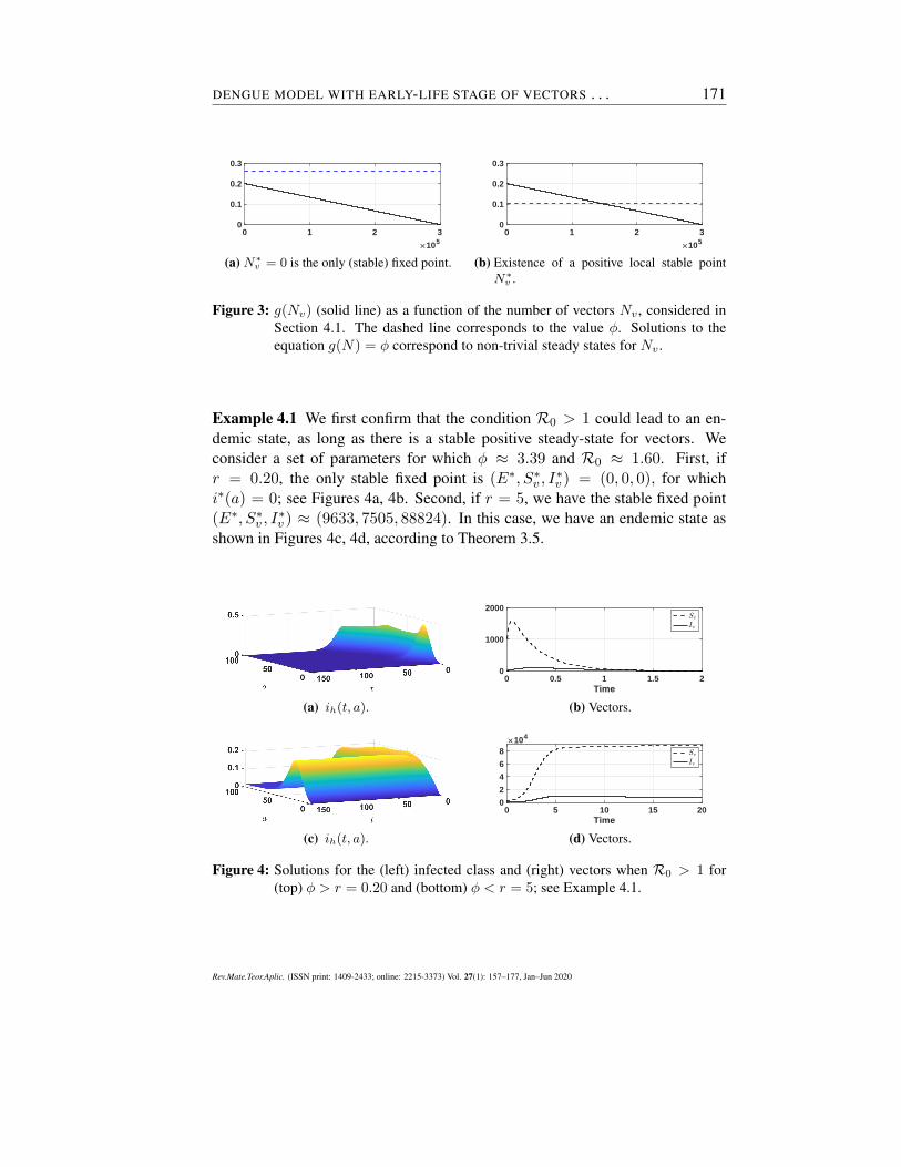
Figure 3: g(Nv) (solid line) as a function of the number of vectors Nv , considered inSection 4.1. The dashed line corresponds to the value ϕ. Solutions to theequation g(N) = ϕ correspond to non-trivial steady states for Nv .

Example 4.1 We first confirm that the condition R0 > 1 could lead to an en-demic state, as long as there is a stable positive steady-state for vectors. Weconsider a set of parameters for which ϕ ≈ 3.39 and R0 ≈ 1.60. First, ifr = 0.20, the only stable fixed point is (E∗, S∗

v , I∗v ) = (0, 0, 0), for which

i∗(a) = 0; see Figures 4a, 4b. Second, if r = 5, we have the stable fixed point(E∗, S∗

v , I∗v ) ≈ (9633, 7505, 88824). In this case, we have an endemic state as

shown in Figures 4c, 4d, according to Theorem 3.5.

(a) ih(t, a).

0 0.5 1 1.5 2Time

0

1000

2000

(b) Vectors.

(c) ih(t, a).

0 5 10 15 20Time

0

2

4

6

8104

(d) Vectors.

Figure 4: Solutions for the (left) infected class and (right) vectors when R0 > 1 for(top) ϕ > r = 0.20 and (bottom) ϕ < r = 5; see Example 4.1.



Example 4.2 In this example we confirm that the condition R0 < 1 is sufficientto guarantee a disease-free steady state. We take r = 5 and reduce β such thatR0 < 1. The infected class reaches a disease-free state as shown in Figure 5a,according to Theorem 3.4. Even though there exists a positive state for vectors(E∗, N∗

v ) as shown in Figure 5b, we observe that I∗v = 0.

(a) i(t, a).

0 5 10 15 20Time

0

5

10 104

(b) Vectors.

Figure 5: When R0 < 1, the disease-free state is stable, even though there is a positivesteady state for vectors (Rv > 1); see Example 4.2.

Example 4.3 We now consider the case R0 > 1 with initial conditions E0 = 0,Sv0 = 10, Iv0 = 1, ih(0, a) = rh(0, a) = 0 (no infected or immune humans attime t = 0); see results for the infected class in Figure 6. It is clear that R0 > 1guarantees an endemic state as long as vectors can survive.

(a) ih(t, a).

0 5 10 15 20Time

0

2

4

6

8104

(b) Vectors.

Figure 6: When R0 > 1, if there exists a positive state for vectors (Rv > 1) we canobserve an endemic state on humans; see Example 4.3.

4.2 Multiple vector demographic states

In a second set of experiments we use

g(Nv) = re−Nv/c1(sin(c2Nv) + 1), (12)

for given constants r, c1, c2. Here, r is the vector per-capita fertility rate,c1 is a form of vector control and c2 represents the variations in vectordensities; for a particular choice of parameters see Figure 1. Equation(12) represents the different growth rates of vectors for the wet and dryseasons. In this way, we simulate variations based on vector control efforts,obtaining multiple vector demographic steady states for (E∗, N∗

v ).



For the particular choice of parameters we have used, we obtain eight positivefixed points. Numerically we confirm that four of them are locally stable.

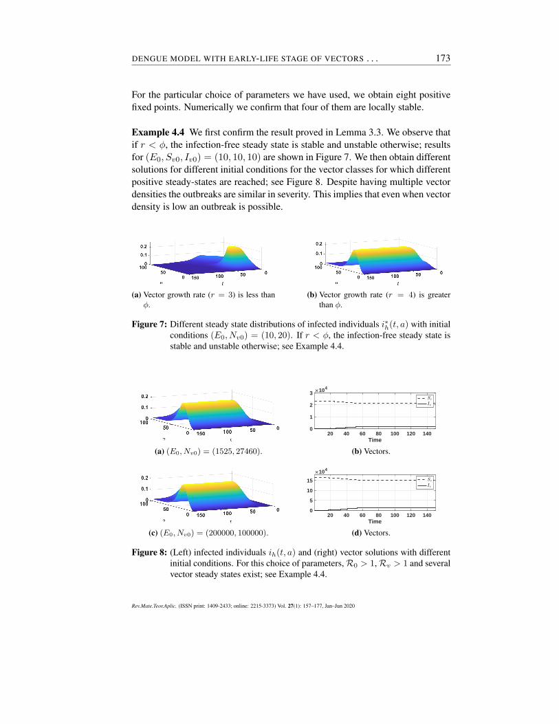
Example 4.4 We first confirm the result proved in Lemma 3.3. We observe thatif r < ϕ, the infection-free steady state is stable and unstable otherwise; resultsfor (E0, Sv0, Iv0) = (10, 10, 10) are shown in Figure 7. We then obtain differentsolutions for different initial conditions for the vector classes for which differentpositive steady-states are reached; see Figure 8. Despite having multiple vectordensities the outbreaks are similar in severity. This implies that even when vectordensity is low an outbreak is possible.

(a) Vector growth rate (r = 3) is less thanϕ.

(b) Vector growth rate (r = 4) is greaterthan ϕ.

Figure 7: Different steady state distributions of infected individuals i∗h(t, a) with initialconditions (E0, Nv0) = (10, 20). If r < ϕ, the infection-free steady state isstable and unstable otherwise; see Example 4.4.

(a) (E0, Nv0) = (1525, 27460).

20 40 60 80 100 120 140Time

0

1

2

3 104

(b) Vectors.

(c) (E0, Nv0) = (200000, 100000).

20 40 60 80 100 120 140Time

0

5

10

15

104

(d) Vectors.

Figure 8: (Left) infected individuals ih(t, a) and (right) vector solutions with differentinitial conditions. For this choice of parameters, R0 > 1, Rv > 1 and severalvector steady states exist; see Example 4.4.



Example 4.5 Similarly as Example 4.2, we confirm that R0 < 1 is sufficient forthe disease to die out, even in the presence of a positive population of vectors. Inthis case, (E∗, N∗

v ) = (7430, 74305), but I∗v = 0; see Figure 9. Even when thedemographic vector number is bigger than one the disease can be under controlwhen R0 < 1.

0 5 10 15 20Time

0

2

4

6

8104

Figure 9: R0 < 1 is sufficient to guarantee that (left) ih(a) = 0 and (right) I∗v = 0,even though S∗

v > 0, E∗ > 0; see Example 4.5.

Example 4.6 Similarly as Example 4.3, we confirm that R0 > 1 implies theexistence of an endemic state, as long as a positive equilibrium state exists forthe vectors to survive; see Figure 10.

0 5 10 15 20Time

0

1

2

3 104

Figure 10: (Left) ih(t, a) and (right) (E(t), Sv(t), Iv(t)) for R0 > 1; see Example 4.6.Initially all humans are susceptible and (E0, Sv0, Iv0) = (0, 10, 1).

4.3 Effect of seasonality on dengue dynamics

In most places where dengue is endemic, seasonal variations in vector pop-ulations play a major role in disease transmission. Moreover, it determinesthe distribution of resources allocated for preventive/control measures. Typi-cally, dengue incidence is correlated with the rainy season. The importanceof understanding seasonal variations per location could potentially help publichealth officials to allocate resources, as well as having better preventive/controlmeasures to reduce dengue incidence (focused primarily towards the reductionof vector breeding sites).



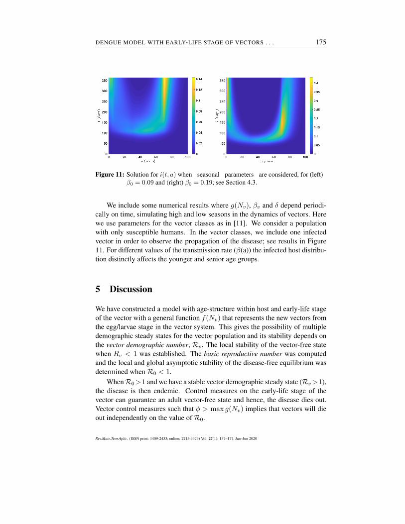
Figure 11: Solution for i(t, a) when seasonal parameters are considered, for (left)β0 = 0.09 and (right) β0 = 0.19; see Section 4.3.

We include some numerical results where g(Nv), βv and δ depend periodi-cally on time, simulating high and low seasons in the dynamics of vectors. Herewe use parameters for the vector classes as in [11]. We consider a populationwith only susceptible humans. In the vector classes, we include one infectedvector in order to observe the propagation of the disease; see results in Figure11. For different values of the transmission rate (β(a)) the infected host distribu-tion distinctly affects the younger and senior age groups.

5 Discussion

We have constructed a model with age-structure within host and early-life stageof the vector with a general function f(Nv) that represents the new vectors fromthe egg/larvae stage in the vector system. This gives the possibility of multipledemographic steady states for the vector population and its stability depends onthe vector demographic number, Rv. The local stability of the vector-free statewhen Rv < 1 was established. The basic reproductive number was computedand the local and global asymptotic stability of the disease-free equilibrium wasdetermined when R0 < 1.

When R0>1 and we have a stable vector demographic steady state (Rv>1),the disease is then endemic. Control measures on the early-life stage of thevector can guarantee an adult vector-free state and hence, the disease dies out.Vector control measures such that ϕ > max g(Nv) implies that vectors will dieout independently on the value of R0.



There are important public health implications when we are able to includehost age distribution, which can determine better strategies for hospitalized indi-viduals. Furthermore, control measures on the early-life stage of the vector caneffectively change the landscape on how public health officials lead preventionefforts before the onset of a dengue outbreak.

Acknowledgements

We thank the Research Center in Pure and Applied Mathematics and the Math-ematics Department at Universidad de Costa Rica for their support during thepreparation of this manuscript. The authors gratefully acknowledge institutionalsupport for project B8747 from an UCREA grant from the Vice Rectory forResearch at Universidad de Costa Rica.

References

[1] F. Brauer, C. Castillo-Chavez, A. Mubayi, S. Towers, Some models forepidemics of vector-transmitted diseases, Infect. Dis. Model. 1(2016), no.1, 79–87. doi: 10.1016/j.idm.2016.08.001

[2] Centers for Disease Control and Prevention, Dengue, https://www.cdc.gov/Dengue/

[3] L. Esteva, C. Vargas, Analysis of a dengue disease transmissionmodel, Math. Biosci. 150 (1998), no. 2, 131–151. doi: 10.1016/S0025-5564(98)10003-2

[4] L. Esteva, C. Vargas, A model for dengue disease with variable humanpopulation, J. Math. Biol. 38(1999), no. 3, 220–240. doi: 10.1007/s002850050147

[5] Z. Feng, J.X. Velasco-Hernández, Competitive exclusion in a vector-hostmodel for the dengue fever, J. Math. Biol. 35(1997), no. 5, 523–544. doi:10.1007/s002850050064

[6] D.J. Gubler, Resurgent vector-borne diseases as a global health prob-lem, Emerging Infect. Dis. 4(1998), no. 3, 442–450. doi: 10.3201/eid0403.980326

[7] E. Harris, E. Videa, L. Pérez, E. Sandoval, Y. Téllez, M.L. Pérez, R.Cuadra, J. Rocha, W. Idiaquez, R.E. Alonso, M.A. Delgado, L.A. Campo,



F. Acevedo, A. Gonzalez, J.J. Amador, A. Balmaseda, Clinical, epidemio-logic, and virologic features of dengue in the 1998 epidemic in Nicaragua,Am. J. Trop. Med. Hyg. 63(2000), no. 1-2, 5–11. doi: 10.4269/ajtmh.2000.63.5

[8] C.A. Manore, K.S. Hickmann, S. Xu, H.J. Wearing, J.M. Hyman, Compar-ing dengue and chikungunya emergence and endemic transmission in A.aegypti and A. albopictus, J. Theor. Biol. 356(2014), 174–191. doi: 10.1016/j.jtbi.2014.04.033

[9] D. Murillo, S. Holechek, A. Murillo, F. Sanchez, C. Castillo-Chavez, Verti-cal transmission in a two-strain model of dengue fever, Letters in Biomath-ematics 1(2014), no. 2, 249–271. doi: 10.1080/23737867.2014.11414484

[10] F. Sanchez, L. Barboza, D. Burton, A. Cintrón-Arias, Comparative anal-ysis of dengue versus chikungunya outbreaks in Costa Rica, JournalRicerche di Matematica 67(2018), no. 1, 163–174. doi: 10.1007/s11587-018-0362-3

[11] F. Sanchez, M. Engman, L. Harrington, C. Castillo-Chavez, Models fordengue transmission and control, in: A. Gumel, C. Castillo-Chavez, D.P.Clemence, & R.E. Mickens (Eds.) Mathematical studies on human dis-ease dynamics. Emerging paradigms and challenges (Snowbird, Utah,2005), Contemp. Math. 410(2006), 311–326. doi: 10.1090/conm/410/07734

[12] F. Sanchez, D. Murillo, C. Castillo-Chavez, Change in host behavior andits impact on the transmission dynamics of dengue, in: R.P. Mondani (Ed.)BIOMAT 2011, World Scientific, Singapore, 2012, pp. 191–203. doi: 10.1142/9789814397711_0013


Documents

DENGUE MODEL WITH EARLY LIFE STAGE OF VECTORS AND …