Demonstration of the Cascadia G-FASTGeodetic Earthquake Early Warning Systemfor the Nisqually, Washington, Earthquakeby Brendan W. Crowell, David A. Schmidt, Paul Bodin, John E. Vidale,Joan Gomberg, J. Renate Hartog, Victor C. Kress, Timothy I. Melbourne,Marcelo Santillan, Sarah E. Minson, and Dylan G. Jamison

ABSTRACT

A prototype earthquake early warning (EEW) system is cur-rently in development in the Pacific Northwest. We have takena two-stage approach to EEW: (1) detection and initial charac-terization using strong-motion data with the Earthquake AlarmSystems (ElarmS) seismic early warning package and (2) the trig-gering of geodetic modeling modules using Global NavigationSatellite Systems data that help provide robust estimates oflarge-magnitude earthquakes. In this article we demonstratethe performance of the latter, the Geodetic First Approximationof Size and Time (G-FAST) geodetic early warning system, usingsimulated displacements for the 2001 Mw 6.8 Nisqually earth-quake. We test the timing and performance of the two G-FASTsource characterization modules, peak ground displacement scal-ing, and Centroid MomentTensor-driven finite-fault-slip mod-eling under ideal, latent, noisy, and incomplete data conditions.We show good agreement between source parameters computedby G-FASTwith previously published and postprocessed seismicand geodetic results for all test cases and modeling modules, andwe discuss the challenges with integration into the U.S. Geologi-cal Survey’s ShakeAlert EEW system.

INTRODUCTION

Earthquake early warning (EEW) systems provide seconds to mi-nutes of advanced warning after rupture initiation and prior tothe arrival of strong ground shaking at a location. The method-ology currently employed uses seismic networks to quickly char-acterize the magnitude and epicenter from P waves at thestations nearest to the epicenter and sends an alert over a broadregion before the S wave arrives. A common problem with seis-mically derived magnitudes for EEW is the saturation of the sig-nal at large magnitudes (M >7; Brown et al., 2011). One causeof saturation is the limited P-wave time window available foranalysis before the arrival of the S wave at nearby stations, whichcan be shorter than the duration of the rupture source for largeevents. Another culprit in magnitude saturation is the high-passfiltering of strong-motion records, which is performed to min-

imize long-period drifts due to sensor rotations and tilts duringintegration to velocity and displacement (Melgar, Bock, et al.,2013). This filtering reduces the low-frequency content of theearthquake recording, which is critical to characterize largeearthquakes.

Geodetic observations provide an additional constraint thatdoes not saturate for large-magnitude events. Global PositioningSystem (GPS) displacement waveforms on their own have beenshown to be useful for near-real-time magnitude determinationusing peak ground displacement (PGD) scaling relationships(Crowell et al., 2013; Melgar et al., 2015), rapid CentroidMoment Tensor (CMT) determination for size and orientation(Melgar et al., 2012; Melgar, Crowell, et al., 2013; O'Toole et al.,2013), and finite-fault methods that use rapidly computed co-seismic offsets to compute slip on the fault (Crowell et al., 2009,2012; Allen and Ziv, 2011; Ohta et al., 2012; Wright et al.,2012; Böse et al., 2013; Colombelli et al., 2013; Minson et al.,2014; Grapenthin et al., 2014a). PGD scaling has been shown tobe slower than P-wave-based methods because (1) large earth-quakes take time to reach their peak amplitudes and (2) theS waves that determine PGD travel little more than half thespeed of P waves. In the case of a large offshore event like the2011 Mw 9.0 Tohoku-Oki earthquake, an initial PGD-basedmagnitude estimate of M 8.5 would be available 50 s followingnucleation, which still would have been useful for warning largepopulation centers like Tokyo (Melgar et al., 2015). Methodsthat rely on coseismic offsets can have an impact on traditionalEEW only in extreme cases (i.e., large earthquakes far from pop-ulation centers with S-wave travel times on the order of a fewminutes or preferential geometrical alignment of stations), buttheir major utility is in proper characterization of earthquakeimpact for tsunami early warning and hazard response (Blewittet al., 2006; Ohta et al., 2012). In addition, Crowell et al. (2013)have shown that when strong-motion accelerations and GPS dis-placements are combined using a multirate Kalman filter (Bocket al., 2011), the impact of magnitude saturation is greatly di-minished, even using only the first 5 s of data after the P-wavearrival. This method requires collocated GPS and strong-

930 Seismological Research Letters Volume 87, Number 4 July/August 2016 doi: 10.1785/0220150255

motion instruments, which is currently rare in western NorthAmerica.

The subduction environment of Cascadia motivates theneed for a joint seismic and geodetic EEW system to rapidlycharacterize all possible earthquakes within the region. Poten-tial events include large megathrust events and outer-riseevents anywhere from the Mendocino triple junction to Van-couver Island, shallow crustal earthquakes in the Seattle andPortland metropolitan areas, and deep events within the slab.At the University of Washington (UW), development of theGeodetic First Approximation of Size and Time (G-FAST)system has been a high priority for operational EEW in theCascadia region.

G-FASTcontinuously receives real-time processed GPS timeseries from the Pacific Northwest Geodetic Array (PANGA) andmaintains a local data buffer. G-FAST receives event triggersfrom a seismic detection module, such as Earthquake AlarmSystems (ElarmS), and starts with an estimate of the location,timing, and size of the earthquake. G-FAST first estimates mag-nitude and depth from PGD scaling. It then invokes a model-ing suite to estimate a CMT and finite-fault parameters.

To explore the performance of the system, we imple-mented a test system that reads in synthetic data and xml mes-sages from a seismic detection module and outputs theinformation in a simulated real-time mode, leaving theback-end modeling modules untouched. The simulated systemallows us to vary the latency, data completeness, and noise totest the robustness of magnitude, timing, and slip estimatesfrom G-FAST.

In this article, we first give an overview of G-FAST and thesynthetic test system. Then, we demonstrate the performanceduring a simulation of the 28 February 2001Mw 6.8 Nisquallyearthquake. The Nisqually earthquake was a deep intraslabevent located at the southern end of Puget Sound, roughly50 km deep, and caused damage costing several billion dollarsin the Seattle area (Ichinose et al., 2004). The Nisqually earth-quake is a good test case for G-FAST, because intraplate eventshave a higher probability of occurrence in the Pacific North-west than a megathrust event (∼30–50 year recurrence, withthe prior comparable 1949 Olympia and 1965 Seattle–Tacomaevents, Ichinose et al., 2004), and it caused shaking over a wideregion (modified Mercalli intensity [MMI] VI–VII through-out the Puget Lowlands, see Data and Resources), and was re-corded with fairly low signal-to-noise surface displacements.The components of G-FAST have been independently testedand validated on much larger earthquakes elsewhere in Japan,Chile, Indonesia, and southern California (Crowell et al.,2012, 2013; Melgar et al., 2012, 2015); so the motivation fortesting G-FAST on the Nisqually earthquake is to determinethe performance and resolution toward the lower end of de-tectability and to ascertain statistics on the range of possiblesolutions by varying the latency, noise, and data completeness.Finally, we discuss how to best improve the EEWsystem basedon the simulation results and challenges associated with inte-gration into the ShakeAlert system, which is the EEW system

currently under development by the U.S. Geological Survey(USGS) with university partners (Given et al., 2014).

JOINT EARTHQUAKE EARLY WARNING SYSTEM

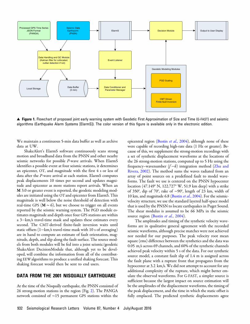
The current ShakeAlert system uses three different seismic al-gorithms for estimating location, magnitude, and origin time(OT): ElarmS (Kuyuk et al., 2014), Virtual Seismologist (VS,Cua and Heaton, 2007), and OnSite (Böse et al., 2009). TheCalifornia system runs all three algorithms, whereas the PacificNorthwest system currently only uses ElarmS. Several GPS-based algorithms that utilize rapidly computed coseismic offsetsare currently under development, including G-larmS (Grape-nthin et al., 2014a) and BEFORES (Minson et al., 2014). Inthis article, we document an additional geodetic module underdevelopment, G-FAST. What distinguishes the G-FAST ap-proach is its combination of different types of analyses. It firstestimates source depth and magnitude from PGD. This is sim-ilar to GPSlip (Böse et al., 2013), which also determines sourcestrength from PGD, but with the addition of solving for sourcedepth as well, giving G-FAST an advantage in subduction zoneenvironments where earthquakes occur over a wide range ofdepths. G-FAST then uses a geodetically derived focal mecha-nism to determine the fault orientation, builds a discretizedfault plane with that orientation, and then inverts for the staticslip distribution on that fault plane. This final slip model is ascomplex as the BEFORES geodetic EEW algorithm (Minsonet al., 2014), which rapidly updates both the fault orientationand the spatial distribution of accumulated slip on that faultplane as the rupture evolves, and is more complex than the G-larmS geodetic EEW source model (Grapenthin et al., 2014a),which only allows for along-strike variations in slip amplitude.Thus, the G-FAST slip model is probably better suited than G-larmS to subduction zone earthquakes that can have significantalong-dip variation in slip. The G-FAST approach is also sub-stantially faster than G-larmS because we can obtain the PGD-determined magnitude and source depth before the wavefieldhas converged to the static state, and it is probably comparablein speed to BEFORES, although direct head-to-head perfor-mance testing between the various geodetic EEW algorithmshas yet to be done. The flowchart of operations of G-FAST isshown in Figure 1. The system consists of two independentpackages: (1) a data aggregator and buffer that runs continu-ously and (2) a triggered modeling suite that activates uponreceiving an alert from the seismic warning system (currentlyElarmS). High-rate real-time GPS positions are continuouslyreceived at the Pacific Northwest Seismic Network (PNSN)from PANGA through the JSON protocol (see Data andResources). The PANGA solutions are integer ambiguity-resolved precise point positions (Zumberge et al., 1997) esti-mated at 1 s epochs within the ITRF2008 reference frame (Al-tamimi et al., 2012) using satellite orbit and clock correctionsprovided by the International Global Navigation Satellite Sys-tems Service. Station positions are estimated independentlyand do not depend on a fixed reference station or network.

Seismological Research Letters Volume 87, Number 4 July/August 2016 931

We maintain a continuous 5-min data buffer as well as archivedata at UW.

ShakeAlert’s ElarmS software continuously scans strongmotion and broadband data from the PNSN and other nearbyseismic networks for possible P-wave arrivals. When ElarmSidentifies a possible event at four seismic stations, it determinesan epicenter, OT, and magnitude with the first 4 s or less ofdata after the P-wave arrival at each station. ElarmS computespeak displacements 10 times per second and updates magni-tude and epicenter as more stations report arrivals. When anM 3.0 or greater event is reported, the geodetic modeling mod-ules are initiated using the OTand epicenter from ElarmS. Thismagnitude is well below the noise threshold of detection withreal-time GPS (M ∼ 6), but we choose to trigger on all eventsreported by the seismic warning system. The PGD module es-timates magnitude and depth once four GPS stations are withina 3�km=s travel-time mask and updates these estimates everysecond. The CMT-derived finite-fault inversion waits untilstatic offsets (1�km=s travel-time mask with 10 s of averaging)are in hand to compute an estimate of fault orientation, mag-nitude, depth, and slip along the fault surface. The source mod-els from both modules will be fed into a joint seismic/geodeticShakeAlert DecisionModule that, although yet to be devel-oped, will combine the information from all of the contribut-ing EEWalgorithms to produce a unified shaking forecast. Thisshaking forecast would then be sent to end users.

DATA FROM THE 2001 NISQUALLY EARTHQUAKE

At the time of the Nisqually earthquake, the PNSN consisted of26 strong-motion stations in the region (Fig. 2). The PANGAnetwork consisted of ∼15 permanent GPS stations within the

epicentral region (Bustin et al., 2004), although none of thesewere capable of recording high-rate data (1 Hz or greater). Be-cause of this, we supplement the strong-motion recordings witha set of synthetic displacement waveforms at the locations ofthe 26 strong-motion stations, computed up to 5 Hz using thefrequency–wavenumber (f �k) integration method (Zhu andRivera, 2002). The method sums the waves radiated from anarray of point sources on a predefined fault to model wave-forms. The fault we use is centered on the PNSN hypocenterlocation (47.149° N, 122.727° W, 51.9 km deep) with a strikeof 350°, dip of 70°, rake of −90°, length of 23 km, width of10 km, and magnitude 6.8 (Bustin et al., 2004). For the seismic-velocity structure, we use the standard layered half-space modelthat is used by the PNSN to locate earthquakes in Puget Sound.The shear modulus is assumed to be 66 MPa in the seismicsource region (Bustin et al., 2004).

The amplitudes and timing of the synthetic velocity wave-forms are in qualitative general agreement with the recordedseismic waveforms, although precise matches were not achievednor needed for our purposes. The peak velocity root meansquare (rms) difference between the synthetics and the data was0:05 m=s across 69 channels, and 60% of the synthetic channelsachieved peak velocity within 5 s of the data. For our syntheticsource model, a constant fault slip of 1.4 m is assigned acrossthe fault plane with a rupture front that propagates from thehypocenter at 3:2 km=s. We did not attempt to account for anyadditional complexity of the rupture, which might better em-ulate the observed waveforms. For G-FAST, a simpler source issufficient because the largest impact on source estimation willbe the amplitudes of the displacement waveforms, the timing ofthe peak displacement, and the time in which the static offset isfully emplaced. The predicted synthetic displacements agree

▴ Figure 1. Flowchart of proposed joint early warning system with Geodetic First Approximation of Size and Time (G-FAST) and seismicalgorithms (Earthquake Alarm Systems [ElarmS]). The color version of this figure is available only in the electronic edition.

932 Seismological Research Letters Volume 87, Number 4 July/August 2016

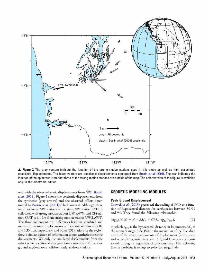
well with the observed static displacements from GPS (Bustinet al., 2004). Figure 2 shows the coseismic displacements fromthe synthetics (gray arrows) and the observed offsets deter-mined by Bustin et al. (2004) (black arrows). Although therewere not many GPS stations at the time, GPS station SATS iscollocated with strong-motion station UW.RWW, and GPS sta-tion SEAT is 6.1 km from strong-motion station UW.LAWT.The three-component rms differences between simulated andmeasured coseismic displacements at these two stations are 2.82and 1.35 mm, respectively, and other GPS stations in the regionshow a similar pattern of deformation to our synthetic coseismicdisplacements. We only use simulated displacements from thesubset of 26 operational strong-motion stations in 2001 becauseground motions were validated only at those stations.

GEODETIC MODELING MODULES

Peak Ground DisplacementCrowell et al. (2013) presented the scaling of PGD as a func-tion of hypocentral distance for earthquakes between M 5.4and 9.0. They found the following relationship:

EQ-TARGET;temp:intralink-;df1;323;166 log10�PGD� � A� BMw � CMw log10�rhyp�; �1�in which rhyp is the hypocentral distance in kilometers, Mw isthe moment magnitude, PGD is the maximum of the Euclidiannorm of the three components of displacement (north, east,and vertical) in centimeters, and A, B, and C are the constantssolved through a regression of previous data. The followinginverse problem is set up to solve for magnitude:

124˚W

0 50

km

123˚W 122˚W 121˚W

46˚N

47˚N

48˚N

1 cm

gray − FK coseismic

black − Bustin et al. [2004] coseismic

SEATUW.LAWT

UW.RWW/SATS

▴ Figure 2. The gray vectors indicate the location of the strong-motion stations used in this study as well as their associatedcoseismic displacements. The black vectors are coseismic displacements computed from Bustin et al. (2004). The star indicates thelocation of the epicenter. Note that three of the strong-motion stations are outside of the map. The color version of this figure is availableonly in the electronic edition.

Seismological Research Letters Volume 87, Number 4 July/August 2016 933

EQ-TARGET;temp:intralink-;df2;40;505GMw � b; �2�

EQ-TARGET;temp:intralink-;df3;40;488G �B� C log10�rhyp;1�

..

.

B� C log10�rhyp;n�

264

375; b �

log10�PGD1� − A...

log10�PGDn� − A

264

375:

�3�For G-FAST, we make a few key operational changes fromCrowell et al. (2013). First, we introduce a travel-time maskof 3 km=s given the earthquake OTs from ElarmS that ignoresall stations outside of the travel-time mask at a given time. Sec-ond, no magnitudes are estimated for fewer than four stations.Third, we utilize exponential distance weighting of the form:

EQ-TARGET;temp:intralink-;df4;40;335wi � exp�−

r2epi;i8r2epi;min

�; �4�

in which repi;i is the epicentral distance in kilometers of the ithstation and repi;min is the epicentral distance of the closest sta-tion. The distance weighting in equation (4) is a function ofthe epicentral distance, so as not to bias the depth grid searchdiscussed later toward shallower solutions. The factor of 8 inthe denominator is arbitrarily chosen through trial and error togive relatively high weight to many close stations before drop-ping off exponentially. The magnitude is then found by solving

EQ-TARGET;temp:intralink-;df5;40;191WGMw � Wb; �5�in whichW is a diagonal matrix of station weights wi. We recali-brate the regression constants of Crowell et al. (2013) with theinclusion of the distance weight matrix using data for theTohoku-Oki, Tokachi-Oki, and El Mayor–Cucapah earth-quakes. We find A � −6:687, B � 1:500, and C � −0:214,with an improved magnitude uncertainty of 0.17 magnitudeunits. These coefficients are different from an analysis byMelgar

et al. (2015) using an expanded data set of 10 earthquakes re-corded by GPS alone. The recalibration of the Crowell et al.(2013) regression uses only seismogeodetic (collocated GPS andstrong-motion stations) data and hence represents a minimalnoise solution. However, in general, all the regression solutionspredict similar magnitudes within the bounds of uncertainty ofthe method (�0:3 magnitude units).

Finally, we introduce a grid search for the earthquakedepth. ElarmS assumes a depth of 8 km for all events, becausethat is the average seismogenic depth in California. But thePGD algorithm requires proper depth characterization, giventhat the depth affects the PGD pattern. It is also importantto discriminate between shallow crustal earthquakes and deeperevents that are located along the plate interface or within theslab. The grid-search method simply computes the magnitudeat 1 km intervals between 0 and 100 km depth and chooses thedepth that maximizes the variance reduction (VR) defined by

EQ-TARGET;temp:intralink-;df6;311;301VR ��1 −

jjb − GMwjjjjbjj

�× 100: �6�

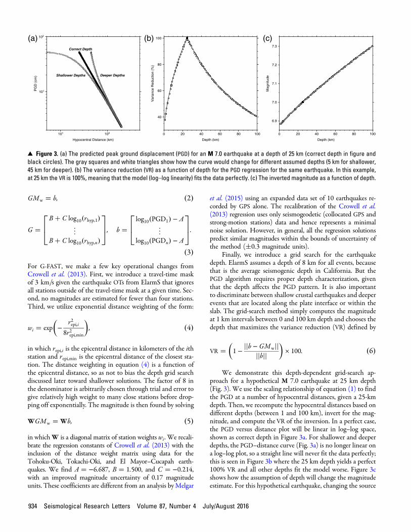
We demonstrate this depth-dependent grid-search ap-proach for a hypothetical M 7.0 earthquake at 25 km depth(Fig. 3). We use the scaling relationship of equation (1) to findthe PGD at a number of hypocentral distances, given a 25-kmdepth. Then, we recompute the hypocentral distances based ondifferent depths (between 1 and 100 km), invert for the mag-nitude, and compute the VR of the inversion. In a perfect case,the PGD versus distance plot will be linear in log–log space,shown as correct depth in Figure 3a. For shallower and deeperdepths, the PGD–distance curve (Fig. 3a) is no longer linear ona log–log plot, so a straight line will never fit the data perfectly;this is seen in Figure 3b where the 25 km depth yields a perfect100% VR and all other depths fit the model worse. Figure 3cshows how the assumption of depth will change the magnitudeestimate. For this hypothetical earthquake, changing the source

101

10(a) (b) (c)2P

GD

(cm

)

101 102

Hypocentral Distance (km)

Shallower Depths Deeper Depths

Correct Depth

40

60

80

100

Var

ianc

e R

educ

tion

(%)

0 20 40 60 80 100

Depth (km)

6.9

7.0

7.1

7.2

7.3

Mag

nitu

de

0 20 40 60 80 100

Depth (km)

▴ Figure 3. (a) The predicted peak ground displacement (PGD) for an M 7.0 earthquake at a depth of 25 km (correct depth in figure andblack circles). The gray squares and white triangles show how the curve would change for different assumed depths (5 km for shallower,45 km for deeper). (b) The variance reduction (VR) as a function of depth for the PGD regression for the same earthquake. In this example,at 25 km the VR is 100%, meaning that the model (log–log linearity) fits the data perfectly. (c) The inverted magnitude as a function of depth.

934 Seismological Research Letters Volume 87, Number 4 July/August 2016

depth for 1–100 km will change the magnitude by 0.4 mag-nitude units. Although this magnitude change is not large, theprediction of the strength of expected ground shaking is sen-sitive to different source depths.

CMT-Driven Slip Modeling on a Finite FaultComputing the CMT is important, because it allows us to de-termine the fault orientation and location as well as magnitude,which have important implications for expected ground mo-tions and tsunami potential. Melgar et al. (2012) showed howto compute the CMT using rapidly computed static offsets in alayered half-space. For efficiency and simplicity, we chose tosolve the problem in a homogeneous half-space using the staticdisplacement field analytical solution for the moment tensorfrom Hashima et al. (2008) and the references therein. The gen-eral solution for the displacement field ui�x� for a given momenttensor Mpq at a point x from a source at point ξ is given by

EQ-TARGET;temp:intralink-;df7;52;541ui�x� �1

8πμR2 �γ�3ζiζpζq − ζiδpq − ζpδqi − ζqδip�

� 2ζqδipMpq; �7�in which i, p, and q are the three Cartesian directions,γ � �3K � μ�=�3K � 4μ�, μ and K are the rigidity and bulkmodulus, respectively, δip is the Kronecker delta, R is the source–receiver distance defined by

EQ-TARGET;temp:intralink-;df8;52;434R ���������������������������������������������������������������������������x1 − ξ1�2 � �x2 − ξ2�2 � �x3 − ξ3�2

q; �8�

and the scaled source–receiver distance is

EQ-TARGET;temp:intralink-;df9;52;379ζi �xi − ξiR

: �9�

The following inverse problem for n stations is set up and solvedwith linear least squares

EQ-TARGET;temp:intralink-;df10;52;311

u1;1u2;1u3;1

..

.

u1;nu2;nu3;n

26666666666664

37777777777775

�

G111;1 G121;1 G131;1 G221;1 G231;1 G331;1

G112;1 G122;1 G132;1 G222;1 G232;1 G332;1

G113;1 G123;1 G133;1 G223;1 G233;1 G333;1

..

. ... ..

. ... ..

. ...

G111;n G121;n G131;n G221;n G231;n G331;n

G112;n G122;n G132;n G222;n G232;n G332;n

G113;n G123;n G133;n G223;n G233;n G333;n

26666666666664

37777777777775

×

M11

M12

M13

M22

M23

M33

2666666664

3777777775; �10�

with the Green’s functions,Gipq;n, being defined by equation (7).The displacements ui;n are the static offsets on each of the threedirectional components, which are computed by taking the aver-age of the first 10 s of data that arrive after a travel-time mask of1 km=s is used. Note, displacements are with respect to the sta-tion position at the OT of the earthquake. This travel-time maskis overly conservative, but we want to minimize inclusion of anydynamic motions that may contaminate the static offset measure-ments and do not want to rely on some other metric to deter-mine if the solution is stable. The displacements and Green’sfunctions are both rotated into the radial, transverse, and verticaldirections, and the moment tensor is decomposed into the mainand auxiliary fault planes using the Python ObsPy package (seeData and Resources). Rather than performing a grid search forthe centroid location, we use the epicentral location from ElarmSand only perform a grid search for the depth using the same VRmaximization scheme as was done for PGD.

A slip inversion on a finite fault provides a more accuratecharacterization of the event when compared to a point source,especially given a potential large megathrust event in Cascadia.Melgar, Crowell, et al. (2013) outlined the difficulties of usinga simple point-source approximation for computing the CMTfrom static offsets for theTohoku-Oki earthquake. In that case,they found using a fixed hypocenter point source would lead toan accurate moment tensor solution; however, the model fitwould be poor (VR < 50%) and could not be trusted in realtime. A slip inversion on a finite fault does not have these issuesif the fault plane is large enough, is in the correct region, andhas reasonable strike and dip angles. Grapenthin et al. (2014a)investigated the slip inversion sensitivity to location and faultorientation errors. Although a general rule-of-thumb is diffi-cult here, because this is highly dependent on the earthquakesource and network geometry, they found that variations in lo-cation, dip, and strike become less important for deeper events,and for shallower events the orientations should be within 5°.Misplacement of the center of the fault can impact the magni-tude error by up to 0.5 magnitude units within 20 km.

For G-FAST’s slip inversion, we use the method of Crowellet al. (2012) where the fault geometry is defined by the CMT,and the Green’s functions are prescribed by Okada’s formu-lation (Okada, 1985) in a homogeneous half-space. The centerof the fault plane is defined by the ElarmS epicenter and thedepth computed from the CMT. The along-strike and along-dip dimensions of the fault are defined by scaling relationshipsfrom Dreger and Kaverina (2000), based on the CMTmagni-tude. We are not concerned that the CMTmagnitude may bean overestimate, because this will only make the potential slipsurface larger; the inversion does not prescribe slip in areas if thedata misfit does not call for it. The CMT-computed depth alsowill not greatly impact the result, because it defines the center ofthe fault and the along-dip dimension will cover the majority ofthe possible seismogenic zone. Of the two fault planes from theCMT, we pick the one that minimizes the misfit as the finalsolution. Laplacian regularization with a generalized smoothingparameter described in Crowell et al. (2012) is used. The staticoffsets used are the same as for the CMT inversion.

Seismological Research Letters Volume 87, Number 4 July/August 2016 935

SIMULATIONS

We first run G-FAST assuming no data latency and no datanoise to find the ideal source characterization and timing withthe synthetic displacements. The ElarmS location, timing, andmagnitude are found using the actual strong-motion data be-cause the short-term average/long-term average algorithm fordetecting P-wave arrivals requires some level of noise to operateefficiently.

To obtain realistic operational system performance, werun four simulations and for each conduct 1000 trials of G-FAST. The four simulations test the impacts of (1) randomlygenerated latencies, (2) high-rate GPS station noise, (3) datadropouts, and (4) latency + noise + dropouts. We performthese simulations to test the stability and robustness of thesource solutions, obtain realistic timing and to see how eachfactor impacts the results for future improvements. We gener-ate integer latencies from a Poisson distribution with a mean of6 s. Data latency from the PANGA/Plate Boundary Observa-tory (PBO) network is generally much better than this and isimproving (phase and range distribution <1 s, processing anddistribution <3 s); however, we choose a conservative estimate.

We generate the station noise using the power spectrumfor 40-km relative GPS positions from Genrich and Bock(2006), a combination of white (f 0), flicker (1=f ), and ran-dom-walk (1=f 2) noise. We choose to simulate noise insteadof superimposing recorded noise time series from PANGA tohave control over the range of potential noise sources. Wecompared the power spectra of the 10 most complete timeseries recorded at the PNSN in real time from PANGA on15 September 2015 with the power spectra of Genrich andBock (2006). At periods less than 10 s, the PANGA real-timesolutions matched perfectly with the Genrich and Bock (2006)power spectra. At periods between 5 min and 10 s, the real-timepower spectra are systematically lower than the simulation powerspectra we use, indicating that the simulations in this article re-present a worst-case scenario, especially at long periods.

The real-time data completeness rate for PBO in theCascadia region is generally better than 95% (D. Mencin,personal comm., 2015, UNAVCO). Most data dropouts aredue to a few stations with less than ideal telemetry, but for thesake of argument, we assume a data return rate of 85% for allstations during our simulations. For a large earthquake, we areuncertain as to the telemetry robustness, and therefore we wantto consider a worst-case scenario. For these simulations, wesimply remove 15% of the data points at random each trial.We do not consider spatial or temporal correlation of dropoutseven though a significant percentage of dropouts will be dueto the temporary failure of a single telemetry path that mayhandle several stations. Even without explicitly consideringspatially correlated dropouts, removing 15% of the data (whendata completeness is generally much better than 95%) fromeach station at random will explore the range of possible sol-utions, and the source parameters should be robustly estimatedwith 1000 trials.

RESULTS

Peak Ground DisplacementThe evolution of PGD magnitude and depth estimates overtime is shown in Figure 4 for the ideal case as well as the foursimulations for the Nisqually earthquake. In the ideal case, thefirst magnitude estimates from PGD are available 17 s after theOT, trailing ElarmS by about 4 s. The initial PGD magnitudeestimate isM 6.47 (at 17 s) andM 6.43 for ElarmS (at 12.8 s).The arrival of strong shaking in Seattle, 60 km northwest of theepicenter, is at 23 s after OT, so ElarmS would provide a 10 swarning to Seattle and an updated warning from PGD is avail-able 6 s prior to strong shaking. For both ElarmS and PGD, themagnitude estimates start out small and increase quickly overthe first ∼10 s to their final stable magnitude estimate. In theideal case, no PGD estimate is provided to locations within51 km of the epicenter. The magnitude estimates over timedo not vary much for the ideal case; the full range of magnitudeestimates is 0.2 magnitude units. The stable magnitude esti-mate (>30 s) from PGD (M 6:7� 0:3) and from ElarmS(M 6.9) are both close to the true magnitude of 6.8.

The depth estimate in the ideal case starts out shallow butquickly converges to the final solution of 52 km, exactly theinput model depth (51.9 km) and close to the Global CMTsolution of 46.8 km. ElarmS assumes a depth of 8 km becauseit was designed to represent the average seismogenic depth inCalifornia; this has an impact on the prediction of travel timesof strong shaking as well as estimating ground motions inShakeAlert. Assuming a 1=r attenuation, the 8 km depth at anepicentral distance of 20 km would overestimate strong shak-ing by a factor of 2.5 versus the 50 km depth given the samemagnitude earthquake. The assumption of a shallower depthwould lead to a smaller PGD magnitude estimate, however, asdemonstrated by Figure 3c. We plan on modifying ElarmS inthe Pacific Northwest to accommodate a depth grid search,however, dealing with other aspects of tuning ElarmS for theregion has taken precedence (Hartog et al., 2016; see Data andResources).

All four simulations produce stable estimates of magnitudeafter about 30 s, although the range of magnitude estimatesprior to 30 s is less than a magnitude unit, and the range ofsolutions quickly narrows to ∼0:3 magnitude units. Evidenceof this tight distribution of magnitude estimates is shown inFigure 5, which contains histograms of the simulations at30 s after OT. The impact of latency is minimal on the stabilityof magnitude, and its impact is concentrated toward the begin-ning of the earthquake, although latency is the only parameterthat impacts the warning time. The average first-alert time inthe latency simulations is 21.9 s after OT, which matches the5 s Poissonian distributed latency used in the simulations. Byabout 70 s after OT, the latency simulations are exactly thesame as the ideal case. This is not surprising, because latencywill only alter the order in which data come in and are utilized;after some time, all the important data (i.e., the recording ofpeak ground motions) will be available. Latency does, however,

936 Seismological Research Letters Volume 87, Number 4 July/August 2016

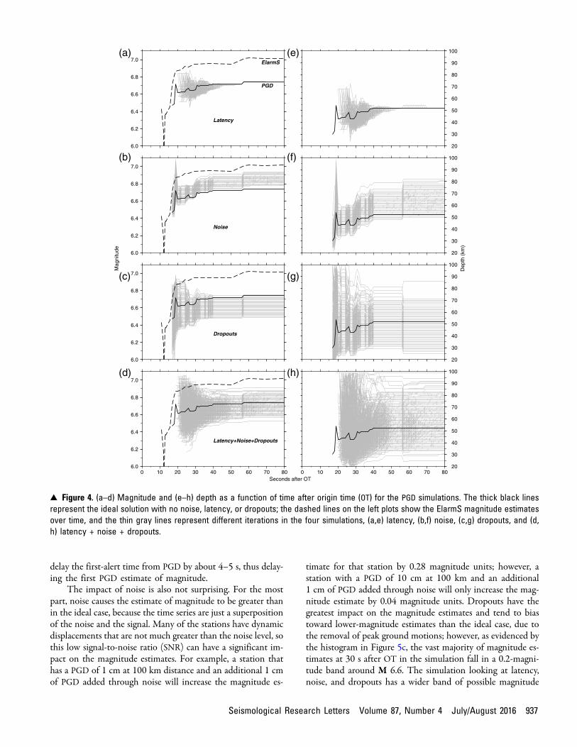
delay the first-alert time from PGD by about 4–5 s, thus delay-ing the first PGD estimate of magnitude.

The impact of noise is also not surprising. For the mostpart, noise causes the estimate of magnitude to be greater thanin the ideal case, because the time series are just a superpositionof the noise and the signal. Many of the stations have dynamicdisplacements that are not much greater than the noise level, sothis low signal-to-noise ratio (SNR) can have a significant im-pact on the magnitude estimates. For example, a station thathas a PGD of 1 cm at 100 km distance and an additional 1 cmof PGD added through noise will increase the magnitude es-

timate for that station by 0.28 magnitude units; however, astation with a PGD of 10 cm at 100 km and an additional1 cm of PGD added through noise will only increase the mag-nitude estimate by 0.04 magnitude units. Dropouts have thegreatest impact on the magnitude estimates and tend to biastoward lower-magnitude estimates than the ideal case, due tothe removal of peak ground motions; however, as evidenced bythe histogram in Figure 5c, the vast majority of magnitude es-timates at 30 s after OT in the simulation fall in a 0.2-magni-tude band around M 6.6. The simulation looking at latency,noise, and dropouts has a wider band of possible magnitude

6.0

6.2

6.4

6.6

6.8

7.0(a)

(b)

(c)

(d)

(e)

(f)

(g)

(h)

ElarmS

PGD

Latency

6.0

6.2

6.4

6.6

6.8

7.0

Mag

nitu

de

Noise

6.0

6.2

6.4

6.6

6.8

7.0

Dropouts

6.0

6.2

6.4

6.6

6.8

7.0

0 10 20 30 40 50 60 70 80Seconds after OT

Latency+Noise+Dropouts

20

30

40

50

60

70

80

90

100

20

30

40

50

60

70

80

90

100

Dep

th (

km)

20

30

40

50

60

70

80

90

100

20

30

40

50

60

70

80

90

100

0 10 20 30 40 50 60 70 80

▴ Figure 4. (a–d) Magnitude and (e–h) depth as a function of time after origin time (OT) for the PGD simulations. The thick black linesrepresent the ideal solution with no noise, latency, or dropouts; the dashed lines on the left plots show the ElarmS magnitude estimatesover time, and the thin gray lines represent different iterations in the four simulations, (a,e) latency, (b,f) noise, (c,g) dropouts, and (d,h) latency + noise + dropouts.

Seismological Research Letters Volume 87, Number 4 July/August 2016 937

estimates of about 0.3 magnitude units (Fig. 4d), but the resultis still robust and only slightly larger than the previously pub-lished uncertainties of the PGD method (Crowell et al., 2013;Melgar et al., 2015).

The depth results have a much greater range of possiblesolutions, but like the magnitude estimates, the histogramsin Figure 5 show the distributions are much tighter than theyappear in Figure 4. Latency, once again, shows that it has thesmallest impact on the results and eventually converges to theideal solution by 70 s. The noise simulations bias the depthestimates toward deeper depths, although all the simulations at

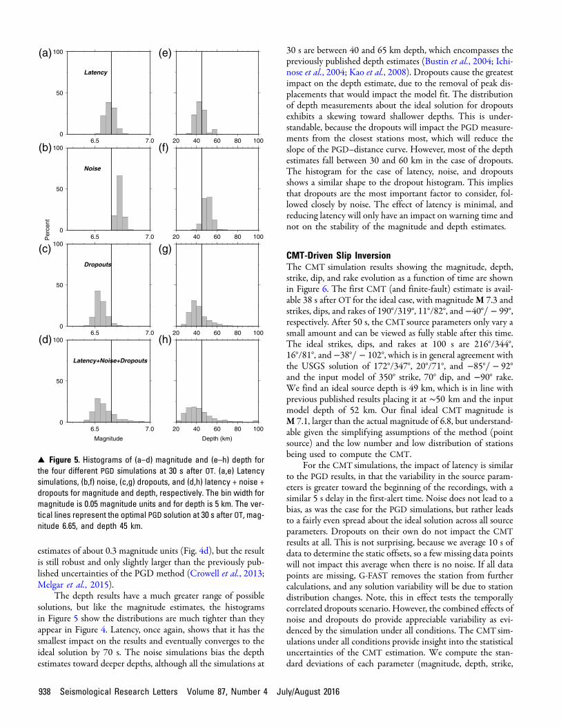
30 s are between 40 and 65 km depth, which encompasses thepreviously published depth estimates (Bustin et al., 2004; Ichi-nose et al., 2004; Kao et al., 2008). Dropouts cause the greatestimpact on the depth estimate, due to the removal of peak dis-placements that would impact the model fit. The distributionof depth measurements about the ideal solution for dropoutsexhibits a skewing toward shallower depths. This is under-standable, because the dropouts will impact the PGD measure-ments from the closest stations most, which will reduce theslope of the PGD–distance curve. However, most of the depthestimates fall between 30 and 60 km in the case of dropouts.The histogram for the case of latency, noise, and dropoutsshows a similar shape to the dropout histogram. This impliesthat dropouts are the most important factor to consider, fol-lowed closely by noise. The effect of latency is minimal, andreducing latency will only have an impact on warning time andnot on the stability of the magnitude and depth estimates.

CMT-Driven Slip InversionThe CMT simulation results showing the magnitude, depth,strike, dip, and rake evolution as a function of time are shownin Figure 6. The first CMT (and finite-fault) estimate is avail-able 38 s after OT for the ideal case, with magnitudeM 7.3 andstrikes, dips, and rakes of 190°/319°, 11°/82°, and −40°= − 99°,respectively. After 50 s, the CMTsource parameters only vary asmall amount and can be viewed as fully stable after this time.The ideal strikes, dips, and rakes at 100 s are 216°/344°,16°/81°, and −38°= − 102°, which is in general agreement withthe USGS solution of 172°/347°, 20°/71°, and −85°= − 92°and the input model of 350° strike, 70° dip, and −90° rake.We find an ideal source depth is 49 km, which is in line withprevious published results placing it at ∼50 km and the inputmodel depth of 52 km. Our final ideal CMT magnitude isM 7.1, larger than the actual magnitude of 6.8, but understand-able given the simplifying assumptions of the method (pointsource) and the low number and low distribution of stationsbeing used to compute the CMT.

For the CMT simulations, the impact of latency is similarto the PGD results, in that the variability in the source param-eters is greater toward the beginning of the recordings, with asimilar 5 s delay in the first-alert time. Noise does not lead to abias, as was the case for the PGD simulations, but rather leadsto a fairly even spread about the ideal solution across all sourceparameters. Dropouts on their own do not impact the CMTresults at all. This is not surprising, because we average 10 s ofdata to determine the static offsets, so a few missing data pointswill not impact this average when there is no noise. If all datapoints are missing, G-FAST removes the station from furthercalculations, and any solution variability will be due to stationdistribution changes. Note, this in effect tests the temporallycorrelated dropouts scenario. However, the combined effects ofnoise and dropouts do provide appreciable variability as evi-denced by the simulation under all conditions. The CMT sim-ulations under all conditions provide insight into the statisticaluncertainties of the CMT estimation. We compute the stan-dard deviations of each parameter (magnitude, depth, strike,

0

50

100(a)

(b)

(c)

(d)

(e)

(f)

(g)

(h)

6.5 7.0

Latency

0

50

100

Per

cent

6.5 7.0

Noise

0

50

100

6.5 7.0

Dropouts

0

50

100

6.5 7.0

Magnitude

Latency+Noise+Dropouts

20 40 60 80 100

20 40 60 80 100

20 40 60 80 100

20 40 60 80 100

Depth (km)

▴ Figure 5. Histograms of (a–d) magnitude and (e–h) depth forthe four different PGD simulations at 30 s after OT. (a,e) Latencysimulations, (b,f) noise, (c,g) dropouts, and (d,h) latency + noise +dropouts for magnitude and depth, respectively. The bin width formagnitude is 0.05 magnitude units and for depth is 5 km. The ver-tical lines represent the optimal PGD solution at 30 s after OT, mag-nitude 6.65, and depth 45 km.

938 Seismological Research Letters Volume 87, Number 4 July/August 2016

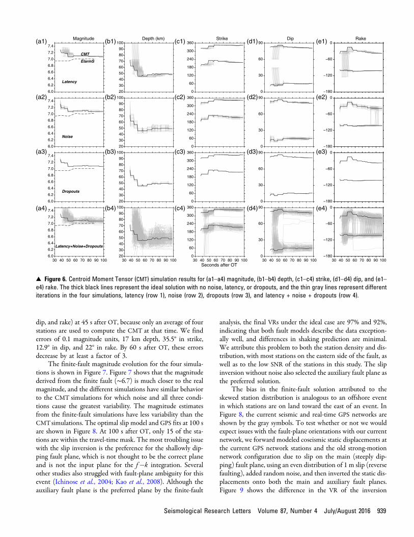
dip, and rake) at 45 s after OT, because only an average of fourstations are used to compute the CMT at that time. We finderrors of 0.1 magnitude units, 17 km depth, 35.5° in strike,12.9° in dip, and 22° in rake. By 60 s after OT, these errorsdecrease by at least a factor of 3.

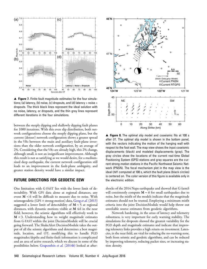
The finite-fault magnitude evolution for the four simula-tions is shown in Figure 7. Figure 7 shows that the magnitudederived from the finite fault (∼6:7) is much closer to the realmagnitude, and the different simulations have similar behaviorto the CMT simulations for which noise and all three condi-tions cause the greatest variability. The magnitude estimatesfrom the finite-fault simulations have less variability than theCMTsimulations. The optimal slip model and GPS fits at 100 sare shown in Figure 8. At 100 s after OT, only 15 of the sta-tions are within the travel-time mask. The most troubling issuewith the slip inversion is the preference for the shallowly dip-ping fault plane, which is not thought to be the correct planeand is not the input plane for the f �k integration. Severalother studies also struggled with fault-plane ambiguity for thisevent (Ichinose et al., 2004; Kao et al., 2008). Although theauxiliary fault plane is the preferred plane by the finite-fault

analysis, the final VRs under the ideal case are 97% and 92%,indicating that both fault models describe the data exception-ally well, and differences in shaking prediction are minimal.We attribute this problem to both the station density and dis-tribution, with most stations on the eastern side of the fault, aswell as to the low SNR of the stations in this study. The slipinversion without noise also selected the auxiliary fault plane asthe preferred solution.

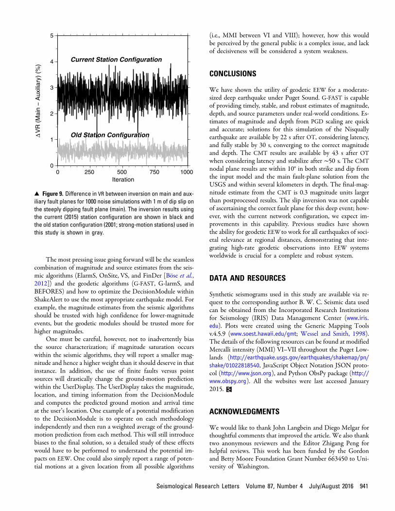
The bias in the finite-fault solution attributed to theskewed station distribution is analogous to an offshore eventin which stations are on land toward the east of an event. InFigure 8, the current seismic and real-time GPS networks areshown by the gray symbols. To test whether or not we wouldexpect issues with the fault-plane orientations with our currentnetwork, we forward modeled coseismic static displacements atthe current GPS network stations and the old strong-motionnetwork configuration due to slip on the main (steeply dip-ping) fault plane, using an even distribution of 1 m slip (reversefaulting), added random noise, and then inverted the static dis-placements onto both the main and auxiliary fault planes.Figure 9 shows the difference in the VR of the inversion

6.0

6.2

6.4

6.6

6.8

7.0

7.2

7.4(a1)

(a2)

(a3)

(a4)

(b1)

(b2)

(b3)

(b4)

(c1)

(c2)

(c3)

(c4)

(d1)

(d2)

(d3)

(d4)

(e1)

(e2)

(e3)

(e4)

Magnitude

ElarmS

CMT

Latency

6.0

6.2

6.4

6.6

6.8

7.0

7.2

7.4

Noise

6.0

6.2

6.4

6.6

6.8

7.0

7.2

7.4

Dropouts

6.0

6.2

6.4

6.6

6.8

7.0

7.2

7.4

30 40 50 60 70 80 90 100

Latency+Noise+Dropouts

20

30

40

50

60

70

80

90

100Depth (km)

20

30

40

50

60

70

80

90

100

20

30

40

50

60

70

80

90

100

20

30

40

50

60

70

80

90

100

30 40 50 60 70 80 90 100

0

60

120

180

240

300

360Strike

0

60

120

180

240

300

360

0

60

120

180

240

300

360

0

60

120

180

240

300

360

30 40 50 60 70 80 90 100Seconds after OT

0

30

60

90Dip

0

30

60

90

0

30

60

90

0

30

60

90

30 40 50 60 70 80 90 100

−180

−120

−60

0Rake

−180

−120

−60

0

−180

−120

−60

0

30 40 50 60 70 80 90 100−180

−120

−60

0

▴ Figure 6. Centroid Moment Tensor (CMT) simulation results for (a1–a4) magnitude, (b1–b4) depth, (c1–c4) strike, (d1–d4) dip, and (e1–e4) rake. The thick black lines represent the ideal solution with no noise, latency, or dropouts, and the thin gray lines represent differentiterations in the four simulations, latency (row 1), noise (row 2), dropouts (row 3), and latency + noise + dropouts (row 4).

Seismological Research Letters Volume 87, Number 4 July/August 2016 939

between the steeply dipping and shallowly dipping fault planesfor 1000 iterations. With this even slip distribution, both net-work configurations choose the steeply dipping plane, but thecurrent (denser) network configuration shows a greater spreadin the VRs between the main and auxiliary fault-plane inver-sions than the older network configuration, by an average of2%. Considering that the VRs are already high, this 2% change,although small, is not an insignificant improvement. Althoughthis result is not as satisfying as we would desire, for a medium-sized deep earthquake, the current network configuration stillleads to an improvement in the fault-plane ambiguity, andgreater station density would have a similar impact.

FUTURE DIRECTIONS FOR GEODETIC EEW

One limitation with G-FAST lies with the lower limit of de-tectability. With GPS data alone at regional distances, anyevent M <6 will be difficult to measure due to noise. Withseismogeodetic (GPS + strong-motion) data, Geng et al. (2013)suggested a lower limit of detectability of M ∼ 5 at regionaldistances, with dynamic motions visible at M 4.6 in the nearfield; however, the seismic algorithms will effectively work toM <3. Understanding how to weight magnitude estimatesfrom G-FAST within the joint DecisionModule will be crucialgoing forward. The ShakeAlert DecisionModule takes the out-put of all the seismic algorithms and determines a best magni-tude, location, and OT; modifying this to handle PGDmagnitudes/depths and finite-fault information is complicatedand an area of active research, which we discuss in some of thepossibilities below. Grapenthin et al. (2014b) looked at after-

shocks of the 2014 Napa earthquake and showed that G-larmSwill consistently compute M ∼ 6 for small earthquakes due tonoise, but the misfit of the models indicate that the magnitudeestimates should not be trusted. Employing a minimum misfitcriteria into the joint DecisionModule would help throw outunreliable source estimates from geodetic algorithms.

Network hardening, in the areas of latency and telemetryrobustness, is very important for early warning stability. Thesimulations for dropouts showed the greatest variability for thePGD depth and magnitude estimates and indicate that improv-ing telemetry links provides a high return on investment. Laten-cies, in the near field, are vital for reducing the no-warning-zone,both from seismic and geodetic algorithms, and can be reducedby improving telemetry, reducing packet sizes, or increasing sta-tion density.

6.5

6.6

6.7

6.8

6.9

7.0(a)

(b)

(c)

(d)Mag

nitu

de

40 50 60 70 80 90 100

Latency

6.5

6.6

6.7

6.8

6.9

7.0

40 50 60 70 80 90 100Seconds after OT

Noise

40 50 60 70 80 90 100

Dropouts

40 50 60 70 80 90 100

Latency + Noise + Dropouts

▴ Figure 7. Finite-fault magnitude estimates for the four simula-tions; (a) latency, (b) noise, (c) dropouts, and (d) latency + noise +dropouts. The thick black lines represent the ideal solution withno noise, latency, or dropouts, and the thin gray lines representdifferent iterations in the four simulations.

124˚W 122˚W46˚N

48˚N

0 50

km

124˚W 123˚W 122˚W 121˚W46˚N

47˚N

48˚N

1 cm(black−Data;gray−Model)

Current PNSNCurrent RTGPS

45

50Dep

th (

km)

0 10 20 30 40 50 60Along Strike (km)

NE SW

1 m

▴ Figure 8. The optimal slip model and coseismic fits at 100 safter OT. The optimal slip model is shown in the bottom panel,with the vectors indicating the motion of the hanging wall withrespect to the foot wall. The map view shows the input coseismicdisplacements (black) and modeled displacements (gray). Thegray circles show the locations of the current real-time GlobalPositioning System (GPS) stations and gray squares are the cur-rent strong-motion stations in the Pacific Northwest Seismic Net-work (PNSN). The focal mechanism plot in the map view is theideal CMT computed at 100 s, which the fault plane (black circles)is centered on. The color version of this figure is available only inthe electronic edition.

940 Seismological Research Letters Volume 87, Number 4 July/August 2016

The most pressing issue going forward will be the seamlesscombination of magnitude and source estimates from the seis-mic algorithms (ElarmS, OnSite, VS, and FinDer [Böse et al.,2012]) and the geodetic algorithms (G-FAST, G-larmS, andBEFORES) and how to optimize the DecisionModule withinShakeAlert to use the most appropriate earthquake model. Forexample, the magnitude estimates from the seismic algorithmsshould be trusted with high confidence for lower-magnitudeevents, but the geodetic modules should be trusted more forhigher magnitudes.

One must be careful, however, not to inadvertently biasthe source characterization; if magnitude saturation occurswithin the seismic algorithms, they will report a smaller mag-nitude and hence a higher weight than it should deserve in thatinstance. In addition, the use of finite faults versus pointsources will drastically change the ground-motion predictionwithin the UserDisplay. The UserDisplay takes the magnitude,location, and timing information from the DecisionModuleand computes the predicted ground motion and arrival timeat the user’s location. One example of a potential modificationto the DecisionModule is to operate on each methodologyindependently and then run a weighted average of the ground-motion prediction from each method. This will still introducebiases to the final solution, so a detailed study of these effectswould have to be performed to understand the potential im-pacts on EEW. One could also simply report a range of poten-tial motions at a given location from all possible algorithms

(i.e., MMI between VI and VIII); however, how this wouldbe perceived by the general public is a complex issue, and lackof decisiveness will be considered a system weakness.

CONCLUSIONS

We have shown the utility of geodetic EEW for a moderate-sized deep earthquake under Puget Sound. G-FAST is capableof providing timely, stable, and robust estimates of magnitude,depth, and source parameters under real-world conditions. Es-timates of magnitude and depth from PGD scaling are quickand accurate; solutions for this simulation of the Nisquallyearthquake are available by 22 s after OT, considering latency,and fully stable by 30 s, converging to the correct magnitudeand depth. The CMT results are available by 43 s after OTwhen considering latency and stabilize after ∼50 s. The CMTnodal plane results are within 10° in both strike and dip fromthe input model and the main fault-plane solution from theUSGS and within several kilometers in depth. The final-mag-nitude estimate from the CMT is 0.3 magnitude units largerthan postprocessed results. The slip inversion was not capableof ascertaining the correct fault plane for this deep event; how-ever, with the current network configuration, we expect im-provements in this capability. Previous studies have shownthe ability for geodetic EEWto work for all earthquakes of soci-etal relevance at regional distances, demonstrating that inte-grating high-rate geodetic observations into EEW systemsworldwide is crucial for a complete and robust system.

DATA AND RESOURCES

Synthetic seismograms used in this study are available via re-quest to the corresponding author B. W. C. Seismic data usedcan be obtained from the Incorporated Research Institutionsfor Seismology (IRIS) Data Management Center (www.iris.edu). Plots were created using the Generic Mapping Toolsv.4.5.9 (www.soest.hawaii.edu/gmt; Wessel and Smith, 1998).The details of the following resources can be found at modifiedMercalli intensity (MMI) VI–VII throughout the Puget Low-lands (http://earthquake.usgs.gov/earthquakes/shakemap/pn/shake/01022818540, JavaScript Object Notation JSON proto-col (http://www.json.org), and Python ObsPy package (http://www.obspy.org). All the websites were last accessed January2015.

ACKNOWLEDGMENTS

We would like to thank John Langbein and Diego Melgar forthoughtful comments that improved the article. We also thanktwo anonymous reviewers and the Editor Zhigang Peng forhelpful reviews. This work has been funded by the Gordonand Betty Moore Foundation Grant Number 663450 to Uni-versity of Washington.

0

1

2

3

4

5Δ

VR

(M

ain

− A

uxili

ary)

(%

)

0 250 500 750 1000Iteration

Current Station Configuration

Old Station Configuration

▴ Figure 9. Difference in VR between inversion on main and aux-iliary fault planes for 1000 noise simulations with 1 m of dip slip onthe steeply dipping fault plane (main). The inversion results usingthe current (2015) station configuration are shown in black andthe old station configuration (2001; strong-motion stations) used inthis study is shown in gray.

Seismological Research Letters Volume 87, Number 4 July/August 2016 941

REFERENCES

Allen, R. M., and A. Ziv (2011). Application of real-time GPS to earth-quake early warning, Geophys. Res. Lett. 38, L16310, doi: 10.1029/2011GL047947.

Altamimi, Z., L. Métivier, and X. Collilieux (2012). ITRF2008 plate mo-tion model, J. Geophys. Res. 117, no. B07402, doi: 10.1029/2011JB008930.

Blewitt, G., C. Kreemer, W. C. Hammond, H.-P. Plag, S. Stein, and E.Okal (2006). Rapid determination of earthquake magnitude usingGPS for tsunami warning systems, Geophys. Res. Lett. 33, L11309,doi: 10.1029/2006GL026145.

Bock, Y., D. Melgar, and B. W. Crowell (2011). Real-time strong-motionbroadband displacements from collocated GPS and accelerometers,Bull. Seismol. Soc. Am. 101, no. 6, 2904–2925, doi: 10.1785/0120110007.

Böse, M., E. Hauksson, K. Solanki, H. Kanamori, Y.-M. Wu, and T. H.Heaton (2009). A new trigger criterion for improved real-timeperformance of onsite earthquake early warning in southern Cal-ifornia, Bull. Seismol. Soc. Am. 99, no. 2A, 897–905, doi: 10.1785/0120080034.

Böse, M., T. H. Heaton, and E. Hauksson (2012). Real-time finitefault rupture detector (FinDer) for large earthquakes, Geophys. J.Int. 191, no. 2, 803–812, doi: 10.1111/j.1365-246X.2012.05657.x.

Böse, M., T. Heaton, and K. Hudnut (2013). Combining real-timeseismic and GPS data for earthquake early warning (invited),American Geophysical Union, Fall Meeting 2013, abstract numberG51B-05.

Brown, H. M., R. M. Allen, M. Hellweg, O. Khainovski, D. Neuhauser,and A. Souf (2011). Development of the ElarmS methodology forearthquake early warning: Realtime application in California andoffline testing in Japan, Soil Dyn. Earthq. Eng. 31, no. 2, 188–200, doi: 10.1016/j.soildyn.2010.03.008.

Bustin, A., R. D. Hyndman, A. Lambert, J. Ristau, J. He, H. Dragert, andM. Van der Kooij (2004). Fault parameters of the Nisqually earth-quake determined from moment tensor solutions and the surfacedeformation from GPS and InSAR, Bull. Seismol. Soc. Am. 94,no. 2, 363–376, doi: 10.1785/0120030073.

Colombelli, S., R. M. Allen, and A. Zollo (2013). Application of real-timeGPS to earthquake early warning in subduction and strike-slip envi-ronments, J. Geophys. Res. 118, no. 7, 3448–3461, doi: 10.1002/jgrb.50242.

Crowell, B. W., Y. Bock, and D. Melgar (2012). Real-time inversion ofGPS data for finite fault modeling and rapid hazard assessment,Geophys. Res. Lett. 39, L09305, doi: 10.1029/2012GL051318.

Crowell, B. W., Y. Bock, and M. Squibb (2009). Demonstration of earth-quake early warning using total displacement waveforms from realtime GPS networks, Seismol. Res. Lett. 80, no. 5, 772–782, doi:10.1785/gssrl.80.5.772.

Crowell, B. W., D. Melgar, Y. Bock, J. S. Haase, and J. Geng (2013).Earthquake magnitude scaling using seismogeodetic data,Geophys. Res. Lett. 40, no. 23, 6089–6094, doi: 10.1002/2013GL058391.

Cua, G., and T. Heaton (2007). The virtual seismologist (VS) method:A Bayesian approach to earthquake early warning, in EarthquakeEarly Warning Systems, P. Gasparini, G. Manfredi, and J. Zschau(Editors), Springer, Berlin, Germany, 97–130, doi: 10.1007/978-3-540-72241-0_7.

Dreger, D., and A. Kaverina (2000). Seismic remote sensing for the earth-quake source process and near-source strong shaking: A case studyof the October 16, 1999 Hector Mine earthquake, Geophys. Res.Lett. 27, no. 13, 1941–1944.

Geng, J., Y. Bock, D. Melgar, B. W. Crowell, and J. S. Haase (2013). Anew seismogeodetic approach applied to GPS and accelerometerobservations of the 2012 Brawley seismic swarm: Implications forearthquake early warning, Geochem. Geophys. Geosyst. 14, no. 7,2124–2142, doi: 10.1002/ggge.20144.

Genrich, J. F., and Y. Bock (2006). Instantaneous geodetic positioningwith 10–50 Hz GPS measurements: Noise characteristics andimplications for monitoring networks, J. Geophys. Res. 111,no. B03403, doi: 10.1029/2005JB003617.

Given, D. D., E. S. Cochran, T. Heaton, E. Hauksson, R. Allen, P.Hellweg, J. Vidale, and P. Bodin (2014). Technical implementationplan for the ShakeAlert production system: An earthquake earlywarning system for the west coast of the United States, U.S. Geol.Surv. Open-File Rept. 2014-1097, 25 pp., doi: 10.3133/ofr20141097.

Grapenthin, R., I. A. Johanson, and R. M. Allen (2014a). Operationalreal-time GPS-enhanced earthquake early warning, J. Geophys. Res.119, no. 10, 7944–7965, doi: 10.1002/2014JB011400.

Grapenthin, R., I. Johanson, and R. M. Allen (2014b). The 2014Mw 6.0Napa earthquake, California: Observations from real-time GPS-en-hanced earthquake early warning, Geophys. Res. Lett. 41, no. 23,8269–8276, doi: 10.1002/2014GL061923.

Hartog, J. R., V. C. Kress, S. D. Malone, P. Bodin, J. E. Vidale, and B. W.Crowell (2016). Earthquake early warning: ShakeAlert in thePacific Northwest, Bull. Seismol. Soc. Am. (accepted).

Hashima, A., Y. Takada, Y. Fukahata, and M. Matsu’ura (2008). Generalexpressions for internal deformation due to a moment tensor in anelastic/viscoelastic multilayered half-space, Geophys. J. Int. 175,no. 3, 992–1012, doi: 10.1111/j.1365-246X.2008.03837.x.

Ichinose, G. A., H. K. Thio, and P. G. Somerville (2004). Rupture processand near-source shaking of the 1965 Seattle–Tacoma and 2001Nisqually, intraslab earthquakes, Geophys. Res. Lett. 31, L10604,doi: 10.1029/2004GL019668.

Kao, H., K. Wang, R.-Y. Chen, I. Wada, J. He, and S. D. Malone (2008).Identifying the rupture plane of the 2001 Nisqually, Washington,earthquake, Bull. Seismol. Soc. Am. 98, no. 3, 1546–1558, doi:10.1785/0120070160.

Kuyuk, H. S., R. M. Allen, H. Brown, M. Hellweg, I. Henson, and D.Neuhauser (2014). Designing a network-based earthquake earlywarning algorithm for California: ElarmS-2, Bull. Seismol. Soc.Am. 104, no. 1, 162–173, doi: 10.1785/0120130146.

Melgar, D., Y. Bock, and B. W. Crowell (2012). Real-time centroidmoment tensor determination for large earthquakes from local andregional displacement records, Geophys. J. Int. 188, no. 2, 703–718,doi: 10.1111/j.1365-246X.2011.05297.x.

Melgar, D., Y. Bock, D. Sanchez, and B. W. Crowell (2013). On robustand reliable automated baseline corrections for strong motion seismol-ogy, J. Geophys. Res. 118, no. 3, 1177–1187, doi: 10.1002/jgrb.50135.

Melgar, D., B. W. Crowell, Y. Bock, and J. S. Haase (2013). Rapid mod-eling of the 2011Mw 9.0 Tohoku-Oki earthquake with seismogeod-esy, Geophys. Res. Lett. 40, no. 12, 2963–2968, doi: 10.1002/grl.50590.

Melgar, D., B. W. Crowell, J. Geng, R. M. Allen, Y. Bock, S. Riquelme, E.Hill, M. Protti, and A. Ganas (2015). Earthquake magnitude calcu-lations without saturation from the scaling of peak ground displace-ment, Geophys. Res. Lett. 42, no. 13, 5197–5205, doi: 10.1002/2015GL064278.

Minson, S. E., J. R. Murray, J. O. Langbein, and J. S. Gomberg (2014).Real-time inversions for finite fault slip models and rupture geom-etry based on high-rate GPS data, J. Geophys. Res. 119, no. 4, 3201–3231, doi: 10.1002/2013JB010622.

Ohta, Y., T. Kobayashi, H. Tsushima, S. Miura, R. Hino, T. Takasu, H.Fujimoto, T. Iinuma, K. Tachibana, T. Demachi, et al. (2012).Quasi real-time fault model estimation for near-field tsunami fore-casting based on RTK-GPS analysis: Application to the 2011 To-hoku-Oki earthquake (Mw 9.0), J. Geophys. Res. 117, no. B02311,doi: 10.1029/2011JB008750.

Okada, Y. (1985). Surface deformation to shear and tensile faults in ahalf-space, Bull. Seismol. Soc. Am. 75, 1135–1154.

O'Toole, T. B., A. P. Valentine, and J. H. Woodhouse (2013). Earthquakesource parameters from GPS-measured static displacements withpotential for real-time application, Geophys. Res. Lett. 40, no. 1,60–65, doi: 10.1029/2012GL054209.

942 Seismological Research Letters Volume 87, Number 4 July/August 2016

Wessel, P., and W. H. F. Smith (1998). New, improved version of genericmapping tools released, Eos Trans. AGU 79, no. 47, 579, doi:10.1029/98EO00426.

Wright, T. J., N. Houlié, M. Hildyard, and T. Iwabuchi (2012). Real-time, reliable magnitudes for large earthquakes from 1 Hz GPS pre-cise point positioning: The 2011 Tohoku-Oki (Japan) earthquake,Geophys. Res. Lett. 39, L12302, doi: 10.1029/2012GL051894.

Zhu, L., and L. A. Rivera (2002). A note on the dynamic and static displace-ments from a point source in multi-layered media,Geophys. J. Int. 148,no. 3, 619–627, doi: 10.1046/j.1365-246X.2002.01610.x.

Zumberge, J. F., M. B. Heflin, D. C. Jefferson, M. M. Watkins, and F. H.Webb (1997). Precise point positioning for the efficient and robustanalysis of GPS data from large networks, J. Geophys. Res. 102,no. B3, 5005–5017, doi: 10.1029/96JB03860.

Brendan W. CrowellDavid A. Schmidt

Paul BodinJohn E. Vidale

J. Renate HartogVictor C. Kress

Department of Earth and Space SciencesUniversity of Washington

Johnson Hall Room-070, Box 3513104000 15th Avenue NE

Seattle, Washington 98195-1310 U.S.A.crowellb@uw.edu

Joan GombergU.S. Geological Survey

Earthquake Science CenterUniversity of Washington

Johnson Hall Room-070, Box 3513104000 15th Avenue NE

Seattle, Washington 98195-1310 U.S.A.

Timothy I. MelbourneMarcelo Santillan

Department of Geological SciencesCentral Washington University

400 E. University Way, MS 7418Ellensburg, Washington 98926 U.S.A.

Sarah E. MinsonU.S. Geological Survey

Earthquake Science Center345 Middlefield Road, MS 977

Menlo Park, California 94025-3591 U.S.A.

Dylan G. JamisonDepartment of Earth and Environmental Sciences

University of Waterloo200 University Avenue West

Waterloo, OntarioCanada N2L 3G1

Published Online 8 June 2016

Seismological Research Letters Volume 87, Number 4 July/August 2016 943