DEMANDFUNCTIONSWITHINFERIOR GOODS: THE IMPLICIT

DEMAND FUNCTIONS WITH INFERIOR GOODS: THE IMPLICIT

FUNCTION APPROACH

SHUJI TAKAHASHI

Institute of Economics and Business Administration, Kanto Gakuin University

Yokohama, Kanagawa 236-8501 Japan

[email protected]

Received December 2018; Accepted February 2019

Abstract

In this article, we propose a numerically computable utility function that can apply to

inferior goods. The implicit function and its optimization technique are fully used. Since the

implicit function is carefully formulated, it works well as a standard utility function. This

technique ensures tractability and extendability. We propose the following: (1) a simple utility

function of an inferior good which contains only two parameters; (2) a total cost function and

its extension to the Cobb-Douglas production function with an inferior input; (3) a generalized

utility function whose Engel-curve always stems from the origin.

Keywords: inferior goods, utility function, production function, implicit function

JEL Classification Codes: D01, D11, D21

I. Introduction

Inferior goods are widely observed in an economy. It is natural for consumers to upgrade

or downgrade their purchases according to their budget. However, a numerically computable

utility function for inferior goods has not been fully developed yet and has been studied by

researchers. Epstein and Spiegel (2000) found a simple production function for an inferior

input, which has only two parameters in the minimum setting, although it does not explain why

the input is inferior or how to extend their two-variable model to n-variables. Moffatt (2002)

uses a hyperbola to avoid intersection of the indifference curves and succeeds in dealing with

Giffen goods. Doi, Iwasa, and Shinomura (2006) use the logarithmic function in their

formulation.

In this study, we propose the implicit function approach to deal with inferior goods.1The

utility function, u(x, y), is given by U(u, x, y)=0, which is unsolvable for u . At first glance,

this function appears awkward and difficult to use or incompatible with the economic theory.

Hitotsubashi Journal of Economics 60 (2019), pp.79-105. Ⓒ Hitotsubashi University

1 We focus on the two-goods case in this study. However, this two-goods model is extended to the n-goods case. The

n-goods case will be presented in another paper.

However, we find that our implicit utility function gives all types of tractable functions such as

the compensated demand, normal demand, and total cost functions. These are compatible with

the economic theory.

The remainder of the paper consists of three parts. First, Sections 2 and 3 illustrate the

structure of our implicit function using the simplest model, which contains only two

parameters, a and c. Second, Section 4 discusses the production function which contains full

parameters.2

Furthermore, we show the addition of an inferior good to the Cobb-Douglas

production function. Third, the generalized utility function is presented in Section 5, where both

goods are normal when income is low; however, either can change from a normal to an inferior

good as income increases.

II. Illustration

Let us denote utility by u, and the quantities of the two goods by x and y. If the utility

function is

u(x, y)=xa+y, (0<a<1),

then x would never be an inferior good. For x to be an inferior good, its marginal utility must

gradually reduce with an increase in overall utility u, since x is less favored by high-utility

individuals. Therefore, we place a decreasing function,1

uc , (c>0) before xa, and reformulate

u=xa+y into

u=1

ucxa+y. (1)

Thus, u(x, y) is given by the implicit function,

U(u, x, y)≡1

ucxa+y−u=0.

One of the solvable cases for u is when c=1. When c=1, (1) is given by

u=1

uxa+y,

which gives u2−uy−xa=0. Therefore, this can be solved as

u(x, y)=y+ y2+4xa

2. (2)

Equation (2) resembles the quadratic formula in mathematics.3If we solve the problem of

minimizing the expenditure px+y, where p denotes the relative price, subject to

HITOTSUBASHI JOURNAL OF ECONOMICS [June80

2 Sections 4 and 5 are independent of the earlier sections. The reader can begin to read from Section 4 or 5.3 The production function of Epstein and Spiegel (2000) resembles (2). It can be expressed as u=(y+x)

−βx,

(0<α<1, β<1 and ν>0).

u0−(y+ y2+4xa )/2=0 for a fixed u0, then we get x(p, u0)=(a/(u0p))1

1a as the compensated

demand function, which is decreasing in u. Thus, we can confirm that (2) is the utility function

of an inferior good.

We must note that although (1) is unsolvable for u in general, it can give the utility level.

This is explained as follows. Let us decompose (1) into two functions: LHS(u)=u and

RHS(u)=ucxa+y . The former is the 45-degree line in Figure 1. The latter is the downward

sloping curve. These always intersect, in this case at point A, where LHS(u)=RHS(u) . Then,

(1) always gives u as a real and unique number.

Let us consider the case where c=1. The indifference curves of u=u1xa+y are illustrated

in Figure 2(i). The indifference curves for u=1 and u=2 are given by

1=xa+y, and

2=(1/2)xa+y,

respectively, where the latter equation has the larger constant term and smaller coefficient of x

than the former. Therefore, the two indifference curves never intersect for non-negative x and y.

The simplest case is that of perfect substitutes (a=1),

u=u1x+y.

The indifference curves for u=1, 2, 3,..., are given by 1=x+y, 2=(1/2)x+y, 3=(1/3)x+y,...,

respectively. These equations are illustrated in Figure 2 (ii). The gradient of the indifferencecurves decreases with an increase in u.

DEMAND FUNCTIONS WITH INFERIOR GOODS: THE IMPLICIT FUNCTION APPROACH2019] 81

u

y

LHS

RHS LHS

RHS

A

s

The LHS curve is on the left-hand side of u=ucxa+y and the RHS curve on the right-hand side. They always

have a single intersection point, point A. The projection of point A on the x-axis represents the real value s that we use

as the utility level. An increase in x or y shifts the RHS curve upward. Therefore, marginal utility is always positive.

FIGURE 1. UTILITY LEVEL

III. Consumer’s Demand Function with Inferior Goods

Let m=px+y be the budget constraint, where m is an income level, and p is the relative

price. For a given m, the problem faced by a consumer is

max x, y u

s.t ucxa+y−u=0, and m−px−y=0.

To solve this problem, we use the Lagrange function4

L=u+μ(ucxa+y−u)+λ(m−px−y) .

From this, we obtain

Lx=μaucxa1−λp=0 (3)

Ly=μ−λ=0 (4)

Lu=1+μ(−cuc1xa)=0

L=m−px−y=0 (5)

L =ucxa+y−u=0. (6)


4 An alternative method for solving this problem is available in Appendix A. In Appendix A, we use the optimization

technique for an implicit function to derive (7) and (12).

2

yy

3

u=2

(1/2)xa

u=1

1

2

1

u=4

u=3

u=2

u=1

xa

x1 4 9 x

(i): The indifference curve (IC) of u = 1 on (x, y) is given by 1=xa+y. If u increases to u = 2, the IC of u = 2

becomes 2=(1/2)xa+y. Therefore, the two ICs never intersect each other. This IC of u = 1 is represented by the xa

curve, being given by y=1−xa. The IC of u = 2 is represented by (1/2)xa. (ii): In the perfect substitute case, the

ICs are straight lines.

(i) Substitutes Case (ii) Perfect Substitutes Case

FIGURE 2. INDIFFERENCE CURVES

From (3) and (4) we obtain “the law of weighted equi-marginal utility” (aucxa1)/p=1,

from which we can also derive the compensated demands, x(p, u) and y(p, u) . Then, prior to

deriving the normal demand, x(p, m) and y(p, m), we derive x(p, u) and y(p, u).

From (3) and (4), we obtain

x(p, u)=a

ucp

1

1a

. (7)


y(p, u)=u−1

uc

a

ucp

a

1a

for u≥a

p a

1ac

, (8)

y(p, u)=0 for u≤a

p a

1ac

. (9)


x(p, u)=u1c

a for u≤a

p a

1ac

. (10)

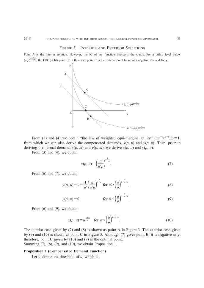
The interior case given by (7) and (8) is shown as point A in Figure 3. The exterior case given

by (9) and (10) is shown as point C in Figure 3. Although (7) gives point B, it is negative in y,

therefore, point C given by (10) and (9) is the optimal point.

Summing (7), (8), (9), and (10), we obtain Proposition 1.

Proposition 1 (Compensated Demand Function)

Let u denote the threshold of u, which is


u ≥ (a/p)1－a＋ca

u < (a/p)1－a＋ca

O x

y

A

B

C

a

b

Point A is the interior solution. However, the IC of our function intersects the x-axis. For a utility level below

(a/p)a

1ac, the FOC yields point B. In this case, point C is the optimal point to avoid a negative demand for y.

FIGURE 3. INTERIOR AND EXTERIOR SOLUTIONS

u(p)≡a

p a

1ac

.

(i) For u≥u, the compensated demands are

x(p, u)=a

ucp 1

1a

,

y(p, u)=u−1

uc a

ucp a

1a

.

where the utility and price elasticity of x(p, u) are constant

∂x

∂u

u

x=

−c

1−a<0,

−∂x

∂p

p

x=

1

1−a>1.

(iii) For 0≤u≤u, the compensated demands are

x(p, u)=u1c

a .

y(p, u)=0.

Proposition 1(i) gives x(p, u) and y(p, u) for the interior solution. xʼs elasticity with respect to u

is a negative constant (i.e., −c/(1−a)<0). Thus, we confirm that x is an inferior good.

However, the price elasticity is constant and larger than 1 (i.e., 1/(1−a)>1). This means thatour inferior good is very elastic in price. Proposition 1(ii) shows the corner solution, where the

demand for y is zero.

Next, we derive the normal demand function. From (3) and (4), we obtain

u=a

px1a 1

c

for u≥a

p a

1ac

. (11)

From (5), (6), and (11), we obtain

m=a

px1a 1

c

−1−a

a px for u≥a

p a

1ac

. (12)

When u=(a/p)a

1ac, the demand functions are x=m/p and y((a/p)a

1ac)=0. Therefore, equation

(1) with u=(a/p)a

1ac is given by u=uc(m/p)a+0, which gives

u=m

p a

c1

. (13)



m=a

px1a 1

c

−1−a

a px for m≥1

p a

p 1c

1ca

. (15)

From (15), we obtain Proposition 2.

Proposition 2 (Demand Function)

Let m denote the threshold of m, which is

m(p)≡1

p a

p 1c

1ca

.

(i) For m≥m(p), the normal demand x(p, m) is given implicitly by

m=a

px1a 1

c

−1−a

a px.(ii) For 0<m≤m(p), the normal demand x(p, m) is given by

x(p, m)=m

p.

(iii) For m≥m(p),dx

dm<0

From Propositions 2 (i), and 2 (iii), dx/dm<0 since 0<a<1 and c>0 . Therefore, our utilityfunction successfully exhibits the property of an inferior good. However, despite the existence

of an inferior good, it yields dx/dp<0 . Therefore, our utility function does not exhibit theproperty of a Giffen good, even if the parameter c is very large.

The income-consumption curve obtained from Propositions 2(i) and 2(ii) is illustrated in

Figure 4. Line AB is the income-consumption path for m≥m, while line OA is that for m≤m.

IV. Factor Demand Functions with Inferior Inputs

1. The Total Cost Function

In this section, we examine the total cost function. We use Q instead of u to discuss the

cost function. Let C=pxx+pyy be the total cost, where px and py denote the prices of x and y,

respectively. Input x is inferior, such as a compact machine, which is convenient and handy for

small-scale production, but is unsuitable for large-scale production.

The production function Q=f(x, y) is given by

Q=Qcxa+y.

which is the same as (1). The firm solves the minimization problem with a given Q,

min x, y pxx+pyy

s.t. Qcxa+y−Q=0.


The Lagrange function is

ℒ=pxx+pyy+λ(Qcxa+y−Q).

Let x(px, py, Q) and y(px, py, Q) denote the factor demand functions (with a given Q)

obtained by solving this problem. We do not discuss factor demand in detail, since these are the

same as the compensated demands shown in Proposition 1. If we replace (p, u) in Proposition 1

with (px/py, Q), then we obtain the factor demand functions x(px, py, Q) and y(px, py, Q).5

The total cost function is given by C(Q)=pxx(px, py, Q)+pyy(px, py, Q) . By using these,

we obtain Proposition 3 for the total cost function.

Proposition 3 (Total Cost Function)

Let Q denote the threshold of Q, which is

Q(px, py)≡apy

px a

1ac

.

(i) For Q≤Q, both x and y are used in production and C(Q) is given by

C(Q)=pyQ−(aa

1a−a1

1a)⋅px

a

1a⋅py

1

1a⋅Qc

1a . (17)

(ii) For 0≤Q≤Q, the factor demand y(px, py,Q) is zero. Then C(Q) is given by

C(Q)=pxQ1c

a . (16)


5 The full and self-contained proof of Proposition 3 is available in Appendix B. In Appendix B, a general function

Q=Qcbxa+β, (b>0, β>0) is discussed for further extensions.

A

x

y

O

B

C

Consumption (x, y) moves from point O to point A and then point B when increasing in m or u. OA is given by

Proposition 1(iii) and AB by Proposition 1(i).

FIGURE 4. INCOME-CONSUMPTION CURVE

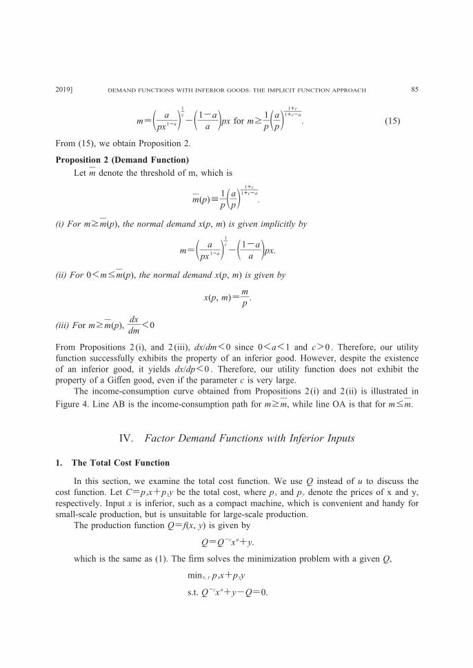
(iii) The limit of the second term of (17) is zero, since

limu−(aa

1a−a1

1a)⋅pxa1a⋅py

1

1a⋅Qc1a→0.

Then, the total cost curve converges to the straight line C=pyQ as q increases. Therefore,

the total cost curve is spoon-shaped and shown as TC in Figure 5.

Proposition 2(iii) means that although marginal cost is not constant, it converges to the constant

py . In this sense, C(Q) is a quasi-constant marginal cost. The reason is that when Q is

sufficiently large, the need for an inferior good almost vanishes. Production is carried out using

normal goods. In Q=Qcxa+y, the term y denotes the normal good and is the constant

marginal cost. The inferior good is used only when its marginal product per price is higher than

or equal to that of the normal good. If the inferior good is not available, we must only use the

normal good, which gives the total cost curve C=pyQ in Figure 5. Therefore, the depth of the

spoon represents the savings from the inferior good.

2. Extension to the Cobb-Douglas Production Function

In Q=Qcxa+y, the variable y is the simplest homothetic of degree 1 functions. Then, we

can replace y with y=βKzL1z, where K is capital, and L is labor. Furthermore, we add a

parameter, b. The production function Q(x, y) is given by

Q=b

Qcxa+βKzL1z (18)


Q

C=pyQ

A

C(Q)

O

TC

a

b

1－a＋ca

px

apy( )

The dotted straight line represents the TC curve when the inferior input is unavailable, and the spoon-shape TC curve

represents total cost when the inferior input is available. By using the inferior input, cost is reduced for a small

production level. The length of ab represents this cost saving.

FIGURE 5. TOTAL COST CURVE

where 0<b, 0<β, and 0<z<1.6

Total cost is pxx+rK+wL, where r is the rental rate, and w is wage. The firm solves the

minimization problem:

min x, K, L pxx+rK+wL

s.t Qcbxa+βYzL1z−Q=0.


ℒ=pxx+rK+wL−λb

Qcxa+βKzL1z−Q.

Then, the first order conditions (FOC) are:

ℒ x=px−λab

Qcxa1=0

ℒK=r−λβzKz1=0

ℒL=w−λβ(1−z)Lz=0

ℒ=b

Qcxa+βKzL1z−q=0.

From these FOCs, we obtain Proposition 4 and Proposition 5.7

Proposition 4 (Factor Demand)

Let Q denote the threshold of Q, which is given by

Q=Q(px, r, w)≡ab

1

a

βpx r

z z

w

1−z 1z

a

1ac

. (19)

(i) For Q≤Q, the factor demand functions are given by

x(px, r, w, Q)=ab

βpxQc⋅

r

z z

⋅w

1−z 1z

1

1a

, (20)

K(px, r, w, Q)=1

β z

r

w

1−z 1z

Q−b

Qc ab

βpxQc r

z z

w

1−z 1z

a

1a

, and (21)

L(px, r, w, Q)=1

β 1−z

w

r

z z

Q−b

Qc ab

βpxQc r

z z

w

1−z 1z

a

1a

. (22)


6 An inferior input is a problem of organization, technology, and strategy, rather than the physical property of the

input. For example, labor is an inferior input if it is used in the old production system that is harmful to the body, or

that is slavish. These old systems work well in the poor circumstance. However, these dangerous systems lose their

efficiency in large-scale production.7 The proofs of Proposition 4 and Proposition 5 are given in Appendix C.

(ii) For 0≤Q≤Q, the factor demand functions are given by

x(px, r, w, Q)=b1

a Q1ca ,

K(px, r, w, Q)=0, and

L(px, r, w, Q)=0.

Proposition 4(i) shows the interior solution. Proposition 4(ii) shows the corner solution. From

(20), we obtain ∂x/∂Q<0. Therefore, we can confirm that x is an inferior input. From (20)-

(22), we also obtain derivatives such as ∂x/∂r>0, ∂x/∂w>0, ∂L/∂w<0, and ∂K/∂r<0, which

are standard results due to a price change. However, ∂K/∂w and ∂L/∂r vary according to Q.

Proposition 5 (Cross-Price Effect)

(i) For Q≤Q<1

1−a 1a

1ac

⋅Q,

∂K(px, r, w, Q)

∂w<0 and

∂L(px, r, w, Q)

∂r<0

(ii) For 1

1−a 1a

1ac

⋅Q≤Q,

∂K(px, r, w, Q)

∂w≥0 and

∂L(px, r, w, Q)

∂r≥0.

Proposition 5 (i) implies that if Q is so small that Q≤Q≤1

1−a 1a

1ac

⋅Q, then capital

demand is decreasing in wage. Similarly, labor demand is decreasing in rental rate. The inferior

input is more suitable for production than the production system using K and L.

Yet, Proposition 5(ii) means that if Q is so large that (1/(1−a))1a

1ac⋅Q≤Q, then the cross

factor-price effects are negative and labor and capital are substitutes.Figure 6 shows the Q-K graph of K(px, r, w, Q). Let w1 and w2, (w1<w2), denote wages.

K1 shows the graph of K(px, r, w, Q). Point A1 represents Q(px, r, w1), and point B represents

(1/(1−a))1a

1ac⋅Q(px, r, w1).

If wage rises from w1 to w2, then A1 moves to A2, which represents Q(px, r, w2). Point A1

is located to the left of A2 since ∂Q(px, r, w)/∂w>0.

Proposition 5(i) means that K2 is drawn below K1 and to the left of point B. Proposition 5

(ii) means that K2 is drawn above K1 to the right of point B. K0 represents K(⋅, r, w, Q), theoriginal Cobb-Douglas function, where the inferior input is not available to the firm.


V. General Model

1. Formulation of the General Case

In this section, we examine the general model. Utility u(x, y) is now given by

u=b1uc1x1

a1+b2uc2x2

a2, (23)

with the budget constraint m=px1+x2, where 0<ai<1, 0<bi, 0<ci, 0<p, and m>0,

(i=1, 2). The net-utility function is

g(x1, u, m)=b1uc1x1

a1+b2uc2(m−px1)

a2−u=0. (24)

Let u be a constant. The partial derivative, ∂g/∂x1, is

g1(x1, u, m)=a1b1uc1x1

a11+a2b2uc2(m−px1)

a21(−p)=0 (25)

for 0≤x1≤m/p. In addition, we can confirm that

gu(x1, u, m)=−b1c1uc11x1

a1−b2c2uc21(m−px1)

a2−1<0,

gm(x1, u, m)=a2b2uc2(m−px1)

a21>0, and

g11(x1, u, m)=a1(a1−1)b1uc1x1

a12+a2(a2−1)b2uc2(m−px1)

a22(−p)

2<0.


QA1 A2 BO

K0

K2

K1

Capital Demand

K(Q)

The K0 straight line represents the factor demand curve with K (FDK) when the inferior input is not available for the

firm. If the firm uses the inferior input, then FDK shifts downward from K0 to K1. If the wage increases, K1 shifts to

K2. When Q is small, both K and L are substituted by x, rather than K substituting L. Therefore, FDK shift downward

to K2 for production range A1-B.

FIGURE 6. CROSS-PRICE EFFECT TO K

2. Compensated Demand

Let x1 minimize the expenditure m subject to g(x1, u, m)=0 with a fixed u . Since u is a

constant, the two equations

g(x1, u, m)=0

g1(x1, u, m)=0.

give the solution (x1*(u), m*(u)). Mathematically, if gm>0, then the solution x1

*(u) minimizes m,

and the other solution m*(u) is its minimized value. Therefore, from (24) and (25), we obtain

the compensated demand function, x1(p, u).8

Proposition 6 (Compensated demand)

(i) The compensated demand, x1(p, u), is given implicitly by

F(x1, u)≡b1uc1x1

a1+b2a2b2p

a1b1 a2

1a2

uc1a2c2

1a2 x1(1a1)

a2

1a2−u=0. (26)

(ii) x1(p, u)>0 for p>0 and u>0.

(iii) limu0 x1(p, u)→0.

(iv) Ifc1a2−c2

1−a2

>1, then limu x1(p, u)→0.

(v) Ifc1a2−c2

1−a2

≤1, then limu x1(p, u)→∞.

Property (ii) means that the solution is always interior for p>0 and u>0 . Thus, our

compensated demand function F(xi, u)=0 never yields a corner solution. Property (iii) means

that the income-consumption curve always stems from the origin. Property (iv) states that a

good with a large c1 is inferior when u is sufficiently large, but (iii) implies that it is a normal

good when u is small. The OA curve in Figure 7 is the income-consumption curve of case (iv).

Property (v) states that a good with a small c1 is a normal good for all levels of u . The OB

curve in Figure 7 is the income-consumption curve of case (v).

3. Normal Demand

Let x1 maximize u with a given m. Since m is a constant, (24) and (25),

g(x1, u, m)=0

g1(x1, u, m)=0,

gives the solution (x1*, u*) . Mathematically, if gu<0 holds, then the solution x1

* maximizes u,

and the other solution u* is its maximized value. Therefore, from (24) and (25), we obtain the

normal demand function x1(p, m).

Proposition 7 (Normal demand)


8 We can also obtain (26) by using the Lagrange function L=px1+x2+λ(b1uc1x1

a1+b2uc2x2

a2−u), instead of using

the net-utility function (24).

(i) Normal demand x1(p, m) is given implicitly by

D(x1, m)≡

b1 x11a1

(m−px1)1a2

a2b2p

a1b1 c1

c1c2

x1a1+b2 x1

1a1

(m−px1)1a2

a2b2p

a1b1 c2

c1c2

(m−px1)a2

− x11a1

(m−px1)1a2

a2b2p

a1b1 1

c1c2

=0. (27)

(ii) x1(p, m)>0 for p>0, and m>0.

Proposition 7(ii) means that our function always yields an interior solution.

4. A numerical Example for the Two-goods Model

In this subsection, we provide a numerical example for the two-good model.

Case. 1: Normal good case

Consider the following parameters:

c1=0.2, c2=0.1, a1=a2=0.9, and b1=b2=p=1.

The utility equation and budget constraint are

u=u0.2x10.9+u0.1x2

0.9 and (28)

m=x1+x2,

respectively. From (26), the compensated demand equation is given by:


x1

B

x2

O

A

The income-consumption Curve (ICC) is always positive both for x1 and x2. Additionally, it always starts from origin

point O. The OA curve is the ICC of Proposition 6 (iv). Both x1 and x2 are normal goods when income is low.

However, x1 changes into an inferior good as income increases. Curve OB is the ICC of Proposition 6(v). This shape of

the ICC is that of the normal model.

FIGURE 7. INCOME-CONSUMPTION CURVE

F(x1, u)=u0.2x1

0.9+u0.8x10.9−u=0,

which is solvable for u. The compensated demand for the good 1 is

x1(1, u)=u

u0.2+u0.9 1

0.9

,

which is a normal good becausedx1(u)

du>0.

From (27), we obtain the normal demand, x1(1, m), as

x1

m−x1 0.2

x10.9+

x1

m−x1 0.1

(m−x1)0.9−

x1

m−x1 1

=0. (29)

Table 1 shows the values of x1(1, m) calculated using a computer.9For m=5 and m=10 in

Table 1, the income elasticity isΔx

Δm

m

x=

1.31−1.05

10−5

5

1.05≑0.25<1. Thus, x1 is a necessary

good.

Case 2: Inferior good case

Consider the following parameters:

c1=0.3, c2=0.1, a1=a2=0.9, and b1=b2=p=1.

The utility equation and the budget constraint are

u=u0.3x10.9+u0.1x2

0.9 and (30)

m−x1−x2=0,

respectively. From (26), we have

F(x1, u)=u0.3x1

0.9+u1.7x10.9−u=0. (31)

Here, we can solve (31) for x1. Thus, we derive the compensated demand function as

x1(1, u)=u

u0.3+u1.7 1

0.9

. (33)

From (33), we have limu x1(1, u)→0. Therefore, x1 is an inferior good for large a u, as

discussed in Proposition 6(iv).

From (27), the normal demand function, x1(1, m) is implicitly given by


9 The program code for Table 1 and Table 2 is attached as “055Eq (27) Table1and2.xlsx” for Excel, or

“055Eq27CalculatorTwoGoods.m” for GNU octave. These programs are available upon a request.

0.490.44 0.72 0.85 1.05

0.3

1.31

0.8

1.58

1 2 3 5 10 20m

0.22

TABLE 1. THE TWO-GOODS MODEL (NORMAL GOODS)

x1

D(x1, m)=x1

m−x1 0.15

x10.9+

x1

m−x1 0.05

(m−x1)0.9−

x1

m−x1 0.5

=0. (34)

Table 5 shows the values of x1(m) calculated from (34).

From Table 2, we draw the Engel curve shown in Figure 8.

Figure 8 shows that good 1 is a normal good when m is small. However, as income

increases, demand stagnates, eventually decreasing to almost zero.

VI. Conclusion

Our function is so flexible that it can generate very various income-consumption curves as

shown in Figure 7. This flexibility is useful for analyzing the consumerʼs data. This paper

concentrates on the two-variable model. However, this function can be extended to the multi-

variable model. Using fully the implicit function may improve the researches in this fields

including Giffen Case in future, since the approach we use in this paper make the function

tractable and simple.

APPENDIX

A. Alternative Derivation of (7) and (15)

We derive x(p, u) and x(p, m) using the optimization technique of the implicit function. This


0 Income (:m)

B: case 2

Demand

x1A: case 1

Curve A is the Engel curve of the necessary good given by Eq (29), and curve B the Engel curve of an inferior good

given by Eq (34).

FIGURE 8. ENGEL CURVE

0.490.45 0.5 0.43 0.34

0.3

0.23

0.8

0.14

1 2 3 5 10 20m

0.26

TABLE 2. THE TWO-GOODS MODEL (INFERIOR GOODS)

x1

technique is an alternative to the Lagrange method for optimization of the implicit function.

Let the utility function and the budget constraint be10

u=bucxa+β, (A.1)

m=px+. (A.2)

From (A.1) and (A.2), by removing y, we obtain the in-budget utility as

g(x, u, m)≡bucxa+β(m−px)−u=0. (A.3)

Derivation of (7)

The expenditure m(x, u) is implicitly given by

g(x, u, m(x, u))=0

for a constant u.

Mathematically, m(x, u) is minimized if g(x, u, m)=0, gx=0, and gm≠0(>0). That is, the condition for

the minimization is:

g(x, u, m)=bucxa+β(m−px)−u=0, (A.4)

gx=abucxa1−βp=0, (A.5)

gm=β≠0(>0). (A.6)

From (A.4), we successfully obtain

x(u)= abβpuc 1a

. (A.7)

By removing the bar from u and setting β, b=1, (A.7) becomes (7).

Q.E.D.

Derivation of (15)

The utility u(x, m) is implicitly given by

g(x, u(x, m), m)=0

for a constant m.

Mathematically, the utility u(x, m) is maximized if g(x, u, m)=0, gx=0, and gu≠0(<0) . That is, the

condition for the maximization is:

g(x, u, m)=bucxa+β(m−px)−u=0, (A.8)

gx=abucxa1−βp=0, (A.9)

gu=−bcuc1xa−1≠0 (<0). (A.10)


10 In Appendix A, we use u and m to represent “a constant value,” although, in Appendix B and C, u and m are

reused as “the threshold value.” This duplication is only to reduce the variable.

From (A.9), we obtain

u=ab

βpx1a 1

c

. (A.11)

From (A.8) and (A.11), we obtain

bab

βpx1a 1

c

c

xa+β(m−px)−ab

βpx1a 1

c

=0

→m+1

a−1px−

ab

βpx1a 1

c

=0. (A.12)

By removing the bar from m and setting β, b=1, (A.12) becomes (12).

Q.E.D.

B. Proof of Proposition 3

Proof of Proposition 3(i) and (ii)

(a) Factor demand function

The firmʼs optimization problem is

min x, y pxx+pyy

s.t Qcbxa+β−Q=0.


ℒ=pxx+pyy−λb

Qcxa+β−Q. (B.1)

The first order condition is as follows:

ℒ x=px−λab

Qcxa1=0 (B.2)

ℒ y=py−λβ=0 (B.3)

ℒ=Q−b

Qcxa+β=0. (B.4)

From (B.2) and (B.3), we obtain

abQcxa1

px=

β

py

→xa1=β

abQc⋅px

py

→x=ab

βQc⋅py

px 1

1a

. (B.5)


From (B.4) and (B.5), the demand for y is

y=1

β Q−b

Qc ab

βQc⋅py

px a

1a

. (B.6)

In (B.6), y(Q) is positive only if

Q−b

Qc ab

βQc⋅py

px a

1a

≥0

→Q≥b

Qc ab

βQc⋅py

px a

1a

→Q⋅Qc⋅Qca

1a ≥bab

β⋅py

px a

1a

→Q1ac1a ≥b

ab

β⋅py

px a

1a

→Q1ac1a ≥

ab1

a

β⋅py

px a

1a

→Q≥ab

β⋅py

px 1a

1ac

≡Q(px, py). (B.7)

The formula Q≥Q(px, py) is the interior condition for y. From (B.5), (B.6), and (B.7), if Q≤Q(px, py),

then

y=0. (B.8)

Therefore, from (B.4) and (B.8), we obtain

Q−bQcxa+β⋅0=0

→x=b1

a Qc1

a . (B.9)

Summing up (B.5) and (B.9), we obtain the full statement of the factor demand function of

Q=Qcbxa+β as follows.

Factor Demand Function

The threshold level for the interior solution is

Q(px, py)≡ab

β⋅py

px 1a

1ac

. (B.10)

For Q≥Q(px, py),

x(px, py,Q)=ab

βQc⋅py

px 1

1a

, (B.11)


y(px, py,Q)=1

β Q−b

Qc ab

βQc⋅py

px a

1a

. (B.12)

For Q≤Q(px, py),

x(px, py,Q)=b1

a Qc1

a , (B.13)

y(px, py,Q)=0. (B.14)

(b) Total cost function

The total cost function for Q≥Q(px, py) is given by

C=px⋅x(px, py, Q)+py⋅y(px, py, Q)

→C=pxab

βQc⋅py

px 1

1a

+py1

β Q−b

Qc ab

βQc⋅py

px a

1a

→C=pxab

βQc⋅py

px 1

1a

+py1

βQ−py

1

β b

Qc ab

βQc⋅py

px a

1a

→C=pxa1

1ab

βQc 1

1a

py1

1apx1

1a+py1

βQ−py

1

β

b

Qc ab

βQc⋅py

px a

1a

→C=pxa1

1ab

βQc 1

1a

py1

1apx1

1a+py1

βQ−py

1

β

b

Qc ab

βQc a

1a

pya

1apxa1a

→C=a1

1ab

βQc 1

1a

py1

1apxa1a+py

1

βQ−

1

β

b

Qc ab

βQc a

1a

py1

1apxa1a

→C=a1

1ab

βQc 1

1a

py1

1apxa1a+py

1

βQ−a

a

1a1

β

b

Qc b

βQc a

1a

py1

1apxa1a

→C=a1

1ab

βQc 1

1a

py1

1apxa1a+py

1

βQ−a

a

1ab

βQc 1

1a

py1

1apxa1a

→C=py1

βQ−a

a

1a−a1

1ab

βQc 1

1a

py1

1apxa1a (B.15)

The total cost function for Q≤Q(px, py) is given by

C=px⋅x(px, py,Q)+py⋅y(px, py,Q)

→C=pxb

1

aQc1

a +py⋅0

→C=pxb1

a Qc1

a . (B.16)

Summing up (B.15) and (B.16), we obtain the full description of C(Q) as Q=Qcbxa+β, as follows.


Total Cost Function

For Q≥Q(px, py),

C(Q, px, py)=py1

βQ−a

a

1a−a1

1ab

βQc 1

1a

py1

1apxa1a. (B.17)

For Q≥Q(px, py),

C(Q, px, py)=pxb1

a Qc1

a . (B.18)

If b=1 and β=1, then (B.17) and (B.18) give (16) and (17).

Q.E.D.

Proof of Proposition 3(iii)

The term aa

1a−a1

1a⋅pxa1a⋅py

1

1a⋅Qc1a in (A6) is positive since 0<a<1.

The limit of this term is

limuaa

1a−a1

1a⋅pxa1a⋅py

1

1a⋅Qc1a→0.

Then, the total cost curve must be approaching the straight line C=pyQ as Q increases. Thus, the TC

curve is drawn below the dotted straight line labelled C=pyQ in Figure 5. The TC curve O-A-TC in

Figure 5 takes a spoon shape.

Q.E.D.

C. Proofs of Proposition 4 and Proposition 5

Proofs of Proposition 4(i)–(iii)


ℒ=pxx+rK+wL−λb

Qcxa+βKzL1z−Q. (C.1)

The FOC is

ℒ x=px−λab

Qcxa1=0, (C.2)

ℒK=r−λβzKz1=0, (C.3)

ℒL=w−λβ(1−z)Lz=0, (C.4)

ℒ=Q−b

Qcxa+βKzL1z=0. (C.5)

From (C.3) and (C.4), we obtain

K=z

r

w

1−zL (C.6a)

or


L=r

z

1−z

wK. (C.6b)

From (C.2) and (C.3) we obtain

ab

pxQcx

a1=(1−z)

wβKzLz. (C.7)

From (C.6a) and (C.7), we obtain

ab

pxQcx

a1=(1−z)

wβz

r

w

1−zL

z

Lz. (C.8)

By solving (C.8) for x, we obtain

x(px, r, w, Q)=ab

βpxQc⋅

r

z z

⋅w

1−z 1z

1

1a

. (C.9)

From (C.5), (C.6b), and (C.9), we obtain

K(px, r, w, Q)=1

β z

r

w

1−z 1z

Q−b

Qc ab

βpxQc r

z z

w

1−z 1z

a

1a

. (C.10)

From (C.5), (D6a), and (C.9),

L(px, r, w, Q)=1

β 1−z

w

r

z z

Q−b

Q c ab

βpxQc r

z z

w

1−z 1z

a

1a

. (C.11)

(C.9)‒(C.11) give (20)‒(22), respectively.

The value of K(px, r, w, Q) and L(px, r, w, Q) shown in (C.10) and (C.11) must be non-negative for

Q≥0. From (C.10), K(px, r, w, Q)≥0 if

0≤Q−b

Qc ab

βpxQc r

z z

w

1−z 1z

a

1a

→b1aa ⋅

ab

βpx r

z z

w

1−z 1z

≤Q (c1)1aa

c

→Q(px, r, w)≡ab1

a

βpx r

z z

w

1−z 1z

c

1ac

≤Q. (C.12)

The LHS of (C.12) is denoted as Q(px, r, w) in (19). Therefore, we obtain the interior condition of K as

Q(px, r, w)≤Q. (C.13)

Similar calculation to (C11)‒(C.13) gives L(px, r, w, Q)≥0 for (C.13).

(C.13) is used in Proposition 4(i).

Q.E.D.


Proof of Proposition 4(ii)

If 0≤Q≤Q, K(px, r, w, Q)=0, and L(px, r, w, Q)=0, then the production function is simply the single

variable function Q=bQcxa. Solving this for u, we obtain x(px, r, w, Q)=b1

a Q1ca . Therefore, we obtain

(ii).

Q.E.D.

Proof of Proposition 5(i)

By removing the curly braces from (C.10), for Q<Q, we obtain

K(px, r, w, Q)=1

β z

r

w

1−z 1z

Q−1

β z

r

w

1−z 1z

⋅b

Q c ab

βpxQc r

z z

w

1−z 1z

a

1a

. (C.14)

The differentiation of (C.14) for w is negative if

∂K

∂w=

1

β z

r

w

1−z 1z

Q(1−z)w1−1

β z

r

w

1−z 1zb

Qc ab

βpxQc r

z z

w

1−z 1z

a

1a

(1−z)1

1−aw1<0,

which is rewritten as

1

β z

r

w

1−z 1z

Q(1−z)w1<1

β z

r

w

1−z 1zb

Yc ab

βpxQc r

z z

w

1−z 1z

a

1a

(1−z)1

1−aw1.

(C.15)

In the variables of (C.15), three terms1

β z

r

w

1−z 1z

, (1−z), and w1 appear on both the LHS and RHS.

Thus, we can remove these from (C.15). Therefore, (C.15) is now

Q<b

Qc ab

βpxQc r

z z

w

1−z 1z

a

1a 1

1−a(C.16)

→Q<1

Qc 1

Qc a

1a

bab

βpx r

z z

w

1−z 1z

a

1a 1

1−a

→Q1cca

1a<bab

βpx r

z z

w

1−z 1z

a

1a 1

1−a

→Q<ab1

a

βpx r

z z

w

1−z 1z

a

1ac

1

1−a 1a

1ac

→Q<Q⋅1

1−a 1a

1ac

. (C.17)

From (C.14)‒(C.17), we successfully obtain

∂K(px, r, w, Q)

∂w<0 for Q≤Q<

1

1−a 1a

1ac

⋅Q. (C.18)


A similar calculation to (C.14)‒(C.17) gives

∂L(px, r, w, Q)

∂r<0 for Q≤Q<

1

1−a 1a

1ac

⋅Q. (C.19)

Q.E.D.


By changing the inequality “<” of (C.14)‒(C.17) by “≥,” we obtain

∂K(px, r, w, Q)

∂w≥0 for

1

1−a 1a

1ac

⋅Q≤Q.

A similar calculation to (C.14)‒(C.17) gives

∂L(px, r, w, Q)

∂r≥0 for

1

1−a 1a

1ac

⋅Q≤Q.

Q.E.D.

D. Proof of Proposition 6


From (25), we obtain

g1(x1, u, m)=a1b1uc1x1


a21(−p)=0

→a1b1uc1x1


a21(−p)=0

→m−px1=a1b1u

c1

a2b2puc2x1a11

1

a21

. (D.1)

From (24) and (D.1), we obtain

g(x1, u, m)=b1uc1x1

a1+b2uc2(m−px1)

a2−u=0

→b1uc1x1

a1+b2uc2

a1b1uc1x1

a11

a2b2puc2

a2

a21

−u=0

→F(x1, u)≡b1uc1x1

a1+b2a2b2p

a1b1 a2

1a2

uc1a2c21a2 x1

(1a1)a2

1a2−u=0. (D.2)

(D.2) is (26).


We must prove that x1(p, u)>0 for p>0 and u>0.

Let us decompose (D.2) into two functions, LHS and RHS, where

LHS(x1, u)=b1uc1x1

a1+b2a2b2p

a1b1 a2

1a2

uc1a2c21a2 x1

(1a1)a2

1a2, and


RHS(x1, u)=u.

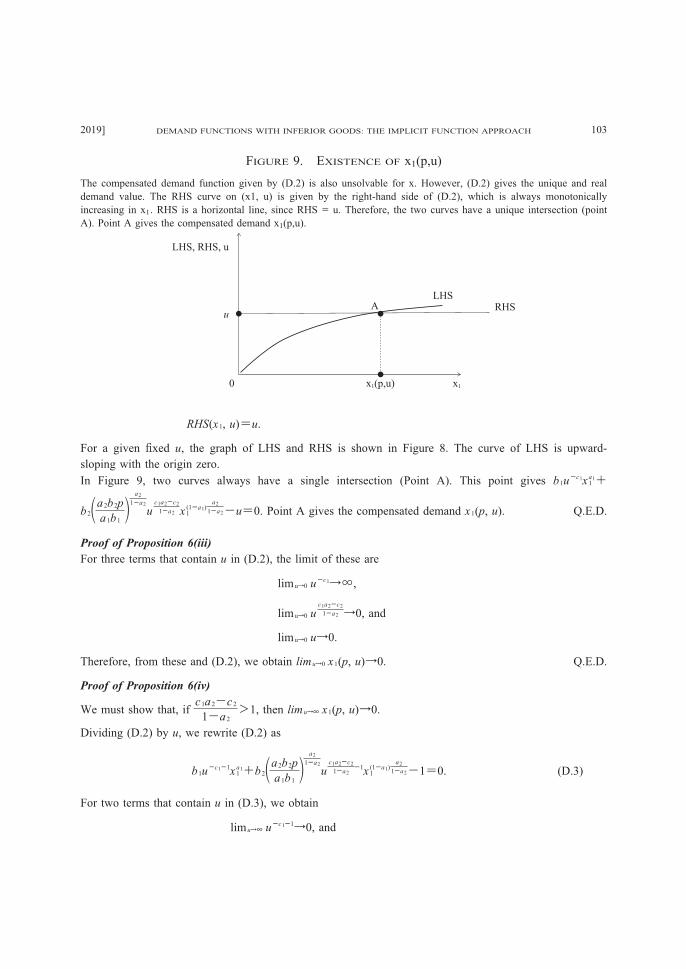
For a given fixed u, the graph of LHS and RHS is shown in Figure 8. The curve of LHS is upward-

sloping with the origin zero.

In Figure 9, two curves always have a single intersection (Point A). This point gives b1uc1x1

a1+

b2a2b2p

a1b1 a2

1a2

uc1a2c21a2 x1

(1a1)a2

1a2−u=0. Point A gives the compensated demand x1(p, u). Q.E.D.

Proof of Proposition 6(iii)

For three terms that contain u in (D.2), the limit of these are

limu0 uc1→∞,

limu0 uc1a2c21a2 →0, and

limu0 u→0.

Therefore, from these and (D.2), we obtain limu0 x1(p, u)→0. Q.E.D.

Proof of Proposition 6(iv)

We must show that, ifc1a2−c21−a2

>1, then limu x1(p, u)→0.

Dividing (D.2) by u, we rewrite (D.2) as

b1uc11x1

a1+b2a2b2p

a1b1 a2

1a2

uc1a2c21a2

1x1(1a1)

a2

1a2−1=0. (D.3)

For two terms that contain u in (D.3), we obtain

limu uc11→0, and


0 x1(p,u)

uRHS

LHSA

LHS, RHS, u

x1

The compensated demand function given by (D.2) is also unsolvable for x. However, (D.2) gives the unique and real

demand value. The RHS curve on (x1, u) is given by the right-hand side of (D.2), which is always monotonically

increasing in x1. RHS is a horizontal line, since RHS = u. Therefore, the two curves have a unique intersection (point

A). Point A gives the compensated demand x1(p,u).

FIGURE 9. EXISTENCE OF x1(p,u)

limu uc1a2c2

1a21→∞ ∵

c1a2−c2

1−a2

>1 .Therefore, from these and (D.3), we obtain limu x1(p, u)→0 Q.E.D.

Proof of Proposition 6(v)

We must show that, ifc1a2−c2

1−a2

≤1, then limu x1(p, u)→∞.

The compensated demand x1 must hold (D.3). For the two terms that contain u in (D.3), we obtain

lim uc11→0, and

limu uc1a2c2

1a21→0 ∵

c1a2−c2

1−a2

<1 .Therefore, from these and (D.3), x1 must be an infinite. Then, we obtain limu xi(p, u)→∞. Q.E.D.

E. Proof of Proposition 7


From (25), for c1≠c2, we obtain

aibi

a2b2pucic2x1

ai11

a21

=m−px1 (E.1)

→u=x11a1

(m−px1)1a2

a2b2p

a1b1 1

c1c2

. (E.2)

By substituting (E.2) into (24), we obtain

b1x11a1

(m−px1)1a2

a2b2p

a1b1 c1

c1c2

x1a1+b2

x11a1

(m−px1)1a2

a2b2p

a1b1 c2

c1c2

(m−px1)a2−

x11a1

(m−px1)1a2

a2b2p

a1b1 1

c1c2

=0

(E.3)

Equation (E.3) is (27). Q.E.D.


We must show that (E.3) always gives x1(p, m) as a positive real number.

We rewrite (E.3) as

b1x11a1

(m−px1)1a2

a2b2p

a1b1 c1

c1c2

x1a1+b2

x11a1

(m−px1)1a2

a2b2p

a1b1 c2

c1c2

(m−px1)a2=

x11a1

(m−px1)1a2

a2b2p

a1b1 1

c1c2

.

(E.4)

Figure 10 shows the case of c1<c2. This implies−c1

−c1+c2

<0,−c2

−c1+c2

<0, and1

−c1+c2

>0. In Figure

10, the R curve represents the RHS of (E.4). On the other hand, the L1+2 curve represents the LHS of

(E.4).11 At point E, the RHS is equal to the LHS. Then, both x1* and u* are given by E. If m increases,

then point A moves to the right. Thus, point E moves either left or right. Q.E.D.


REFERENCES

Doi, J., K. Iwasa and K. Shinomura (2009), “Giffen Behavior Independent of the Wealth

Level”, Economic Theory, 41, pp. 247-267.

Epstein, G. S. and U. Spiegel (2000), “A production Function with an Inferior Input”, The

Manchester School 68, pp.503-515.

Moffatt, P.G. (2002), “Is Giffen Behaviour Compatible with the Axioms of Consumer Theory?”,

Journal of Mathematical Economics, 37, pp.259-267.


11 The L2 curve in Figure 10 represents the second term of the LHS. Although L2 is drawn as a concave curve, it is

not always like this. Depending on a1, a2, c1, and c2, the L2 curve can be an upward-sloping curve. However, regardless

of whether it is concave or upward-sloping, L1+2 remains an upward-sloping curve.

x1

L, R

x1*

E

A

L1+2

R

0

pm

The L1+2 curve represents the sum of the first and second terms of the left-hand side of (E.4), whose value is [0, ∞).

The R curve represents the right-hand side of (E.4), whose value is [0, ∞) and is increasing in x1. Point E gives the

demand for x1. If m increases, then point A shifts to the right.

FIGURE 10. NORMAL DEMAND

Documents

DEMANDFUNCTIONSWITHINFERIOR GOODS: THE IMPLICIT