Demand Systems in Industrial Organization: Part I∗

John Asker

January 3, 2017

1 Overview

Demand systems often form the bedrock upon which empirical work in industrial organizationrests. The next few lectures aim to introduce you to the different ways empirical researchers haveapproached the issue of demand estimation in the applied contexts that we typical confront as IOeconomists. I will start by briefly overviewing the types of research questions and various instancesin which demand estimation is useful, and the core problems we face when estimating demand.

We will begin with a basic overview of homogeneous product market competition (with whichyou should be familiar), and an overview of estimation in these markets. We will then move tomodels of differentiated product demand systems. I will review basic theory and standard dataforms, after which I will go on to talk about the standard approaches to demand estimation andtheir advantages and disadvantages. All these approaches try to deal with the problem of estimatingdemand when we are in a market with many, differentiated goods. Specific papers will be used toillustrate the techniques once they have been discussed.

I will expect you to remember your basic econometrics, particularly the standard endogeneityproblem of estimating demand (see Working 1927 or the treatment in standard econometrics texts,e.g. Hayashi 2000 in Ch 3).

There has been an explosion in the sophistication of technique used in demand estimation thelast decade, due to a combination of advances in econometric technique, computation and dataavailability.

1.1 Why spend time on Demand Systems?

Many questions in IO require understanding how consumers choose among various goods and ser-vices as a function of market and individual characteristics. Though properly estimating a demandsystem in its own right may be an objective of interest, demand systems (and their underlyingparameters) are more often than not used as an input into answering other, perhaps larger, ques-tions. E.g., they are often used as providing the incentives for examining firm behavior (pricing,investment, product introduction, entry/exit, etc...), or computing consumer welfare from a policychange. For example...

• Infer firm conduct: sometimes it is difficult to observe/measure firm conduct directly, butwe might be able to test certain theories by using consumer demand estimates to infer firmbehavior.

∗These notes draw from a variety of sources: in particular Ariel Pakes’ lecture notes, and from (co-teaching with)Robin Lee and Allan Collard-Wexler.

1

– Example: Bresnahan 1987 Competition and Collusion in 1950s Auto Market

Bresnahan wanted to examine the hypothesis that the dramatic increase in quantity(45% greater than in two surrounding years) and decrease in the price of Autos in 1955was due to the temporary breakdown of a collusive agreement. Unlikely to be demandshock: “any explanation of all of the 1955 events from the demand side will need to befairly fancy.”

His idea was to assume that marginal costs were not varying and then ask whether therelationship between pricing and demand elasticities changed in a manner consistentwith a shift from collusion to oligopolistic pricing.

He exploits data on P and Q for different makes of automobiles. He has about 85 modelsover 3 years. The “magic” in these approaches is using demand data combined with anequilibrium assumption on firm conduct to back out marginal costs, without using anycost data. We’ll come back to this later.

• Welfare impacts: to conduct welfare calculations subsequent to some market change broughtabout by, say, policy intervention, product introduction, or etc., one needs a well specifieddemand system. It allows us to quantify the “Value of Innovation”: e.g., compute consumer

2

surplus from the introduction of a new good (e.g., minivans, CAT scans) with similar “char-acteristics” of existing ones.

• Determinants of Innovation: with a demand system, a researcher can compute predictedmarkups for a given good; consequently, one will understand the types of products a firmwill want to produce (e.g., minivans or SUV’s, cancer drugs instead of malaria treatments).Demand systems, in other words, help us measure the incentives for investing in new goods.

• Usually demand is important to think about various forms of comparative statics: commonones for IO researchers include pre and post merger pricing, tax incidence, monopoly vsduopoly pricing, effect of predatory pricing policies, impact of new product introductions,etc.

• In IO and Marketing, there is considerable work on advertising which usually involves somedemand estimation. This about policy questions of direct-to-consumer drug adverting, oradvertising as a barrier to entry. Furthermore, carefully specified demand systems can assistwith decomposing the mechanisms or channels through which various advertising (and other)effects work. E.g., persuasive vs. informative advertising.

• Understanding the cross-price elasticities of good is often crucial to “preliminary” issues inpolicy work, such as market definition in antitrust cases. Also, they inform determinantsof market power: should we allow two firms to merge? Is there collusion going on in thisindustry (unusually large markups)? Cross-price elasticities are one input into this equation.(We will talk a bit (later) about the myriad antitrust applications of demand models. Notethat this is the largest consumer of Ph.D’s in Empirical I.O. by a long shot!)

• The tools used in demand estimation are starting to be applied in a variety of other contexts(e.g., political economy, development, education, health...) to confront empirical issues, ofthere is likely to be some intellectual arbitrage for your future research.

2 Approaches to demand estimation

Approaches breakdown along the following lines:

• single vs multi-products

• within multi-product: whether you use a product space or characteristic space approach

• representative agent vs heterogenous agent

• Other breakdowns: continuous vs. discrete choice, horizontal vs. vertical, dynamic vs.static...

We will primarily focus on multi-product, demand systems with heterogeneous agents. We willcover both product and characteristics space approaches. We will focus on static settings, and laterdiscuss methods for dealing with dynamics.

3

3 On Demand Estimation

3.1 Data... (briefly)

As always, the credibility and success of empirical work will hinge on the data that is leveraged.Depending on the industry and the application, data may be plentiful or sparse; it is alwayspreferable to rely on richer data (when availabile and accessible at reasonable cost (both time andfinancial)) to inform our estimates than to implicitly assume them through structure or assumptions.That said, research is all about navigating these tradeoffs (and being explicit and honest aboutthem).

To anchor discussion, the data that we should have in mind when discussing demand estimationtends to look as follows:

• The unit of observation will be quantity of product purchased (say 12 oz Bud Light beer)together with a price for a given time period (say a week) at a location (Store, ZIP, MSA,state, country...).

• You will generally need to take a stance on the relevant market and set of products withina consumer’s choice set; in addition, there typically is an outside good (e.g., non purchase)that you will need to control for (either with data or via assumptions).

• There is now a large amount of consumer-level purchase data collected by marketing firms(for instance the ERIM panel used by Ackerberg RAND 1997 to look at the effects of TVads on yogurt purchases). However, the vast majority of demand data is aggregated at somelevel. As we will discuss, less-aggregated data tends to allow us to estimate more detailed(ambitious) models.

• Note that you often have a lot of information: you can get many characteristics of the good(Alcohol by volume, calories, etc) from the manufacturer or industry publications or packagingsince you know the brand. The location means we can merge the demand observation withcensus data to get information on consumer characteristics. The date means we can look atsee what the spot prices of likely inputs were at the time (say gas, electricity etc).

• Typical data sources: industry organizations, marketing and survey firms (e.g. AC Nielson),proprietary data from manufacturer, marketing departments have some scanner data online(e.g. Chicago GSB).

• The survey of consumer expenditures also has some information on person-level consumptionon product groups like cars or soft-drinks.

• More often than not, data will require some ingenuity, luck, and a lot of elbow grease to obtain.Theory can help fill in some holes, but at the end of the day, good data (and variation!) isnecessary for a convincing paper.

3.2 Basics: Endogeneity of Prices and Other Definitions

Consider a market equilibrium in a competitive market with the following components:

4

Aggregate Demand. Say it takes a constant elasticity form, i.e.

ln(Qn) = xnβ − αln(pn) + εn

where n indexes markets, x are observed and ε are unobserved (by the econometrician) factorsthat cause differences in demand at a given price. E.g.,: parameters of income distribution, priceof substitutes or complements, environmental factors that cause differences in the demand for thegood,...

Aggregate supply.mcn = wnγ + λQn + ωn

w are observed and ω are unobserved (by the analyst) factors that cause differences in marginalcost. The marginal cost curve is the marginal cost of the market maker; it need not be the truesocial marginal cost.

Equilibrium. We assume the market is in equilibrium, i.e. demand=supply, or that the auction-eer sets price at a level where the quantity it induces equates demand and supply

pn = mcn.

Note that under an auctioneer interpretation, this assumes that he knows (ε, ω) even Moregenerally there often are variables that are either observed to all agents, or revealed while findingthe equilibrium price, that we do not contain good measures of in our data sets.

Keep in mind that:

• if there are differences in ε or in ω that are not known by the ”auctioneers” (i.e. not incor-porated in price) then there can be excess demand or supply. You can introduce that intoyour model, but you need a way of dealing with it. In many markets you could introduceinventories (though then you might want to add dynamics) or a rationing system. One of theimportant facts about electricity generation is that it is very hard (though not impossible)to store energy, and this rules out inventories. What the market maker does in electricitygeneration is have a special reserve market where the ISO pays a “holding” fee to generators,and can bring them up or down from a central computer to make sure the market balancesat all times.

• we have simplified by assuming that last period’s price does not effect either marginal cost ordemand (in keeping within the simple static framework). As noted in the first lecture thereare many reasons why it might, but this would put us into a world where demand or supplytoday depends on past, and perceptions of future, prices. I.e. a world where to analyze thedeterminants of current price and quantity determinants we need dynamics.

3.3 Single Product Demand Estimation

Let’s now move away from competitive markets, and abstract from the supply side for a moment.

5

• Begin with one homogenous product. Assume demand for product j in market t could begiven by qjt = D(pjt, Xj,t, ξjt), where qjt are quantities, pjt are prices, Xjt are exogenousvariables, and ξjt are random shocks.

• Let’s assume now demand is iso-elastic:

ln(qjt) = αj ln pjt +Xjtβ + ξjt (1)

so that price elasticity ηjt = αj . Xjt could just be an intercept for now (constant term) or avector of demand shifters. ξjt is a one-dimensional unobserved component of demand.

Problem 1: Endogeneity of Prices

Recall from the monopoly discussion that we might be interested in price elasticities: doing sowould allow us to use theory to perhaps recover (“infer”) marginal cost by simply observing theprice charged in a market.

• Suppose we are in a situation where the error term ξjt is correlated with higher prices (pjt),i.e. E(ξjtpjt) > 0.

• Let’s decompose this correlation into:

ξjt = λpjt + εjt

where εjt is the remaining uncorrelated part, and λ will typically be positive. Then we can put thisback in:

ln(qjt) = αjpjt +Xjtβ + ξjt

= αjpjt +Xjtβ + λpjt + εjt

= (αj + λ)︸ ︷︷ ︸α̂j

pjt +Xjtβ + εjt

So the coefficient that we estimate denoted α̂j will be biased upwards. This will lead to unrealis-tically low estimates of price elasticity. We call this the simulataneity problem. The simultaneity(or endogeneity) problem is a recurrent theme in Empirical I.O.

• In I.O. we almost never get experimental or quasi-experimental data.

• Unlike what you’ve been taught in econometrics, we need to think very hard about what goesinto the “unobservables” in the model (try to avoid the use of the word error term, it maskswhat really goes into the ε’s in I.O. models).

• Finally, it is a very strong assumption to think that the firm does not react to the unobservablebecause it does not see it – just because I don’t have the data doesn’t mean a firm doesn’t!

• Remember that these guys spend their lives thinking about pricing.

• Moreover, won’t firms react if they see higher than expected demand yesterday?

• Note: From here on, when you are reading the papers, think hard about “is there an endo-geneity problem that could be generating erroneous conclusions, and how do the authors dealwith this problem?”

6

3.3.1 Some History.

• Henry Moore (1914)’s O.L.S. analysis of quantity on price (an attempt to estimate demandcurves). Finds

– Demand curves for agricultural products sloped down

– Demand curves for manufacturing products sloped up.

• Working’s(1927) pictures. How do we connect equilibrium dots?

Figure 1: Working (1929 QJE)

• Needed assumption for O.L.S. on demand: E[ε|x, p] = 0, or even E[ε(x, p)] = 0 contradictsmodel and common sense (at least if the auctioneer or the firm that is pricing knows ordiscovers ε). I.e. for this to be true there is nothing that affects demand that the auctioneerknows that the empirical analyst does not know.

• Similarly needed equation for ”supply” or price curve contradicts model

• Solve for price and quantity as a function of (x,w, ω, ε).

• Possible Solutions:

– Estimation by 2SLS,

– Estimation by covariance restrictions between the disturbances in the demand and supplyequation.

See any standard textbook, e.g. Goldberger(1991).

7

Lesson. Thought should be given to what is likely to generate the disturbances in our models,and given that knowledge we should try to think through their likely properties.

Review: What is an instrumental variable

The broadest definition of an instrument is as follows, a variable Z such that for all possible valuesof Z:

Pr[Z|ξ] = Pr[Z|ξ′]

But for certain values of X we have

Pr[X|Z] 6= Pr[X|Z ′]

This second part makes it an instrumental variable.So the intuition is the Z is not affected by ξ, but has some effect on X. The usual way to

express these conditions is that an instrument is such that: E[Zξ] = 0 and E[XZ] 6= 0.

quantity demanded in response to a percentage change in price—first usingordinary least squares and then using instrumental variables with stormy weather asan instrument. In the regressions, fish has been treated as an approximatelyhomogeneous product. The first column is an ordinary least squares regressionwith log quantity as the dependent variable and log price as the independentvariable. The quantity is the total amount sold on a day and the price is the averageprice for that day.3 A higher price has a negative effect on quantity. The secondcolumn shows that this estimate is unchanged by including dummy variables for theday of the week (Friday is the omitted day), and for measures of the weather onshore.

The third column then uses an instrumental variables approach. That is, firsta regression is run with log price as the dependent variable and the storminess ofthe weather as the explanatory variable. This regression seeks to measure thevariation in price that is attributable to stormy weather. The coefficients from thisregression are then used to predict log price on each day, and these predictedvalues for price are inserted back into the regression. The third column shows thatthe impact of these predicted values of price on quantity are double the ordinary

3 There does not appear to be any correlation between stormy weather and the quality of whiting sold.

Table 2Ordinary Least Squares and Instrumental Variable Estimates of DemandFunctions with Stormy Weather as an Instrument

Variable

Ordinary least squares(dependent variable:

log quantity)Instrumental

variable

(1) (2) (3) (4)

Log price �0.54 �0.54 �1.08 �1.22(0.18) (0.18) (0.48) (0.55)

Monday 0.03 �0.03(0.21) (0.17)

Tuesday �0.49 �0.53(0.20) (0.18)

Wednesday �0.54 0.58(0.21) (0.20)

Thursday 0.09 0.12(0.20) (0.18)

Weather on shore �0.06 0.07(0.13) (0.16)

Rain on shore 0.07 0.07(0.18) (0.16)

R 2 0.08 0.23No. of Obs. 111 111 111 111

Source: The data used in these regressions are available by contacting the author.Note: Standard errors are reported in parentheses.

216 Journal of Economic Perspectives

Figure 2: Graddy (2006 JEP)

3.4 Multi-product Systems

Now let’s think of a multiproduct demand system to capture the fact that most products havesubstitutes for each other. Generally this would be given by the relationship

q = D(p,X, ξ)

8

where q,p, ξ are J × 1 vectors of quantities, prices, and random shocks, and X are exogenousvariables. We can follow the same approach before and assume that demand takes the followingisoelastic form:

ln q1 =∑j∈J

γ1j ln p1t + βx1t + ξ1t

...

ln qJ =∑j∈J

γJj ln pJt + βxJt + ξJt

3.4.1 Product vs Characteristic Space

We can think of products as being:

• a single fully integrated entity (a lexus SUV); or

• a collection of various characteristics (a 1500 hp engine, four wheels and the colour blue).

It follows that we can model consumers as having preferences over products, or over charac-teristics.

The first approach embodies the product space conception of goods, while the second embodiesthe characteristic space approach (see Lancaster (1966, 75, 79)).

Product Space: disadvantages for estimation

[Note that disadvantages of one approach tend to correspond to the advantages of the other]

• Dimensionality: if there are J products then we have in the order of J2 parameters to estimateto get the cross-price effects alone (the γjk terms above).

– Can get around this to some extent by imposing more structure. For example, onecan use functional form assumptions on utility: this leads to ”grouping” or ”nesting”approaches whereby we group products together and consider substitution across andwithin groups as separate things - means that ex ante assumptions need to be made thatdo not always make sense. More on this later.

– Can also impose symmetry: e.g., CES demand of J products with utility given by:

U(q1, . . . , qJ) = (

J∑i=1

qρi )1/ρ (2)

yields demand for good k:

qk =p−1/(1−ρ)k∑J

i=1 p−ρ/(1−ρ)i

I (3)

where I is the income for the consumer. Note now only have to estimate ρ as opposed tonumber of parameters proportional to J2. However, note this model implies:

∂qi∂pj

pjqi

=∂qk∂pj

pjqk

∀i, k, j (4)

9

which means all goods i and k have the same cross-price elasticities with respect to goodj. This is an extremely strong assumption, and imposes strong restrictions on the demandsystem. Though popular for analytic tractability, it is not generally used in empirical IO.

• Product space methods are not well suited to handle the introduction of new goods prior totheir introduction (consider how this may hinder the counterfactual exercise of working outwelfare if a product had been introduced earlier - see Hausman on Cell Phones in BrookingsPapers 1997 - or working out the profits to entry in successive stages of an entry game...)

Characteristic Space: disadvantages for estimation

• getting data on the relevant characteristics may be very hard and dealing with situationswhere many characteristics are relevant

• this leads to the need for unobserved characteristics and various computational issues indealing with them.

• dealing with new goods when new goods have new dimensions is hard (consider the introduc-tion of the laptop into the personal computing market)

• dealing with multiple choices and complements is a area of ongoing research, currently alimitation although work advances slowly each year.

We will explore product space approaches and then spend a fair amount of time on the char-acteristic space approach to demand. Most recent work in methodology has tended to use acharacteristics approach and this also tends to be the more involved of the two approaches.

4 Product Space Approaches: AIDS Models

I will spend more than an average amount of time on AIDS (Almost Ideal Demand System (Deatonand Mueller 1980 AER), which wins the prize for worst acronym in all of economics models), whichremain the state of the art for product space approaches. Moreover, AIDS models are still thedominant choice for applied work in things like merger analysis and can be coded up and estimatedin a manner of days (rather than weeks for characteristics based approaches). Moreover, the AIDSmodel shows you just how far you can get with a “reduced-form” model, and these less structuralmodels can fit the data much better than more structural models in some applications.

The main disadvantage with AIDS approaches, is that when anything changes in the model(more consumers, adding new products, imperfect availability in some markets), it is difficult tomodify the AIDS approach to account for this type of problem.

• Starting point for dealing with multiple goods in product space:

ln qj = αpj + βpK + γxj + εj

• What is in the unobservable (εj)?

– anything that shifts quantity demanded about that is not in the set of regressors

10

– Think about the pricing problem of the firm ... depending on the pricing assumptionand possibly the shape of the cost function (e.g. if constant cost and perfect comp,versus differentiated bertrand etc) then prices will almost certainly be endogenous. Inparticular, all prices will be endogenous.

– This calls for a very demanding IV strategy, at the very least

• Also, as the number of products increases the number of parameters to be estimated will getvery large, very fast: in particular, there will be J2 price terms to estimate and J constantterms, so if there are 9 products in a market we need at least 90 periods of data!

The last point is the one to be dealt with first, then, given the specification we can thinkabout the usual endogeniety problems. The way to reduce the dimensionality of the estimationproblem is to put more structure on the choice problem being faced by consumers. This is done bythinking about specific forms of the underlying utility functions that generate empricially convenientproperties. (Note that we will also use helpful functional forms in the characteristics approach,although for somewhat different reasons)

The usual empirical approach is to use a model of multi-level budgeting1:

• The idea is to impose something akin to a “utility tree”

– steps:

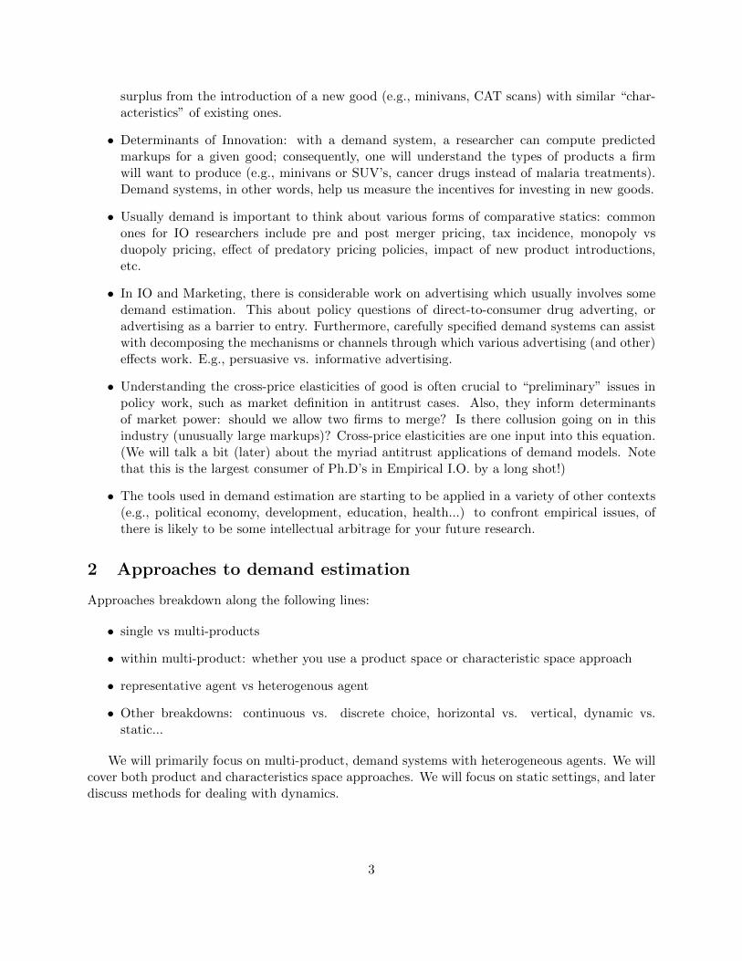
1. group your products together is some sensible fashion (make sure you are happy tobe grilled on the pros and cons of whatever approach you use). In Hausmann et al,the segments are Premium, Light and Standard.

2. allocate expenditures to these groups [part of the estimation procedure].

3. allocate expenditures within the groups [again, part of the estimation procedure]:Molson, Coors, Budweiser and etc...

Dealing with each step in reverse order:

1Note also that this is useful in other contexts - see for instance Fanyin Zhengs use of this, in her 2015 Job MarketPaper, in a dynamic entry game to ease computational burdens and capture some of the reality of the data generatingprocess.

11

3. When allocating expenditures within groups it is assumed that the division of expenditurewithin one group is independent of that within any other group. That is, the effect of a pricechange for a good in another group is only felt via the change in expenditures at the group level.If the expenditure on a group does not change (even if the division of expenditures within it does)then there will be no effect on goods outside that group.

2. To be allocate expenditures across groups you have to be able to come up with a price indexwhich can be calculated without knowing what is chosen within the group.

These two requirements lead to restrictive utility specifications, the most commonly used beingthe Almost Ideal Demand System (AIDS) of Deaton and Muellbauer (1980 AER).

4.1 Overview

This comes out of the work on aggregation of preferences in the 1970s and before. (Recall Chapter5 of Mas-Colell, Whinston and Green)

Starting at the within-group level: assume expenditure functions for utility u and price vectorp look like

log(e(u, p) = (1− u) log(a(p)) + u log(b(p))

where it is assumed:

log(a(p)) = α0 +∑k

αk log pk +1

2

∑k

∑j

γ∗kj log pk log pj (5)

log(b(p)) = log(a(p)) + β0Πkpβkk (6)

Using Shepards Lemma we can get shares of expenditure within groups as:

wi =∂log(e(u, p))

∂ log pi= αi +

∑j

γij log (pj) + βi log( xP

)where x is total expenditure on the group, γij = 1

2(γ∗ij + γ∗ji), P is a price index for the group andeverything else should be self explanatory.

Dealing with the price index can be a pain. It can be thought of as a price index that “deflates”income. There are two ways that are used. One is the ”proper” specification

log (P ) = α0 +∑k

αk log (pk) +1

2

∑j

∑k

γkj log (pk) log (pj)

which is used in the Goldberg paper, or a linear approximation (as in Stone 1954) used by most ofthe empirical litterature:

log (P ) =∑k

wk log (pk)

Deaton and Muellbauer go through all the micro-foundations in their AER paper.For the allocation of expenditures across groups you just treat the groups as individual goods,

with prices being the price indexes for each group. Again, note how much depends on the initialchoice about how grouping works.

12

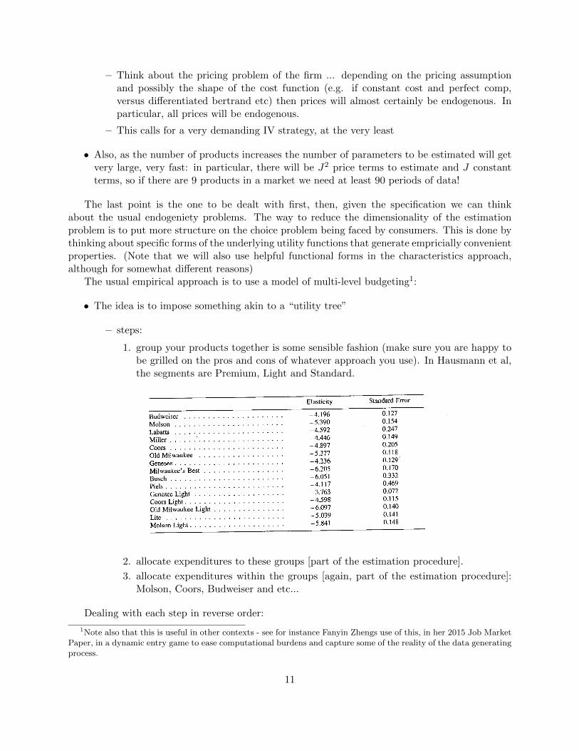
Steps

1. Calculate expenditure share wi of each good i using prices pi, quantities qi, and total expen-diture x =

∑k pkqk.

2. Compute Stone price index: logP =∑

k wk log(pk)

3. Run regression (e.g., IV):

wi = αi +∑k

γik log(pk) + βi log(x

P) + ξi (7)

where ξi is the error term.

4. Recover J + 2 parameters (αi, γi1, . . . , γiJ , βi)

4.2 Hausman, Leonard & Zona (1994) on Beer

This is Hausman, Leonard & Zona (1994) Competitive Analysis with Differentiated Products,Annales d’Econ. et Stat.

It is included here as it is one of the classic applications in the context of merger analysis. Ilikely will skip this in class.

Here the authors want to estimate a demand system so as to be able to do merger analysis andalso to discuss how you might test what model of competition best applies. The industry that theyconsider is the American domestic beer industry.

Note, that this is a well known paper due to the types of instruments used to controlfor endogeniety at the individual product level. This is where the phrase ‘Hausmaninstrument’ comes from in the context of demand estimation.

They use a three-stage budgeting approach: the top level captures the demand for the product,the next level the demand for the various groups and the last level the demand for individualproducts with the groups.

The bottom level uses the AIDS specification where spending on brand i in city n at time t isgiven by:

wi,n,t = αin +∑j

γij log (pjnt) + βi log

(yGntPnt

)+ εint

where yGnt is expenditure on segment G. [note the paper makes the point that the exact form ofthe price index is not usually that important for the results]

The next level uses a log-log demand system

log qmnt = βm log yBnt +∑k

δk log (πknt) + αmn + εmnt

where qmnt is the segment quantity purchased, yBnt is total expenditure on beer, π are segmentprice indices and α is a constant. [Does it make sense to switch from revenue shares at the bottomlevel, to quantities at the middle level?] The top level just estimates at similar equation as themiddle level, but looking at the choice to buy beer overall. Again it is a log-log formulation.

log ut = β0 + β1 log yt + β2 log Πt + Ztδ + εt

where ut is overall spending on beer, yt is disposable income and Πt is a Price Index for Beer overall,and Zt are variables controlling for demographics, monthly factors, and minimum age requirements.

Identification of price coefficients:

13

• recall that, as usual, price is likely to be correlated with the unobservable (nothing in thecomplexity that has been introduced gets us away from this problem)

• what instruments are available, especially at the individual brand level?

– The authors propose using the prices in one city to instrument for prices in another.This works under the assumption that the pricing rule looks like:

log(pjnt) = δj log(cjt) + αjn + ωjnt

where pjnt is the price of good j in city n at time t, cjt represents nation-wide product-costs at time t, αjn are city specific shifters which reflect transportation costs or localwage differentials, and ωjnt is a mean zero stochastic disturbance (e.g., local sales pro-motions.

Here they are claiming that city demand shocks ωjnt are uncorrelated. This allows us touse prices in other markets for the same product in the same time period as instruments(if you have a market fixed effect). Often these are referred to as Hausman instruments.This has been criticized for ignoring the phenomena of nation-wide ad campaigns. Still,it is a pretty cool idea and has been used in different ways in several different studies.

• Often people use factor price instruments, such as wages, the price of malt or sugar as variablesthat shift marginal costs (and hence prices), but don’t affect the ξ’s.

• You can also use instruments if there is a large price change in one period for some externalreason (like a strategic shift in all the companies’s pricing decisions). Then the instrument isjust an indicator for the pricing shift having occurred or not.

Substitution Patterns

The AIDS model makes some assumptions about the substitution patterns between products. Youcan’t get rid of estimating J2 coefficients without some assumptions!

• Top level: Coors and another product (chips). If the price of Coors goes up, then the priceindex of beer PB increases.

• Medium level: Coors and Old Style, two beers in separate segements. Increase in the priceof Coors raises πP , which raises the quantity of light beer sold (and hence increases the salesof Old Style in particular).

• Bottom level: Coors and Budweiser, two beers in the same segment. Increase in the price ofCoors affects Budweiser through γc,b.

So the AIDS model restricts subsitution patterns to be the same between two products any twoproducts in different segments. Is this a reasonable assumption?

14

Figure 3: Demand Equations: Middle Level- Segment Choice

Figure 4: Demand Equations: Bottom-Level Brand Choice

15

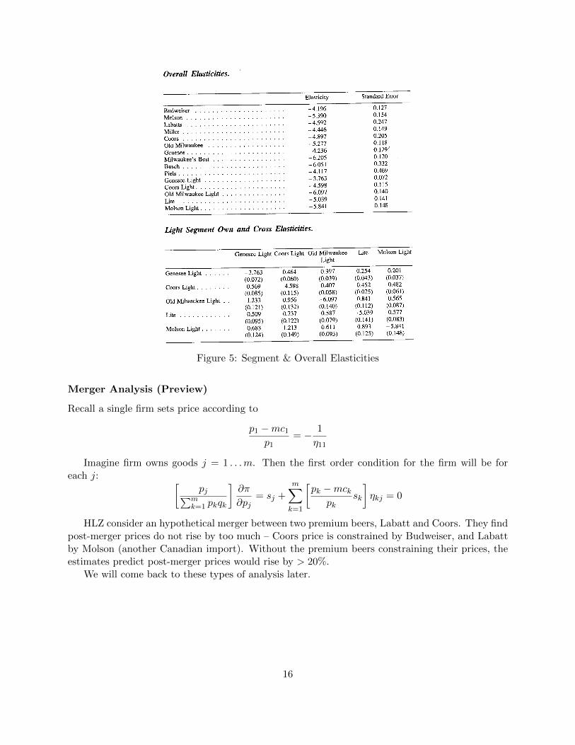
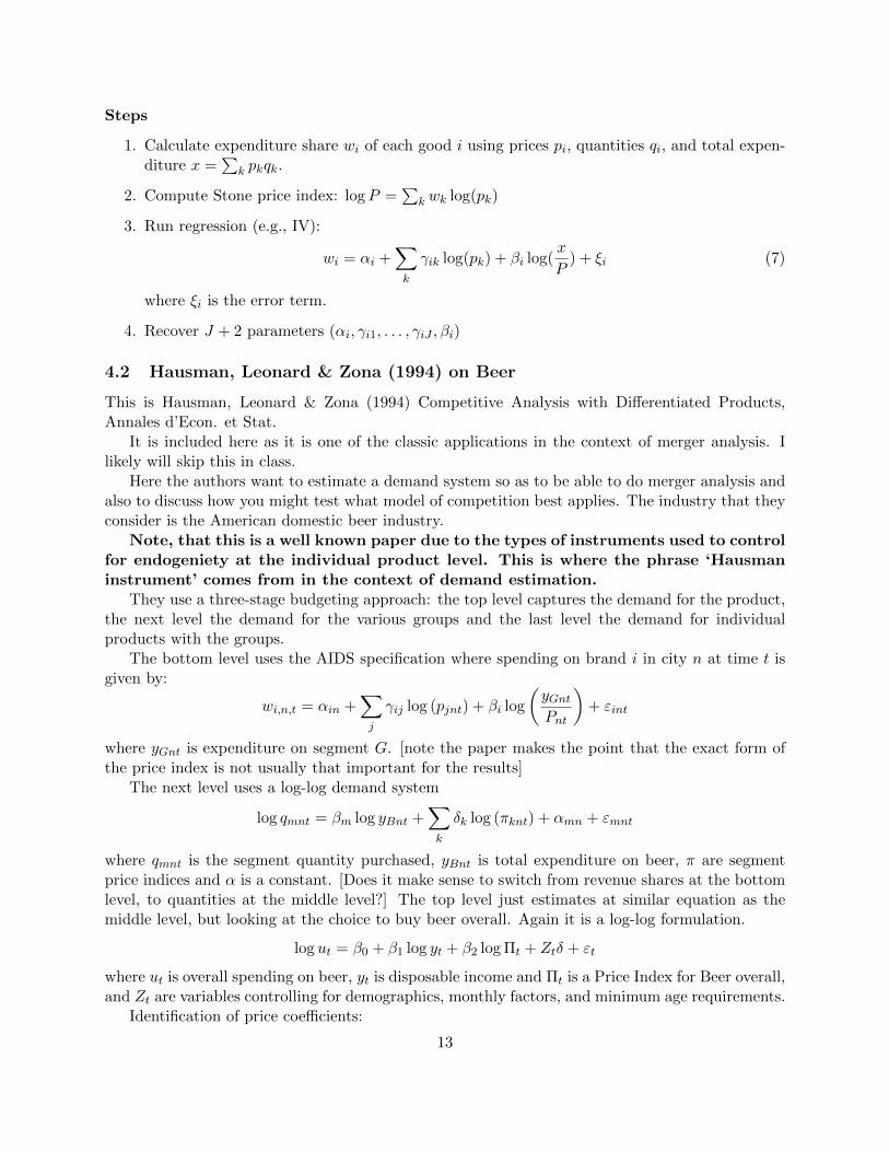
Figure 5: Segment & Overall Elasticities

Merger Analysis (Preview)

Recall a single firm sets price according to

p1 −mc1p1

= − 1

η11

Imagine firm owns goods j = 1 . . .m. Then the first order condition for the firm will be foreach j: [

pj∑mk=1 pkqk

]∂π

∂pj= sj +

m∑k=1

[pk −mck

pksk

]ηkj = 0

HLZ consider an hypothetical merger between two premium beers, Labatt and Coors. They findpost-merger prices do not rise by too much – Coors price is constrained by Budweiser, and Labattby Molson (another Canadian import). Without the premium beers constraining their prices, theestimates predict post-merger prices would rise by > 20%.

We will come back to these types of analysis later.

16

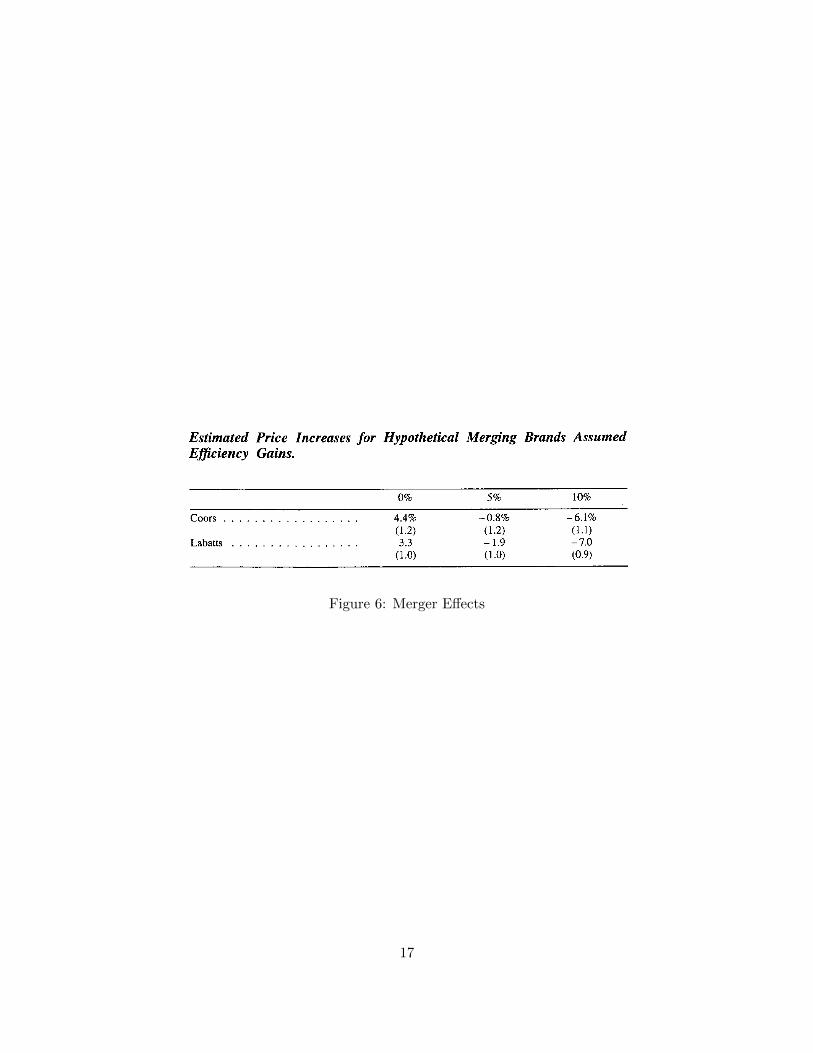
Figure 6: Merger Effects

17

4.3 Chaudhuri, Goldberg and Jia (2006) on Quinolones

Question: The WTO has imposed rules on patent protection (both duration and enforcement) onmember countries. There is a large debate on should we allow foreign multinationals to extent theirdrugs patents in poor countries such as India, which would raise prices considerably.

• Increase in IP rights raises the profits of patented drug firms, giving them greater incentivesto innovate and create new drugs (or formulations such as long shelf life which could be quiteuseful in a country like India).

• Lower consumer surplus dues to generic drugs being taken off the market.

To understand the tradeoff inherent in patent protection, we need to estimate the magnitudeof these two effects. This is what CGJ do.

Market: Indian Market for antibiotics

• Foreign and Domestic, Licensed and Non-Licensed producers.

• Different types of Antibiotics, in particular CGJ look at a particular class: Quinolones.

• Different brands, packages, dosages etc...

• Question: What would prices and quantities look like if there were no unlicensed firms sellingthis product in the market? 2

Data

• The Data come from a market research firm. This is often the case for demand data sincethe firms in this market are willing to pay large amounts of money to track how well they aredoing with respect to their competitors. However, prying data from these guys when theysell it for 10 000 a month to firms in the industry involves a lot of work and emailing.

• Monthly sales data for 4 regions, by product (down to the SKU level) and prices.

• The data come from audits of pharmacies, i.e. people go to a sample of pharmacies andcollect the data.

• Some products have different dosages than others. How does one construct quantity for thismarket?

• Some products enter and exit the sample. How can the AIDS model deal with this?

2One of the reasons I.O. economists use structural models is that there is often no experiment in the data, i.e. acase where some markets have this regulation and others don’t.

18

Estimation and Results

• CGJ estimate the AIDS specification with the aggregation of different brands to productlevel.

Product groups are defined to be indexed by molecule M and domestic/foreign status DF .

Revenue share of each product group i in each region r at time t:

ωirt = αi + αir +∑j

γij ln pjrt + βi ln(XQrt

PQrt) + εirt (8)

where ωirt = xirt/XQrt, prices for each group are aggregated/weighted over individual SKUs,and XQrt is expenditures on quinolones; and price index:

lnPQ = α0 +∑i

αi ln pi +1

2

∑i

∑j

γ̃ij ln pi ln pj (9)

and upper level demand:

ωGrt = αG + αGr +∑H

γGH lnPHrt + βG ln(Xrt

Prt) + εGrt (10)

across different segments H of antibiotics.

• Do not model the choice of individual SKU products:

– Large # of SKUs within each group (dimensionality), lack of price variation at SKUlevel, and varying choice sets over time (entry/exit of SKUs).

– Discrete choice approach difficult due to difficulty mapping revenue shares to physicalshares – dosage of drugs not welll defined.

• Problem for the AIDS model: Over 300 different products, i.e. 90,000 cross product inter-action terms to estimate! CGJ need to do some serious aggregating of products to get ridof this problem: they will aggregate products by therapeutic class into 4 of these, interactedwith the nationality of the producer. I.e., each product will have an own price coefficientγi,i, and a price coefficient for products of different molecules and/or nationalities, denotedγi,10, γi,01, γi,00. (Note that these coefficients are not whether or not the molecule is licensed).Thus, a product i will exhibit the same cross-price elasticity for two different drugs if thosetwo drugs differ in the same way both in molecule and foreign/domestic status. This yields7 product groups (one group is only produced by foreign firms), and 7× 4 price terms.

• Simultaneity bias: SKU revenue share weights (used in computation of price index for eachproduct group) depend on expenditure, and will be correlated with demand shock. Instru-ments: # SKUs within group (violated if # of SKUs affect perceived quality of drug or iscorrelated with advertising), prices at SKU level (due to price controls)

• Supply Side: You can get upper and lower bounds on marginal costs by assuming either thatfirms are perfect competitors within the segment (i.e. p = mc) or by assuming that firmsare operating a cartel which can price at the monopoly level (i.e. p = mc

1+1/ηjj). This is very

smart: you just get a worse case scenario and show that even in the case with the highest

19

possible producer profits, these profits are small compared to the loss in consumer surplus.Often it is better to bound the bias from some estimates rather than attempt to solve theproblem.

• Use estimated demand system to compute the prices of domestic producers of unlicensedproducts that make expenditures on these products 0 (this is what “virtual prices” mean).

• Figure out what producer profits would be in the world without unlicensed firms (just (p−c)qin this setup).

• Compute the change in consumer surplus (think of integrating under the demand curve).

– Product Variety Effect

– Expenditure Switching effect (substitution to other types of antibiotics, not quinolones);holds fixed prices of other products

– Reduced-competition effect: firms adjust prices upwards due to removal of domesticproducts

20

antiinfectives segment ranks second in India,whereas in the world market it is fifth and has ashare of only 9.0 percent. Hence, antiinfectivesare important in India not only from a health

and public policy point of view, but also as asource of firm revenue.

With this in mind, we focus on one partic-ular subsegment of antiinfectives, namely the

TABLE 3—SUMMARY STATISTICS FOR THE QUINOLONES SUBSEGMENT: 1999–2000

North East West South

Annual quinolones expenditure per household (Rs.) 31.25 19.75 27.64 23.59(3.66) (3.67) (4.07) (2.86)

Annual antibiotics expenditure per household (Rs.) 119.88 84.24 110.52 96.24(12.24) (12.24) (9.60) (9.96)

No. of SKUsForeign ciprofloxacin 12.38 11.29 13.08 12.46

(1.50) (1.90) (1.02) (1.06)Foreign norfloxacin 1.83 1.71 2.00 1.58

(0.70) (0.75) (0.88) (0.83)Foreign ofloxacin 3.04 2.96 2.96 3.00

(0.86) (0.86) (0.91) (0.88)Domestic ciprofloxacin 106.21 97.63 103.42 105.50

(5.99) (4.34) (7.22) (4.51)Domestic norfloxacin 38.96 34.96 36.17 39.42

(2.71) (2.68) (2.51) (3.79)Domestic ofloxacin 18.46 16.00 17.25 17.25

(6.80) (6.34) (5.86) (6.35)Domestic sparfloxacin 29.83 28.29 31.21 29.29

(5.57) (6.38) (6.88) (6.57)Price per-unit API* (Rs.)

Foreign ciprofloxacin 9.58 10.90 10.85 10.07(1.28) (0.66) (0.71) (0.58)

Foreign norfloxacin 5.63 5.09 6.05 4.35(0.77) (1.33) (1.39) (1.47)

Foreign ofloxacin 109.46 109.43 108.86 106.12(6.20) (6.64) (7.00) (11.40)

Domestic ciprofloxacin 11.43 10.67 11.31 11.52(0.16) (0.15) (0.17) (0.13)

Domestic norfloxacin 9.51 9.07 8.88 8.73(0.24) (0.35) (0.37) (0.20)

Domestic ofloxacin 91.63 89.64 85.65 93.41(16.15) (15.65) (14.22) (14.07)

Domestic sparfloxacin 79.72 78.49 76.88 80.28(9.76) (10.14) (11.85) (10.37)

Annual sales (Rs. mill)Foreign ciprofloxacin 41.79 24.31 45.20 29.47

(15.34) (8.16) (12.73) (6.48)Foreign norfloxacin 1.28 1.00 0.58 0.73

(1.01) (0.82) (0.44) (0.57)Foreign ofloxacin 54.46 31.84 35.22 31.11

(13.99) (9.33) (9.06) (7.03)Domestic ciprofloxacin 962.29 585.91 678.74 703.81

(106.26) (130.26) (122.26) (87.40)Domestic norfloxacin 222.55 119.71 149.18 158.29

(38.84) (19.45) (26.91) (16.26)Domestic ofloxacin 125.02 96.21 149.36 112.05

(44.34) (30.11) (52.82) (42.59)Domestic sparfloxacin 156.17 121.75 161.30 98.11

(31.41) (25.76) (46.74) (34.20)

Note: Standard deviations in parentheses.* API: Active pharmaceutical ingredient.

1483VOL. 96 NO. 5 CHAUDHURI ET AL.: GLOBAL PATENT PROTECTION IN PHARMACEUTICALS

Figure 7: Summary Statistics

21

not impose it through any of our assumptionsregarding the demand function. The questionthat naturally arises, then, is what might explainthis finding. While we cannot formally addressthis question, anecdotal accounts in various in-dustry studies suggest that the explanation maylie in the differences between domestic andforeign firms in the structure and coverage ofretail distribution networks.

Distribution networks for pharmaceuticals inIndia are typically organized in a hierarchicalfashion. Pharmaceutical companies deal mainlywith carrying and forwarding (C&F) agents, inmany instances regionally based, who each sup-ply a network of stockists (wholesalers). Thesestockists, in turn, deal with the retail pharma-cists through whom retail sales ultimately oc-cur.35 The market share enjoyed by a particularpharmaceutical product therefore depends inpart on the number of retail pharmacists who

stock the product. And it is here that thereappears to be a distinction between domesticfirms and multinational subsidiaries. In particu-lar, the retail reach of domestic firms, as agroup, tends to be much more comprehensivethan that of multinational subsidiaries (IndianCredit Rating Agency (ICRA), 1999).36

There appear to be two reasons for this. Thefirst is that many of the larger Indian firms,because they have a much larger portfolio ofproducts over which to spread the associatedfixed costs, typically have more extensive net-works of medical representatives. The second issimply that there are many more domestic firms(and products) on the market. At the retail level,this would imply that local pharmacists mightbe more likely to stock domestic products con-taining two different molecules, say ciprofloxa-cin and norfloxacin, than they would domesticand foreign versions of the same molecule. Tothe extent that patients (or their doctors) arewilling to substitute across molecules in order tosave on transport or search costs (e.g., going toanother pharmacy to check whether a particular

35 There are estimated to be some 300,000 retail pharma-cists in India. On average, stockists deal with about 75 retailers(ICRA, 1999). There are naturally variations in this structure,and a host of specific exclusive dealing and other arrangementsexists in practice. Pharmaceutical firms also maintain networksof medical representatives whose main function is to marketthe company’s products to doctors who do the actual prescrib-ing of drugs. In some instances, firms do sell directly to thedoctors who then become the “retailer” as far as patients areconcerned, but these are relatively rare.

36 These differences were also highlighted in conversa-tions one of the authors had with CEOs and managingdirectors of several pharmaceutical firms, as part of a sep-arate study.

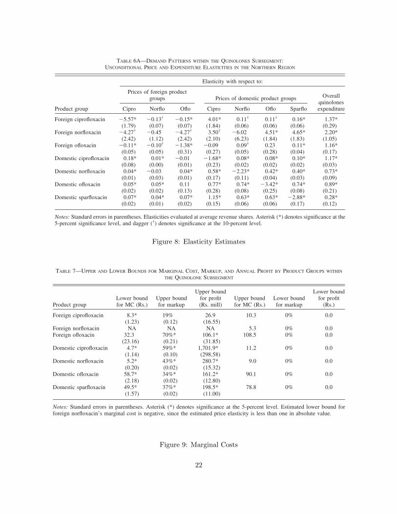
TABLE 6A—DEMAND PATTERNS WITHIN THE QUINOLONES SUBSEGMENT:UNCONDITIONAL PRICE AND EXPENDITURE ELASTICITIES IN THE NORTHERN REGION

Product group

Elasticity with respect to:

Prices of foreign productgroups Prices of domestic product groups Overall

quinolonesexpenditureCipro Norflo Oflo Cipro Norflo Oflo Sparflo

Foreign ciprofloxacin 5.57* 0.13† 0.15* 4.01* 0.11† 0.11† 0.16* 1.37*(1.79) (0.07) (0.07) (1.84) (0.06) (0.06) (0.06) (0.29)

Foreign norfloxacin 4.27† 0.45 4.27† 3.50† 6.02 4.51* 4.65* 2.20*(2.42) (1.12) (2.42) (2.10) (6.23) (1.84) (1.83) (1.05)

Foreign ofloxacin 0.11* 0.10† 1.38* 0.09 0.09† 0.23 0.11* 1.16*(0.05) (0.05) (0.31) (0.27) (0.05) (0.28) (0.04) (0.17)

Domestic ciprofloxacin 0.18* 0.01* 0.01 1.68* 0.08* 0.08* 0.10* 1.17*(0.08) (0.00) (0.01) (0.23) (0.02) (0.02) (0.02) (0.03)

Domestic norfloxacin 0.04* 0.03 0.04* 0.58* 2.23* 0.42* 0.40* 0.73*(0.01) (0.03) (0.01) (0.17) (0.11) (0.04) (0.03) (0.09)

Domestic ofloxacin 0.05* 0.05* 0.11 0.77* 0.74* 3.42* 0.74* 0.89*(0.02) (0.02) (0.13) (0.28) (0.08) (0.25) (0.08) (0.21)

Domestic sparfloxacin 0.07* 0.04* 0.07* 1.15* 0.63* 0.63* 2.88* 0.28*(0.02) (0.01) (0.02) (0.15) (0.06) (0.06) (0.17) (0.12)

Notes: Standard errors in parentheses. Elasticities evaluated at average revenue shares. Asterisk (*) denotes significance at the5-percent significance level, and dagger (†) denotes significance at the 10-percent level.

1498 THE AMERICAN ECONOMIC REVIEW DECEMBER 2006

Figure 8: Elasticity Estimates

foreign product is in stock), in aggregate datawe would expect to find precisely the substitu-tion patterns that we report in Table 6.

Whether the particular explanation we provideabove is the correct one, the high degree of sub-stitutability between domestic product groupsturns out to have important implications for thewelfare calculations. We discuss these in moredetail below when we present the results of thecounterfactual welfare analysis. Another elasticitywith important implications for the counterfactu-als is the price elasticity for the quinolone subseg-ment as a whole, which indicates how likelyconsumers are to switch to other antibioticsgroups, when faced with a price increase for quin-olones. This elasticity is computed on the basis ofthe results in Table A3, and it is at 1.11 (stan-dard error: 0.24); this is large in magnitude,but—as expected—smaller in absolute value thanthe own-price elasticities of the product groupswithin the quinolone subsegment.

The results in Tables 6A and 6B are based onour preferred specification discussed in SectionII. In Tables A4 to A6 in the Appendix, weexperiment with some alternative specifications.Tables A4(a)–A4(c) correspond to a specificationthat includes, in addition to product-group-specificregional fixed effects, product-group-specific (andfor the upper level antibiotics-segment-specific)seasonal effects. We distinguish among three sea-sons—the summer, monsoon, and winter—andreport the unconditional demand elasticities for

the northern region for each of these seasons. Asevident from the tables in the Appendix, our elas-ticity estimates are robust to the inclusion of sea-sonal effects. The demand elasticities in Table A5are based on estimation of the demand system byOLS. Compared to the elasticities obtained by IV,the OLS elasticities are smaller in absolute value,implying that welfare calculations based on theOLS estimates would produce larger welfare lossestimates. Nevertheless, some of the patterns re-garding the cross-price elasticities discussed ear-lier are also evident in the OLS results; inparticular, the cross-price elasticities between dif-ferent domestic product groups are all positive,large, and significant, and in most instances largerthan the cross-price elasticities between drugs thatcontain the same molecule but are produced byfirms of different domestic/foreign status. Theclose substitutability of domestic products indi-cated by both the OLS and IV estimates seems tobe one of the most robust findings of the paper.

B. Cost and Markup Estimates

Table 7 displays the marginal costs, markups,and profits implied by the price elasticity esti-mates of Tables 6A and 6B for each of the sevenproduct groups. Given that our regional effectsimply different price elasticities for each region,our marginal cost and markup estimates alsodiffer by region. Given, however, that based on

TABLE 7—UPPER AND LOWER BOUNDS FOR MARGINAL COST, MARKUP, AND ANNUAL PROFIT BY PRODUCT GROUPS WITHIN

THE QUINOLONE SUBSEGMENT

Product groupLower boundfor MC (Rs.)

Upper boundfor markup

Upper boundfor profit(Rs. mill)

Upper boundfor MC (Rs.)

Lower boundfor markup

Lower boundfor profit

(Rs.)

Foreign ciprofloxacin 8.3* 19% 26.9 10.3 0% 0.0(1.23) (0.12) (16.55)

Foreign norfloxacin NA NA NA 5.3 0% 0.0Foreign ofloxacin 32.3 70%* 106.1* 108.5 0% 0.0

(23.16) (0.21) (31.85)Domestic ciprofloxacin 4.7* 59%* 1,701.9* 11.2 0% 0.0

(1.14) (0.10) (298.58)Domestic norfloxacin 5.2* 43%* 280.7* 9.0 0% 0.0

(0.20) (0.02) (15.32)Domestic ofloxacin 58.7* 34%* 161.2* 90.1 0% 0.0

(2.18) (0.02) (12.80)Domestic sparfloxacin 49.5* 37%* 198.5* 78.8 0% 0.0

(1.57) (0.02) (11.00)

Notes: Standard errors in parentheses. Asterisk (*) denotes significance at the 5-percent level. Estimated lower bound forforeign norfloxacin’s marginal cost is negative, since the estimated price elasticity is less than one in absolute value.

1500 THE AMERICAN ECONOMIC REVIEW DECEMBER 2006

Figure 9: Marginal Costs

22

Figure 10: Counterfactuals

23