Embed Size (px)
Citation preview

i
DEMAND SYSTEM ANALYSIS WITH EMPHASIS ON CONTAINER SIZES OF NON-ALCOHOLIC BEVERAGES.
Authors
Matthew C. Stockton University of Idaho AERS Department
Moscow, Idaho 83844-2334 [email protected]
(208) 885-6047
Oral Capps Jr. Texas A&M University
Agricultural Economics Department College, Station, Texas 7784
[email protected] (979) 845-8491
Selected paper for presentation at the American Agricultural Economics Association Annual Meeting, Providence, Rhode Island, July 24-27, 2005
Copyright 2005 by [Matthew C. Stockton and Oral Capps Jr.]. All rights reserved. Readers may make verbatim copies of this document for non-commercial purposes by any means, provided that this copyright
notice appears on all such copies.

ii
Abstract
A demand system that includes five different beverages of various container sizes
was estimated using a Censor Corrected Almost Ideal Demand System (CAIDS).
Resulting elasticities provide information about intra-product relationships (same
product but different sizes), intra-size relationships (different products same container
size), and inter-product relationships (different products and different sizes).

1
DEMAND SYSTEM ANALYSIS WITH EMPHASIS ON CONTAINER SIZES OF NON-ALCOHOLIC BEVERAGES.
Introduction
The past several decades have seen the proliferation of products that potentially
compete with milk as a beverage. This contention is evident from the ever-increasing
number of non-alcoholic beverages. These facts support the need for a more rigorous
and detailed examination of consumer behavior for non-alcoholic beverages.
In all of the literature on milk demand no research study yet has investigated the
effect of container sizes on elasticity estimates for milk or non-alcoholic beverages. To
date most studies on milk and other non-alcoholic beverages aggregate all of the
products included in the demand system into a single container size measure, the gallon.
An exception to note, which uses the half-gallon as the normalized measure, was the
study by Glaser and Thompson. Interestingly Glaser and Thompson use the half-gallon
measure by default, since the primary focus of their work was on organic milk, which
was at the time almost exclusively sold in half-gallons.
A likely reason for the use of demand systems that have a single unit measure
results from extensive application of the LA/AIDS model. The LA/AIDS model is
generally applied with the inclusion of the Stone index to linearize the system of
equations. It has been shown that the Stone index creates a biased estimate of the
parameters when the unit measures of the right-hand side variables in the demand
equations are not in uniform unit measures. (Moschini). Another possible reason is until
recently data of a disaggregate nature has been unavailable.

2
The departure from the single unit measurement demand system is a step away
from the traditional approach, and a step toward isolating the effect characteristics have
on consumer behavior. Elasticity information by container size, which is hidden in any
aggregated demand model, can be more clearly identified. Capps and Love recognized
this in their 2002 AJAE article on demand analysis when they indicated, “scanner data
from retailers enhances analysts’ ability to understand consumer demand, particularly
food products”. Home Scan Data (HSD) can generally support the construction of these
more sophisticated demand systems.
Package aggregation hides differences in the qualities or characteristics that
makeup the aggregated commodity. For example in a data such as ACNielsen survey
data, milk is bought in various container sizes, but ignoring that by aggregating all
purchases as if they were only one quantity size, implies that the price relationships
estimated from such an aggregation is the result of some kind of weighted relationship
among those container sizes. The problem is not that the estimated coefficients and
resulting elasticities are weighted, but rather there is no way to disentangle the value of
the weights that makeup these estimates of the aggregated demand system. Therefore,
there is no way to measure the effect that a single characteristic, such as container size,
has on consumer price and quantity response. It is, however, the relationships of the
disaggregated products that tell the more complete story. Price relationships, which take
into account container size, would provide valuable decision-making information and a
clearer vision of how the non-alcoholic beverage market functions for at-home

3
consumption. This information could prove invaluable to stakeholders in the milk and
non-alcoholic beverage arena.
In capturing the price effects by container size in a demand system, a much more
detailed understanding of the interrelationships between milk and other non-alcoholic
beverages are possible. Beverages included in this work are of the ready to serve type
and are commonly found in the demand literature as well as on the supermarket shelf.
Carbonated soft drinks (CSDs) are included in most studies about non-alcoholic
beverages, which is no surprise since they have been on an increasing trend for the last
couple of decades and are the most commonly bought non-alcoholic beverage.
According to Nyman and Capps the estimated per capita consumption of CSDs
in 1998 was in excess of fifty gallons annually. Bottled water, and juices also have been
on the increase and compete for a place in the bundle the consumer purchases. In this
study a demand system with these three beverages as well as fluid milk in varying
containers sizes was considered. The inclusion of different container sizes makes this
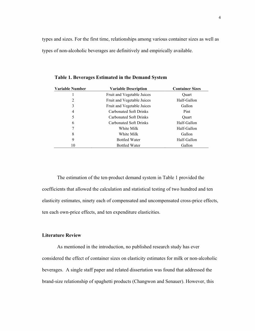
beverage research unique when compared to previously published research. Table 1
provides a complete list of the beverage products and the container size groupings
applied in the demand system.
The demand system will provide several types of price information, including
own-price, cross-price and expenditure elasticities. When these common measures of
price effects are considered in the context of container size, i.e., cross-price elasticities,
they represent the substitutability or complementary nature of beverages of different
4
types and sizes. For the first time, relationships among various container sizes as well as
types of non-alcoholic beverages are definitively and empirically available.
The estimation of the ten-product demand system in Table 1 provided the
coefficients that allowed the calculation and statistical testing of two hundred and ten
elasticity estimates, ninety each of compensated and uncompensated cross-price effects,
ten each own-price effects, and ten expenditure elasticities.
Literature Review
As mentioned in the introduction, no published research study has ever
considered the effect of container sizes on elasticity estimates for milk or non-alcoholic
beverages. A single staff paper and related dissertation was found that addressed the
brand-size relationship of spaghetti products (Changwon and Senauer). However, this
Table 1. Beverages Estimated in the Demand System Variable Number Variable Description Container Sizes
1 Fruit and Vegetable Juices Quart 2 Fruit and Vegetable Juices Half-Gallon 3 Fruit and Vegetable Juices Gallon 4 Carbonated Soft Drinks Pint 5 Carbonated Soft Drinks Quart 6 Carbonated Soft Drinks Half-Gallon 7 White Milk Half-Gallon 8 White Milk Gallon 9 Bottled Water Half-Gallon
10 Bottled Water Gallon

5
demand system used a logit-type demand system, designed to estimate the probabilities
associated with consumer choices. This logit model focused on the brand-size effect in
relation to advertising. Therefore only elasticities associated with advertising were
estimated, not the typical own-price and cross-price elasticities.
Many studies have investigated milk demand but one of the first to estimate a
demand structure for fluid milk products was Rojko. In his 1957 work Rojko used time
series data to estimates single-equation demand models for fluid milk, cream, butter, and
other manufactured dairy products.
Since this first study by Rojko, many different types of studies have been
undertaken using different types of data, as can be seen in Capps’ literature review done
in 2003. A classic example of using disappearance data was that of the 1990 milk
demand study by Gould, Cox, and Perali. Gould, Cox, and Perali applied the LA/AIDS
model and investigated demographic changes over time and their effect on demand for
whole and low-fat milk.
Much of the more current demand work applies a demand systems approach with
some type of survey or scanner data. Of the many different papers published, two are
representative of the issues that arise when estimating a demand system using these
types of data.
Schmit, Chung, Dong, Kaiser, and Gould used a Heckman two-step procedure to
perform single-equation estimates on household scanner data (HSD). One of the major
purposes of using the Heckman procedure is to accommodate censoring. Glaser and
Thompson used a series of four LA/AIDS models on half-gallon sizes of three different

6
milk types, organic, branded white milk, and private label white milk. Each one of the
four models was reflective of a specific fat level. The fat levels used were whole milk,
two percent fat milk, one percent fat milk, and non-fat milk. Although the reader is
intrigued by their comments on the importance of different container sizes, they
nonetheless use only the half-gallon size in their models.
The demand system used in this work includes many of the missing elements not
included in previous research. First and foremost, this work uses a systems approach to
address the price effects of the two most common container sizes of milk as well as the
leading competing products in like sizes. Second, a methodology was used that accounts
for censoring. The methodology proposed by Shonkwiler and Yen was applied. The
Shonkwiler and Yen methodology uses a consistent two-step estimation procedure
referred to as CTS. Much like the single-equation case and the method posed by Heien
and Wessels (HW) the first stage requires a probit estimation. However, it is the second
stage where the CTS diverge from the HW estimation procedure. There are several other
methods of accounting for censoring in a demand system found in the literature, but
many of these require the use of integrals, which may make the estimation of a model
this size intractable (Yen et al. 2003). And thirdly several variations of the Almost Ideal
Demand System (AIDS) from Deaton and Muelbauer, including the AIDS itself and the
Linear Approximation to the AIDS model (LA/AIDS). The advantage to the more
complex AIDS verses the LA/AIDS is that it accounts for unit measure differences
between estimated commodities in the system (Moschini). The AIDS model also is
more appropriate from an aggregation prospective.

7
Data Description
Scanner data have been available from grocery stores since the mid 1970’s. The
first published academic research to appear using store-collected scanner data appeared
in 1987. Scanner data has many different forms. The two primary suppliers in U.S. for
scanner data are, aside from proprietary sources, Information Resources Incorporated
(IRI) and ACNielsen (Bucklin and Gupta). Scanner data have several different forms.
Daily information, as used by Kinoshita et al., in their study of the Japanese milk market,
is not often used. Weekly scanner data, the most commonly used frequency, is generally
a time-series data set (Bucklin and Gupta). The home scan type of data, which is a
survey of household purchases for a specified period, generally a year, is another type of
scanner data, although found less frequently in the literature. The type of data used in
this work is of the home scan type as collected by ACNielsen.
The 1999 ACNielsen home scan data (HSD) are unique in that this data set is
similar to a survey. Each panelist was supplied with a scanner device that he/she used at
home to record grocery items purchased at any grocery store, or other type of store
throughout a given time period. Each panelist represents a unique household, with each
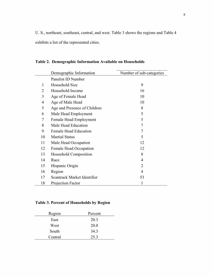
household having eighteen known demographic characteristics. A complete list of the
demographics variables can be reviewed in Table 2.
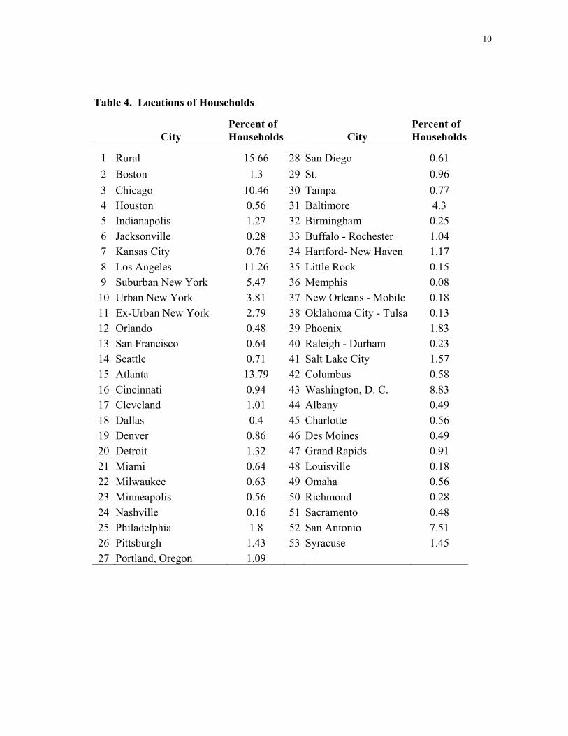
The households are representative of 52 different cities (84.34%) and
unidentified rural areas (15.66%) spread over four regions of the lower 48 states of the
8
U. S., northeast, southeast, central, and west. Table 3 shows the regions and Table 4
exhibits a list of the represented cities.
Table 2. Demographic Information Available on Households Demographic Information Number of sub-categories Panelist ID Number
1 Household Size 9 2 Household Income 16 3 Age of Female Head 10 4 Age of Male Head 10 5 Age and Presence of Children 8 6 Male Head Employment 5 7 Female Head Employment 5 8 Male Head Education 7 9 Female Head Education 7 10 Martial Status 5 11 Male Head Occupation 12 12 Female Head Occupation 12 13 Household Composition 8 14 Race 4 15 Hispanic Origin 2 16 Region 4 17 Scantrack Market Identifier 53 18 Projection Factor 1
Table 3. Percent of Households by Region
Region Percent East 20.3 West 20.0 South 34.3
Central 25.3

9
The scanner information was collected by date of purchase and included only
those panelist that purchased some kind of grocery product in ten out of the twelve-
month periods, making a total of 7,195 participating households. The overall data set
was divided into four product groupings,
(1) Dry grocery (4,111,719 records),
(2) Dairy (873,899 records),
(3) Frozen (1,002,851 records), and
(4) Random weights (507,306 records),
with each grouping having numerous product modules. Each product module was
further subdivided into, brand, size, flavor, form, formula, container, style, type and
variety with each one represented each by a unique UPC number.
For example, in a sub-group such as dairy a product module is Cheese – Natural
– American Cheddar, module number 3550. An overall summary of the number of
modules in each product grouping is given in Table 5.
In addition to demographic information total expenditure and quantity
information were also recorded for each transaction. This information enabled the
imputation of price per unit by transaction, depending on the specified units.
10
Table 4. Locations of Households
City Percent of Households City
Percent of Households
1 Rural 15.66 28 San Diego 0.61 2 Boston 1.3 29 St. 0.96 3 Chicago 10.46 30 Tampa 0.77 4 Houston 0.56 31 Baltimore 4.3 5 Indianapolis 1.27 32 Birmingham 0.25 6 Jacksonville 0.28 33 Buffalo - Rochester 1.04 7 Kansas City 0.76 34 Hartford- New Haven 1.17 8 Los Angeles 11.26 35 Little Rock 0.15 9 Suburban New York 5.47 36 Memphis 0.08 10 Urban New York 3.81 37 New Orleans - Mobile 0.18 11 Ex-Urban New York 2.79 38 Oklahoma City - Tulsa 0.13 12 Orlando 0.48 39 Phoenix 1.83 13 San Francisco 0.64 40 Raleigh - Durham 0.23 14 Seattle 0.71 41 Salt Lake City 1.57 15 Atlanta 13.79 42 Columbus 0.58 16 Cincinnati 0.94 43 Washington, D. C. 8.83 17 Cleveland 1.01 44 Albany 0.49 18 Dallas 0.4 45 Charlotte 0.56 19 Denver 0.86 46 Des Moines 0.49 20 Detroit 1.32 47 Grand Rapids 0.91 21 Miami 0.64 48 Louisville 0.18 22 Milwaukee 0.63 49 Omaha 0.56 23 Minneapolis 0.56 50 Richmond 0.28 24 Nashville 0.16 51 Sacramento 0.48 25 Philadelphia 1.8 52 San Antonio 7.51 26 Pittsburgh 1.43 53 Syracuse 1.45 27 Portland, Oregon 1.09

11
Table 5. Modules Per Grouping Product Grouping Number of Modules Dry Grocery 417 Dairy 43 Frozen 43 Random Weights 119
Data Selection Process
The data selection process includes all of the steps that are necessary to clean and
organize the data in such away so that it was usable for the analytical and descriptive
purpose of this study.
The first step in the process of obtaining a usable data set was to determine which
modules were needed to construct the appropriate data set to be used in the analysis. Of
the many hundreds of modules, modules from two of the groupings were selected and
used in the modeling procedures. Nineteen modules from the dry grocery grouping, and
one from the dairy grouping were included. A complete listing of each individual
module and its grouping can be seen in Table 6. These raw data were extracted from the
original groupings, along with all the appropriate demographic information using SAS.
It should be noted that there were other modules that contained juices, however
these were not in the ready to serve form, i.e. frozen juice concentrates or powdered
drink mixes and were therefore not used.

12
Table 6. Modules Used To Create Data Sets
Sub-Group / Grouping Module Number Product Name
Dry Grocery 1030 Fruit Drinks/Cranberry Dry Grocery 1031 Cider Dry Grocery 1032 Grapefruit Juice Dry Grocery 1033 Apple Juice Dry Grocery 1034 Grape Juice Dry Grocery 1035 Grapefruit Juice - Canned Dry Grocery 1036 Orange Juice - Canned Dry Grocery 1037 Lemon/Lime Juice Dry Grocery 1038 Pineapple Juice Dry Grocery 1039 Prune Juice Dry Grocery 1040 Orange Juice Dry Grocery 1041 Fruit Drinks - Canned Dry Grocery 1042 Fruit Drinks Dry Grocery 1044 Fruit Drinks Remaining Dry Grocery 1045 Fruit Juice Nectars Dry Grocery 1054 Vegetable Juice - Tomato Dry Grocery 1484 Soft Drinks - Carbonated Dry Grocery 1487 Water - Bottled Dry Grocery 1553 Soft Drinks - Low Calorie Dairy Food 3625 White Milk
To transform the data into the appropriate form required several steps. The first
step required identifying the appropriate modules that contain the needed beverage
information. The second step was to extract the appropriate container size, price and
quantity information from the selected modules. The third and fourth steps included
consolidating the data into an annual cross section of households and checking for and
removing any anomalies.

13
The raw data set has two sub-groupings that contain modules of ready to serve
non-alcoholic beverages. The dry grocery sub-group contains modules for juices of all
kinds, CSDs, and bottled water. The dairy sub-group had only the single module, white
milk.
Each of the single modules contains many different types of information about its
general product area. An example will help to clarify what is meant by module
information. The module for white milk, #3625, has information on the characteristics of
the various ways white milk was sold, such as container size and type, brand name, and
fat type. The module also contains purchase information, such as household
identification number, quantity of purchase, and expenditure and coupon or special
purchase information.
For example, milk comes in gallon, half-gallon, quart, pint and half pint sizes,
with a container that may be categorized as plastic, cardboard, pouch or glass.
Additionally, the milk type is a designation of fat content and possibly origin such as
soymilk, goat’s milk, raw milk, as well as other types. The purchase information is based
on transactions where homogeneous items purchased during a single trip to the store are
recorded in number and total expenditure as a group.
Eighteen modules were combined to make the aggregated group called juice,
while the CSD group was comprised of two modules. The bottled water, and white milk,
modules were both single modules. A list of the modules used to create the four-
aggregated beverage groups are summarized in Table 7. Once the aggregations were

14
decided upon, the next phase was to decide on appropriate container size assignments
within each aggregate grouping.
Two of the four aggregate groups, juice, and white milk were sold primarily in
the container sizes of gallons, half-gallons, and quarts. CSDs and water follow a slightly
different pattern that includes both the English and metric systems of volume
measurement. However, for uniformity all four groups which were measured in ounces,
were all converted to the closest container size of pint, quart, half-gallon, or gallon.
Juices were divided into three container size groups, quart, half-gallon and
gallon. Juice sold in containers holding between 16 ounces and 33.8 ounces were classed
as quart size. Juice containers larger than 33.8 ounces and less than or equal to 67.6
ounces were classified as half-gallons. Any juice containers sold that were larger than
67.6 ounces were classified as gallons.
CSDs were grouped into the three sizes of pints, quarts and half-gallons. CSD
containers 16 ounces or less are grouped as pints, while those containers holding more
then 16 ounces and less than 57 ounces were grouped as quarts, and those greater than
57 ounces are classified as half-gallons.

15
For bottled water, an appropriate grouping scheme was difficult to decide on
since to there was no clear uniformity of container size when compared to the other
aggregate groups. Additionally to divide the bottled water into more than two smaller
groups would cause the budget shares to become very small and possibly create
econometric difficulties. From the data it was evident that larger size containers, such as
gallons, are really inexpensive, even less than that of the single liter size. However the
Table 7. List of Used Modules and Assigned Aggregation Groups
Sub-Group Module # Description Title Aggregate Group
Dry Grocery 1030 Fruit Drinks/Cranberry Fruit Juice / FJ
Dry Grocery 1031 Cider Fruit Juice / FJ
Dry Grocery 1032 Grapefruit Juice Fruit Juice / FJ
Dry Grocery 1033 Apple Juice Fruit Juice / FJ
Dry Grocery 1034 Grape Juice Fruit Juice / FJ
Dry Grocery 1035 Grapefruit Juice - Canned Fruit Juice / FJ
Dry Grocery 1036 Orange Juice - Canned Fruit Juice / FJ
Dry Grocery 1037 Lemon/Lime Juice Fruit Juice / FJ
Dry Grocery 1038 Pineapple Juice Fruit Juice / FJ
Dry Grocery 1039 Prune Juice Fruit Juice / FJ
Dry Grocery 1040 Orange Juice Fruit Juice / FJ
Dry Grocery 1041 Fruit Drinks - Canned Fruit Juice / FJ
Dry Grocery 1042 Fruit Drinks Fruit Juice / FJ
Dry Grocery 1044 Fruit Drinks Remaining Fruit Juice / FJ
Dry Grocery 1045 Fruit Juice Nectars Fruit Juice / FJ
Dry Grocery 1054 Vegetable Juice - Tomato Fruit Juice / FJ
Dry Grocery 1055 Vegetable Juice Remaining Fruit Juice / FJ
Dry Grocery 1484 Soft Drinks - Carbonated Carbonated Soft Drinks / CSD
Dry Grocery 1487 Water - Bottled Bottled Water / BW
Dry Grocery 1553 Soft Drinks - Low Calorie Carbonated Soft Drinks / CSD
Dairy Food 3625 White Milk White Milk / WM

16
larger container size is not convenient for carrying around, while the smaller containers
are more expensive but are easily toted. Therefore two groupings were made, one of
containers smaller than 67.6 ounces, and another of containers holding more than 67.6
ounces. The smaller container sizes were converted to half-gallon equivalents, while the
larger sizes were converted to the gallon-size equivalents.
White milk was subdivided into two groups, with gallons being the most
purchased size followed by half-gallons. The half-gallon size ranged from 33.9 to 101.4
ounces and the gallon size being any container greater than 101.4 ounces. Quarts were
not used since there were some anomalies associated with the data.
Once the modules were extracted from the raw data, aggregated and subdivided
into one of the ten products, several things needed to be done to create the appropriate
cross-sectional data set. Demographic information was necessary to accommodate the
imputation of missing prices and for the estimation of the cumulative distribution
function (cdf) and probability density function (pdf) variables needed for the estimation
of the censored model.
The HSD data is collected in the form of transactions. Each observation was date
specific, with purchase and product characteristic information. The purchase information
was shown as a total expenditure amount for the transaction. This expenditure was
identified as “price paid deal” or “price paid non-deal” where the total actually spent by
the household was the price paid non-deal if no promotion or coupon was present, or
price paid deal minus coupon value in the event of a discount. The price paid for each
item was the total expenditure for the transaction divided by the quantity bought in that

17
transaction. For the purposes of this work, a transaction is defined as the purchase of a
single product type in a single time period. A transaction may be for only one item such
as a single gallon of milk or for many items such as the purchase of twenty-four, 12-
ounce cans of a single type of CSD.
To create the annual cross-sectional data set to be used in this analysis an average
price per household was calculated for each of the ten products. Tables 8 and 9 lists the
descriptive price and quantity statistics from the final data set. The descriptive statistics
are only for those households who purchased a positive quantity during the year of 1999.
Included statistics are average price and quantity, standard deviations, minimum and
maximum prices and quantities.
Table 8. Price Statistics for Households That Purchased the Ten Beverages
Beverage Type Container
Size
Number of Households
That Purchased
Average Price
Standard Deviation
Minimum Price
Maximum Price
Fruit Juice Quart 6,058 1.58 0.89 0.00 7.84 Fruit Juice Half-Gallon 6,789 2.07 0.60 0.00 6.79 Fruit Juice Gallon 3,952 3.36 1.41 0.00 9.72
Bottled Water Half-Gallon 3,847 1.51 0.74 0.00 5.68 Bottled Water Gallon 3,056 0.78 0.23 0.00 2.59
CSD’s* Pint 6,573 0.34 0.14 0.00 1.67 CSD’s Quart 4,807 0.93 0.37 0.00 3.87 CSD’s Half-Gallon 6,770 1.93 0.58 0.00 4.07
White Milk Half-Gallon 5,428 1.66 0.41 0.00 3.95 White Milk Gallon 5,404 2.52 0.38 0.00 5.73
* CSD’s is an acronym for Carbonated Soft Drinks
The average price was calculated by dividing the total annual expenditure for
each product by household, by the total annual quantity bought of that product by that

18
household. This price and quantity information was retained for each of the ten products
for each household. In the event that a household did not purchase any of a particular
product the price was unrecorded. Some households purchased product for a zero price.
Table 9. Quantity Statistics for Households That Purchased the Ten Beverages
Beverage Type Container
Size
Number of Households
That Purchased
Average Number of
Units Purchased
Standard Deviation
Minimum Number of
Units Purchased
Maximum Number of
Units Purchased
Fruit Juice Quart 6,058 22.16 33.44 0.08 558.30Fruit Juice Half-Gallon 6,789 25.99 29.85 0.69 324.70Fruit Juice Gallon 3,952 7.36 11.13 0.75 225.96
Bottled Water Half-Gallon 3,847 10.02 21.98 0.13 452.05Bottled Water Gallon 3,056 16.75 36.76 1.00 430.00
CSD’s* Pint 6,573 273.99 408.70 0.75 17,613.00CSD’s Quart 4,807 26.63 67.11 0.63 1,082.80CSD’s Half-Gallon 6,770 31.70 35.93 0.93 455.92
White Milk Half-Gallon 5,428 16.24 24.03 0.89 597.00White Milk Gallon 5,404 34.11 36.71 1.00 376.00
*CSD’s an acronym for Carbonated Soft Drinks.
The annual expenditure sum for each product by household was retained so that
gross expenditures could be calculated as well as budget shares for each product. The
final average budget shares range from just over 23% for CSD pints to less than 2% for
bottled water in the gallon size. Table 10 shows all of the budget shares.
Prior to calculating the average annual price and quantities, several things were
done to reduce anomalies in the final data set. By using Chebychev’s inequality, any
transactional prices greater than five standard deviations from the mean price of that
product were dropped from the data set. From Table 11 it can be seen that of the more

19
than six hundred thousand transactions less than two tenths of a percent were dropped.
The Chebychev’s inequality was performed prior to aggregation across households.
*CSD’s an acronym for Carbonated Soft Drinks
Table 10. Average Budget Shares by Type and Container Size
Beverage Type Container Size Average Budget Share Fruit Juice Quart 6.9% Fruit Juice Half-Gallon 15.1% Fruit Juice Gallon 4.0% Fruit Juices All 26.0%
Bottled Water Half-Gallon 2.0% Bottled Water Gallon 1.6% Bottled Water All 3.6%
CSD’s* Pint 23.8% CSD’s Quart 3.9% CSD’s Half-Gallon 17.1% CSD’s All 44.9%
White Milk Half-Gallon 6.2% White Milk Gallon 19.7% White Milk All 25.5%
Table 11. Effect of Using Chebychev's Inequality with Five Standard Deviations
Product
# Of Observations
Without Chebychev's
# Of Observations
With Chebychev's
Number of lost Observations
Percent of Lost Observations
Fruit Juices Quarts 5,596 5,580 16 0.29%
Fruit Juices Half-Gallons 4,720 4,720 0 0.00%
Fruit Juices Gallons 147,388 147,388 0 0.00%
Bottled Water Half-Gallon 75,669 75,669 0 0.00%
Bottled Water Gallon 21,369 21,369 0 0.00%
Carbonated Soft Drinks Pints 142,904 142,258 646 0.45%
Carbonated Soft Drinks Quarts 48,887 48,873 14 0.03% Carbonated Soft Drinks Half-Gallons 144,574 144,309 265 0.18%
White Milk Half-Gallons 18,719 18,655 64 0.34%
White Milk Gallons 25,832 25,832 0 0.00% Totals 635,658 634,653 1,005 0.16%

20
The next step in obtaining the usable data set was to add demographic
information. The HSD data set has a demographic sub file with 18 different
demographic categories. The eighteen categories are described in chapter two. All of the
demographic information was added for each of the 7,195 households. By aggregating
the data across households a cross sectional data set was created. In 170 cases household
consumed none of the ten products during the year. These 170 households were
excluded from the study. Even among the reaming 7,025 households not all bought all
ten products sometime during the year, and where no purchases were made, no observed
price was recorded or budget share allotted to the purchase of that product. In order for
the data set to be used appropriately in a demand system it was necessary to fill in these
unobserved prices. This was accomplished through a first order imputation process. A
full discussion of the methods and information used in these imputations is discussed in
the methodology portion of this chapter.
Methodology
Price Imputations
In order to estimate the demand system each of the households must have price
information for each product. Since many of the households only purchased some of the
products, prices for non-purchased products were not recoverable. By using the
demographic variables a simple OLS regression was used to impute those missing
prices.

21
An OLS regression was performed for each of the ten products using only those
observations where price for the chosen product were observed. Figure 1 shows
equation 5-1, the mathematical representation of the OLS regression equations and the
explanation of the variables used for the price imputation. A summary of the outcome of
the OLS coefficient estimates with standard errors, t-statistics and p-values can be gotton
from the authors.
(5-1)
hhih
hihhihhihhihhihhih
hihhihhihhihhihhih
h ihhihhihhihhihih
i*NMβ
*Rβ*Rβ*Rβ*Sβ*Jβ*Jβ
*Rβ*Eβ*Eβ*Cβ*Aβ*Aβ
A*β*Hβ*Hβ*Hβ*IββPi
ε++
++++++
++++++
+++++=
18
31721611514213112
112101983726
1534231210
ˆ
ˆˆˆˆˆˆ
ˆˆˆˆˆˆ
ˆˆˆˆˆˆ
Equation 5-1. The OLS Regression equations used to impute missing prices.
Where i = {1,2,3,,,……10} number of products, and h = {1,2,3,,, ……7190} number of households, observations.
ihP - Where P is the actual price of the ith product and hth household.
i0β̂ - The intercept term for the base profile for the ith product.
ih1β̂ - The effect of household income on the ith product of the hth household.
Ih - The average income of the hth household. ih2β̂ - The effect of having a one person household on the ith product of the hth household
H1h – The indication of household size of one person, for the hth household.
ih3β̂ - The effect of having a two people household on the ith product of the hth household.
H2h – The indication of household size two people, for the hth household.
ih4β̂ - The effect of having a two people household on the ith product of the hth household.
H3h – The indication of household size of three people, for the hth household.
ih5β̂ - The effect of having a female household head less than 25 years old on the ith price of the hth
household. A1h - The indication of a female household head less than 25 years old for the hth household. Figure 1. Mathematical representation of the OLS regression equations

22
ih6β̂ - The effect of having a female household head between than 40 and 64 years old on the ith price the hth household. A2h - The indication of a female household head between 40 and 64 years old for the hth household.
ih7β̂ - The effect of having a female household head 65 years old or older on the ith price of the hth household. A3h - The indication of a female household head 65 years old or older for the hth household.
ih8β̂ - The effect of having no children under 18 years old in the household on the ith price of the hth household. Ch - The indication of having no children under 18 years old in the household for the hth household.
ih9β̂ - The effect of having female household head with a high school education or less on the ith price of the hth household E1h - The indication of having a female household head with a high school education or less for the hth household
ih10β̂ - The effect of having female household head with more than four years of college on the ith price of the hth household. E2h - The indication of having a female household head with more than four years of college for the hth household.
ih11β̂ - The effect of a household with a race other than white on the ith price of the hth household.
Rh - The indication of a household with a race other than white for the hth household.
ih12β̂ - The effect of the female household head having no employment on the ith price of the hth household. J1h - The indication of the female household head having no employment for the hth household.
ihf 13β̂ - The effect of the female household head working less than 30 hours a week on the ith price of the hth household. J2h - The indication of the female household head working less than 30 hours a week for the hth household.
ih14β̂ - The effect of a non-Hispanic household on the ith price of the hth household Sh - The indication of a non-Hispanic household for the hth household.
ih15β̂ - The effect of the household located in the eastern region of th U.S. for the Ith price of the hth
household. R1ih- The indication that the hth household is located in the eastern region of the U.S..
ih16β̂ - The effect of the household located in the western region of th U.S. for the Ith price of the hth
household.
R2ih - The indication that the hth household is located in the western region of the U.S. .
ih17β̂ - The effect of the household living in the central region of th U.S. for the ith price of the hth
household.
R3ih - The indication that the hth household is located in the eastern region of the U.S. .
ih18β̂ - The effect of the household living outside a city for the Ith price of the hth household.
Figure 1. Continued.

23
NMh – The indication of the hth households living outside a city.
εih – The unexplained error for the ith price of the hth household. Figure 1. Continued.
All of the demographic variables in the regression model except household
income were indicator variables. The estimated intercept term corresponds to the base
demographic profile. In this case the base profile is that of a white Hispanic household
with children under eighteen years of age, with a household size of more than four
people, having a female head of house that has some college education, between the ages
of twenty-five and forty, works more than 30 hours a week, and lives in the southern
region of the U.S. in a city. Imputation for each price was made using the estimates from
the regressions of only those households that purchased that product. The predicted
prices were then imputed using the estimated coefficients. The predicted prices were
used to fill in any missing prices.
Model Selection
Two models were likely candidates to estimate the elasticities the Almost Ideal
Demand System (AIDS) model and the Linear Approximation of the Almost Ideal
Demand System (LA/AIDS). The AIDS model is deemed to be the more appropriate
model verses the LA/AIDS. Both models are well suited to cross-sectional data, however
as mentioned previously the LA/AIDS model contains the Stone index which has been
shown to result in biased estimates of the parameters (Moschini). However the AIDS
model is a non-linear model and is more complex to apply then LA/AIDS. The AIDS
model has the additional advantage of having desirable properties when aggregating, in

24
this case over consumers. An additional complication is the fact that the data has missing
information and therefore requires some method to account for censored observations.
The Shonkwiler and Yen Consistent Two Step, CTS, procedure was applied.
Although the primary model estimated was the Censored AIDS (CAIDS), the
linerized version the Censored LA/AIDS (CLA/AIDS), was estimated in order to
establish starting values for the non-linear version. Additionally the results from the
linerized version of the model helped to determine the robustness of the resulting
estimates and provided reference information. The CLA/AIDS results were used to
gauge differences in the compensated and uncompensated own-price and cross-price
elasticities as well as expenditure elasticities versus estimating the CAIDS. The
difference between the system estimates can be attributed to approximation errors, errors
due to linearizing, and/or the Stone index bias. In a comparison of the censored verses
non-censored models, complete matrices of elasticities and their associated p-values are
provided. The results of these comparative models are available upon request from the
authors.
Estimation of the Models
The AIDS model as specified by Deaton and Muellbauer is of the PIGLOG class
indicating that price is independent from expenditure in the log form.
(5-2) ihhhijhijiih Pxpj εβγαω +′′−+∑= =+ )ln(*ln13
1 Equation 5-2 General AIDS model specification.
i = 1,2,3,…,10 number of products

25
h = 1,2,3,……7025 number of households, observations
where ωih = the budget share of the ith product of the hth household defined as
(5-3) h
ihihih
xqp *
=ω
Equation 5-3 Budget share equation.
where iα is the constant coefficient in the share equation i, and γij is the slope coefficient
associated with good j in the i share equation .
Total expenditure for the hth household is defined as
(5-4) ∑ ==
13
1iihihh qpx
Equation 5-4 Expenditure equation. Where the LA/AIDS specification of lnP* is defined in equation 5-5a as
(5-5a) ∑ ==′′ 10
1 lnln k khkhh pP ω
Equation 5-5a The Stone approximation.
where pih is the price of good i for the hth household. The lnP*, price index, for the AIDS
specification is defined in equation 5-5b as
(5-5b) jkkjk jk kh ppP lnln21ln 10
1
10
1
10
10 ∑ ∑∑ = == ++=′′ γαα
Equation 5-5b The AIDS and QAIDS expenditure equation. where k is a counter from 1,2,,,…..10.
The uncensored models automatically satisfy the adding-up restriction if the following
conditions hold.
(5-6) ∑==
13
11
iiα ,∑=
=13
10
iijγ , ∑=
=13
10
iiβ

26
Equation 5-6 Conditions to ensure the adding-up restriction hold. The restrictions for maintaining homogeneity are satisfied if and only if, the sum of all
gamma ij’s for each i equal zero.
(5-7) ∑ ==
13
10
jijγ
Equation 5-7. Conditions necessary to ensure that the homogeneity restriction is
maintained.
The symmetry condition is satisfied if and only if that all gamma ij’s equal the gamma
ji’s.
(5-8) γij = γji
Equation 5-8. Conditions to ensure that the symmetry restriction is maintained in the
AIDS and LA/AIDS models.
However, the CTS censoring procedure add additional variables to be estimated and
modifications in the three conditions must be made to impose these classical conditions.
Censored-Correction Conditions
The first stage of the CTS is known as the selection stage, which refers to the
discrete choice where the dependent variable is a qualitative choice variable. In this case,
the choice was to purchase or not to purchase the given product. This choice variable
was assigned a value of (1) for having purchased the product during the year or (0) for
not having purchased the product during the year. The choice variable was then modeled
using a probit. The probit estimation process produces two important factors that
carryover into the second stage of the CTS procedure: (1) the estimated cumulative
distribution function (cdf) and (2) the probability distribution function, (pdf). Both are

27
functions of the demographic variables. These carryover values represent the adjustment
to the demand system necessary to account for the censored observations. With the
imposition of the CTS, the model was then specified as
(5-9) ihihiihhhijhijiih fdpfdcPxpj εϕβγαω ++′′−+∑= =+ ˆ*ˆ*)]ln(*ln[ 13
1
Equation 5-9 Censored AIDS model specification, (CAIDS).
For both model specifications, the CLA/AIDS, and CAIDS, the variables remain
unchanged, as do the conditions for adding-up and homogeneity. However, a special
condition must now be imposed to assure symmetry, to account for the multiplication of
the cdf over each equation. The new condition is
(5-10) cdfi*γij = cdfj*γji which implies ijjh
ihji
cdfcdf γγ *=
Equation 5-10. The conditions to ensure that the symmetry restriction for the censored AIDS model hold.
Estimation of the Probit Model (Selection Stage)
The variables used in the probit model are not the same variables included in the
demand model. The probit model was used to identify choice, and in this case
households have observed prices and have made a choice about consumption. Therefore,
something other than price was used to explain their decision to consume. This
reasoning is consistent with the budgeting process concept. Only demographic variables
were used in this phase of the probit modeling process.
The right hand side (RHS) variables used in the probit model were income,
household size, age, education, employment status of the female head of house, presence
28
of children under eighteen years of age, race, region, and urban or non-urban dweller. In
cases where the household had no female head, the indicators for the male head of house
were used.
All of the RHS variables were indicator variables except income, which though
not technically continuous, was treated as such. The incomes for households were
reported within a range, therefore any given household in a specific range were assigned
the average for that range. Summing the lowest and the highest boundaries of the range
and dividing by two provided the averaged range. It should be noted that incomes less
than $5,000.00 were averaged to $2,500, and for incomes over the $100,000 measure
were set at $100,000.
Household size was classified into four groups: group1, single individual
households (hs1); group 2, households of two individuals (hs2); group3, households with
3 individuals (hs3); and group 4, households with four or more individuals (hs4). Age of
the female head of house was divided into four ranges: range 1, female heads less than
twenty-five years of age (age25); range 2, female heads twenty-four to thirty-nine years
of age (age40); range 3, female heads forty to sixty-five years of age (age50); and range
4, female heads over sixty-five years of age (age65). Households with children present
under the age of eighteen years of age were coded as (child), and those households
without children present under the age of eighteen years of age were coded as (child0).
Female heads of house education level had three groups: group1, female heads with a
high school or less education (edufh); group2, female heads of house with some college
(edufsc); and group3, female heads with at least one degree (edufcp). Employment of the

29
female heads also was separated into three groups: group1, female head not employed
for pay (unemp); group2, female head of house employed but less than thirty-five hours
per week (ptemp); and group3, female heads of house employed thirty-five or more
hours per week (ftemp).
Households across the United States were classed in four general locations:
area1, east; area2, west; area3, central; and area4, south. Households were identified as
within an urban area (metro) or not (nonmetro). The dependent variable was a binary
choice value of the ith product, where a one (1) represents households that bought some
of the ith product, and zero (0) represents households where none of the ith product was
bought, where i = 1,2,3,…10. All of these conditions were imposed on all of the models.
Only nine equations were estimated with the thirteenth being imputed because of the
restrictions imposed on the model. A complete summary of the probit results is available
on request.
The implementation censoring process of the CLA/AIDS and CAIDS are
parallel. The same two-step process was used for both models. The probit for the all four
models was the same estimation of the same variables resulting in one set of cdf’s and
pdf’s for all of the censored models. The cdf and pdf from the probit analysis, stage-one
were saved and used in the next phase. The cdf was multiplied by the specific product i’s
demand equation (equation (5-9)) and the pdf was weighted by a new parameter (φ).
Once the effect of censoring has been accounted for in the estimation process, providing
the conditions of symmetry hold, the standard elasticity formulae for each of the demand
systems may be applied.

30
Elasticity Estimates for the CLA/AIDS , LA/AIDS
The uncompensated elasticity equations for the CLA/AIDS model are the same
as the standard LA/AIDS as taken from Green and Alston version number iii. The εij’s
are the uncompensated own-price and cross-price elasticities.
(5-11) ijiijijij ωωβγδε /)/( −+−=
Equation 5-11. The LA/AIDS model uncompensated elasticities formula. where the Kronecker delta (δ) equal one when i = j.
The compensated elasticity, Eij’, incorporates the Slutsky relationship where the share
weighted income effect was added to the compensated elasticity.
(5-12) ijijij ηωε *' +=Ε
Equation 5-12. The LA/AIDS model compensated elasticities formula.
ηi was the expenditure elasticity of the ith product where
(5-13) )1( iii ωβη +=
Equation 5-13 The LA/AIDS model expenditure elasticities formula.
Elasticity Estimates for the CAIDS and AIDS
Since the AIDS was a non-linear model and the elasticities are defined using
differentiation of the share equations, the AIDS elasticities are different for those of the
LA/AIDS model for both uncompensated and compensated elasticities. However, the
expenditure elasticities for the two models are identical, since the expenditure portions

31
of the two equations are identical. The uncompensated own-price and cross-price
elasticity equations for the CAIDS and AIDS are defined as:
(5-14) iik kjijiijijij ωγβαβγδξ /)( 13
1** ∑ =−−+−=
Equation 5-14. Non-Linear AIDS model uncompensated elasticity formula.
Where the Kronecker delta (δ) equals one when i = j.
The compensated elasticity, ξij’, incorporates the Slutsky relationship where the share
weighted income effect was added to the compensated elasticity.
(5-15) ijiijij Ν+=′ *ωξξ
Equation 5-15. Non-Linear AIDS model uncompensated elasticity formula.
where Ni was the expenditure elasticity of the ith product, where
(5-16) )1( iii ωβ+=Ν
Equation 5-16. Non-Linear AIDS model formula for the expenditure elasticity.
All four models were estimated, CLA/AIDS, LA/AIDS, CAIDS and AIDS. The
only elasticities reported in the main body of this paper are from the CAIDS model the
reaming tables of elasticites are available upon request from the authors. Three different
kinds of elasticities are reported, own-price, cross-price and expenditure elasticities.
Own-price and cross-price elasticities included both compensated and uncompensated.
The parameter estimates with the standard errors and t-statistics for the CAIDS model
are also available from the authors?. The matrices of uncompensated, compensated, and
expenditure elasticities for the CAIDS model are in Tables 13, and 14.

32
Results: CAIDS Estimates
Because of the size of the model and the number of elasticities involved, only the
censored corrected non-linear AIDS compensated elasticities are discussed in the
remaining results. To further facilitate the task of assembling the results in a
comprehensible manner, a series of comparisons were made. The first sets of
comparisons were based on individual product verses all other products which could be
considered an inter-product comparison. The comparisons rank the products and place
them in order of effect, ranging from the largest substitutes to smallest complement. The
effects are either net substitutes or net complements since they are compensated
elasticities. The second sets of comparisons were done by product type, and are referred
to as intra-product comparisons. The third set of comparisons were done by container
size, this grouping was referred to as an intra-size grouping. The Final set of
comparisons were done by comparing categories, such as all white milk with all fruit
juices, this comparison was referred to as an intra-category comparison. In this last
comparison the evaluation was based on significance and sign.
To help facilitate a more concise reporting of the results all references to the
beverages henceforth will be in the form of acronyms. Acronyms for the ten beverage
products will be fruit juices denoted as FJ with sizes of quart, Q, half-gallon, H, and
gallon, G. Bottled water as BW with sizes of half-gallon or less, H, and G, more than a
half-gallon. CSDs are in sizes of pint, P, quart, Q, and half-gallon, H. White milk
denoted as WM with sizes of quart, Q, half-gallon, H, and gallon, G. A reference table is
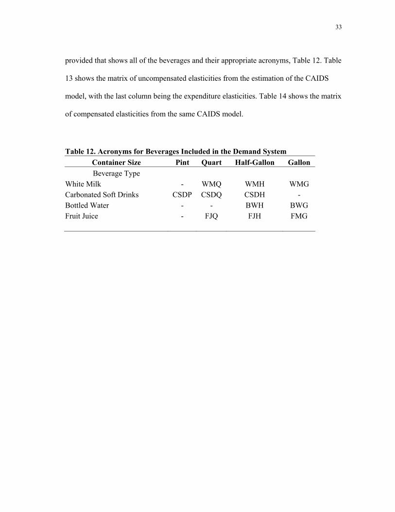
33
provided that shows all of the beverages and their appropriate acronyms, Table 12. Table
13 shows the matrix of uncompensated elasticities from the estimation of the CAIDS
model, with the last column being the expenditure elasticities. Table 14 shows the matrix
of compensated elasticities from the same CAIDS model.
Table 12. Acronyms for Beverages Included in the Demand System Container Size Pint Quart Half-Gallon Gallon Beverage Type
White Milk - WMQ WMH WMG Carbonated Soft Drinks CSDP CSDQ CSDH - Bottled Water - - BWH BWG Fruit Juice - FJQ FJH FMG

34
Table 13. Uncompensated Elasticities of the CAIDS Model Products FJQ FJH FJG CSDP CSDQ CSDH WMH WMG BWH BWG Ni
FJQ -1.5199 -0.0052 0.0471 0.2491 0.0581 -0.0210 0.1415 0.1421 0.0596 0.0042 0.0042
p-value 0.00 0.89 0.08 0.00 0.10 0.51 0.01 0.04 0.03 0.89 0.89
FJH -0.0150 -0.5817 0.0214 -0.0273 -0.0834 -0.0874 -0.0954 -0.1760 0.0344 -0.0197 -0.0197
p-value 0.40 0.00 0.14 0.27 0.00 0.00 0.00 0.00 0.01 0.20 0.20
FJG 0.0322 0.0181 -0.6580 -0.0206 0.0769 -0.4347 -0.3256 -0.0096 0.1216 -0.2767 -0.2767
p-value 0.48 0.74 0.00 0.81 0.24 0.00 0.00 0.94 0.03 0.00 0.00
CSDP 0.0590 -0.0204 0.0111 -1.1392 0.1270 0.0032 0.0342 -0.1548 0.0585 -0.0278 -0.0278
p-value 0.00 0.19 0.45 0.00 0.00 0.81 0.10 0.00 0.00 0.04 0.04
CSDQ 0.1181 -0.2965 0.0811 0.8015 -2.4924 -0.3251 -0.3663 1.0429 0.2543 0.3533 0.3533
p-value 0.05 0.00 0.22 0.00 0.00 0.00 0.00 0.00 0.00 0.00 0.00
CSDH -0.0299 -0.0920 -0.0883 -0.0119 -0.0807 -0.6640 -0.0896 -0.1161 0.0200 0.0190 0.0190
p-value 0.02 0.00 0.00 0.52 0.00 0.00 0.00 0.00 0.03 0.23 0.23
WMH 0.2163 -0.1166 -0.1643 0.3059 -0.2442 -0.0993 -0.1753 0.0531 -0.0379 0.0602 0.0602
p-value 0.00 0.04 0.01 0.00 0.00 0.04 0.22 0.66 0.48 0.35 0.35
WMG 0.0334 -0.1414 0.0172 -0.1906 0.2053 -0.0868 -0.0422 -0.7027 -0.0900 -0.0654 -0.0654
p-value 0.18 0.00 0.50 0.00 0.00 0.00 0.27 0.00 0.00 0.02 0.02
BWH 0.2311 0.3275 0.2827 0.8055 0.4980 0.2660 -0.1554 -0.7787 -2.7807 0.7143 0.7143
p-value 0.02 0.00 0.01 0.00 0.00 0.00 0.35 0.00 0.00 0.00 0.00
BWG -0.0603 -0.2007 -0.5928 -0.4076 0.8250 0.2676 -0.0338 -0.7797 0.8196 -1.1234 -1.1234
p-value 0.63 0.16 0.00 0.04 0.00 0.11 0.89 0.02 0.00 0.01 0.01 * See Table 12 for a complete explanation of the acronyms (Page 33)

35
Table 14. Compensated Elasticities of the CAIDS Model Products FJQ FJH FJG CSDP CSDQ CSDH WMH WMG BWH BWG
FJQ -1.4613 0.1225 0.0807 0.4505 0.0914 0.1232 0.1936 0.3054 0.0762 0.0179
p-value 0.00 0.00 0.00 0.00 0.01 0.00 0.00 0.00 0.01 0.55
FJH 0.0564 -0.4260 0.0624 0.2183 -0.0428 0.0884 -0.0318 0.0232 0.0547 -0.0029
p-value 0.00 0.00 0.00 0.00 0.01 0.00 0.18 0.43 0.00 0.85
FJG 0.1346 0.2414 -0.5993 0.3314 0.1351 -0.1827 -0.2344 0.2759 0.1507 -0.2527
p-value 0.00 0.00 0.00 0.00 0.04 0.01 0.02 0.03 0.01 0.00
CSDP 0.1318 0.1383 0.0529 -0.8891 0.1684 0.1823 0.0990 0.0481 0.0792 -0.0107
p-value 0.00 0.00 0.00 0.00 0.00 0.00 0.00 0.06 0.00 0.43
CSDQ 0.1756 -0.1711 0.1141 0.9992 -2.4597 -0.1835 -0.3151 1.2033 0.2706 0.3668
p-value 0.00 0.00 0.08 0.00 0.00 0.01 0.01 0.00 0.00 0.00
CSDH 0.0487 0.0794 -0.0432 0.2584 -0.0360 -0.4705 -0.0196 0.1031 0.0423 0.0374
p-value 0.00 0.00 0.00 0.00 0.02 0.00 0.26 0.00 0.00 0.02
WMH 0.2303 -0.0860 -0.1563 0.3541 -0.2362 -0.0648 -0.1628 0.0922 -0.0340 0.0635
p-value 0.00 0.14 0.01 0.00 0.00 0.18 0.26 0.45 0.53 0.32
WMG 0.1071 0.0194 0.0595 0.0629 0.2472 0.0946 0.0234 -0.4970 -0.0691 -0.0481
p-value 0.00 0.40 0.02 0.05 0.00 0.00 0.54 0.00 0.00 0.08
BWH 0.2720 0.4167 0.3062 0.9461 0.5212 0.3667 -0.1190 -0.6646 -2.7691 0.7239
p-value 0.01 0.00 0.01 0.00 0.00 0.00 0.48 0.00 0.00 0.00
BWG 0.0289 -0.0062 -0.5416 -0.1010 0.8757 0.4871 0.0457 -0.5310 0.8449 -1.1025
p-value 0.82 0.97 0.00 0.61 0.00 0.00 0.85 0.10 0.00 0.01 * See Table 12 for a complete explanation of the acronyms (Page 33).

36
Inter-product Comparisons
FJQ has an own-price elasticity of -1.4613 with statistically significant
substitutes of CSDP with an cross-price elasticity of .4505, WMG at .3054, WMH at
.1936, CSDH at .1232, FJH at .1225, CSDQ at .0914, FJG at .0807 and BWH at .0762.
The remaining product, BWG was statistically insignificant.
FJH has an own-price elasticity of -.4260 with statistically significant substitutes
of CSDP with a cross-price elasticity of .2183, CSDH at .0884, FJG at .0624, FJQ at
.0564, BWH at .0547, and one complement CSDQ at -.0428. All other products were
statistically insignificant.
FJG has an own-price elasticity of -.5993 with statistically significant substitutes
of CSDP with a cross-price elasticity of .3314, WMG at .2759, FJH at .2414, BWH at
.1507, CSDQ at .1351, FJQ at .1346, and three complements CSDH at -.1827, WMH at
-.2344, BWG at -.2527. With no products being statistically insignificant.
CSDP has an own-price elasticity of -.8891 with statistically significant
substitutes of CSDH with a cross-price elasticity of .1823, CSDQ at .1684, FJH at .1383,
FJQ at .1318, WMH at .0990, BWH at .0792, FJG at .0529 and no complements. All
other products were statistically insignificant.
CSDQ has an own-price elasticity of -2.4597 with statistically significant
substitutes of WMG with a cross-price elasticity of 1.2033, CSDP at .9992, BWG at
.3668, BWH at .2706, FJQ at .1756, and three complements, FJG at -.1711, CSDH at
-.1835, WMH at -.3151. The remaining product FJG was statistically insignificant.

37
CSDH has an own-price elasticity of -.4705 with statistically significant
substitutes of CSDP with a cross-price elasticity of .2585, WMG at .1031, FJH at .0794,
FJQ at .0487, BWH at .0423, BWG at .0374, and two complements CSDQ at -.0360,
FJG at -.0432. The remaining product WMH was statistically insignificant.
WMH has an own-price elasticity of -.1628, that was not statistically significant,
with statistically significant substitutes of CSDP with a cross-price elasticity of .3541,
FJQ at .2303, and two complements FJG at .-1563, CSDQ at -.2362. All other products
were statistically insignificant.
WMG has an own-price elasticity of -.4970, with statistically significant
substitutes of CSDQ with a cross-price elasticity of .2472, FJQ at .1071, CSDH at .0946,
CSDP at .0629, and one complement, BWH at -.0691. All other products were
statistically insignificant.
BWH has an own-price elasticity of -2.769 with statistically significant
substitutes of CSDP with a cross-price elasticity of .9461, BWG at .7239, CSDQ at
.5212, FGH at .4167, CSDH at .3667, FJQ at .3062, CSDQ at .2878, and one
complement WMG at -.6646. The remaining product WMH was statistically
insignificant.
BWG has an own-price elasticity of –1.025 with statistically significant
substitutes of CSDQ with a cross price elasticity of .8757, BWH at .8449, CSDH at
.4871, and one complement, FJG at -.5416. All other products were statistically
insignificant.

38
Inter-Product Comparison Summary
FJG had the most net substitutes and complements with 6 net substitutes and 3
net complements. FJQ, CSDQ, CSDH, and BWH each have a total of eight net
substitutes and net complements. Of the four products CSDQ has the most
complements, 3, followed by CSDH with 2, BWH with one and FJQ with no net
complements. CSDP has 7 net substitutes and no net complements. WMG has 5 net
substitutes and one net complement. BWG has 3 net substitutes and one net complement.
The product WMH has the least number of net substitutes with 2, and a single net
complement.
The CSD group had the largest valued net substitutes for 9 of the 10 products.
The only product with the higher valued net substitute was CSDQ with the product
WMG. Of the other 9 largest net substitutes 6 were of the product CSDP, with 2 of
CSDQ and 1 of CSDH. Of the ten products CSDP was the only product that was never a
net complement, while FJQ was a net complement is had no net complements. CSDQ
was complementary most frequently, and complementary three times. FJG, CSDQ and
WMH were complements twice each. BWG, BWH, FJQ, and WMG were all
complementary once. All gallon measures were net complements for at least one
product.
Intra-product Comparison

39
In the fruit juices group FJH was least affected by price with the smallest own-
price elasticity of -.4260. FHQ was the most affected with an elasticity of -1.4613 while
FJG was closer to FJH with an elasticity of -.5993. In the intermediate size, FJH was a
substitute for either FJG or FJQ with cross-price elasticities of .0564 and .0624,
respectively. FJQ had a statistically significant price relationship with FJG and FJH with
positive cross-price elasticity of .0807 for FJG and .1225 for FJH. Similarly FJG had
statistically significant price relationships with FJQ and FJH and was a substitute for
each with a cross-price elasticities of .2414 for FJH and .1346 for FJQ respectively (see
Table 15).
Table 15. Intra-Product Compensated Elasticity Comparison of Fruit Juices for the CAIDS Model
Products FJQ FJH FJG
FJQ -1.4613 0.1225 0.0807 p-value 0.000 0.002 0.002
FJH 0.0564 -0.4260 0.0624 p-value 0.001 0.000 0.000
FJG 0.1346 0.2414 -0.5993 p-value 0.003 0.000 0.000
* See Table 12 for a complete explanation of the acronyms (Page 33).
In the bottled water group BWG was least affected by price with the smallest
own-price elasticity of –1.103. BWH was most affected being elastic with an elasticity
of -2.769. Both BWG and BWH have a statistically significant cross-price relationship.
BWG is a net substitute for BWH with a cross price elasticity of .7239, and BWH is a
net substitute for BWG with a cross-price elasticity of .8449 (see Table 16).

40
Table 16. Intra-Product Compensated Elasticity Comparison of Bottled Water for the CAIDS Model
Products BWH BWG
BWH -2.769 0.7239 p-value 0.000 0.000
BWG 0.8449 -1.1025 p-value 0.000 0.007
* See Table 12 for a complete explanation of the acronyms (Page 33).
In the CSD group, CSDH was least affected by price with the smallest own-price
elasticity of -4705. CSDQ was the most affected being very elastic with an elasticity of
-2.4597 while CSDP was close to unit elastic with an elasticity of -.8891. While CSDP
was a net substitute for CSDQ, and CSDH as both CSDQ and CSDH being net
substitutes for CSDP, CSDQ and CSDH were net complements. This seems plausible
when you consider that cans of soda close to this size are sold by the six-pack, a seventy-
two ounce size. CSDP substituted for either CSDQ or CSDH with cross-price elasticities
of .9992 and .2584, respectively. CSDP was substituted by CSDQ with a cross-price
elasticity of .1684 and for CSDH with a cross-price elasticity of .1823. CSDQ and
CSDH were statistically significant net complements, with CSDH as a net complement
for CSDQ with an elasticity of -.1835, and CSDQ as a net complement for CSDH with
an elasticity of -.0360 (see Table 17).

41
Table 17. Intra-Product Compensated Elasticity Comparison of Carbonated Soft Drinks for the CNLAIDS Model
Products CSDP CSDQ CSDH
CSDP -0.8891 0.1684 0.1823 p-value 0.000 0.000 0.000
CSDQ 0.9992 -2.4597 -0.1835 p-value 0.000 0.000 0.007
CSDH 0.2584 -0.0360 -0.4705 p-value 0.000 0.021 0.000
* See Table 12 for a complete explanation of the acronyms (Page 33).
In the white milk group WMH was least affected by price with the smallest own-
price elasticity of -.1628, which was not statistically significant. WMG was the most
affected having an own price elasticity of -.4970. WMH was not a statistically
significant substitute for WMG and WMG was not a statistically significant substitute
for WMH (see Table 18).
.
Table 18. Intra-Product Compensated Elasticity Comparison of White Milk for the CAIDS Model
Products WMH WMG
WMH -0.1628 0.0922 p-value 0.256 0.446
WMG 0.0234 -0.497 p-value 0.542 0.000
* See Table 12 for a complete explanation of the acronyms (Page 33).

42
Intra-product Comparison Summary
The WM and FJ groups both had cross-price elasticities between the quart and
gallon sizes, which were not statistically significant. However, the half-gallon or
adjacent sized cross-price elasticities were positive and statistically significant with both
quarts and gallons, making them substitutes.
The FJ group was the only group that had a statistically significant intra-group
complement. FJH was complementary with FJG, however, it was very small in value.
The CSD group had all sizes as statistically significant substitutes, except between quarts
and half-gallon sizes, and half-gallons and quarts sizes. The BW and FM groups had no
statistically significant intra-group substitutes or complements.
Intra-size Results
In the quart size group, FJQ and CSDQ both had own-price elasticities greater
than one, indicating a high degree of price sensitivity. CSDQ and FJQ were substitutes
for each other. CSDQ was substituted for FJQ with a cross-price elasticity of .0914, and
substituted by FHQ with a cross-price elasticity of .1756. The FJQ cross price elasticity
is about half as large as the CSDQ cross price elasticity, indicating that a price rise in

43
FJQ has half the effect as a price rise in CSDQ. Table 19 shows a summary of all the
elasticities in this group.
Table 19. Intra-size Compensated Elasticity Comparison for the Quart Size for
the CNLAIDS Model
Products FJQ CSDQ
FJQ -1.4613 0.0914 p-value 0.000 0.010
CSDQ 0.1756 -2.4597 p-value 0.001 0.007
* See Table 12 for a complete explanation of the acronyms (Page 33).
The half-gallon intra-size was the only size group that contained all four product
groups. BWH had the largest significant own-price elasticity of – 2.7691 followed by
CSDH and FJH, which were both fairly inelastic, with own-price elasticities of -.4705
and -.4260 respectively. WMH had no statistically significant own-price or cross-price
elasticities in the intra-size group, indicating a lack of price sensitivity with beverage of
comparable size. None of the half gallons sizes were complementry to each other. BWH
was most sensitive to price changes, with the largest cross-price elasticities being for
FJH at .4167 followed by CSDH at .3667. CSDH was a stronger substitute for FJH then
was BWH with a cross price elasticity of .0884 verses .0547. FJH was also a stronger
substitute for CSDH than was BWH. FJH had a cross-price elasticity of .0794 for
CSDH, while BWH had only a .0423 cross price elasticity. Table 20 exhibits a complete
summary of the elasticities.

44
Table 20. Intra-size Compensated Elasticity Comparison for the Half-Gallon Size for the CAIDS Model
Products FJH CSDH WMH BWH
FJH -0.4260 0.0884 -0.0318 0.0547p-value 0.000 0.000 0.178 0.000
CSDH 0.0794 -0.4705 -0.0196 0.0423p-value 0.000 0.000 0.264 0.000
WMH -0.0860 -0.0648 -.1628 -.0.0340p-value 0.136 0.184 0.256 0.530
BWH 0.4167 0.3667 -0.1190 -2.7691p-value 0.000 0.000 0.478 0.000
* See Table 12 for a complete explanation of the acronyms (Page 33).
The gallon size intra-size group had three types of products, BWG with an own-
price elasticity of –1.1025, FJG with an own-price elasticity of -.5993, and WMG with
the smallest intra-group size own-price elasticity of -.4970, all three were statistically
significant. BWG was relatively elastic and FJG and WMG were relatively inelastic.
WMG did not have a statistically significant relationship with BWG, however, WMG
was a net substitute for and by FJG. FJG was a weaker substitute for WMG, with a cross
price elasticity of .0595, then WMG was for FJG with a cross price elasticity of .2759.
BWG and FJG have a complementary relationship. An increase in BWG price would
reduce FJH quantity, with a cross-price elasticity of -.5416, and a price increase in FJG
causes a smaller reduction in BWG quantity, with a cross-price elasticity of -.2537. All
of these relationships are summarized in Table 21.

45
Table 21. Intra-Size Compensated Elasticity Comparison of the Gallon Size for the CNLAIDS Model
Products FJG WMG BWG
FJG -0.5993 0.2751 -0.2527 p-value 0.000 0.025 0.001
WMG 0.0595 -0.4970 -0.0481 p-value 0.020 0.000 0.075
BWG -0.5416 -0.5310 -1.1025 p-value 0.004 0.099 0.007
* See Table 12 for a complete explanation of the acronyms (Page 33).
Intra-size Results Summary
The intra-size cross-price relationships show that different sizes among the same
beverage types have different effects. The quart size CSD was more sensitive to a price
change then was the FJQ beverage. The half-gallon size for the FJ and CSD groups had
smaller own price and the cross price effects. Additionally these two beverage types
were reversed in magnitude relative to the quart size. FJH was more sensitive to a price
change then was the CSDH. BWH had the largest own-price elasticity for the half-gallon
size, and was the beverage type in that intra-size group that was most sensitive to price
changes. All of the beverages in the half-gallon intra-size group were substitutes for
others in the group, except WMH, which had no statistically significant substitutes or
complements or own-price elasticity. The gallon size intra-size group WMG was
unresponsive to BWG but was responsive as a substitute to and for FJG. WMG was a
much stronger substitute for FJG then was FJG for WMG. BWG and FJG had a

46
complementary relationship, with FJG being a twice a strong a complement for BWG as
BWG was for FJG.
Intra-category Results
The product categories for FJ had a total of 16 of the 21 possible cross-price
elasticities. Of the16 elasticities 12 of the cross-price elasticities were positive,
indicating a substitutive relationship with the remaining 4 elasticities being negative
indicating that they were complementary in effect.
The product categories CSD had a total of 19 of the 21 possible cross-price
elasticities as being statistically significant, making it the beverage type with the highest
percentage of statistically significant price effects. Of the 19 significant elasticities 16
were positive, indicating a substitutive relationship with the remaining 3 elasticities
being negative indicating they were complementary in effect.
The product categories for WM had a total of 9 of the 16 possible cross-price
elasticities as being statistically significant, making it the beverage with least percentage
of statistically significant price effects. Of the 9 elasticities 6 were positive, indicating a
substitutive relationship with the remaining 3 elasticities being negative, indicating they
were complementary in effect.
The product categories for BW had a total of 10 of the 16 possible cross-price
elasticities as being statistically significant. Of the 10 elasticities 8 were positive,
indicating a substitutive relationship with the remaining 2 elasticities being negative,

47
indicating they were complementary in effect. See Table 22 and 23 for a summary of the
percentage of elasticities by type.
Table 22. Percentage of All Elasticities Including Intra-product and Own-price Elasticities
Product Group Complements Substitutes Own-Price Total
FJ 13% 60% 10% 83% CSD 17% 67% 10% 93% WM 15% 30% 5% 50% BW 10% 50% 10% 70%
Table 23. Percentage of All Other Elasticities Excluding Intra-product and Own-price Elasticities
Product Group Complements Substitutes Total
FJ 19% 57% 76% CSD 14% 76% 90% WM 19% 38% 56% BW 13% 50% 63%
The relationship between the product categories FJ and CSD had a total of 17 out
of the 18 possible cross-price elasticities. Of the 17 elasticities, 13 were positive
indicating a substitutive relationship with the remaining 4 elasticities being negative,
indicating a complementary relationship.
The relationship between the product categories FJ and WM had a total of 8 out
of the 12 possible cross-price elasticities. Of the 8 elasticities, 6 were positive indicating
a substitutive relationship with the remaining 2 elasticities being negative, indicating a
complementary relationship.

48
The relationship between the product categories FJ and BW had a total of 8 out
of the 12 possible cross-price elasticities. Of the 8 elasticities, 6 were positive indicating
a substitutive relationship with the remaining 2 elasticities being negative, indicating a
complementary relationship.
The relationship between the product categories CSD and WM had a total of 9 of
the 12 possible cross-price elasticities. Of the 9 elasticities, 7 were positive indicating a
substitutive relationship with the remaining 2 elasticities being negative, indicating a
complementary relationship.
The relationship between the product categories CSD and BW had a total of 10
of the 12 possible cross-price elasticities. Of the 10 elasticities, 10 were positive
indicating a substitutive relationship with no elasticity being negative, indicating no
complementary relationships.
The relationship between the product categories WM and BW had a total of 1 of
the 8 possible cross-price elasticities. Of the single elasticity, none were positive
indicating a substitutive relationship with the remaining 1 elasticity being negative,
indicating a complementary relationship.
General Points
Overall the single product that had the most numerous cross-price effects was
CSDP. It was evident that FJ and CSD categories had the most frequent substitutions
between product categories. Of the groups that had complementary relationships, the
49
categories, which were most frequently complementary, were FJ and WM. The cross-
price elasticity for FJH as a complement for WMQ was -1.2767, much higher then either
of the own-price effects, and the smallest, most effective of the negative cross-price
elasticities. FJH was involved in fifty percent of all the statistically significant
complementary relationships. In fact, 11 of the 14 statistically significant, negative
cross-price elasticities involve a juice, either FJH or FJG. The BW category own-price
elasticities are both less than negative one, and greater than one in absolute value,
making his category the most overall elastic category.
Conclusions and Discussion
Non-alcoholic beverages sold in different sized containers had very different
elasticities, as can be seen by these results. Elasticities representing intra-product price
quantity relationships provide insight into the difference that container size has on a
single product. Inter-product elasticities also were enlightening, since a comparison of
elasticities of different sizes of one product with respect to a single size and type of
another product were compared, and found to be different. Products, which are normally
considered to be substitutes for one another, were found to be complementary for some
sizes and substitutes for others.
Some concerns developed during the model estimation, which are always present
when using any nonlinear estimation procedure. A change in the starting values
sometimes affected the estimation outcome. It was possible that the outcomes reported

50
may not correspond to the global maximization of the log likelihood function, implying
that the estimated coefficients and, thus, the elasticity estimates might not be correct. In
effect one set of problems associated with the LA/AIDS model were exchanged for
another set of problems associated with nonlinear estimation of the AIDS model.
To help to fortify the robustness of the result several things should be pursued
further. A series of models using other censoring methods and other demand system
specifications could be implemented. Other demand systems could include the Translog
model and the quadratic AIDS model. Additionally the same study could be repeated
using similar data from other years. It also may be informative to compare these
elasticity results of those obtained using weekly scan data.
Although these concerns affected the strength of our results, the outcome showed
progress toward a better understanding of the interrelationships of beverages in the at-
home non-alcoholic beverage market. For the first time, beverage size for each of the
modeled products was considered in sizes consistent with available products. The
disaggregation by container size of the products within the demand system provided a
more detailed picture of the market place. The disaggregation was made possible by the
use of scanner data. Given the extra information in scanner data it made sense to use it.
Perhaps this was what Capps and Love envisioned when they predicted that scanner data
would lead to an enhanced understanding of consumer behavior regarding food and
beverage products.

51
REFERENCES
Banks, J., R. Blundell, and A. Lewbel. “Quadratic Engel Curves and Consumer Demand.” Review of Economics and Statistics 79(1997):527-539.
Bucklin R. E., and S. Gupta. “Commercial Use of UPC Scanner Data: Industry and
Academic Perspectives.” Marketing Science 18:3(1999):274-300.
Capps, O., Jr. “A Literature Review of Research Related to Own-Price Elasticity of Demand for Fluid Milk Products in the United States.” Report presented to the International Dairy Foods Association, Texas A&M University Agricultural Economics Department, March 2003.
Capps, O., Jr., and A. Love. “Econometric Considerations in the Use of Electronic
Scanner Data to Conduct Consumer Demand Analysis.” American Journal of Agricultural Economics 84(2002):807-816.
Changwon, P., and B. Senauer. “Estimation of Household Brand-size Choice Models for
Spaghetti Products with Scanner Data.” Working Paper 96-01, Retail Food Industry Center, Department of Applied Economics, University of Minnesota, Minneapolis, 1996.
Deaton, A., and J. Muelbauer. “An Almost Ideal Demand System.” American Economic
Review 70(1980):312-326. Glaser, L. C., and G. D. Thompson. “Demand for Fluid Milk Products in the Northeast.”
AERS Staff Paper No. 83-14, University of Connecticut, Storrs, Connecticut, August 1983.
Gould, B. W., T. L. Cox, and F. Perali. “Demand for Fluid Milk Products in the U. S.:
Demand Systems Approach.” Western Journal of Agricultural and Resource Economics 15(1990):1-12.
Green, R., and J. M. Alston. “Elasticities of the AIDS Models.” American Journal of
Agricultural Economics 72(1990):442-445. Heien, D., and C. R. Wessells. “Demand Systems Estimation with Microdata: A
Censored Regression Approach.” Journal of Business and Economic Statistics 8(1990):365-371.
Kinoshita J., S. Nobuhiro, T. Kawamura, Y. Watanabe, and H. M. Kaiser. “Estimating
Own and Cross Brand Price Elasticities, and Price-Cost Margin Ratios Using Store-Level Daily Scanner Data.” Agribusiness 17(2001):515-525.

52
Moschini, G. “Units of Measure and the Stone Index in Demand System Estimation.” American Journal of Agricultural Economics 77(1995):63-68.
Nyman, R. A., and O. Capps Jr. “A Perspective on the Demand for Fluid and
Manufactured Dairy Products from 1970 to 1999.” Department of Agricultural Economics Technical Report 03-01, Texas A&M University, College Station, October 2002.
Rojoko, A. S. “Econometric Models for the Dairy Industry.” Journal of Farm
Economics 39(1957):323-338. Schmit, T. M., C. Chung, D. Dong, H. M. Kaiser, and B. Gould. “Identifying the
Extensive and Intensive Effects of Generic Advertising on the Household Demand for Fluid Milk and Cheese.” National Institute for Commodity Promotion Research and Evaluation, Department of Applied Economics and Management and College of Agriculture and Life Sciences, Cornell University, Ithaca, New York, January 2001.
Shonkwiler, S., and S. Yen. “Two-step Estimation of a Censored System of Equations.”
American Journal of Agricultural Economics 81(1999):972-982. Yen, S. T., B. Lin, and D. M. Smallwood. “Quasi- and Simulated-Likelihood
Approaches to Censored Demand Systems: Food Consumption by Food Stamp Recipients in the United States.” American Journal of Agricultural Economics 85(2003):458-478.
Supplemental Sources Consulted
Capps, O., Jr., G. Pittman, and R. Nyman. “Have Milk Preferences Shifted? Structural
Analysis of New York Milk Consumption: Comment.” Unpublished Report, Texas A&M University, College Station, 2002.
Herrmann, R., and C. Roeder. “Some Neglected Issues in Food Demand Analysis:
Retail-Level Demand, Health Information and Product Quality.” Australian Journal of Agricultural and Resource Economics 42:4(1998):341-367.
Maynard, L. J., and D. Liu. “ Fragility in Dairy Product Demand Analysis.” Selected
Paper, American Agricultural Economics Association Annual Meetings, Nashville, TN, August, 1999.