Learning and Investment under Demand Uncertainty

in Container Shipping∗

Jihye Jeon†

September, 2017

Abstract

This paper investigates how firms invest under demand uncertainty focusing on

the role of information. I develop a dynamic oligopoly model that allows uncertainty

about the demand process: firms do not know the true parameters in the demand

process, but form and revise expectations about demand based on information avail-

able at each decision-making moment. I estimate the model using firm-level data from

the container shipping industry. The analysis shows that learning amplifies invest-

ment cycles and raises the correlation between investment and demand, which helps

us explain the boom-bust investment patterns. I examine how learning interacts with

firms’ strategic incentives through counterfactual analysis. The results indicate that

strategic incentives increase both the level and the volatility of investment and that

learning intensifies these forces. I show that the regulator’s modeling choice for firms’

expectations has important policy implications, namely in merger evaluation.

KEYWORDS: Demand uncertainty, learning, dynamic games, investment, shipping

∗I am indebted to my advisors John Asker, Luis Cabral, Robin Lee, and Ariel Pakes for their guidanceand support. I am thankful to Victor Aguirregabiria, David Backus, francesco decarolis, Michael Dickstein,Myrto Kalouptsidi, Kei Kawai, Peter Newberry, Laura Veldkamp as well as participants at the NYU SternApplied Micro Seminar, the Harvard IO Workshop, IIOC 2016, and EARIE 2016 for helpful comments andsuggestions. Financial support from the Center for Global Economy and Business is gratefully acknowledged.All errors are my own.†Department of Economics, Boston University; jjeon@bu.edu.

1

1 Introduction

In many capital-incentive industries such as the oil, shipping, and chemical industries, firms

invest in long-lived capital while facing highly volatile demand conditions. Thus, firms’

expectations about demand often play an important role. When world trade was booming

in the mid-2000’s, container shipping companies ordered a large volume of new ships. Due

to time-to-build a lot of these ships were delivered during the times of weak trade demand

following the 2008 financial crisis.1 As a result, firms faced an oversupply of ships, and in

turn fierce price competition and low profitability.

Many industry experts attribute industry excess capacity to the firms’ inability to fore-

cast demand correctly.

The container-shipping industry has been highly unprofitable over the past fiveyears. ... Some of the pain is self-inflicted: as in past cycles, the industry extrap-olated the good times and foresaw an unsustainable rise in demand (MckinseyInsights, 2014).2

The problem is not limited to the 2008 crisis, as suggested by the CEO of one of the largest

shipping companies:

It’s pretty clear that when we look back to the early part of 2011 when these shipswere ordered, ours and everybody else’s view on growth was somewhat differentthan what it turned out to be (The Wall Street Journal, 2013).3

This paper studies the role of information in investment cycles and overcapacity in the

presence of market power and strategic considerations. I develop a dynamic oligopoly model

of firm investment that allows uncertainty about the demand process in addition to uncer-

tainty about demand realizations. Since agents do not know the parameters governing the

evolution of demand, they form and revise their expectations based on information available

at each decision-making moment. My estimation strategy involves employing commonly-

unavailable data on investment costs and scrap values to pin down firms’ learning process.

I conduct counterfactual experiments with respect to competition, demand volatility, and

scrapping subsidies. These counterfactuals serve three purposes: first, to understand how

strategic incentives, demand volatility, and the irreversibility of investment affect investment

cycles and industry outcomes and how these forces interact with learning; second, to evaluate

1Shipping firms face a lag between the order and the delivery of a new ship. This lag is often calledtime-to-build and ranges from 2 to 4 years in this industry.

2“The hidden opportunity in container shipping”, accessed on January 11, 2016. http://www.mckinsey.com/insights/corporate finance/the hidden opportunity in container shipping

3“Maersk Line CEO: We Misjudged Container-Shipping Demand”, accessed on January 11, 2016. http://www.wsj.com/articles/SB10001424052702303342104579098680549111434.

2

the welfare implications of relevant policy interventions; third, to understand the extent to

which the modeling choice for firms’ information matters in policy evaluation.

This paper has three main contributions. First, it provides a dynamic oligopoly frame-

work that incorporates firms’ changing beliefs about the aggregate demand process through

learning. This framework is used to show that learning can help explain firm behavior in a

setting subject to structural changes. Second, this paper sheds light on how learning and

its interaction with firms’ strategic incentives can lead to industry overcapacity and amplify

boom-and-bust cycles of investment. Lastly, the paper shows that the modeling choice of

firms’ expectations has policy implications. In particular, I show that policy based on a

full-information model is more likely to block welfare-enhancing mergers.

This paper relaxes the standard full-information assumption of rational expectations in

a dynamic oligopoly model. Under the full-information assumption, firms may be uncertain

about demand realizations due to the variance in the process, but know the true stochastic

process of demand.4 Although appropriate for many of the settings that we study, this

assumption may be too restrictive in others. For example, agents may be relatively new to

the industry or the environment may be subject to structural changes due to policy changes

or exogenous shocks.

Motivated by these considerations and the example of container shipping, I allow firms

to be uncertain not just about demand but also about the demand evolution process.5 Firms

learn the process from observing realizations of demand. In particular, they re-estimate pa-

rameters of the demand process using real-time data in each period under adaptive learning.

Because firms may believe that the process itself can change over time, they are allowed to

assign heavier weights to more recent realizations in forming their beliefs about the process.6

I also compare the predictions of my model to those of alternative learning and knowledge

structures.

One of the challenges in selecting appropriate informational assumptions and estimating

a learning model is that the researcher does not directly observe agents’ beliefs. And as

Manski (1993) points out, it is hard to identify information and model parameters simul-

taneously. This paper’s approach is to use data to investigate which model of firm beliefs

can rationalize observed data patterns. Empirical papers on industry dynamics typically

focus on recovering objects such as investment costs, entry costs, and exit values that can

rationalize observe firm behavior while imposing a full-information structure (e.g. Collard-

4Note that this is different from perfect foresight where firms know future demand realizations exactly.5The learning model builds on a fast-growing macroeconomic literature on learning (e.g.Cogley & Sargent

(2005) and Orlik & Veldkamp (2014)).6This is often called constant-gain learning in the literature. It is a natural way to model firms beliefs if

firms believed that the underlying process changes over time (Evans & Honkapohja (2012)).

3

Wexler (2013)). For the container shipping industry, however, detailed data are available on

investment costs and scrap values. Hence, I rely on these data to estimate these objects and

instead focus on recovering the model of firm beliefs.7

Incorporating learning intensifies the computational burden of solving a dynamic model

with many firms. Firms’ beliefs change over time, which means that equilibrium needs to be

solved separately for each period in time. This paper addresses this challenge by adopting

an equilibrium concept in which firms keep track of some summary statistics of rivals’ states

instead of rivals’ detailed states based on the moment-based Markov equilibrium (MME)

notion proposed by Ifrach & Weintraub (2016) and the experience-based equilibrium (EBE)

notion by Fershtman & Pakes (2012).8 This approach vastly reduces the state space size,

while still capturing strategic interaction among firms.

The estimation results show that an adaptive learning model that places 45% weight

on a 10-year-old observation relative to the most current one can explain firm behavior

better compared to alternative weighting schemes under adaptive learning or other learning

and full-information models considered in this paper.9 The full-information model offers

predictions that are different from observed data both qualitatively and quantitatively: it

predicts that firms withhold investment during demand boom years and suffer less from

overcapacity when faced with downturns in demand. The total investment is lower by 17%,

and the volatility of investment lower by 22%, compared to the data or the predictions of the

learning model. In terms of welfare, this implies that producer surplus is greater by 85%,

and consumer surplus lower by 3% under full information.

I use my estimated model to perform a series of counterfactual experiments that ad-

dress various firm-strategy and public-policy issues. The first set of counterfactuals pertain

to industry consolidation. Its goal is to highlight the effects of competition and how these

effects interact with learning. This is important given theoretical predictions that strategic

7The underlying logic of this approach is similar to that of Hortacsu & Puller (2008). In their paper, theauthors use commonly unavailable marginal cost data to quantify how much firms’ actual bidding deviatesfrom the optimal bidding predicted by their theoretical benchmark for the Texas electricity spot market.This paper similarly compares firms’ optimal investment behavior given the investment cost data underfull information with observed behavior in the data and further asks which informational structure canrationalized observed behavior.

8MME can be viewed as a special case of EBE. One interpretation of these two equilibrium conceptsis that firms may have limited capacity to monitor or strategize over the relevant information of all rivalfirms, which justifies limiting agents’ information sets. An alternative interpretation of MME is that it is anapproximation to Markov-perfect equilibrium (MPE).

9This estimate is very close to the estimates in the previous studies that estimate a constant-gain learningmodel based on aggregate survey data such as the Survey of Professional Forecasts or micro data on expec-tations (e.g. Malmendier & Nagel (2016), Milani (2007), and Orphanides & Williams (2005)). Doraszelskiet al. (2016) also find that firms weight recent play disproportionately when forming expectations aboutcompetitors’ play.

4

incentives such as business stealing and preemption can lead to overinvestment as well as

the industry’s trend toward consolidation.10 I perform a counterfactual experiment whereby

the industry becomes monopolized. The total investment over the period of 2006 to 2014

drops by 34%, and the volatility of aggregate investment decreases by 22%. Producer sur-

plus increases by $92 billion both from reduced shipbuilding costs and from higher prices,

whereas consumer surplus drops by $42 billion in the Asia-Europe market. An alternative

counterfactual of a merger between the top two firms decreases investment by 7.5%, increases

producer surplus by $14 billion, and decreases consumer surplus by $1 billion. These results

suggest that strategic incentives raise investment rates and amplify boom-and-bust invest-

ment cycles. The results also have policy implications as coordinated investment decisions

lead to a consumer surplus loss but a total welfare gain.11

More importantly, I show that learning intensifies strategic motives. That is, when

learning is allowed, reducing strategic interaction through a merger or monopolization leads

to a larger decrease in investment and and a larger welfare gain. This is because during

high demand periods in which firms have greater strategic incentives to increase investment,

learning also leads firms to collectively become more optimistic. Consequently, policy that

is based on a full-information model is more likely to block welfare-enhancing mergers.

The second counterfactual simulation examines the effect of demand volatility in the

presence of learning. I find that an increase in demand volatility reduces investment, which

is consistent with findings in previous empirical studies (e.g. Bloom (2009), Collard-Wexler

(2013)). Furthermore, I show that introducing learning opens an additional channel through

which demand volatility affects investment: large fluctuations in demand lead firms to re-

vise their beliefs more frequently and more drastically, which in turn amplifies boom-bust

investment cycles.

The third counterfactual simulates a ship-scrapping subsidy program. China initiated

such a program in 2013, in an effort to support firms struggling with excess capacity. It

grants 1500 yuan (approximately $US 240) per gross ton of scrapped old vessels. Scrapping

programs have several effects: they encourage firms to scrap when demand conditions be-

come unfavorable, thus alleviating the oversupply problem; however, investment decisions

become more reversible, which in turn encourages investment. The net effect is unclear.

Counterfactual results show that a subsidy program that makes a cash transfer for scrap-

10For example, see Mankiw & Whinston (1986) and Spence (1977). The top two firms in the industryformed a vessel-sharing agreement (the “2M Alliance”) in 2014. China’s two biggest shipping lines have alsoproposed to merge.

11US antitrust policy prohibits firms in the same business from colluding on investment decisions, whileJapan allows cooperation among rivals along this dimension. O’brien (1987) argues that Japan’s supportfor coordinated decision-making in investment is partially responsible for the country’s success in the steelindustry.

5

ping leads to more scrapping, especially in the post-crisis period from 2009, but also leads

to a slight increase in investment. Overall, this policy proves to be ineffective in the social

welfare sense, as a small increase in producer surplus is offset by a loss in consumer welfare

from reduced supply.

Related Literature

This paper builds on an emerging field that studies uncertainty and agents’ beliefs in a learn-

ing framework. At the 2000 Ely Lecture, Hansen (2007) argued that the rational expectations

approach endows agents with too much information and advocated putting econometricians

and economic agents on comparable footing. Cogley & Sargent (2005) use a Bayesian learn-

ing model to study the role of the Federal Reserve’s changing beliefs in the monetary policy.

Orlik & Veldkamp (2014)) study uncertainty shocks in the Bayesian learning framework.

This paper investigates how expectations formed through learning explain firm-level deci-

sions and within-industry cycles of investment.

In the area of learning, the empirical literature in industrial organization has predomi-

nantly explored learning about firms’ private information (e.g. Jovanovic (1982)), learning

about a new technology (e.g. Covert (2014)), or consumers’ learning about values of ex-

perience goods through experimentation (e.g. Dickstein (2011)). Doraszelski et al. (2016)

examine learning about competitors’ play and demand elasticity parameters in the context

of the UK electricity market.

This paper is complementary to empirical studies on investment cycles, especially two

papers on the bulk shipping industry: Kalouptsidi (2014) and Greenwood & Hanson (2015).12

The paper’s contribution is to introduce a new informational structure and strategic inter-

action. Kalouptsidi (2014) employs a fully rational model and uses second-hand ship prices

to identify values of owning a ship non-parametrically. As the second-hand prices already

reflect sellers’ and buyers’ beliefs about future demand, Kalouptsidi is indirectly incorporat-

ing firms’ beliefs in the estimation of values of owning ships. By contrast, this study models

firms’ forecasting process explicitly. This approach will be useful in cases where the industry

does not have active second-hand market or the second-hand market suffers from significant

selection problems.13 Understanding how firms form expectations is interesting in its own

12Although the two shipping industries share many similar characteristics, there is stark difference interms of market power with much higher concentration in the container shipping industry. Kalouptsidi(2014) assumes that each firm owns one ship only and develops a competitive model of the bulk-shippingindustry. Also, container shippers operate according to fixed schedules, while bulk shippers operate on-demand services much like taxis.

13Adverse selection may arise in the second-hand market if sellers privately observe the quality of thegoods. If there is selection, the quality of goods traded in the second-hand market may be different fromthe quality of goods currently owned by firms. In this case, estimating the value of owning the goods from

6

right as well. Greenwood & Hanson (2015) introduce behavioral biases in persistence in earn-

ings and long-run endogenous supply responses by rivals to explain bulk shippers’ investment

behavior. In contrast, this study does not require biases in firm beliefs. In particular, firms’

beliefs about rivals’ actions are consistent with the rivals’ equilibrium strategies.

This paper makes a methodological contribution to the literature on the structural anal-

ysis of industry dynamics. Doraszelski & Pakes (2007)) provide an overview of this literature.

Recent empirical papers include Ryan (2012), Collard-Wexler (2013), and Igami (2017). This

paper adopts learning as the belief-formation process in a dynamic oligopoly framework. It

shows that introducing an extra dimension of uncertainty (about the demand process) can

be useful in analyzing firm behavior in an environment subject to structural changes. Incor-

porating this type of uncertainty also helps us understand the informational channel through

which demand fluctuations can affect investment, which contributes to the body of empirical

studies that quantify the effect of demand uncertainty on investment (e.g. Bloom (2009),

Collard-Wexler (2013), and Kellogg (2014)).

The remainder of the paper is organized as follows. Section 2 describes the industry

and the data. Section 3 presents the dynamic model of investment with learning for the

shipping industry. Section 4 discusses the empirical implementation of the learning model.

Section 5 describes the estimation procedure and and presents estimation results. Section

6 presents alternative models of firm beliefs and compares results under these models. It

also diagnoses the models of firm beliefs using GDP forecast data. Section 7 discusses

counterfactual experiments and section 8 concludes.

2 Industry and Data

This section describes key features of the container shipping industry and gives an overview

of the data.

2.1 Container Shipping Industry

The container shipping industry’s core activity is the transportation of containerized goods

over sea according to fixed schedules between named ports. The containers come in two

standard dimension (the twenty-foot dry-cargo container (TEU) or the forty-foot dry-cargo

container (FEU)), which makes it easier to load, unload, and stack the cargo. The container

ships transport a wide range of consumer goods and intermediate goods such as electronics,

second-hand prices will lead to biased estimates.

7

machinery, textiles, and chemicals. Container trade accounts for over 15% of global seaborne

trade by volume and over 60% in value (Stopford (2009)).

Container shipping is a capital-intensive industry. Companies can invest in capital by

purchasing new vessels. The price of building a ship fluctuates depending on the conditions

of the shipbuilding and shipping markets at the time of the order, including freight rates, the

strength of trade demand, the size of the order book, and expectations.14 Container carriers

also rely on chartered vessels, which are leased out by third parties. Chartered vessels

account for approximately 50 percent of the total container ship capacity operated by the

largest 20 firms. The majority of charter contracts for container ships are time charters

which involve the hiring of a vessel for a specific period of time. The average contract length

is 7-10 months (Reinhardt et al. (2012)). The charterer has operational control of the ships,

while the ownership and management of the vessel are left in the hands of the shipowner.

Firms can also scrap old ships which cannot be operated profitably. The demolition prices

depend on the demand for scrap metal and the availability of ships for scrap.

The industry is vulnerable to sharp swings in global trade demand, but it is hard for firms

to respond quickly to supply-demand imbalances in the short run. There is a gap between the

time of placing a new order and the time of receiving the ordered ships due to time-to-build

ranging from 2 to 4 years. Moreover, whereas bulk shippers can easily move their idle ships

into lay-up, container shippers are limited to do so due to their pre-announced schedules

(Stopford (2009)). When firms cannot fill their ships due to the oversupply of ships, they

engage in fierce price competition in order to attract more customers.15 Hence, the ability

to make correct forecasts about future demand and invest accordingly is important in this

industry.

Figure 1 shows the industry-level quarterly quantity of ship orders and the price of

those orders for 2001 to 2014.16 Investment is concentrated in the times of high shipbuilding

prices. Although the price is on average 42% higher compared to the 2009-2014 period, the

quarterly investment is higher by more than 60% in the 2006-2008 period.

14The construction of new ships happens at shipyards. There are approximately 300 major shipyards andmany smaller ones globally.

15The freight cost is the most important criterion for customers, although other factors such as transittime, schedule reliability, and frequency of departure matter as well (Reinhardt et al. (2012)).

16The prices of building a new ship and the number of ships in the industry order book are available bysize category (2500 TEU, 3700 TEU, 6700 TEU, 8800 TEU, 10000 TEU, and 13500 TEU). I first obtainper TEU shipbuilding prices for each size category and construct the weighted average of these prices. Theaverage scrap value is constructed in a similar way.

8

Figure 1: Total investment and investment costs

Notes: This figure shows the volume of new orders and the average price of building new ships from2001:Q1 to 2014:Q4.

2.2 Data

This project uses two main datasets on the container shipping industry. The first dataset

combines data collected from two sources: MDS Transmodal, a U.K.-based research com-

pany, and Clarksons Research, a U.K.-based ship-brokering and research company. This

dataset covers quarterly information from 2006 to 2014. The key information includes: (1)

quantities and prices of container trade by trade route; (2) firm-level information on the

number and the capacity of ships that each firm owns, charters, and has in its order book as

well as the capacity deployed in each of the routes the firm operates on; and (3) industry-level

charter rates, scrap prices, and shipbuilding prices.

Estimating firms’ beliefs for the sample period from 2006 to 2014 requires historical

price and quantity data that go further back than 2006, ideally from the inception of the

industry. The first dataset on firm-level investment and capital is therefore supplemented

with the historical price and quantity data compiled from the Review of Maritime Transport

published by the United Nations that goes back to 1997.17 It contains information on the

17Although this is roughly the start date of the official public data on the aggregate price and quantityof container trade, firms may have longer historical data and use them in forming expectations. Section4 discusses my empirical strategy in estimating firms’ beliefs given the truncated nature of the price andquantity data.

9

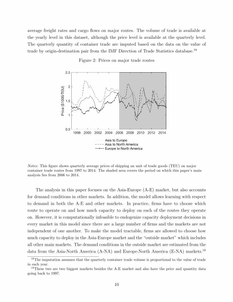
average freight rates and cargo flows on major routes. The volume of trade is available at

the yearly level in this dataset, although the price level is available at the quarterly level.

The quarterly quantity of container trade are imputed based on the data on the value of

trade by origin-destination pair from the IMF Direction of Trade Statistics database.18

Figure 2: Prices on major trade routes

Notes: This figure shows quarterly average prices of shipping an unit of trade goods (TEU) on majorcontainer trade routes from 1997 to 2014. The shaded area covers the period on which this paper’s mainanalysis lies from 2006 to 2014.

The analysis in this paper focuses on the Asia-Europe (A-E) market, but also accounts

for demand conditions in other markets. In addition, the model allows learning with respect

to demand in both the A-E and other markets. In practice, firms have to choose which

route to operate on and how much capacity to deploy on each of the routes they operate

on. However, it is computationally infeasible to endogenize capacity deployment decisions in

every market in this model since there are a large number of firms and the markets are not

independent of one another. To make the model tractable, firms are allowed to choose how

much capacity to deploy in the Asia-Europe market and the “outside market” which includes

all other main markets. The demand conditions in the outside market are estimated from the

data from the Asia-North America (A-NA) and Europe-North America (E-NA) markets.19

18The imputation assumes that the quarterly container trade volume is proportional to the value of tradein each year.

19These two are two biggest markets besides the A-E market and also have the price and quantity datagoing back to 1997.

10

These two markets along with the A-E market account over 50 % of all interregional trade

by volume and 67% by deployed ship capacity.

The reasons the analysis gives more attention on the Asia-Europe market are the fol-

lowing. First, it is the largest market in the container shipping industry accounting for over

23% of the total interregional container trade by volume and close to 40% in terms of the

deployed ship capacity. Second, it was most heavily impacted by the downturns in 2008, so

the effect of learning is likely to be more pronounced in this market. Figure 2 shows the

average prices on the five major trade routes by trade volume from 1997 to 2014. The shaded

area covers the 2006-2014 period on which the main analysis lies. The price fell by over 50

percent from the peak in 2007 to the trough in 2009 on the Asia to Europe route while it

fell by less than 30 percent on the Asia to North America route, which is the second largest

route.

Table 1: Descriptive statistics

Mean Std. Dev. Min MaxIndustry-level data (2006-2014)Shipbuilding price ($1000/TEU) 11.62 2.22 8.69 15.76Scrap price ($1000/TEU) 2.62 0.55 1.50 3.81

Market-level data (1997-2014)

Asia to EuropeQuantity (1 mil. TEU) 2.37 1.10 0.70 3.98Price ($1000/TEU) 1.51 0.28 0.80 2.09

Europe to AsiaQuantity (1 mil. TEU) 1.08 0.39 0.51 1.76Price ($1000/TEU) 0.78 0.10 0.57 1.07

Other routesQuantity (1 mil. TEU) 5.11 1.41 2.80 7.72Price ($1000/TEU) 1.36 0.12 1.06 1.60

Firm-level data (2006-2014)Capacity of owned ships (1m TEU) 0.30 0.25 0.04 1.47Capacity of ships in order book (1m TEU) 0.18 0.13 0.00 0.64Capacity of chartered ships (1m TEU) 0.31 0.29 0.01 1.55Capacity of ships deployed in Asia-Europe market (1m TEU) 0.22 0.19 0.04 0.99

Notes: There are 36 industry-level, 216 market-level, and 612 firm-level observations. Other routes includeAsia to North America, North America to Asia, North America to Europe, and Europe to North Americaroutes.

The analysis is further restricted to firms that deployed over 80,000 TEU of ships in the

Asia-Europe market on average in the 2006 to 2014 period. These firms account for more

than 95 percent of the total capacity of ships deployed in the Asia-Europe market. This

results in a quarterly panel of 17 firms from 2006 to 2014. There is no entry into or exit from

the Asia-Europe market by these firms in this period. Table 1 provides summary statistics of

this dataset. On average, firms in the sample own 300,000 TEU in capacity, charter 310,000

11

TEU and have an order book of 180,000 TEU.

Figure 3: The distribution of firm size

Notes: This figure shows the capacity owned by each firm as a percentage of total industry capacity, wherethe capacity is averaged over the period of 2006:Q1 to 2014:Q4.

Figure 3 shows the distribution of firm size based on the average owned capacity over

the period from 2006 to 2014. The market structure is quite concentrated with more than

40% of the total capacity concentrated on the top three firms in contrast to the bulk shipping

industry which consists of a large number of small ship-owning firms (Kalouptsidi (2014)).20

While there is considerable size variation among the top two firms, the rest of the firms are

similar in size.21

Before describing the model, I look for preliminary evidence of changes in firms’ in-

vestment policy. It is inherently difficult to test whether firms are adjusting their beliefs

about demand as they get new information since the beliefs are not directly observed. In-

stead, I search for suggestive evidence based on the difference in the predictions that a

full-information model and a learning model make. A learning model generally predicts that

even after controlling for the state (which includes all payoff-relevant variables), firms’ beliefs,

hence firms’ actions will be different before and after experiencing large demand shocks.22

20Kalouptsidi (2014) shows that the largest fleet share is 3% for Handysize bulk carriers.21The Herfindahl index for the industry is 970 when these 17 firms are accounted for.22The payoff-relevant variables are defined to be those variables that are not current controls and affect

the current profits of at least one of the firms as in Ericson & Pakes (1995) and Maskin & Tirole (2001).

12

By contrast, under full information firms’ perceived probabilities of transitioning to different

demand states from a given state stay fixed over time as new demand realizations do not

contain any new information. Hence, I examine whether firm behavior changes significantly

after firms experience large demand shocks. In particular, I test for a structural break in the

firm’s investment policy function and find evidence for such a break. The details of the test

and the results are provided in appendix B.

3 Model

This section presents the model for the container shipping industry. The model builds on

the dynamic oligopoly framework developed by Ericson & Pakes (1995) and the learning

literature in macroeconomics. Firms’ beliefs about demand change over time as firms re-

estimate the parameters of the demand process using up-to-date information available to

them. In each period a firm decides whether to invest in new ships and whether to scrap

existing ships based on its own capital and order book levels, and rivals’ aggregate capital

and order book levels as well as its beliefs about future demand. In the product market

competition stage, firms decide on how much capacity to charter (lease from a third-party

chartering company) and how much capacity to station in each market. I start by describing

the model of firm beliefs in section 3.1. Section 3.2 presents firms’ dynamic problem, and

section 3.3 demand for container shipping services and product market competition. Section

3.4 provides a definition of equilibrium.

3.1 A Model of Firms’ Beliefs about Demand

This section proposes an adaptive learning model of firms’ expectations about demand.

Section 6.1 presents details of all alternative models considered in this paper including a

full-information model, a Bayesian learning model, and a full-information model with time-

varying demand volatility. Under adaptive learning agents form expectations about demand

based on information available to them in each period. They operate like econometricians

who estimate the parameters of the model based on best information at their disposal and

make forecasts using their estimates.

Agents contemplate a first-order autoregressive model for demand in the Asia to Europe

market, denoted by zt, as the following:

zt = ρ0 + ρ1zt−1 + ωt (1)

= ρ′xt + ωt

13

where ωt ∼ N(0, σ2t ), ρ = [ρ0, ρ1]′, and xt = [1, zt−1]′. Similarly, the model for the demand in

the outside market (zt) is given as:

zt = ρ0 + ρ1zt−1 + ωt (2)

= ρ′xt + ωt

where ωt ∼ N(0, σ2t ), ρ = [ρ0, ρ1]′, and xt = [1, zt−1]′. In the full-information model, the

parameters in the demand model, {ρ0, ρ1, σ, ρ0, ρ1, σ} are known to the agents. By contrast,

under adaptive learning agents revise expectations by re-estimating these parameters in

each period based demand realizations up to time t, {zτ , zτ}tτ=0. At each t, firms’ beliefs

about demand can be described by the estimates of the AR(1) parameters, denoted as

ηt = (ρ0t , ρ

1t , σt, ρ

0t , ρ

1t , σt).

Firms are assumed to have homogenous beliefs about the aggregate demand and they

recognize this. The prices and quantities of container trade are public information period-

ically published in trade journals and other publications. Moreover, swings in global trade

demand common to all firms are the main source of demand shocks in this industry.23 The

model also assumes that agents do not internalize the possibility of learning in the future.24

In other words, firms use their current beliefs in forecasting demand. This assumption has

two behavioral interpretations. The first interpretation is that agents believe current beliefs

to be the correct forecasts for future demand. The alternative interpretation is that agents

use current beliefs in forecasting as these approximate future beliefs.

Let Xt = [x0, x1, ..., xt]′ and Rt =

X′tXt

t. The expectations at time t regarding the

Asia-Europe market demand under adaptive learning can be written recursively as

ρt = ρt−1 + λt(Rt)−1xt

(zt − ρ′t−1xt

)(3)

Rt = Rt−1 + λt(xtx′t −Rt−1) (4)

where λt is the weight parameter that governs how responsive the estimate revisions are to

new data. Figure 4 plots relative weights placed on observations for different values of λt.

23On a practical level there are no publicly available data that provide information on firm-level demand tomy knowledge, which are necessary to allow heterogenous firm beliefs. Nevertheless, heterogeneity in firms’beliefs would arise if firms experienced different demand shocks, for example, through different customerpools. How firms form heterogeneous beliefs and how they affect firm decisions and industry dynamics areinteresting topics of study for future work.

24This is often referred to as myopic learning in the literature. Suppose information is endogenous toagents’ decisions, for example, because agents are making consumption decisions for experience goods forwhich quality is difficult to observe in advance. In this case, the assumption of myopic learning rules outexperimentation, while allowing agents to internalize learning in the future may encourage experimentation.In this paper’s setting, since information about the aggregate trade demand is exogenous to agents’ actions,there is no room for experimentation regardless of the assumption on learning.

14

Figure 4: Weights on observations under adaptive learning

Nots: This figure plots weights that are applied to observations for different values of λt in the adaptivelearning model where λt is the weight parameter that governs how responsive estimate revisions are to newdata (see equation (3)).

For example, if λt = 1t, agents put equal weight on all observations in their information

set. If λt is some constant between 0 and 1, weights geometrically decline with the age of

the observation such that agents assign heavier weights to more recent observations. This

would be a natural way to form expectations if agents were concerned about the possibility

of structural changes (Evans & Honkapohja (2012)). A larger value of λt leads to heavier

discounting of older observations. For example, when λt = 0.03, agents put a 30% weight

on a 10-year-old observation relative to the most current observation, while when λt = 0.02,

agents put a 45% weight on a 10-year-old observation.

3.2 Firms’ Dynamic Problem

Time is discrete with an infinite horizon and is denoted by t ∈ {0, 1, 2, ...}. There are n

incumbent firms and the set of incumbent firms is denoted by N = {1, 2, ..., n}. Firms are

heterogeneous with respect to their firm-specific state, xit = (kit, bit), where kit is the capacity

of ships owned by firm i and bit is the backlog, or the capacity of firm i’s order book.25 The

25The owned capacity space denoted by K is discretized into 19 points such that K = {k0, k1, k2, ..., k18}and the order book capacity space denoted by B into 7 points such that B = {b0, b1, ..., b6}. K and B areboth discretized in 100,000 TEU increments such that k0 = 0 TEU, k1 = 100, 000 TEU, and so on, and

15

underlying industry state is st = ((xit)i, dt) where (xit)i is the list of all incumbents’ firm-

specific states and dt = (zt, zt) includes the demand states of the Asia-Europe market and

the outside market.

The timing of events is as follows: (1) Firms observe their current state as well as their

private cost shocks associated with investing and scrapping. They update their beliefs about

demand. (2) Firms make investment and scrapping decisions. (3) Firms choose how much

capacity to charter and how much capacity to deploy in the Asia-Europe market and the

outside market. They engage in period competition and receive period profits. (4) The

dynamic decisions are implemented and the delivery and depreciation outcomes are realized.

The industry evolves to a new state.

Computing a Markov perfect equilibrium (in which each incumbent firm follows a Markov

strategy that is optimal when all competitors firms follow the same strategy) is subject to the

curse of dimensionality. As the number of incumbent firms grows, the number of states grows

more than exponentially.26 To address this challenge, I consider an alternative equilibrium

concept which can be viewed in the context of the moment-based Markov Equilibrium (MME)

of Ifrach & Weintraub (2016), or more broadly the experience-based equilibrium (EBE) of

Fershtman & Pakes (2012).

In MME, firms keep track of and condition their strategies on the detailed state of

strategically important firms (dominant firms) and a few moments of the distribution de-

scribing non-dominant firms’ states, instead of the detailed state of all incumbents. This

reduces the size of the state space thereby alleviating the computational burden. My appli-

cation allows firms to keep track of their own firm-specific states, the sum of all incumbents’

states, and the aggregate demand states. Firms’ strategies thus depend on the firm-specific

state, xit = (kit, bit), and the moment-based industry state defined as st = (∑

i xit, dt). MME

strategies are not necessarily optimal, however; there may be a profitable unilateral deviation

to a strategy that depends on the detailed state of all firms. This is because the moment-

based state may not be sufficient statistics to predict the future evolution of the industry.

In appendix D.1, I consider a version that allows richer information by adding a dominant

firm’s state into the moment-based industry state and show that the model predictions are

robust to this change.

Firms make an investment decision (ιit ∈ {0, 1}) and a scrapping decision (δit ∈ {0, 1})in order to maximize expected discounted profits.27 I denote the strategy profile as µit =

b0 = 0 TEU, b1 = 100, 000 TEU, and so on.26There are 17 active firms in my application. Even a simple specification with a single state variable that

can take up to 5 different values would result in over a billion of states.27Firms are restricted to invest and/or scrap up to only one unit (100,000 TEU) per period. In the data

there are no observations of a capital reduction by more than one unit and there are only three instances

16

(ιit, δit). Each investing firm pays an investment cost. The investment cost consists of a part

common to all firms which is a function of the aggregate state, κ(st), and a privately observed

part of the cost, ειit ∼ N(0, (σι)2). If a firm decides to scrap its ships or if there is depreciation,

the firm receives a scrap value. The scrap value is the sum of the value common to all firms,

φ(st), and an iid private value distributed as εδit ∼ N(0, (σδ)2). Deprecation occurs with a

probability proportional to the firm’s current capital amount, given as ζkit for some constant

ζ.28 I denote as ν(δit, xit) the expected amount of capital reduction from depreciation or

scrapping before the realization of the depreciation outcome such that ν(δit, xit) is one if

δit = 1 and ζkit otherwise. The value function of a firm after observing its private shocks

and before making investment and scrapping decisions can be written as

V ηt(xit, st) = maxιit,δit

π(xit, st)− ιit (κ(st) + ειit) + ν(δit, xit)(φ(st) + εδit

)+βE [V ηt(xit+1, st+1|xit, st)]

where ηt is the vector of parameters summarizing firms’ beliefs in period t about future

demand. The value function is a function of ηt as it depends on how firms perceive the

demand state to evolve.

The current model does not allow for persistent heterogeneity in the investment costs

and scrap values across firms. The analysis of transaction-level pricing data on investment

and demolition confirms that there is no significant firm heterogeneity at least in the observed

transaction prices of investment and scrapping. The model incorporates firm heterogeneity in

other areas, however, since it may be important given the persistent concentration of market

power. First, the cost of chartering ships from a third party is allowed to depend on firm size,

since larger firms may have greater bargaining power over charterers. Second, the marginal

cost of production dethe capacity of firm’s deployed ships. The detailed specification of these

cost functions is given in section 3.3.

of an investment of more than one unit. Capping the maximum investment level to one unit for each firmreduces the action space thus alleviating the computational burden.

28If a firm scraps its vessels, there is no depreciation in the same period such that the maximum reductionin kit is one unit. This assumption is made since the data do not provide any observations of a capitalreduction by more than one unit. The interpretation of this assumption can be that when a firm decides toscrap its vessels, it chooses the oldest vessels that are about to deprecate on their own. This assumption canbe easily relaxed.

17

State Transitions

When a firm invests, the order book capacity increases by one unit when there is no delivery

at t and stays constant if there is delivery.29 A firm’s own capacity is determined by scrapping

decision, and depreciation and delivery outcomes. The transition of the firm-specific state is

described as:

kit+1 = kit + τit −min(δit + ψit, 1)

bit+1 = bit + µit − τit

where τit is delivery and ψit is depreciation. The probability of delivery is a linear function

of the firm’s order book capacity such that the delivery happens with the probability of ξbit

for some constant ξ. Similarly, the probability of depreciation is ζkit such that it linearly

increases in the capital stock. The perceived evolutions at time t of the aggregate demand

states for the Asia-Europe market and the outside market follow first-order autoregressive

processes as the following:

zt = ρ0t + ρ1

t zt−1 + ωt

zt = ρ0t + ρ1

t zt−1 + ωt

where ωt ∼ N(0, σ2t ) and ωt ∼ N(0, σ2

t ).30 This process is described in more detail in section

3.1. The parameters in the AR(1) model, ηt = (ρ0t , ρ

1t , σt, ρ

0t , ρ

1t , σt), summarize the beliefs

about the evolution of future demand at time t. How firms update these beliefs as they get

new information is described in section 3.1.

Note that even though the evolution of the underlying state st is a Markov process under

Markov strategies, the evolution of the moment-based industry state st may not be. This

is because information is lost in the process of aggregating information through moments.31

29This paper does not take into account the fact that ships are becoming larger and thus more efficient. Iinvestigate whether the improving efficiency of ships is the driving force in the investment boom and bustobserved in the data. I regress firm investment on the current size of the ships and other firm characteristicsand find that the current size is not a strong predictor of investment. It is possible to allow the efficiencyof ships to be an endogenous state variable. This would increase the sizes of the state space and the actionspace dramatically, however.

30I explore alternative specifications including a case in which the errors in the AR(1) processes followheavier-tailed t-distributions and a case in which correlation between demand in the Asia-Europe marketand demand in the outside market is allowed. Main results are robust to these alternative specifications.

31To understand this, suppose that there are three firms. Each of these firms keeps track of its ownfirm-specific state, xit and the sum of all three firms’ states as the moment-based industry state such thatst =

∑i xit. The underlying industry state is st = (xit)i. In one case, suppose that the underlying state is

(10, 10, 10), while in another case the underlying state (30, 0, 0). In both cases, the moment-based industrystate is st = 30. However, starting from these two different underlying states may not yield the same

18

Hence, I approximate the Markov process for the moments using empirical transitions fol-

lowing Ifrach & Weintraub (2016) and Fershtman & Pakes (2012).

Let µ denote the investment strategy and let Pµ′,µ denote the transition kernel of the

underlying state (xit, st), when firm i uses strategy µ′ and its competitors use strategy µ.

Then, we can define an operator Φ such that Pµ′,µ = ΦPµ′,µ where a Markov process Pµ′,µ

approximates the non-Markov process of the moment-based state, Pµ′,µ. In practice, the

moment-based industry state’s evolution is defined to be the long-run average of observed

transitions from the moment-based state in the current period to the moment in the next

period under strategy µ as follows:

Pµ[m′|s] = (ΦPµ)[m′|s] = limT→∞

I{st = s, mt+1 = m′}∑Tt=1 I{st = s}

where mt = (∑

i xit) includes the moments in the moment-based state.

3.3 Demand for Container Shipping and Product Market Compe-

tition

In each period, firms choose (a) how much capacity to charter (hit), and (b) how much

capacity to allocate to the Asia-Europe market (qit) and the outside market (qit) given the

state they are in. In other words, a firm chooses how much of its total capacity to allocate

to the Asia-Europe market or the outside market where the total capacity is determined

as the sum of its chartered and owned capacity. The capacity firms allocate to the Asia-

Europe market determines the supply in the market, which along with demand determines

the market-clearing price and quantity. Demand for each route in the Asia-Europe market

is assumed to have constant elasticity as follows:

logQjt = zjt + α1 logPjt (5)

where zjt denotes the demand state, Pjt the price, and Qjt the quantity of route j at time t.

The marginal cost of providing services on a route is linearly increasing in quantity up

to the firms’ capacity constraint as follows:32

mc(qijt, qit) =

a+bqijtqit

if qijt ≤ qit

∞ otherwise.(6)

distribution for the moment-based state in the next period (st+1).32This functional form assumption is based on the fact that it becomes increasingly hard to schedule

loading and unloading as the ship reaches its full capacity.

19

Then, the supply curve for route j is given as the horizontal sum of all firms’ supply curves

as follows:

Pjt = a+bQjt

Qt

if Qjt ≤ Qt (7)

where Qt =∑

i qit. The price in the Asia-Europe market is determined by the intersection

of the demand curve given in equation (5) and the supply curve given in equation (7).

The period profit is the sum of profits from providing shipping services on the Asia to

Europe route and the Europe to Asia route plus the profit from the outside market minus

the charter cost and the fixed cost of capital:

π(xit, st) = maxqit,hit

( ∑j∈{1,2}

Pjtqijt − c(qijt, qit))

+R(qit, Qt, st)− CC(hit, xit, st)− FC · kit

(8)

where FC is the fixed cost of holding one unit of capital, R is the profit from the outside

market, CC is the charter cost, and qit is the capacity deployed in the outside market. The

fixed cost of holding ships includes all costs that do not vary with the output level (or how

full the ships are) such as docking fees, maintenance costs, canal dues, and port charges. I

do not explicitly model the chartering market and the product market competition in the

outside market but account for them in a reduced form way. The detailed specification of the

reduced-form functions for the charter cost and the outside-market profit is given in section

5.2.

3.4 Equilibrium

The value function can be re-written as the perceived value of a firm using moment-based

strategy µ′ in response to all other firms following strategy µ:

V ηµ′,µ(x, s) = π(x, s)− ι (κ(s) + ει) + ν(δ, x)

(φ(s) + εδ

)+ βEµ′,µV

η(x′, s′|x, s).

The definition of an equilibrium is then given as follows.

Definition Equilibrium comprises of an investment and scrapping strategy µ that satisfies

the following conditions:

(a) Firm strategies satisfy the optimality condition:

supµ′∈M

V ηµ′,µ(x, s) = V η

µ (x, s) ∀(x, s) ∈ X × S.

20

(b) The perceived transition kernel is given by:

Pµ = ΦPµ

Equilibrium is computed using an algorithm based on value-function iteration. Appendix C

describes the algorithm in detail.

4 Empirical Implementation of the Learning Model

This section discusses the implementation of the learning model described in section 3.1

and presents expectations about demand implied by the model (see section 6.1 for the im-

plementation of all alternative models of firm beliefs). The truncated nature of the price

and quantity data for container trade poses a challenge in implementing the learning model.

An agent’s information set in each period includes all observations from the past. How-

ever, although firms may have access to observations from the inception of the industry,

the researcher may not. This problem arises in most empirical settings when dealing with

a learning model. In my particular setting, data on prices and quantities for major trade

routes are available starting from 1997, although the first international voyage dates back to

1966. Given this challenge, I explore two alternative methods of empirically implementing

an adaptive learning model: the truncation approach and the imputation approach.

The truncation approach entails setting the initial period of the information set as the

start date of the data. This method is straightforward to implement and is appropriate if

firms also do not have access to information beyond the data available to the researcher.

However, bias can arise if agents’ information set includes observations going further back

than the start date of the data. The bias would be mitigated as agents discount older

observations more heavily when forming expectations.

This approach is implemented as follows. The set of weight parameters (λt) that I

consider is {1t, 0.01, 0.02, 0.03, 0.04}.33 If λt = 1

t, equal weights are applied to all past ob-

servations. In practice, the estimation procedure under this parameter value amounts to

applying least squares to estimate equation (1) for each period separately. The regression

at period t uses demand state data covering from the start date of the data to the current

period t, or {zτ , zτ}tτ=0 where the steps of recovering these data are provided in section 5.1.

If λt is a constant, weights on observations geometrically decline with the age. In this case,

weighted leasts squares are applied where the weight on an observation from the period τ is

33Orphanides & Williams (2005) suggest that the constant gain parameter in the range between 0.01 and0.04 match the data on expectations well.

21

given by (1− λt)t−τ .The imputation approach employs external data that provide information about the

missing data. This approach is appealing if agents indeed use longer historical data in

forming expectations than observed and the researcher has access to the external data that

provide a good approximation to that data. Bias can arise, however, from the imputation

process depending on the quality and scope of the external data. For this paper’s setting,

one could consider using international trade data to proxy demand for container shipping.

The imputation approach is implemented as follows. I set the start date for firms’

information as the second quarter of 1966, which is the date of the first international container

voyage. Then, I employ quarterly data on the value of trade by origin-destination pair from

the IMF Direction of Trade Statistics database to impute the missing data on demand states

from 1966:Q2-1996:Q4.34 Finally, I estimate the beliefs using the imputed longer time-series

data in the same way as the truncation approach.

The truncation approach is adopted in the end because it provides a better data fit.

Moreover, it can be more universally applied since the imputation method requires some

external data which are not always available. Figure 15 in appendix D.2 compares beliefs

under the two approaches.

Figure 5: Beliefs under Learning for the Asia-Europe Market

Notes: This figure shows firms’ beliefs about demand in the Asia-Europe market for 2000:Q1 to 2014:Q4under adaptive learning with λt = 0.02. The beliefs are summarized by the three parameters, {σt, ρ0t , ρ1t},in the AR(1) process as given in equation (1). Beliefs for 2006-2014 in the shaded area are used in themain analysis.

Figure 5 shows firms’ demand parameter estimates from 2000 to 2014 under adaptive

34To translate the value of trade to the quantity of container trade, the demand state for the 1997-2014period was regressed on the de-trended value of trade. Then, the demand states for periods with missingdata are constructed as predicted values from the regression. For the 1997-2014 period, actual demand statesare used.

22

learning with λt = 0.02 for the Asia-Europe market (see figure 11 in appendix A.1 for the

outside market). The estimates in the shaded area are for 2006 to 2014, which will used in

the estimation of the dynamic model. The estimate of the persistent parameter ρ1t rises from

2006 to 2007 and shows a general downward trend thereafter. The variance parameter σt

hikes in early 2009 and stays high throughout the end of the sample period.

Under adaptive learning, the degree to which the parameter estimates react to recent

events grows as agents put more weights on recent observations (as shown in figure 12 in

appendix A.1). For example, the degree to which σt jumps around 2009 is the smallest in

the case where agents weigh all past demand realizations equally (λt = 1/t). When λt is

a constant, the larger λt, the larger the jump in σt around 2009. Similarly, the larger the

fall in the persistence parameter ρ1 in the post-2008 period, the larger λt becomes. It is

this variation in beliefs and the variation in the data in investment and scrapping around

demand shocks that identify the model of firm beliefs.

5 Estimation and Empirical Results

The estimation of the dynamic model of investment with learning proceeds as follows. First,

I estimate demand for shipping services to recover the elasticity of demand and demand

states. Second, I estimate parameters governing static competition including the marginal

cost of production, the charter cost, and the outside market profit, which are used to compute

period profits. Third, I estimate the investment cost and the scrap value based on the pricing

data of shipbuilding and demolition as well as other model primitives such as the delivery

and depreciation processes. Lastly, I estimate the dynamic model including the model of

firm beliefs through the method of simulated moments.

5.1 Estimating Demand for Shipping Services

The goal of this section is to estimate the price elasticity of demand and to construct demand

states for the Asia-Europe market and the outside market.35 The empirical analogue of the

constant elasticity demand model in equation (5) is:

logQjt = α0 + α1 logPjt + α2Wjt + εjt (9)

where j is an indicator for trade routes, Qjt is the amount of container shipping services in

terms of TEU, Pjt is the average price per TEU, and Wjt is a demand shifter. I estimate

35This section follows the demand estimation of Kalouptsidi (2014) closely.

23

equation (9) using instrumental variables regression in order to correct for the endogeneity

of prices. The price is instrumented with the average size and age of ships and the fraction

of ships that are over 20 years old. The size of ships is one of the key determinants of cost

efficiency as larger ships require less fuel per TEU on average. The age of ships matters as

well, since older ships tend to require higher maintenance costs. Log GDP for the destination

area is used as a demand shifter.

The estimation uses data from six major trade routes from 2001:Q2 to 2014:Q4.36 The

demand parameters are identified by the time-series variation as well as the cross-sectional

variation across six different routes in the data along with the constant elasticity functional

form assumption. In particular, since ships have to go back and forth the two routes in

each market they serve, two routes in the same market (e.g. Asia to Europe and Europe to

Asia) have the same level of supply while facing different demand shocks, which helps the

identification of the demand parameters.

The price elasticity of demand is estimated to be -3.89 (see table 8 in Appendix A.1

for detailed results). This implies that a change in price from $1510 per TEU to $1360 per

TEU would result in a change in quarterly quantity demanded of approximately 0.92 million

TEU on the Asia to Europe route.37

Given the elasticity of demand estimates, I construct the demand state for each trade

route (zjt) as the intercept of the demand curve:

zjt = α0 + α2Wjt + εjt (10)

where {α0, α2} are parameters estimated from the regression and εjt is the residual. Finally,

I construct aggregate demand states for the Asia-Europe market and the outside market

from the route-level demand. For the Asia-Europe market, I take the demand state for the

Asia to Europe direction. Since the container trade volume is less than half on the Europe to

Asia direction, firms’ investment and capacity deployment decisions in the market are mostly

dictated by the trade demand on the Asia to Europe direction. For the outside market, I

take the sum of the demand states in the non-Asia-Europe routes. Figure 6 plots the demand

states for 1997 to 2014 for the Asia-Europe and the outside markets. There is a large drop

in demand in both markets in late 2008 to 2009. In the Asia-Europe market, the boom and

36Although the price, quantity, and GDP data available from 1997, the instruments are available startingfrom 2001:Q2. The included trade routes are Asia to Europe, Europe to Asia, Asia to North America, NorthAmerica to Asia, Europe to North America, and North America to Europe.

37Stopford (2009) explains that container trade is price elastic because lowering prices encourages thesubsitution of cheap foreign substitues for local products. Moreover, other transportation modes are availablesuch as road and rail transportation and air freight. Kalouptsidi (2014) estimates the price elasticity ofdemand for bulk shipping to be -6.17 under a constant elasticity specification.

24

Figure 6: Demand states

bust cycles in demand are shorter in length after 2008.

5.2 Estimating the Profit Function

The second step of the estimation is to construct period profits by estimating the marginal

cost, charter cost, and outside market profit functions. Firms’ capacity deployment decisions

yield a supply curve which along with the demand curve determines the equilibrium prices

and quantities for the Asia-Europe market. The marginal cost of providing container shipping

services is specified in equation (6), which serves as the basis for the maximum likelihood

estimation of the cost parameters (a, b).

The outside market profit and the charter cost functions are specified in a reduced-form

way as:

R(qit, xit, st) = qit

(r0 + r1zt + r2Qt

)CC(hit, xit, st) = hit(γ0 + γ1zt + γ2kit + γ3Kt).

The profit from each unit of capacity deployed in the outside market is allowed to depend on

the total deployed capacity in the outside market (Qt) since higher supply may lead to fiercer

price competition and lower profit. The charter cost depends on the firm-level own capacity

(kit) since larger firms may get discounts on charter rates. The charter cost is also allowed

to depend on the total capacity owned by operator (Kt) as it is likely to affect demand for

25

chartering.

The estimation of the charter cost and outside market profit functions is based on firms’

static profit maximization problem. Given the demand estimates and the first-order condi-

tions with respect to the capacity deployed on Asia-Europe route (qijt) and the chartering

decisions (hit), I estimate the charter cost and the outside-market profit functions via maxi-

mum likelihood. The variations in capacity deployment and charter decisions across different

firm types and across time along with the first-order conditions and the functional form as-

sumptions provide identification for these parameters.

Table 9 in Appendix A.1 reports the estimates of the profit function parameters. The

coefficients on the Asia-Europe market demand state in the outside market profit and charter

cost functions (r1 and γ1) are positive. This implies that stronger demand leads to higher

outside market profits as well as higher charter costs. The estimates also show that when

there is more aggregate deployed capacity in the outside market, firms earn less from that

market on average. In addition, larger firms tend to face lower charter costs, and an increase

in total industry capacity owned by ship operators lowers charter costs.

5.3 Estimating Other Model Primitives

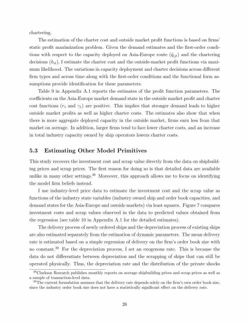
This study recovers the investment cost and scrap value directly from the data on shipbuild-

ing prices and scrap prices. The first reason for doing so is that detailed data are available

unlike in many other settings.38 Moreover, this approach allows me to focus on identifying

the model firm beliefs instead.

I use industry-level price data to estimate the investment cost and the scrap value as

functions of the industry state variables (industry owned ship and order book capacities, and

demand states for the Asia-Europe and outside markets) via least squares. Figure 7 compares

investment costs and scrap values observed in the data to predicted values obtained from

the regression (see table 10 in Appendix A.1 for the detailed estimates).

The delivery process of newly ordered ships and the depreciation process of existing ships

are also estimated separately from the estimation of dynamic parameters. The mean delivery

rate is estimated based on a simple regression of delivery on the firm’s order book size with

no constant.39 For the depreciation process, I set an exogenous rate. This is because the

data do not differentiate between depreciation and the scrapping of ships that can still be

operated physically. Thus, the depreciation rate and the distribution of the private shocks

38Clarkson Research publishes monthly reports on average shipbuilding prices and scrap prices as well asa sample of transaction-level data.

39The current formulation assumes that the delivery rate depends solely on the firm’s own order book size,since the industry order book size does not have a statistically significant effect on the delivery rate.

26

Figure 7: Predicted Investment Costs and Scrap Values

(a) Investment Costs (b) Scrap Values

Notes: The left panel shows the average shipbuilding price observed in the data and the predictedshipbuilding price from the regression of the shipbuilding price on the industry state variables. The rightpanel shows the average scrap value and the predicted scrap value.

to the scrap value can not be separately identified. The depreciation rate, ζ, is set such that

the average age at which ships naturally depreciate is 20 years.40

5.4 Estimating the Dynamic Model of Investment with Learning

The last and most computationally intense step of the estimation entails estimating the model

of firm beliefs and the dynamic parameters. The typical empirical strategy of estimating a

dynamic game of investment is to recover objects like investment costs, entry costs, and exit

values by searching for parameters that minimize the distance between actions observed in

the data and the ones that the parameters imply (e.g. Ryan (2012) and Collard-Wexler

(2013)). This paper instead employs data on shipbuilding and demolition prices to estimate

investment costs and scrap values as described in section 5.3, which opens up the possibility

to identify the model of firms beliefs. Although the application is different, the underlying

logic of this approach is similar to that of Hortacsu & Puller (2008) in which the authors use

marginal cost data to quantify how much firms’ bidding deviates from the optimal bidding

benchmark.

I employ the method of simulated moments (MSM) to estimate the dynamic model,

which minimizes a distance criterion between key moments from the actual data and the

40Although historically the lifespan of container ships was 25 to 30 years, it has fallen in recent yearsespecially for larger ships. Vesselvalues reports that the the average age of all sizes of container ships soldfor scrap was around 22 years old and the average age at which Post-Panamax container ship was sold forscrap was around 19.5 years.

27

simulated data. Let θ denote the vector of dynamic and belief parameters such that θ =

(σι, σδ, FC, λt). I solve for an equilibrium of the dynamic investment model and obtain the

optimal investment policy function for each candidate parameter vector.41 Using equilibrium

strategies obtained in the previous step, I simulate the equilibrium path for the 2006 to 2014

period S = 1000 times. And from these paths, I obtain the simulated moments as follows:

Γ(θ) =1

S

S∑s=1

Γs(θ).

I search for the parameter vector that minimizes the weighted distance between the data

and simulated moments given as:

f(θ) =(Γd − Γ(θ)

)′W(Γd − Γ(θ)

). (11)

where Γd is the set of data moments.42

The identification relies on a revealed-preference argument. I have recovered the values

of benefits and costs of each of the options that the firm faces–investment, scrapping, and

staying for each state in the state space as described in section 5.3. As a result, given

these values, firms’ choices in various states observed in the data reveal their expectations

about future demand. More concretely, the estimation relies the variation in firms’ beliefs

across different learning parameter values and the variation in firm behavior across time and

firms observed in the data. As firms discount older observations more heavily, their beliefs

become more responsive to recent shocks. This leads to different predictions about, for

example, the effect of recent demand shocks on investment and the duration of the impact

of demand shocks. In principle, the parameters are identified by both time-series and cross-

sectional variations. Nevertheless, the main source of identification is time-series variation

in investment and scrapping as well as investment costs and scrap values. And it is essential

to observe a boom and a bust in my sample period. The shipping industry provides a great

setting in that it is exposed to large exogenous fluctuations in demand coming from cycles

41Recently, empirical techniques have been proposed to estimate the dynamic industry equilibrium withouthaving to solve for an equilibrium (e.g. Aguirregabiria & Mira (2007), Bajari et al. (2007), Pakes et al.(2007)). The first stage of this approach entails recovering firms’ policy functions by regression observed

actions on observed state variables. The second stage involves estimating structure parameters which makethese policies optimal. This approach relies on flexible functional forms in the first step, so the data require-ment is too high given the global nature of my data set. I use a full solution method instead, which involvessolving the model at every guess of the parameter but is more efficient.

42The search is done over grids of (σι, σδ, FC, λt). The grids for σι and σδ are in increments of 0.005and the grid for FC is in increments of $50/TEU. The set of candidate belief parameter values is λt ∈{ 1t , 0.01, 0.02, 0.03, 0.04}. I use the inverse of the variance-covariance matrix of the simulated moments asthe weighting matrix (W ).

28

in world trade.

The moments used in the estimation include the average investment before and after

2008, the volatility of investment, the correlation in demand and investment, and the aggre-

gate capacity of owned and backlogged ships. Table 2 lists these moments and compares the

data moments and simulated moments under the parameter estimates.

Table 2: Data and Simulated Moments

Data moments Simulated moments

Average investment in 2006-2008 (1 mil. TEU) 0.23 0.23(0.03)

Average investment in 2009-2014 (1 mil. TEU) 0.14 0.15(0.02)

Total capacity of owned ships (1 mil. TEU) 5.09 5.15(0.27)

Total capacity in the order book (1 mil. TEU) 3.07 2.98(0.14)

Correlation between demand and investment 0.19 0.22(0.12)

Volatility of investment (1 mil. TEU) 0.17 0.17(0.03)

Notes: This table compares moments observed in the data and moments simulated under the estimatedparameters. The simulated moments are computed based on 1000 series of equilibrium paths. Standarddeviations are in parentheses.

Table 3: Dynamic Parameter Estimates

λt 0.02 (0.005)σι (1 bil. US dollars) 0.275 (0.055)σδ (1 bil. US dollars) 0.43 (0.092)FC (1 bil. US dollars) 0.025 (0.0051)

Notes: This table shows estimates of dynamic parameters. λt is the weighting parameter in the adaptivelearning model which governs how heavily agents discount older observations when forming expectationsabout demand. σι is the standard deviation of the i.i.d. shock around the investment cost of building100,000 TEU and σδ around the scrap value. FC is the fixed cost of holding capacity of 100,000 TEU.Standard errors are in parentheses.

My estimates, reported in table 3, indicate that the adaptive learning model with λt =

0.02 provides the best fit to the observed data moments, which I will refer to as the baseline

learning model in the rest of the paper. This implies that agents put approximately 45%

weights on a 10-year-old observation compared to the most recent observation. This estimate

is very close to the values that previous studies in macroeconomics have estimated based

29

Figure 8: Model Fit of the Learning Model

(a) Capacity of Owned Ships and Order book (b) Yearly Investment

Notes: The left panel shows the industry evolution simulated under the baseline learning model (adaptivelearning with λt = 0.02) and the industry evolution in the data. The right panel shows yearly investmentsimulated under the baseline learning model and observed in the data, respectively. The simulatedmoments are based on 1000 equilibrium paths.

on aggregate survey data such as the Survey of Professional Forecasts or micro data on

expectations. For example, Malmendier & Nagel (2016), Milani (2007), and Orphanides &

Williams (2005) estimate the constant-gain parameter (λt) to be 0.0175, 0.0183, and 0.02,

respectively, with respect to expectations about macroeconomic conditions and monetary

policy. Figure 8 shows that the baseline learning model does well at predicting the investment

boom in 2007 and the plunge in investment in 2009.

The fixed cost of holding one unit of capital (100,000 TEU) in one quarter is estimated

to be 25 million dollars, which is approximately 36% of the period’s profit from one unit of

capital (where the period profit is the sum of profits from the Asia-Europe market and the

outside market minus the charter cost and does not include the investment cost and scrap

value). This fixed cost includes all costs that owning and operating ships impose regardless

of the production level such as maintenance costs, canal dues, and port charges. It also

includes the cost of labor needed in the operation of the ships regardless of how full the ships

are.

30

6 Alternative Models of Firm Beliefs and Model Diag-

nosis

So far this paper has considered an adaptive learning model. In section 6.1, I consider various

alternative models for firms’ belief-formation process. This serves as a robustness check for

the baseline model. Moreover, the comparison of the estimation results under learning and

full information will shed light on the role of learning. Comparing model fits across different

models of firm beliefs, however, hinges on the assumptions made in various parts of the

model and the structural estimation. In section 6.2, I discuss a way of diagnosing these

models based on GDP forecast data which relies less heavily on modeling assumptions

6.1 Alternative Models of Firm Beliefs

The models of firm beliefs considered in this section include: a full-information model with

constant volatility; a Bayesian learning model; and a full-information model with time-

varying volatility. This section presents model specifications, firm beliefs implied by each

model, and estimation results.

Full Information

Agents contemplate a first-order autoregressive model for demand in the Asia to Europe

market and the outside market given by equations (1) and (2) as in the adaptive learn-

ing model. In the full-information model, however, the parameters in the demand model,

{ρ0, ρ1, σ, ρ0, ρ1, σ}, are known to the agents. Then, estimating beliefs under the full-information

model involves estimating the demand process using the full sample of data or as much data

as available to the researcher. I apply least squares to estimate the AR(1) processes using

data from 1997:Q1 to 2014:Q4. Beliefs implied by the full information model as well as beliefs

under the Bayesian learning model discussed later in this section and the baseline learning

model are presented in figure 9. The parameter estimates stay constant under full informa-

tion by construction. Compared to the baseline learning model, the volatility estimate (σ)

is higher and the persistent parameter (ρ1) lower in the pre-2008 period.

Figure 10(a) shows the annual investment levels predicted by the full-information model

in comparison with those observed in the data. This model fails to predict the correct quan-

tity and timing of investment. Specifically, it predicts that firms restrain from investing in

the high demand period of 2006-2007 and invest more heavily in the post-2008 period. This

happens for the following reason. A demand increase for shipping has two opposing forces

on investment. On one hand, investment becomes more costly as increased demand for new

31

Figure 9: Beliefs under Alternative Models of Beliefs for the Asia-Europe Market

Notes: This figure shows firms’ beliefs about demand in the Asia-Europe market for 2000:Q1 to 2014:Q4under the full-information, Bayesian learning, and baseline learning (adaptive learning with λt = 0.02)models. The beliefs are summarized by the three parameters, {σt, ρ0t , ρ1t}, in the AR(1) process as given inequation (1). Beliefs for 2006-2014 in the shaded area are used in the main analysis.

Figure 10: Model Fits under Alternative Models of Firm Beliefs

Notes: This figure shows yearly investment observed in the data and predicted by each of the alternativemodels of firm beliefs. The simulated moments are based on 1000 equilibrium paths.

ships leads to a higher volume of backlogs. On the other hand, high demand raises returns

to investment, raising demand for new ships. The positive demand-side effect is dominated

by the negative supply-side effect resulting in firms investing more under weak demand con-

ditions in this particular case. The positive effect is weaker under full information, because

while high demand shocks make firms revise their expectations upward under learning, this

32

is not the case under full information. As shown in figure 9, in 2006-2007 firms are more pes-

simistic and perceive the volatility of demand to be higher under full information compared

to in the learning model.

Bayesian Learning

Under Bayesian learning, each firm starts with prior beliefs about the parameters of the

model. Then, based on its information set, {zτ , zτ}tτ=0, the firm updates its beliefs about

the parameters in the demand process, (ρ0t , ρ

1t , σt, ρ

0t , ρ

1t , σt). The AR(1) coefficients for the

Asia-Europe market, ρ = [ρ0, ρ1], have normal priors given by ρ0 ∼ N(µ0,Σ0). The prior of

σ2 follows an inverse Gamma distribution. Then, the posterior distribution ρt ∼ N(µt,Σt)

has the mean and the variance given by

µt = Σt

(Σ−1

0 µ0 + σ−2(X ′tZt))

Σt =(Σ−1

0 + σ−2(X ′tXt))−1

.

The beliefs are defined similarly for the outside market.

The first three years of the price and quantity data (1997:Q1-1999Q4) are used in the

estimation of the prior beliefs.43 I start from diffuse priors and apply the Gibbs sampling

methods (see table 11 in appendix A.2 for the estimates). In the first quarter of 2000, firms

start with the prior beliefs about the parameters and revise their beliefs using Bayesian

updating in each period based on newly realized data. I apply the Gibbs sampling techniques

to estimate the posterior beliefs.

Figure 9 shows beliefs under Bayesian learning. Compared to the baseline model of

adaptive learning, the degree to which firms’ beliefs react to new data is smaller under

Bayesian learning. This is because there are less weights placed on new data under Bayesian

learning as agents place positive weights on their prior beliefs. Consequently, although the

Bayesian learning model correctly predicts the timing of the investment boom and bust, the

magnitudes of the rise and the fall in investment are smaller as shown in figure 10(b).

Full Information with Time-Varying Volatility

This paper has considered only homoskedastic models so far. However, changes in demand

volatility may also be able to explain firms’ investment behavior without the need to intro-

duce parameter learning in the model. Therefore, I consider a full-information model with

43I also explore using the full sample from 1997 to 2014 for estimating the priors.

33

a more flexible specification of the variance of the model: the GARCH model.44 Demand is

assumed to follow the same AR(1) process as in other models. But volatility is assumed to

follow a GARCH(1,1) process such that the current period’s variance depends on the last

period’s realized error and variance:

σ2t = a0 + a1ω

2t−1 + b1σ

2t−1

where ωt−1 is the realized error in period t− 1.

The GARCH model is estimated using the full sample of data (1997:Q1-2014:Q4). The

estimates are presented in table 12 and the inferred conditional variance in figure 13 in

appendix A.2. Compared to the volatility estimate in the learning model, the increase in the

variance around 2009 is larger. But the increase is more temporary unlike in the learning

model where the variance remains high through the end of the sample period.

The dynamic model presented in section 3.2 is modified to accommodate time-varying

volatility. Since firms need the current period’s variances and errors and the GARCH model

parameters as well to predict the next period’s variance, these parameters are included as

state variables. As shown in figure 10, the time-varying volatility model predicts the invest-

ment patterns in the data better than the full-information model with constant volatility,

in particular the timing of the investment boom and bust. Nevertheless, the magnitude of

the investment cycles is smaller compared to observed in the data or predicted by the adap-

tive learning model. This finding provides some insights into firms’ beliefs about demand.

It shows that the low volatility in demand in the pre-2008 period and a sharp increase in

volatility in 2009 help us explain the high level of investment in the pre-2008 period and

the subsequent fall in investment. Nonetheless, the finding also suggests that changes in the

level of demand forecasts in addition to the changes in the variance may be necessary to

correctly predict firms’ investment behavior.

6.2 Diagnosing Models of Firm Beliefs using GDP Data

In this section, I employ an alternative strategy to diagnose different models of firm beliefs.

In particular, based on the fact that GDP and trade demand are highly correlated, I examine

which model of firm beliefs generates beliefs that are most consistent with GDP forecasts.

The ECB publishes the Survey of Professional Forecasters (SPF) for the euro area quarterly

and reports the mean forecast of one-year-head and two-year-ahead GDP growth rates as

44As an alternative model of stochastic volatility, I consider a regime-switch mode where the variance isno longer a constant but can take on one of two values σt ∈ {σl, σh} and state changes are governed by aMarkov transition matrix. I omit details of this model as it produces similar results as the GARCH model.

34

well as a measure of how uncertain each forecaster is about his or her forecast. For the

uncertainty measure, each forecaster is asked to allocate subjective probabilities to ranges

of possible outcomes with a width of 0.5 percentage point.45

I take the forecast for the 2-year ahead GDP growth to construct the mean and the

variance of the forecasts in each quarter from 2006 to 2014.46 Then, I construct the mean

and the variance of 2-year ahead demand growth that each model of beliefs implies. Finally,

I compute correlation between the mean and the variance of GDP forecasts and the mean

and the variance of demand forecasts implied by each model of beliefs. The correlation

coefficients are reported in table 4.

Table 4: Correlation between GDP Forecasts and Demand Forecasts

Full info Full info Bayesian Adaptive learningCorrelation coefficient GARCH learning λt = 1

t λt = .01 λt = .02 λt = .03

Between means of GDP -0.23 -0.23 0.14 0.19 0.20 0.21 0.22& demand growth (0.17) (0.17) (0.17) (0.17) (0.17) (0.17) (0.17)Between variances of GDP . 0.37 0.83 0.86 0.86 0.85 0.83& demand growth (0.16) (0.09) (0.09) (0.09) (0.09) (0.10)

Notes: The mean and variance of GDP growth forecasts are based on two-year ahead forecasts publishedby the ECB.

The results confirm that the adaptive learning model produces beliefs that are most

highly correlated with beliefs implied by GDP forecasts (although the exercise does not

reveal which value of λt produces the most favorable outcome). The correlation coefficient

for the mean growth is approximately 0.20 for adaptive learning and 0.14 for Bayesian

learning. The correlation for the variance ranges from 0.83 to 0.86 for the learning models.

By contrast, the correlation for the mean is negative for the full-information models as they

predict that the growth rate is higher during periods of weak demand.47 In addition, under

full information with constant volatility the correlation for the variance is zero since the

variance is constant by construction. The correlation coefficient is 0.37 under the GARCH

model, which is still significantly lower than under learning models.

45For example, forecasters are asked to assign a probability to real GDP rising between 0.0% and 0.4%,0.5% and 0.9%, and so on.

46Only two-year ahead forecasts are used in the analysis because there is substantial bunching in theforecasters’ probabilities in end bins for one-year forecasts. The bunching makes it difficult to constructvariance estimates.

47This is because the AR(1) process has the mean-reversion property. So with the constant parameterestimates as in the full-information model, the expected growth rate is larger when current demand is lower.

35

7 Counterfactual Analysis

In this section, I address various firm-strategy and public-policy issues and assess the role

of learning through counterfactual experiments. In the first set of counterfactuals, I con-

sider policies that lessen competition and allow coordination among firms by simulating the

industry under a multi-plant monopolist and the merger of top two firms. By doing so, I

investigate how competition and strategic incentives affect investment and whether increased

coordination among firms could have curtailed industry oversupply. Furthermore, I compare

results from conducting these experiments under learning and full information to understand

how the competitive forces interact with learning. In the second set of counterfactuals, I

address the long-standing question on the effect of demand volatility on investment. By ap-

plying the learning framework I shed light on the new informational channel through which

demand fluctuations affect investment. Lastly, I simulate a scrapping subsidy policy. This

policy makes investment more reversible as it helps firms to scrap ships at a higher rate when

demand conditions worsen. This policy may therefore help firms deal with excess capacity.

It may also encourage investment, however, as it raises the value of owning ships.

7.1 Coordination among Firms

In this section, I study the effects of strategic incentives and consolidation as well as how

the effects interact with agent beliefs arising from learning. To deal with the recent excess

capacity in the industry, container shipping firms have increasingly moved towards consolida-

tion. Maersk Line and MSC–the world’s two biggest container-shipping companies-formed

an alliance named 2M, which akin to a code-sharing deal between airlines, was meant to

help firms cut costs by using each other’s ships and port facilities and reduce competition.

More firms are planning mergers and acquisitions as well. Cosco and CSCL, the sixth and

seventh largest carriers by operated fleet capacity, have proposed a merger. CMA-CGM has

proposed an acquisition of APL.

On one hand, increased consolidation may hurt consumers through reduced competition.

On the other hand, there are potential sources of efficiency gains on the producers’ side, which

makes the final direction of the welfare change ambiguous. In particular, consolidation may

reduce the business stealing effect and preemption motives that can lead to the capital level

that is higher than the socially optimal level.48

48Mankiw & Whinston (1986) show that the business stealing effect can result in socially inefficient levelsof entry when there are fixed costs of entry. Also, many theoretical studies predict that strategic incentivescan lead to excess capacity, since firms may use investment as a commitment to deter entry or expansion ofrivals (e.g. Spence (1977)).

36

My model incorporates several sources of strategic incentives. First, there is a business-

stealing effect. A firm’s deployment of an extra unit of capacity has a negative effect on the

market price and the competitors’ profitability. The business-stealing effect arises because

this negative effect of increasing one’s own capital is internalize by all incumbents in the

market. Second, as the volume of the industry order book grows and shipyards get closer

to their full capacity, the price of building a new ship increases. This generates dynamic

incentives for firms to preemptively commit to investment before others do when they expect

strong demand.

I first consider a monopolist who operates and makes joint decisions of investment,

scrapping, chartering, and deployment for all firms in order to maximize the aggregate profits.

I assume that the monopolist operates multiple plants while maintaining the same firm size

distribution as observed in the data instead of assuming that the monopolist operates all

ships under one entity. This helps disentangle the effect of strategic incentives from the

effect arising from a change in the firm size distribution, for example, through cost savings,

changes in bargaining power, etc. The monopolist is endowed with beliefs from the baseline

learning model. Similarly, in a merger counterfactual, I allow the joint profit maximization

of the top two firms.

Removing competition externalities through the monopoly case has a substantial effect

on investment: during the period of 2006 to 2014, investment drops by 34% as shown in

the second column of Table 5 Panel A. Under the merger case, investment drops by 7.5%.

Investment falls heavily for the merging firms by 40%, but also falls for non-top-two firms

by 2.5%. Under monopoly, producer surplus increases by 91 billion dollars, while consumer

surplus in the Asia-Europe market falls by 42 billion dollars. This amounts to a 51% increase

in total surplus, which is computed as the sum of consumer surplus in the Asia-Europe market

and producer surplus. In the merger case, producer surplus almost doubles while consumer

surplus drops only slightly by 1%.

I compare model predictions under full information and learning in panel B of table

5. It shows that, compared to the learning model, the full-information model underesti-

mates changes in investment resulting from monopolization or a merger, thus underesti-

mates welfare changes, especially the producer surplus gain. Hence, if a regulator used the

full-information model, he is likely to underestimate gains from a merger or other forms of

consolidation among firms. The fact that the effect of strategic incentives is greater under

learning also sheds light on the relationship between the competitive forces and firm beliefs.

Strong demand for shipping raises firms’ strategic incentives (, for example, to preemptively

commit to investment and to still business from others). But under learning strong demand

also makes agents more optimistic, which amplifies these strategic incentives.

37

Table 5: Monopoly and Merger Counterfactuals

Panel A: Industry Outcomes and Welfare

Monopoly (%∆) Merger(%∆)

Owned capacity (1 mil. TEU) 3.95 (-23.18) 5.02 (-2.53)Orderbook (1 mil. TEU) 2.35 (-21.33) 2.78 (-6.80)Investment (1 mil. TEU) 0.12 (-33.92) 0.17 (-7.50)Volatility of investment (1 mil. TEU) 0.13 (-21.51) 0.15 (-14.66)Consumer surplus (1 bil. US dollars) 40.85 (-50.56) 81.69 (-1.13)Producer surplus (1 bil. US dollars) 106.62 (616.14) 28.85 (93.80)Total surplus (1 bil. US dollars) 147.47 (51.23) 110.54 (13.36)Investment by top two firms (1 mil. TEU) . 0.01 (-40.12)Investment by other firms (1 mil. TEU) . 0.15 (-2.47)Owned capacity of top two firms (1 mil. TEU) . 1.43 (-5.59)Owned capacity of other firms (1 mil. TEU) . 3.59 (-1.25)Producer surplus of top two firms (1 bil. US dollars) . 25.88 (105.15)Producer surplus of other firms (1 bil. US dollars) . 2.97 (20.85)

Panel B: Welfare Changes under Learning and Full-Information Models

Monopoly MergerLearning RE Learning RE

∆ in investment (1 mil. TEU) -0.061 -0.039 -0.014 -0.009∆ in investment volatility (1 mil. TEU) -0.037 -0.020 -0.025 -0.004∆ in consumer surplus (1 bil. US dollars) -41.78 -39.35 -0.94 -0.46∆ in producer surplus (1 bil. US dollars) 91.73 83.27 13.96 10.04∆ in total surplus (1 bil. US dollars) 49.95 43.92 13.03 9.58

Notes: Panel A shows results form the monopoly and the merger simulations over the sample period(2006:Q1-2014Q4) with the percent changes from the case of no monopolization or merger in parentheses.The owned capacity, order book, and investment are reported as the average over time, and the welfaremeasures as the sum over the entire period. Panel B compares changes predicted by the learning model andthe full-information model. Consumer surplus is calculated with respect to the Asia-Europe market only.

7.2 Demand Volatility

Demand volatility can affect investment in several different ways. First, as real options

theory predicts, an increase in demand volatility raises the cost of investment, since once

a firm makes an investment it cannot disinvest should market conditions change adversely.

Second, an increase in demand volatility may also increase the volatility of investment costs.

Finally, the presence of learning opens up an additional channel through which demand

fluctuations affect investment, since increased demand volatility makes agents revise their

expectations more often and more drastically.

To quantify the effect of demand volatility, I conduct the following counterfactual simu-

38

lations. I simulate two sets of demand series for 2006 to 2014–one with high volatility and the

other with low volatility. In the high volatility case, the variances in the demand processes

for the Asia-Europe and outside markets are doubled from the estimates based on the full

sample of data. In the low volatility case, the variances are halved from the estimates. The

remaining parameters are set to the estimates based on the full sample of data. For 1995 to

2005, I use demand state realizations recovered from the data.

Table 6: Demand VolatilityCounterfactuals

Model Learning REVolatility High Low High Low

Investment (1 mil. TEU) 0.15 0.16 0.14 0.16Volatility of investment (1 mil. TEU) 0.08 0.04 0.05 0.03Corr. between demand and investment 0.10 -0.03 -0.05 -0.16Consumer surplus (1 bil. US dollars) 112.60 85.30 113.27 84.11Producer surplus (1 bil. US dollars) 24.59 33.28 26.84 35.08Total surplus (1 bil. US dollars) 137.19 118.58 140.12 119.18

Notes: This table shows results form demand volatility counterfactuals. The owned capacity, order book,and investment are reported as the average over time, and the welfare measures as the sum over the entireperiod. Consumer surplus is calculated with respect to the Asia-Europe market only.

Table 6 shows simulation results for the high and low volatility cases under learning

and full information, respectively. The results reveal that an increase in demand volatility

has a negative effect on investment, which is consistent with findings in previous studies

such as Bloom (2009) and Collard-Wexler (2013). Going from low to high volatility reduces

investment by 6% under learning. This suggests that the value function is concave with

respect to demand. If the value function is concave, lower volatility in demand raises the

expected value of owning a ship. An increase in demand volatility also increases the volatility

of investment as higher demand volatility leads to more volatile shipbuilding prices. In the

learning model, higher demand volatility also leads to larger changes in firms’ expectations

about future demand, which further increases the volatility of investment.

The modeling choice for firms’ expectations potentially matters for policy design as the

learning model and the full-information model yield different predictions about investment

patterns. When there is high demand volatility, the learning model predicts large investment

boom and bust cycles that move in the same direction as the demand cycles, as revealed by

the high investment volatility and the positive correlation between demand and investment.

This is because when learning is present, higher demand volatility generates agents’ beliefs

that are more highly correlated with demand.

39

7.3 Scrapping Subsidies

In the container shipping industry, part of the irreversibility in investment stems from the fact

that when demand conditions are not favorable, the scrap price is also low. This is because

the scrap market is driven by demand for steel which is highly correlated with demand for

trade. Therefore, firms often do not find it profitable to scrap existing ships even though

there is excess capacity. China implemented a subsidy program in 2013 to help Chinese

firms that are struggling with overcapacity and also to help its shipyards. The program

grants 1500 yuan (around 220 US dollars) per gross ton to replace old ships registered in the

country with new vessels.49

In this counterfactual, I apply a similar subsidy program to all firms which grants 150,000

dollars for scrapping 1000 TEU.50 This amounts to be roughly 13% of the average new

building price or 57% of the average scrap price. The program applies to all scrapped ships

regardless of their age.51

Table 7: Scrapping Subsidy Counterfactuals

Subsidy (%∆)

Owned capacity (1 mil. TEU) 5.04 (-2.11)Orderbook (1 mil. TEU) 3.10 (4.07)Investment (1 mil. TEU) 0.19 (6.45)Scrapping (1 mil. TEU) 0.06 (45.87)Consumer surplus (1 bil. US dollars) 81.78 (-1.02)Producer surplus (1 bil. US dollars) 15.74 (5.70)Subsidy (1 bil. US dollars) 3.35 (.)Total surplus (1 bil. US dollars) 97.52 (0.00)Total surplus accounting for subsidy (1 bil. US dollars) 94.17 (-3.43)

Notes: This table shows results form the scrapping subsidy counterfactual over the sample period(2006:Q1-2014Q4) with the percent changes from the case of no subsidy in parentheses. The ownedcapacity, order book, and investment are reported as the average over time, and the welfare measures asthe sum over the entire period.

As table 7 shows, scrapped capacity increases by 46% under the subsidy program. The

effect is particularly dramatic in 2009 where the total scrapped capacity more than doubles

under the subsidy program. The subsidy also results in a 6.5% increase in investment as it

49There is a restriction that ships must be within 10 years before their mandatory retirement age to beeligible. Also, ship owners get half the subsidy when they finish scrapping an old ship and receive theremainder if a new ship is built.

50This corresponds to 1500 yuan per gross ton based on the conversion rate of 1 gross ton to 1 dwtsuggested by Stopford (2009) and the conventional conversion rate of 1 dwt to 14 TEU.

51This choice is made since the current model abstracts away from efficiency gains from replacing old shipswith new ships.

40

raises the value of owing ships. In terms of welfare, the policy leads to a 5.7 % increase in

producer surplus, while it leads to a decrease in supply resulting in a consumer surplus loss.

The net effect on total surplus not accounting for the subsidy would be zero, but the effect

would be negative if the subsidy was factored into welfare.

The findings from this policy experiment confirm the theoretical prediction that the

irreversibility of investment reduces investment in an environment with demand uncertainty.

From a policy maker’s point of view the scrapping subsidy may not be an effective way to

address the excess capacity problem since it also encourages investment. A careful choice

of timing might make the policy more effective, for example, through targeting periods in

which the policy is less likely to encourage new investment. Such targeting may be difficult

to implement ex-ante, however.

8 Conclusion

This paper evaluates learning as agents’ expectation-formation process capable of endoge-

nously generating investment boom and bust cycles. The paper develops a dynamic oligopoly

model of investment which incorporates uncertainty and learning about the aggregate de-

mand process. The model departs from the standard practice under the full-information

assumption of rational expectations that firms know the true demand model and its param-

eters. Instead, it allows agents to form expectations about demand using best information

available to them in each period. Agents use their changing forecasts about demand in

making their investment and scrapping decisions.

I analyze the framework through data from the container shipping industry in which

firms invest in long-lived capital while facing large fluctuations in demand. A key empirical

strategy is to adopt the data on shipbuilding prices and demolition prices, which allows me

to identify the model of firm beliefs. The analysis shows that learning amplifies investment

cycles and raises the correlation between investment and demand, which helps us explain the

boom-bust investment patterns. By contrast, the full-information model underestimates the

volatility of investment and fails to predict the correct timing of investment. In particular,

it predicts that firms withhold investment in high demand periods during which the price of

investment is also higher.

This paper uses the framework to understand the effects of strategic incentives and

their interaction with learning. Counterfactuals show that a policy that reduces competi-

tion among firms would result in a substantial reduction investment and an improvement

in overall welfare. This finding has potential implications for antitrust regulations on coor-

dinated investment. Moreover, I find that learning amplifies strategic incentives and thus

41

the modeling choice for firms’ expectations about demand matters in evaluating competition

policy.

This paper also sheds light on the informational channel through which demand fluc-

tuations affect investment. Under learning, high demand volatility leads to more frequent

and larger revisions of expectations about demand, thereby amplifying the magnitude of

investment cycles. Finally, I show that a scrapping subsidy policy that makes lump-sum

transfers to firms for scrapping might be an ineffective way to deal with excess capacity as it

increases investment along with increasing scrapping. It would benefit producers, but would

reduce overall industry capacity, thus hurting consumers.

42

References

Aguirregabiria, Victor, & Mira, Pedro. 2007. Sequential estimation of dynamic discrete

games. Econometrica, 1–53.

Andrews, Donald WK. 1993. Tests for parameter instability and structural change with

unknown change point. Econometrica: Journal of the Econometric Society, 821–856.

Bajari, Patrick, Levin, Jonathan, et al. . 2007. Estimating Dynamic Models of Imperfect

Competition. Econometrica, 75(5), 1331–1370.

Bloom, Nick. 2009. The Impact of uncertainty shocks. Econometrica.

Cogley, Timothy, & Sargent, Thomas J. 2005. The conquest of US inflation: learning and

robustness to model uncertainty. Review of Economic dynamics, 8(2), 528–563.

Collard-Wexler, Allan. 2013. Demand Fluctuations in the Ready-Mix Concrete Industry.

Econometrica, 81(3), 1003–1037.

Covert, Thomas. 2014. Experiential and social learning in firms: the case of hydraulic

fracturing in the Bakken Shale. Available at SSRN 2481321.

Dickstein, Michael J. 2011. Efficient provision of experience goods: Evidence from antide-

pressant choice. Job Market Paper, Harvard University.

Doraszelski, Ulrich, & Pakes, Ariel. 2007. A framework for applied dynamic analysis in IO.

Handbook of industrial organization, 3, 1887–1966.

Doraszelski, Ulrich, Lewis, Gregory, & Pakes, Ariel. 2016. Just starting out: Learning and

equilibrium in a new market. Tech. rept. National Bureau of Economic Research.

Ericson, Richard, & Pakes, Ariel. 1995. Markov-perfect industry dynamics: A framework

for empirical work. The Review of Economic Studies, 62(1), 53–82.

Evans, George W, & Honkapohja, Seppo. 2012. Learning and expectations in macroeco-

nomics. Princeton University Press.

Fershtman, Chaim, & Pakes, Ariel. 2012. Dynamic games with asymmetric information: A

framework for empirical work*. The Quarterly Journal of Economics, qjs025.

Greenwood, Robin, & Hanson, Samuel G. 2015. Waves in ship prices and investment. The

Quarterly Journal of Economics, 55, 109.

43

Hansen, Lars Peter. 2007. Beliefs, doubts and learning: Valuing macroeconomic risk. The

American Economic Review, 97(2), 1–30.

Hortacsu, Ali, & Puller, Steven L. 2008. Understanding strategic bidding in multi-unit auc-

tions: a case study of the Texas electricity spot market. The RAND Journal of Economics,

39(1), 86–114.

Ifrach, Bar, & Weintraub, Gabriel Y. 2016. A Framework for Dynamic Oligopoly in Con-

centrated Industries.

Igami, Mitsuru. 2017. Estimating the innovator?s dilemma: Structural analysis of creative

destruction in the hard disk drive industry, 1981–1998. Journal of Political Economy,

125(3), 798–847.

Jovanovic, Boyan. 1982. Selection and the Evolution of Industry. Econometrica: Journal of

the Econometric Society, 649–670.

Kalouptsidi, Myrto. 2014. Time to build and fluctuations in bulk shipping. The American

Economic Review, 104(2), 564–608.

Kellogg, Ryan. 2014. The effect of uncertainty on investment: evidence from Texas Oil

Drilling. The American Economic Review, 104(6), 1698–1734.

Malmendier, Ulrike, & Nagel, Stefan. 2016. Learning from inflation experiences. The Quar-

terly Journal of Economics, 131(1), 53–87.

Mankiw, N Gregory, & Whinston, Michael D. 1986. Free entry and social inefficiency. The

RAND Journal of Economics, 48–58.

Manski, Charles F. 1993. Adolescent econometricians: How do youth infer the returns to

schooling? Pages 43–60 of: Studies of supply and demand in higher education. University

of Chicago Press.

Maskin, Eric, & Tirole, Jean. 2001. Markov perfect equilibrium: I. Observable actions.

Journal of Economic Theory, 100(2), 191–219.

Milani, Fabio. 2007. Expectations, learning and macroeconomic persistence. Journal of

monetary Economics, 54(7), 2065–2082.

O’brien, Patricia A. 1987. Coordinating market forces: the anatomy of investment decisions

in the Japanese steel industry, 1945-1975. Business and Economic History, 205–209.

44

Orlik, Anna, & Veldkamp, Laura. 2014. Understanding uncertainty shocks and the role of

black swans. Tech. rept. National Bureau of Economic Research.

Orphanides, Athanasios, & Williams, John C. 2005. The decline of activist stabilization

policy: Natural rate misperceptions, learning, and expectations. Journal of Economic

dynamics and control, 29(11), 1927–1950.

Pakes, Ariel, Ostrovsky, Michael, & Berry, Steven. 2007. Simple estimators for the pa-

rameters of discrete dynamic games (with entry/exit examples). The RAND Journal of

Economics, 38(2), 373–399.

Reinhardt, Forest L, Casadesus-Masanell, Ramon, & Nellemann, Frederik. 2012. Maersk

Line and the Future of Container Shipping.

Ryan, Stephen P. 2012. The costs of environmental regulation in a concentrated industry.

Econometrica, 80(3), 1019–1061.

Spence, A Michael. 1977. Entry, capacity, investment and oligopolistic pricing. The Bell

Journal of Economics, 534–544.

Stopford, M. 2009. Maritime Economics, 3rd.

45

A Detailed Estimation Results

A.1 Demand, Profits, and Firm Beliefs

This section presents detailed results from the empirical implementation of the learning

model in section 4 and the first three steps of the estimation described in sections 5.1 to 5.3.

Figure 11: Beliefs under Learning for the Outside Market

Notes: This figure shows firms’ beliefs about demand in the outside market for 2000:Q1 to 2014:Q4 underadaptive learning with λt = 0.02. The beliefs are summarized by the three parameters, {σt, ρ0t , ρ1t}, in theAR(1) process as given in equation (2). Beliefs for 2006-2014 in the shaded area are used in the mainanalysis.

46

Figure 12: Beliefs under Learning with Different Weighting Parameters for the Asia-EuropeMarket

Notes: This figure shows firms’ beliefs about demand in the Asia-Europe market for 2000:Q1 to 2014:Q4under adaptive learning for different values of λt. The beliefs are summarized by the three parameters,{σt, ρ0t , ρ1t}, in the AR(1) process as given in equation (1). Beliefs for 2006-2014 in the shaded area areused in the main analysis.

Table 8: IV Regression Results for Demand for Container Shipping

First stage Second stageDependent Variable Log price Log quantity

Size of owned ships (1000 TEU) -0.13∗∗

(0.06)Age of owned ships (year) 0.03

(0.03)Fraction of 20+ y.o. ships -0.02∗

(0.01)Log GDP 0.44∗∗∗ 2.73∗∗∗

(0.12) (0.53)Log price -3.89∗∗

(1.87)Route FE Yes YesConstant -6.27∗∗∗ -32.66∗∗∗

(1.79) (7.48)

R2 0.83 0.11

Notes: Standard errors are in parentheses. ∗ p < 0.10, ∗∗ p < 0.05, ∗∗∗ p < 0.001.

47

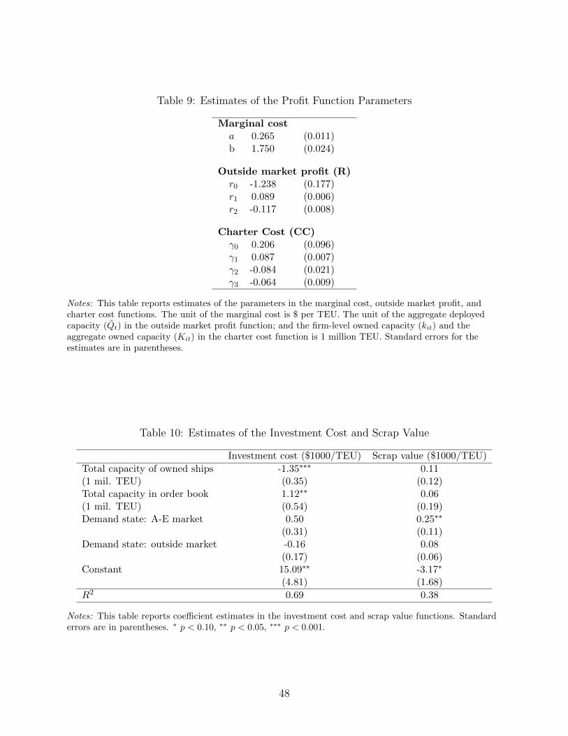
Table 9: Estimates of the Profit Function Parameters

Marginal costa 0.265 (0.011)b 1.750 (0.024)

Outside market profit (R)r0 -1.238 (0.177)r1 0.089 (0.006)r2 -0.117 (0.008)

Charter Cost (CC)γ0 0.206 (0.096)γ1 0.087 (0.007)γ2 -0.084 (0.021)γ3 -0.064 (0.009)

Notes: This table reports estimates of the parameters in the marginal cost, outside market profit, andcharter cost functions. The unit of the marginal cost is $ per TEU. The unit of the aggregate deployedcapacity (Qt) in the outside market profit function; and the firm-level owned capacity (kit) and theaggregate owned capacity (Kit) in the charter cost function is 1 million TEU. Standard errors for theestimates are in parentheses.

Table 10: Estimates of the Investment Cost and Scrap Value

Investment cost ($1000/TEU) Scrap value ($1000/TEU)

Total capacity of owned ships -1.35∗∗∗ 0.11(1 mil. TEU) (0.35) (0.12)Total capacity in order book 1.12∗∗ 0.06(1 mil. TEU) (0.54) (0.19)Demand state: A-E market 0.50 0.25∗∗

(0.31) (0.11)Demand state: outside market -0.16 0.08

(0.17) (0.06)Constant 15.09∗∗ -3.17∗

(4.81) (1.68)

R2 0.69 0.38

Notes: This table reports coefficient estimates in the investment cost and scrap value functions. Standarderrors are in parentheses. ∗ p < 0.10, ∗∗ p < 0.05, ∗∗∗ p < 0.001.

48

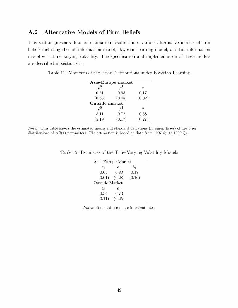
A.2 Alternative Models of Firm Beliefs

This section presents detailed estimation results under various alternative models of firm

beliefs including the full-information model, Bayesian learning model, and full-information

model with time-varying volatility. The specification and implementation of these models

are described in section 6.1.

Table 11: Moments of the Prior Distributions under Bayesian Learning

Asia-Europe marketρ0 ρ1 σ

0.51 0.95 0.17(0.63) (0.08) (0.02)

Outside marketρ0 ρ1 σ

8.11 0.72 0.68(5.19) (0.17) (0.27)

Notes: This table shows the estimated means and standard deviations (in parentheses) of the priordistributions of AR(1) parameters. The estimation is based on data from 1997:Q1 to 1999:Q4.

Table 12: Estimates of the Time-Varying Volatility Models

Asia-Europe Marketa0 a1 b1

0.05 0.83 0.17(0.01) (0.28) (0.16)

Outside Marketa0 a1

0.34 0.73(0.11) (0.25)

Notes: Standard errors are in parentheses.

49

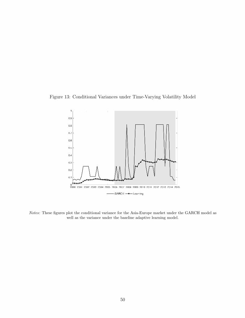
Figure 13: Conditional Variances under Time-Varying Volatility Model

Notes: These figures plot the conditional variance for the Asia-Europe market under the GARCH model aswell as the variance under the baseline adaptive learning model.

50

B Preliminary Evidence of Investment Policy Changes

Learning and full-information models make different predictions about firm behavior. A

learning model generally predicts that even after controlling for the state (which includes

all payoff-relevant variables), firms’ beliefs, hence firms’ actions will be different before and

after experiencing large demand shocks. By contrast, under full information firms’ perceived

probabilities of transitioning to different demand states from a given state stay fixed over

time as new demand realizations do not contain any new information. Therefore, I examine

whether firms’ investment behavior changes significantly after they experience large demand

shocks in order to search for indirect evidence of learning. In particular, I test for a structural

break in the firm’s investment policy function with an unknown break date following the

approach proposed by Andrews (1993) closely.

The structural break equation is given by

yit = β′1xitI(t < t) + β′2xitI(t ≥ t) + eit

where t is the break date, yit is new investment, and xit includes state variables. The state

variables include the demand states for the Asia-Europe market and the outside market; firm-

specific state variables including the owned capacity and the order book capacity; and the

industry state including the aggregate capacity of operator-owned ships and the aggregate

order book capacity.52

Instead of imposing an exogenous break date, I first pin down the break date by esti-

mating a structural break equation with different break dates and searching for the one that

maximizes the fit of the equation. A break date minimizes the sum of squared residuals

function defined as the following:

S(β, t) =∑t

∑i

(yit − β′1xitI(t < t)− β′2xitI(t ≥ t))2. (12)

The periods from 2007:Q2 to 2013:Q3 are considered as a break date because I need sufficient

observations before and after to estimate the equation. Figure 14 plots the sum of squared

residuals function for different break dates. The break date that minimizes the SSE is the

last quarter 2008, which coincides with the downturns in international trade.

Table 13 reports results for the estimation of the policy function with the last quarter

of 2008 as the break point as well as results from the structural break test. Based on the

test, I reject the null that the investment policy is the same before and after the last quarter

52The demand states are recovered through demand estimation as given in section 5.1.

51

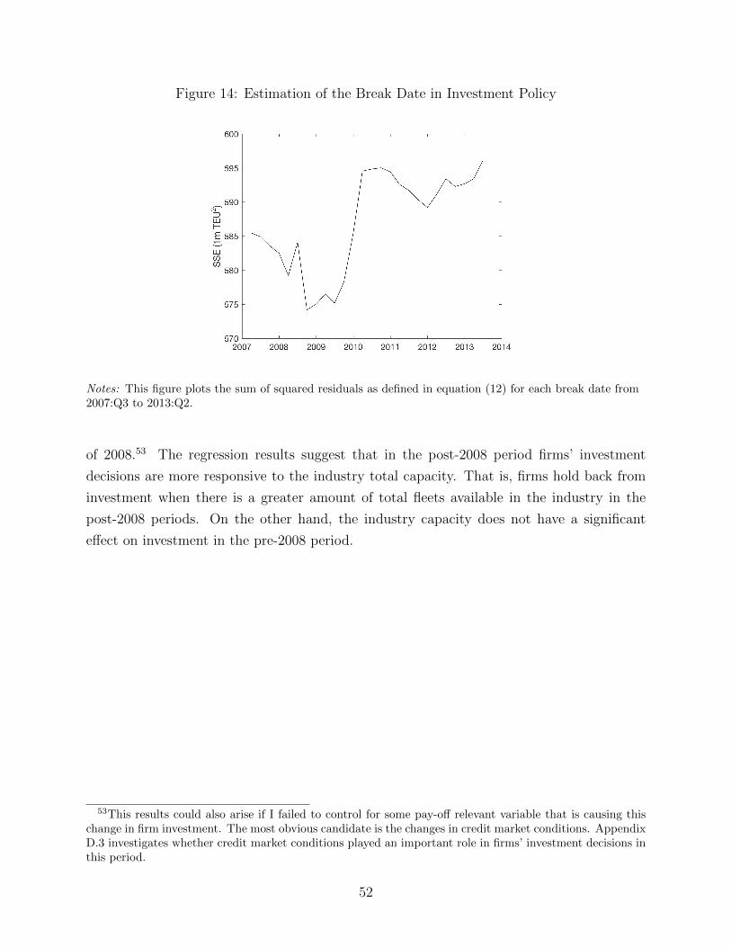
Figure 14: Estimation of the Break Date in Investment Policy

Notes: This figure plots the sum of squared residuals as defined in equation (12) for each break date from2007:Q3 to 2013:Q2.

of 2008.53 The regression results suggest that in the post-2008 period firms’ investment

decisions are more responsive to the industry total capacity. That is, firms hold back from

investment when there is a greater amount of total fleets available in the industry in the

post-2008 periods. On the other hand, the industry capacity does not have a significant

effect on investment in the pre-2008 period.

53This results could also arise if I failed to control for some pay-off relevant variable that is causing thischange in firm investment. The most obvious candidate is the changes in credit market conditions. AppendixD.3 investigates whether credit market conditions played an important role in firms’ investment decisions inthis period.

52

Table 13: Investment Policy Estimation and a Test of a Structural Break

Panel A: RegressionDependent variable: New investment (1000 TEU)t < 2008Q4

Constant -324∗∗ (151)Demand state (Asia to Europe) 22∗∗ (11)Demand state (Outside market) 6.7 (4.1)Owned ship capacity (1000 TEU) .037∗∗ (.014)Order book capacity (1000 TEU) -.029 (.022)Aggregate owned ship capacity (1000 TEU) .02 (.015)Aggregate order book capacity (1000 TEU) -.055∗∗ (.017)

t ≥ 2008Q4Constant 138∗∗ (66)Demand state (Asia to Europe) -4.4∗ (2.4)Demand state (outside market) .77 (1.3)Owned ship capacity (1000 TEU) .01 (.0075)Order book capacity (1000 TEU) -.0026 (.015)Aggregate owned ship capacity (1000 TEU) -.0097∗∗ (.0048)Aggregate order book capacity (1000 TEU) -.02∗∗ (.0069)

Observations 612R2 0.177

Panel B: Test of a Structural BreakH0 : β1 = β2

Test statistics 4.38p-value ( 0.0001)

Notes: Standard errors in parentheses. ∗ p < 0.10, ∗∗ p < 0.05, ∗∗∗ p < 0.001.

53

C Computation

To compute strategies under MME for the model described in 3.2, I adopt a computational

algorithm that is analogous to the standard value function iteration algorithm except for an

extra simulation step. Because the transition of the moment-based industry state s may not

be Markov, a simulation step is used to generate the Markov approximation of the transition

of this state. The algorithm starts with a choice-specific value function that maps from

the set of state-action pairs to values denoted as W η(µ, x, s). It contains expected values of

different actions prior to drawing random costs of investing and scrapping given beliefs about

demand η. Then, based on a simulation run in which firms play optimal strategies implied by

these choice-specific values, the algorithm constructs the perceived transition kernel Pµ[m′|s].The next step updates the values and strategies using the best response against the current

strategy and the perceived transitions kernel. Finally, equilibrium conditions are checked

based on the norm of the distance between the values in the memory and the updated

values. A more detailed description of the algorithm is provided as follows:

1. Initialize W η(µ, x, s) for all (µ, x, s) ∈ M × X × S, and optimal strategies, µ∗, that

W η implies.

2. Simulate a sample path of {st}Tt=1 for large T based on µ∗. Calculate the empirical

frequencies of industry state h(s) = 1TI{st = s} for all s ∈ S. Calculate the empirical

transition kernel as

Pµ[m′|s] =

∑Tt=1 I{st = s, mt+1 = m′}∑T

t=1 I{st = s}.

3. Calculate the new values for each state-action pair (µ, x, s) as:

W η(µ, x, s) = π(x, s)− ικ(s) + ν(δ, x)φ(s) + βEa,µ [V η(x′, s′|x, s)]

and obtain the new best response µ∗ = arg maxµW (µ, x, s|µ, µ∗) for all (x, s) ∈ X ×S.

4. Calculate the following norm: maxx,µ∑

ˆs∈S|W η(µ, x, s)−W η(µ, x, s)|h(s).

5. If the norm is greater than ε, update the values and the strategy profile with W and

µ∗ and repeat steps 2-5.

54

D Robustness

D.1 Adding a Dominant Firm’s State in the Moment-Based State

The moment-based Markov equilibrium as proposed by Ifrach & Weintraub (2016) allows

firms to keep track of the detailed state of dominant firms (strategically important firms)

as well as moments describing the state of fringe firms as their moment-based industry

state. In my application, firms’ industry states are further reduced to the the sum of states

of all firms However, MME strategies may not be optimal (i.e. there may be a profitable

unilateral deviation to a strategy that depends on more detailed information), if moments do

not summarize all payoff-relevant information. In order to investigate how robust equilibrium

strategies are to changes in the moment-based industry state, I consider a version in which

richer information is allowed in the industry state and compare model predictions and values

to the baseline case.

In particular, firms condition their strategy on the firm-specific state of the largest firm

(the dominant firm) in addition to the states in the baseline case including their own firm-

specific state, the sum of all firms’ states, and demand states. In one version, the dominant

firm’s capital, denoted as k1 is included in the information set and in the other version, the

dominant firm’s order book, b1. Let s′ denote the new industry state and let µ′ and V ′

denote the optimal strategy and the value of the new game based on s′ as the industry state.

The difference in the values of the baseline model and the model that includes the dominant

firm’s state for each underlying state s is defined as:

∆µ′(x, s) =V ′ηµ′,µ(x, s′)− V η

µ (x, s)

V ηµ (x, s)

.

The expected value of this deviation is computed as the weighted average through a simula-

tion where the weights come from simulations based on the baseline model, or V . Table 14

shows that model predictions stay robust when either of the dominant firm states is added.

The average difference in the values is not significantly different from zero for both cases.

D.2 Robustness Checks for the Adaptive Learning Model

As described in section 4, the adaptive learning model was implemented under the truncation

approach. This section presents results from the imputation approach in which imputed data

from 1966 to 1996 are used in the belief estimation. Figure 15 show the beliefs for the Asia-

Europe market for the adaptive learning model with λt = 0.02. The beliefs under the

55

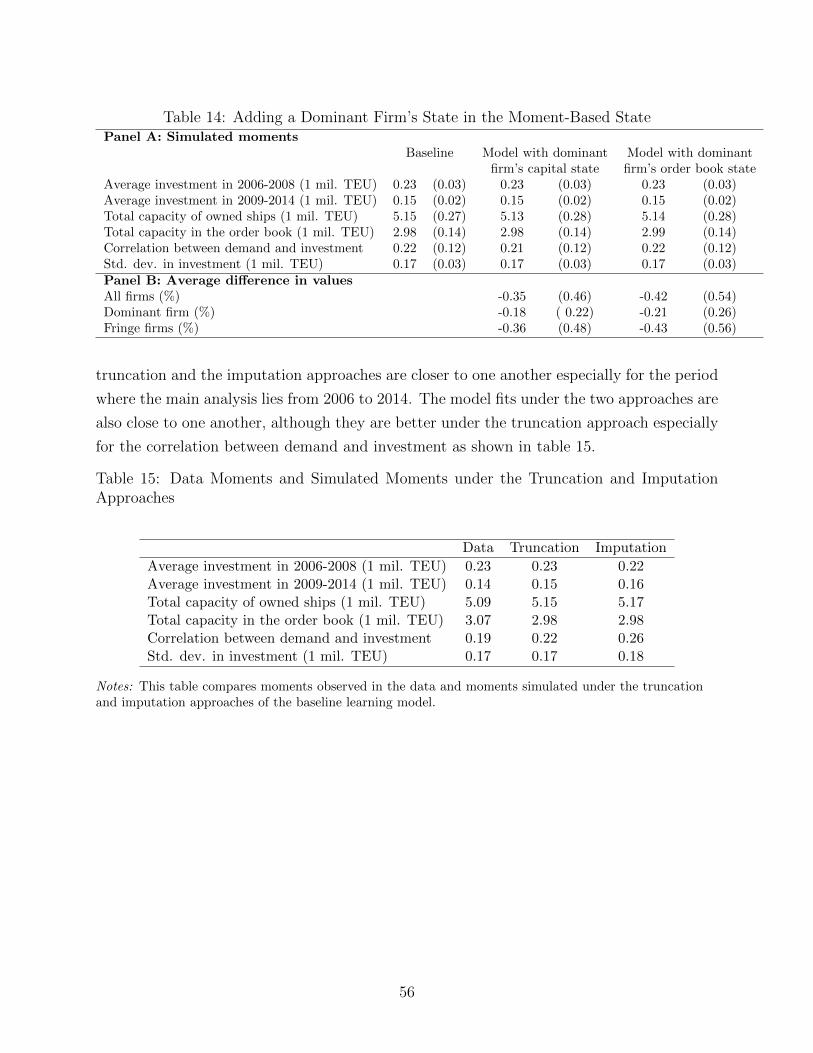
Table 14: Adding a Dominant Firm’s State in the Moment-Based StatePanel A: Simulated moments

Baseline Model with dominant Model with dominantfirm’s capital state firm’s order book state

Average investment in 2006-2008 (1 mil. TEU) 0.23 (0.03) 0.23 (0.03) 0.23 (0.03)Average investment in 2009-2014 (1 mil. TEU) 0.15 (0.02) 0.15 (0.02) 0.15 (0.02)Total capacity of owned ships (1 mil. TEU) 5.15 (0.27) 5.13 (0.28) 5.14 (0.28)Total capacity in the order book (1 mil. TEU) 2.98 (0.14) 2.98 (0.14) 2.99 (0.14)Correlation between demand and investment 0.22 (0.12) 0.21 (0.12) 0.22 (0.12)Std. dev. in investment (1 mil. TEU) 0.17 (0.03) 0.17 (0.03) 0.17 (0.03)Panel B: Average difference in valuesAll firms (%) -0.35 (0.46) -0.42 (0.54)Dominant firm (%) -0.18 ( 0.22) -0.21 (0.26)Fringe firms (%) -0.36 (0.48) -0.43 (0.56)

truncation and the imputation approaches are closer to one another especially for the period

where the main analysis lies from 2006 to 2014. The model fits under the two approaches are

also close to one another, although they are better under the truncation approach especially

for the correlation between demand and investment as shown in table 15.

Table 15: Data Moments and Simulated Moments under the Truncation and ImputationApproaches

Data Truncation Imputation

Average investment in 2006-2008 (1 mil. TEU) 0.23 0.23 0.22Average investment in 2009-2014 (1 mil. TEU) 0.14 0.15 0.16Total capacity of owned ships (1 mil. TEU) 5.09 5.15 5.17Total capacity in the order book (1 mil. TEU) 3.07 2.98 2.98Correlation between demand and investment 0.19 0.22 0.26Std. dev. in investment (1 mil. TEU) 0.17 0.17 0.18

Notes: This table compares moments observed in the data and moments simulated under the truncationand imputation approaches of the baseline learning model.

56

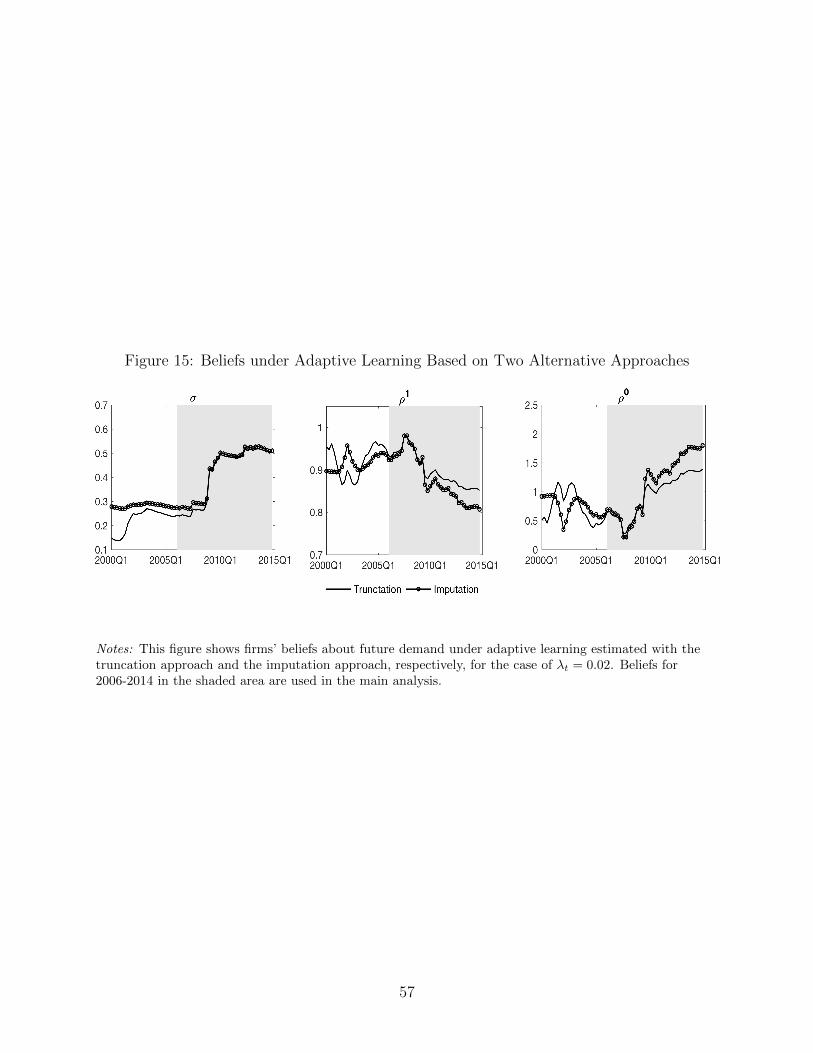
Figure 15: Beliefs under Adaptive Learning Based on Two Alternative Approaches

Notes: This figure shows firms’ beliefs about future demand under adaptive learning estimated with thetruncation approach and the imputation approach, respectively, for the case of λt = 0.02. Beliefs for2006-2014 in the shaded area are used in the main analysis.

57

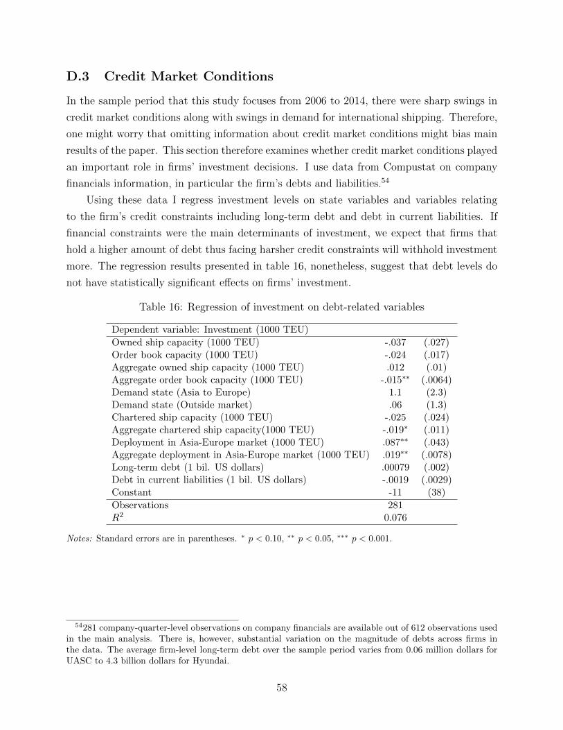
D.3 Credit Market Conditions

In the sample period that this study focuses from 2006 to 2014, there were sharp swings in

credit market conditions along with swings in demand for international shipping. Therefore,

one might worry that omitting information about credit market conditions might bias main

results of the paper. This section therefore examines whether credit market conditions played

an important role in firms’ investment decisions. I use data from Compustat on company

financials information, in particular the firm’s debts and liabilities.54

Using these data I regress investment levels on state variables and variables relating

to the firm’s credit constraints including long-term debt and debt in current liabilities. If

financial constraints were the main determinants of investment, we expect that firms that

hold a higher amount of debt thus facing harsher credit constraints will withhold investment

more. The regression results presented in table 16, nonetheless, suggest that debt levels do

not have statistically significant effects on firms’ investment.

Table 16: Regression of investment on debt-related variables

Dependent variable: Investment (1000 TEU)

Owned ship capacity (1000 TEU) -.037 (.027)Order book capacity (1000 TEU) -.024 (.017)Aggregate owned ship capacity (1000 TEU) .012 (.01)Aggregate order book capacity (1000 TEU) -.015∗∗ (.0064)Demand state (Asia to Europe) 1.1 (2.3)Demand state (Outside market) .06 (1.3)Chartered ship capacity (1000 TEU) -.025 (.024)Aggregate chartered ship capacity(1000 TEU) -.019∗ (.011)Deployment in Asia-Europe market (1000 TEU) .087∗∗ (.043)Aggregate deployment in Asia-Europe market (1000 TEU) .019∗∗ (.0078)Long-term debt (1 bil. US dollars) .00079 (.002)Debt in current liabilities (1 bil. US dollars) -.0019 (.0029)Constant -11 (38)

Observations 281R2 0.076

Notes: Standard errors are in parentheses. ∗ p < 0.10, ∗∗ p < 0.05, ∗∗∗ p < 0.001.

54281 company-quarter-level observations on company financials are available out of 612 observations usedin the main analysis. There is, however, substantial variation on the magnitude of debts across firms inthe data. The average firm-level long-term debt over the sample period varies from 0.06 million dollars forUASC to 4.3 billion dollars for Hyundai.

58