Embed Size (px)
Citation preview

DEMAND CURVE ESTIMATION
1

Demand curve estimation
• Statistical methods
− Problem: identification
− Examples: NY Mets, gasoline
• Surveys
• Experimenting
• Qualitative educated guessing
2

Demand curve estimation
• Statistical methods
• Surveys
− Eliciting truthful information
− Example: BBC
• Experimenting
• Qualitative educated guessing
3

Demand curve estimation
• Statistical methods
• Surveys
• Experimenting
− Can be very expensive (financially and reputationally)
− Examples: Amazon, Netflix
• Qualitative educated guessing
4

Demand curve estimation
• Statistical methods
• Surveys
• Experimenting
• Qualitative educated guessing
− See rules of thumb
5

Rules of thumb
• Rule of thumb 1: Demand for luxuries more sensitive to pricechanges than demand for necessities
− Food vs Armani suits
• Rule of thumb 2: Demand for specific products more sensitive toprice changes than demand for a category as a whole
• Rule of thumb 3: Long-run demand more sensitive to pricechanges than short-run demand
5

Rules of thumb
• Rule of thumb 1: Demand for luxuries more sensitive to pricechanges than demand for necessities
• Rule of thumb 2: Demand for specific products more sensitive toprice changes than demand for a category as a whole
− Mazda 323 vs cars overall
• Rule of thumb 3: Long-run demand more sensitive to pricechanges than short-run demand
5

Rules of thumb
• Rule of thumb 1: Demand for luxuries more sensitive to pricechanges than demand for necessities
• Rule of thumb 2: Demand for specific products more sensitive toprice changes than demand for a category as a whole
• Rule of thumb 3: Long-run demand more sensitive to pricechanges than short-run demand
− Gasoline
6

Statistical estimation
• From historical market data on quantity and price (q, p), estimatedemand as
ln q = α + β ln p + γ ln x + ξ
where x denotes demand shifters, ξ unobservables;parameters to estimate: α, γ and β (demand elasticity)
• β̂ < 0 for agricultural products, β̂ > 0 for industrial products!
7

The identification problem
p
q
S2
S1D3
D4
• • •
• • •
A BC
D EF
8

The identification problem
• If only demand shifts, data plots supply (e.g., ABC or DEF)
• If only supply shifts, data plots demand (e.g., AD, BE or CF)
• If both curves shift and if shocks are positively correlated(common occurrence) then data corresponds to DB or DC;connecting such points yields neither demand nor supply curve
• Key to identifying demand: find shocks that primarily shift supplycurve, not demand curve; more on this later
9

The endogeneity problem
• Suppose that price-setters observe demand shocks that statisticiandoes not; then p is positively correlated with ξ:
ξ = λ ln p + ε
where ε is unobserved by price-setters and statistician
• Then elasticity estimate is biased
ln q = α + (β + λ) ln p + γ ln x + ε
• If λ� 0, then will obtain positive estimate of demand elasticityeven though (as theory predicts) β < 0
10

Example: U.S. gasoline demand
11

Example: gasoline demand
50
100
150
200
250
300
350
110 120 130 140
p index (1983=100)
q index(1983=100)
19902000
2010
D1990
D2000 D2010
12

Example: gasoline demand
• Over time, increase in quantity and price
• Connecting dots implies positive “demand” elasticity!
• Possible solution: find controls x that shift demand: income,population, price of cars
• Expanded equation yields negative coefficient on ln p, but...
• Is this an unbiased estimate? Are there variables observable bymarket participants but not by me? Most likely
• Solution (as mentioned earlier): find shocks that primarily shiftsupply curve, not demand curve
13

US gasoline supply shocks and price
1.0
1.5
2.0
2.5
3.0
3.5
2003 2004 2005 2006 2007 2008
gasoline price US gasoline supply disruption
Time
price
supply disruption(Katrina)
300
600
900
1200
1500
14

US gasoline supply shocks and price
• Hurricane Katrina (2005) affected US gasoline supply considerably
• Arguably, effect on demand was small (drivers in southern LA)
• Supply shock implied higher price
• Estimate demand elasticity as ∆ log q/∆ log p for this period
• General procedure more complicated but same basic principle
• Var. “supply disruption” is called an instrumental variable
15

Example: demand for NY Mets tickets
16

Runs and dollars
Winning percentage # tickets/game
Year0.3
0.4
0.5
0.6
0.7
1992 1994 1996 1998 2000 2002 2004
??
10000
20000
30000
40000
tickets sold
winning percentage
Stars indicate seasons when the Mets made it to post-season play. Source: mbl.com
17

NY Mets performance at the ticket office
# tickets/game $ million
Year
......
......
......
......
......
......
......
......
......
......
......
......
......
......
......
......
......
......
......
......
......
......
......
......
......
......
......
......
......
......
......
......
......
......
....0
10000
20000
30000
40000
1992 1994 1996 1998 2000 2002 2004
50
100
tickets sold
season tickets
ticket revenues
? ?
Stars indicate seasons when the Mets made it to post-season play. A vertical dotted line indicates the introduction of variable pricing.Sources: baseball-almanac.com and New York Mets.
18

Demand for Mets tickets
10
20
30
10 20 30 40
p ($)
q (per game)(000)
1998
2000
D1998 D2000
19

Variable pricing
• Until 2002 season, prices uniform across games (not across seats)
• From 2003 season, four pricing tiers: gold, silver, bronze, value;later platinum as well
• Before season starts, games are classified in each tier; prices varyby a factor of 3 (gold/value)
20

Estimating demand elasticity
• Within year (until 2002) there is no price variation (across games)
• From year to year, price varies but so do unobservable demandshifters (e.g., fan’s expectations)
• After 2003, prices vary within season, but clearly endogenously
• Additional problem: capacity constraints and censored data
21

Shea Stadium (NY Mets)
22

Tickets sold per game: Mezanine Box
# tickets
Time0
1000
2000
3000
4000
1997 2000 2003
23

Tickets sold per game: Loge Box
# tickets
Time0
500
1000
1500
2000
2500
1997 2000 2003
24

Tickets sold per game: Upper Reserved
# tickets
Time0
5000
10000
15000
20000
1997 2000 2003
25
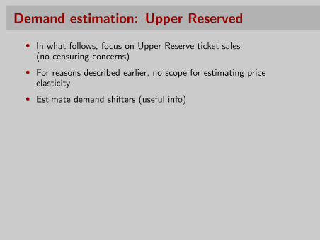
Demand estimation: Upper Reserved
• In what follows, focus on Upper Reserve ticket sales(no censuring concerns)
• For reasons described earlier, no scope for estimating priceelasticity
• Estimate demand shifters (useful info)
26

Upper Reserved
27

Upper Reserved ticket demand
Dummy variable Coefficient St. Dev. z p
Weekend 1078 402 2.68 0.01
Evening -905 391 -2.31 0.02
Season opener 8196 1373 5.97 0.00
July 2410 411 5.86 0.00
August 1425 415 3.43 0.00
September 1555 464 3.35 0.00
October 3774 1176 3.21 0.00
Yankees 9169 1002 9.15 0.00
Constant 401 634 2.21 0.03
28

Estimating price elasticity
• Quasi-natural experiment: in 2004 all tickets remained constantexcept Value Games in cheaper seats
• Use relative demand to account for cross-season effects
ε =log(r2) − log(r1)
log(5) − log(8)
where ri is attendance in cheap seats (price change) divided byattendance is more expensive seats (no price change)
• Based on this method (diff-diff), we obtain a demand elasticityestimate of approximately −.35
• What assumptions do we make to legitimize this approach?
29

Takeaways
• Empirically estimating consumer demand can be tricky
30