Embed Size (px)
Citation preview

The project “Development of smart and flexible freight wagons and facilities for improved transport of granular multimaterials” (HERMES) has received funding from the European Com-mission’s HORIZON 2020 Work Programme 2014 - 2015 “Smart, green and integrated transport”, topic MG.2.2-2014, under grant agreement no 636520
Deliverable D4.2
Validation of models
Development of smart and flexible freight wagons
and facilities for improved transport of granular
multimaterials


i
Deliverable Title D4.2 Validation of models
Related Work Package: WP4: Determine potential actions on the bulk freight that improve the
logistic operation (research activity)
Deliverable lead: LTU
Author(s): Simon Larsson (LTU), Pär Jonsén (LTU), Hans-Åke Häggblad (LTU), Gustaf
Gustafsson (LTU)
Contact for queries Pär Jonsén
Luleå tekniska universitet
971 87 Luleå
Sweden
T +46 (0) 920 49 34 60
Dissemination level: Public
Due submission date: 01/02/2016
Actual submission: 31/03/2016
Grant Agreement Number: 636520
Start date of the project: 01.05.2015
Duration of the project: 36 months
Website: www.hermes-h2020.eu
Abstract This document describes the experimental and numerical study of granu-
lar material flow. Experimental results are used to calibrate and validate
a constitutive model for granular material flow. A micro mechanical
model was used to model granite gravel flow.
Versioning and Contribution History
Version Date Modified by Modification reason
v.01 27/01/2016 Simon Larsson Initial draft
v.02 27/01/2016 Pär Jonsén Revision
v.03 28/01/2016 Hans-Åke Häggblad Revision
v.04 28/01/2016 Pär Jonsén Revision
v.05 01/02/2016 Ingrid Picas Revision
v.06 01/02/2016 Simon Larsson Revision
v.07 04/02/2016 Ingrid Picas Final version
v.08 18/03/2016 Simon Larsson Revision after request by PO
v.09 31/03/2016 Ingrid Picas Final version after revision request by PO

ii
Table of contents
Versioning and Contribution History .............................................................................................................. i
Executive Summary ....................................................................................................................................... 1
1 Introduction ........................................................................................................................................... 2
2 Experimental work for salt and potash .................................................................................................. 2
2.1 Materials ........................................................................................................................................ 2
2.2 Spreading of granular material on a plane surface ........................................................................ 3
2.2.1 Experimental setup and testing procedure 3
2.3 Silo flow experiment ...................................................................................................................... 5
2.3.1 Experimental setup and testing procedure 5
2.4 Experimental results ...................................................................................................................... 7
2.4.1 Spreading of granular material on a plane surface 7
2.4.2 Silo flow experiment 8
3 Simulation of salt and potash flow ......................................................................................................... 9
3.1 Constitutive model......................................................................................................................... 9
3.2 Assumptions and simplifications .................................................................................................... 9
3.3 Simulation of the spreading of granular materials on a horizontal surface ................................. 10
3.3.1 Model calibration – deposit profiles 10
3.4 Simulation of lab scale silo discharge ........................................................................................... 13
3.4.1 Flow pattern comparison 13
4 Numerical study of granite gravel flow ................................................................................................ 17
4.1 Study of abrasive wear during unloading of a tipper body .......................................................... 17
5 Discussion and conclusions .................................................................................................................. 19

1
Deliverable D4.2
Executive Summary
For granular material flow simulation a constitutive or micro mechanical model is required to obtain a
realistic behaviour. This document provides a description of the calibration of a constitutive model for
granular material flow at low pressures, and comparison with experimental results.
Two experimental lab scale studies of granular material flow were performed. Three granular materials
were studied. From the experimental studies information of the granular material flow behaviour in the
low pressure regime was obtained. Three different materials were tested: fine grained crystalline potash
(SMOP), coarse grained compacted potash (GMOP) and salt (NaCl). Results from the laboratory tests
could be used to calibrate a constitutive model for granular material flow. Granite gravel flow was mod-
elled with a micro mechanical discrete element method model.
For GMOP and SMOP a numerical calibration of material parameters valid in the low pressure regime was
carried out using the experimental results from the granular spreading on a plane surface experiment.
These calibrated parameters were then used to simulate the silo flow experiment, in order to compare
the numerical flow predictions against experimental results. For the simulation of GMOP, SMOP and salt
the smoothed particle hydrodynamics (SPH) method was used. For granite gravel a micro mechanical
discrete element method (DEM) model was used. The simulation of granite gravel flow is an ongoing
study but some useful initial results have been obtained. In a previous study the unloading of a tipper
body was performed and the abrasive wear from the flowing granite gravel was calculated. The results
from the granite gravel flow simulation are planned to be included in deliverable 4.3 in M12.
Numerical and experimental results are in good agreement. From this study, the previously obtained
triaxial data for higher pressures can be combined with the low pressure data to cover a wide range of
applications.
The study of wear on paint and steel is not fully evaluated at this stage. It is an ongoing work of HEM,
CTM and LTU in task 2.3, which is interconnected with WP4, and that is planned to be finalized in M18.
All other deliverables objectives have been achieved.

2
HERMES GA No. 636520
1 Introduction
To trust that the numerical model can reproduce real filling/discharge processes, comparison with exper-
imental results of the different material cases have to be performed. The flow of granular material can be
studied in lab scale in order to obtain experimental measurement data for validation of numerical model
results. Various granular materials have different flow characteristics and it is therefore important to be
confident that a numerical model can capture the actual flow characteristics. If the real flow behaviour
have been captured and characterised, the numerical flow prediction can be validated against the exper-
imentally measured flow behaviour. Granular flow for potash and salt can be simulated using the
smoothed particle hydrodynamics (SPH) method.
Granite gravel flow can be studied numerically with a discrete element method (DEM). To be confident
that the DEM simulations of granite gravel flow can be trusted the numerically calculated wear can be
compared to wear measured experimentally. An industrial application where this comparison can be
made is during the discharge of a tipper body loaded with granite gravel.
2 Experimental work for salt and potash
2.1 Materials
The experimental work was conducted on samples of the following granular materials: fine grained crys-
talline potash (SMOP), coarse grained compacted potash (GMOP) and fine-grained salt (sodium chloride).
The more fine-grained potash (SMOP) has a bulk density of 1.11 – 1.15 g/cm3, the angle of repose is 30°
and the particle size distribution is given in Table 1.
Table 1: Particle size distribution for the SMOP potash.
Tyler mesh mm Cumulative retained range (%)
16 1.0 7-21
28 0.600 30-55
48 0.300 66-90
65 0.212 80-96
100 0.150 85-97
150 0.106 89-98
>150 <0.106 100

3
Deliverable D4.2
The more coarse-grained potash (GMOP) has a bulk density of 1.00 – 1.05 g/cm3, the angle of repose is
35° and the particle size distribution is given in Table 2.
Table 2: Particle size distribution for the GMOP potash.
Tyler mesh mm Cumulative retained range (%)
4 4.75
5 4.00 4 maxi
6 3.35
8 2.36
9 2.00 78-86
10 1.70
12 1.40
16 1.00 99 min
32 0.50
>32 <0.50
Granite was used as gravel; the average density of granite is between 2.65 – 2.75 g/cm3.
2.2 Spreading of granular material on a plane surface
The scope of the experiment was to capture the slumping and spreading of granular material on a plane
surface. The granular material was initially at rest, confined within a cylinder. The cylinder was then re-
moved and the material is allowed to spread and settle under the influence of gravity. The shape of the
pile of granular material that formed when the material had settled was studied by image analysis. Using
image analysis the profile of the material could be extracted.
2.2.1 Experimental setup and testing procedure
The scope of the experiments was to study the flow behaviour and final disposition of a vertical homoge-
neous column of granular material when its confinement was removed. The three different materials
described in section 2.1 were tested.
In the experiment the confinement was a transparent cylinder with diameter D1 = 172 mm. The cylinder
was initially at rest at a horizontal wooden surface and was filled with granular material to a predefined
height H, 110 mm for GMOP, 105 mm for SMOP and 60 mm for salt. The cylinder was then quickly re-
moved via a pulley system, see Figure 1. A video camera filming at 240 frames per second was used to
capture the spreading of the granular material when the cylinder was released. In order to facilitate verti-
cal and upwards motion of the cylinder when it was removed, another cylinder with a slightly larger radi-
us was used as a guide for the smaller cylinder. The diameter of the larger cylinder D2 was 200 mm, see
Figure 1. The pulley system made it possible to have a quick removal of the cylinder, an important feature

4
HERMES GA No. 636520
if the granular material was to be considered as a homogeneous cylindrical pillar at release. When the
material was at rest at the horizontal surface the final deposit profile was extracted via image analysis,
see Figure 2. The image analysis was performed according to the following steps:
- The individual frames were exported from the video.
- The measurement scale was set by selection of a reference length in each frame. In this case
the diameter of the cylinder was used as reference length.
- A grid was superimposed to the frame to facilitate measurement of profile position.
- The coordinates of the end points of the lines in Figure 2 were used to create the final depos-
it profile.
Figure 1. Schematic of the experimental setup used for the granular spreading on plane surface experi-
ment.

5
Deliverable D4.2
Figure 2. Image analysis was used to determine the profile of the final deposit. The last frame from the
video sequence is used; the material is at complete rest at this point.
2.3 Silo flow experiment
The scope of the experiment was to capture the flow of granular material during the emptying of a flat
bottomed silo. The flow was initiated from an opening in the bottom of the silo. The emptying of the silo
was recorded with a video camera and with image analysis it was possible to extract the flow behaviour
at various instances of time during the flow.
2.3.1 Experimental setup and testing procedure
The silo was made of polycarbonate except for the front side which was made of transparent glass
through which the granular flow process was documented. Glass was used in order to avoid scratching
from the granular material, which could obstruct the image analysis. The emptying of the silo was carried
out though an opening in the bottom, Figure 4. The design allowed a quick release of the ratchet mecha-
nism.
The width of the opening could be varied in the range 25 – 100 mm. The depth of the silo could be varied
in steps with the possible depths: 50, 100, 150 and 200 mm. The following dimensions were used
throughout the experiments:
- Bottom opening width = 50 mm
- Silo depth = 200 mm
- Silo width = 200 mm
- Silo height = 400 mm
The experimental setup with GMOP as sample material is presented in Figure 3. A scale was placed be-
neath the silo, Figure 4, in order to study the mass flow rate. The silo was filled with granular material to a
fixed height. The granular material was then released through the gap in the bottom of the silo. The emp-
tying of granular material was documented using a video camera.

6
HERMES GA No. 636520
Figure 3. Experimental setup for study of
granular flow during the emptying of a silo.
Figure 4. Schematic of the mass flow study.
Figure 5. Illustration of the silo, top view.
Figure 6. Illustration of the silo, front view.
7
Deliverable D4.2
2.4 Experimental results
2.4.1 Spreading of granular material on a plane surface
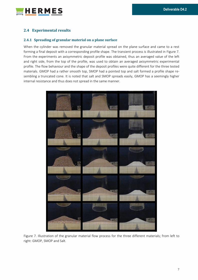
When the cylinder was removed the granular material spread on the plane surface and came to a rest
forming a final deposit with a corresponding profile shape. The transient process is illustrated in Figure 7.
From the experiments an axisymmetric deposit profile was obtained, thus an averaged value of the left
and right side, from the top of the profile, was used to obtain an averaged axisymmetric experimental
profile. The flow behaviour and the shape of the deposit profiles were quite different for the three tested
materials. GMOP had a rather smooth top, SMOP had a pointed top and salt formed a profile shape re-
sembling a truncated cone. It is noted that salt and SMOP spreads easily, GMOP has a seemingly higher
internal resistance and thus does not spread in the same manner.
Figure 7. Illustration of the granular material flow process for the three different materials; from left to
right: GMOP, SMOP and Salt.

8
HERMES GA No. 636520
2.4.2 Silo flow experiment
The angle that the material that remains in the silo after the emptying forms was measured, see Table 3.
GMOP had the largest value of this angle; SMOP had a lower value than GMOP but a larger value than for
salt. The angle of the remaining material in the silo increased with increased size of individual particles in
the granular materials.
Table 3. The experimentally measured angles that the granular material formed during the silo experi-
ment.
Material Angle, θ (acc. to Figure 8)
GMOP potash 41°
SMOP potash 36°
Salt 30°
Figure 8. Method used for determination of the
angle that the granular material forms at the end of
the silo flow experiment. This illustration shows the
angle for SMOP.
Figure 9. Illustration of the formation of a small hill
in the middle during the silo flow with salt as granu-
lar material.

9
Deliverable D4.2
3 Simulation of salt and potash flow
The experimental setup from the spreading of granular material on a plane surface was initially simulated
with the material parameters obtained from the previously performed triaxial tests (presented in deliver-
able 4.1). These parameters had to be rejected though, they resulted in a flow behaviour and shape and
position of the final deposit profile quite different from the experimental results. The cylinder model was
instead used for numerical calibration of a new set of material parameters, valid in the low pressure re-
gime.
The simulations of granular material flow for salt and potash were performed using the smoothed particle
hydrodynamics (SPH) method. SPH is a mesh-free Lagrangian particle method useful for simulation of
large deformations and local distortions where traditional methods, such as the finite element method
(FEM), have difficulties.
3.1 Constitutive model
The granular material was modelled using LS-DYNA constitutive model MAT_SOIL_AND_FOAM, which is
based on the work of Krieg (1972). The deviatoric perfectly plastic yield function φ is expressed in terms
of the second invariant of the deviatoric stress tensor
𝐽2 =1
2𝑠𝑖𝑗𝑠𝑖𝑗
pressure, p, and material constants a0, a1 and a2 as
𝜙 = 𝐽2 − [𝑎0 + 𝑎1𝑝 + 𝑎2𝑝2]
To explain the meaning of a deviatoric stress tensor it is noted that the stress tensor 𝜎𝑖𝑗 can be split in
two other tensors: one is the hydrostatic stress tensor which accounts for pure volume change of the
stressed body; the other is the deviatoric stress tensor 𝑠𝑖𝑗 which tends to distort the material, with no
accompanying volume change.
In addition to the yield function a load curve for pressure as a function of volumetric strain can be de-
fined.
3.2 Assumptions and simplifications
The material parameters obtained from the previously performed triaxial tests were considered not valid
in the low pressure regime. These material constants were found at high confining pressures and thus
can’t be directly used in a situation with low confining pressures, as is the case for both experiments pre-
sented in this work. Initial assumption that the material parameters obtained from the triaxial experi-
ments could be used in the low pressure regime proved false. Thus some further material parameter
calibration was necessary, in order to obtain material parameters valid in the low pressure regime. The
experiment studying spreading of granular material on a plane surface was selected for numerical mate-
rial parameter calibration. The parameters obtained from the numerical calibration are then used to sim-
ulate the experiments and to acquire a good agreement with the experimentally predicted material be-
haviour.

10
HERMES GA No. 636520
To facilitate the calibration of the material parameters in the constitutive model the material cohesion
was assumed to be zero for all three materials. The consequence of that assumption was that the materi-
al constants a0 and a1 could be put to zero. This leaves only one parameter for numerical calibration, a2.
The parameter a2 is related to the internal friction in the material, which is thought to be the governing
material parameter in the low pressure regime.
Some other necessary assumptions had to be made in order to perform the numerical calibration:
- Coefficients of static and dynamic friction were set to 0.6. It is noted that the effect of static
and dynamic friction was investigated where values between 0.1 – 1.2 did not have any signif-
icant effect on the end profile shape.
- No cohesion.
- Shear modulus and Poisson’s ratio from literature for sand. These parameters govern the
elastic response of the material, which is of lesser significance compared to the plastic behav-
iour as the material flows.
- Pressure was assumed to be a linear function of volumetric strain, using the bulk modulus,
corresponding to the shear modulus and Poisson’s ratio for sand, as slope. Thus no perma-
nent densification was allowed in the model. This was considered a valid approximation for
the low pressure regime, which was the region of interest in this study.
3.3 Simulation of the spreading of granular materials on a horizontal surface
The computational model is the spreading on a horizontal surface experiment, described in section 2.2.
The dimensions and initial filling heights are according to the experimental study. The granular material is
simulated using SPH with an axisymmetric formulation. FEM was used for the cylinder, which was consid-
ered rigid. Some simulation properties are presented in Table 4.
Table 4. Number of SPH nodes and computational time for simulation of spreading of granular material
on a horizontal surface.
Material No. of SPH nodes Comp. time
GMOP 9768 52 min
SMOP 9328 44 min
Salt 5368 18 min
3.3.1 Model calibration – deposit profiles
A calibration of the material model parameters was carried out using the experimental results from the
spreading of granular material experiment. The simulations were performed using axisymmetric repre-
sentations of the experiments described. For GMOP the initial aspect ratio of a=1.28 was used, corre-
sponding to initial height of 110 mm and initial radius of 86 mm. For SMOP the initial aspect ratio was
a=1.22, corresponding to initial height of 105 mm. For salt the initial aspect ratio was a=0.70, correspond-
ing to initial height of 60 mm. In Figure 10 - Figure 12 the experimentally measured profile is plotted to-
gether with the simulated profile. Both the left and the right side of the experimental profile is plotted, an
average of the both sides is also plotted. The numerical predictions correspond fairly well to the experi-

11
Deliverable D4.2
mental results, best perhaps for SMOP and GMOP. The calibrated material parameter a2 was found for
the three materials: GMOP a2=0.5, SMOP a2=0.4, salt a2=0.3.

12
HERMES GA No. 636520
Figure 10. GMOP, experimental results and simulat-
ed profile. Initial aspect ratio, a=1.28.
Figure 11. SMOP, experimental results and simu-
lated profile. Initial aspect ratio, a=1.22.
Figure 12. Salt, experimental results and simulated
profile. Initial aspect ratio, a=0.7.

13
Deliverable D4.2
3.4 Simulation of lab scale silo discharge
The computational model is the flat bottomed rectangular silo, described in Section 2.3. The dimensions
and filling height are set according to the experimental study. The simulation was performed using SPH
with a plane deformation formulation for the granular material. FEM was used for the silo walls that were
considered rigid.
Table 5. Number of SPH nodes and computational time for simulation of silo discharge.
Material No. of SPH nodes Comp. time
GMOP 40837 3h 24min
SMOP 30052 1h 30min
Salt 29245 1h 9min
3.4.1 Flow pattern comparison
A comparison between experimental results and simulated results was performed for GMOP, SMOP and
Salt. The simulated silo flow has a fairly good resemblance to the experimental results; see ¡Error! No se
encuentra el origen de la referencia. - ¡Error! No se encuentra el origen de la referencia.. Recall Figure 9
which illustrated the formation of a small hill in the middle during silo discharge with salt. This small hill
could be predicted in the numerical simulation of silo discharge with salt, see Figure 13.
Figure 13. The formation of a small hill in the middle during silo discharge with salt.

14
HERMES GA No. 636520
a)
b)
c)
d)
e)
f)
Figure 14. Comparison of experimental and simulated silo discharge with GMOP. The frames in a) and b)
represent time, t=0, c) and d) is at t=0.25 s, e) and f) is at the end of the discharge, at t=1.25 s.

15
Deliverable D4.2
a)
b)
c)
d)
e)
f)
Figure 15. Comparison of experimental and simulated silo discharge with SMOP. The frames in a) and b)
represent time, t=0, c) and d) is at t=0.25 s, e) and f) is at the end of the discharge, at t=1.25 s.

16
HERMES GA No. 636520
a) b)
c) c)
d) e)
Figure 16. Comparison of experimental and simulated silo discharge with salt. The frames in a) and b)
represent time, t=0, c) and d) is at t=0.25 s, e) and f) is at the end of the discharge, at t=1.25 s.

17
Deliverable D4.2
4 Numerical study of granite gravel flow
For granite gravel a micro mechanical discrete element method (DEM) model is used. With DEM the ma-
terial behaviour is determined by an alternation of Newton’s second law of motion and a force displace-
ment law at the contacts. The motion of each individual material particle from body and contact forces is
determined by Newton’s second law of motion. The force displacement law is used to update contact
forces arising from the relative motion of each contact. In the present study DEM is realized using rigid
spheres for each gravel particle. The interaction with other rigid or deformable structures is accomplished
with a penalty-based contact algorithm. The material behaviour is governed by normal and tangential
contact stiffness, contact damping coefficients and static and rolling friction coefficients. The micro mate-
rial parameters that were used for granite gravel are presented in Table 6.
Table 6: Micro mechanical material parameters for granite gravel.
Material Contact stiffness Contact damping Friction coefficients
Normal Tangential Normal Tangential Sliding Rolling
Granite gravel 0.3 0.01 0.98 0.98 0.6 0.1
4.1 Study of abrasive wear during unloading of a tipper body
Numerical simulation of granular flow with granite gravel has been carried out in another project at the
division of mechanics of solid materials at Luleå University of Technology. The simulation of granite gravel
flow is an ongoing study but some useful initial results have been obtained. In the previous study the
unloading of a tipper body was performed and the abrasive wear from the flowing granite gravel was
calculated, see Figure 17 - Figure 19.
Figure 17. Illustration of the load case. DEM repre-
sentation of the granite gravel.
Figure 18. Granite gravel flow during tipping.

18
HERMES GA No. 636520
Figure 19. Load intensity plot of the tipper loaded with granular material, [Forsström and Jonsén, 2014].

19
Deliverable D4.2
5 Discussion and conclusions
The two experimental setups described in section 2.2 and in section 2.3 were successfully used to study
granular material flow of GMOP, SMOP and salt. From the experimental studies information of the granu-
lar material flow behaviour in the low pressure regime was obtained. Granite gravel flow was modelled
with a micro mechanical discrete element method (DEM) model, described in section 4. Granite gravel
flow simulations using DEM was carried out in another project at the division of mechanics of solid mate-
rials at Luleå University of Technology. Some initial and promising results for simulation of granite gravel
flow and prediction of abrasive wear was obtained.
GMOP, SMOP and salt was simulated using smoothed particle hydrodynamics (SPH). Simulation of flow at
low pressures was initially attempted using the material parameters obtained from the triaxial tests. This
gave an unrealistic material response, not comparable to the experimental results. Thus it was concluded
that the material parameters obtained from triaxial tests were applicable only at high confining pressures,
similar to the conditions of the triaxial tests that were carried out at 30, 100 and 250 kPa confining pres-
sure. The small scale of the experiments conducted in this study resulted in low pressures in the granular
materials during testing. A numerical calibration of material parameter for low confining pressures was
carried out using the spreading of granular material on a horizontal surface experiment. The silo experi-
ment was used as a comparison between experimental and numerical flow prediction, where the materi-
al parameters from the numerical calibration were used. Material data obtained from the spreading of
granular material on a horizontal surface experiment is valid at the low pressure range. For higher pres-
sure the triaxial test data is already obtained for all material cases. To have a complete model that ranges
from low to high pressure a combination of the data can be done. This combined model is important for
studying the real filling and discharge processes as the pressure range will fluctuate with a larger range
that for the lab scale experiments presented here.
The simulated granular material flow was based on a very simple constitutive model. Assumptions were
made in order to facilitate the numerical parameter calibration. Thus the simulation of granular material
that was performed in this study has some limitations. The simple constitutive model can be viewed as a
very good start for further study of granular material flow. It is possible that in a future study some more
advanced material model will be used in order to correctly capture the flow behaviour at all confining
pressures.
Some suggestions for future improvements are listed:
- Accurate measurements of density at experimental conditions.
- Improve the experimental setup to make it possible to preload the granular material
enabeling testing at higher confining pressures.
- Perform additional triaxial tests in the low pressure regime.
- Include cohesion in the constitutive model and model the volumetric strain versus pressure
relationship according to experimental data.
- Use a more advanced constitutive model.