Embed Size (px)
Citation preview

Co-Extra – Deliverable D4.2 Co-Extra 007158
Page 1 of 72
CO-EXTRA
GM and non-GM supply chains: their CO-EXistence and TRAceability
Project number: 007158
Integrated project Sixth Framework Programme
Priority 5 Food Quality and Safety
Deliverable D4.2
Title: Procedure for the experimental design and validation of novel methods and guidelines for data processing, method validation and good data handling practices
Due date of deliverable: M18
Actual submission date: M33
Start date of the project: April 1st, 2005 Duration: 48 months
Organisation name of lead contractor: JRC
Revision: VFINAl
Project co-funded by the European Commission within the Sixth Framework Programme (2002-2006)
Dissemination Level
PU Public PP Restricted to other programme participants (including the Commission Services) PP
RE Restricted to a group specified by the consortium (including the Commission Services) CO Confidential, only for members of the consortium (including the Commission Services)
Co-Extra – Deliverable D4.2 Co-Extra 007158
Page 2 of 72
Task 4.2: Survey, analysis and development of guidelines and related statistical models for the
validation of novel methods
EU Co-Extra Task 4.2 Deliverable 4.2
Month 18 Final Report Edition co-ordinator: Malcolm Burns Authors: LGC: Malcolm Burns
Carole Foy Michael Griffiths
INRA: Valérie Ancel Andre Kobilinsky
GeneScan: Doerte Wulff Stefan Baeumler Anne Nemeth Andreas Wurz
JRC-IHCP: Gianni Bellocchi William Moens

Co-Extra – Deliverable D4.2 Co-Extra 007158
Page 3 of 72
1 Summary
This report describes preliminary findings associated with Task 4.2. These results are purely preliminary and describe developmental aspects associated with selected approaches for data analysis, and do not represent final working instructions, SOPs, standardised protocols, or fully validated statistical approaches, which are aspects which will be addressed as an additional deliverable associated with WP4 towards the end of the project. The aim of Task 4.2 was split into two main objectives: to develop preliminary guidelines for novel statistical models for experimental design and data analysis; and to develop preliminary guidelines for methods that do not fit into the standard scheme foreseen in the current guidelines for collaborative trials (e.g. multiplex methods and arrays). The first main section of this report addresses the aspect of data analysis in GM studies by exploring selected statistical approaches that are used in GM quantitation, and providing clearer explanations and outlining possible alternative models to implement. A commonly used technique in GM quantification is that of “absolute” real-time PCR, which relates the PCR signal to the actual amount of DNA using a calibration curve. Aspects of calibration curve construction using mean values and individual values; simple linear compared to weighted linear regression; alternative regression models; handling of duplex and singleplex results; transformation of data; comparison of regression curves; and handling of outlying values, were explored. These aspects can cause variability in the interpretation of results, and approaches to these must be standardised. Each of these aspects was examined, and novel statistical approaches suggested alongside guidelines on their applicability and implementation. Where possible, Microsoft® Excel files have been included to allow the implementation of these approaches. These preliminary guidelines will contribute towards a better understanding and help standardise methodologies involved in analysing data produced from trace detection situations, and should help towards comparison and standardisation of results. The quantitative PCR technique is further discussed as the bench-marking standard for use in GMO analysis. The model for absolute quantification is based on the production and use of a calibration curve. When this standard curve is generated, there is scope for errors to appear in the experimentation. The application of statistical approaches to this area facilitates the identification of errors and thus improves the quality of the results. Four situations were considered: test of normality, detection of outlying data points, test of linearity and comparison of regression curves. These user-friendly guidelines explain aims of each test and give examples of their use. Method validation is examined in further detail, and can be seen as the result of the composition of a variety of validation features. In addition to the basic approaches that are common to many laboratories, statistical and non-statistical (e.g. fuzzy rules) approaches are available to give analysts new insights that tailor the emphasis of the fit to the intended purpose of the method. For a general assessment of the method performance, the integration of all such partial features into a comprehensive methodology is required. Incorporation of analytical capabilities for method validation in today's laboratory practice by means of suitable software technology (AMPE is a supportive tool) would make method validation easy and practical, yet readable and exploitable by the whole scientific community. The second main section of this report addressed the topic of validation of multiplex real-time PCR methods for GMO analysis. Special aspects of the multiplex PCR situation compared to the simplex situation were introduced. Subsequently a detailed validation plan for a quantitative 'GMO-Reference-IPC' triplex is proposed including method parameters to be tested, experiments to be performed and acceptance criteria to be met. Special emphasis

Co-Extra – Deliverable D4.2 Co-Extra 007158
Page 4 of 72
has been set on method parameters specific to the multiplex situation. For these parameters additional explanations and recommendations are given. The third section of this report briefly outlines some of the current approaches that are used to evaluate the performance of microarrays. Creating reproducible data with a high level of consistency across array experiments and various platforms is widely accepted by the scientific community as a major problem. The complex nature of a microarray experiment results in many potential sources of variability, which can affect performance. This section reviews recent developments in the use of arrays for GMO detection, outlines the major sources of variability in the array process and discusses some of the approaches currently being used to evaluate performance and develop appropriate standards and controls to increase confidence in the measurements. The final section of this report summarises approaches and guidelines for the procedure for the validation of both current and novel methods.

Co-Extra – Deliverable D4.2 Co-Extra 007158
Page 5 of 72
CONTENTS
1 SUMMARY................................................................................................................................................... 3
2 PROCEDURES FOR DATA ANALYSIS.................................................................................................. 3
2.1 PROCEDURES FOR DATA HANDLING IN VALIDATION STUDIES ................................................................. 3 2.1.1 Introduction....................................................................................................................................... 3 2.1.2 Format of results ............................................................................................................................... 3 2.1.3 Calibration curve – averages vs. individuals .................................................................................... 3 2.1.4 Calibration curve – linear vs. weighted ............................................................................................ 3 2.1.5 Duplex and singleplex results............................................................................................................ 3 2.1.6 Arithmetic and geometric means ....................................................................................................... 3 2.1.7 Comparison of regression curves...................................................................................................... 3 2.1.8 Identification and handling of PCR outliers ..................................................................................... 3 2.1.9 References ......................................................................................................................................... 3
2.2 GUIDELINES FOR DETECTION OF OUTLIERS IN A LINEAR MODEL - APPLICATION FOR QUANTITATIVE
MODEL IN Q-PCR. ............................................................................................................................................... 3 2.2.1 Introduction....................................................................................................................................... 3 2.2.2 Introduction to R freeware ................................................................................................................ 3 2.2.3 How to use the file INRA-outliers.r ................................................................................................... 3 2.2.4 Description of functions .................................................................................................................... 3 2.2.5 Conclusion......................................................................................................................................... 3 2.2.6 References ......................................................................................................................................... 3
2.3 NOVEL APPROACHES TO METHOD VALIDATION - SOFTWARE AMPE ...................................................... 3 2.3.1 Introduction....................................................................................................................................... 3 2.3.2 Test statistics and numerical indices in method validation ............................................................... 3 2.3.3 Limitations of the current approach to method validation................................................................ 3 2.3.4 Fuzzy-based expert systems as an alternative approach to method validation ................................. 3 2.3.5 Software AMPE for use in method validation ................................................................................... 3 2.3.6 Remarks on method validation .......................................................................................................... 3 2.3.7 References ......................................................................................................................................... 3
3 GUIDELINES FOR THE VALIDATION OF QUANTITATIVE MULTIPLEX REAL-TIME PCR
SYSTEMS.............................................................................................................................................................. 3
3.1 INTRODUCTION....................................................................................................................................... 3 3.2 GUIDELINES FOR THE VALIDATION OF A QUANTITATIVE TRIPLEX 'GMO-REFERENCE-IPC' .................. 3
3.2.1 General.............................................................................................................................................. 3 3.2.2 General validation parameters for quantitative real-time assays for GMO analysis ....................... 3 3.2.3 Specific additional parameters for the Quantitative Triplex 'GMO-Reference-IPC' ........................ 3
3.3 VALIDATION PLAN FOR A QUANTITATIVE TRIPLEX 'GMO-REFERENCE-IPC'......................................... 3
4 REVIEW OF APPROACHES TO EVALUATE PERFORMANCE OF NOVEL METHODS ........... 3
4.1 BRIEF OVERVIEW OF MICROARRAY TECHNOLOGIES ............................................................................... 3 4.2 MICROARRAY PLATFORMS FOR GM ANALYSIS....................................................................................... 3 4.3 CRITICAL FACTORS AFFECTING PERFORMANCE OF MICROARRAYS ......................................................... 3 4.4 PERFORMANCE EVALUATION STRATEGIES.............................................................................................. 3 4.5 DEVELOPMENT OF REFERENCE MATERIALS AND STANDARDISATION INITIATIVES ................................ 3
4.5.1 External RNA Control Consortium ERCC ....................................................................................... 3 4.5.2 Microarray Quality Control (MAQC) Project .................................................................................. 3 4.5.3 Measurements for Biotechnology (MfB) Programme........................................................................ 3 4.5.4 The MGED Society............................................................................................................................ 3 4.5.5 ABRF Microarray research group (MARG) Research Group .......................................................... 3
4.6 CONCLUSION .......................................................................................................................................... 3 4.7 REFERENCES .......................................................................................................................................... 3
5 PROCEDURE FOR THE EXPERIMENTAL DESIGN AND VALIDATION OF NOVEL
METHODS ............................................................................................................................................................ 3
5.1 AIM ........................................................................................................................................................ 3

Co-Extra – Deliverable D4.2 Co-Extra 007158
Page 6 of 72
5.2 INTRODUCTION....................................................................................................................................... 3 5.3 CURRENT APPROACHES FOR METHOD VALIDATION ................................................................................ 3 5.4 PROCEDURES FOR THE VALIDATION OF NOVEL TECHNOLOGIES .............................................................. 3
5.4.1 Multiplex real-time PCR ................................................................................................................... 3 5.4.2 Microarrays....................................................................................................................................... 3 5.4.3 Macroarrays...................................................................................................................................... 3 5.4.4 Additional approaches to help in validation of novel technologies................................................... 3
5.5 SUMMARY .............................................................................................................................................. 3

Co-Extra – Deliverable D4.2 Co-Extra 007158
Page 7 of 72
List of Figures FIGURE 1. AMPLIFICATION PLOT FROM AN APPLIED BIOSYSTEMS 7700 REAL-TIME PCR SYSTEM.......................... 3
FIGURE 2. EXAMPLE CALIBRATION CURVE............................................................................................................... 3
FIGURE 3. CALIBRATION CURVE BASED ON MEANS FOR A RELATIVELY PRECISE DATA SET...................................... 3
FIGURE 4. CALIBRATION CURVE BASED ON INDIVIDUALS FOR A RELATIVELY PRECISE DATA SET. ........................... 3
FIGURE 5. CALIBRATION CURVE BASED ON MEANS FOR A RELATIVELY IMPRECISE DATA SET. ................................. 3
FIGURE 6. CALIBRATION CURVE BASED ON INDIVIDUALS FOR A RELATIVELY IMPRECISE DATA SET. ....................... 3
FIGURE 7. SINGLEPLEX CALIBRATION CURVE BASED ON MEANS OF THE CALIBRANTS. ............................................ 3
FIGURE 8. SINGLEPLEX CALIBRATION CURVE BASED ON SYSTEMATIC PAIR-WISE COMPARISONS............................. 3
FIGURE 9. NORMAL QUANTILE-QUANTILE PLOT ..................................................................................................... 3
FIGURE 10. GRAPH TO REPRESENT STANDARD CURVE ............................................................................................. 3
FIGURE 11. GRAPH TO SHOW TEST OF LINEARITY..................................................................................................... 3
FIGURE 12. GRAPH TO SHOW MULTIPLE REGRESSION LINES ..................................................................................... 3
FIGURE 13. STRUCTURE OF AN EXEMPLARY TWO-STAGE FUZZY-AGGREGATED VALIDATION INDICATOR. ............... 3
FIGURE 14. MEMBERSHIP TO THE FUZZY SETS. ........................................................................................................ 3
FIGURE 15. DIAGRAM REPRESENTING THE SOFTWARE AMPE. ................................................................................ 3
FIGURE 16. COMPETITION EFFECTS OF THE SPECIES SYSTEM ON THE GMO SYSTEM AGAINST SPECIES SYSTEM
PRIMER CONCENTRATION. ............................................................................................................................. 3
FIGURE 17. CROSS-TALK EFFECT OF HEX DYE (YELLOW) TO THE NEIGHBOUR CHANNELS FAM (GREEN), CY3
(ORANGE), ROX (RED), CY5 (DARK RED) ON TWO DIFFERENT QPCR PLATFORMS. ........................................ 3
FIGURE 18. STAGES INVOLVED IN A TYPICAL MICROARRAY EXPERIMENT................................................................ 3
FIGURE 19. DECISION TREE FOR THE PROCEDURE AND GUIDANCE ON VALIDATION OF NOVEL METHODS................. 3

Co-Extra – Deliverable D4.2 Co-Extra 007158
Page 8 of 72
List of Tables TABLE 1. MEANS AND STANDARD DEVIATIONS OF THE EXPERIMENTAL DATA SET .................................................. 3
TABLE 2. CT VALUES ASSOCIATED WITH A SAMPLE FROM A SIMULATED DATA SET. ................................................ 3
TABLE 3. SYSTEMATIC APPROACH FOR THE DETERMINATION OF THE GM CONTENT OF A SAMPLE. ......................... 3
TABLE 4. DIFFERENT REPLICATE COMPARISONS FOR THE DETERMINATION OF THE GM CONTENT OF A SAMPLE. .... 3
TABLE 5. EVALUATION OF THE GM CONTENT OF A SAMPLE BASED ON MEAN VALUES. ........................................... 3
TABLE 6. ARITHMETIC AND GEOMETRIC MEANS BASED ON A CLOSELY RELATED DATA SET. .................................. 3
TABLE 7. ARITHMETIC AND GEOMETRIC MEANS BASED ON A DIVERGENT DATA SET ............................................... 3
TABLE 8. VALUES OF CT.......................................................................................................................................... 3
TABLE 9. STANDARD CURVE VALUES ...................................................................................................................... 3
TABLE 10. DATA FOR TEST OF LINEARITY ................................................................................................................ 3
TABLE 11. DATA FOR COMPARISON OF REGRESSION CURVES................................................................................... 3
TABLE 12. SUMMARY OF STATISTICAL APPROACHES FOR METHOD VALIDATION IMPLEMENTED IN AMPE.............. 3
TABLE 13. MULTIPLEX ASSAY TYPES – SOME RELEVANT EXAMPLES. ..................................................................... 3

Co-Extra – Deliverable D4.2 Co-Extra 007158
Page 9 of 72
2 Procedures for data analysis
Contributor: Malcolm Burns - LGC
2.1 Procedures for data handling in validation studies
2.1.1 Introduction
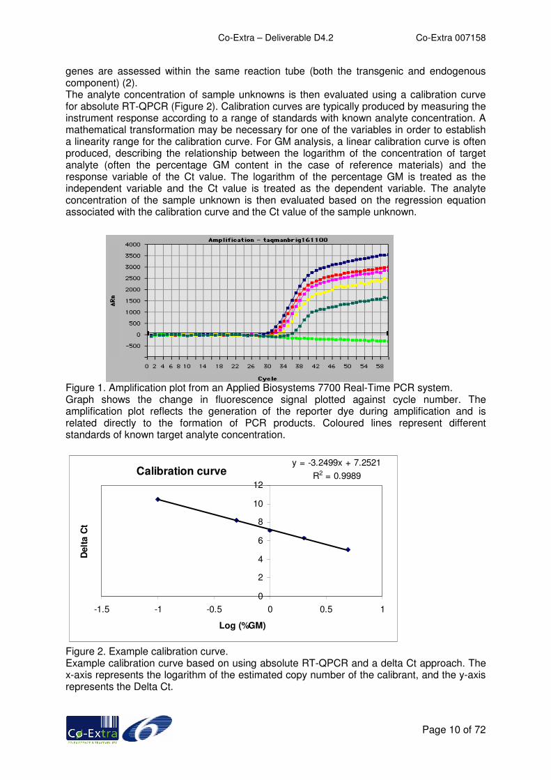
Accurate and precise determination of the concentration of an analyte at low levels is critically important in relation to identification and quantitation of genetically modified (GM) ingredients in food stuffs. The current “bench-marking” analytical technique for GM analysis is Real-Time Quantitative PCR (RT-QPCR), mainly due to the technique’s high quality performance characteristics such as sample throughput, precision and specificity. EC legislation (EC No 1830/2003) has established a de minimis threshold for the labelling of food and feed products of GM species as 0.9% of the ingredient which has been analytically translated in the total species component of a food product. The GM component can represent a low-level ingredient in a food product and it has to be determined whether the quantity of GM present in this portion is above or below this critical 0.9% level. It has however, to be mentioned that the unit (mass, DNA, kernels, etc.) to be used for calculating this percentage has not been specified and is thus still subject to controversy between seed companies and the International Seed Testing Association (ISTA) versus the food and feed supply chains stakeholders. In this report, the “unit” to be used for calculating the percentage is assumed to be a ratio of DNA contents ([GMO DNA copies number / GMO concerned species copies number] x 100). In RT-QPCR, gene specific PCR primers are used to amplify the targets of interest. Fluorescent probes, which are specific to particular DNA targets within the analyte, bind to the amplification products and are subsequently degraded by the enzyme Taq polymerase, resulting in a fluorescent signal. There is a net accumulation of a fluorescent response from the labelled probe over a set number of cyclical reactions, and this accumulation of fluorescent signal over time is proportional to the amount of PCR product formed, and hence the original amount of target analyte. Accurate quantitation is enabled by the accumulation of fluorescence signal above a background level where amplification is operating in an exponential manner prior to the impact of any inhibitory factors that cause the amplification to lose efficiency and plateau out (Figure 1). The cycle number where the target analyte signal crosses a pre-set threshold is referred to as the cycle threshold (Ct) value, and this value is directly proportional to the amount of target analyte in the sample DNA being analysed (1,2). The question as to what might be the best RT-QPCR approach for GM analysis has yet to be answered and be approved for universal satisfaction, hence the variety of approaches that are used. Aspects related to “absolute” RT-QPCR are focussed on in this section of the report. Absolute PCR relates the PCR signal to the actual amount of DNA target analyte by using a calibration curve. The reliability of this approach is dependent upon the assumption of equal PCR efficiencies between standards used and the sample unknown. For absolute RT-QPCR assays, two primers and probe sets are typically used. One set quantifies the amount of GM target present (transgenic probe), whilst another quantifies the total amount of starting material present from both the GM and non-GM material (endogenous probe). For absolute RT-QPCR using a delta Ct approach, the Ct value associated with the endogenous target is subtracted from the Ct associated with the transgenic target, as a normalisation step in order to take into account the original amount of total target analyte (i.e. GM plus non-GM soya). This resultant delta Ct value (Ct transgene minus Ct endogenous gene) is reported after the normalisation step. Assays can be conducted as a singleplex where only one target analyte (either transgenic or endogenous gene) is assessed per PCR reaction tube, or as a more complex duplex where both target
Co-Extra – Deliverable D4.2 Co-Extra 007158
Page 10 of 72
genes are assessed within the same reaction tube (both the transgenic and endogenous component) (2). The analyte concentration of sample unknowns is then evaluated using a calibration curve for absolute RT-QPCR (Figure 2). Calibration curves are typically produced by measuring the instrument response according to a range of standards with known analyte concentration. A mathematical transformation may be necessary for one of the variables in order to establish a linearity range for the calibration curve. For GM analysis, a linear calibration curve is often produced, describing the relationship between the logarithm of the concentration of target analyte (often the percentage GM content in the case of reference materials) and the response variable of the Ct value. The logarithm of the percentage GM is treated as the independent variable and the Ct value is treated as the dependent variable. The analyte concentration of the sample unknown is then evaluated based on the regression equation associated with the calibration curve and the Ct value of the sample unknown. Figure 1. Amplification plot from an Applied Biosystems 7700 Real-Time PCR system. Graph shows the change in fluorescence signal plotted against cycle number. The amplification plot reflects the generation of the reporter dye during amplification and is related directly to the formation of PCR products. Coloured lines represent different standards of known target analyte concentration.
Calibration curvey = -3.2499x + 7.2521
R2 = 0.9989
0
2
4
6
8
10
12
-1.5 -1 -0.5 0 0.5 1
Log (%GM)
Delt
a C
t
Figure 2. Example calibration curve. Example calibration curve based on using absolute RT-QPCR and a delta Ct approach. The x-axis represents the logarithm of the estimated copy number of the calibrant, and the y-axis represents the Delta Ct.

Co-Extra – Deliverable D4.2 Co-Extra 007158
Page 11 of 72
Some modern RT-QPCR platforms can facilitate the assessment of samples in 96 well and 384 well plate formats. These high throughput technologies can produce large volumes of data for subsequent analysis and interpretation. The complexity of many analytical assays and platforms often means that the best way to compare samples is not immediately obvious, and experimental designs that require normalisation and data transformation steps further complicate objective comparisons. The whole issue of the correct interpretation of data is further confounded by the fact that there are no standardised guidelines or protocols regarding data handling and reporting of results associated with GM identification and quantitation. Until such guidelines are in place, the confidence that can be attributed to a result will always be in doubt. This report addresses the above aspect of data analysis by exploring selected statistical approaches that are used in absolute RT-QPCR and GM quantitation, and providing clearer explanations and outlining possible alternative models to implement. These preliminary findings will contribute towards a better understanding and help standardise methodologies involved in analysing data produced from trace detection situations. This should help towards comparison and standardisation of results, and provide a set of “best practice guidelines”. Additionally, this report may also help for taking decisions both at the analytical laboratory and Competent Authorities level.
2.1.2 Format of results
This part of the report outlines six aspects of data analysis that can cause variability in the interpretation of results, and thus are candidates for providing guidelines for standardisation. Each aspect is introduced by stating what typical approaches are often used to facilitate the data analysis procedure. The next section introduces the novel statistical approach associated with the data analysis aspect of absolute RT-QPCR, and provides comments on its applicability and comparison with the more typical approaches. The final section suggests guidelines on how to facilitate and implement these novel statistical approaches, and where applicable Excel worksheets are provided on the EU Co-Extra website in order to implement these approaches.
2.1.3 Calibration curve – averages vs. individuals
2.1.3.1 Standard procedures
For GM quantitation using absolute RT-QPCR, a calibration curve is used to estimate the percentage GM content of the sample unknown. The value of the percentage GM content of the sample unknown is based upon the measured instrument response or a derivative of this (for example Delta Ct), and the equation relating to the calibration curve. The bias and precision associated with the calibration curve can affect the estimated value for the sample unknown, so calibrants which are known with high accuracy are needed. Certified Reference Materials (CRMs) provide suitable calibrants as these standards have been extensively characterised and their performance is certified with a given uncertainty estimate. The method is considered to be applicable over the working range of an instrument, and within this working range the linear range is defined as the range over which the method gives measured responses which are proportional to the concentration of the target analyte. For the estimation of the percentage GM content of sample unknowns, a simple linear regression model is typically used in order to fit the calibration curve. Simple linear regression is based on the method of least squares regression, which minimises the sum of the squares of the deviations between the observed and estimated values of the instrument response, given that a linear relationship exists.

Co-Extra – Deliverable D4.2 Co-Extra 007158
Page 12 of 72
2.1.3.2 Applicability of novel statistical approach and comparison with
standard validation procedures
Because of the high throughput capabilities afforded by many modern RT-QPCR machines, it is relatively easy to implement a sufficiently high replication factor associated with any sample (either as a calibrant or as a sample unknown). Simple linear regression can be conducted both on individual replicate values, and on the average values associated with a sample, and there are no standardised guidelines for the expression of the calibration curve related to GM quantitation experiments. Simulated data sets were used to explore the difference between applying simple linear regression to results based on the mean of calibrant groupings, and to the individual replicates of each calibrant. The simulated data sets were based on results from an Experimental data set, which was generated using a duplex RT-QPCR amplification technique (3). The Experimental data set consisted of nine replicate analysis plates each containing six replicates of five certified reference materials (CRMs) containing known amounts of GM soya per plate. The CRMs consisted of 0.1%, 0.5%, 1%, 2%, and 5% (w/w) Roundup Ready GM soya, obtained from the EU-IRMM (European Commission, Institute for Reference Materials and Measurements).
Amplification reactions (50µl) were performed with the TaqMan x2 Master Mix (Applied Biosystems, UK). Duplex reactions contained 50 nM endogenous primer Sltm1 and 900 nM endogenous primer Sltm2; 900 nM transgenic primers (LHRRfor and RHRRrev), 200nM of both the endogenous (Sltmp) probe and transgenic (TMPRR) probe. Reactions were run on the ABI Prism 7900 sequence detection system with the following thermal cycling protocol:
50°C for 2 mins, 95°C for 10 mins and 45 cycles of 95°C for 15 secs, 60°C for1 min. Data from all nine analysis plates was then pooled according to the five CRM groupings, with means and standard deviations as shown in Table 1. Each CRM grouping was tested for significant departure from a normal distribution and no significant differences were found (data not shown). This Experimental data set was used to model all other Simulated data sets described in this section.
CRM %GM value Mean Delta Ct Standard deviation of Mean Delta Ct
0.1 10.05 0.84 0.5 6.72 0.44 1 5.76 0.28 2 4.82 0.27 5 3.74 0.18
Table 1. Means and standard deviations of the Experimental data set The sample statistics were based on 45 replicates of each CRM. Delta Ct refers to the calculated difference in cycle threshold value (dependent variable) between probes targeting the transgene and the wild-type endogenous gene. A data set with relatively tight precision between replicates within the same calibrants was first examined – the average standard deviation within each calibrant grouping was 0.4 of a Ct. Figure 3 shows a calibration curve based on mean values and Figure 4 shows a calibration curve based on individual values, both applied to the same simulated data set.

Co-Extra – Deliverable D4.2 Co-Extra 007158
Page 13 of 72
Calibration based on meansy = -3.4684x + 5.7552
R2 = 0.9981
0
1
2
3
4
5
6
7
8
9
10
-1.5 -1 -0.5 0 0.5 1
Log (%GM)
De
lta
Ct
Figure 3. Calibration curve based on means for a relatively precise data set.
Calibration based on individualsy = -3.4684x + 5.7552
R2 = 0.9781
0
2
4
6
8
10
12
-1.5 -1 -0.5 0 0.5 1Log (%GM)
De
lta
Ct
Figure 4. Calibration curve based on individuals for a relatively precise data set.
The regression equation, and hence the regression statistics of the gradient and intercept, were identical for both calibration approaches. For this relatively precise data set, the correlation coefficient (r2) was slightly higher and better in the mean calibration approach (Figure 3), but is roughly equivalent to the individual calibration approach. However, as is typical with GM analysis, the precision associated with a group of calibrants can often depend upon the group’s mean value. Additionally, when looking at trace detection techniques, the precision associated with the calibrant representing a very low analyte concentration can be very poor. A simulated data set was thus used to represent an example of a GM experiment with relatively poor precision. Figure 5 shows a calibration curve based on mean values and Figure 6 shows a calibration curve based on individual values, both applied to the same relatively imprecise data set where each calibrant grouping had a standard deviation of 1 Ct.

Co-Extra – Deliverable D4.2 Co-Extra 007158
Page 14 of 72
Calibration based on meansy = -3.4421x + 5.5783
R2 = 0.9958
0
1
2
3
4
5
6
7
8
9
10
-1.5 -1 -0.5 0 0.5 1
Log (%GM)
Delt
a C
t
Figure 5. Calibration curve based on means for a relatively imprecise data set.
Calibration based on individualsy = -3.4421x + 5.5783
R2 = 0.6097
0
2
4
6
8
10
12
14
-1.5 -1 -0.5 0 0.5 1Log (%GM)
Delt
a C
t
Figure 6. Calibration curve based on individuals for a relatively imprecise data set.
The r2 value for the mean calibration approach was 0.9958, whilst the r2 using the individual calibration approach had a drastically reduced value of 0.6097. Thus, a data set with associated poor precision can give an apparently “good” result if the linear regression is simply applied to the average values and not the individual replicate values. The regression equation is the same irrespective of whether the calibration curve is produced using means or individual values, but the r2 value is representative of the total variability within the data set. For absolute RT-QPCR which utilises a calibration curve, it is recommended that calibration curves always be produced using replicate values from the entire data set, so that potential quality control issues within the data set can be identified immediately.
2.1.3.3 Guidelines on application of statistical approaches
Production of calibration curves for GM quantitation using individual values from the raw data is always advisable, as this will visually represent the spread of the data sets and also indicate any potential outlying values. The standard approach of using simple linear
Co-Extra – Deliverable D4.2 Co-Extra 007158
Page 15 of 72
regression typically plots just the mean values associated with each of the calibrants, and thus can give an uninformative correlation coefficient that does not represent the total variability of the calibrants. Application wise, standard computer spreadsheet software such as Microsoft Excel, can plot calibration curves displaying raw data values, so there is no need to purchase advanced statistical software packages. An Excel workbook which implements the construction of calibration curves using individual and mean values is available on the EU Co-Extra web space.
2.1.4 Calibration curve – linear vs. weighted
2.1.4.1 Standard procedures
For absolute RT-QPCR involving GM quantitation, the calibration curve facilitates estimation of the % GM content of sample unknowns, based on a derivative of the measured response from an analytical instrument. Typically, a simple linear regression line is used as the model to fit the calibration curve, and this is based on minimising the sum of squares of the deviates between the observed and expected response variable given a linear relationship exists. However, as is typical with many bio-analytical trace detection methodologies, and in particular those that are near the limit of detection, data sets often exhibit heteroscedastic behaviour. That is, the variance of a group of replicate calibrants is dependent upon that group’s mean value (2). For example, the precision with which the mean of the 0.1% CRM is known, is typically a lot poorer than the precision with which the 5% CRM is known. In these situations, the variance of each group of calibrants is inversely proportional to its mean value. In the cases where some calibrants are known with greater precision than others, the application of a simple linear regression model to the data set may not be sufficient to explain all of the variability in the data set (2).
2.1.4.2 Applicability of novel statistical approach and comparison with
standard validation procedures
Previous studies used a simulated data set that exhibited heteroscedasticity, which was then modelled using both linear and weighted regression. The weighted regression used a weighting of the inverse of the standard deviation for each calibrant group (2). Results showed that when the variance associated with each mean point of each calibrant group was roughly equivalent across the entire data set, the two regression approaches gave similar results (2). The most appropriate calibration curve must take into account the uncertainties and confidence intervals associated with the calibrant groupings. When there is dissimilar variance between the calibrant groupings, weighted regression is the most appropriate model to apply (2). The weighted regression model will predict slightly different results from the simple linear regression model, and as data is usually back transformed during the analysis, this has the potential to further inflate any differences between the two models (2). Additionally, the largest difference between the two regression approaches appears at the extremes of the linear ranges of the calibration curves where the weighting has the most influence. Furthermore, as GM quantitation experiments typically work with trace detection methods near or around the limit of detection, and current EU legislation requires the labelling of food products containing 0.9% GM or more on a weight by weight basis (EC regulation No 1830/2003), there is potential for these small differences between the calibration approaches to have critical effects upon the determination of the GM content of sample unknowns.
Co-Extra – Deliverable D4.2 Co-Extra 007158
Page 16 of 72
2.1.4.3 Guidelines on application of statistical approaches
Weighted linear regression should always be used when data sets exhibit heteroscedastic behaviour: when the variability associated with a data group is dependent upon the data group’s mean value. Most calibration curves associated with GM quantification use calibrants that often have a low target analyte concentration. These typically exhibit heteroscedastic behaviour where the lowest concentration of analyte has a relatively large variability, and the highest analyte concentration exhibits relatively tight precision. Statistically, weighted linear regression should be used on heteroscedastic data sets to ensure a more accurate answer than applying simple linear regression alone. In real terms, whether the weighted linear regression curve will give a significantly different response compared to the simple linear regression curve is dependent upon which region of the calibration curve is inspected, and also upon the data set used. Standard office based spreadsheets do not facilitate the application of weighted regression, and the user is advised to purchase statistical software packages such as Statistica (StatSoft Ltd.) or Minitab (Minitab Inc.), which will enable the application of different regression tools.
2.1.5 Duplex and singleplex results
2.1.5.1 Standard procedures
For the purposes of GM quantitation experiments, two probes are typically used. The transgenic probe is used to target the GM material, and an endogenous probe targets the total amount of plant species DNA represented by both GM and non-GM origins. In terms of absolute RT-QPCR, a delta Ct approach is often used for normalisation purposes. This Delta Ct value can be calculated based on the instrument response of the Ct value associated with the endogenous probe, subtracted from the Ct of the transgenic probe, for any given sample. For duplex reactions, the detection of the endogenous and transgenic targets are conducted within the same PCR well, whilst for singleplex reactions the two targets are in separate PCR wells.
2.1.5.2 Applicability of novel statistical approach and comparison with
standard validation procedures
Previous work (2) showed that bias can be introduced into the data analysis if any type of systematic approach is taken when comparing replicates of the transgenic and endogenous PCR reactions for the singleplex assay. This was based on the premise that there is no relationship between any given endogenous replicate with any other given transgenic replicate within singleplex reactions. It was suggested that a correct way to evaluate singleplex data sets is to take the mean of the endogenous replicates away from the mean of the transgenic replicates. The publication does not provide much insight into estimating standard deviations associated with singleplex results though, but refers the reader towards the rule of error propagation and then back-transforming the value into the units of the independent variable. The paper by Burns et al., 2004 described aspects related to the analysis and interpretation of data from real-time PCR trace detection methods using quantitation of GM soya as a model system (2). One of the aspects discussed related to the treatment of the evaluation of sample unknowns when using singleplex results. As there is no real relationship between any given replicate of an endogenous singleplex and any other replicate of a transgenic

Co-Extra – Deliverable D4.2 Co-Extra 007158
Page 17 of 72
replicate, bias can be introduced into the result if any systematic pair-wise comparisons are made. For example, Table 2 shows the data for a single sample whose GM content is unknown that has been assayed by a singleplex reaction and replicated three times for both the endogenous and transgenic probe. The Ct values associated with this sample were evaluated using two singleplex reactions of three replicates each. E1 to E3 are the replicate values based on the endogenous probe, and T1 to T3 are the replicate values based on the transgenic probe.
Endogenous Transgenic E1 E2 E3 T1 T2 T3
24.31 23.89 23.52 27.96 27.43 29.05 Table 2. Ct values associated with a sample from a simulated data set. Table 3 shows a systematic approach of taking the first replicate Ct value for the endogenous probe away from the first replicate Ct value for the transgenic probe, in order to evaluate the GM content of the sample. Calculations are based on taking the difference between similarly labelled replicates. The independent variable x is solved from construction of a calibration curve based on standards run with the sample unknown, using the regression equation of y = -3.6133x+6.0578 for this specific data set. %GM is calculated as the anti-log of x. The mean and standard deviation (sd) are calculated based on the three replicate comparisons.
Comparison Calculation X %GM Mean sd T1-E1 3.65 0.666 4.64 T2-E2 3.54 0.697 4.98 3.67 1.97 T3-E3 5.53 0.146 1.40
Table 3. Systematic approach for the determination of the GM content of a sample. However, there is no relationship between any given endogenous replicate with any other given transgenic replicate with singleplex reactions. As there is no relationship between T1-E1, the problem could be approached using different comparisons as detailed in Table 4. Calculations are based on taking the difference between differently labelled replicates. The independent variable x is solved from the equation y = -3.6133x+6.0578. %GM is calculated as the anti-log of x. The mean and standard deviation (sd) are calculated based on the three replicate comparisons.
Comparison Calculation X %GM Mean sd T1-E2 4.07 0.550 3.55 T2-E3 3.91 0.594 3.93 3.27 0.84 T3-E1 4.74 0.365 2.32
Table 4. Different replicate comparisons for the determination of the GM content of a sample. The means and standard deviations of the sample using the two approaches shown in Table 3 and Table 4 are very different. As there is no relationship between the replicates in a singleplex assay, both approaches are incorrect. If replicates of high endogenous and high transgenic values are always taken away from each other, significant bias can also be introduced. Statistically, the only correct way to evaluate the data set is to take the mean of the endogenous replicates away from the means of the transgenic replicates, as shown in Table 5. In Table 5 the calculations are based on taking the difference between the means of the transgenic and endogenous replicates. The independent variable x is solved from the equation y = -3.9181x+0.4411. %GM is calculated as the anti-log of x. The regression

Co-Extra – Deliverable D4.2 Co-Extra 007158
Page 18 of 72
equation is then solved for the independent variable, and anti-logs taken to calculate the %GM. This does not produce a standard deviation, but the calculation of this sample statistic is meaningless using the two former approaches.
Transgenic Mean
Endogenous Mean
Tm - Em X %GM
23.91 28.15 4.24 0.503 3.18 Table 5. Evaluation of the GM content of a sample based on mean values. In duplex assays, both the transgenic and the endogenous targets are amplified within the same reaction. Thus, there is a physical relationship between the two probes as they were subjected to the same PCR conditions. However, the same principle of interpreting the results applies: after subtraction, the mean of the duplex assays should be taken and then anti-logged to get the estimate of the %GM content of the sample. The paper concluded that care must be taken in this respect, as statistically the only correct way to evaluate a sample unknown based on a singleplex approach is to take the mean of the endogenous replicates away from the mean of the transgenic replicates instead of doing pair wise comparisons, and this would negate any potential bias in the results. Based on this conclusion, it would seem logical to apply these guidelines to the construction of a calibration curve based on singleplex data. Extending this same rationale to singleplex calibrants, we would intuitively suspect that making “pair-wise” comparisons of singleplex reactions can cause bias in results, and thus would affect the accuracy of the calibration curve. It would thus seem logical to base the calibration curve on the average results which have been computed by hand, based on the means of the singleplex results, in order to negate any potential bias. However, data handling strategies applied to calibration curves for singleplex data sets disprove this theory. All different pair wise comparisons were used for comparing endogenous and transgenic replicates together, for each CRM calibrant used for the production of the calibration curve, on a simulated data set for absolute RT-QPCR and GM quantitation. For single samples ([one replicate transgenic Ct] – [one replicate endogenous Ct]) this could give very different delta Ct values, as bias can be introduced dependent upon which replicates are compared to which. However, no matter how the individual replicates are compared or displayed on the graph, the calibration curve is exactly the same in terms of intercept and gradient (although different with the r2 value). As the individual points are used and displayed on the graph, why would the calibration curve be the same? This is because of the nature of the model that is being used to fit the data. Typically, simple linear regression analysis is used, and this is based on the estimation of the best fitting straight line that goes through the mean of each data group as this represents the minimum sum of squares of the residual variance. Thus, by the very act of applying the calibration curve, we are effectively taking the "mean" of a set of data points, and thus negating any potential bias we were getting from doing different pair-wise comparisons. The application of a simple linear regression to the same singleplex data set is illustrated in Figure 7 and Figure 8. Figure 7 is based on using the means of the singleplex calibrant groupings, and Figure 8 is based on using a systematic pair-wise comparison of neighbouring wells. This data set was based on a singleplex GM soya experiment that utilised five CRM calibrants for the construction of a calibration curve, where each calibrant was represented by three replicates.

Co-Extra – Deliverable D4.2 Co-Extra 007158
Page 19 of 72
Singleplex calibrants - Meansy = -3.8108x + 2.1152
R2 = 0.9947
-1
0
1
2
3
4
5
6
7
-1.5 -1 -0.5 0 0.5 1
Log (%GM)
Delt
a C
t
Figure 7. Singleplex calibration curve based on means of the calibrants.
Singleplex calibrants - systematic pair-wise y = -3.8108x + 2.1152
R2 = 0.959
-2
0
2
4
6
8
-1.5 -1 -0.5 0 0.5 1
Log (%GM)
Delt
a C
t
Figure 8. Singleplex calibration curve based on systematic pair-wise comparisons.
The conclusion to this is that it does not matter how the singleplex standards are treated with respect to data handling before the construction of the calibration curve. The standards can be compared via pair wise comparisons of neighbour with neighbour, pair wise comparison in systematic fashion, pair wise comparison in random fashion, or can be displayed simply as averages. By the very nature of applying a calibration curve to data, the line is forced through the mean values, so it does not matter how the data for singleplex calibration curves is displayed. Note that the correlation coefficient (r2) still varies between the mean approach (Figure 7) and the pair-wise approach (Figure 8) for the singleplex data set, which shows how much of the variability has been accounted for when using averages or individual values.
Co-Extra – Deliverable D4.2 Co-Extra 007158
Page 20 of 72
2.1.5.3 Guidelines on application of statistical approaches
When handling duplex data sets, the transgenic and endogenous reactions are present in the same well. If a delta Ct approach is to be taken, it is advisable to compute these based on individual wells and then to take an average of all these values. For singleplex data sets, significant bias can be introduced when comparing replicates of the transgenic and endogenous PCR reactions, dependent upon the comparisons made. In order to minimise any potential bias, it was suggested that the mean of the endogenous replicates is subtracted from the mean of the transgenic replicates. Application wise, the computation of both duplex and singleplex results using the above guidelines can easily be enabled using standard spreadsheet software such as Microsoft Excel.
2.1.6 Arithmetic and geometric means
2.1.6.1 Standard procedures
For the purposes of GM quantitation, calibration curves describe the relationship between the amount of target analyte and a response variable measured by an analytical instrument. The relationship between the response variable (often a Ct value for absoloute RT-QPCR) and the amount of target analyte is typically non-linear, and in order to elicit a linear response the amount of target analyte is often transformed using logarithm to base 10. Transforming the x-variable using logarithm base 10 helps normalise the data, and elicit a linear response between the x and y variables.
2.1.6.2 Applicability of novel statistical approach and comparison with
standard validation procedures
A question was posed in a previous publication (2) as to whether it was better to compute an arithmetic mean or a geometric mean for the evaluation of sample unknowns when back transforming the data. Simulated sets of data for GM detection analysis were used to evaluate the differences between the two approaches for interpreting the data. The generation of these simulated data sets are described in Section 2.1.3 “Calibration curve – averages vs. individuals”. In summary, this data set was generated using duplex RT-QPCR amplification technique for the quantitation of GM soya. The Experimental data set consisted of 45 replicates of five certified reference materials (CRMs) containing known amounts of GM soya per plate. The CRMs consisted of 0.1%, 0.5%, 1%, 2%, and 5% (w/w) Roundup Ready GM soya, obtained from the EU-IRMM (European Commission, Institute for Reference Materials and Measurements). Full experimental details can be found in (2). Table 1 shows the mean Ct and standard deviation associated with each of the CRMs from the Experimental data set. Delta Ct refers to the calculated difference in cycle threshold value between probes targeting the transgene and the wild-type endogenous gene. A simulated data set was based on the means and standard deviation of each CRM grouping from the Experimental data set, using six replicates of the five CRMs. The first approach to data evaluation used an arithmetic mean to evaluate the data. This involved taking anti-logs of all the individual data values, and then taking a mean. The second approach utilised a geometric mean to evaluate the data. This involved taking the mean of all the individual data values, and taking the anti-log of this mean value.
Co-Extra – Deliverable D4.2 Co-Extra 007158
Page 21 of 72
Data (x) Anti-log (x)
Arithmetic Mean
Mean of data
points
Geometric mean
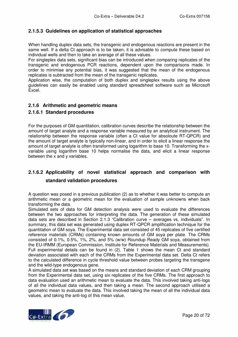
0.3 1.995 0.4 2.512 0.36 2.291 2.125 0.324 2.108 0.24 1.738 0.32 2.089
Table 6. Arithmetic and Geometric means based on a closely related data set. In Table 6, the logarithm of the percentage GM concentration of five sample replicate points is provided. The arithmetic mean is calculated as the mean of the five anti-logged data points. The geometric mean is calculated as the mean of the five data points, then taking the anti-log of this mean value. When individual data values are very similar, as in the above example, the arithmetic mean and geometric mean are very similar. Published literature suggests that the correct approach is to estimate the geometric mean. This approach reduces the effect of outlying data points, and is more representative of the results. Consider for example, where we have some outlying data points in another simulated data set:
Data (x) Anti-log (x)
Arithmetic Mean
Mean of data
points
Geometric Mean
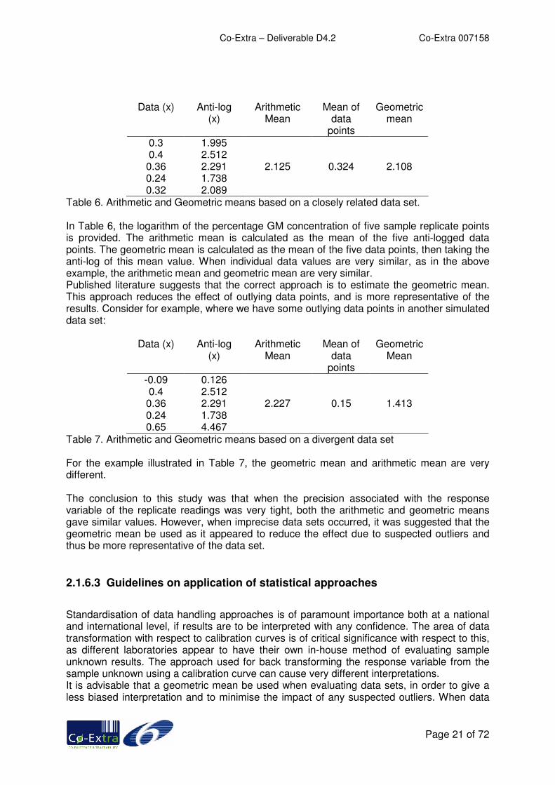
-0.09 0.126 0.4 2.512 0.36 2.291 2.227 0.15 1.413 0.24 1.738 0.65 4.467
Table 7. Arithmetic and Geometric means based on a divergent data set For the example illustrated in Table 7, the geometric mean and arithmetic mean are very different. The conclusion to this study was that when the precision associated with the response variable of the replicate readings was very tight, both the arithmetic and geometric means gave similar values. However, when imprecise data sets occurred, it was suggested that the geometric mean be used as it appeared to reduce the effect due to suspected outliers and thus be more representative of the data set.
2.1.6.3 Guidelines on application of statistical approaches
Standardisation of data handling approaches is of paramount importance both at a national and international level, if results are to be interpreted with any confidence. The area of data transformation with respect to calibration curves is of critical significance with respect to this, as different laboratories appear to have their own in-house method of evaluating sample unknown results. The approach used for back transforming the response variable from the sample unknown using a calibration curve can cause very different interpretations. It is advisable that a geometric mean be used when evaluating data sets, in order to give a less biased interpretation and to minimise the impact of any suspected outliers. When data

Co-Extra – Deliverable D4.2 Co-Extra 007158
Page 22 of 72
sets are relatively precise, both the arithmetic mean and the geometric mean will give similar results. The computation of either an arithmetic or geometric mean uses a simple and standardised approach to data handling, both of which can be easily facilitated using standard office spreadsheet software.
2.1.7 Comparison of regression curves
2.1.7.1 Standard procedures
There are a number of reasons why calibration curves are compared to each other in order to judge if they are performing to the same level of efficiency. These include testing if replicate runs of the same experiment are comparable, and also to test if the PCR efficiency between calibrants and sample unknowns is the same. Additionally, historical data sets may be compared to one another to determine if a reference material is still stable (4).
2.1.7.2 Applicability of novel statistical approach and comparison with
standard validation procedures
Until recently, the approach used to determine if calibration curves were behaving comparably was to examine the slope of the line and the correlation coefficient simply by visual inspection alone. This was a very subjective comparison, and it has been suggested that an objective approach using a simple derivation from the analysis of co-variance be used (4). This involves a statistical test to estimate the probability that the two regression lines were different simply due to chance alone. This test was explained in detail so that the calculations could be implemented in standard statistical software such as Microsoft Excel (4).
2.1.7.3 Guidelines on application of statistical approaches
The comparison of regression/calibration curves by visual inspection alone does not constitute an objective test. The application of the analysis of co-variance tool estimates a probability that the two regression curves are different due to chance alone, and thus overcomes the subjective element of comparisons. In all instances, an objective statistical tool such as the analysis of co-variance should be implemented. The application of the analysis of co-variance is not a standard option in many spreadsheet software packages. However, the analysis of co-variance tool uses a complicated but standardised approach, which can be written into software packages such as Excel. This worksheet is also available from the EU Co-Extra website.
2.1.8 Identification and handling of PCR outliers
2.1.8.1 Standard procedures
Inclusion of outlying values in a data set is liable to give rise to erroneous interpretations. Data arising from RT-QPCR must be treated carefully, as the artificially imposed end cycle number (maximum number of cycles) can preclude the application of some statistical tests for outliers as the data set can deviate substantially from a normal distribution. Additionally,

Co-Extra – Deliverable D4.2 Co-Extra 007158
Page 23 of 72
blank controls and other data points may lie near the maximum cycle number and further complicate efforts to identify outliers.
2.1.8.2 Applicability of novel statistical approach and comparison with
standard validation procedures
Published literature (4) described a simple visual approach using “box and whisker” plots as an aid to identifying potential outlying values. This visual plot utilised a non-parametric approach so that the data set did not have to follow a normal distribution. Data points that lay substantially beyond the 5 to 95% range of results were identified as potential outliers. This was followed by the application of a Grubb’s test (5) to objectively assess values to determine whether the data points were outliers, due to the Grubb’s test ease of application and computational simplicity. Throughout this procedure, ISO guidelines were followed to ensure that a consistent approach was taken for the identification and subsequent handling of statistical stragglers and outliers.
2.1.8.3 Guidelines on application of statistical approaches
An objective statistical approach for the identification of outliers is always advisable, and has been described previously (4), and is outlined below. Box and whisker plots can be used to help visually represent potential outlying data points. These plots can be applied using standard statistical software, such as Statistica (Statsoft Ltd). Typically, the “box” on the graph represents 50% of the data range based on the 1st quartile (25% confidence level) to the 3rd quartile (75% confidence level). The whiskers represent the 5 to 95% range of the results. Data points that lay substantially beyond this 5 to 95% range of results are classified as potential outliers. An outlier can be defined as a data point that does not follow the typical distribution of the rest of the data set and can be regarded as an irregular observation. This may be due to a number of reasons including the underlying distribution of the data set being non-normal in nature, operator error, a measurement mistake or transcription error, or purely due to chance alone. The Grubbs’ test (5) can be used to classify outliers, and is recommended by ISO 5725-2. The null hypothesis for the Grubbs’ test is that there are no outliers in the data set, whilst the alternative hypothesis is that there is at least one outlier present. The test statistic for the Grubbs’ test is computed from: Where: G = test statistic associated with Grubb’s test Yi = ith observation from data set / suspected outlier
Y = sample mean sd = standard deviation of data set The probability associated with the test statistic can be computed using formulae, but it is more common to determine the critical values associated with the test statistic using tables available in statistical publications (5). Based on ISO 5725 guidelines, outlying data points
G = max [ YYi − ]
sd

Co-Extra – Deliverable D4.2 Co-Extra 007158
Page 24 of 72
can be characterised according to the probability that their associated values can arise due to chance alone. Those values, which lie between 95% and 99% of the expected range of the characterised distribution, are termed stragglers (P value between 5% and 1%), and those values, which lie beyond 99% of the range of the characterised distribution, are termed outliers (P value below 1%). ISO 5725 recommends retention of stragglers in a data set unless there is a technical reason not to do so, based on the rationale that at the 95% level of confidence, there is a reasonable probability (5%) that the straggler could arise from the data set purely due to chance alone. For data points classified as outliers, ISO 5725 recommends rejection of the value before the subsequent data analysis, unless sufficient justification is given to retain it. This is based on the premise that there is an unacceptably high chance that the value does not belong to the rest of the data set. The application of this outlier test can be implemented using standard spreadsheet software and equations written in order to perform outlier testing such as the Grubb’s test, although the visualisation of the “box and whisker” plots may require more specialised statistical software. An Excel workbook which implements the approach described above for the identification of outlying values, is available on the EU Co-Extra web space.
2.1.9 References
1. “Comparison of plasmid and genomic DNA calibrants for the quantification of genetically modified ingredients” Burns M, Corbisier P, Wiseman G, Valdivia H, McDonald P, Bowler P, Ohara K, Schimmel H, Charels D, Damant A, Harris N. European Food Research and Technology (2006) 224(2): 249-258 2. “Analysis and interpretation of data from real-time PCR trace detection methods using quantitation of GM soya as a model system” Burns M, Valdivia H, Harris N (2004) Analytical and Bioanalytical Chemistry, 378(6): 1616-1623 3. “Event-specific detection of Roundup Ready Soya using two different real time PCR detection chemistries” Terry C, and Harris N (2001) European Food Research and Technology 213:425-431 4. “Standardisation of data from real-time quantitative PCR methods - evaluation of outliers and comparison of calibration curves” Burns M, Nixon G, Foy C, Harris N, BMC Biotechnology (2005) Dec 7, 5:31 doi: 10.1186/1472-6750-5-31 5. “Procedure for detecting outlying observations in samples”. Grubbs FE, Technometrics (1969), 11: 1-21

Co-Extra – Deliverable D4.2 Co-Extra 007158
Page 25 of 72
2.2 Guidelines for detection of outliers in a linear model -
Application for quantitative model in Q-PCR.
Contributors: Valérie Ancel; Andre Kobilinsky - INRA
2.2.1 Introduction
A definition given for an outlier 1 is an observation in a data set which is far removed in value from the others in the data set. It is an unusually large or an unusually small value compared to the others.
An outlier might be the result of an error in measurement, in which case it will distort the interpretation of the data, having undue influence on many summary statistics, for example, the mean.
An outlier is important because it might indicate an extreme of behaviour of the process under study. For this reason, all outliers must be examined carefully before embarking on any formal analysis. Outliers should not routinely be removed without further justification.
The whole document is based on results of Q-PCR experiments. The aim of statistical methods proposed below is to help the user with results interpretation. This document will describe 4 functions written in the language R, given in the file INRA-outliers.r available in the Co-Extra WP4 website, to detect outliers in 4 different cases.
• Normality of sample (function normality())
The normality hypothesis is often required to analyze a sample.
• Analysis of the linear model for quantitative model in Q-PCR
• Detection of outliers (function outliers())
This point could have a significance impact on the linear model estimation.
• Analysis of the linearity of the model (function linearity())
With small quantity or high quantity some problem could appear and the hypothesis of linearity would be reconsidered.
• Comparison of regression curves (function parallel())
With this tool, results of the same experiments can be compared.
Before describing in more details the content of the functions, some examples will be given. The interpretation of each example gives the aim of functions and the possibility to the user to understand how it is used. At first a short introduction to R is given with the name of the Web site to download it.
2.2.2 Introduction to R freeware
R is a free software environment for statistical computing and graphics. It compiles and runs on a wide variety of UNIX platforms, Windows and MacOS.
R provides a wide variety of statistical (linear and nonlinear modelling, classical statistical tests, time-series analysis, classification, clustering ...) and graphical techniques, and is highly extensible.
A version of a Setup program is available in the Web site:
http://cran.r-project.org/
1 available in the web site http://mathworld.wolfram.com
Co-Extra – Deliverable D4.2 Co-Extra 007158
Page 26 of 72
Many books or manuals explain the R language [6]. Several manuals are available in the web site mentioned. This document is based on the manual: W.N. Venables and D.M. Smith, An Introduction to R, 2004. It gives an introduction to the language and how to use R for doing statistical analysis and graphics.
2.2.3 How to use the file INRA-outliers.r
In this part, guidelines on how and when to use R program will be developed and an
application will be given for each functions.
2.2.3.1 The source() command
It is given with these guidelines a file, called "INRA-outliers.r", containing R functions (normality(), outliers(), linearity(), parallel()). To use these functions in R-program it is necessary to compile it. First of all, the source() command must be executed. > source('INRA-outliers.r')
Be careful, it is an obligation to indicate the way to access to the file "INRA-outliers.r". For windows a way as ’C:/Documents and Settings/MisterX/.../INRA-outliers.r’ is necessary. For UNIX or Linux it is possible to execute R in the folder wanted. Now R knows the names of the four functions and their operations. After that these functions could be used. To apply it, the user can just write the name of the function.
For these four functions a significance level has been fixed to 5% (value generally used to apply statistical test).
2.2.3.2 Normality testing
The aim of this function is to detect if observations follow a normal distribution. A normal distribution is often a reasonable model for the data. Without inspecting the data, however, it is risky to assume a normal distribution.
In this example, results of a Q-PCR experimentation are used. To test the homogeneity of a Q-PCR plate, the same sample has been put in each of the 96 wells. The results are in a file called "puit.txt" (not given here).

Co-Extra – Deliverable D4.2 Co-Extra 007158
Page 27 of 72
32.33816 32.61008 32.19653 32.25771 32.16341 31.38649 32.05720 31.69692 32.27598 32.25337 32.03976 31.98271 32.18341 32.05556 32.30661 32.05903 31.87684 32.21406 32.02682 32.24385 33.13905 32.13656 32.23290 32.26057 31.89561 32.38412 32.17732 32.09455 32.48780 32.27937 32.19342 32.14369 32.29722 32.11721 32.01817 32.34818 32.14246 32.02423 32.47526 32.17032 32.14277 32.01472 32.14271 31.87450 32.15717 32.14099 32.02337 32.09535 32.13511 32.24327 31.85132 31.59909 32.05164 32.17351 32.27779 32.18244 32.11783 31.84714 32.07211 32.08131 32.05851 32.03486 32.27569 32.28350 32.02474 32.25829 32.09168 32.33241 32.11679 32.72874 32.33609 31.79833 31.94181 32.51383 32.27136 32.21601 32.20788 32.00991 32.10532 32.36626 31.81827 32.08604 32.12590 32.03675 32.43835 32.23759 32.18463 32.28806 32.23347 32.12827 32.19744 31.77063 32.30376 32.11722 32.13732 32.00743
Table 8. Values of Ct
At first, the Table 8 "puit.txt" must be red by R. The R-function read.table() gives the possibility for reading a table in a file ".txt". As for the R-function source() it is necessary to indicate the way for windows. The command header=TRUE is used to indicate to R that the first line of the file contains the names of variables, in this example Ct. > tab<-read.table('puit.txt',header=TRUE)
Once the table containing the data is read by R, the name tab is given in R. To execute this function, only the vector containing Ct values is needed, vector called here tab$Ct. > normality(tab$Ct)
At first it draws the " Normal Quantile-Quantile Plot" as shown in Figure 9.
Figure 9. Normal Quantile-Quantile Plot
The straight line represents what our data would look like if it were perfectly normally distributed. Data are represented by the circles plotted along this line. Some points differ from the straight line and a first interpretation could let us to reject the hypothesis of normality for the data. To complete this analysis a Shapiro-Wilks test is performed.
Once Shapiro-Wilks test is done, the function gives an output with two possibilities:

Co-Extra – Deliverable D4.2 Co-Extra 007158
Page 28 of 72
• "Normality of the sample rejected with a level of 5% "
• "Normality of the sample accepted".
Here, the conclusion of the statistical test and the observation of the graphic is the rejection of the normality of the sample. Normality of the sample rejected with a level of 5%
If the hypothesis of normality is rejected, as shown above, an assumption of the presence of outliers in data can be expressed. So, tests for detecting outliers should be executed.
2.2.3.3 Detection of outlying data points
The aim of this function is to detect if a replicate differ from the rest of the replicates. A problem during the experimentation could appear and it is interesting to eliminate "bad" points before analyzing the data.
In this part, the test is realized from data of a standard curve. Four targets concentrations are tested with three replicates by concentration. The results of the Q-PCR are given in the file "1point.txt" (not given here).
Well Ct Quantity
H1
H2
H3
H4
H5
H6
H7
H8
H9
H10
H11
H12
30.63
30.82
30.83
28.59
28.67
29.11
26.19
26.29
26.34
24.00
23.71
23.68
50
50
50
200
200
200
800
800
800
3200
3200
3200
Table 9. Standard Curve values
The data are represented in Figure 10.
Co-Extra – Deliverable D4.2 Co-Extra 007158
Page 29 of 72
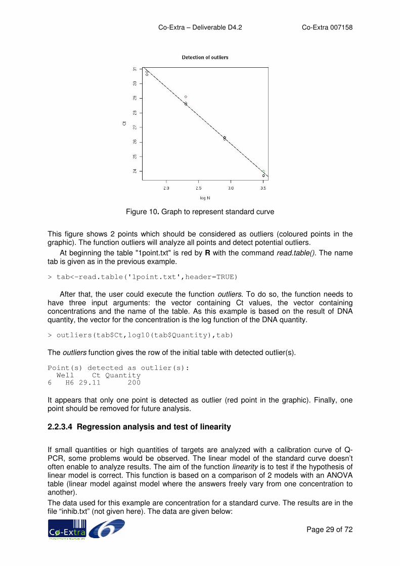
Figure 10. Graph to represent standard curve
This figure shows 2 points which should be considered as outliers (coloured points in the graphic). The function outliers will analyze all points and detect potential outliers.
At beginning the table "1point.txt" is red by R with the command read.table(). The name tab is given as in the previous example. > tab<-read.table('1point.txt',header=TRUE)
After that, the user could execute the function outliers. To do so, the function needs to have three input arguments: the vector containing Ct values, the vector containing concentrations and the name of the table. As this example is based on the result of DNA quantity, the vector for the concentration is the log function of the DNA quantity. > outliers(tab$Ct,log10(tab$Quantity),tab)
The outliers function gives the row of the initial table with detected outlier(s). Point(s) detected as outlier(s): Well Ct Quantity 6 H6 29.11 200
It appears that only one point is detected as outlier (red point in the graphic). Finally, one point should be removed for future analysis.
2.2.3.4 Regression analysis and test of linearity
If small quantities or high quantities of targets are analyzed with a calibration curve of Q-PCR, some problems would be observed. The linear model of the standard curve doesn’t often enable to analyze results. The aim of the function linearity is to test if the hypothesis of linear model is correct. This function is based on a comparison of 2 models with an ANOVA table (linear model against model where the answers freely vary from one concentration to another).
The data used for this example are concentration for a standard curve. The results are in the file “inhib.txt” (not given here). The data are given below:

Co-Extra – Deliverable D4.2 Co-Extra 007158
Page 30 of 72
Well Ct Quantity
G4 24.68 41777 G5 24.16 41777 G6 24.02 4177 G7 27.44 4177 G8 27.68 417 G9 27.47 417
Table 10. Data for test of linearity
At beginning Table 10 “inhib.txt” is red by R with the command read.table(). The name tab is given as in the previous examples. > tab<-read.table('inhib.txt',header=TRUE)
A first analysis of this curve gives a wrong efficiency (700%).
The data are represented in Figure 11.
Figure 11. Graph to show test of linearity
This figure clearly suggests that one point of dilution differs from the rest and it may be explained by a potential inhibition in data. The function linearity will analyze all points and tests the linearity of data, i.e. tests if a line is a good representation of the data. > linearity(tab$Ct,log10(tab$Quantity))
Once the comparison with ANOVA is done the function gives an output with two possibilities:
• "Linearity rejected with a level of 5% "
• "Linearity accepted".
Here, the conclusion of the test is the rejection of the linearity of the model. Linearity rejected with a level of 5%

Co-Extra – Deliverable D4.2 Co-Extra 007158
Page 31 of 72
The rejection of the hypothesis of linearity confirms the assumption of an inhibition in the PCR test.
A possible extension to this test is to give the point of dilution which differs from the rest. A multiple comparison procedure could be tested (but not given here).
2.2.3.5 Comparison of regression curves: test of diluted samples
A laboratory could for many reasons (criteria of repeatability ...) perform the same experiment and compare the results obtained. In this case a comparison between several calibration curves could be interesting. The function parallel will test if all curves could be considered as parallel lines, i.e. if the efficiency of each curve is the same.
In this example, the same standard curve is designed for many extracts from one GMO. Results are in Table 11 “parallel.txt”.
Ct Quantity Extract Ct Quantity Extract Ct Quantity Extract
32.83 50 1 32.50 200 4 29.95 800 7 33.06 50 1 32.14 200 4 29.52 800 7 31.68 200 1 29.41 800 4 33.47 50 8 31.46 200 1 29.08 800 4 33.26 50 8 29.32 800 1 31.51 50 5 31.47 200 8 29.38 800 1 32.09 50 5 31.53 200 8 35.94 50 2 30.36 200 5 28.93 800 8 35.82 50 2 30.64 200 5 28.72 800 8 33.04 200 2 28.37 800 5 32.56 50 9 32.64 200 2 28.42 800 5 32.67 50 9 30.34 800 2 34.20 50 6 30.53 200 9 30.04 800 2 33.81 50 6 31.09 200 9 32.76 50 3 32.69 200 6 29.35 800 9 33.10 50 3 33.10 200 6 29.19 800 9 31.49 200 3 29.74 800 6 32.86 50 10 31.91 200 3 29.91 800 6 33.03 50 10 29.62 800 3 33.27 50 7 30.84 200 10 29.93 800 3 34.04 50 7 31.23 200 10 33.34 50 4 32.03 200 7 28.10 800 10 33.63 50 4 32.52 200 7 28.11 800 10
Table 11. Data for comparison of regression curves
The table “inhib.txt” is red by R with the command read.table(). The name tab is given as in the previous examples. > tab<-read.table('parallel.txt',header=TRUE)
Data are represented in Figure 12.

Co-Extra – Deliverable D4.2 Co-Extra 007158
Page 32 of 72
Figure 12. Graph to show multiple regression lines
This figure shows two curves (in red) which differ from the others. A comparison with an ANOVA table is performed to explain this difference. > parallel(tab$Ct,log10(tab$Quantity),tab$Extract)
Once the comparison with ANOVA is done the function gives an output with two possibilities:
• "Test rejected with a level of 5% "
• "Test accepted".
Here, the conclusion of the test is the rejection of the hypothesis of parallel lines. Test rejected with a level of 5%
The rejection of the hypothesis of parallel lines gives an assumption for an extract effect. More analysis could complete this interpretation and give more proof of it (not done here [5]).
2.2.4 Description of functions
In order for to facilitate the use of R program a more details explanation of each command and the statistical method used is developed in the following pages.
2.2.4.1 Test of normality
The aim of this function is to detect if observations follow a normal distribution. The most useful tool for assessing normality is a quantile quantile or QQ plot. It is used to see if a given set of data follows some specified distribution (here a normal distribution). It should be approximately linear if the specified distribution is the correct model. Another method to test the normal distribution of data is to use the Shapiro-Wilks test [4].
2.2.4.1.1 Text to the programming language in R:
normality<-function(y) {
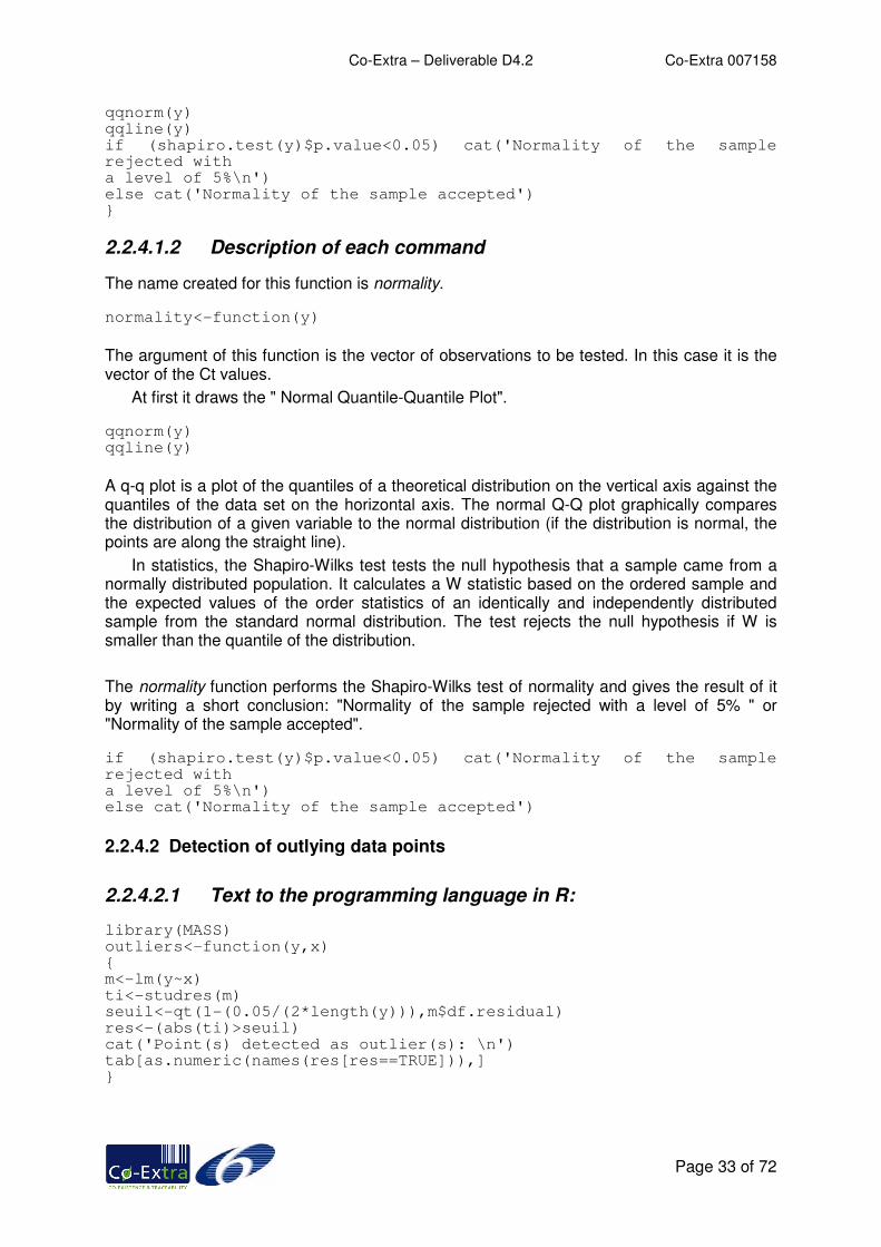
Co-Extra – Deliverable D4.2 Co-Extra 007158
Page 33 of 72
qqnorm(y) qqline(y) if (shapiro.test(y)$p.value<0.05) cat('Normality of the sample rejected with a level of 5%\n') else cat('Normality of the sample accepted') }
2.2.4.1.2 Description of each command
The name created for this function is normality. normality<-function(y)
The argument of this function is the vector of observations to be tested. In this case it is the vector of the Ct values.
At first it draws the " Normal Quantile-Quantile Plot". qqnorm(y) qqline(y)
A q-q plot is a plot of the quantiles of a theoretical distribution on the vertical axis against the quantiles of the data set on the horizontal axis. The normal Q-Q plot graphically compares the distribution of a given variable to the normal distribution (if the distribution is normal, the points are along the straight line).
In statistics, the Shapiro-Wilks test tests the null hypothesis that a sample came from a normally distributed population. It calculates a W statistic based on the ordered sample and the expected values of the order statistics of an identically and independently distributed sample from the standard normal distribution. The test rejects the null hypothesis if W is smaller than the quantile of the distribution.
The normality function performs the Shapiro-Wilks test of normality and gives the result of it by writing a short conclusion: "Normality of the sample rejected with a level of 5% " or "Normality of the sample accepted". if (shapiro.test(y)$p.value<0.05) cat('Normality of the sample rejected with a level of 5%\n') else cat('Normality of the sample accepted')
2.2.4.2 Detection of outlying data points
2.2.4.2.1 Text to the programming language in R:
library(MASS) outliers<-function(y,x) { m<-lm(y~x) ti<-studres(m) seuil<-qt(1-(0.05/(2*length(y))),m$df.residual) res<-(abs(ti)>seuil) cat('Point(s) detected as outlier(s): \n') tab[as.numeric(names(res[res==TRUE])),] }

Co-Extra – Deliverable D4.2 Co-Extra 007158
Page 34 of 72
If there are several repetitions for each concentration, the differences between their mean and each observation can be used to detect a possible aberration. In fact, we use Studentized residuals. Like standardized residuals, these are normalized to unit variance, but the Studentized version is fitted ignoring the current data point and allows to make a Student’s t-test [3]. The threshold adapted to perform this test is the chosen significance threshold of 5% divided by the number of observations. The aim of this division is to insure the global risk is below the initially defined threshold of 5%.
To execute this function the importation of the library MASS is needed. The R-function studres is located in it. library(MASS)
The name created for this function is outliers. outliers<-function(y,x,tab)
This function has 3 input arguments:
-y the vector which contains the observed data and called dependent variable
-x the vector of the fixed data called independent variable
-the name of the table containing data.
In our case the vector y contains the Ct values and the vector x contain the quantity fixed at the beginning of the experiment.
The R function lm() calculates the linear regression between x and y that is the slope and the intercept point of the curve. The R function studres() calculates Studentized residuals required to realize the statistical test. m<-lm(y~x) ti<-studres(m)
In this part we begin to calculate the threshold to compare with the statistic value. After that the test is performed and the function outliers gives the row of the initial table with the detected outlier(s). seuil<-qt(1-(0.05/(2*length(y))),m$df.residual) res<-(abs(ti)>seuil) cat('Point(s) detected as outlier(s): \n') tab[as.numeric(names(res[res==TRUE])),]
2.2.4.3 Regression analysis and test of linearity
2.2.4.3.1 Text to the programming language in R:
linearity<-function(y,x) { Quant<-as.factor(x) m<-lm(y~x) mq<-lm(y~Quant) if(anova(m,mq)$Pr[2]<0.05) cat('Linearity rejected with a level of 5% \n') else cat('Linearity accepeted \n') }
This function is based of a comparison of 2 models:

Co-Extra – Deliverable D4.2 Co-Extra 007158
Page 35 of 72
• Model A: a linear model with two parameters: the slope and the intercept point. The quality of the adjustment is measured by the residual sum of square of the deviation.
• Model B: model where the answers freely vary from one concentration to another. This model has one parameter by concentration tested.
We calculate the values of the parameters of the two models and we compare these two models with an ANOVA table based as usually on the residuals sum of square of the two models [5].
The name created for this function is linearity. linearity<-function(y,x)
This function has 2 input arguments: y is the dependent variable (vector which contain the observed data) and x the independent variable (the vector of the fixed data). In our case the vector y contains the Ct values and the vector x contain the quantity fixed at the beginning of the experiment.
To calculate the model B, where the answers (Ct) freely vary from one concentration to another one, a transformation of the values of independent variable is required. The R function factor is used to encode a vector as a factor. A factor of an experiment is a controlled independent variable, whose levels are set by the experimenter. So, there are as much levels as concentrations. Quant<-as.factor(x)
After creating a new variable (a factor), called Quant, the function calculates the 2 models. As in the function outliers, the R function lm is used. m<-lm(y~x) mq<-lm(y~Quant)
Once the 2 models are determined, the test for the comparison of the 2 models is realized with the R function anova. This (generic) function returns an object, which represents the analysis-of-variance tables. When given several objects, it tests the models against one another in the order specified. To conclude the p-value is analyzed. If the p-value is lower than the significance level (in this case 5%) the hypothesis of linearity is rejected, else it is accepted. if(anova(m,mq)$Pr[2]<0.05) cat('Linearity rejected with a level of 5% \n') else cat('Linearity accepted \n')
The function linearity gives the result by writing a short conclusion: "Linearity rejected with a level of 5% " or "Linearity accepted".
2.2.4.4 Comparison of regression curves: test of diluted samples
2.2.4.4.1 Text to the programming language in R:
parallel<-function(y,x,fac) { modalite<-as.factor(fac) m<-lm(y~x*modalite) mc<-lm(y~x+modalite-1) if (anova(mc,m)$Pr[2]<0.05) cat('Test rejected with a level of 5% \n')

Co-Extra – Deliverable D4.2 Co-Extra 007158
Page 36 of 72
else cat('Test accepted \n') }
This function is also based of a comparison of 2 models with an ANOVA table:
• Model A: model where the slopes and the intercepts associated to the different samples differ.
• Model B: model with a common slope for all sample and different intercept associated to the samples.
We calculate the values of the parameters of the two models and we compare these two models with an ANOVA table [5].
The name created for this function is parallel. parallel<-function(y,x,fac)
This function has 3 input arguments: y vector which contain the observed data (Ct values) and x the vector of the fixed data (Quantity) and fac which is a factor with many modalities (for instance: date, extract, sample ...).
As for the function linearity the variable of modalities must be transform like factor. For that the same R-function is used: modalite<-as.factor(fac)
After creating a new variable (a factor), called Quant, the function calculates the 2 models. As in the function outliers and linearity, the R function lm is used. m<-lm(y~x*modalite) mc<-lm(y~x+modalite-1)
Once the 2 models are determined, the test for the comparison of the 2 models is realized. The principle for the comparison of 2 models is similar to the function linearity. The model with only one slope for all samples is compared to the model with one curve for each model. If the test is rejected, the hypothesis of the parallel lines is rejected with a significance level of 5%. if (anova(mc,m)$Pr[2]<0.05) cat('Test rejected with a level of 5% \n') else cat('Test accepted \n')
2.2.5 Conclusion
The study of outlying data points is a preliminary step to analyze samples. An outlier could skew the interpretation of results, so its detection is important. This document describes 4 possibilities to detect outlying data points in a sample and gives a first approach to analyze results with the freeware R.
2.2.6 References
[1] Draper N.R. and Smith H. Applied regression analysis Second Edition. Wiley Series in Probability and Mathematical Statistics. New York: John Wiley, 1980.
[2] Faraway J.J. Practical Regression and ANOVA using R 2002.
Available in the Web site http://www.stat.lsa.umich.edu/ faraway/book
[3] Fox J. Regression diagnostics Sage University Paper series: Quantitative Applications in the Social Sciences, no 07-079. Newbury Park: Sage Publications, 1991.

Co-Extra – Deliverable D4.2 Co-Extra 007158
Page 37 of 72
[4] Royston P. A Remark on Algorithm AS 181: The W Test for Normality. Applied Statistics, 44, 547-551, 1995.
[5] Snedecor G.W. and Cochran W.G. Statistical methods Sixth Edition. Iowa State University Press, 1967.
[6] Venables W. N. and Ripley B. D. Modern Applied Statistics with S. Third Edition. New York: Springer, 1999.

Co-Extra – Deliverable D4.2 Co-Extra 007158
Page 38 of 72
2.3 Novel approaches to method validation - software AMPE
Contributors: Gianni Bellocchi; William Moens - JRC-IHCP
2.3.1 Introduction
There is a continuous and increasing need for reliable analytical methods to assess compliance with national and international requirements in all areas of analysis (1-4). The reliability of a method is determined by some form of validation, i.e. the procedure providing evidence of suitability of an analytical method for its intended purpose (5-6). Based on the results of a validation study, a method is considered or not as fit for the intended purposes. In most cases, formal validation requires the assessment of the performance of the proposed method by means of an inter-laboratory study (but see 7 for possible alternatives), also known as collaborative study or ring trial. Many national and international protocols defining criteria for the organization of these collaborative studies and interpretation of their results are available and routinely adopted. The International Standard Organization (ISO) (8) and the International Union for Pure and Applied Chemistry (IUPAC) (9-10) provide comprehensive standards describing various statistical procedures to assess analytical methods accuracy. The World Health Organization (WHO) (11) provides a detailed description regarding acceptance/rejection criteria for immunoassay kits and other protein binding systems. The Association of Official Analytical Chemists International (AOAC International, http://www.aoac.org) is a recognized worldwide authority on methods validation and quality analytical measurements. In the area of food quality and safety, the Codex Alimentarius Commission (12) requires the availability of specific performance information in order to include a method in the Codex commodity standard. In pharmacopoeia, the International Conference on Harmonisation (ICH) (13-14) and the United States Pharmacopoeia (USP) documents (15) are basic guidance for validation studies. According to available internationally standardized procedures, of which the examples mentioned above are only an extract, formal validation studies should provide detailed information regarding the conditions of method’s applicability and estimates for a series of validation measures, both necessary to assess overall method performance. This report provides a review of the interpretive results coming out of analytical methods validation studies commonly used in GM quantitation, and addresses novel approaches to summarize the information provided by individual validation indices and tests statistics into comprehensive indicators of method performance. Through the application of fuzzy logic (16), aggregated indicators are proposed as suitable tools for global evaluation of analytical methods, allowing also objective comparison across different methods. This will contribute towards a better understanding and harmonization of validation studies across different laboratories.
2.3.2 Test statistics and numerical indices in method validation
In agreement with international guidelines and protocols (e.g. 8-15), a collection of test statistics and numerical indices, from hereafter ‘validation metrics’, are routinely used to assess methods’ performance. Data check is commonly used to verify features such as normality of distributions, homogeneity of variances, and presence of anomalous data (stragglers, outliers). Some statistical tests (e.g. analysis of variance, linear regression analysis) are normally applied when one or more factors (or one or more regressors) are expected to affect the analytical response. Validation measures are used to provide information regarding a series of features which are internationally recognized as crucial for the overall evaluation of any analytical method performance, e.g. trueness, precision, specificity, detection limit, quantification limit, linearity, range. A brief description of the most

Co-Extra – Deliverable D4.2 Co-Extra 007158
Page 39 of 72
relevant ones follows, provided that an abundance of detailed documentation exists (e.g. 8, 11). Trueness: The departure of the average result of a method from a reference value. Precision: the closeness of agreement between independent results obtained under stipulated conditions (i.e. precision) is also evaluated and expressed in terms of standard deviation (or derived measures). Depending upon which factors (laboratory, analyst, instrument, time frame) are considered as possible sources of variation, three types of precision can be estimated: repeatability (all the factors are held constant), which provides information on the minimum variation intrinsic in a method; intermediate precision (one or more of the factors analyst, instrument or time frame are kept not constant); and reproducibility (the factor laboratory is also not kept constant), which provides information on the maximum variation that can be expected for a method. An assessment of methods by analyzing quantitatively the effects of deliberate and known variations in the operating conditions is known as robustness (or ruggedness). Quantification (or quantitation) limit: the smallest measured content above which a determination of the analyte is possible. In general, the limit of quantification of a method is associated with its limit of detection: the lowest concentration of analyte that can be detected, but not necessarily quantified, by the analytical method. Linearity: a method is required to elicit results that are directly, or by some mathematical transformation, proportional to the analyte concentration within a given range of application of the method. This is assessed via statistical analysis on correlation coefficient, y-intercept, slope, mean square error and lack of fit. Finally, specificity is the capacity of a method to respond exclusively to the analyte of interest.
2.3.3 Limitations of the current approach to method validation
A full validation study requires an extensive collaborative study to obtain the necessary data to assess the performance of a method and its transferability among laboratories. However, according to Muire-Sluis (17), analysts often point out that “validated methods may not be valid”. The question often arises: what exactly makes a validated method valid? According to the Center for Biologics Evaluation and Research (CBER) (18), “the acceptability of analytical data corresponds directly to the criteria used to validate the method”. This is a challenging issue because once a method is validated and estimates of the various validation metrics are available it is then up to the analyst to define an acceptance criterion on the basis of prior knowledge of the measurements as well as its intended application. For example, if the acceptance criterion is for a precision of 30%, all the methods showing precision lower than or equal to this threshold are acceptable. The acceptance criterion of a given validation statistic may not be easily defined by one threshold only, whereas two thresholds delimiting a ‘fuzzy’ area may be more suitable. As an example, the first threshold for variability measures such as repeatability (within-laboratory) or reproducibility (among laboratories) is the upper limit beyond which the method response is considered unacceptable; the second threshold is the lower limit below which the method is unquestionably good. Given the variability inherent to most laboratory instrument systems, the question whether a validation statistic is “good” or “bad” can be difficult to answer. In some cases, intuition, experience, knowledge of the practical context of the analytical data can be used to inspect or “eyeball” the data to assess a validation response. Most analysts would agree that very small or very large values of a validation metric determine a clear acceptance/rejection judgment. This issue was clearly exemplified in 19, where the authors indicated that a difference of 100% in a measurement typically exhibiting a precision of 1% is a real difference, and a difference of 0.01% is irrelevant for the same measurement. However, less clear-cut cases, which are very common in real-life situations, may be much more problematic for objective judgment and decision making. Another difficulty is linked to the fact that in some instances method’s reliability is assessed by means of one or few metrics, whether in other cases a more in-depth validation study may be required. When multiple metrics are used to assess methods’ performance (which is the most common case), organizing the data, processing the results and using them for an overall judgment might not be a trivial issue. In summary, validation studies as currently carried out have an intrinsic subjectivity linked to the interpretation of the

Co-Extra – Deliverable D4.2 Co-Extra 007158
Page 40 of 72
various metrics used, which are difficult to manage unless specific procedures improving objectiveness are introduced and adopted.
2.3.4 Fuzzy-based expert systems as an alternative approach to method validation
Each feature assessed via method validation (e.g. trueness, repeatability, reproducibility etc.) allows only a partial insight into the assessment of the overall method performance. In order to provide a solid and comprehensive quality judgment of an analytical method, the simultaneous joint evaluation of all the metrics is necessary. This is especially relevant when either some metrics are contradictory, that is when the performance of a method is satisfactory with respect to some features, but not with respect to others. In this respect combining multiple metrics into aggregated measures is useful in order to achieve a comprehensive assessment of the method’s response, to evaluate its performance in a variety of conditions (robustness/ruggedness testing), and to select the best method among several available with respect to specific needs. Despite the potential advantages, up to date there is no clear objective strategy to combine results from different metrics without being strongly affected by subjectivity. Indeed, personal preferences and specific needs may influence the interpretation of validation studies results. A strategy to improve objectivity is to weight the different metrics according to the intended use of the analytical procedure, and to summarize the information via aggregation of the weighted metrics. However, the strategy to aggregate them cannot merely rely upon summation, multiplication, or a combination of both (20). An effective approach to aggregate basic statistics can rely, instead, in setting up a fuzzy expert system using decision rules (16). This technique is robust on uncertain and imprecise data such as subjective judgments, and allows the aggregation of dissimilar metrics in a consistent and reproducible way (21). For these reasons, here we propose to summarize all the information collected during the validation study (independent metrics) via fuzzy logic, following the methodology described in 22. Fuzzy logic is derived from fuzzy group theory, dealing with reasoning that is approximate rather than precisely deduced from classical, or ‘crisp’, logic (23). Fuzzy logic uses predicates such as ‘good’-‘bad’, ‘high’-‘low’, or similar. Attaching a quality judgment to analytical methods, such as ‘accurate’-‘inaccurate’ or ‘precise’-‘imprecise’ follows as a consequence of validation (e.g. 24). According to ‘crisp’ group assumption, an element can only be or not in a group: if, for instance, a sub-group consists of the methods with at least 30% of precision (maximum acceptable standard deviation over the mean), a particular method can be classified as a member or not a member of the sub-group. If, however, a method is defined to be the sub-group of ‘precise’ methods, then it is more difficult to determine if a specific method is in the sub-group. If one decides that only methods with a minimum precision of 30% are in the sub-group, then a method with precision of 30.1% cannot easily be classified as ‘imprecise’ even though it is ‘almost imprecise’. The use of fuzzy group theory is compelling because available threshold values for precision and other relevant validation metrics are often vague and/or uncertain. Thus classification based on an abrupt transition between groups is doubtful. Fuzzy group theory addresses this type of problem by allowing one to define the ‘degree of membership’ of an element in a group by means of a membership function. For ‘crisp’ groups, the membership function only takes two values: 0 (non-membership) and 1 (membership). In fuzzy groups the membership function can take any value from the interval [0, 1]. The value 0 represents complete non-membership, the value 1 represents complete membership, and values in between (transition interval) are used to represent partial membership. The example in Figure 13 illustrates the implementation of fuzzy logic: first six metrics estimated in a method validation (correlation coefficient, t-test probability of intercept=0, t-test probability of slope=1, percent bias, percent repeatability standard deviation, percent reproducibility standard deviation) are transformed into fuzzy modules (linearity, trueness, precision) and, second, the three modules are aggregated into a synthetic indicator.

Co-Extra – Deliverable D4.2 Co-Extra 007158
Page 41 of 72
membership
function
S[x; a = min
(F, U); b
=max (F, U)]
bias (B, %)
F Partial U
≤ 15 ↔ ≥ 30
F
U
repeatability (RSDr, %)
F Partial U
≤ 10 ↔ ≥ 30
validation indicator
membership
function
S[x; a = 0; b = 1]
linearity
F Partial U
0 ↔ 1
trueness
F Partial U
0 ↔ 1
Expert
weight
F F F
F F U
F U F
F U U
U F F
U F U
U U F
U U U
precision
F Partial U
0 ↔ 1
validation modules
reproducibility (RSDR, %)
F Partial U
≤ 15 ↔ ≥ 50
F F
F U
U F
U U
0.00
1.00
0.00
0.50
0.50
1.00
0.00
0.30
0.15
0.45
0.55
0.85
0.70
1.00
corr. coeff. (r, %)
F Partial U
≥ 0.99 ↔ ≤ 0.90
intercept (p(t)_b0)
F Partial U
≥ 0.05 ↔ ≤ 0.01
slope (p(t)_b1)
F Partial U
≥ 0.05 ↔ ≤ 0.01
F F F F F U
F U F
F U U
U F F
U F U
U U F
U U U
0.00 0.20
0.40
0.60
0.40
0.60
0.80
1.00
expert
weight
validation metrics
Figure 13. Structure of an exemplary two-stage fuzzy-aggregated validation indicator.
(metrics are integrated into modules, modules are integrated into the indicator), where: F = Favorable; U = Unfavorable; S = membership function; x = validation metric or module; a =
minimum value between F and U; b = maximum value between F and U; corr. coeff. (r) is the Pearson’s correlation coefficient between measurements and reference values over a given
range; intercept (p(t)_b0) is the t-test probability of the intercept=0 of a regression line measurements versus reference values; slope (p(t)_b1) is the t-test probability of the slope=1
of a regression line measurements versus reference values; bias (B, %) is the percent difference, weighted over the true value, of the difference between analytical measurement
and a reference standard (true value); repeatability indicates the repeatability standard deviation RSDr (%), computed as a percent standard deviation over the mean; reproducibility indicates the reproducibility standard deviation RSDR (%), computed as a percent standard
deviation over the mean.
In this context, the term module is used to indicate a validation measure calculated via a fuzzy-based procedure from one or more basic metrics. For each module, a dimensionless value between 0 (best response) and 1 (worst response) is calculated. The procedure, based on the multi-valued fuzzy group introduced by Zadeh (25), follows the Sugeno method of fuzzy inference (26). Each metric used in the validation work, according to an expert judgment, has a membership value for two possible classes, i.e. the Favorable (F) and the Unfavorable (U) classes. Validation metrics such as % bias or % repeatability standard deviation range from F to U as their values increase. For such metrics, the value of membership to a U class is defined using the following, monotonously increasing, S-shaped curve:

Co-Extra – Deliverable D4.2 Co-Extra 007158
Page 42 of 72
( )
≥
≤≤
−
−⋅−
≤≤
−
−⋅
≤
=
bx
bxcab
bx
cxaab
ax
ax
baxS
1
21
2
0
;;2
2
(1)
where: x = the value of the basic validation metric; a = the lower threshold (values of x lower than a have membership to U class equal to 0 and to F class equal to 1); b = the upper threshold (values of x greater than b have membership to U class equal to 1 and to F class equal to 0); c = (a + b)/2. Its complement, 1 - S(x;a;b), gives the degree of membership of the metric value x to the set F. For a metric like correlation coefficient, the transition from F to U occurs with decreasing values. So, for this metric, eq. (1) defines a membership to F while its complement gives membership to U. A two-stage design of a ‘fuzzy-based rules’ inferring system is applied where firstly metrics with similar characteristics are aggregated into modules and then, using the same procedure, the modules can be aggregated into a second level integrated index (again, ranging from 0 to 1), called indicator. The modules in Figure 13 are an example of criteria that the performance assessment could consider: (i) the extent to which analytical measures are correlated with reference values (expressed by the common Pearson’s correlation coefficient, r, and t-tests of the departure of regression line from identity line), (ii) the trueness of the method (expressed in terms of percent bias, B), and (iii) how the analytical response varies within a laboratory (percent repeatability standard deviation, RSDr) and across multiple laboratories (percent reproducibility standard deviation, RSDR). The rules for aggregating the metrics in a unique module value are based on two factors: their membership to F and U classes, and on expert weights. For each combination of the two input membership, an expert weight is assigned. Thus since each metric has a membership to F and U, for 2 metrics 4 expert weights are needed, and 8 expert weights are needed for the aggregation of 3 metrics. As an example, the case of 2 metrics is developed here, in order to show the relationship between inputs and outputs in linguistic terms by ‘if – then’ statements: PREMISE CONCLUSION
if x1 is F and x2 is F then y1 is ew1
if x1 is F and x2 is U then y2 is ew2
if x1 is U and x2 is F then y3 is ew3
if x1 is U and x2 is U then y4 is ew4
where xi is an input variable, yi is an output variable and ewi is an expert weight. The value of each conjunction (… and …), called ‘truth value’ (vi), is the minimum of the membership to a class (F or U), which are obtained from the S-shaped curves. As an example, Figure 14 shows the S-shaped curves for correlation coefficient (r).

Co-Extra – Deliverable D4.2 Co-Extra 007158
Page 43 of 72
Figure 14. Membership to the fuzzy sets.
Membership to the fuzzy sets favorable (‘correlation’) and unfavorable (‘no correlation’) for a hypothetical method response in terms of correlation coefficient (r); example with the
membership values for r=0.91.
The S-functions are flat at a value of 0 and 1 for r≤0.90 (U limit) and r≥0.99 (F limit). An intermediate response is associated with values of the correlation coefficient falling within a transition interval in which the membership value for F increases from 0 (at r=0.90) to 1 (at r=0.99), and the membership value for U decreases from 1 (at r=0.99) to 0 (at r=0.90). Figure 14 shows membership values to F and U for r=0.91. The application of the rules generates a single fuzzy group that includes several output values (4 when combining two inputs) output values, and is de-fuzzified in order to resolve a single crisp output value from the group (i.e. a value between 0 and 1). This approach uses the centroid method to obtain the representative non-fuzzy value for the output, as commonly adopted in the Sugeno-type systems (26). This approach consists in a summation of vi•ewi values generated from each combination, divided by the sum of all truth values. The expert reasoning runs as follows: if all input variables are F, the value of the module is 0 (good response from the analytical method according to all metrics used); if all indices are U, the value of the module is 1 (bad response from the analytical method according to all metrics used), while all the other combinations assume intermediate values. Limits F and U may come from experience, may be extracted from literature, or may be set by law. Under the general criteria that a higher weight is assigned to the preposition that the expert judges far from good performance, the weights can be chosen based on the analyst own experience in handling each validation metric. It derives that weights equal to 0 and 1 are set to prepositions containing only F or U values, respectively; intermediate, expert values are assigned to other combinations. The weights implemented in the framework of Figure 13 are only exemplary and refer to the various combinations of F and U (e.g. 0.40 refers to FFU in module linearity). The relative incidence of each validation metric on the indicator can be deduced by combining the weights of the validation metrics

Co-Extra – Deliverable D4.2 Co-Extra 007158
Page 44 of 72
into their own module with the ones of the modules into the indicator (Table 12). The computational issues of the fuzzy-based system are described more in detail in 22. An illustration of the functioning of the fuzzy-based expert system, by the computation of basic metrics, modules and final indicator over PCR analytical data from GM grain lots is given by Bellocchi et al. (27).
2.3.5 Software AMPE for use in method validation
AMPE (Analytical Method Performance Evaluation) is Windows-based (2000/XP) software that provides easy access to statistical and numerical tools for analytical methods’ validation. A variety of validation metrics (indices and test statistics) is provided for comparing measurements from a laboratory analysis and reference values from standard samples (the latter assumed to be the “true” values). Provisions are also provided for analyses based on blank samples. A friendly interface allows the users to easily manipulate inputs, load selected settings, compute validation measures (simple or aggregated), and display results. The procedures available in AMPE and the inputs/outputs are summarized in Figure 15. A brief description of both analytical capabilities and technical features follow.
Figure 15. Diagram representing the software AMPE.
2.3.5.1 Analytical capabilities
The program provides a set of approaches for use in methods’ validation, summarized in Table 12.

Co-Extra – Deliverable D4.2 Co-Extra 007158
Page 45 of 72
Table 12. Summary of statistical approaches for method validation implemented in AMPE.
The term standard is used in the table to indicate approaches commonly adopted for validating analytical methods and recommended by international guidelines. Principles from International Organization for Standardization (ISO 5725, 1994) have been used as a reference point, provided that they closely follow approaches from other deputized organizations and institutions. They include approaches for inspection of data quality with respect to normality of distribution, homogeneity of variances, and absence of anomalous data points (stragglers and outliers). ISO recommends Shapiro-Wilk’s test (28) to verify whether data from the analytical samples are normally distributed. For the homogeneity of variances within and among laboratories, the Cochran’s statistic (29) is indicated to investigate the significance of the largest variance compared to the others. The Grubbs’ statistic (30) is the ISO approach to identify if one or both of the two largest and the two smallest observations may be regarded as anomalous (i.e. differing from the rest of the data of a greater amount than could be found by chance alone). Alternative approaches to data check are also given by AMPE. As a normality test, D’Agostino-Pearson test (31) is a suitable alternative for cases of large data sets (>50 data points) or repeated values (ties) in the analytical data. The Bartlett’s statistic (32) is given to test for equality of variances, not only with respect to the largest variance but also according to all inter-laboratory variances. Moreover, an implementation of the Levene’s test (33) is given because this statistic proved greater robustness than Bartlett’s statistic under conditions of departures from normality. Again, Dixon’s test (34) is a valuable alternative to Grubbs’s test for detection of anomalous data points for small data sets (≤30). Limit of detection (LoD) and limit of quantification (LoQ) are estimated as the upper extremes of confidence intervals (LoQ>LoD) created by a user-defined multiplication factor times the calculated standard deviation. The accuracy of a method is verified in terms of both trueness and precision. ISO 5725 (8) computes trueness (or accuracy of the mean) in terms of bias, defined as the difference between the expectation of the results from a method and an accepted reference value. Percent standard deviations relative to the mean are used as precision measures. In particular, repeatability refers to as within-laboratory precision under constant experimental conditions, whereas precision is expressed as reproducibility in collaborative trials. Intermediate precision targets at within-laboratory analyses, where at least one factor (e.g. time frame, analyst, instrumentation) is not kept constant. Comparison of repeatability and reproducibility measures is an indication of the robustness of the method, identified as the ability of method’s results to remain unaffected under varying conditions.
Co-Extra – Deliverable D4.2 Co-Extra 007158
Page 46 of 72
Precision measures can be derived from an analysis of variance, where the significance of the changing factor/factors is tested. A bootstrap routine is supplied to skip over limitations of conventional analysis of variance for small data sets or where sample distributions are non-normal and/or between-group variances are not homogeneous (35). Percent of recovery is computed as a measure of the property of a method to respond exclusively to the analyte of interest (specificity). Linear and non-linear regressions are performed to inspect the ability of the method to elicit results that are proportional to analyte concentration within a given range. Additional tools, that are unique of AMPE, are performance indices quantifying the departure of method’s results from expected results. They are derived from the literature on simulation model validation (e.g. 36). By comparing individual analytical results against their relative reference values, such indices are meant to be taken together with bias to give further insights into method accuracy. Peculiar statistics, also borrowed by the model validation literature (e.g. 37), are pattern indices. They are used to quantify discrepancies between analytical and reference values, possibly associated with an external variable (e.g. a method can underestimate analyte concentration at low pH, can have no bias at intermediate pH, and again can underestimate at high pH). The aggregation of more validation measures by fuzzy-based rules to capture inaccuracies and imprecision of different sources into synthetic index giving a global score about method performance was proposed by Bellocchi et al. (2006) (27).
2.3.5.2 Technical notes
AMPE was developed in MS Visual Basic 6. It runs under MS Windows 2000/XP. The installation package includes the external library IRENE_DLL (Integrated Resources for Evaluating Numerical Estimates_Dynamic Link Library, 38), used for computation of difference-based and pattern indices. All other algorithms were either developed or customized in house from free code collected over the years. Basic statistical distributions were verified against Snedecor and Cochran’s tables (39). AMPE is organized in four stripes. The first is used for data acquisition, the second allows selecting the data upon which the analysis will be performed, the third shows the data selected for the analysis, and the fourth is used for data reporting. For each of the implemented approaches, a dialog form allows to order the requested variables and factors to be enquired. Alternative ways are available to handle with data input: direct input in a data grid, via Excel spreadsheets, from tab-delimited files. Data entering, storing and retrieving with up to 480 measured variables and a dataset of more than 2000000 inputs (coded laboratories, levels and replicates) are allowed. However, fast operation is guaranteed up to a full Excel sheet (256 variables and up to 64000 inputs). Numerical and graphical visual outputs are produced.
2.3.6 Remarks on method validation
Performing a thorough method validation may appear as a tiresome process, and time and budgetary constraints often do not allow for sufficient method validation. Computer-aided tools are helpful to quantitatively manage and harmonize the quality of laboratory analysis in terms of definition of requirements and criteria for analytical quality. The software AMPE, designed for computation of method validation statistics, is part of a research action aimed at achieving a commonly agreed approach for method validation. It serves as a convenient means to support collaborative studies among a large, distributed network of scientists involved in validating analytical methods. AMPE was first and foremost developed for validation of methods targeting at detection of genetically modified organisms in seeds and other matrix samples, as a support for the initiatives of the European Commission Common Reference Laboratory (CRL, Ispra, Italy, http://gmo-crl.jrc.it). The thoroughgoing use of it by users of any kind of statistic background has shown that this tool has the flexibility and the relative simplicity to accomplish the main needs of those who are requested to validate

Co-Extra – Deliverable D4.2 Co-Extra 007158
Page 47 of 72
analytical methods. Thanks to its features and capabilities, such as individualization of validation procedures, choice of a variety of rules and designs, display of multiple validation analyses, and integrated method validation, make AMPE attractive and interesting for validation of assays also in chemical, biochemical and pharmaceutical analyses. The developers are committed to enriching its offerings to keep up with evolving statistical methodology, providing support for training and problem solving, and granting easy access and communication. Frequent interaction with the end-users has been and will continue to be a priority for the development team. The installation package of AMPE (inclusive of a stand-alone help file) is distributed for free on request to interested parties.
2.3.7 References
1. Thompson, M.; Wood, R. Pure Appl. Chem. 1993, 65, 2123-2144. 2. Thompson, M., Wood, R. Pure Appl. Chem. 1995, 67, 49-56. 3. Horwitz, W. Pure Appl. Chem. 1995, 67, 331-343. 4. Thompson, M., Ellison, S., Fajgelj, A., Willetts, P., Wood, R. Pure Appl. Chem. 1999, 71, 337-348. 5. Balls, M.; Fentem, J.H. ATLA 1997, 25, 33-43. 6. Green, J.M. Anal. Chem. 1996, 68, 305-309. 7. Thompson, M.; Ellison, S.L.R.; Wood R. Pure Appl. Chem. 2002, 74, 835-855. 8. ISO 5725. Accuracy (trueness and precision) of measurements methods and results. International Organization for Standardization: Genéve; 1994. 9. IUPAC. Pure Appl. Chem. 1995, 62, 149-162. 10. IUPAC. Pure Appl. Chem. 1988, 60, 856-864. 11. WHO. Requirements for kits for immunoassay and other protein binding systems, Document number: WHO/BS/80.1270/HRP/80.1; World Health Organisation: Genéve; 1980. 12. FAO-WHO. Codex Alimentarius Commission. Codex committee of methods of analysis and sampling: consideration of the methods for the detection and identification of foods derived from biotechnology. General approach and criteria for the methods. FAO: Rome; 2005. 13. ICH. Validation of analytical procedures; Q2A; Federal Register, 60: Genéve; 1995. 14. ICH. Validation of analytical procedures: methodology. Q2B; Federal Register, 62: Genéve; 1996. 15. USP. Validation of compendial methods; United States Pharmacopoeia Convention, Inc.: Rockville; 2003. 16 Hall, L.O.; Kandel, A. In Fuzzy expert theory; Kandel, A., Ed.; CRC Press: Boca Raton, 1991; pp. 3-21. 17. Muire-Sluis, A. Update on regulatory and industry perspective on the design and optimization of immunogenicity assays; Biological Assay Development and Validation: San Diego; 2004. 18. CBER. Draft guidance for industry. Analytical procedures and methods validation. FDA: Bethesda; 2000. 19. Limentani, G.B.; Ringo, M.C.; Ye, F.; Bergquist, M.L.; McSorley, E.O. Anal. Chem. 2005, 77, 221-226. 20. Keeney, R.L.; Raiffa, H. Decision with multiple objectives: preferences and value tradeoffs; Cambridge University Press: New York; 1993. 21. Bouchon-Meunier, B. La logique floue; Presses Universitaires de France: Paris; 1993. 22. Bellocchi, G.; Acutis, M.; Fila, G.; Donatelli, M. Agron. J. 2002, 94, 1222-1233. 23. Klir, G.J.; St. Clair, U.H.; Yuan, B. Fuzzy set theory. Prentice Hall: Upper Saddle River, 1997. 24. Holden, J.M.; et al. J. Food Comp. Anal. 2005, 18, 829-844. 25 Zadeh, L.A. Information and Control 1965, 8, 338-353. 26. Sugeno, M. Information Sciences 1985, 36, 59-83. 27. Bellocchi, G.; Grazioli, E.; Acutis, M.; Confalonieri, R.; Paoletti, C.; Trevisiol, P. Application of software AMPE to evaluate the performance of GM grains detection methods. ESA: Warsaw; 2006. 28. Shapiro, S.S.; Wilk, M.B. Biometrika 1965, 52, 591-611. 29. Cochran, W.G. Biometrika 1950, 37, 256-266. 30. Grubbs, F. Technometrics 1969, 11, 1-21. 31. D'Agostino, R.B.; Belanger, A.; D'Agostino, R.B. Jr. Am. Stat. 1990, 44, 316-321. 32. Bartlett, M.S. Proc. Royal Statist. Soc. Ser. A 1937, 160, 268-282. 33. Levene, H. Contributions to probability and statistics: essays in honor of Harold Hotelling, I. Stanford University Press: Palo Alto; 1960. 34. Dixon, W.J. Biometrics 1953, 1, 74–89. 35. Efron, B.; Tibshirani, R.J. An introduction to the bootstrap, CRC Press: Boca Raton; 1994.

Co-Extra – Deliverable D4.2 Co-Extra 007158
Page 48 of 72
36. Bellocchi, G. Development of Pedotransfer Functions in Soil Hydrology. Elsevier: Amsterdam; 2004. 37. Donatelli, M.; Acutis, M.; Bellocchi, G.; Fila, G. Agron. J. 2004, 96, 631-645. 38. Fila, G.; Bellocchi, G.; Donatelli, M.; Acutis, M. Agron. J. 2003, 95, 1330-1333. 39. Snedecor, G.W.; Cochran, W.G. Statistical methods. The Iowa State University Press: Ames; 1980.

Co-Extra – Deliverable D4.2 Co-Extra 007158
Page 49 of 72
3 Guidelines for the Validation of quantitative Multiplex
real-time PCR Systems
Contributors: Doerte Wulff; Stefan Baeumler; Anne Nemeth; Andreas Wurz - GeneScan
3.1 Introduction
General guidelines for the validation of real-time PCR assays for GMO quantification have been described in detail recently in the CRL guidance document 'Definition of Minimum Performance Requirements for Analytical Methods of GMO Testing' by the European Network of GMO Laboratories (ENGL) (http://gmo-crl.jrc.it/doc/Method%20requirements.pdf). There is extensive know-how in the comprehensive validation of quantitative simplex real-time PCR systems, however the experience concerning validation of quantitative multiplex real-time PCR systems, especially in the field of GMO analysis in food and feed, is still very limited. In principle the recommendations for the validation of simplex real-time PCR systems can be transferred to multiplex real-time PCR assays, however there are two major aspects which are special for the multiplex situation:
• Competitive effects: In the multiplex situation the different PCR systems compete for reaction components like Taq DNA polymerase and dNTPs. Competing PCR reactions influence each other which may result in non-linear relationship between analyte concentration and CT on the semi-log scale. The competitive effects are expected to depend on the ratio of starting copy numbers of each of the different PCR targets pertaining to the different detection systems in a given mix. Whereas in situations with similar starting copy numbers of target molecules for the different PCR systems competitive effects are less critical, situations with highly asymmetric starting copy numbers are most challenging. A typical example therefore is a quantitative real-time PCR triplex system consisting of a species-specific reference PCR system, a GMO-specific PCR system and an IPC (Internal Positive Control) system for verification of absence of PCR inhibition (see also Figure 16). In this case a 1000fold excess of species-specific target molecules compared to GMO-specific target molecules is not unusual (0.1 % GMO).
25,00
27,00
29,00
31,00
33,00
35,00
37,00
39,00
41,00
43,00
45,00
300nM 150nM 75nM 50nM 25nM
25,00
27,00
29,00
31,00
33,00
35,00
37,00
39,00
41,00
43,00
45,00
300nM 150nM 75nM 50nM 25nM Figure 16. Competition effects of the species system on the GMO system against species system primer concentration. Depicted are CT values for the GMO system for two different sample types: purple: exclusively GMO target present in the reaction mix, blue: same number of GMO target molecules with strong access of reference target background in the reaction mix.

Co-Extra – Deliverable D4.2 Co-Extra 007158
Page 50 of 72
• Cross-talk: The use of multiple dyes (including quenchers) that are detected differentially in a given assay requires specific detectors that are able to record the signals without significant cross-talk. Dyes used in a multiplex system have to be carefully selected according to their compatibility with the excitation filters and emission filters of the instrument in use. Signals resulting from the dyes in use shall be recorded only in the respective detector channels whereas adjacent channels in use have to lack any signals due to cross-talk. The extent of cross-talk depends on the exact dyes selected and their respective emission spectra. On the instrument side cross-talk effects are influenced by the pass-wavelengths and narrowness of the emission recording filters (see Figure 17 as example). Additionally certain algorithms can be applied in order to correct retrospectively for cross-talk effects (e. g. Applied Biosystems: 'spectral compensation').
Figure 17. Cross-talk effect of HEX dye (yellow) to the neighbour channels FAM (green), Cy3 (orange), ROX (red), Cy5 (dark red) on two different qPCR platforms. Specifically the aspect of cross-talk suggests that in case of a multiplex a platform-independent assay will no longer be possible. Transferability of an assay to other PCR platforms has to be proven very carefully taking into account especially platform-specific differences concerning cross-talk effects. Furthermore as the exclusion of adverse effects of competition on the qualitative/quantitative results is known to depend on various PCR parameters, the stringent definition of those and the careful control and verification is much more important as with simplex assays: Especially the polymerase concentration and the primer concentrations have much stronger effects on the operating range (in terms of %GMO) of the method as with simplex assays. In principle multiplex-specific effects like competition and cross-talk are also checked - in a rather indirect way - in a conventional simplex validation approach: By evaluating precision and accuracy of a method over the whole operating range serious problems with competition and/or cross-talk would not remain undetected. However as a method validation can never cover all possible constellations but instead always represents just certain 'ideal' situations we strongly recommend to evaluate competition and cross-talk effects of a method directly in order to be on the safe side. There are a lot of different types of multiplex assays for GMO analysis (see Table 13 for examples). Each of these multiplex assay types will have different requirements for validation. Therefore for each of the conformations the method parameters to be evaluated, the experiments to be performed as well as the exact validation criteria to be met – even though similar – need to be defined specifically. For example in a quantitative triplex 'GMO1-Reference-IPC' the importance of proving that the reference system does not interfere with the GMO system is extremely relevant as a reasonable operating range from e.g. 5% GMO to 0.09% GMO will result in target number ratios from 1:20 to 1:1000 (GMO target : reference target). To ensure reliable signals in the GMO system usually both reference and to some
Device 1
100%
46%
0%0% 0%0%
20%
40%
60%
80%
100%
dR
(rela
tive
)
Device 2
0%
100%91%
0% 0%
dR
(re
lati
ve
)
516 nm
555 nm
568 nm
610 nm
665 nm0%
20%
40%
60%
80%
100%
Device 1
100%
46%
0%0% 0%0%
20%
40%
60%
80%
100%
dR
(rela
tive
)
Device 2
0%
100%91%
0% 0%
dR
(re
lati
ve
)
516 nm
555 nm
568 nm
610 nm
665 nm
516 nm
555 nm
568 nm
610 nm
665 nm0%
20%
40%
60%
80%
100%

Co-Extra – Deliverable D4.2 Co-Extra 007158
Page 51 of 72
extent also the IPC system will be 'tuned down' as their comparably high target copy numbers allow still good amplification even under 'suboptimal' reaction conditions. In the validation the success of this fine-tuning in the assay development has to be verified by comparing template constellations with strong target asymmetries with more symmetric template constellations. In contrast to this, in the instance of a triplex 'GMO1-GMO2-GMO3' all targets may occur at different unknown concentrations – if testing for adventitious presence mostly low concentrations – however there no 'tuning down' is feasible or desirable as there is no a priori knowledge which of the targets is more abundant. Thus interference of the different PCR systems at strong target asymmetries can't be completely excluded - and doesn't have to be completely excluded - as in this case a target ratio of 1:1000 as in the 'GMO-Reference-IPC' case is rather artificial. In the validation of a triplex 'GMO1-GMO2-GMO3' the target asymmetries used in the validation will therefore be much lower. As a first important conformation a draft validation plan for a quantitative triplex 'GMO-Reference-IPC' system will be proposed as an example. Assay Type QN/QL Examples
Target
1 Target
2 Target
3 Target
4 Target
5
1 QN-Duplex GMO1-Reference Quantitative RRS Lectin
2 QN-Triplex GMO1-Reference-IPC Quantitative RRS Lectin IPC
3 QN-Triplex GMO1-GMO2-Reference Quantitative RRS PAT Lectin
4 QN-Quadruplex GMO1-GMO2-Reference-IPC
Quantitative RRS PAT Lectin IPC
5 QL-Triplex GMO1-GMO2-IPC Qualitative 35S nos IPC
6 QL-Triplex GMO1-Reference1-Reference2 Qualitative 35S Lectin IPC
7 QL-Triplex GMO1-GMO2-GMO3 Qualitative 35S nos nptII
8 etc.
Table 13. Multiplex Assay Types – some relevant examples. QN: Quantitative; QL: Qualitative; IPC: Internal Positive Control; PAT: phosphinothricin acetyltransferase.
3.2 Guidelines for the Validation of a Quantitative Triplex 'GMO-
Reference-IPC'
3.2.1 General
Any real-time PCR assay is based on a given assay layout which specifies for instance the number of calibration points, concentrations thereof as well as the number of replicates and other pre-set parameters that will influence the overall performance. Part of the assay are also all relevant machine settings as applicable (filters, dye calibration, option settings etc.) as well as the data processing procedure on the detector (e.g. setting of threshold, spectral compensation ON/OFF) and subsequent calculations with the data obtained. All these specifications are inherent parts of the assay and have to be followed strictly throughout the validation. Any subsequent use of be validated assay should also be bound to the strict compliance with all details of the assay specifications because otherwise the assay performance characteristics may differ significantly from the performance characteristics observed in the validation.

Co-Extra – Deliverable D4.2 Co-Extra 007158
Page 52 of 72
3.2.2 General validation parameters for quantitative real-time assays for GMO analysis
General guidelines for the validation of real-time PCR assays for GMO quantification have been described in detail recently in the CRL guidance document 'Definition of Minimum Performance Requirements for Analytical Methods of GMO Testing' by the European Network of GMO Laboratories (ENGL) (http://gmo-crl.jrc.it/doc/Method%20requirements.pdf). General method parameters which should be included in the validation are the following:
• Specificity
• Allelic variation / Copy number variation (reference system)
• Dynamic range
• Accuracy
• Precision
• Limit of Quantitation (LOQ)
• Limit of Detection (LOD)
• Amplification efficiency
• R2 coefficient
• Robustness
For details please refer to the CRL guidance document cited above and the proposed validation plan in the section 'Validation Plan for a Quantitative Triplex 'GMO-Reference-IPC''. In case of the validation of a multiplex PCR system it's important to perform all validation experiments (with single exceptions, see below) with the multiplex system as described in the detailed assay specifications, as validation data from the single systems are not generally transferable. E. g. specificity: Even if all single systems combined in a multiplex are highly specific when run in simplex reactions there might be some unspecific amplification when all different primers of the multiplex are present at the same time in the same reaction, therefore specificity data can't simply be taken from simplex system validation. However in case of the method parameter 'allelic variation / copy number variation' it seems justifiable to us to rely on validation data obtained with the single reference system (run in simplex reactions) if these data are already available. An ideal reference gene should not exhibit allelic variation (which means no nucleotide differences in primer/probe binding sites) and should be present in the same number of copies in the different varieties. As soon as there are no major changes in the reaction conditions for the reference system the proof of absence of allelic variation / copy number variation obtained for the simplex reaction should be valid also in the multiplex situation, particularly as possible interactions of the reference PCR primers with other primers in the reaction mix have been excluded beforehand in the specificity testing.
3.2.3 Specific additional parameters for the Quantitative Triplex 'GMO-Reference-IPC'
3.2.3.1 Non-interference of GMO and Reference PCR system at LOQ
As described above there are two major aspects which are special for the multiplex situation: competition of the different PCR systems for reaction components on one hand and cross-talk between adjacent channels used for the specific detection of the different dyes in use on the other hand. Competitive effects of the reference system on the GMO system may increase the CT values of the GMO system especially in situations with strong excess of reference targets. Insufficient separation of detection channels for a given dye combination, given filter sets and given instrument settings may result in cross-talk of channels. Both effects are the basis of interference of the different PCR systems in the multiplex situation in

Co-Extra – Deliverable D4.2 Co-Extra 007158
Page 53 of 72
contrast to the simplex situation. As it's not easy to evaluate these two effects separately, the integrated method parameter 'interference' shall be evaluated which reflects not only PCR competition but also cross-talk effects. A simple means to assess and exclude interference of GMO and reference PCR system is to test the multiplex system with a set of challenging samples at / close to the GMO% which represents the Limit of Quantification (LOQ) of the assay. Such challenging samples are e. g. pairs of DNA samples both of which contain the same amount of GMO target but different amounts of reference target: Whereas one sample contains 100% GMO DNA, the other contains e.g. 0.09% GMO DNA which means a >1000-fold excess of reference targets compared to GMO targets. If no significant differences in GMO target Ct values are observed for the different samples, non-interference of the GMO and reference PCR system has been successfully demonstrated. In principle challenging samples might be prepared either based on plasmids containing the cloned PCR targets or based on 100% and 0% genomic DNA. However in order to avoid any special effects due to artificial plasmid template genomic DNA is recommended. Proposed experimental setting: Samples:
a) mixture of 0.09 ng 100% GMO DNA and 99.91 ng non-GM Reference DNA, 100 ng DNA per reaction in total (0.09% GMO)
b) mixture of 0.09 ng 100% GMO DNA and 99.91 ng unspecific non-GM, non-reference DNA, 100 ng DNA per reaction in total (100% GMO)
Please note: The samples proposed above refer to an assay layout with 100 ng DNA per reaction. In case of other amounts of input DNA specified in the assay layout the challenging samples have to be adjusted accordingly. In order to compensate for any effects of the total DNA-content on PCR amplification, it is recommended to use an unspecific, purified DNA (lacking any GMO and reference targets and carefully checked for PCR inhibition) to adjust sample b) to the same total DNA concentration as sample a). Important: As the Ct values of the GMO PCR system will be compared for the two different samples it's crucial that the GMO starting copy numbers in both samples are perfectly the same. This could be achieved by including the GMO target DNA already in the PCR reaction mix and adding different amounts of reference DNA or unspecific DNA to the PCR reactions. Proceeding: Run challenging samples in sufficient number of replicates (e. g. n=12) in the triplex PCR system to asses the GMO target Cts. Evaluation: Comparison of the mean values of the GMO target Cts: difference of mean Cts for a) and b) shall be < 0.25.
3.2.3.2 Cross-talk
Information concerning cross-talk effects in the context of the application of a multiplex PCR assay on a given real-time PCR machine can be obtained by performing PCRs with the three possible triplex system variants which contain just one probe (but still include all six primers). As in this case just one type of dye is present, in theory (without any cross-talk effects) an increase in fluorescence should be recorded exclusively in the respective detection channel whereas all other detection channels should remain unaffected. Proposed experimental setting: Samples:
a) 5% GMO DNA mixture, 100 ng total DNA b) 0.09% GMO DNA mixture, 100 ng total DNA
Proceeding: Run samples at n=3 each with nominal IPC concentration. Evaluation:

Co-Extra – Deliverable D4.2 Co-Extra 007158
Page 54 of 72
Analyze increase of fluorescence signal in adjacent detection channels for each of the utilized reporter dyes. Fluorescence gain shall be < 1/2 * (threshold - baseline) for all adjacent detection channels used in the triplex.
3.2.3.3 IPC performance
Absence of PCR inhibition is a major crucial factor for reliable quantification using real-time PCR. There are different ways of making sure that a given DNA extract lacks inhibitory substances which might distort the quantification results, one of which is the use of an IPC (Internal Positive Control). When using an IPC for inhibition control, a suitable positive control target usually at low copy number (e. g. in the range of 50-500 copies) is included in the reaction mix and an IPC-specific primer-probe system is combined with the PCR system(s) of interest. For detection of PCR inhibition IPC Cts of NTCs and sample DNAs are compared. Significant higher IPC Ct values for a sample DNA (or lack of IPC amplification) point towards partial (or complete) PCR inhibition and indicate that further purification of the respective DNA extract is necessary before quantification. If an IPC system is used for inhibition control not only the performance of the GMO and/or reference PCR system(s) but also the performance of the IPC system has to be checked carefully in the validation.
3.2.3.3.1 IPC Neutrality
Usually the IPC is used at low copy numbers (e.g. in the range of 50-500 copies) and the IPC amplification system shall be designed such that a significant influence on both the reference and the GMO-specific system by either competition and/or cross-talk can be excluded. Proposed experimental setting: Samples: 0.09% GMO DNA mixture (100 ng total DNA):
a) with IPC template at nominal concentration b) without IPC template
Please note: The samples proposed above refer to an assay layout with 100 ng DNA per reaction. In case of other amounts of input DNA specified in the assay layout adjust samples accordingly. Important: As the CT values of the GMO PCR system and the reference PCR system will be compared for the two different samples a) and b) it's crucial that the GMO and reference starting copy numbers in all samples are perfectly the same. This could be achieved by including the GMO and reference target DNA already in the PCR reaction mix and adding IPC template to the a) reactions separately. Proceeding: Run samples in sufficient number of replicates (e.g. n=12) in the triplex PCR system to asses the GMO target Cts. Evaluation: Comparison of the mean values of the GMO and reference Cts for a) and b): Mean CT of a) and b) shall not differ by more than 0.2 Ct in the reference PCR system. Mean CT of a) and b) shall not differ by more than 0.2 Ct in the GMO PCR system.
3.2.3.3.2 IPC Reliability
A suitable IPC system – as any other real-time PCR system fit for precise quantification – needs to show low variability of IPC Cts under non-inhibiting conditions. Proposed experimental setting: Samples:
a) 5% GMO DNA mixture (100 ng total DNA) b) 0.09% GMO DNA mixture (100 ng total DNA) c) NTCs

Co-Extra – Deliverable D4.2 Co-Extra 007158
Page 55 of 72
Proceeding: Run samples in sufficient number of replicates (e. g. n=8) in the triplex PCR system to assess IPC Cts. Prepare experiment such that IPC template is included in the reaction mix. Evaluation: Standard deviation of IPC Ct shall be < 0.6 Ct for 5% and 0.09% GMO mixture and NTCs respectively.
3.2.3.3.3 IPC Stability
(i) Stability of IPC Cts over different GMO% levels High GMO target concentrations influence the IPC system by competition – which might cause the IPC Cts to shift to higher values (or even suppress the IPC signals completely) and therefore render the IPC results invalid as a means to control for inhibitory effects of the DNA. The effect should be assessed over the whole dynamic range of the multiplex GMO quantification system – e.g. from 0.09% to 5% GMO content. Proposed experimental setting: Samples:
a) 5% GMO DNA mixture (100 ng total DNA) b) 0.09% GMO DNA mixture (100 ng total DNA)
Proceeding: Run samples in sufficient number of replicates (e. g. n=8) in the triplex PCR system to asses IPC Cts. Prepare experiment such that IPC template is included in the reaction mix. Evaluation: Mean IPC Ct of 5% and 0.09% GMO DNA mixture shall differ by less than < 2 Ct (ii) Stability of IPC Cts with/without DNA template (sample reactions versus NTCs) Proposed experimental setting: Samples:
a) 5% GMO DNA mixture (100 ng total DNA) b) NTCs (no genomic DNA)
Proceeding: Run samples in sufficient number of replicates (e. g. n=8) in the triplex PCR system to assess IPC Cts. Prepare experiment such that IPC template is included in the reaction mix. Evaluation: Mean IPC Ct of reaction with 100 ng and 0 ng (=NTC) DNA content shall differ by less than < 2 Ct
3.2.3.3.4 IPC Sensitivity to inhibitory effects
In order to verify proper functioning of the IPC system as detector of PCR inhibition the sensitivity of the IPC system to inhibitory effects has to be compared with the sensitivity of the other PCR systems (GMO, Reference) to such effects. If the IPC system is less sensitive to PCR inhibition than one of the other systems the reliable detection of PCR inhibition is not possible and the respective IPC is not suitable as internal positive control. Proposed experimental setting: Samples:
a) 5% GMO DNA mixture (100 ng total DNA) b) 0.09% GMO DNA mixture (100 ng total DNA)
Proceeding: Run samples in sufficient number of replicates (e. g. n=3) at increasing inhibitor concentrations in the triplex PCR system. Prepare experiment such that the reaction mixes contain already the 5% and 0.09% GMO DNA templates as well as the IPC template and add inhibitor solution separately in different concentrations.

Co-Extra – Deliverable D4.2 Co-Extra 007158
Page 56 of 72
Artificial inhibitors like SDS or CTAB or alternatively food matrix derived inhibiting DNA solution or food matrix material itself might be used in the assay. In the latter case the inhibiting DNA solution has to be free of GMO and reference target DNA in order to keep the target copy numbers constant. As currently there is only limited know-how about the nature of the most important and most common PCR inhibiting substances and their respective working mechanism it's difficult to choose the most appropriate inhibitor solution which mimics 'real-life' inhibition. Therefore the use of several different types of inhibitors is recommended in order to gain as much information as possible about the comparative sensitivity of the different PCR systems. Evaluation: Determination of the inhibitor concentration where inhibition occurs for each of the PCR systems (GMO, Reference, IPC). The GMO and reference system shall not be inhibited at lower inhibitor concentrations as the IPC system.

Co-Extra – Deliverable D4.2 Co-Extra 007158
Page 57 of 72
3.3 Validation Plan for a Quantitative Triplex 'GMO-Reference-IPC'
Method Parameter: Acceptance Criteria:
1. Specificity Property of a method to respond exclusively to the characteristic or analyte of interest. Test of different GM and non-GM materials (DNA tested inhibition-free) at uniform DNA concentrations (e.g. 20 ng DNA / rxn) in triplicates (n = 3) with the triplex system. Test of no template controls (NTCs).
Positive set for the GMO and Reference PCR system: GM material(s) of interest Negative set for the GMO PCR system: Different GM materials with similar and other constructs (in particular sister events if available) Negative set for the Reference PCR system: Most commonly used crop species as well as close-by relatives of the plant species of interest Set of plant species with tolerated cross-reaction with the Reference PCR system (if applicable): To be defined if there are closely related species with highly homologous genomes.
Positive set (GMO/Reference PCR system): Ct GMO, Reference< 40, amplification curve. Negative set (GMO/Reference PCR system): No amplification curve. Plant species with tolerated cross-reaction: Significant Ct difference to positive set (exact value to be set from case to case). All materials: Difference of all individual Ct IPC values from mean Ct IPC value from NTCs < 2.
BLAST database searches with amplicon sequences of the GMO PCR system and the Reference PCR system.
GMO PCR system: No 100% match of the entire amplicon sequence with other sequences except for the specific target sequence (positive set) shall be found. Reference PCR system: No 100% match of the entire amplicon sequence with other sequences except for the species / genus of interest shall be found.
2. Allelic variation / Copy number variation Test of different lines of the species of interest (at least 10, DNA tested for absence of inhibition) at uniform DNA concentration in triplicates (n = 3) with the triplex system.
Reference PCR system: Delta Ct from mean value of all lines < 1.0 for each individual line.
Sequencing of target region of lines of the species of interest (at least 5), check for any sequence deviation (amplicons generated with external primers).
No sequence deviations in primer / probe binding sites.
3. Dynamic range Range of concentrations over which the method performs in a linear manner with an acceptable level of accuracy and precision. Test of 5 different GMO mixtures (0.09%, 0.5%, 0.9%, 2%, 5%) at uniform DNA concentration with the triplex system. At least 15 test results for each GMO% should be obtained.
The dynamic range should include 0.09% and 4.5% GMO (1/10th and at least 5 times the target concentration (target concentration = threshold relevant for legislative requirements, e. g. 0.09%)). Acceptance criteria for accuracy and precision are met over the whole dynamic range.

Co-Extra – Deliverable D4.2 Co-Extra 007158
Page 58 of 72
Method Parameter: Acceptance Criteria:
4. Accuracy Closeness of agreement between a test result and the accepted reference value. For experimental details refer to ‘Dynamic Range’. Please note: if no certified reference material is available the results must be regarded as preliminary!
Relative deviation from true value within +/- 25% over the whole dynamic range (0.09% - 5% GMO).
5. Precision The standard deviation of test results obtained under repeatability conditions (Relative Repeatability Standard Deviation RSD(r)). Repeatability conditions are conditions where test results are obtained with the same method, on identical test items, in the same laboratory, by the same operator, using the same equipment within short intervals of time. For experimental details refer to ‘Dynamic Range’.
RSD(r) < 25% over the whole dynamic range (0.09% - 5% GMO).
6. Limit of Quantitation (LOQ) Lowest amount or concentration of analyte in a sample that can be reliably quantified with an acceptable level of precision and accuracy.
Determined in the context of ‘Precision’ and ‘Accuracy’. For experimental details refer to ‘Dynamic Range’.
LOQ should be less than 1/10th of the value of the target concentration: RSD(r) < 25% for 0.09% GMO, relative deviation from true value within +/- 25% for 0.09% GMO.
7. Limit of Detection (LOD) Lowest amount or concentration of analyte in a sample, which can be detected reliably, but not necessarily quantified. Analysis of 0.045% GMO reference sample in sufficient number of replicates with the triplex system.
LOD should be less than 1/20th of the value of the target concentration: 95% positive results for 0.045% GMO.
8. Amplification Efficiency Rate of amplification that leads to a theoretical slope of -3.32 with an efficiency of 100% in each cycle. The efficiency of the reaction can be calculated by the following equation: Efficiency = [10
(-1/slope)]-1.
For experimental details refer to ‘Dynamic Range’.
The average value of the slope of the standard curve should be in the range of (- 3.1 ≥ slope ≥ -3.6).
9. R2 Coefficient
The R2 Coefficient is the correlation coefficient of a standard curve obtained by linear
regression analysis. For experimental details refer to ‘Dynamic Range’.
Average value of R2 ≥ 0.98.
10. Robustness Capacity of a method to remain unaffected by small, but deliberate deviations from the experimental conditions described in the procedure.
10.1 Variation of concentration of PCR components Quantification of 0.09%, 0.9%, 5% GMO reference samples at uniform DNA concentration with aberrant concentrations of PCR components (+/- 20%).
Results within +/- 30% of the accepted reference value.
10.2 Variation of annealing temperature Quantification of 0.09%, 0.9%, 5% GMO samples at uniform DNA concentration at different annealing temperatures (+/- 2°C).
Results within +/- 30% of the accepted reference value.

Co-Extra – Deliverable D4.2 Co-Extra 007158
Page 59 of 72
Method Parameter: Acceptance Criteria:
11. Non-interference of GMO and Reference PCR system at LOQ Absence of significant competition and cross-talk effects of the GMO and reference PCR system in highly asymmetric target situations. Test of the following samples with the triplex system: a) mixture of 0.09 ng 100% GMO DNA and 99.91 ng non-GM reference DNA, 100 ng
DNA per reaction in total (0.09% GMO) b) mixture of 0.09 ng 100% GMO DNA and 99.91 ng unspecific non-GM, non-reference
DNA, 100 ng DNA per reaction in total (100% GMO) Run samples at n=12 each. Experiment shall be done such, that the GMO target DNA shall be in the premixes so that there can be no differences between a) and b) samples!
Difference of mean Cts of the GMO PCR system for a) and b) shall be < 0.25.
12. Cross-talk Absence of cross-talk effects for the detection channels in use. Test of 5% and 0.09% GMO DNA mixtures (100 ng total DNA) with the three possible triplex system variants which contain just one probe (but still include all six different primers) Run samples at n=3 each with nominal IPC target concentration. Analyze increase of fluorescence signal in adjacent detection channels for each of the utilized reporter dyes.
Fluorescence gain shall be < 1/2*(threshold - baseline) for all adjacent detection channels used in the triplex.
13. IPC performance
13.1 IPC Neutrality Absence of significant effects of the IPC system on the GMO and reference PCR system. Test of a 0.09% GMO DNA mixture (100 ng total DNA) with the triplex system: a) with IPC at nominal concentration b) without IPC Run at n=12 each with (a) and without (b) IPC template at nominal concentration. Prepare experiment such that all components are in the premix except IPC template.
Mean Ct of a) and b) shall not differ by more than 0.2 Ct in the reference PCR system. Mean Ct of a) and b) shall not differ by more than 0.2 Ct in the GMO PCR system.
13.2 IPC Reliability Low variability of IPC Cts under non-inhibiting conditions. Test of 5% and 0.09% GMO DNA mixtures (100 ng total DNA) and NTCs with the triplex system. Run at n=8. Prepare experiment such that IPC template is included in the reaction mix.
Standard deviation of IPC Ct shall be < 0.6 Ct for 5% and 0.09% GMO mixture and NTCs respectively.
13.3 IPC Stability (i) Stability of IPC Cts over different GMO% levels. Test of 5% and 0.09% GMO DNA mixtures (100 ng total DNA) with the triplex system. Run at n=8. Prepare experiment such that IPC template is included in the reaction mix. (ii) Stability of IPC Cts with/without DNA template (sample reactions versus NTCs). Test of NTCs and a 5% GMO DNA mixture at 100 ng total DNA content with the triplex system. Run at n=8. Prepare experiment such that IPC template is included in the reaction mix.
Mean IPC CT of 5% and 0.09% GMO DNA mixture shall differ by less than < 2 CT. Mean IPC CT of reaction with 100 ng and 0 ng (=NTC) DNA content shall differ by less than < 2 CT.

Co-Extra – Deliverable D4.2 Co-Extra 007158
Page 60 of 72
Method Parameter: Acceptance Criteria:
13.4 IPC Sensitivity to inhibitory effects Proper functioning of IPC as detector of PCR inhibition. Test of 5% and 0.09% GMO DNA mixtures (100 ng total DNA) with the triplex system at increasing inhibitor concentrations. Run at n=3 for each inhibitor concentration. Prepare experiment such that the reaction mixes contain already the 5% and 0.09% GMO DNA templates as well as the IPC template. Inhibitor solution is added separately in different concentrations. Determination of the inhibitor concentration where inhibition occurs for each of the PCR systems (GMO, reference, IPC)
Inhibition of IPC system not later than inhibition of GMO system. Inhibition of IPC system not later than inhibition of reference system.

Co-Extra – Deliverable D4.2 Co-Extra 007158
Page 61 of 72
4 Review of approaches to evaluate performance of novel
methods
4.1 Brief overview of Microarray technologies
DNA microarrays are essentially a collection of DNA probes immobilised in a high-density pattern on a solid support. Each probe targets a specific DNA sequence, with the amount of target sequence hybridised to each individual probe reflecting the quantity and/or presence of this particular target sequence in the sample. Measurement is generally performed by scanning of the microarray, following hybridisation of fluorescently labelled target sequences. The overall process can be broken into a number of consecutive stages:
• Microarray fabrication o Preparation of a suitable solid support and the high density arraying of probes,
either by synthesis directly on the surface of the support, or deposition of pre-synthesised probes on to the support.
• Target preparation and labelling o RNA/DNA extraction and quality assessment followed by fluorescence-based
labelling of target material. o Extraction method, labelling approach, fluorescence yield and uniformity of dye
incorporation can all affect assay performance.
• Probe/target hybridisation o Target is hybridised on to the array in a salt based buffer, followed by washing off
of non-hybridised targets using suitably stringent wash buffers. o Hybridisation is affected by a variety of physio-chemical and thermodynamic
properties such as reagent composition, temperature and hybridisation kinetics.
• Signal production/detection o Scanning of the array to measure raw fluorescence intensity of each feature
(spot) on the array o Uncertainties introduced during the target-labelling step are compounded during
the signal detection procedure, arising from the detection and measurement systems employed.
• Image processing, normalisation and interpretation o Background correction of features followed by correction of systematic variables
and subsequent interpretation of the data generated. o These are the last major stages in the generation of microarray results; all
procedural errors are compounded by uncertainties in the normalisation step.
4.2 Microarray platforms for GM analysis
Microarrays offer the potential to screen for multiple gene targets simultaneously. To date they have largely been used to investigate differences in global gene expression patterns for applications such as identification of disease related genes and drug discovery and development. More recently, microarrays have been used as screening tools for detection of DNA sequence variations for applications such as SNP genotyping and pathogen identification.

Co-Extra – Deliverable D4.2 Co-Extra 007158
Page 62 of 72
More recently still, their use for screening samples for the presence of GMOs has been reported and commercially available products are starting to emerge. The majority of reported instances of microarray technology being used to detect GMOs have consisted of multiplex PCR amplification of target followed by hybridisation of target to glass slide arrays supporting specific probes for the target sequences under interrogation. Leimanis et al1. have used this approach to detect 9 GMOs including maize, rapeseeds and soybean. In this instance detection was via a colorimetric method with limits of detection lower than 0.3% GMO achieved for all targets and levels of 0.1% typically being achieved for many targets. Xu et al.2 used a similar approach to detect soybean and maize transgenic events with reported limits of detection being 0.5% for soybean and 1% for maize. In this instance, targets were fluorescently labelled. GeneScan produce a commercially available GMO Chip, which detects various maize and soybean GMOs. A similar product from Eppendorf “DualChip® GMO microarray” is reported to be available shortly which allows the simultaneous detection of all GMOs approved in Europe Other approaches such as that of Rudi et al.3 have involved incorporating a universal priming sequence into the amplification step to allow more uniform amplification. This is followed by linear amplification of oligos targeting internal sequences within the amplicon with subsequent hybridisation to complementary oligos on the array. This approach has been used to detect 7 GM maize events with a sensitivity level of 0.1 – 2% reported. Multiplex PCR followed by array ligation has been used by Peano et al.4 to detect 4 maize and 1 soybean construct and Bordoni et al.5 have used a related approach involving the incorporation of “zip-code” sequences to enable detection on a universal array format. Maize and soybean targets were detected using this approach. Germini et al.6 have combined multiplex PCR for maize and soybean targets with Peptide Nucleic Acid (PNA) arrays and reported sensitivity levels of 0.25% for each GMO. Kalogianni et al.7 have reported the development of a nanoparticle biosensors for GMO detection. This consists of a disposable DNA biosensor in dried-dipstick format. The assay is based PCR amplification of target followed by hybridisation to a gold nanoparticle biosensor with probes attached. The hybridisation process takes minutes rather than the hours typical for most array platforms. This approach has been used to detect the 35S and NOS terminator sequences which are present in most transgenic plants. Using reference materials levels of sensitivity of 0.1% were achieved. Nesvold et al.8 have proposed a model to develop a chip to detect all unknown GMOs. This model is based upon synthesising all possible sequences of length n and then removing those unlikely to correspond to genuine sequences. This model has not been tested in a lab setting.
To date the majority of reported applications of microarrays for GMO analysis have been as screening tools to detect the qualitative presence of GMO sequences rather than as methods to accurately quantitate the amount of material present. Improvements in the technology will be required before simultaneous detection of multiple GMO targets at a quantitative level are possible using microarray technology. The following sections will outline some of the current technical issues with microarrays which affect performance, accuracy, comparability and reproducibility of measurements made on microarray platforms. Approaches and initiatives which are currently underway to improve confidence in array based measurements will also be discussed.

Co-Extra – Deliverable D4.2 Co-Extra 007158
Page 63 of 72
4.3 Critical factors affecting performance of microarrays
DNA microarray platforms and applications are undergoing rapid development, but creating reproducible data with a high level of consistency across experiments and various platforms is widely accepted by the scientific community as a major problem. Because of the complex nature of a microarray experiment there are many sources of variability. These include:
• Sample extraction
• Sample quality,
• Array design o Probe length and sequence and homology to other sequences o Replicates
• labelling protocol,
• hybridisation conditions,
• wash conditions
• scanning instrument,
• image acquisition and processing,
• data normalisation and analysis,
• quality assessment of data
• interpretation of results All of these variables contribute to the overall uncertainty of the conclusions drawn. Comparing results from seemingly identical experiments between different laboratories, operators or even days can prove challenging, not least due to the current lack of standards throughout the process. The challenges increase further when data from different platforms needs to be compared. For all of these stages, particularly when related to spotted arrays, there is currently a lack of consensus and standardisation among the scientific community. Consequently, comparability and reproducibility issues often arise, not only from data produced in different laboratories or by different users, but also from data produced by the same operator and using the same protocol.
4.4 Performance evaluation strategies
To help realise the full potential of microarrays, development of reference materials, analytical “best practice” guidelines and standardised approaches to experimental design and execution are required. These will facilitate the production of consistently higher quality data, enable more precise QA/QC procedures to be performed and will also facilitate the development of quality metrics to objectively assess the performance of a microarray experiment and the quality of the data generated. Current approaches to standardisation of microarray experiments include the use of universal reference samples and spike-in controls. Standards in data annotation and reporting are also being developed. Figure 18 summarises the various stages of a typical microarray experiment and the approaches and controls that are being proposed to help monitor and improve the overall process.

Co-Extra – Deliverable D4.2 Co-Extra 007158
Page 64 of 72
Figure 18. Stages involved in a typical microarray experiment
4.5 Development of Reference Materials and Standardisation
Initiatives
Current initiatives underway to address some of the issues outlined above include:
• Reference standards o Microarray Gene Expression Data society9 (MGED) and Minimum Information
About a Microarray Experiment10 (MIAME) guidelines o Microarray Quality Controls11 (MAQC) project
• Spike-in controls o Measurements for Biotechnology (MfB) Programme12 o External RNA Controls Consortium (ERCC)13
• Quality metrics o MfB, MAQC
• Publicly available datasets o ArrayExpress14, Gene Expression Omnibus15 (GEO), Center for Information
Biology gene EXpression database16 (CIBEX)
• Standardised analysis approaches o MGED, FDA guidelines17, Association of Biomolecular Resource Facilities
(ABRF) MicroArray (MARG) Research Group18
• PT Schemes o Expression Analysis19
Several of these initiatives will be described in more detail in the following section.

Co-Extra – Deliverable D4.2 Co-Extra 007158
Page 65 of 72
4.5.1 External RNA Control Consortium ERCC
The External RNA Control Consortium (ERCC) is an ad-hoc group with approximately 70 members from private, public, regulatory and academic organisations (led by NIST and Affymetrix). The group was initiated in 2003 to develop a set of external RNA control transcripts that can be used to assess technical performance in gene expression assays. The external RNA controls will be added after RNA isolation, but prior to cDNA synthesis. They are being designed to evaluate whether the results for a given experiment are consistent with defined performance criteria. All ERCC work is intended to apply to quantitative, real-time reverse transcriptase polymerase chain reaction (QRT-PCR) assays as well as one-colour and two-colour microarray experiments.
4.5.2 Microarray Quality Control (MAQC) Project
The purpose of the MAQC project is to provide quality control tools to the microarray community in order to avoid procedural failures and to develop guidelines for microarray data analysis by providing the public with large reference datasets along with readily accessible reference RNA samples. The MicroArray Quality Control (MAQC) project involves six FDA Centres, major providers of microarray platforms and RNA samples, EPA, NIST, academic laboratories, and other stakeholders. The MAQC project aims to establish QC metrics and thresholds for objectively assessing the performance achievable by various microarray platforms and evaluating the advantages and disadvantages of various data analysis methods. Two RNA samples will be selected for three species, human, rat, and mouse, and differential gene expression levels between the two samples will be calibrated with microarrays and other technologies (e.g., QRT-PCR). The resulting microarray datasets will be used for assessing the precision and cross-platform/laboratory comparability of microarrays, and the QRT-PCR datasets will enable evaluation of the nature and magnitude of any systematic biases that may exist between microarrays and QRT-PCR. The availability of the calibrated RNA samples combined with the resulting microarray and QRT-PCR datasets, which will be made readily accessible to the microarray community, will allow individual laboratories to more easily identify and correct procedural failures.
4.5.3 Measurements for Biotechnology (MfB) Programme
A series of initiatives to address genomics standardisation issues are currently ongoing and are being led by LGC as part of the Measurements for Biotechnology (MfB) Programme funded by the UK government. One initiative is concerned with the development of “best practice” protocols, reference standards and toolkits to increase confidence in array technologies. A set of spike-in oligonucleotide performance indicators has been designed to monitor hybridisation efficiency and specificity and assist in the development, optimisation, validation and comparability of array-based assays. These materials complement the ERCC standards and LGC is a member of the ERCC consortium. LGC also has close links with NIST in the area of gene expression metrology. Another MfB initiative aims to increase confidence in conclusions drawn from microarray measurements through guidance on minimising the impact of sources of uncertainty and variability on data comparability. This includes developing quality metrics to provide objective performance measurements for validating and standardising array-based measurements. An assessment of the impact of starting RNA quality and the consistency of toxicogenomic responses measured on different array platforms will be key outputs of the initiative. Harmonisation with international standardisation activities is also a major part of the initiative and LGC is working with EBI, ERCC, MAQC and others. This links to WP1 as EBI/LGC are already collaborating under the MfB initiative to develop quality metrics and intend to investigate the use of spike-in controls in their development.

Co-Extra – Deliverable D4.2 Co-Extra 007158
Page 66 of 72
The MfB Gene Expression Units Working Group was established as part of an initiative to develop a standard approach for measuring gene expression, to include reference methods, materials and units. The objective of the working group is to recommend approaches for better standardisation of procedures used in gene expression measurements through discussions and consultations. Practical assessments of recommended approaches and the development of associated methodologies, standards and reference materials are among the aims of this work.
4.5.4 The MGED Society
The Microarray Gene Expression Data (MGED) Working Group has produced the Minimal Information About a Microarray Experiment (MIAME) guidelines to help improve comparability of microarray data and associated experimental information. Adherence to these guidelines, together with submission of data to public repositories, such as ArrayExpress, will undoubtedly help drive forward the process of standardisation in the field of microarrays.
4.5.5 ABRF Microarray research group (MARG) Research Group
The main focus of the MARG is to promote communication and cooperation among core laboratories providing microarray and data analysis services. In addition, the MARG is charged with conducting studies to help assess technological advancements and provide information about these technologies to all interested parties. Information developed and communicated by the MARG should be used to help laboratories evaluate their performance and achieve the highest quality results possible from the use of microarray technologies. In order to accomplish these goals the MARG will also strive to provide ways for sharing information relevant to the administration of facility laboratories that provide microarray technologies as a shared resource.
4.6 Conclusion
The ability to generate data from many thousands of targets simultaneously has resulted in a rapid uptake of microarray technology and over the past decade the technology has become established as a major tool for genomics research. This uptake has occurred faster than the development of appropriate standards and quality control processes, which are essential if the technology is to move out of a research setting and in to a diagnostic setting. The complex nature of the microarray process and the multitude of factors which can affect performance is making the development of such standards challenging. However, a variety of community-, regulatory agency- and industrially-led initiatives are now underway to tackle the issues. In recent years the use of microarray technology has been considered by food analysts to detect multiple GMOs and commercially available assays are starting to be produced. Lessons currently being learnt by the wider genomics community may help to expedite the development of appropriate standards and controls by the food analyst community. Fuzzy-based solutions to the task of microarray validation are being developed, where multiple gene events are grouped into homogeneous modules and the accuracy rates are bounded into favourable and unfavourable limits and combined into a balanced indicator of validity.
4.7 References
1. Leimanis S, H. M., Fernandez S, Boyer F, Burns M, Bruderer S, Glouden T, Harris N, Kaeppeli O, Philipp P, Pla M, Puigdomenech P, Vaitilingom M, Bertheau Y, Remacle J. A microarray-based detection system for genetically modified (GM) food ingredients. Plant Mol Biol 61, 123-39 (2006).
Co-Extra – Deliverable D4.2 Co-Extra 007158
Page 67 of 72
2. Xu J, M. H., Wu H, Huang W, Tang R, Qiu M, Wen J, Zhu S, Li Y. Screening genetically modified organisms using multiplex-PCR coupled with oligonucleotide microarray. Biosens Bioelectron. 22, 71-7 (2006).
3. Rudi K, R. I., Holck A. A novel multiplex quantitative DNA array based PCR (MQDA-PCR) for quantification of transgenic maize in food and feed. Nucleic Acids Res. 31, e62 (2003).
4. Peano C, B. R., Gulli M, Mezzelani A, Samson MC, Bellis GD, Marmiroli N. Multiplex polymerase chain reaction and ligation detection reaction/universal array technology for the traceability of genetically modified organisms in foods. Anal Biochem 346, 90-100 (2005).
5. Bordoni R, G. A., Mezzelani A, Marchelli R, De Bellis G. A microarray platform for parallel detection of five transgenic events in foods: a combined polymerase chain reaction-ligation detection reaction-universal array method. J Agric Food Chem 53, 912-8 (2005).
6. Germini A. Rossi S. Zanetti A. Corradini R. Fogher C. Marchelli R. Development of a peptide nucleic acid array platform for the detection of genetically modified organisms in food. J Agric Food Chem. 53 (10):3958-62, 2005.
7. Kalogianni DP, K. T., Christopoulos TK, Ioannou PC. Nanoparticle-based DNA biosensor for visual detection of genetically modified organisms. Biosens Bioelectron. 21, 1069-76 (2006).
8. Nesvold H, K. A., Holst-Jensen A, Berdal KG. Design of a DNA chip for detection of unknown genetically modified organisms (GMOs). Bioinformatics. 21, 1917-26 (2005).
9. http://www.mged.org/
10. http://www.mged.org/Workgroups/MIAME/miame.html
11. http://www.fda.gov/nctr/science/centers/toxicoinformatics/maqc/
12. http://www.mfbprog.org.uk/themes/theme.asp?intThemeID=22
13. http://www.cstl.nist.gov/biotech/workshops/ERCC2003/
14. http://www.ebi.ac.uk/arrayexpress/
15. http://www.ncbi.nlm.nih.gov/geo/
16. http://cibex.nig.ac.jp/index.jsp
17. http://www.fda.gov/CbER/gdlns/pharmdtasub.pdf
18. http://www.abrf.org/index.cfm/group.show/Microarray.30.htm
19. http://www.expressionanalysis.com/proficiency_test.html

Co-Extra – Deliverable D4.2 Co-Extra 007158
Page 68 of 72
5 Procedure for the experimental design and validation of novel methods
5.1 Aim The aim of this chapter is to outline the procedures currently used to validate methods for GMO analysis, and also to highlight specific areas of validating novel methods that are likely to cause analytical challenges in the future.
5.2 Introduction Recent years have witnessed the generation of a plethora of new techniques for GM analysis, inclusive of advances in microarray and real-time quantitative polymerase chain reaction (RT-QPCR) methods. These new techniques have meant that productivity and sample throughput have also increased. The vast array of new and emerging technologies has meant that there is an increased need to compare the results of similar assays between laboratories, at a national and international level. As a consequence greater emphasis has been placed on the assessment of performance characteristics associated with an assay, such as precision, trueness, sensitivity and selectivity.
5.3 Current approaches for method validation To show that a method’s performance is ‘fit for purpose’ and operating satisfactorily between clearly defined control limits, objective evidence can be provided through method validation. This involves the elucidation of one or more performance characteristics to show that the method is fit for its originally intended application. The estimation of measurement uncertainty associated with a technique facilitates evaluation of the compliance of that technique to a statutory limit, as well as providing evidence of the reliability associated with a measurement. Additionally, with the growth in technological advancements, greater importance is being placed on proficiency testing schemes and other quality systems within the laboratory environment such as accreditation, certification, good laboratory practice, quality assurance and quality control, in order to show that the performance associated with the application of a method is satisfactory. Method validation can be defined as ‘Confirmation, through the provision of objective evidence, that the requirements for a specific intended use or application have been fulfilled’ (ISO 9000:2000). Method validation is an accepted way to show that an analytical method is performing “fit for purpose” by conducting performance checks on a method. The objective assessment of performance characteristics associated with the method will provide evidence for its applicability, and the process of obtaining and documenting data to demonstrate the fitness for purpose of a method is an important criteria. Performance characteristics that can be assessed during the method validation process include (but are not limited to) bias, detection limit, repeatability (precision), linearity, range, robustness, selectivity, and sensitivity. An instrumental part of method validation is the assessment of measurement uncertainty associated with a method. The uncertainty of measurement can be defined as a “Parameter, associated with the result of a measurement that characterises the dispersion of the values that could reasonably be attributed to the measurand” (ISO: International Vocabulary of Basic and General Terms in Metrology”). It follows that measurement uncertainty can be described as a range of values, within which the value of the quantity being measured is expected to lie wit a stated level of confidence. Accreditation to ISO/IEC 17025 stipulates that it is a requirement of testing laboratories to apply procedures for the estimation of measurement uncertainty. The expression of uncertainty components typically takes the form
Co-Extra – Deliverable D4.2 Co-Extra 007158
Page 69 of 72
of standard deviations, and guidelines exist regarding the manipulation and combination of these variance components. Uncertainties can arise from several sources that must be evaluated through statistical or other means. Approaches for the quantification of sources of uncertainty include using precision studies to evaluate random variation; estimation of systematic variation within an assay; application of model fitting; use of published information; and sometimes, sole reliance on experience when no other information is available. The application of uncertainty measurements to the area of GM analysis is a relatively new area, and an ENGL document entitled “Guidance document on measurement uncertainty for GMO testing laboratories” has been produced. Additionally, in relation to the identification and quantitation of GM ingredients, the European Network of GMO Laboratories (ENGL) has provided a document entitled “Definition of Minimum Performance Requirements for Analytical Methods of GMO Testing”. This document, which is currently being revised and updated, seeks to provide recommendations on how methodology for GMO analysis should be evaluated and validated by the Central Reference Laboratory. The ENGL recommends that the assessment, by the CRL, of methodology submitted for GMO official control is undertaken in two distinct phases. Both phases consist of evaluation of performance characteristics, submitted by the applicant as part of official dossier (Phase 1), and the evaluation of method performance characteristics following a full validation study by collaborative trial (Phase 2). The majority of methods used for the identification and quantitation of GM ingredients in food and feed stuffs are based on real-time quantitative PCR. However, the advent of new complex methodologies and high-throughput technologies, such as multiplex PCR and microarrays, means that new challenges for method validation have presented themselves.
5.4 Procedures for the validation of novel technologies
5.4.1 Multiplex real-time PCR
Multiplex real-time PCR assays present numerous advantages that are of interest for GMO analysis. Unlike simplex real-time PCR systems where extensive expertise in comprehensive validation already exists (see above), validation of multiplex real-time PCR systems, particularly in the field of GMO analysis for both food and feed, is still very limited. General guidelines for the validation of analytical methods of GMO testing have been described in detail by the CRL guidance document “Definition of Minimum Performance Requirements for Analytical Methods of GMO Testing” (http://gmo-crl.jrc.it/doc/Method%20requirements.pdf). In principle these recommendations for validation must be transferred to multiplex real-time PCR assays. However, there are two major aspects which are particular to the multiplex situation: the competitive effects (non-interference of PCR systems) and the cross-talk effects (Section 3.1). Additional requirements for the validation of multiplex real-time assays evolve from the type of multiplex assay used (for examples see Table 8). Each multiplex assay type may require different performance criteria to be validated. Therefore, for each conformation, the method parameters to be evaluated, the experiments to be performed and the exact validation criteria to be met (even though similar) must be specifically defined, generating the need for individual validation plans. As an important conformation, a draft validation plan for a quantitative triplex “GMO-Reference-Internal Positive Control (IPC)” system has been developed (Section 3.2). This validation plan describes in detail the requirements on specificity, dynamic range of the method, accuracy, precision, LOQ, LOD, robustness and the particular requirements for this multiplex real-time PCR assay type: competitive effects, cross-talk effects and IPC performance.

Co-Extra – Deliverable D4.2 Co-Extra 007158
Page 70 of 72
Initial data with the draft validation plan for a quantitative triplex “GMO-Reference-IPC” system were collected in the course of single-lab validation of a quantitative triplex real-time PCR assay for Roundup Ready soy with an IPC system (Task 5.2 project). According to the proposed validation plan, an extensive single-lab validation study has been carried out. The observed performance characteristics provided evidence for the applicability of the proposed draft validation plan to the greatest extent. However, to further adopt the validation guidelines for multiplex real-time assays, more data must be collected.
5.4.2 Microarrays
Microarrays provide the potential to perform high-throughput screening for GM targets, yet this potential has yet to be fully realised. The technological complexity associated with microarrays has precluded the full realisation of the technology. Additionally, issues such as costs, use of specialised equipment and qualified analysts, can be a problem. Factors that can cause variability in the results of a microarray experiment include sample extraction, sample quality, array design, robe length and sequence and homology to other sequences, labelling protocol, hybridisation conditions, wash conditions, scanning instrument, image acquisition and processing, data normalisation and analysis, quality assessment of data, and interpretation of results. Current approaches to standardisation of microarray experiments include the use of universal reference samples and spike-in controls. Standards in data annotation and reporting are also being developed. There are also many current initiatives being pursued to help in the validation and standardisation of array work, including ERCC, MAQC, MGED and MfB (See Section 4.5). To help realise the full potential of microarrays, development of reference materials, analytical “best practice” guidelines and standardised approaches to experimental design and execution will be required. As part of EU Co-Extra, target amplification methods are being coupled with microarray technology to help facilitate a multiplex approach, but these need to be validated properly, and are still at the semi-quantitative or screening stage.
5.4.3 Macroarrays
A GMO multiplex screening assay using Biochip technology (Eppendorf), has also been developed as part of EU Co-Extra. This system uses Silverquant detection technology to affect a visible change on macroarrays, to enable identification of some common GMOs. An inter-laboratory trial has taken place to help validate this technology, and AMPE technology has been used to help show the “fitness for purpose” of the array. In particular, the fuzzy-logic based assessment method has been used as a decision tool. It allows the usage of aggregated indicators to consider the impact of any target gene on the performance of the method. A two-stage indicator was designed where accuracy rates computed for individual target genes were aggregated into modules (groups of similar genes), which were then aggregated into the final indicator of method performance. Results showed fitness for purpose as screening exercise for intra and inter laboratory accuracy.
5.4.4 Additional approaches to help in validation of novel technologies
AMPE is an operational tool designed to support the harmonization of method validation in terms of both estimation of validation statistics and their interpretation. The software implements standard statistical approaches commonly adopted in validation studies to estimate analytical method performance according to ISO 5725. In addition, AMPE proposes the application of innovative and unique approaches for the assessment of analytical method performance. Specifically, AMPE proposes the use of difference-based indexes to quantify the agreement between measurements and reference values, the use of pattern indexes to quantify methods bias with respect to specific external variables, and the application of fuzzy logic to aggregate into synthetic indicators the information collected independently via the different performance statistics traditionally estimated in validation studies (including accuracy rates estimated in multiplex PCR). Aggregated measures are particularly useful for methods comparison, when more than one method is available for a specific analysis and it

Co-Extra – Deliverable D4.2 Co-Extra 007158
Page 71 of 72
may be of interest to identify the best performing one taking into account, simultaneously, the information available from different performance statistics. Combination of conventional statistics and fuzzy-logic based provisions provides a suitable platform for testing the modularity (e.g. validation of separately validated modules such as DNA extraction or real-time PCR. The extensive data handling capabilities and the wide range of statistics supplied in the software package makes AMPE suitable for specific needs that may arise in different validation studies. This tool has the flexibility and the relative simplicity to accomplish the main needs of those who are requested to validate analytical methods. Its features and capabilities, such as individualization of validation procedures, choice of a variety of rules and designs, display of multiple validation analyses, and integrated method validation, make AMPE an attractive and interesting tool for validation of assays in different areas.
5.5 Summary One of the fundamental aspects of novel technologies is that they present novel challenges. If these new methods offer similar approaches to pre-existing validated methods, then there is some confidence that the method may be “fit for purpose”. However, where a novel method departs from pre-existing validated ones, new key acceptance criteria may have to be established in order to show the methods compliance with its originally intended application. It is very hard to distil this information into a decision tree matrix, as the process of method validation is very well defined and fixed, thus precluding many decision steps, and is documented at an international level in relevant official publications. However, we have tried to summarise the above information in the diagram below.

Co-Extra – Deliverable D4.2 Co-Extra 007158
Page 72 of 72
Figure 19. Decision tree for the procedure and guidance on validation of novel methods
Set Acceptance Criteria:
Decide analytical requirements
Identify suitable method
Plan and conduct experiments to evaluate performance
Use ENGL “Definition of Minimum Performance
Requirements for Analytical Methods of GMO testing”
Assess performance characteristics
To include but not limited to:
Trueness / bias (ISO 3534)
Repeatability (precision) (ISO 3534)
Linearity
Working range
Robustness
Selectivity
Sensitivity
Measurement Uncertainty (ISO 17025)
Do performance
characteristics meet
acceptance criteria?
No
More method
development
required
Yes
Method accepted as “fit for
purpose”. Prepare statement
of validation
Is the method the same or
similar to already established
and validated singleplex real-
time PCR?
Yes
Do performance characteristics
meet additional acceptance
criteria:
• Competitive effects
• Cross-talk effects
• Requirements specific for the
type of multiplex assay
Is the novel method the
same or similar to
multiplex PCR?
Yes No
Yes No
More method
development
required
Yes Do performance characteristics meet
additional acceptance criteria as
recommended in ERCC, MAQC,
MGED, MfB?
Is the novel method the
same or similar to
microarrays?
No
No
No
Yes Method accepted as “fit for
purpose”. Prepare statement
of validation Additional novel technologies will present
further challenges and different emphasis may
have to be put on different performance
characteristics