Embed Size (px)
Citation preview

Delft University of Technology
Energy saving for belt conveyors by speed control
He, Daijie
DOI10.4233/uuid:a315301e-6120-48b2-a07b-cabf81ab3279Publication date2017Document VersionFinal published version
Citation (APA)He, D. (2017). Energy saving for belt conveyors by speed control. https://doi.org/10.4233/uuid:a315301e-6120-48b2-a07b-cabf81ab3279
Important noteTo cite this publication, please use the final published version (if applicable).Please check the document version above.
CopyrightOther than for strictly personal use, it is not permitted to download, forward or distribute the text or part of it, without the consentof the author(s) and/or copyright holder(s), unless the work is under an open content license such as Creative Commons.
Takedown policyPlease contact us and provide details if you believe this document breaches copyrights.We will remove access to the work immediately and investigate your claim.
This work is downloaded from Delft University of Technology.For technical reasons the number of authors shown on this cover page is limited to a maximum of 10.

Energy Saving for Belt Conveyors bySpeed Control
Daijie He

Cover photo: Courtesy of The Port of Gdansk
Energy Saving for Belt Conveyors bySpeed Control
Proefschrift
ter verkrijging van de graad van doctor
aan de Technische Universiteit Delft,
op gezag van de Rector Magnificus Prof. ir. K.C.A.M. Luyben,
voorzitter van het College voor Promoties,
in het openbaar te verdedigen op woensdag 5 juli 2017 om 12:30 uur
door
Daijie HE
Master of Science in Agricultural Mechanization Engineering, Southwest University, P.R.China
geboren te Jiangyou, Sichuan, P.R. China.

Dit proefschrift is goedgekeurd door depromotor: Prof. dr. ir. G. Lodewijkscopromotor: Dr. ir. Y. Pang
Samenstelling promotiecommissie:
Rector MagnificusProf. dr. ir. G. LodewijksDr. ir. Y. Pang
chairpersonDelft University of Technology, promotorDelft University of Technology, copromotor
Independent members:Prof. dr. ir. W. de JongProf. dr. -Ing. J. RegerProf. dr. G. ChengDr. M.W.N. BuxtonProf. ir. J. Rijsenbrij
Delft University of TechnologyTechnische Universität Ilmenau, GermanyChina University of Mining and Technology, ChinaDelft University of TechnologyDelft University of Technology
The research described in this dissertation is fully supported by China Scholarship Councilunder Grant 201306990010.
TRAIL Thesis Series T2017/10, the Netherlands TRAIL Research School
TRAIL Research SchoolPO Box 50172600 GA DelftThe NetherlandsT: +31 (0) 15 278 6046E: [email protected]
ISBN 978-90-5584-228-5
Keywords: belt conveyor, energy saving, speed control, dynamcis, variable coefficients
Printed and distributed by: Daijie HeEmail: [email protected]
Copyright © 2017 by Daijie He
All rights reserved. No part of the material protected by this copyright notice may be reproducedor utilized in any form or by any means, electronic or mechanical, including photocopying,recording or by any information storage and retrieval system, without written permission of theauthor.
Printed in the Netherlands

To my parents, my wife, and my daughter


Preface
The period of my doctoral research and study is a memorable journey at Delft University ofTechnology in the Netherlands. During my PhD journey, I was supported and encouraged bymany people. Herein, I would like express my great appreciation to all of you.
First of all, I would like to thank the Chinese Scholarship Council for providing me the fundingto support my daily life in the Netherlands.
Furthermore, I would like to thank my promotor Prof. Gabriel Lodewijks and my daily supervi-sor Dr. Yusong Pang. Dear Gabriel, please receive my sincere appreciation for all your time andeffort. You always took time for me to have a full discussion of my research and to push me intothe right direction, in spite of your busy schedules. As a professional expert on belt conveyors,you gave me a lot of critical comments and valuable suggestions on my research. Particularly, itis also you who reminded me to keep curiosity alive. Dear Yusong, please also receive my deepappreciation. You are always so kind and patient on supervising. You are not only an instructor,but also a friend. Thanks for your first lesson on my PhD research, “to be your own manager”.This benefited me a lot and it made me an independent and efficient researcher. In addition, Iappreciate all your instruction on my research, especially on my manuscripts of the thesis andjournal papers. Moreover, I would like to thank you for your encouragement specially when Imet troubles in life and study.
To all my colleagues in the Department of Maritime Transport Technology (MTT), thank youfor creating such a nice working environment. I would like to thank all secretaries of ourdepartment for providing generous supports. A special thank should be given to Dick Menschfor proof checking of the manuscript and translating the Summary into Dutch. In addition, Iwould like to thank all PhD researchers and postdocs of our department. Special thanks aregiven to my officemates, Stef, Ebrahim, Xiaojie and QinQin, for their kind accompany duringmy four-years research.
In addition, I would like to thank all my Chinese friends in Delft. Anqi, Fei, Jie, Long, Peiyao,Xian, Yixiao, Yu,Yueting, Zhijie, etc., thanks for your accompany at the weekend in pubs withUno; Fan and Runlin, thanks for your exciting comment on UEFA Champions League; Guang-ming, Jie, Qingsong, Wenbin,Qu, Wenhua, Xiangwei, Xiao, etc., thanks for your accompany
v

vi Energy Saving for Belt Conveyors by Speed Control
during the traditional Chinese festivals with delicious food; and other Chinese friends, thanksfor your accompany in my four-years life in Delft.
Moreover, I would like to thank my parents for their unconditional love and support in the pastyears. I also would like to thank my wife, Sixin, for her encouragement and support duringmy PhD research. Thanks for your kind forgiveness for not insisting on being with you whenyou were pregnant. Thanks for your warm food and drink at mid-light, especially during thedays when I was in a hurry to complete my final thesis. Please receive my deepest love andappreciation for you. Last but not least, I would like to thank the coming of my daughter,Jiahuan. You beautiful smile melts my heart.
Daijie HeDelft, June, 2017

Contents
1 Introduction 11.1 Background . . . . . . . . . . . . . . . . . . . . . . . . . . . . . . . . . . . . 11.2 Problem statement . . . . . . . . . . . . . . . . . . . . . . . . . . . . . . . . 41.3 Research aims and questions . . . . . . . . . . . . . . . . . . . . . . . . . . . 51.4 Methodologies . . . . . . . . . . . . . . . . . . . . . . . . . . . . . . . . . . 51.5 Thesis outline . . . . . . . . . . . . . . . . . . . . . . . . . . . . . . . . . . . 6
2 Belt conveyors and speed control 92.1 Basic configuration of belt conveyors . . . . . . . . . . . . . . . . . . . . . . . 92.2 Solutions for reducing energy consumption of belt conveyors . . . . . . . . . . 112.3 Conceptions of speed control and transient operations . . . . . . . . . . . . . . 132.4 Principle of Speed control . . . . . . . . . . . . . . . . . . . . . . . . . . . . 142.5 Classifications of speed control . . . . . . . . . . . . . . . . . . . . . . . . . . 152.6 Prerequisites of speed control system . . . . . . . . . . . . . . . . . . . . . . . 16
2.6.1 Speed controller . . . . . . . . . . . . . . . . . . . . . . . . . . . . . 162.6.2 Variable speed drives . . . . . . . . . . . . . . . . . . . . . . . . . . . 162.6.3 Material mass/volume sensor device . . . . . . . . . . . . . . . . . . . 172.6.4 Others . . . . . . . . . . . . . . . . . . . . . . . . . . . . . . . . . . . 18
2.7 Review on academic research and industrial applications . . . . . . . . . . . . 182.7.1 Aspect I- Analyzing the viability of speed control . . . . . . . . . . . . 182.7.2 Aspect II- Developing speed control algorithms . . . . . . . . . . . . . 192.7.3 Aspect III- Investigating speed control efficiency . . . . . . . . . . . . 22
2.8 Benefits and challenges of speed control . . . . . . . . . . . . . . . . . . . . . 252.9 Conclusion . . . . . . . . . . . . . . . . . . . . . . . . . . . . . . . . . . . . 26
3 Speed control transient operations 273.1 Introduction . . . . . . . . . . . . . . . . . . . . . . . . . . . . . . . . . . . . 273.2 Risks in transient operations . . . . . . . . . . . . . . . . . . . . . . . . . . . 29
3.2.1 Belt breaking at the splicing area . . . . . . . . . . . . . . . . . . . . . 303.2.2 Belt slippage around the drive pulley . . . . . . . . . . . . . . . . . . . 323.2.3 Material spillage away from the belt . . . . . . . . . . . . . . . . . . . 343.2.4 Motor overheating . . . . . . . . . . . . . . . . . . . . . . . . . . . . 353.2.5 Pushing the motor into the regenerative operation . . . . . . . . . . . . 36
vii

viii Energy Saving for Belt Conveyors by Speed Control
3.3 Determination of the minimum acceleration time . . . . . . . . . . . . . . . . 373.3.1 Introduction . . . . . . . . . . . . . . . . . . . . . . . . . . . . . . . . 373.3.2 Existing methods for determining the acceleration time . . . . . . . . . 373.3.3 ECO Method . . . . . . . . . . . . . . . . . . . . . . . . . . . . . . . 39
3.4 Estimation- static computation . . . . . . . . . . . . . . . . . . . . . . . . . . 403.4.1 Maximum acceleration . . . . . . . . . . . . . . . . . . . . . . . . . . 403.4.2 Maximum deceleration . . . . . . . . . . . . . . . . . . . . . . . . . . 423.4.3 Speed adjustment time . . . . . . . . . . . . . . . . . . . . . . . . . . 42
3.5 Calculation- dynamic analysis . . . . . . . . . . . . . . . . . . . . . . . . . . 433.6 Optimization- dynamics improvement . . . . . . . . . . . . . . . . . . . . . . 443.7 Case study: a long horizontal belt conveyor . . . . . . . . . . . . . . . . . . . 46
3.7.1 Acceleration operation from 2m/s to 4m/s . . . . . . . . . . . . . . . 463.7.1.1 Step 1: Estimation . . . . . . . . . . . . . . . . . . . . . . . 463.7.1.2 Step 2: Calculation . . . . . . . . . . . . . . . . . . . . . . 473.7.1.3 Step 3: Optimization . . . . . . . . . . . . . . . . . . . . . . 49
3.7.2 Deceleration operation from 4 m/s to 2 m/s . . . . . . . . . . . . . . . 523.7.2.1 Step 1: Estimation . . . . . . . . . . . . . . . . . . . . . . . 523.7.2.2 Step 2: Calculation . . . . . . . . . . . . . . . . . . . . . . 523.7.2.3 Step 3: Optimization . . . . . . . . . . . . . . . . . . . . . . 54
3.8 Conclusion . . . . . . . . . . . . . . . . . . . . . . . . . . . . . . . . . . . . 56
4 Belt conveyor energy model 594.1 DIN-based belt conveyor energy model . . . . . . . . . . . . . . . . . . . . . 59
4.1.1 Main resistances FH . . . . . . . . . . . . . . . . . . . . . . . . . . . 604.1.2 Secondary resistances FN . . . . . . . . . . . . . . . . . . . . . . . . . 614.1.3 Gradient resistances FSt . . . . . . . . . . . . . . . . . . . . . . . . . 624.1.4 Special resistances FS . . . . . . . . . . . . . . . . . . . . . . . . . . 62
4.2 Calculation of the DIN f factor value . . . . . . . . . . . . . . . . . . . . . . 634.2.1 Experimental method . . . . . . . . . . . . . . . . . . . . . . . . . . . 634.2.2 Analytical method . . . . . . . . . . . . . . . . . . . . . . . . . . . . 66
4.3 Modeling of sub-resistances . . . . . . . . . . . . . . . . . . . . . . . . . . . 674.3.1 Indentation resistance of belt . . . . . . . . . . . . . . . . . . . . . . . 674.3.2 Flexural resistances of belt . . . . . . . . . . . . . . . . . . . . . . . . 734.3.3 Flexural resistances of solid materials . . . . . . . . . . . . . . . . . . 754.3.4 Rotating resistances of rollers . . . . . . . . . . . . . . . . . . . . . . 76
4.4 Case study of the f factor calculation . . . . . . . . . . . . . . . . . . . . . . 804.4.1 Setup . . . . . . . . . . . . . . . . . . . . . . . . . . . . . . . . . . . 804.4.2 Experimental results . . . . . . . . . . . . . . . . . . . . . . . . . . . 80
4.4.2.1 Belt indentation resistances . . . . . . . . . . . . . . . . . . 804.4.2.2 Flexural resistances . . . . . . . . . . . . . . . . . . . . . . 814.4.2.3 Rotation resistances . . . . . . . . . . . . . . . . . . . . . . 824.4.2.4 Final Results . . . . . . . . . . . . . . . . . . . . . . . . . . 82

Contents ix
4.4.3 Further discussion . . . . . . . . . . . . . . . . . . . . . . . . . . . . 834.4.3.1 Different speeds and loads . . . . . . . . . . . . . . . . . . . 834.4.3.2 Non-uniform distribution . . . . . . . . . . . . . . . . . . . 83
4.5 Drive system efficiency . . . . . . . . . . . . . . . . . . . . . . . . . . . . . . 854.5.1 Frequency converter power losses . . . . . . . . . . . . . . . . . . . . 864.5.2 Motor power losses . . . . . . . . . . . . . . . . . . . . . . . . . . . . 874.5.3 Gearbox power losses . . . . . . . . . . . . . . . . . . . . . . . . . . 874.5.4 Discussion: calculation of the drive system efficiency . . . . . . . . . . 88
4.6 Conclusion . . . . . . . . . . . . . . . . . . . . . . . . . . . . . . . . . . . . 89
5 Modeling of speed control systems 915.1 Applicability of belt conveyor speed control . . . . . . . . . . . . . . . . . . . 915.2 Simulation model of belt conveyor speed control systems . . . . . . . . . . . . 945.3 Modeling of operational system . . . . . . . . . . . . . . . . . . . . . . . . . 94
5.3.1 Modeling of loading process . . . . . . . . . . . . . . . . . . . . . . . 955.3.2 Modeling of conveying process . . . . . . . . . . . . . . . . . . . . . 975.3.3 Modeling of unloading process . . . . . . . . . . . . . . . . . . . . . . 975.3.4 Modeling of transferring process . . . . . . . . . . . . . . . . . . . . . 985.3.5 Verification of the operational system model . . . . . . . . . . . . . . . 98
5.4 Modeling of control system . . . . . . . . . . . . . . . . . . . . . . . . . . . . 1005.4.1 Passive speed control . . . . . . . . . . . . . . . . . . . . . . . . . . . 1005.4.2 Active speed control . . . . . . . . . . . . . . . . . . . . . . . . . . . 102
5.4.2.1 Continuous control . . . . . . . . . . . . . . . . . . . . . . 1035.4.2.2 Discrete control . . . . . . . . . . . . . . . . . . . . . . . . 103
5.4.3 Verification . . . . . . . . . . . . . . . . . . . . . . . . . . . . . . . . 1095.5 Performances-Key Performance Indicators . . . . . . . . . . . . . . . . . . . . 110
5.5.1 Primary KPIs . . . . . . . . . . . . . . . . . . . . . . . . . . . . . . . 1105.5.2 Secondary KPIs . . . . . . . . . . . . . . . . . . . . . . . . . . . . . . 111
5.6 Conclusion . . . . . . . . . . . . . . . . . . . . . . . . . . . . . . . . . . . . 112
6 Simulation experimental results 1136.1 Introduction . . . . . . . . . . . . . . . . . . . . . . . . . . . . . . . . . . . . 1136.2 Passive speed control . . . . . . . . . . . . . . . . . . . . . . . . . . . . . . . 114
6.2.1 Setup . . . . . . . . . . . . . . . . . . . . . . . . . . . . . . . . . . . 1146.2.2 Experiment plan . . . . . . . . . . . . . . . . . . . . . . . . . . . . . 1156.2.3 Steady-state calculation . . . . . . . . . . . . . . . . . . . . . . . . . 1166.2.4 Dynamic simulation . . . . . . . . . . . . . . . . . . . . . . . . . . . 121
6.3 Active speed control . . . . . . . . . . . . . . . . . . . . . . . . . . . . . . . 1246.3.1 Setup . . . . . . . . . . . . . . . . . . . . . . . . . . . . . . . . . . . 1246.3.2 Experiment plan . . . . . . . . . . . . . . . . . . . . . . . . . . . . . 1246.3.3 Results and Discussion . . . . . . . . . . . . . . . . . . . . . . . . . . 127
6.4 Conclusion . . . . . . . . . . . . . . . . . . . . . . . . . . . . . . . . . . . . 139

x Energy Saving for Belt Conveyors by Speed Control
7 Conclusions and recommendations 1417.1 Conclusions . . . . . . . . . . . . . . . . . . . . . . . . . . . . . . . . . . . . 1417.2 Recommendations . . . . . . . . . . . . . . . . . . . . . . . . . . . . . . . . . 143
Bibliography 145
Nomenclature 153
Summary 163
Samenvatting 165
Curriculum Vitae 167
TRAIL Thesis Series 169

Chapter 1
Introduction
1.1 Background
Belt conveyor systems are typical continuous transport systems that can convey materials with-out any interruptions (see Figure 1.1). For more than a century, belt conveyors have been animportant part of material handling for both in-plant and overland transportation (Hetzel, 1922;Pang, 2010). In the last decades, the technology of belt conveyor systems has been continuallyimproved. Especially after the Second World War, rubber technologies began a period of rapiddevelopment and these changes promoted the improvement of conveyor systems. Moreover,belt conveyors in recent decades have become longer and faster, with higher capacity and lessenvironmental impact (Lodewijks, 2002). In addition, belt conveyors have proven themselvesto be one of the most cost-effective solutions for handling bulk material mass flows. Further-more, the belt conveyor systems today are controlled and monitored by computers and theautomatically-controlled conveyor systems are used to maximize their performance and flexi-bility (EagleTechnologies, 2010).
Due to their inherent advantages, such as high capacity and low labor requirements, beltconveyors play a significant role in bulk solids handling and conveying, especially in districts
Figure 1.1: Belt conveyors in Shanghai Port, Luojing Phase II ore terminal. (Courtesy of Shang-hai Keda Heavy Industry Group Co., Ltd. (KDHI, 2016))
1

2 Energy Saving for Belt Conveyors by Speed Control
where infrastructure is underdeveloped or non-existent (Nuttall, 2007). According to DanielClénet (2010), there are more than 2.5 million conveyors operating in the world each year.Considering the extensive use of belt conveyors, their operations involve a large amount ofelectricity. Hiltermann (2008) gives an example, showing that belt conveyors are responsiblefor 50% to 70% of the total electricity demand in a dry bulk terminal. Furthermore, coal-firedpower plants currently fuel 41% of the global electricity (Goto et al., 2013), and coal makesup over 45% of the world’s carbon dioxide emissions from fuels (International Energy Agency,2015). Therefore, taking the relevant economic and social challenges into account, there is astrong demand for lowering the energy consumption of belt conveyors and reducing the carbonfootprint.
In the past decades, several different solutions have been designed for reducing the elec-tricity cost of belt conveyors. These different cost saving approaches can be classified into fivegroups:
• methods applying energy efficient components, such as, low loss conveyor belts (Kropf-Eilers et al., 2009; Gerard van den Hondel, 2010; Lodewijks, 2011), new types of idlersets (Tapp, 2000; Mukhopadhyay et al., 2009) and high efficient driving systems (Emadi,2004; Dilefeld, 2014);
• methods optimizing the design, especially the conveyor route (Yester, 1997; Alspaugh,2004);
• methods recovering energy, including recovering the kinetic and the potential energy ofthe transported material (Michael Prenner and Franz Kessler, 2012; Graaf, 2013);
• methods optimizing the drive operation, as by controlling motor sequences (Dalgleish andGrobler, 2003; Levi, 2008) or adjusting the conveyor speed (Hiltermann, 2008; Jeftenicet al., 2010; Pang and Lodewijks, 2011; Ristic and Jeftenic, 2011);
• and method accounting for the operational philosophy, for example, the time-of-use tariff(Zhang and Xia, 2010, 2011; Luo et al., 2014).
In the case of installing new belt conveyors, the first two methods are effectively and effi-ciently applied to reduce power consumption. However, in the case of well-working conveyorsthese methods require large extra investments, since they need to replace existing conveyorcomponents or change the current layout of belt conveyor systems. The third method, whichattempts to recover the kinetic and the potential energy of the transported material, is ecologi-cally promising and technically possible. However, as suggested by Graaf (2013), this methodmay be not economically viable because it costs more money than it generates. The fourth andfifth methods can be applied to the conveyors to be installed, or to the existing conveyors withlimited extra investments. However, the fifth method, which reduces the electricity cost via thetime-of-use tariff, does not reduce the power consumption in practice. Therefore, the thesisfocuses on methods that optimize the drive operation, especially the method of adjusting theconveyor speed.

Introduction 3
(a)
Belt speed=100%vnom
Material cross-section=50% Anom
(b)
Belt speed=50%vnom
Material cross-section=100% Anom
(c)
Figure 1.2: Principle of speed control. (a) Low filling ratio of a belt conveyor, courtesy ofIWEB-I.com. (b) The belt conveyor is running at nominal speed with partically loaded. (c) Thebelt conveyor is running at non-nominal speed with fully loaded.
The method of adjusting conveyor speed to reduce energy consumption is called speed con-trol (Hiltermann, 2008). Generally, belt conveyors are running at a designed nominal speedand in most cases they are only partially loaded (see Figures 1.2a and 1.2b). This can resultfrom the variation of bulk material flow discharged onto the belt conveyors, since they can bepart of a bulk material handling chain in which the actual material flow is determined by theupper-stream handling process. Taking the bulk material transportation system in a terminal forinstance, the material flow varies with the variable-in-time number of available ship unloaders.The peak of the material flow feeding rate can be predicted on the basis of the actual numberof available unloaders. In such cases, the conveyor speed can be adjusted to match the materialflow, and as a consequence the conveyor’s filling ratio is to be significantly improved (see Fig-ure 1.2c). Then, according to the standard DIN 22101 (German Institute for Standardization,2015), the belt conveyor’s energy consumption is expected to be reduced.
The research on speed control can be dated back to the end of the last century (Daus et al.,1998). Over the past few years, several important results have been achieved. Based on the stan-dard DIN 22101, Hiltermann et al. (2011) proposed a method of calculating the energy savingsachieved via speed control. Field tests were carried out in which the belt speed was manuallyadjusted by varying the output frequency of the installed frequency converter. According to themeasurement data of a studied belt conveyor, speed control resulted in a 21% decline of thetotal power consumption at a certain operation condition. Zhang and Xia (2009) put forward a

4 Energy Saving for Belt Conveyors by Speed Control
modified energy calculation model which combined energy calculations in DIN 22101 and ISO5048 (International Organization for Standardization, 1989). Based on this model, the time-of-use tariff was considered in the relative research (Zhang, 2010; Zhang and Xia, 2011; Luoet al., 2014), and a model-predictive-control method was proposed to optimize the operatingefficiency of belt conveyors. As the simulation result showed, both the electrical energy and thepayment were considerably reduced by the variable-speed-drive-based optimal control strategy.Considering the dynamics of belt conveyors, Pang and Lodewijks (2011) proposed a fuzzy con-trol method to adjust the conveyor speed in a discrete manner. The experimental result showedthat the fuzzy control system could be effectively applied to improve the energy efficiency ofbulk material conveying systems. A fuzzy logic controller was built by Ristic et al. (2012) forthe purpose of applying speed control to belt conveyors. Measurements over a long period oftime were carried out on a system with an installed power of 20 MW . Data for three belt con-veyors was collected over eight months. The measurement results affirmed that the fuzzy logiccontrol allowed belt conveyors to save energy.
Besides the promising energy savings, extra benefits are also expected to accrue from theapplications of speed control, such as a reduced carbon footprint, and less mechanical andelectrical maintenance (Daus et al., 1998).
1.2 Problem statement
The research on belt conveyor speed control has been ongoing for more than 20 years, and someimportant results have been achieved. However, previous research did not cover some issues forpractically applying speed control, such as the potential risks and the dynamic analysis of beltconveyors in transient operations. Traditionally, the operational conditions of belt conveyorscan be distinguished into the stationary operation and the transient operation. The stationaryoperation, defined by Lodewijks and Pang (2013a), includes both the case where the belt isnot moving at all and the case where the belt is running at full design speed. Differing fromthe stationary operation, the transient operation normally includes the normal operational start,the aborted start, the normal operational stop and the emergency stop (Lodewijks and Pang,2013a). In the thesis, we expand the definition of transient operations into normal accelerationor deceleration operations between neighboring stationary operations. Pang and Lodewijks(2011) state that in transient operations, a large ramp rate of conveyor speed might result invery high tension on the belt, which is the major reason for belts breaking at the splicing area.Besides the risk of belt over-tension, several other risks in transient operations should also betaken into account. These include the risk of belt slippage around the drive pulley, the risk ofmaterial spillage away from the belt, the risk of motor over-heating, and the risk of pushing themotor into the regenerative operation.
Besides the potential risks, another important issue is the dynamic analysis of transientoperations in speed control. Researchers and engineers have already studied conveyor dynamicsfor decades. However, these researches mainly focus on the realization of soft start-ups or softstops. The transient operations for speed control should be given more attention, since the beltconveyors often have a high filling ratio due to the conveyor speed adjustment. Moreover, the

Introduction 5
dynamics of belt conveyors in transient operation are more complex, especially in cases wherethe conveyor speed is frequently adjusted to match a variable material flow.
The energy model, derived from the standard DIN 22101, is widely used in practice forassisting the design of a belt conveyor. The DIN-based energy model uses a constant valueof the artificial frictional coefficient f to calculate the main resistances. However, as Spaans(1991) suggests, the coefficient of main resistances varies with different belt conveyors anddifferent operating conditions. This is also confirmed by Song and Zhao (2001) and Hiltermann(2008). Hiltermann (2008) further carried out physical experiments to calculate the f factorvalue. However, physical experiments in practice are expensive, and they may cause a negativeimpact on the operational plan. Therefore, another technique is required to calculate the f factorvalue.
1.3 Research aims and questions
This thesis aims to investigate the application of speed control to belt conveyors for reducingenergy consumption. The key research questions is
* How well can belt conveyors perform under speed control, taking both the dynamic beltperformance and the energy savings into account?
To answer the main research questions, several sub-questions need be examined:
• What is the research status of the belt conveyor speed control?
• How can we determine the permitted maximum acceleration and the demanded minimumacceleration time in transient operations, taking both the potential risks and the dynamicperformance of belt conveyors during speed control into account?
• How can we accurately estimate the energy consumption of belt conveyors?
• How should the belt conveyor speed control system be modeled to assess the conveyorperformance under speed control?
• To what extent can the energy consumption be reduced by using speed control in differentmanners?
1.4 Methodologies
Both theoretical and experimental methodologies will be applied in the research. In order to de-termine the maximum acceleration and the minimum acceleration time in transient operations,a three-step method will be proposed. It can be briefly expressed by Estimation-Calculation-Optimization, and is called ECO in short. The ECO method takes both the potential risks and theconveyor dynamics in transient operations into account. In the Estimation process, an estima-tor is built on the basis of potential risks to approximate the permitted maximum acceleration.

6 Energy Saving for Belt Conveyors by Speed Control
The Calculation process carries out computational simulations to analyze the performance ofbelt conveyors in transient operations. Taking the potential risks and the conveyor dynamicsinto account, further simulations are carried out in the Optimization process to determine theoptimum acceleration time. These computational simulations are based on an existing finite-element-method (FEM) belt model which is described in detail by Lodewijks (1996).
The DIN-based energy model is used to calculate the power consumption, and to estimatethe power reduction via speed control. In order to accurately estimate the energy consumptionof belt conveyors, an analytical calculation method will be proposed to calculate the f factorvalues for different loads and for different speeds. The method will calculate the sub-resistancesof the main resistances by using the calibrated sub-resistances models. These sub-resistancesinclude the indentation resistances of the belt, the flexural resistances of the belt and material,and the rotating resistances of the rollers. Importantly, the impact of the variation of the belttension will be taken into account to calculate the flexural resistances.
To evaluate the performance of speed control, several speed control models will be builtand a series of computational experiments will be carried out with different control algorithms.In the experiments, different loading scenarios will be taken into account. Both the passivespeed control and the active speed control will be studied. In addition, in order to evaluate theeconomical and social benefits, several key performance indicators (KPIs) will be defined andused to analyze the speed control performance.
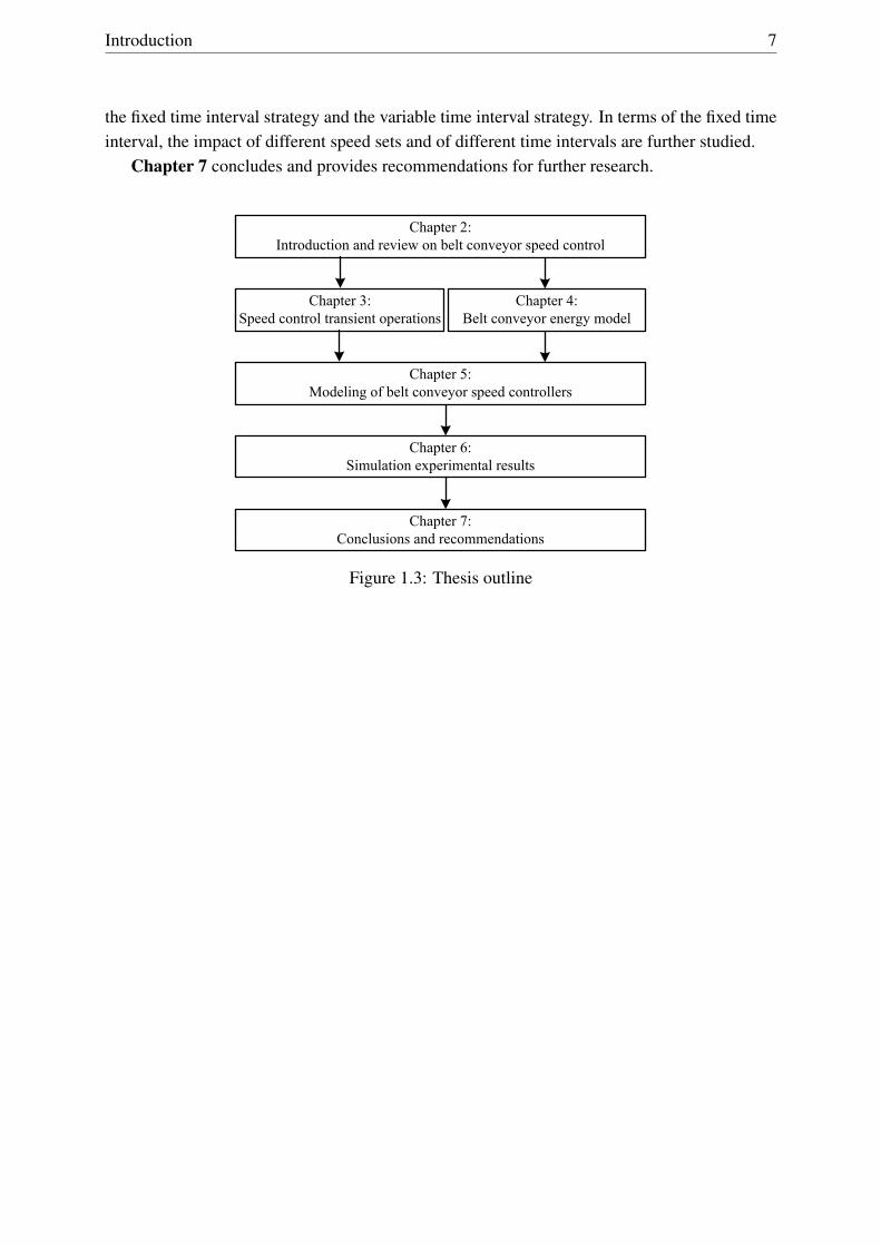
1.5 Thesis outline
The thesis outline is graphically shown in Figure 1.3.Chapter 2 introduces the speed control of belt conveyors. It includes the definition, the
principle, the classification and the prerequisites of speed control. In addition, after a literaturereview, the benefits and the challenges of speed control are analyzed in detail.
Chapter 3 presents the speed adjustment operations. Risks in transient operations are ana-lyzed, and the ECO method is introduced to determine the minimum speed adjustment time. Inaddition, the FEM-based belt model is used to analyze the conveyor’s dynamic performance intransient operations.
Chapter 4 analyzes the energy loss of belt conveyors. According to the individual energylosses along the conveyor length, a analytical model is proposed to calculate the artificial fric-tional coefficient for different loads and speeds. The variable drive system efficiency is alsotaken into account.
Chapter 5 builds the modeling of belt conveyor speed control systems. The speed adjust-ment operation discussed in Chapter 3 and the energy model introduced by Chapter 4 are takinginto account. According to different loading scenarios, the passive and active speed controllersare built, and several control strategies are taken into account. In addition, several key perfor-mance indicators are defined to assess the speed control performance.
Chapter 6 investigates the performance of speed control. Both the passive speed controland the active speed control are performed. The study of the passive speed control carries outboth the static calculations and the dynamic simulations. The active speed control accounts for
Introduction 7
the fixed time interval strategy and the variable time interval strategy. In terms of the fixed timeinterval, the impact of different speed sets and of different time intervals are further studied.
Chapter 7 concludes and provides recommendations for further research.
Chapter 2:Introduction and review on belt conveyor speed control
Chapter 3:Speed control transient operations
Chapter 4:Belt conveyor energy model
Chapter 5:Modeling of belt conveyor speed controllers
Chapter 6:Simulation experimental results
Chapter 7:Conclusions and recommendations
Figure 1.3: Thesis outline

8 Energy Saving for Belt Conveyors by Speed Control

Chapter 2
Belt conveyors and speed control
Belt conveyors have been widely used in the solid material handling and conveying systems.The extensive utilization of belt conveyor results in a large consumption of electricity. Tak-ing the economic and ecological demands into account, several power reduction solutions havebeen proposed. According to the standard DIN 22101, a certain reduction of power consump-tion can be achieved by adjusting the conveyor speed to match the material flow. The techniqueof adjusting the conveyor speed to achieve energy savings of belt conveyors is called speedcontrol. This chapter details speed control and reviews the relative researches. Section 2.1 in-troduces the basic configuration of belt conveyors in brief. Section 2.2 investigates the solutionsof power savings of belt conveyors, and classifies them into four groups: methods of applyingenergy efficient components, methods of optimizing the design, methods of recovering energy,and methods of optimizing the drive operation. Speed control belongs to the last method, andthe conception of speed control is defined in Section 2.3. The conveyor speed has a linearrelationship with the conveying capacity, and Section 2.4 discusses the principle of speed con-trol. According to different operational manners, Section 2.5 suggests that speed control canbe applied either in a passive or active way. Moreover, the active speed control can be realizedby a continuous or discrete way. No matter whether speed control is carried out passively oractively, as discussed in Section 2.6, a speed control system requires at least a speed controllerto direct the variable speed drive to match the material flow observed by a material flow sensor.After satisfying these prerequisites, speed control is expected to be applied to reduce the energyconsumption of belt conveyors. As reviewed in Section 2.7, speed control has been studied foralmost twenty years, and several important research results have been achieved. Besides thepower reduction, the implementation of speed control can achieve other additional benefits. InSection 2.8, these benefits are grouped into operational benefits, ecological benefits and eco-nomic benefits. Additionally, Section 2.8 gives an analysis of the research challenges. Someconclusions are drawn in the last section.
2.1 Basic configuration of belt conveyors
Figure 2.1 illustrates a typical belt conveyor. The moving belt carries the material towards thehead pulley. In order to overcome the motional resistances along the conveying direction, the
9

10 Energy Saving for Belt Conveyors by Speed Control
conveyor is driven by a head pulley. Generally, the drive pulley is located at the head of thebelt conveyor. Belt conveyor lengths are in the range of a few meters to tens of kilometers.In the case of long belt conveyors, intermediate drives are sometimes installed to reduce therequired belt tension. Along the conveying route, the belt is supported by a huge number ofrotating idler rollers. Between neighboring idler stations, the moving belt has a sag due to itsown weight and the material load. To reduce the sag ratio, a large pre-tension is produced by agravity take-up device. In the application shown in Figure 2.1, the take-up device is tied to thetail pulley. The gravity take-up device, or named tension weight, gives a constant belt tensionwhich is independent of the belt load. Beside the tension weight, the belt tension also can beachieved by a mechanical tensioning system, and normally the belt is pre-tensioned after thedrive pulley.
Figure 2.1: Belt conveyor components and assembly (Courtesy of ConveyorBeltGuide.com(ConveyorBeltGuide, 2016))
The research object of this thesis is the trough belt conveyor system.That is the most com-mon belt conveyor system in the industrial applications. As illustrated in Figure 2.2, the idlerstation at the carrying side consists of three equal-length rollers, and the station of return sideis composed of a two-roll “V” idler. As the figure shows, at the carrying side, two wing rollsare mounted in a defined angle λ. Together with the surcharge angle β of dry bulk material,they create a material cross section on the top of the belt. According to the standard DIN 22101(German Institute for Standardization, 2015), the nominal cross-section area Anom of a troughedbelt conveyor is determined by:
Anom =
[lm+(bc − lm)
2cosλ
](bc − lm)
2sinλ+
[lm+(bc − lm)
2cosλ
]2 tanβ4
(2.1)
where bc is the contact length of bulk material. According to DIN 22101, the contact lengthdepends on the belt width:
B ≤ 2000mm bc = 0.9B−50mm (2.2)
B > 2000mm bc = B−250mm (2.3)
Accordingly, the nominal conveying capacity Qnom is

Belt conveyors and speed control 11
Qnom = 3.6Anomρsvnom (2.4)
in which
ρs density of bulk solid material conveyed
vnom nominal speed of a belt conveyor
Carrying idler frame
Return idler frame
λ
Bulk material
Belt Center roll
Wing rollβ
b
B
lM
Figure 2.2: Troughed idler sets
2.2 Solutions for reducing energy consumption of belt con-veyors
Due to their inherent advantages, such as high capacity and low labor requirement, belt convey-ors play a significant role in bulk solids handling and conveying. According to Daniel Clénet(2010), there are more than 2.5 million conveyors operating in the world. Considering their ex-tensive use, the operations of belt conveyors involve a large amount of electricity. For instance,belt conveyors are responsible for 50% to 70% of the total electricity demand in a dry bulkterminal (Hiltermann, 2008) and about 10% of the total maximum demand in South Africa isused by bulk material handling (Marais, 2007). Furthermore, coal-fired power plants currentlyfuel 41% of the global electricity (Goto et al., 2013) and the coal makes up above 45% of theworld’s carbon dioxide emissions from fuels (International Energy Agency, 2015). Therefore,taking the economic and ecological challenges associated into account, there is a strong demandfor lowering the energy consumption of belt conveyors, and for reducing the carbon footprint.
Over the past decades, several different techniques have been proposed. Based on differentobjects of the belt conveyor, these different approaches can be classified into four groups:

12 Energy Saving for Belt Conveyors by Speed Control
• methods of applying energy efficient components, such as
– low loss conveyor belts
* low loss rubber of bottom cover (Falkenberg and Wennekamp, 2008; Gerardvan den Hondel, 2010)
* low weight belt (Lodewijks and Pang, 2013c)
– energy-saving idler stations
* low loss rollers (Mukhopadhyay et al., 2009)
* new design of idler stations, such as ESIdler (Stephens Adamson, 2014)
– energy efficient driving systems
* efficient driving units, such as frequency converters, gearboxes and motors(ABB, 2000)
• methods of optimizing the design, such as
– optimizing the route of conveyors (Yester, 1997)
– reducing the number of intermedium transfers (Alspaugh, 2004)
• methods of recovering energy, such as
– braking based re-generators (Rodriguez et al., 2002)
– driven-turbine based generators (Michael Prenner and Franz Kessler, 2012; Graaf,2013)
• and methods of optimizing the drive operation, such as
– controlling motor sequences (Dalgleish and Grobler, 2003; Levi, 2008)
– adjusting the conveyor speed (Hiltermann, 2008; Jeftenic et al., 2010; Pang andLodewijks, 2011; Ristic and Jeftenic, 2011)
In the case of installing new belt conveyors, the first two methods are effectively and efficientlyapplied to reduce the power consumption. However, in the case of well-working conveyorsthese methods require large extra investments, since they need to replace existing conveyorcomponents or change the current layout of belt conveyor systems. The third method, which at-tempts to recover the kinetic and the potential energy of the transported material, is ecologicallypromising and technically possible. However, as suggested by Graaf (2013), this method maybe not economically viable since this solution costs more money than it generates. The fourthmethod can be applied to the conveyors to be installed or the existing conveyors with limitedextra investments. Therefore, the thesis focuses on the method optimizing the drive operation,especially the method adjusting the conveyor speed.

Belt conveyors and speed control 13
As Equation 2.4 suggests, the belt conveyor’s nominal capacity is dependent on the nominalcross-section area of bulk material, the density of the bulk material and the nominal conveyorspeed. Normally, the actual material flow is generally lower than the nominal conveying ca-pacity of belt conveyors. Therefore in most cases when the belt conveyor is running at nomi-nal speed, the belt will be partly filled. As proved by Daus et al. (1998); Hiltermann (2008);Lodewijks et al. (2011), lowering belt speed can achieve considerable energy savings of beltconveyors by adjusting the conveyor speed. (Hiltermann, 2008) defined this technique as speedcontrol.
2.3 Conceptions of speed control and transient operations
Speed control is “the intentional change of the drive speed to a value within a predeterminedrate under certain conditions for specific purposes” (Anonymity, 2016). Traditionally, speedcontrol is widely applied to achieve soft start-up or stop operations. In terms of star-ups, sev-eral techniques, such as variable frequency control, variable fill hydro-kinetic coupling andvariable mechanical transmission couple, have been employed to provide acceptable start-upperformance under all belt load conditions (Nave, 1996). In addition, the sinusoidal and tri-angular acceleration profiles, individually commended by Harrison (1983) and Nordell (1987),are commonly applied to provide good dynamic performance of belt conveyors. In terms ofsoft stop operations, intelligent braking systems have been developed, which use cutting-edgetechnologies to allow a specified braking time (Al-Sharif, 2007). Moreover, the overshoot andoscillations at the end of the braking sequence can be minimized or eliminated. Differing fromthe traditional applications of speed control on belt conveyors, speed control in this thesis isapplied to adjust the conveyor speed to match the material flow, so that the power reduction ofbelt conveyors is expected to be realized. Therefore, speed control in the thesis is redefined as:a technique of adjusting the conveyor speed for the purpose of reducing energy consumption ofbelt conveyors.
The operation of adjusting speed is defined as the transient operation. In Lodewijks andPang (2013a), the operations of belt conveyors are distinguished into two types: the stationaryoperation and the transient operation. The stationary operation includes both the case where thebelt is not moving at all and the case where the belt is running at full design speed. Differingfrom the stationary operation, the transient operation normally includes the normal operationalstart, the aborted start, the normal operational stop and the emergency stop (Lodewijks andPang, 2013a). In this thesis, the definition of stationary operation is expanded into the operationwhere the belt is running at a predetermined speed and this speed can be either nominal ornon-nominal speed. In addition, the transient operations are expanded into the acceleration ordeceleration operations between neighboring stationary operations. This will be further detailedin Chapter 3.

14 Energy Saving for Belt Conveyors by Speed Control
2.4 Principle of Speed control
Belt conveyors are designed to cope with the potential peak of material flow. If it is assumedthat the conveying capacity of belt conveyor system equals the demanded maximum, then assuggested by Equation 2.4, the value of the nominal belt speed and the value of nominal cross-section area of bulk material on the belt are responsible for the maximum conveying capacity.
vnom
(a) Nominal speed
vact
(b) Non-nominal speed
Figure 2.3: Principle of speed control. vnom: nominal speed, vact : actual non-nominal speed.
Figure 2.3 illustrates the principle of speed control. Most often the belt conveyor is runningat nominal speed. In a large number of cases, the feeding rate is lower than the nominal con-veying capacity . In these cases the belt conveyor is partially filled by the dry bulk material (seeFigure 2.3a). In order to reduce the energy consumption, the conveyor speed can be reducedto follow the actual feeding rate. As shown in Figure 2.3b, the belt filling ratio is significantlyimproved due to speed control. Taking the permitted cross-section area of material on the beltinto account, the actual conveyor speed vact should satisfy the following equation
vact ≥Qact
Qnomvnom =
Aact
Anomvnom (2.5)
where
• Qact is the actual feeding rate.
• Aact is the cross-section area of material on the belt when the conveyor is running atnominal speed.
Practically the belt speeds are determined slightly higher than the required minimum belt speed,so that the risk of material overload can be prevented (Pang and Lodewijks, 2011). However,Pang and Lodewijks (2011) also suggest that the actual cross-section area of bulk solid materialon the belt conveyor is allowed to be 10% larger than the nominal for a short time period. Thesimilar suggestion is also given by Kolonja et al. (2003), since according to DIN 22101 (GermanInstitute for Standardization, 2015), the conveyor capacity is calculated on the basis of 80% ofbelt cross-section utilization.

Belt conveyors and speed control 15
2.5 Classifications of speed control
According to Hiltermann (2008), speed control of belt conveyors can be performed in two ways:passively and actively. Accordingly, speed control can be basically classified into two groups:the passive speed control and the active speed control.
In the passive speed control, the belt speed is lowered but fixed. According to the potentialpeak of material flow in the future minutes or hours, a suitable belt speed is selected prior. Tak-ing the bulk material conveying system in an import terminal for example. At the unloading areaof the land side, several ship unloaders are mounted. According to the unloader schedule, thenumber of available ship unloaders varies in time. Based on the number of operating unloadersin a certain time period, the potential peak of material flow in that time interval can be deter-mined. Then the conveyor speed can be adjusted to match the potential peak of material flowrate, or to match the number of available unloaders. The applications of the passive speed con-trol can be found in (Daus et al., 1998; Lodewijks et al., 2011; Hiltermann et al., 2011), and assuggested by Hiltermann (2008), in the applications of the passive speed control, the selectionof the belt speed is significantly responsible for the magnitude of the final energy savings.
In the active speed control, the material flow is monitored in real time. Then, accordingto the variation of the actual material rate, the conveyor speed is adjusted automatically toensure the cross-section area of bulk material on the belt to be in the greatest possible degree.According to Lodewijks et al. (2011), the active speed control can be realized in a continuousor discrete manner. However, as suggested by Pang and Lodewijks (2011), the discrete speedcontrol for belt conveyor is more preferred for practical reasons. Firstly, a continuous activespeed control needs to adjust the belt speed according to the actual material flow on the belt.When the material flow fluctuates, detrimental vibrations may occur on the belt and conveyorconstruction at certain belt speeds. The belt speed at which vibration occurs should therefore beavoided. Secondly, when the material flow fluctuates considerably, the demanded accelerationcan be larger than the permitted. An unexpected large tension can result in for instance reducingthe service life of belt. Therefore, the discrete active speed control is preferred in practice.
The passive speed control employs a fixed speed based on the expected material flow inthe future time interval. Under this control, small and/or temporary variations in the materialflow do not result in belt speed variations, so that the passive speed control is a semi-optimalmethod. The active speed control accounts for the variation of material flow. If the variation isconsiderable, the conveyor speed will be adjusted to reduce the deviation. Therefore, comparedto the passive speed control, the belt speed in active speed control is lower on average. Thereforemore energy savings are expected to be achieved by the active speed control. However, due tothe frequent speed adjustment, the active speed control has not been implemented anywhere todate in practice.

16 Energy Saving for Belt Conveyors by Speed Control
2.6 Prerequisites of speed control system
The speed control has already been proved to be effectively to reduce the energy consumptionof belt conveyors. In order to apply speed control, at least two prerequisites must be satisfied:the proper feeding conditions and the speed control systems. According to Pang et al. (2016),the feeding condition or the loading conditions can be classified into different scenarios whichwill be detailed in Section 5.1. This section mainly discusses the requirement of speed controlsystems.
Almost any modern control system contains a controller to analyze the data observed fromsensors, and to command the actuator to respond for moving or for controlling a mechanism orsystem. The speed control system is such a modern control system, of which a speed controllerdirects the variable speed drives to match the material flow observed by a material flow sensor.
2.6.1 Speed controller
Speed controller is the key of a speed control system. It analyzes the potential peak or thereal value of the material flow, and then commands the motor to keep or change the belt speed.According to different operating principles, the control system has two types: passive and activespeed control systems. In the passive speed control, the selection of conveyor speed determinesthe magnitude of energy savings of belt conveyors. Moreover, the speed curves generated bythe controller are responsible for the conveyor dynamics in transient operations. In transientoperations, especially in acceleration operation, the improper speed curves might result in forinstance the risk of belt over-tension. Therefore, the passive speed control system requires aprecise selection of belt speed and a good speed curve generator. Comparing with the passivespeed control, the active speed control is more complex, since in the active speed control, thebelt speed might be more frequently adjusted to match the variable material flow. Moreover,differing with the passive speed controller which generally is an open-loop controller, the activespeed controller can be either an open-loop or closed-loop controller.
2.6.2 Variable speed drives
Variable speed drives are the actuator of the speed control system, and they are having beenwidely used for achieving soft start-ups of belt conveyors. Variable speeds can be realized byemploying mechanical or electronic devices (see Figure 2.4). According to Conveyor Equip-ment Manufacturers Association (2005), the common mechanical methods of obtaining variablespeeds are: V-belt drives on variable pitch diameter sheaves or pulleys, variable-speed trans-mission, and variable-speed hydraulic couplings. The electrical variable speed drivers mainlyrely on the variable frequency converter, which varies the motor input frequency and voltageto control the alternating-current (AC) motor’s speed and torque. Comparing with other vari-able speed drivers, the variable frequency converter based drivers behave more efficiently, andcan drive belt conveyors in specialized patterns to further minimize mechanical and electricalstress. Especially in the active speed control where the conveyor speed is frequently adjusted,

Belt conveyors and speed control 17
the frequency-controller drive shows a good controllability in speed adjustment operations.
(a) (b) (c)
(d)
Figure 2.4: Variable speed drivers. (a) V-belt drives, courtesy of Barnes (2003). (b) Variable-speed transmission, courtesy of Ricardo (2010). (c) Variable-speed hydraulic coupling, courtesyof Encyclopedia (2010). (d) Variable frequency drives, courtesy of Fluke Corporation (2016).
(a) (b)
Figure 2.5: Material flow sensors. (a) Belt scale, courtesy of FLSmidth Pfister Limited (2017).(b) Laser profilometer, courtesy of SICK B.V. (2017).
2.6.3 Material mass/volume sensor device
The material flow can be detected by a sensor. In the passive speed control, the value of materialflow rate is detected to ensure that the material loading rate is no larger than the permittedconveying rate, so that the belt’s overburden can be avoided. In the active speed control, the

18 Energy Saving for Belt Conveyors by Speed Control
material feeding rate is monitored in real time, so that the belt speed can be precisely adjustedto match the variable flow rate. In addition, the actual value of material flow can be used toestimate the power consumption of belt conveyors, and to evaluate the power savings by meansof speed control. The material flow rate can be measured either by belt weighers or volumeflow sensors. According to different principles, the material flow rate can be measured by a beltscale (Figure 2.5a) or by a laser profilometer (Figure 2.5b).
2.6.4 Others
Besides above discussed components, some other accessories also contributes to improve theperformance of speed control. For example, extra cooling fans are recommended to improve thecooling effect of shaft-mounted radial fan on the AC motor, especially when operating speedsare reduced more than 50%. In addition, variable geometry discharge chutes are required toavoid severe wear of the chute, since varying the belt speed changes the material dischargeparabola at the discharge points.
2.7 Review on academic research and industrial applications
Previous sections briefly described the belt conveyor speed control. This section will review itsacademic researches, including the industrial applications. Researches on belt conveyor speedcontrol can be distinguished into three aspects. The first aspect is characterized by the viabilityanalysis of speed control for the purpose of energy savings. Subsequently, the developmentis continued by exploiting different control algorithms of speed control and investigating theefficacy of different forms of speed control.
2.7.1 Aspect I- Analyzing the viability of speed control
The research of viability analysis of speed control can be dated back to a report by Daus et al.(1998), in which a new conveying and loading system was installed to replace the old one. Aload-dependent belt-speed adjustment system was developed in order to achieve energy sav-ings of the new conveyor system. According to the standard DIN 22101 (German Institute forStandardization, 2015), the kinetic resistance F could be approximated by
F = C f L(m′roll +
(2m′belt +m′bulk
)cosδ
)g+Hm′bulkg (2.6)
in which
C the coefficient of secondary resistances
f the artificial coefficient of frictional resistances
L the conveying length of conveyor
m′roll the mass of idler rolls in unit length

Belt conveyors and speed control 19
m′belt the linear density of belt
m′bulk the linear density of bulk material
δ the inclination angle of a belt conveyor
g gravity acceleration
H the height difference between the loading and unloading areas of a belt conveyor
Then taking the conveyor speed v and the efficiency ηsys of the driving system into account, therequired electrical power was
Pe =Fvηsys=
1ηsys
[C f L
(m′roll +2m′belt
)gv+ (C f Lg+Hg)
(m′bulkv
) ]=
1ηsys
[C f L
(m′roll +2m′beltcosδ
)gv+ (C f Lgcosδ+Hg)Qact
3.6
](2.7)
If it was assumed that the values of f and ηsys were constant at different temperatures andspeeds, then Equation 2.7 yielded that the energy consumption was lowered over a reduction ofbelt speed. Accordingly, the theoretical viability of speed control was determined. Moreover,from Equation 2.7 it can be learned that, the principle behind power savings by means of speedcontrol is to reduce the movement of idler rolls and the belt.
The viability of belt conveyor speed control was also determined by physical experiments.Hiltermann (2008) performed measurements at a dry bulk terminal. Both the material loadingrate and the conveyor speed were manually altered. Power consumption was measured by usinga digital clam meter to detect the input power of a frequency converter. Figure 2.6 illustrates theexperimental result. The data clearly shows that the operation running at a higher belt speedshad consumed more power as compared to that running at a lower speed. Accordingly, speedcontrol had successfully allowed the power reduction of the concerned belt conveyor.
2.7.2 Aspect II- Developing speed control algorithms
In order to improve the energy efficiency of belt conveyors, several speed control algorithmshave been developed. Daus et al. (1998) introduced an algorithm in which the conveyor speedwas determined by the number of excavators in use. This algorithm is simple and can be detailedby the following equation:
actual belt speed=
50% nominal belt speed 1 excavator
75% nominal belt speed 2 excavators
100% nominal belt speed 3-4 excavators
(2.8)
This algorithm can be applied in the passive speed control, in which the deviation of materialflow rate in a certain time period can be ignored.

20 Energy Saving for Belt Conveyors by Speed Control
0
50
100
150
200
250
300
350
400
450
500
550
600
0 500 1000 1500 2000 2500 3000 3500 4000 4500 5000 5500 6000
Ele
ctr
ical d
rive
po
we
r (k
W)
Material flow (MTPH)
US Steam Coal (805kg/m3) - 4,5 m/s
US Steam Coal (805kg/m3) - 3,6 m/s
US Steam Coal (805kg/m3) - 2,4 m/s
Australian Steam Coal (867kg/m3) - 4,8 m/s
Australian Steam Coal (867kg/m3) - 4,5 m/s
Australian Steam Coal (867kg/m3) - 4,05 m/s
Australian Steam Coal (867kg/m3) - 3,6 m/s
Australian Steam Coal (867kg/m3) - 3 m/s
Sepetiba Iron Ore (2442kg/m3) - 4,5 m/s
Sepetiba Iron Ore (2442kg/m3) - 4,05 m/s
Sepetiba Iron Ore (2442kg/m3) - 3,6 m/s
Sepetiba Iron Ore (2442kg/m3) - 3 m/s
Figure 2.6: Measured electrical power of the studied belt conveyor. Courtesy of Hiltermann(2008).
As suggested by Hiltermann (2008), the passive speed control normally results in less en-ergy savings than active speed control, especially in cases where the material flow has a con-siderable deviation. However, the active speed control might result in continuous high belttension. Therefore, rather that in a continuous speed manner, the active speed control in prac-tice prefers to work in a discrete manner. Pang and Lodewijks (2011) proposed fuzzy control,as one control method based on fuzzy logic to provide discrete control strategy, to discretizethe operations of speed control. Pang and Lodewijks (2011) defined a finite number of fuzzyboundaries bn(n = 1,2, ...,n) in the percentage of nominal conveying capacity. If a value x wasin the range [bi,bi+1), the fuzzy membership function was constructed as
fbi+1 (x) =bi+1− xbi+1− bi
(2.9)
fbi (x) =x− bi
bi+1− bi(2.10)
wherefbi (x)+ fbi+1 (x) = 1 (2.11)
As shown in Figure 2.7a, the fuzzy values, derived from Equations 2.9 and 2.10, shows theposition of a determined material loading rate within its range. Pang and Lodewijks (2011)further suggested that the adjustment of belt speed was determined based on the comparisonof the fuzzy values of fbi (x) and fbi+1 (x). Taking the case shown in Figure 2.7b for example,the conveyor was running at speed vi+1 in the case of the scenario fbi+1 (x) > fbi (x). When the
Belt conveyors and speed control 21
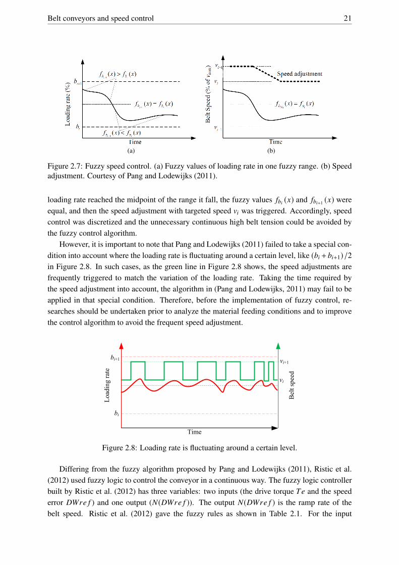
(a) (b)
Figure 2.7: Fuzzy speed control. (a) Fuzzy values of loading rate in one fuzzy range. (b) Speedadjustment. Courtesy of Pang and Lodewijks (2011).
loading rate reached the midpoint of the range it fall, the fuzzy values fbi (x) and fbi+1 (x) wereequal, and then the speed adjustment with targeted speed vi was triggered. Accordingly, speedcontrol was discretized and the unnecessary continuous high belt tension could be avoided bythe fuzzy control algorithm.
However, it is important to note that Pang and Lodewijks (2011) failed to take a special con-dition into account where the loading rate is fluctuating around a certain level, like (bi + bi+1)/2in Figure 2.8. In such cases, as the green line in Figure 2.8 shows, the speed adjustments arefrequently triggered to match the variation of the loading rate. Taking the time required bythe speed adjustment into account, the algorithm in (Pang and Lodewijks, 2011) may fail to beapplied in that special condition. Therefore, before the implementation of fuzzy control, re-searches should be undertaken prior to analyze the material feeding conditions and to improvethe control algorithm to avoid the frequent speed adjustment.
bi
bi+1
Load
ing
rate
Bel
t spe
ed
Time
vi+1
vi
Figure 2.8: Loading rate is fluctuating around a certain level.
Differing from the fuzzy algorithm proposed by Pang and Lodewijks (2011), Ristic et al.(2012) used fuzzy logic to control the conveyor in a continuous way. The fuzzy logic controllerbuilt by Ristic et al. (2012) has three variables: two inputs (the drive torque Te and the speederror DWre f ) and one output (N(DWre f )). The output N(DWre f ) is the ramp rate of thebelt speed. Ristic et al. (2012) gave the fuzzy rules as shown in Table 2.1. For the input
22 Energy Saving for Belt Conveyors by Speed Control
variable Te, if the driving torque is close to zero, narrow fuzzy sets are required to improve thecontrol sensitivity and to avoid the braking operation donated by the fuzzy element “N”. For anypositive value of the Te, if the input variable DWre f is positive, then the fuzzy controller gavethe output a big value N(DWre f ) so that the conveyor could have a dramatic increase to avoidmaterial spillage away from the belt. For the value of DWre f , if the speed deviation is limited,the system had no sudden change of N(DWre f ) so that the continuous high belt tension couldbe avoided.
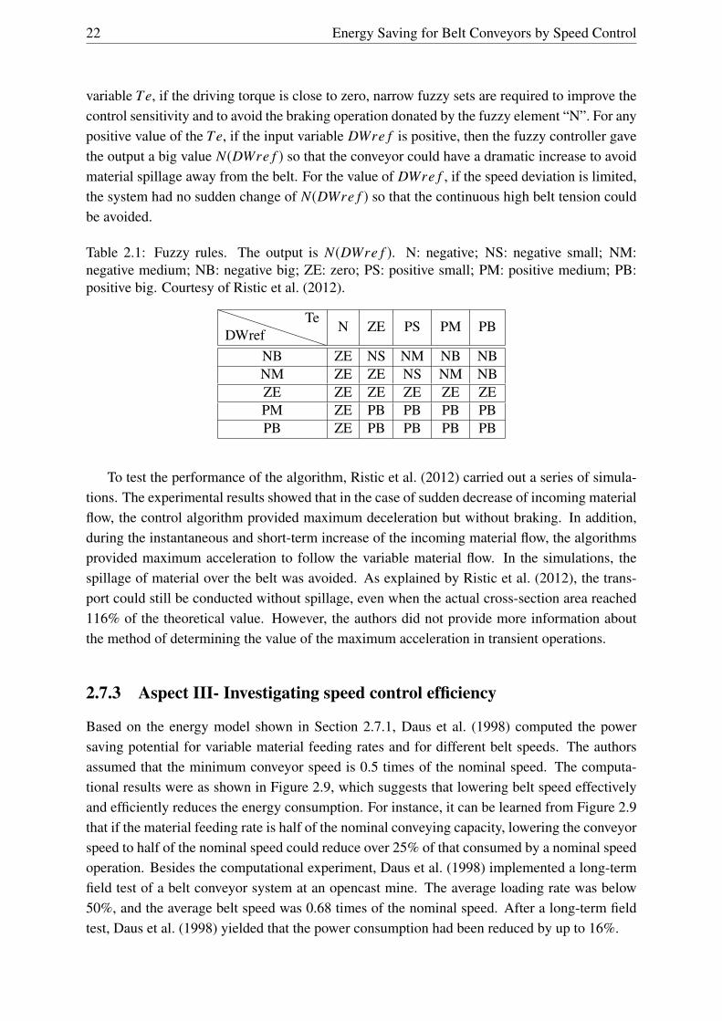
Table 2.1: Fuzzy rules. The output is N(DWre f ). N: negative; NS: negative small; NM:negative medium; NB: negative big; ZE: zero; PS: positive small; PM: positive medium; PB:positive big. Courtesy of Ristic et al. (2012).
DWrefTe
N ZE PS PM PB
NB ZE NS NM NB NBNM ZE ZE NS NM NBZE ZE ZE ZE ZE ZEPM ZE PB PB PB PBPB ZE PB PB PB PB
To test the performance of the algorithm, Ristic et al. (2012) carried out a series of simula-tions. The experimental results showed that in the case of sudden decrease of incoming materialflow, the control algorithm provided maximum deceleration but without braking. In addition,during the instantaneous and short-term increase of the incoming material flow, the algorithmsprovided maximum acceleration to follow the variable material flow. In the simulations, thespillage of material over the belt was avoided. As explained by Ristic et al. (2012), the trans-port could still be conducted without spillage, even when the actual cross-section area reached116% of the theoretical value. However, the authors did not provide more information aboutthe method of determining the value of the maximum acceleration in transient operations.
2.7.3 Aspect III- Investigating speed control efficiency
Based on the energy model shown in Section 2.7.1, Daus et al. (1998) computed the powersaving potential for variable material feeding rates and for different belt speeds. The authorsassumed that the minimum conveyor speed is 0.5 times of the nominal speed. The computa-tional results were as shown in Figure 2.9, which suggests that lowering belt speed effectivelyand efficiently reduces the energy consumption. For instance, it can be learned from Figure 2.9that if the material feeding rate is half of the nominal conveying capacity, lowering the conveyorspeed to half of the nominal speed could reduce over 25% of that consumed by a nominal speedoperation. Besides the computational experiment, Daus et al. (1998) implemented a long-termfield test of a belt conveyor system at an opencast mine. The average loading rate was below50%, and the average belt speed was 0.68 times of the nominal speed. After a long-term fieldtest, Daus et al. (1998) yielded that the power consumption had been reduced by up to 16%.
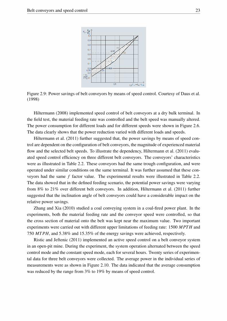
Belt conveyors and speed control 23
Figure 2.9: Power savings of belt conveyors by means of speed control. Courtesy of Daus et al.(1998)
Hiltermann (2008) implemented speed control of belt conveyors at a dry bulk terminal. Inthe field test, the material feeding rate was controlled and the belt speed was manually altered.The power consumption for different loads and for different speeds were shown in Figure 2.6.The data clearly shows that the power reduction varied with different loads and speeds.
Hiltermann et al. (2011) further suggested that, the power savings by means of speed con-trol are dependent on the configuration of belt conveyors, the magnitude of experienced materialflow and the selected belt speeds. To illustrate the dependency, Hiltermann et al. (2011) evalu-ated speed control efficiency on three different belt conveyors. The conveyors’ characteristicswere as illustrated in Table 2.2. These conveyors had the same trough configuration, and wereoperated under similar conditions on the same terminal. It was further assumed that these con-veyors had the same f factor value. The experimental results were illustrated in Table 2.2.The data showed that in the defined feeding scenario, the potential power savings were varyingfrom 8% to 21% over different belt conveyors. In addition, Hiltermann et al. (2011) furthersuggested that the inclination angle of belt conveyors could have a considerable impact on therelative power savings.
Zhang and Xia (2010) studied a coal conveying system in a coal-fired power plant. In theexperiments, both the material feeding rate and the conveyor speed were controlled, so thatthe cross section of material onto the belt was kept near the maximum value. Two importantexperiments were carried out with different upper limitations of feeding rate: 1500 MPTH and750 MTPH, and 5.38% and 15.35% of the energy savings were achieved, respectively.
Ristic and Jeftenic (2011) implemented an active speed control on a belt conveyor systemin an open-pit mine. During the experiment, the system operation alternated between the speedcontrol mode and the constant speed mode, each for several hours. Twenty series of experimen-tal data for three belt conveyors were collected. The average power in the individual series ofmeasurements were as shown in Figure 2.10. The data indicated that the average consumptionwas reduced by the range from 3% to 19% by means of speed control.

24 Energy Saving for Belt Conveyors by Speed Control
Table 2.2: Belt conveyor characteristics and speed control savings. Courtesy of Hiltermannet al. (2011).
Parameters Case 1 Case 2 Case 3Length (m) 660 1,410 95
Material lifting height (m) 46.1 5.8 9.0width (mm) 1,800 1,800 1,800
Trough angle (°) 40 40 40Nominal speed (m/s) 4.5 4.5 4.5
Nominal capacity (MPTH) 6,000 6,000 6,000Pe(6,000 MPTH) (kW) 722 657 261
Pe(3,250 MPTH, 4.5 m/s) (kW) 449 471 156Pe(3,250 MPTH, 2,75 m/s) (kW) 400 373 144
Pe,savings(kW) 49 98 12Pe,savings(%) 11 21 8
Figure 2.10: Average power consumption of belt drives on the third, fourth, and fifth belt con-veyor stations (B3, B4, and B5): white bars—constant speed operation, gray bars—variablespeed operation with fuzzy logic control. Courtesy of Ristic and Jeftenic (2011).

Belt conveyors and speed control 25
2.8 Benefits and challenges of speed control
According to the experimental results shown in Section 2.7, a certain amount of power reductionof belt conveyors can be achieved by speed control. Besides energy savings, the implementationof speed control can achieve other additional benefits, including operational benefits, ecologicalbenefits and economic benefits. In terms of the operational benefits, speed control results ina considerable reduction in the wear rate of the system (Hiltermann, 2008; A.P. Wiid et al.,2009; Lodewijks et al., 2011). Taking the belt for instance, since material has to be acceleratedless in the loading and accelerating areas, less wear will behave on the top rubber of belt. Inaddition, the variable speed operation presents a benefit in the expected pulley performance onbasis of dynamic life expectancy. Therefore, speed control results in operational benefits of beltconveyors.
In terms of ecological benefits, due to lower average belt speed and reduced surface area pertransported unit of material, less dust will be produced. Then dust emissions can be significantlyreduced (Hiltermann, 2008). Moreover, the emissions of pollutants and greenhouse gases fromfossil-based electricity generations can be lowered as a consequence, due to less electrical powerconsumption.
In terms of economic benefits, less power consumption of belt conveyors leads a reductionof electricity cost. In addition, if we take the social cost into account, a great reduction of socialcosts of environmental pollution can be achieved by speed control. Moreover, due to the longerservice life time of conveyor components, such as pulleys, a reduction of maintenance costs canbe achieved by speed control. This is also suggested by Daus et al. (1998) and (Hiltermann,2008).
However, according to the literature survey, implementations of speed control that can befound in practice to reduce energy consumption are rare. Some problems of previous researcheson speed control have not been handled. These major problems can be classified into two as-pects. From the control aspect, previous research does not cover some issues, like the potentialrisks and the dynamic analysis of belt conveyors in transient operations. In previous researches,both Pang and Lodewijks (2011) and Ristic and Jeftenic (2011) suggested that the maximum ac-celeration should be limited to avoid unhealthy conveyor dynamics. However, these researchesdid not provide any general method of determining the permitted maximum acceleration of beltconveyors. From the energy saving aspect, the current power calculations use the constant ffactor value, derived from DIN 22101, to estimate the power savings by means of speed control.However, more researches show that the f factor value varies with loads and speeds. Therefore,it is highly suggested to use the variable f factor values to improve the evaluation, instead ofthe constant f factor value.
This thesis aims to investigate the application of speed control on a belt conveyor, especiallyon improving the performance of a belt conveyor in terms of dynamics and economics. Basedon the above mentioned research problems, this research is striving to overcome the followingchallenges:
(i) Providing a method to determine the permitted maximum acceleration and the requestedminimum acceleration time.

26 Energy Saving for Belt Conveyors by Speed Control
(ii) Seeking an a method of calculating the DIN f factor values for different loads and forspeeds.
2.9 Conclusion
This chapter described the belt conveyor speed control, and reviewed the academic researchesand the industrial applications. From the literature, it can be concluded that speed control is apromising approach of reducing power consumption of belt conveyors. The literature researchfurther suggests that previous researches did not cover some issues like potential risks and thedynamic performance of belt conveyors in transient operations. Moreover, the literature reviewindicates that the current research on speed control faces two major challenges: providing amethod to determine the requested minimum speed adjustment time to ensure healthy dynamicsof a belt conveyor during transient operations, and seeking an accurate energy model to assessthe belt conveyor speed control. Taking these challenges into account, Chapter 3 will study thetransient operations, and the belt conveyor energy model will be studied in Chapter 4.

Chapter 3
Speed control transient operations
Chapter 2 presented an overview of the academic researches of belt conveyor speed control. Asthe previous chapter concluded, the speed control of a belt conveyor lacks applicability, sincethe previous researches rarely took the conveyor dynamics in transient operations into account.This chapter is going to investigate the transient operations of belt conveyors. To improve theconveyor dynamic performance, a new method will be proposed to determine the minimumspeed adjustment time in transient operations.
This chapter is based on (He et al., 2016a,b,c).
3.1 Introduction
When considering the operational conditions, Lodewijks and Pang (2013a) defined the oper-ations of belt conveyors, and distinguished these operations into two groups: the stationaryoperation and the transient operation. The stationary operations include two cases: the casewhere the belt is totally stopped, and the case where the belt is running at a steady state speed.Conventially, belt conveyors are running at nominal speed. Due to speed control, the belt con-veyor however is often running at non-nominal speed to match the actual material feeding rate.Therefore, as shown in Figure 3.1, the applications of stationary operations in this thesis areextended into three cases. If we do not take into account other issues, such as the efficiencyof the driving system, the non-nominal speed can be any value between zero and the nominalspeed.
Besides the stationary operation, Lodewijks and Pang (2013a) further defined the transientoperation which normally includes the following situations:
• Normal operational start. A normal operational start is a start where the belt conveyoris started as planned. In a conventional normal operational start, a motor can be startedsimply by a direct online starter which directly connects the motor terminals to the powersupply. This however only works for belt conveyors with motor power up till about 15kW . Nowadays, variable speed drives are widely applied to control the conveyor speed inthe starting procedure to realize a soft start-up.
• Aborted start. An aborted start is an abnormal operational start in which the start-up is
27

28 Energy Saving for Belt Conveyors by Speed Control
vnom
Bel
t spe
ed
0time
The case where the belt is running at nominal speed.
The case where the belt is running at non-nominal speed.
The case where the belt is fully stopped.
Figure 3.1: Cases of stationary operations.
accidentally terminated before the conveyor reaches the full designed speed. This can becaused by the thermal overload of the drives, serious deviation between the planned andthe actual belt speed profiles, serious misalignment of the belt triggering a misalignmentswitch, a power outage or an operator manually switching the power supply off.
• Normal operational stop. A normal operational stop is a stop where the belt is stoppedin a planned manner. Similar to the normal operational start, the normal operation stopcan be realized either in a non-controlled or controlled manner. In a non-controlled stop,the power supply of motor is switched off and then the conveyor belt drifts to rest. In acontrolled normal stop, the drive torque or the velocity is controlled. In the cases wherethe drive torque is controlled the drive forces are kept constant but less than the motionalresistances. In another case where the velocity is controlled, the velocity is monitoredin real time and the variable drive torque ensures the velocity decreasing as the designedrules (such as a sinusoidal deceleration profile). In such cases, the stop time can beindependent of the bulk material mass loaded on the belt, as long as it is longer than thebelt drift time.
• Emergency stop. When an emergency event occurs, for example the belt is slippingaround the drive pulley, an emergency stop is carried out so that the belt can be stoppedin a short period of time. During an emergency stop a brake may be applied.
Similarly, the applications of transient operations can be further expanded in this thesis. In thecase of belt conveyors under speed control for the purpose of power reduction, the belt conveyoris often running at a defined speed. If the material feeding rate has a considerable change, thebelt conveyor should speed up or slow down to match the actual material flow rate. Here, theoperation between adjacent stationary operations is defined as the transient operation. As shownin Figure 3.2, the transient operations include both the accelerating and decelerating processes.
A healthy transient operation is an important prerequisite of belt conveyor speed control.The performance of transient operations has a significant impact on the service life of conveyorcomponents. High ramp rate of adjusting the belt speed causes very high tensions in the belt,
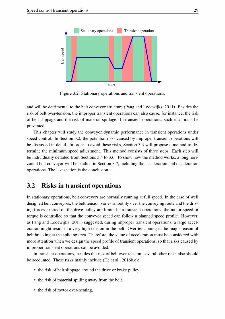
Speed control transient operations 29
time
Bel
t spe
ed
Stationary operations Transient operations
Figure 3.2: Stationary operations and transient operations.
and will be detrimental to the belt conveyor structure (Pang and Lodewijks, 2011). Besides therisk of belt over-tension, the improper transient operations can also cause, for instance, the riskof belt slippage and the risk of material spillage. In transient operations, such risks must beprevented.
This chapter will study the conveyor dynamic performance in transient operations underspeed control. In Section 3.2, the potential risks caused by improper transient operations willbe discussed in detail. In order to avoid these risks, Section 3.3 will propose a method to de-termine the minimum speed adjustment. This method consists of three steps. Each step willbe individually detailed from Sections 3.4 to 3.6. To show how the method works, a long hori-zontal belt conveyor will be studied in Section 3.7, including the acceleration and decelerationoperations. The last section is the conclusion.
3.2 Risks in transient operations
In stationary operations, belt conveyors are normally running at full speed. In the case of welldesigned belt conveyors, the belt tension varies smoothly over the conveying route and the driv-ing forces exerted on the drive pulley are limited. In transient operations, the motor speed ortorque is controlled so that the conveyor speed can follow a planned speed profile. However,as Pang and Lodewijks (2011) suggested, during improper transient operations, a large accel-eration might result in a very high tension in the belt. Over-tensioning is the major reason ofbelt breaking at the splicing area. Therefore, the value of acceleration must be considered withmore attention when we design the speed profile of transient operations, so that risks caused byimproper transient operations can be avoided.
In transient operations, besides the risk of belt over-tension, several other risks also shouldbe accounted. These risks mainly include (He et al., 2016b,c):
• the risk of belt slippage around the drive or brake pulley,
• the risk of material spilling away from the belt,
• the risk of motor over-heating,

30 Energy Saving for Belt Conveyors by Speed Control
• and the risk of pushing the motor into the regenerative operation.
3.2.1 Belt breaking at the splicing area
Figure 3.3: Belt breaking at the splicing area. Courtesy of BMG (2016).
The belt strength is mainly determined by the strength of its carcass. For a certain conveyorbelt, the belt tension rating is a given and thus constant. However, as Nordell (1998) stated,“the chain is only as strong as its weakest link. In conveyor belts,... the weak link is thesplice”. Figure 3.3 illustrates an example of belt breaking at the splicing area. As the standardDIN 22101 (German Institute for Standardization, 2015) suggests, the maximum safe workingtension is far less than the belt rating due to issues such as splice fatigue and degradation. InDIN 22101, the ratio between the working tension and the actual breaking tension is referredto as the service factor or safety factor (SF). Accordingly, the ratio between the maximum safeworking tension and the breaking tension is referred to as the minimum safety factor:
SA,min =Tmax,A
kN(3.1)
SB,min =Tmax,B
kN(3.2)
where
SA,min minimum safety factor in the steady operating condition
SB,min minimum safety factor in transient operations
Tmax,A maximum safe working tension in the steady operating condition in kN
Tmax,B maximum safe working tension in transient operations in kN
kN belt tension rating, minimum breaking strength in kN
DIN 22101 suggests that the requested minimum safety factor is determined by three importantfactors:

Speed control transient operations 31
• the dynamic fatigue strength behaviors of the belt splice
• the influence of additional belt elongations resulted from the belt deflections on pulleys,the commencement and termination of troughing, change of the direction and transitioncurves
• and the peak belt loading which only occurs temporarily, such as during start-up or stopoperations
As DIN 22101 further suggests, the value of minimum safety factors can be calculated by
SA,min =1
1−(r0+ r1)(3.3)
SB,min =1
1−(r0+ r1+ r2)(3.4)
where
r0 a basic reduction which takes the dynamic fatigue strength of the belt splice intoaccount
r1 the reduction factor taking the belt elongation into account
r2 a reduction taking the peak belt loading in transient operations into account
Table 3.1 illustrates the minimum values of safety factors and of reductions related to the beltjoint. According to the data in Table 3.1, the belt conveyor should be designed with belt ratinglarger than 8.0 times of maximum belt tension in stationary operations under normal operatingconditions. Moreover, in transient operations under normal operating conditions, the maximumbelt tension should be no larger than 1/5.4 times of the belt rating. Otherwise, it increases therisk of belt over-tension.
Table 3.1: Minimum value of the safety factor S and of the reductions r related to the belt joint.Courtesy of DIN 22101 (German Institute for Standardization, 2015).
Belt type Operating conditions r0 r1 r2 SA,min SB,min
FabricsFavorable ≥0.691 ≥0.100 ≥0.060 4.8 6.7Normal ≥0.715 ≥0.100 ≥0.060 5.4 8.0
Unfavarble ≥0.734 ≥0.100 ≥0.060 6.0 9.5
Steel cordFavorable ≥0.641 ≥0.150 ≥0.060 4.8 6.7Normal ≥0.665 ≥0.150 ≥0.060 5.4 8.0
Unfavarble ≥0.684 ≥0.150 ≥0.060 6.0 9.5
In transient operations, an excessive speed ramp rate is an important reason of belt over-tensioning. Taking the case in Figure 3.4 for instance. In the stationary operations, the belttension T1 before the drive pulley equals the belt tension T2 after the drive pulley plus the drivingforces Fd: T1 = T2+Fd . However, extra driving forces are required to overcome the inertia Fac

32 Energy Saving for Belt Conveyors by Speed Control
in acceleration operations, and the belt tension T1 arises subsequently: T1,a = T2 + Fd + Fac. Ifthe value of acceleration is large, then the value of T1 may exceed the maximum safe workingtension. That leads to belt over-tension which may cause breakage of the belt splice. In addition,the belt over-tension can also reduce the life of pulleys. Therefore, the belt tension must belimited to a safe level in transient operations.
T1
T2
Fd
Figure 3.4: Forces around the drive pulley.
3.2.2 Belt slippage around the drive pulley
The rationale of power transmission between the drive pulley and the conveyor belt is the fric-tional connection between the drive pulley and the belt. However, as suggested by Euler (1762)and Entelwein (1832), the friction between the drive pulley and the belt is limited, and that beltslippage occurs whenever the driving force attempts to exceed the available friction. Attaway(1999) and Nel and Shortt (1999) detail the calculation of the maximum available frictionalforces.
T1
T2
α
ω
0
(a)
TT+dTμdFN
dFN
x
y
dθ
(b)
Figure 3.5: Principle of the friction drive of the belt conveyor. Courtesy of Attaway (1999).
The basic of the calculation is the integration of the frictional forces around the drive pulley.Taking the case in Figure 3.5 for instance where the pulley drives the belt clockwise. Figure 3.5billustrates a belt in a finite length bending over a small segment of the driving pulley in an angledθ. As the diagram shows, the tension in the belt increases from T to T + dT . Assuming that

Speed control transient operations 33
the normal force is dFN . If it is further assumed that frictional coefficient between the belt andthe drive pulley is µ, then the maximum frictional force is µdFN without belt slippage. Takingthe forces distributed on the belt into account, the forces in the x direction can be equated by∑
Fx = 0 (3.5)
Tcosdθ2+ µ (dFN )− (T + dT)cos
dθ2= 0 (3.6)
Since the angle of dθ is very small and cos dθ2 ≈ 1, Equation 3.6 can be reduced to
µdFN = dT (3.7)
Similarly, the forces in the y direction can be equated by∑Fy = 0 (3.8)
dFN −(T + dT) sindθ2−Tsin
dθ2= 0 (3.9)
which reduces todFN = Tdθ (3.10)
since sin dθ2 ≈ 0. Then substituting Equation 3.10 into 3.7 yields
dTT= µdθ (3.11)
Then the integration over the total contact angle α gives :
T1,maxˆ
T2
dTT=
αˆ
0
udθ (3.12)
which yields the maximum belt tension without slippage:
T1,max = T2eµα (3.13)
Accordingly, the maximum value of the available frictional forces is
Ff ,max = Fd,max = T1,max −T2 = T2 (eµα −1) (3.14)
and the belt is slipping around the drive pulley whenever the driving forces exceed the maximumavailable frictional forces between the belt and the drive pulley.
If belt slippage occurs then the drive fails to drive the belt as planned, since the availabledriving force is less than the required. If the belt slippage continues to the extent that it slowsdown the conveyor, then blockage of the belt’s feeder chute or material spillage may occur.Moreover, the relative movement wears out the bottom cover of the belt and the surface cover

34 Energy Saving for Belt Conveyors by Speed Control
Figure 3.6: Pieces of a head pulley’s rubber lagging were frequently torn loose due to the beltslippage around the drive pulley. Courtesy of Belzona (2016).
of the drive pulley. A slipping pulley wears more rapidly by the heat generated as it slips (seeFigure 3.6). Besides the wear of covers, the accumulative heat may cause the damage to thecarcass and the splice. Moreover, there is an increased danger of fire if the slippage continuesfor a long period of time, especially in an environment with coal dust. Nel and Shortt (1999)mentioned a case where the belt slippage set the conveyor on fire and the fire totally destroyedthe conveyor. Unscheduled stops lead to a negative financial impact caused by lots of revenue.Therefore, the driving forces in transient operations must be restricted to avoid the risk of beltslippage and to keep the operation uninterrupted.
3.2.3 Material spillage away from the belt
Even though a belt conveyor is carefully designed, spillage from the carrying side of the beltmay occur at the loading point and elsewhere along the belt conveyor. There are many reasonsthat cause the spillage, such as the material off-center loading at the transfer points and the beltmistracking along the conveying route. Here, the focus is on the unnecessary spillage causedby improper transient operations.
In the case of belt conveyors with large speed fluctuations, the instantaneous conveyingcapacity can be less than the actual loading rate, so that the belt at the loading area may beoverloaded. This can lead to the escape of bulk materials from the belt. Both the excessivelylow and the excessively high belt tension can result in the material spillage. In transient oper-ations, the belt tension is varying along the conveying route and fluctuating over time. On onehand, if the improper transient operation results in excessively low belt tension, the belt maydrop significantly between neighboring idler stations. According to Conveyor Equipment Man-ufacturers Association (2005), material may spill over the edges of the belt when the conveyorbelt sags more than 3 percent of the span between idlers, see Figure 3.7a. On the other hand, inthe case of dipping belt conveyors, the large belt tension can lead to the lift of the belt from theidler stations, see Figure 3.7b. The lift also can cause the material spillage away from the belt.
If the material escapes from the carrying belt, it may land on the return side of the belt.
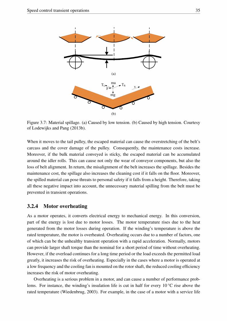
Speed control transient operations 35
(a)
mg
TRTLma
vF
(b)
Figure 3.7: Material spillage. (a) Caused by low tension. (b) Caused by high tension. Courtesyof Lodewijks and Pang (2013b).
When it moves to the tail pulley, the escaped material can cause the overstretching of the belt’scarcass and the cover damage of the pulley. Consequently, the maintenance costs increase.Moreover, if the bulk material conveyed is sticky, the escaped material can be accumulatedaround the idler rolls. This can cause not only the wear of conveyor components, but also theloss of belt alignment. In return, the misalignment of the belt increases the spillage. Besides themaintenance cost, the spillage also increases the cleaning cost if it falls on the floor. Moreover,the spilled material can pose threats to personal safety if it falls from a height. Therefore, takingall these negative impact into account, the unnecessary material spilling from the belt must beprevented in transient operations.
3.2.4 Motor overheating
As a motor operates, it converts electrical energy to mechanical energy. In this conversion,part of the energy is lost due to motor losses. The motor temperature rises due to the heatgenerated from the motor losses during operation. If the winding’s temperature is above therated temperature, the motor is overheated. Overheating occurs due to a number of factors, oneof which can be the unhealthy transient operation with a rapid acceleration. Normally, motorscan provide larger shaft torque than the nominal for a short period of time without overheating.However, if the overload continues for a long time period or the load exceeds the permitted loadgreatly, it increases the risk of overheating. Especially in the cases where a motor is operated ata low frequency and the cooling fan is mounted on the rotor shaft, the reduced cooling efficiencyincreases the risk of motor overheating.
Overheating is a serious problem in a motor, and can cause a number of performance prob-lems. For instance, the winding’s insulation life is cut in half for every 10 °C rise above therated temperature (Wiedenbrug, 2003). For example, in the case of a motor with a service life
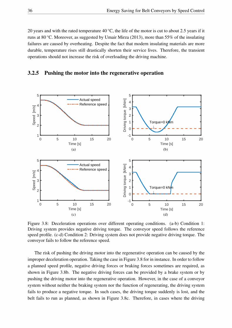
36 Energy Saving for Belt Conveyors by Speed Control
20 years and with the rated temperature 40 °C, the life of the motor is cut to about 2.5 years if itruns at 80 °C. Moreover, as suggested by Umair Mirza (2013), more than 55% of the insulatingfailures are caused by overheating. Despite the fact that modern insulating materials are moredurable, temperature rises still drastically shorten their service lives. Therefore, the transientoperations should not increase the risk of overloading the driving machine.
3.2.5 Pushing the motor into the regenerative operation
Time [s]0 5 10 15 20
Spe
ed [
m/s
]
1
2
3
4
5Actual speedReference speed
(a)Time [s]
0 5 10 15 20
Driv
ing
torq
ue [
kNm
]
-1
0
1
2
3
4
5
#Torque=0 kNm
(b)
Time [s]0 5 10 15 20
Spe
ed [
m/s
]
1
2
3
4
5Actual speedReference speed
(c)Time [s]
0 5 10 15 20
Driv
ing
torq
ue [
kNm
]
-1
0
1
2
3
4
5
#Torque=0 kNm
(d)
Figure 3.8: Deceleration operations over different operating conditions. (a-b) Condition 1:Driving system provides negative driving torque. The conveyor speed follows the referencespeed profile. (c-d) Condition 2: Driving system does not provide negative driving torque. Theconveyor fails to follow the reference speed.
The risk of pushing the driving motor into the regenerative operation can be caused by theimproper deceleration operation. Taking the case in Figure 3.8 for in instance. In order to followa planned speed profile, negative driving forces or braking forces sometimes are required, asshown in Figure 3.8b. The negative driving forces can be provided by a brake system or bypushing the driving motor into the regenerative operation. However, in the case of a conveyorsystem without neither the braking system nor the function of regenerating, the driving systemfails to produce a negative torque. In such cases, the driving torque suddenly is lost, and thebelt fails to run as planned, as shown in Figure 3.8c. Therefore, in cases where the driving
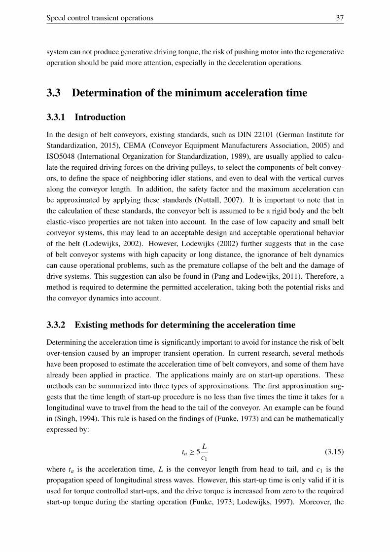
Speed control transient operations 37
system can not produce generative driving torque, the risk of pushing motor into the regenerativeoperation should be paid more attention, especially in the deceleration operations.
3.3 Determination of the minimum acceleration time
3.3.1 Introduction
In the design of belt conveyors, existing standards, such as DIN 22101 (German Institute forStandardization, 2015), CEMA (Conveyor Equipment Manufacturers Association, 2005) andISO5048 (International Organization for Standardization, 1989), are usually applied to calcu-late the required driving forces on the driving pulleys, to select the components of belt convey-ors, to define the space of neighboring idler stations, and even to deal with the vertical curvesalong the conveyor length. In addition, the safety factor and the maximum acceleration canbe approximated by applying these standards (Nuttall, 2007). It is important to note that inthe calculation of these standards, the conveyor belt is assumed to be a rigid body and the beltelastic-visco properties are not taken into account. In the case of low capacity and small beltconveyor systems, this may lead to an acceptable design and acceptable operational behaviorof the belt (Lodewijks, 2002). However, Lodewijks (2002) further suggests that in the caseof belt conveyor systems with high capacity or long distance, the ignorance of belt dynamicscan cause operational problems, such as the premature collapse of the belt and the damage ofdrive systems. This suggestion can also be found in (Pang and Lodewijks, 2011). Therefore, amethod is required to determine the permitted acceleration, taking both the potential risks andthe conveyor dynamics into account.
3.3.2 Existing methods for determining the acceleration time
Determining the acceleration time is significantly important to avoid for instance the risk of beltover-tension caused by an improper transient operation. In current research, several methodshave been proposed to estimate the acceleration time of belt conveyors, and some of them havealready been applied in practice. The applications mainly are on start-up operations. Thesemethods can be summarized into three types of approximations. The first approximation sug-gests that the time length of start-up procedure is no less than five times the time it takes for alongitudinal wave to travel from the head to the tail of the conveyor. An example can be foundin (Singh, 1994). This rule is based on the findings of (Funke, 1973) and can be mathematicallyexpressed by:
ta ≥ 5Lc1
(3.15)
where ta is the acceleration time, L is the conveyor length from head to tail, and c1 is thepropagation speed of longitudinal stress waves. However, this start-up time is only valid if it isused for torque controlled start-ups, and the drive torque is increased from zero to the requiredstart-up torque during the starting operation (Funke, 1973; Lodewijks, 1997). Moreover, the

38 Energy Saving for Belt Conveyors by Speed Control
applications of Equation 3.15 may result in a steep acceleration ramp and a high peak tensionduring starting (Singh, 1994; Lodewijks, 1997).
To reduce the risk of belt over-tension during starting, Singh (1994) introduced a rule ofthumb to approximate the acceleration time. The rule is “one minute per km of conveyorlength”. According to Singh (1994), this rule generally yields satisfactory results. However,if the rule applies to the conveyor whose length exceeds 2 to 3 km, the time length of start-ing procedure may be unnecessarily long, so that the belt dynamic analysis is suggested to becarried out to determine an acceptable start-up time (Lodewijks, 1997).
Lodewijks (1997) proposed a more accurate method estimating the start-up time. In thisapproximation, it is assumed that the conveyor speed is controlled by a static power converter,and that the speed increases linearly. So the acceleration of the belt on the drive pulley isconstant. Then based on Euler-Eytelwein formula (see Equation 3.13), the maximum belt forceof the considered conveyor during stationary operation can be expressed as:
T1,max =
(eµα
eµα −1
)Fd (3.16)
In the case of a long horizontal belt conveyor, the driving force Fd can be calculated by
Fd = C f gL(m′roll +2m′belt +m′bulk
)(3.17)
Then substituting Equation 3.17 into 3.16 yields
T1,max =
(eµα
eµα −1
)C f gL
(m′roll +2m′belt +m′bulk
)(3.18)
In order to accelerate the lump mass of belt, bulk material and idler rolls, an extra force Fac isrequired which can be estimated by
Fac =(m′roll +2m′belt +m′bulk
)La (3.19)
where a is the value of acceleration. The extra drive force yields an extra belt tension T1ac whichapproximates to
T1ac =
(eµα
eµα −1
)Fac (3.20)
Then taking the risk of belt over-tension into account yields the actual minimum safety factor:
SA,min = SB,min
(T1
T1+T1ac
)(3.21)
The substitution of Equations 3.18 and 3.20 into 3.21 gives:
SA,min = SB,min
(1+
aC f g
)−1(3.22)

Speed control transient operations 39
In the case of a belt conveyor with a linear increase of the speed, the belt acceleration is
a =vb
ta(3.23)
Finally, the combination of Equations 3.23 and 3.22 obtains the acceleration time:
ta =vb
C f g
(SA,min
SB,min− SA,min
)(3.24)
Equation 3.24 has been successfully applied to estimate the start-up time of belt conveyors, es-pecially in the cases of horizontal belt conveyors. The applications can be found in (Lodewijks,1997; Nuttall and Lodewijks, 2007). However, it is important to note that, the value resultedby Equation 3.24 normally is larger than the minimum required strat-up time. The deviationmight be caused by the over-estimation of the belt tension. As shown in Figure 3.4, the belttension T1 before the drive pulley equals the tension T2 after the drive pulley adding the drivingforces. In addition, the increase of belt tension T1ac equals the extra driving force Fac. There-fore, the extra belt tension can be overestimated by Equation 3.20. In addition, Equation 3.21is lack of accuracy since the actual belt rating in practice may be far larger than that calculatedby Equation 3.2. Therefore, Equation 3.24 results in a large but safe start-up time. Due to theoverestimation, Equation 3.24 can be applied to calculate the start-up time of conveyors with alimited inclination angle. This is confirmed by He et al. (2016a).
From the above description on these three methods, it is clear that these methods can notbe directly applied to determine the minimum acceleration time of the transient operations.However, the method proposed by Lodewijks (1997) provides an inspiration for the proposal ofthe Estimation-Calculation-Optimization (ECO) method.
3.3.3 ECO Method
The ECO method derives from the approach proposed by Lodewijks (1997). It is based onsimulations and accounts for the dynamic performance of belt conveyors in transient operationsunder speed control. The ECO method consists of three steps: Estimation, Calculation andOptimization. In the Estimation step, an estimator is built to compute the permitted maximumacceleration and initialize the acceleration time. Taking the potential risks caused by impropertransient operations into account, the estimator considers the belt as a rigid element, and com-putes the permitted maximum acceleration in transient operations statically. Then accountingfor the acceleration profiles, the demanded minimum speed adjustment time can be rough esti-mated. Section 3.4 describes the estimation in detail.
The purpose of the Calculation step is to detect whether the potential risks occur in transientoperations with the estimated acceleration time. This step accounts for the effect of belt dynam-ics and hysteresis. The dynamic behavior in transient operations is analyzed by simulations.The simulations are based on an existing finite element model, which has been widely appliedin practice. Section 3.5 gives a detailed description of the dynamic analysis.
With respect to belt viscous-elastic properties, belt performance in transient operations is

40 Energy Saving for Belt Conveyors by Speed Control
complex. The transient operation with the estimated acceleration time may result in, for in-stance, the risk of belt over-tension. In such cases, optimizations are required to improve thedynamic performance and to achieve the minimum acceleration time, which results in healthytransient operations. Section 3.6 details the optimization.
3.4 Estimation- static computation
Taking the potential risks in transient operations into account, an estimator is built in this stepto compute the permitted maximum acceleration. In order to describe the estimator clearly, acase as shown in Figure 3.9 is exampled. The belt conveyor is installed with an inclined angleδ and driven by a head pulley. In order to provide a pre-tension, a single sheave gravity take-updevice with mass MT is mounted at the return side after the head pulley. In the following, boththe permitted maximum acceleration and the permitted maximum deceleration are computed.
MT
L
LS
α
Figure 3.9: An inclined belt conveyor with a single sheaved gravity take-up.
3.4.1 Maximum acceleration
With respect to the risk of belt breaking at the splice caused by over-tension, the belt tensionalong the conveying route must be maintained in a safe level. In cases as shown in Figure 3.9,the maximum belt tension generally occurs right before the drive pulley. The tension T1 insteady state before the drive pulley can be approximated by
T1 = T2+Fd (3.25)
where Fd is the driving force and T2 is the belt tension after the drive pulley. As shown inFigure3.9 where the conveyor is tensioned by a single sheave gravity take-up device, if thedistance between the gravity take-up and the drive pulley is small, the belt tension T2 after thedrive pulley can be approximated by
T2 =12
MTg (3.26)
According to Equation 3.1, the permitted belt tension before the drive pulley can be estimatedby

Speed control transient operations 41
T1,max =kN B
SA,min(3.27)
where B is the belt width. Then the combination of Equations 3.25 to 3.27 yields the maximumpermitted driving force
Fd,max,tensioin =kN B
SA,min− 1
2Mg (3.28)
with respect to the belt over-tension risk.
Belt slippage is another major risk in the acceleration operations. As stated by Euler (1762)and Entelwein (1832), if the driving force exerted on the drive pulley attempts to exceed theavailable frictional forces, the belt will slip around the drive pulley. Then according to Equation3.14, the maximum driving force is
Fd,max,slip = Ff ,max = T2 (eµα −1) (3.29)
with respect to the belt slippage risk.
The rated motor torque is the maximum continuous torque available at the design speed thatallows the motor to do work without overheating. In the practical acceleration operations, themaximum service torque is allowed to be slightly larger than the rated torque Tmotor,nom for fewseconds. The ratio of the maximum service torque and the rated torque is defined as servicefactor (is f ). For example, the standard service factor for an open drip-proof motor is 1.15 in(Emadi, 2004). Then in the acceleration operation, the permitted motor service torque Tmotor,max
isTmotor,max = is f Tmotor,nom (3.30)
and the maximum driving force Fd,max,heat onto the drive pulley is
Fd,max,heat = ir fTmotor,max
Rd=
ir f is f Tmotor,nom
Rd(3.31)
in which ir f is the gearbox reduction ratio and Rd is the drive pulley’s radium.
Then taking these three risks in acceleration operations into account, the permitted maxi-mum driving force Fd,max in transient operations is
Fd,max = min(Fd,max,tension,Fd,max,slip,Fd,max,heat
)(3.32)
As described by Newton’s Second Law, the acceleration is the net result of any and all forcesacting on belt conveyors. Then in acceleration operations, the permitted acceleration is
aac,max =Fd,max −Ff
m(3.33)
where Ff is the total motional resistances, and m is the total lump mass of the belt, rollers andthe bulk material on the belt. According to the standard DIN 22101, the motional resistancealong the conveying route can be estimated by

42 Energy Saving for Belt Conveyors by Speed Control
Ff = C f gL(m′roll +
(2m′belt +m′bulk
)cosθ
)+m′bulkgH (3.34)
and the total mass is
m = L(m′roll +2m′belt +m′bulk
)(3.35)
Finally, the maximum permitted acceleration can be estimated by substituting Equations3.34 and 3.35 into Equation 3.33.
3.4.2 Maximum deceleration
In a soft deceleration operation, the driving force exerted on drive pulleys decreases graduallyand the conveyor speed is reduced smoothly. Differing from the acceleration operation, thedeceleration operation mainly considers the risk of pushing the motor into the regenerativeoperation. In the case of belt conveyors which can not provide the negative driving forces, themaximum deceleration can be estimated by:
ade,max =−Ff
m(3.36)
3.4.3 Speed adjustment time
Acc
eler
atio
n [m
/s2]
Acceleration operation
Spe
ed [m
/s]
Time [s]
Deceleration operation
Figure 3.10: Acceleration profiles and speed curves in the transient operation
The speed adjustment time is the time required in acceleration or deceleration operations,and its value is dependent on the planned acceleration profile. Conventionally, the linear accel-eration was widely applied in start-up operations. However, due to the sudden change of theacceleration at the beginning and the ending of transient operations, the linear acceleration op-erations result in a large mechanical jerk. In order to reduce the mechanical jerk and to enablea soft-start operation, Harrison (1983) recommended a sinusoidal acceleration profile as shownin Figure 3.10. The figure includes the curves of an acceleration operation and of a decelerationoperation. Mathematically, the acceleration and the speed can be expressed:
a (t) = π
2∆v
tasin
πtta
(3.37)

Speed control transient operations 43
v (t) = v0+∆v
2
(1− cos
πtta
)(3.38)
where ∆v is the speed adjustment range, ta is the speed adjustment time, t is the instantaneoustime (0 ≤ t ≤ ta), and v0 is the original speed before the transient operation. According toEquation 3.37, the maximum acceleration occurs at t = ta/2 and
amax = a( ta
2
)=π
2∆v
ta(3.39)
Then in transient operations with sinusoidal acceleration profiles, the required minimum speedadjustment time is
tac,min =π
2∆v
aac,max(3.40)
tde,min =π
2∆v
ade,max(3.41)
where the subscripts ac and de represent the operations of the acceleration and deceleration,respectively.
3.5 Calculation- dynamic analysis
In the Estimation step, an estimator is used to approximate the permitted acceleration and thedemanded adjustment time. The estimator views the belt as a rigid element, and assumes that allmasses are accelerated or decelerated at the same time with the same rate. However, Lodewijks(2002) suggests that the neglect of belt elasticity in high capacity and/or long distance conveyorsmay lead to operational problems, for instance premature collapse of the belt and the destructionof pulleys. Moreover, the estimator fails to account for the risk of material spillage caused bythe low speed or by the low belt tension. Therefore, the dynamic analyses play an importantrole when detecting whether the potential risks are prevented in transient operations.
Historically, finite element models of belt conveyor systems have been developed to cal-culate the conveyor dynamic behavior, especially during staring and stopping. Although thesemodels only determine the longitudinal response of the belt by mainly using truss like elements,they have been successful in predicting the elastic response of the belt during starting and stop-ping. An important case study is given by Lodewijks and Kruse (1998) in which both the fieldmeasurements and the finite-element-model-based simulations are carried out. The experimen-tal results show that the deviation between the measured results and the calculated results couldbe restricted within 5%, which falls within the accuracy of the field measurements. Therefore,the finite element model, accounting for the belt elasticity, is capable of analyzing the conveyordynamics in transient operations.
The finite element model of (Lodewijks and Kruse, 1998) is derived from Lodewijks (1996).In the finite element approach, the distributed mass of the belt, the idler rolls and the bulkmaterial is divided into finite number of elements. In Figure 3.11, these elements are presented

44 Energy Saving for Belt Conveyors by Speed Control
by nodes and numbered in sequence. In addition, due to the belt viscosity-elasticity, the adjacentnodes are coupled by a spring-damping connector, presented by a spring element in Figure 3.11.
1234i i-1 i-2
i+2 i+3 i+4NN-1N-2N-3i+1
Figure 3.11: Lump-mass spring-dampened finite element method
12iN N-1
1/2Mg
Fd
1/2Mgx
Figure 3.12: One dimensional model of belt conveyor system.
As Lodewijks (1996) suggests, it is reasonable to suppose that the belt is laid in a horizontaldirection and moves towards one direction. Figure 3.12 illustrates the one dimensional modelof a single drive belt conveyor system. In this model, the driving force Fd is placed on the 1st
node and the pre-tension is placed on both the 1st and N th nodes. The displacement of all nodescan be expressed relative to the displacement of N th node. Then according to Newton’s SecondLaw, the motion of a belt conveyor can be described as
Mx+Cx+Kx = F (3.42)
where
M mass matrix, size N ×N
C matrix of damping factors, size N ×N
K matrix of spring factors, size N ×N
x vector of nodal displacement, size N ×1
Ûx vector of nodal velocity, size N ×1
Üx vector of nodal acceleration, size N ×1
F vector of force, size N ×1
3.6 Optimization- dynamics improvement
With respect to the belt elasticity-viscosity, the dynamic performance of the belt conveyor iscomplex. Due to the fact that the estimator views the belt as a rigid object, the conveyor transient

Speed control transient operations 45
operation in the Calculation step might result in, for instance, the risk of belt slippage. If so,further studies must be carried out to improve the conveyor dynamic performance in transientoperations (He et al., 2016b). Table 3.2 summarizes some solutions, including replacing a newbelt with higher tension rating, optimizing the mass of the take-up device, applying a softerdeceleration profile and increasing the speed adjustment time. With respect to the fact thatchanging the construction or components of an existing conveyor is not practical to some extent,the general method of improvement is to extend the speed adjustment time. Then the third step,Optimization, is carried out to find the minimum speed adjustment time.
Table 3.2: Potential risks in transient operations and their solutions
Potential risks Suggested solutions
Belt over-tension at the splicing areaReplace a new belt with higher tension ratingExtend the speed adjustment time or apply a softeracceleration profileDecrease the mass of take-up devices
Belt slippage around the drive pulleyIncrease the mass of take-up deviceIncrease the wrap angle or replace a new pulleywith a higher friction resistance coefficientExtend the speed adjustment time and reduce thedriving force
Motor overheat
Extend the speed adjustment time and reduce thedriving forceReduce the frequency of speed regulation processReplace a new motor with higher torque ratingInstall a cooling device
Material spillage away from belt Reduce the mechanical jerk by extending speedadjustment time or applying a softer decelerationprofile
Pushing motor into the regenerativeoperation
Apply a softer acceleration profile or extend speedadjustment time
The optimization is realized by using finite-element-model-based simulations. The optimiz-ing procedure can be viewed as a process of root finding. Taking the risk of belt slippage forinstance. The maximum available frictional resistances between the belt and the drive pulley isFf ,bd . It is assumed that during the transient operations, the driving force can exceed the max-imum available friction Ff ,bd . It is further assumed that Fd(t) represents the maximum drivingforce over different acceleration time t. For instance Fd(30) represents the maximum drivingforce during a specific transient operation within the acceleration time 30s. Then with respectto the risk of belt slippage, the minimum acceleration time can be approached by finding theroot of function
f (t) = Fd(t)−Ff ,bd = 0 (3.43)
In spited of the fact that the computer nowadays is very powerful and can quickly complete thecalculations, iteration methods are highly suggested to find the solutions more quickly. These

46 Energy Saving for Belt Conveyors by Speed Control
methods mainly include the bisection method, the false position method, the Newton-Raphsonmethod and the secant method. Because the research of iteration methods is beyond the scope ofthis thesis, the iteration methods will not be further discussed here. More details of the iterationmethods can be found in (Press et al., 1987; Phillips and Taylor, 1996; Pal, 2009).
3.7 Case study: a long horizontal belt conveyor
In order to show how the ECO method is used to determine the minimum acceleration/decelerationtime, this section studies a long horizontal belt conveyor. The belt conveyor is designed byLodewijks (1996). The designed capacity is 2500t/h for conveying coal with density 850kg/m3,and the conveying distance is 1000m. A fabric belt, with Young’s modulus of 370MPa andtension rating of 500kNm, is selected. The linear density of the belt is 14.28kg/m. The car-rying part of the belt is supported by three-roll idler stations with average mass per unit length14.87kg/m. The return part is supported by one-roll idler stations with average mass per unitlength 7.72kg/m. The conveyor is driven by a 250kW motor with torque rating 1592Nm. Moreparameters of the belt conveyor system are illustrated in Table 3.3. As examples of the casestudy, an acceleration operation from 2m/s to 4m/s and a deceleration operation from 4m/s to2m/s are studied in sub-sections 3.7.1 and 3.7.2, respectively.
3.7.1 Acceleration operation from 2m/s to 4m/s
3.7.1.1 Step 1: Estimation
On the basis of data in Table 3.3, Equation 3.28 suggests that the permitted driving force is
Fd,max,tension =kN B
SA,min− 1
2Mg = 86.3kN (3.44)
with respect to the risk of belt over-tension. Taking the risk of belt slippage around the drivepulley into account, Equation 3.29 yields the permitted driving force
Fd,max,slip =12
Mg (eµα −1) = 49.6kN (3.45)
In addition, with respect to the risk of motor over-heating, the maximum driving force is ap-proximated by Equation 3.31:
Fd,max,heat =ir f is f Tmotor,nom
Rd= 54.9kN (3.46)
Then taking these three risks into account, the permitted maximum driving force is
Fd,max = min(Fd,max,tension,Fd,max,slip,Fd,max,heat
)= 49.6kN (3.47)
The result in Equation 3.47 suggests that in acceleration operations of this specific beltconveyor system, the highest risk is the belt slippage around the drive pulley. Moreover, itfurther suggests that due to the phenomenon of belt slippage, both the risk of belt over-tension

Speed control transient operations 47
Table 3.3: Parameters of a coal conveying system with a textile belt. Courtesy of Lodewijks(1996).
Parameters (symbol, unit) value Parameters (symbol, unit) valueConveyor length (L, m) 1000 Mass of bulk material on the belt
per unit length (m′bulk , kg/m)133.54
Nominal capacity (Qnom, MTPH) 2500 Mass of gravity take-up device(mT , kg)
5060
Nominal speed (vnom, m/s) 5.2 Friction coefficient between drivepulley and conveyor belt (µ, −)
0.35
Belt width (B, m) 1.200 Wrap angle of the belt on thedrive pulley (α, °)
180
Young’s modulus of belt (Eb,N/mm2)
340 Motor torque rating (Tnom,motor ,Nm)
1592
Damping factor (D f , −) 0.35 Motor service factor (is f , −) 1.15Cross section area of belt (Abelt ,m2)
0.01236 Reduction factor of gearbox (ir f ,−)
18
Nominal rupture force of belt perunit width (kN , kN/m)
500 Minimal safety factor in steadystate operation (SB,min,−)
8.0
Mass of belt per unit length(m′belt , kg/m)
14.28 Minimal safety factor in transientoperation (SA,min,−)
5.4
Mass of idler per unit length onthe carrying side (m′roll,c, kg/m)
14.87 Coefficient of secondaryresistances (C, −)
1.09
Mass of idler per unit length onthe return side (m′roll,r , kg/m)
7.72 Artificial friction coefficient ( f , -) 0.018
Total mass of idler per unit length(m′roll , kg/m)
22.59
and the risk of motor over-heating are prevented. Then taking the motional resistances alongthe conveying route into account, Equation 3.33 yields the permitted acceleration in accelerationoperations
aac,max =Fd,max −C f gL
(m′roll +2m′belt +m′bulk
)L
(m′roll +2m′belt +m′bulk
) = 0.076m/s2 (3.48)
Accordingly, the minimum acceleration time is initialized as
tac,min =π
2∆V
aac,max= 41s (3.49)
to complete the acceleration operation from 2m/s to 4m/s with a sinusoidal acceleration profile.
3.7.1.2 Step 2: Calculation
In this step, simulations are carried out to examine the conveyor dynamic behavior in the accel-eration operation from 2m/s to 4m/s within 41 seconds. Simulations are based on the followingsuppositions:
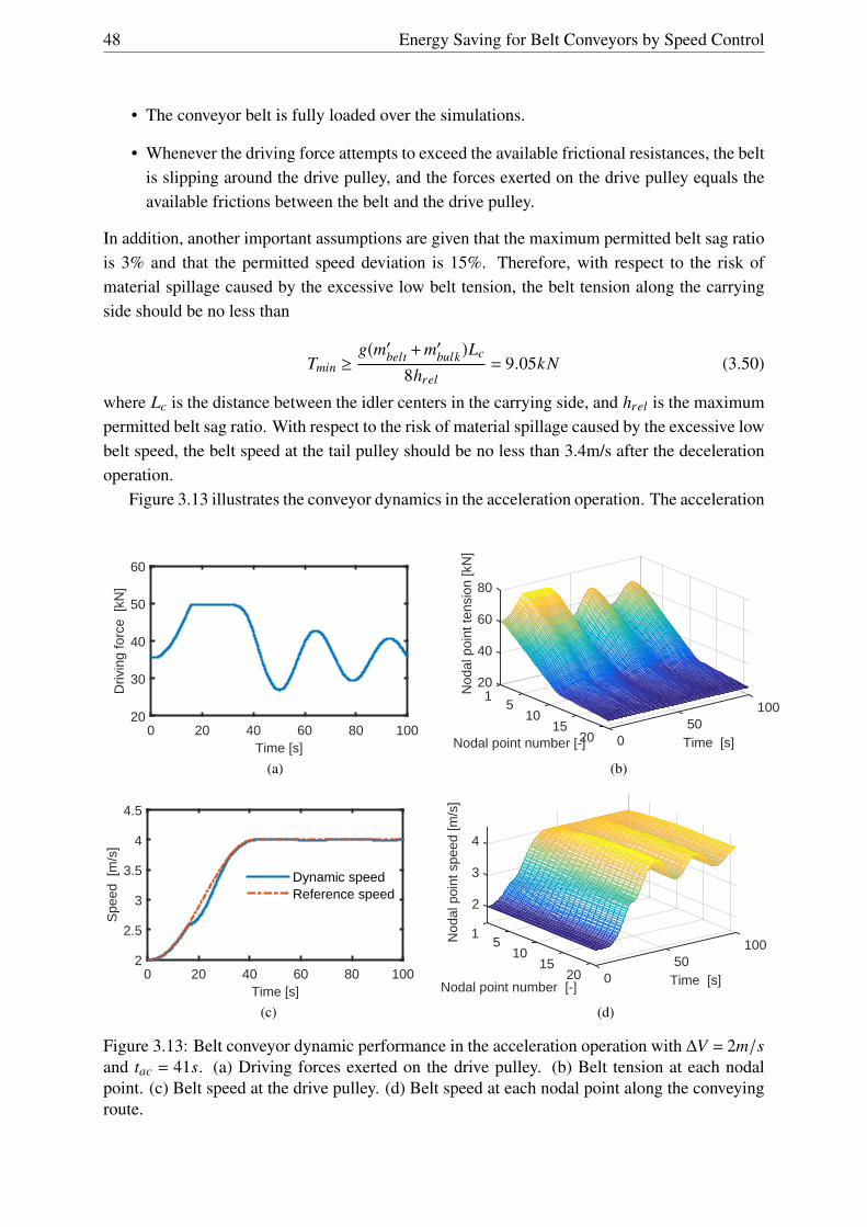
48 Energy Saving for Belt Conveyors by Speed Control
• The conveyor belt is fully loaded over the simulations.
• Whenever the driving force attempts to exceed the available frictional resistances, the beltis slipping around the drive pulley, and the forces exerted on the drive pulley equals theavailable frictions between the belt and the drive pulley.
In addition, another important assumptions are given that the maximum permitted belt sag ratiois 3% and that the permitted speed deviation is 15%. Therefore, with respect to the risk ofmaterial spillage caused by the excessive low belt tension, the belt tension along the carryingside should be no less than
Tmin ≥g(m′belt +m′bulk)Lc
8hrel= 9.05kN (3.50)
where Lc is the distance between the idler centers in the carrying side, and hrel is the maximumpermitted belt sag ratio. With respect to the risk of material spillage caused by the excessive lowbelt speed, the belt speed at the tail pulley should be no less than 3.4m/s after the decelerationoperation.
Figure 3.13 illustrates the conveyor dynamics in the acceleration operation. The acceleration
Time [s]0 20 40 60 80 100
Driv
ing
forc
e [k
N]
20
30
40
50
60
(a)
100
Time [s]50
020Nodal point number [-]15
105
80
20
40
60
1Nod
al p
oint
tens
ion
[kN
]
(b)
Time [s]0 20 40 60 80 100
Spe
ed [
m/s
]
2
2.5
3
3.5
4
4.5
Dynamic speedReference speed
(c)
100
Time [s]50
020Nodal point number [-]
1510
5
2
3
4
1Nod
al p
oint
spe
ed [m
/s]
(d)
Figure 3.13: Belt conveyor dynamic performance in the acceleration operation with ∆V = 2m/sand tac = 41s. (a) Driving forces exerted on the drive pulley. (b) Belt tension at each nodalpoint. (c) Belt speed at the drive pulley. (d) Belt speed at each nodal point along the conveyingroute.

Speed control transient operations 49
starts from the time point 1 second. The diagram of Figure 3.13a illustrates the driving forceexerted on the drive pulley. It shows that at the beginning of acceleration, the driving forceincreases gradually. Around the time point 16 second, the driving force reaches to the limit 49.6kN . Due to the fact that the drive pulley cannot provide more frictional resistances to couplethe exceeding driving forces, the belt is then slipping around the drive pulley and the drivingforce remains at 49.6 kN . The belt slippage continues for 16 seconds, and after that the drivingforce decreases. Due to the belt elasticity, the driving force fluctuates around a certain levelafter the acceleration operation. Meanwhile, due to the belt viscosity, the fluctuation amplitudeis decreasing over time.
Figure 3.13b presents the belt tension at each nodal point. Overall, the diagram shows alongthe carrying side, the minimum belt tension is over 20 kN during and after the accelerationoperation. That means in this acceleration, the risk of material spillage caused by the excessivelow belt tension is avoided. However, the diagram further shows when the belt is slippingaround the drive pulley, an uncontrolled belt tension wave travels from the head pulley to thetail. After that, the belt tension oscillates with dampened amplitudes.
Figure 3.13c shows the dynamic speed curve of the belt around the drive pulley, and the ref-erence speed over time. As the figure shows, the belt speed at the drive pulley gently increasesand follows the reference speed at the beginning of acceleration. However, due to the phe-nomenon of belt slippage, the belt speed at the drive pulley suddenly shocks at the time point 16second. Moreover, due to the fact that the drive pulley can not provide sufficient driving forcesduring the period of belt slippages, the dynamic speed is lower than the reference speed untilthe disappearance of belt slippage. After that, the belt speed at the drive pulley successfullycatches up the reference speed. At the time point 42 second, it finally reaches the desired speed4 m/s. Similar to the driving force, the dynamic speed is fluctuating around the desired speedwith a limited deviation after the acceleration operation.
Figure 3.13d illustrates the belt speed at each node over time. During the acceleration, thebelt speed at each node increases successively. Similar to the belt speed around the drive pulley,the speed curves of other nodes are not thus smooth due to the uncontrolled acceleration wavescaused by belt slippage. In addition, the belt speed is fluctuating with a dampened amplitude fora certain period in response to the belt viscosity-elasticity. Moreover, as is shown the amplitudeof fluctuation of belt speed at the carrying side is less than that at the return side. However, itclear shows that after accelerating, the minimum speed of belt at the tail pulley is larger than 3.4m/s. Therefore, the risk of material spillage caused by exceeding speed deviation is avoided.
Overall, taking the conveyor dynamics shown in Figures 3.13 into account, the accelerationoperation from 2 m/s to 4 m/s within 41 seconds is not acceptable. Optimizations are given inthe next section to find the minimum acceleration time.
3.7.1.3 Step 3: Optimization
The excitation of uncontrolled belt tension waves and of uncontrolled acceleration waves arecaused by the phenomenon of belt slippage. In order to improve the conveyor dynamics, therisk of belt slippage should be avoided. Taking the belt slippage into account, the problem of

50 Energy Saving for Belt Conveyors by Speed Control
optimizing acceleration time is defined as a problem of finding root of function f (t):
f (t) = Fd,max(t)−49.6 = 0 (3.51)
where an important assumption is given that the driving force can exceed the maximum avail-able friction resistances between the belt and the drive pulley.
In order to reduce the computational time, the secant method is applied. Compared to thebisection method and the false position method, the secant method generally can find the rootfaster. In addition, the secant method is more applicable than the Newton-Raphson, due tothe fact that the derivative of the maximum driving force over time is hardly expressed in amathematical way. In the implementation of the secant method, the two initial time points aret0 = 41s and t1 = 71s. The stopping criterion is the function value f (t) less than 0.1.
Table 3.4: Root finding function of f (t) = Fd,max(t)−49.6 = 0 with the secant method. The stopcriteria is |ε | < 0.1.
t1 t2 t3 f (t1) f (t2) f (t3)1 41 71 55,01 5,0930 -5,8101 -1,62282 71 55,01 48,81 -5,8101 -1,6228 0,85623 55,01 48,81 50,95 -1,6228 0,8562 -0,0732
The experimental results are shown in Table 3.4. As the data shows the secant method costsonly three iterations for finding the minimum acceleration time. The data suggests the optimumacceleration time approaches to 51 seconds. Figure 3.14 presents the examination results of theconveyor dynamics during the execution of the 51 seconds acceleration profile. The diagram ofFigure 3.14a clearly shows during the acceleration, the maximum driving force is 49.5 kN . Itsuggests that the risk of belt slippage is successfully avoided. The diagrams of Figures 3.14b to3.14d also show that in the acceleration, both the tensile force and the speed vary smoothly overtime. From the presented results it can be concluded that the conveyor dynamic behavior in thisacceleration operation is acceptable. The operation accelerating the studied conveyor from 2m/s to 4 m/s requires at least 51 seconds.

Speed control transient operations 51
Time [s]0 20 40 60 80 100
Driv
ing
forc
e [k
N]
20
30
40
50
60
(a)
100
Time [s]50
020Nodal point number [-]15
105
80
20
40
60
1Nod
al p
oint
tens
ion
[kN
]
(b)
Time [s]0 20 40 60 80 100
Spe
ed [
m/s
]
2
2.5
3
3.5
4
4.5
Dynamic speedReference speed
(c)
100
Time [s]50
020Nodal point number [-]
1510
5
2
3
4
1Nod
al p
oint
spe
ed [m
/s]
(d)
Figure 3.14: Belt conveyor dynamics in the acceleration operation from 2 m/s to 4m/s within51 seconds. (a) Driving forces exerted on the drive pulley. (b) Belt tension at each nodal point.(c) Belt speed at the drive pulley. (d) Belt speed at each nodal point along the conveying route.

52 Energy Saving for Belt Conveyors by Speed Control
3.7.2 Deceleration operation from 4 m/s to 2 m/s
3.7.2.1 Step 1: Estimation
Pushing the motor into the regenerative operations is the major risk during the deceleration op-eration. With respect to this risk, the driving torque of the drive pulley should be non-negative.Accordingly, the maximum deceleration is
ade,max = −C f g = −0.19m/s2 (3.52)
Then based on the formula 3.41, the estimated deceleration time is
tde,min =π
2∆V
ade,max= 16.5s ≈ 17s (3.53)
With respect to the risk of material spillage caused by the excessive low belt speed, the beltspeed at the tail pulley should remain over 1.7 m/s after the deceleration operation.
3.7.2.2 Step 2: Calculation
Figure 3.15 illustrates the examination results of the deceleration operation from 4 m/s to 2 m/swithin 17 seconds. Figure 3.15a presents the driving forces exerted on the drive pulley. Thediagram shows at the start of the decelerating procedure, the driving force decreases graduallyover time. Meanwhile, both the belt tension and the belt speed change smoothly, see Figures3.15b and 3.15d respectively. However, the diagram in Figure 3.15a shows at the time point11 second, the driving force reduces to the bottom 0kN, and then the driving forces are lost.This phenomenon continues for about 8 seconds. As Figures 3.15b to 3.15c show, the belttension and speed along the conveyor are uncontrollable during this period. The diagram inFigure 3.15c clearly shows the belt speed at the drive pulley fails to follow the reference speed.Therefore, the deceleration from 4 m/s to 2 m/s within 17 seconds is unacceptable.
Besides the sudden loss of driving force, this deceleration also results in the belt slippagearound the drive pulley. As the diagram in Figure 3.15a shows, at the time point 26 second, thedriving force reaches its traction limit, and then the slippage occurs. The slippage causes anuncontrollable acceleration wave, see Figures 3.15d and 3.15c. As the diagram in Figure 3.15cshows, the slippage results in an unexpected speed deviation. The deviation lasts for around 10seconds.
The diagram in Figure 3.15d also shows a large speed deviation during and after the decel-eration. The largest deviation between the drive and tail pulley can be over 1m/s. The figurefurther shows at the time point 24 second, the tail pulley speed drops to 0.9 m/s, less than halfof the required speed. This phenomenon increases the risk of material spillage away from thebelt at the loading area. Therefore, special attention should be paid to this phenomenon duringthe deceleration operation.
From the presented results in Figure 3.15, it can be concluded that the deceleration activityfrom 4 m/s to 2 m/s within 17 seconds will result in the risk belt slippage, the risk of pushingthe motor into the regenerative operation, and the risk of material spillage. Therefore, the

Speed control transient operations 53
Time [s]0 20 40 60 80 100
Driv
ing
forc
e [k
N]
0
20
40
60
(a)
100
Time [s]50
020Nodal point number [-]
1510
5
100
0
50
1Nod
al p
oint
tens
ion
[kN
]
(b)
Time [s]0 20 40 60 80 100
Spe
ed [
m/s
]
1.5
2
2.5
3
3.5
4Dynamic speedReference speed
(c)
100
Time [s]50
020Nodal point number [-]
1510
5
0
2
4
1
Nod
al p
oint
spe
ed [m
/s]
(d)
Figure 3.15: Belt conveyor dynamic behaviors in the deceleration from 4 m/s to 2 m/s within17 seconds. (a) Driving forces exerted on the drive pulley. (b) Belt tension at each nodal point.(c) Belt speed at the drive pulley. (d) Belt speed at each nodal point along the conveying route.

54 Energy Saving for Belt Conveyors by Speed Control
deceleration operation with estimated deceleration time is not acceptable. Taking these risksinto account, the next step will carry out further simulations to improve the conveyor dynamicsand to find the minimum deceleration time.
3.7.2.3 Step 3: Optimization
The examination results in Figure 3.15 illustrate the existence of the risk of pushing motor intothe generative operation, of the risk of belt slippage and of the risk of material spillage. Takingthe risks into account, the problem of optimizing deceleration time can be defined as:
t∗ = max(t∗f , t∗g, t∗h) (3.54)
in which
t∗f the root of function f (t) = FdA,max(t) − 49.6 = 0 with respect to the risk of beltslippage
t∗g the root of function g(t) = FdA,min(t) = 0 with respect to the risk of pushing motorinto the regenerative operation
t∗h the root of function h(t) = vmin(t) − 1.7 = 0 with respect to the risk of materialspillage caused by the excessive low belt speed.
Similar to the optimization step in the acceleration operation, the secant method is applied herefor finding the roots for functions f (t), g(t) and h(t). Then comparing these roots yields theminimum deceleration time for deceleration operation from 4 m/s to 2 m/s with acceptabledynamic performance. It is important note that in order to implement the secant method, thevalue of the driving force can be either over 49.5 kN or below 0 kN .
Finding the root of function f (t) first. The initial points are 17 and 47, and the stop criteriais |ε | < 0.1. Table 3.5 presents the root finding result. The root is approached after four timesof iterations. The data in Table 3.5 suggests that with respect to the risk of belt slippage, theminimum deceleration time is 30.37 second.
The data in Table 3.5 also includes the function values of g(t) and h(t) at point t3. The dataimplies that the activity of finding root of g(t) can be canceled since when the deceleration timeequals 30.37 seconds, the minimum driving force is far larger than 0kN. However, there stillexists the risk of material spillage when t3 = 30.37s. But the data in the second row clearlyshows the root of function h(t) should near 35.2. Table 3.6 illustrates the root finding resultof function h(t) with initial points 35.2 and 47. The root 35.44 is found after three times ofiterations.
Finally, the optimum deceleration time for the deceleration operation from 4 m/s to 2 m/sis obtained, and equals 35.44 seconds. If we continue round the root to the nearest integerwhich is no less than the root, the minimum deceleration time of this deceleration operationis 36 seconds. Figure 3.16 presents the dynamic performance of the belt conveyor during thedeceleration operation from 4 m/s to 2 m/s within 36 seconds. The figure shows during andafter the execution of the 36 seconds deceleration operation, the driving forces value always stay

Speed control transient operations 55
Table 3.5: Root finding function of f (t) = Fd,max(t)−49.6 = 0 with the secant method. The stopcriteria is |ε | < 0.1. The function values g(t3) and h(t3) are also given.
t1 t2 t3 f (t3) g(t3) h(t3)1 17 47 35,2 -6,4518 12,0559 -0,01092 47 35,2 25,23 8,0495 1,5833 -0,60663 35,2 25,23 30,76 -0,6148 7,9286 -0,24874 25,23 30,76 30,37 -0,0479 7,5258 -0,2719
Table 3.6: Root finding function of h(t) = vmin(t) − 1.7 = 0 with the secant method. The stopcriteria is |ε | < 0.01. The function values f (t3) and g(t3) are also given.
t1 t2 t3 f (t3) g(t3) h(t3)1 35,2 47 35,78 -7,1217 12,5364 0,01632 47 35,78 34,83 -6,0124 11,7427 -0,02883 35,78 34,83 35,44 -6,7318 12,2563 0,0005
Time [s]0 20 40 60 80 100
Driv
ing
forc
e [k
N]
0
20
40
60
(a)
100
Time [s]50
02015
105
80
20
40
60
1
Nod
al p
oint
tens
ion
[kN
]
(b)
100
Time [s]50
020Nodal point number [-]
1510
5
0
2
4
1
Nod
al p
oint
spe
ed [m
/s]
(c)Time [s]
0 20 40 60 80 100
Spe
ed [
m/s
]
1.5
2
2.5
3
3.5
4Dynamic speedReference speed
(d)
Figure 3.16: Belt conveyor dynamics in the deceleration operation from 4m/s to 2m/s within36 seconds. (a) Driving forces exerted on the drive pulley. (b) Belt tension at each nodal point.(c) Belt speed at each nodal point along the conveying route. (d) Belt speed at the drive pulley.

56 Energy Saving for Belt Conveyors by Speed Control
positive but below the friction limit. Meanwhile, both the belt tension and the belt speed alongthe conveying route are varying smoothly. Apparently, this deceleration operation is acceptable.
In the case of belt conveyors with variable material feeding rate, the belt speed is expectedto be regulated accurately to match the varying mass flow. In order to prevent continuous highstress, the conveyor speed is regulated discretely with several specific speeds. For the studiedbelt conveyor, it is assumed that the selected speeds are 2 m/s, 2.5 m/s, 3 m/s, 3.5 m/s, 4m/s, 4.5 m/s, 5 m/s and 5.2 m/s. Using the ECO method, more research is carried out, andFigure 3.17 gives the minimum speed adjustment time, both in acceleration and decelerationoperations.
Desired speed v1 [m/s]
2 3 4 5
Acc
eler
atio
n tim
e t ac
[s]
0
20
40
60
80
v0=5m/s
v0=4.5m/s
v0=4m/s
v0=3.5m/s
v0=3m/s
v0=2.5m/s
v0=2m/s
(a)
Desired speed v1 [m/s]
2 3 4 5
Dec
eler
atio
n tim
e t de
[s]
0
10
20
30
40
v0=5.2m/s
v0=5m/s
v0=4.5m/s
v0=4m/s
v0=3.5m/s
v0=3m/s
v0=2.5m/s
(b)
Figure 3.17: Minimum speed adjustment time for different speed adjustment ranges. (a) Mini-mum acceleration time. (b) Minimum deceleration time.
3.8 Conclusion
This chapter answered the second key research question raised in Chapter 1: How to determinethe permitted maximum acceleration and the demanded minimum acceleration time in transient

Speed control transient operations 57
operations? It proposed the ECO method and a long horizontal belt conveyor was studied.According to the experimental data, an overall conclusion can be drawn: the ECO method isapplicable to determine the minimum speed adjustment time, both in acceleration and decel-eration operations. In addition, the following sub-conclusions can also be drawn based on theexperimental results:
• The finite element method can be used to examine the conveyor dynamic performance intransient operations.
• The transient operations with the initialized acceleration time may result in the risks.
• These risks can be successfully prevented if the optimized speed adjustment time is used.

58 Energy Saving for Belt Conveyors by Speed Control

Chapter 4
Belt conveyor energy model
Chapter 3 discussed the transient operations of a belt conveyor under speed control, and pro-posed the ECO method for determining the minimum speed adjustment time. That improvedthe applicability of belt conveyor speed control. In order to evaluate the economic performanceof speed control, it is worth building a parametric energy model for belt conveyors. This chap-ter discusses the energy model of belt conveyors. Standard DIN 22101 (German Institute forStandardization, 2015) is widely used in practice for estimating the power consumption of beltconveyors. DIN-based energy model is detailed in Section 4.1 in which the artificial frictionalcoefficient f is used to calculate the main resistances of a belt conveyor. Section 4.2 proposestwo ways to achieve the f factor value: physical experiment and analytical calculation. How-ever, physical experiments are expensive in practice and they may have a negative impact onthe production plan. Therefore, the thesis uses the analytical method for determining the ffactor value. The analytical method divides the main resistances into four types of individualresistances and calculates these resistances by using the individual calibrated resistance mod-els. Section 4.3 details the modeling of the sub-resistances and a case is studied in Section 4.4to show the analytical calculation. Taking the power losses of the driving units into account,Section 4.5 discusses the driving system efficiency. Some conclusion remarks of this chapter isgiven in Section4.6.
4.1 DIN-based belt conveyor energy model
In last decades, several energy models have been developed to estimate the power consumptionof belt conveyors. Most of energy models are based on belt conveyor design standards, such asDIN 22101 (German Institute for Standardization, 2015) and ISO 5048 (International Organiza-tion for Standardization, 1989). The thesis uses the DIN-based energy model for estimating thepower consumption of belt conveyors and so that to assess the performance of belt conveyorsunder speed control.
Standard DIN 22101 is proposed by German Institute for Standardization (2015) for calcu-lating and dimensioning belt conveyor components. This standard is widely used in practice forassisting in designing belt conveyors. This section gives a detail of the calculations. German In-stitute for Standardization (2015) suggests that the required mechanical power Pm is determined
59

60 Energy Saving for Belt Conveyors by Speed Control
by the driving forces Fd exerted on the driving pulley(s) and the conveyor belt speed v
Pm = Fdv (4.1)
Then taking the power losses in the driving system into account, the demanded electrical powerPe is
Pe =Pm
ηsys=
Fdv
ηsys(4.2)
in the cases of non-generating belt conveyors. In the steady operating conditions, the drivingforces equal to the total motional resistances Ff along the conveying route
Fd = Ff (4.3)
DIN 22101 divides the total motional resistances into four groups: main resistance FH , sec-ondary resistances FN , gradient resistances FSt and special resistances FS:
Ff = FH +FN +FSt +FS (4.4)
These resistances are individually described below.
4.1.1 Main resistances FH
The main resistances FH , also called primary resistances, are resistances occurring along thewhole length of the conveyor. These resistances consist of belt indentation resistances, belt andbulk material flexural resistances, and rotating resistances of rollers. German Institute for Stan-dardization (2015) indicates that the main resistances can be responsible for up to 90% of thetotal resistances. In order to estimate the main resistances, German Institute for Standardization(2015) further introduces an index of artificial frictional coefficient f , and approximates themain resistances by
FH = f gL[m′roll +
(2m′belt +m′bulk
)cosδ
](4.5)
where
L the conveyor length, m
m′roll the mass of idler rolls per unit length, kg/m
m′belt the mass of belt per unit length, kg/m
m′bulk the mass of bulk solid material on the belt per unit length, kg/m
δ inclination angle of a belt conveyor system, °. In the case of declined belt conveyorsystems, the value of δ is negative.
As German Institute for Standardization (2015) emphasizes, the selection of the artificial fric-tional coefficient is significantly important in the design process of belt conveyors. For the

Belt conveyor energy model 61
cases satisfying the following limiting conditions, German Institute for Standardization (2015)suggests the standard value for the f factor shown in Table 4.1 for estimating the total mainresistances of belt conveyors:
• 3 roller fixed idler sets in the top run
• carrying idlers with anti-friction bearings and labyrinth seals
• values of belt sag ratio less than 1%
• filling ratio within a range from 70% to 110%
Table 4.1: Standard values for the artificial friction coefficient f for estimating the total primaryresistance. Courtesy of the standard DIN 22101 German Institute for Standardization (2015).
Characteristic Values for characteristicInternal friction of the bulk material medium low highBelt conveyor alignment medium good badBelt tension medium high lowOperating conditions (dusty, sticky) medium good badIdler diameter 108 to 159 > 159 < 108Spacing of upper strand idlers in m 1.0 to 1.5 < 1.0 > 1.5Spacing of lower strand idlers in m 2.5 to 3.5 < 2.5 > 3.5Belt speed in m/s 4 to 6 < 4 > 6Troughing angle in ° 25 to 35 < 25 > 35Ambient temperature in °C 15 to 25 > 25 < 15Artificial frictional coefficient f standard value≈0.020 0.010~0.020 0.020~0.040
4.1.2 Secondary resistances FN
Differing from the main resistances existing along the whole conveying route, the secondary re-sistances FN only occur at the head and tail of the systems. German Institute for Standardization(2015) suggests, the secondary resistances are mainly composed of fives parts:
• the inertia resistance of material conveyed and the friction resistance between materialconveyed and the belt in the feeding zone, FAu f ;
• the friction resistance between conveyor belt and lateral chutes in the acceleration zoneof a feeding point, FSchb;
• the friction resistance caused by belt cleaners,FGr ;
• the bending resistance of the conveyor belt where it runs over a pulley, FGb;
• and the resistance of the bearings of non-driven pulleys, FTr .

62 Energy Saving for Belt Conveyors by Speed Control
In the case of belt conveyors where secondary resistances occupy a small proportion in the totalresistance, German Institute for Standardization (2015) introduces the secondary coefficient Cto approximate the total secondary resistances
FN = (C−1)FH (4.6)
German Institute for Standardization (2015) further suggests that, the C factor is dependenton the conveyor length. If the belt filling ratio is in the range from 70% to 110%, Table 4.2illustrates the value of coefficient C over different conveyor lengths.
Table 4.2: Standard values of coefficient C for belt conveyor installations with filling ratiosin the range from 70% to 110%. Courtesy of the standard DIN 22101 (German Institute forStandardization, 2015).
L(m) 80 100 150 200 300 400 500C 1.92 1.78 1.58 1.45 1.31 1.25 1.2
L(m) 600 700 800 900 1000 1500 ≥2000C 1.17 1.14 1.12 1.1 1.09 1.06 1.05
4.1.3 Gradient resistances FSt
When the belt and bulk solid travel uphill or downhill with a slope of δ, the weight of beltand bulk solid can be divided into two components: one perpendicular to the conveying direc-tion which is the major reason of the main resistance FH , and the other along the conveyingdirection which generates the gradient resistance FSt . In the case of inclined or declined beltconveyors, the gradient resistance can be relatively larger than other resistances. German Insti-tute for Standardization (2015) suggests, the gradient resistance can be up to 65% of the totalmotional resistances in the case of a belt conveyor with 5% inclination. Differing from the mainresistances and the secondary resistances, the gradient resistance can be precisely determinedby
FSt = Lm′bulkgsinδ = Hm′bulkg (4.7)
where H is the height difference of the belt conveyor.
4.1.4 Special resistances FS
Special resistances FS generally occur only on specially designed belt conveyor systems. AsGerman Institute for Standardization (2015) and Phoenix Conveyor Belt Systems GMBH (2004)suggest, the special resistances can be caused by
• tilted idler position, which arises the tilting resistance FRst at side carrying idlers
• chutes outside the feeding points, which arise extra chute frictional resistances FSch
• devices for lateral bulk material discharge along the conveying length, which arise scraperresistances FGa

Belt conveyor energy model 63
The total special resistances FS of a conveyor are the sum of the mentioned individual resis-tances. Note again, these individual special resistances do not occur on all belt conveyors. Thentaking the total sum of special resistances FS into account, the total motional resistances of beltconveyors running at steady state can be approximated by substituting Equations 4.5 to 4.7 intoEquation 4.4:
Ff = CL f g[m′roll +
(2m′belt +m′bulk
)cosδ
]+Hgm′bulk +FS (4.8)
Finally, the required electrical power in steady state amounts to
Pe =CL f g
[m′roll +
(2m′belt +m′bulk
)cosδ
]+Hgm′bulk +FS
ηsysv (4.9)
4.2 Calculation of the DIN f factor value
Equation 4.9 has been widely used to determine the magnitude of motor power in the design ofbelt conveyors. In the design of a new through belt conveyor, standard values for the artificialfriction coefficient f can be selected from Table 4.1 to help calculate the required dimensionsand ratings of belt conveyor components. However, it is important to note that the values of the ffactor in Table 4.1 are only for the purpose of estimating the ratings of belt conveyors. Generally,the suggested standard value often overestimates the power consumption to avoid the overloadof the drive system for safety reasons. In addition, the research results of such as (Lodewijks,2011) show that the frictional coefficient f varies with different conveyor parameters, such asthe cover material of a belt. Moreover, Alles (1994) and Hiltermann et al. (2011) suggeststhat the f factor value will change with both belt load and belt speed of a given belt conveyor.Therefore, the calculation of the f factor value is required before the DIN-based energy modelis used for calculating the power consumption of a belt conveyor. Calculations of the f factorvalue can be performed either by field experiments or by theoretical analyses. The experimentalmethod is illustrated in Section 4.2.1 and Section 4.2.2 details the the analytical method.
4.2.1 Experimental method
Hiltermann et al. (2011) proposed an experimental method for calculating the f factor of anexisting belt conveyor. This calculation was done by implementing simple measurements onpower consumption of the concerned belt conveyor. Hiltermann et al. (2011) supposed that theefficiency of the driving system is constant and that the special resistances FS are negligible.Then on the basis of Equation 4.9, the frictional coefficient can be calculated by
f =Peηsys
v −m′bulkgH
CLg[m′roll +
(2m′belt +m′bulk
)cosδ
] (4.10)
The paper (Hiltermann et al., 2011) does not give the detail of the measurement, but thethesis of (Hiltermann, 2008) does. The studied belt conveyor is frequency-controlled, so that

64 Energy Saving for Belt Conveyors by Speed Control
it is possible to manually alter the conveyor speed by changing the output frequency of theinstalled frequency converter. The belt conveyor is driven by three motors. Two motors drivethe main drive pulley and the third drives a secondary drive pulley which nears the main drivepulley. Hiltermann (2008) assumed that the load of these motors is always more or less equal.The input power of the frequency converter of the first motor is recorded by a power clammeter, so that the total power consumption can be obtained by assuming that all motors deliverthe same power.
The material flows deposited onto the belt conveyor is controlled by means of a hopperwith speed-controlled apron feeder. Prior to the measurement, the speed of the hopper con-veyor is fixed for a specific material feeding rate. The actual material flow is monitored by abelt weighing system with a high accuracy. Belt speeds of the studied conveyor can be variedduring operations. Once the belt speed has reached the desired speed and the belt conveyor hasacquired a constant material load over the entire belt length, the data of the actual electricalpower consumption can be collected and recorded.
Measurements were performed at various steady material flows with different belt speeds.Figure 4.1 illustrates the experimental results. Figure 4.1a shows the measured electric drivepower. As the data shows, the power is relatively linearly correlated with the material flow.Moreover, it clearly shows that lower belt speed requires a lower electric drive power at thesame material flow.
Figure 4.1b gives the derived values of the f factor over different material feeding ratesand belt speeds. From the diagram, it can be seen that the average value for the f factor isabout 0.022. With the derived average value, Equation 4.9 was used in (Hiltermann, 2008;Hiltermann et al., 2011) to predict the actual power consumption of the belt conveyor underdifferent operational conditions.
However, it is important to note that Figure 4.1b also indicates that the frictional coefficientvaries with different speeds and loads. Using the average value for the f factor may result inerrors of energy savings by means of speed control. Moreover, this experimental calculationitself is not that accurate. The reasons are twofold. First, Hiltermann (2008) assumed thatthe driving system efficiency is constant so that he only measured the electric power, insteadof the mechanical power. However, experimental results in (ABB, 2000) shows that that thedriving system efficiency varies over loads and speeds. Another reason is that, Hiltermann(2008) assumed that the three motors of the concerned conveyor could equally share the drivingpower, so that he only detected the electric power of one of the three motors, instead of thetotal electric power of these three motors. However, Hiltermann (2008) did not proof that thethree motors provide the same amount of power. The uneven distribution of the driving torqueamong the three motors can result in the error of the calculation. Hereby, taking these tworeasons into account, the experimental calculation is suggested to be improved by measuringthe driving torque by strain gauges, instead of measuring the electric power. Then the f factorcan be calculated by:
f =Pm−m′bulkgH
CLg[m′roll +
(2m′belt +m′bulk
)cosδ
] = ∑nk=1 Tsha f t,kωsha f t,k −m′bulkgH
CLg[m′roll +
(2m′belt +m′bulk
)cosδ
] (4.11)

Belt conveyor energy model 65
(a)
(b)
Figure 4.1: Experimental results. (a) Measured electrical power. (b) Derived friction coefficient.Courtesy of Hiltermann et al. (2011).
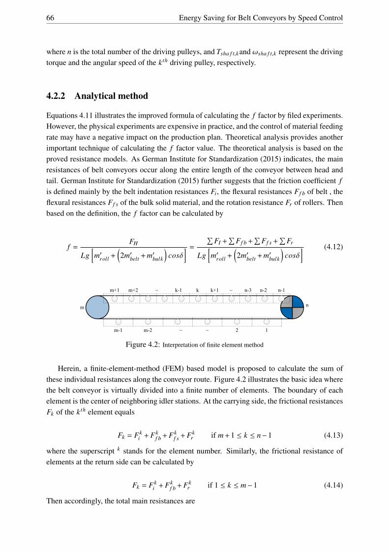
66 Energy Saving for Belt Conveyors by Speed Control
where n is the total number of the driving pulleys, and Tsha f t,kand ωsha f t,k represent the drivingtorque and the angular speed of the k th driving pulley, respectively.
4.2.2 Analytical method
Equations 4.11 illustrates the improved formula of calculating the f factor by filed experiments.However, the physical experiments are expensive in practice, and the control of material feedingrate may have a negative impact on the production plan. Theoretical analysis provides anotherimportant technique of calculating the f factor value. The theoretical analysis is based on theproved resistance models. As German Institute for Standardization (2015) indicates, the mainresistances of belt conveyors occur along the entire length of the conveyor between head andtail. German Institute for Standardization (2015) further suggests that the friction coefficient fis defined mainly by the belt indentation resistances Fi, the flexural resistances Ff b of belt , theflexural resistances Ff s of the bulk solid material, and the rotation resistance Fr of rollers. Thenbased on the definition, the f factor can be calculated by
f =FH
Lg[m′roll +
(2m′belt +m′bulk
)cosδ
] = ∑FI +
∑Ff b+
∑Ff s +
∑Fr
Lg[m′roll +
(2m′belt +m′bulk
)cosδ
] (4.12)
12m-2
m+1 m+2 n-1n-2k k+1k-1~ ~
~~
n
n-3
m
m-1
Figure 4.2: Interpretation of finite element method
Herein, a finite-element-method (FEM) based model is proposed to calculate the sum ofthese individual resistances along the conveyor route. Figure 4.2 illustrates the basic idea wherethe belt conveyor is virtually divided into a finite number of elements. The boundary of eachelement is the center of neighboring idler stations. At the carrying side, the frictional resistancesFk of the k th element equals
Fk = Fki +Fk
f b+Fkf s +Fk
r if m+1 ≤ k ≤ n−1 (4.13)
where the superscript k stands for the element number. Similarly, the frictional resistance ofelements at the return side can be calculated by
Fk = Fki +Fk
f b+Fkr if 1 ≤ k ≤ m−1 (4.14)
Then accordingly, the total main resistances are

Belt conveyor energy model 67
FH =
m−1∑k=1
Fk +
n−1∑k=m+1
Fk =
m−1∑k=1
(Fk
i +Fkf b+Fk
f s +Fkr
)+
n−1∑k=m+1
(Fk
i +Fkf b+Fk
r
)(4.15)
Finally, the f factor can be calculated by
f =
∑m−1k=1
(Fk
i +Fkf b+Fk
f s +Fkr
)+
∑n−1k=m+1
(Fk
i +Fkf b+Fk
r
)Lg
[m′roll +
(2m′belt +m′bulk
)cosδ
] (4.16)
According to Equation 4.16, the key-point of the analytical approach is to calculate theindividual resistances along the conveyor route. This can be achieved by using proved sub-resistance models from literature. The next section will detail the calculation models of theseresistances.
4.3 Modeling of sub-resistances
4.3.1 Indentation resistance of belt
The belt indentation resistance model is based on May et al. (1959), Spaans (1991) and Lodewi-jks (1995).
When the belt moves over a roller station, the contact region of the belt bottom cover is in-dented by the hard roll(s) due to the belt and load weight. Figure 4.3 illustrates the deformationof the belt where a and b represent the front and rear part of the contact length between beltand roller. Due to the belt elasticity-viscosity, the material requires more time to relax to theoriginal pattern so that the rear contact region length b is smaller than the front contact lengtha. The asymmetrical deformation results in the asymmetrical pressure distribution, shown asFigure 4.3. In such a way, the indentation rolling resistance is generated.
Based on the phenomenon of the asymmetrical pressure distribution, May et al. (1959)provides an indentation resistance model, accounting for the rubber elasticity-viscosity. Mayet al. (1959) assumes that the conveyor belt is lying on the ground and that a hard roller isrolling over the belt bottom cover, see Figure 4.4. May et al. (1959) further assumes that thebelt carcass is a rigid base, and that the cover rubber is a linear visco-elastic material. Whenthe roller is moving over the cover rubber, the material in front of the cylinder is compressed,and the original shape is recovered behind the roller. The rubber elasticity-viscosity results inan asymmetrical contact shape between the belt and the roller. May et al. (1959) describes thecover material by using a Winkler foundation model (see Figure 4.4) to approximate the stresspattern. The Winkler model is composed of an infinite number of independent three-parameterMaxwell models. These Maxwell models can be compressed without affecting their neighbors.May et al. (1959) suggests that the stress distribution between roll and the cover rubber can becalculated by
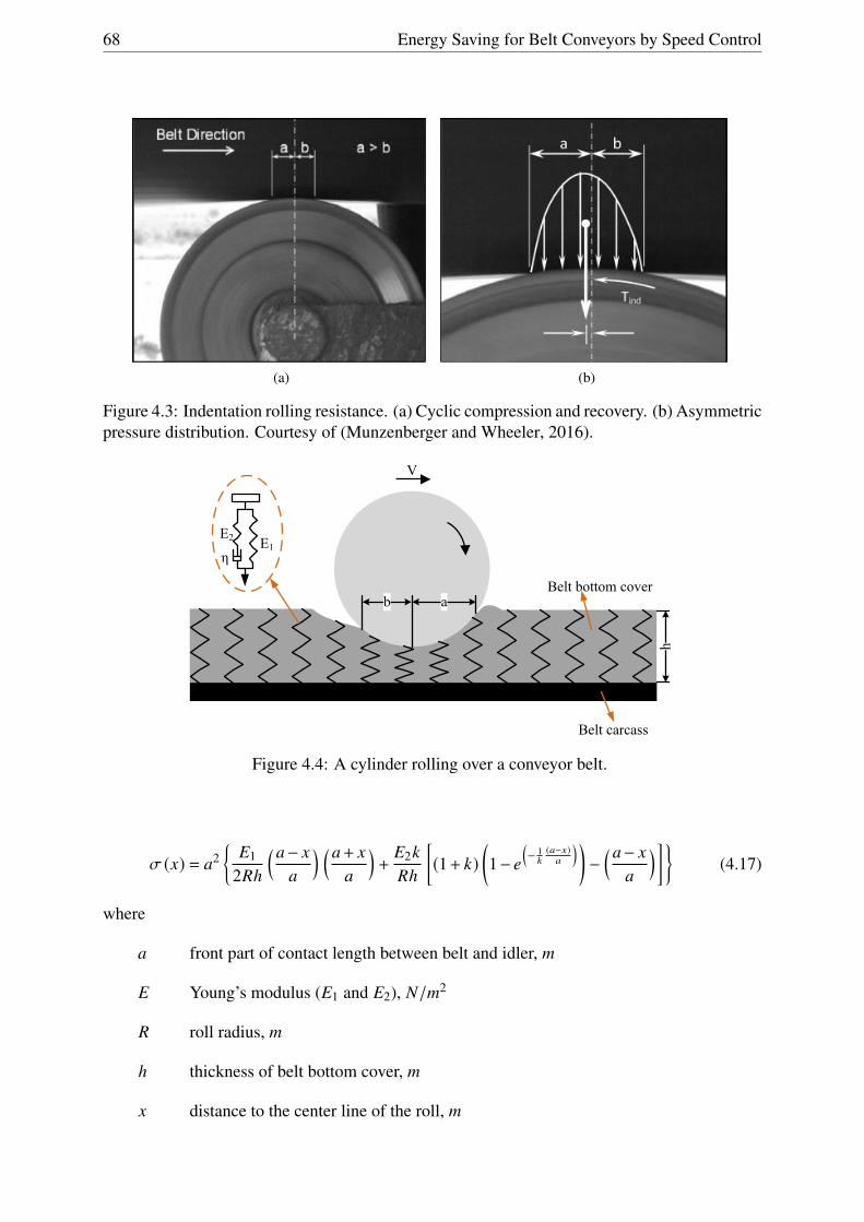
68 Energy Saving for Belt Conveyors by Speed Control
(a) (b)
Figure 4.3: Indentation rolling resistance. (a) Cyclic compression and recovery. (b) Asymmetricpressure distribution. Courtesy of (Munzenberger and Wheeler, 2016).
ab
V
E1E2
η
Belt bottom cover
Belt carcass
h
Figure 4.4: A cylinder rolling over a conveyor belt.
σ (x) = a2{
E12Rh
(a− xa
) (a+ xa
)+
E2kRh
[(1+ k)
(1− e
(− 1
k(a−x)a
) )−
(a− xa
)]}(4.17)
where
a front part of contact length between belt and idler, m
E Young’s modulus (E1 and E2), N/m2
R roll radius, m
h thickness of belt bottom cover, m
x distance to the center line of the roll, m

Belt conveyor energy model 69
k Deborah number, defined by vτ/a, where v is the belt speed and τ is the relaxationtime (τ = η/E2)
If the belt moves at a constant speed v, then the distributed vertical force can be calculated by
F′v =ˆ a
−bσ (x)dx
=E1a3
6Rh
[2−
(ba
)3+3
(ba
)]+
2E2ka3
Rh
[1−
(ba
)2]
(4.18)
where b is the rear part of contact length between belt and idler in m, see Figure 4.4. Derivedfrom Equation 4.18, the contact length a can be calculated by
a =F′v
1/3[E1
6Rh
(2−
(ba
)3+3
(ba
))+
2E2kRh
(1−
(ba
)2)]1/3 (4.19)
Similarly, the total moment M about the center is
M =ˆ a
−bσ (x) xdx (4.20)
Then the total distributed frictional force per unit length is
F′im =MR=
E1a4
8R2h
[1−2
(ba
)2+
(ba
)4]+
E1a4kR2h[
k3− k2
(1+
(ba
)2)+
13
(1+
(ba
)3)− k (1+ k)
(k +
ba
)e−1k ( a+ba )
](4.21)
Calculation result in Equation 4.21 normally underestimates the indentation resistances.As Lodewijks (1995) indicates, May et al. (1959) only considered the normal stress in thematerial, and ignored the shear stresses between adjacent rubber materials, as well as the inertiaof the material. To improve the accuracy of the indentation resistance model, Lodewijks (1995)proposes a correction factor derived from Hunter (1961):
fs =f ∗ihf ∗im
(4.22)
where
fs the correction factor defined by Lodewijks (1995)
f ∗ih the indentation resistance factors derived from the Hunter (1961)
f ∗im the indentation resistance factors derived from the modified May et al. (1959)model

70 Energy Saving for Belt Conveyors by Speed Control
The calculations of these two indentation resistance factors f ∗ih and f ∗im are detailed in (Lodewi-jks, 1995), and the improved estimation is given by
F′i = fsF′im (4.23)
As suggested by Limberg (1988), the indentation rolling resistance could be written as a func-tion of the vertical force and the conveyor speed. Hereby, the indentation resistance can bepresented by
F′i = f(F′v,v
)(4.24)
where f is the function. It is important to note that the result in Equation 4.23 stands for theindentation resistance for unit belt width. To approximate the indentation resistances of a beltover an idler station, it requires to consider the normal force distribution over idler stations. Ifit is assumed that the normal force at a distance x in width to one of belt edges is F′v (x), thenthe total indentation resistance over the idler station can be calculated by
Fi =
ˆ B
0F′i (x) =
ˆ B
0f(F′v (x),v
)(4.25)
In the case of through belt convectors, Spaans (1991) hypothesizes that with respect to theweight of bulk material, the surface pressure on the center roll is evenly distributed and thatthe surface pressure on the covered wing roll section will increase linearly. To calculate thenormal forces acting on the side idler roll of a three-roll idler set, Krause and Hettler (1974)applies a modified version of Coulomb’s earth pressure theory. Krause and Hettler (1974)further suggests that in the coming part of the belt approaching an idler, there is a passivestate of stress in the bulk material. After traveling over the idler, the belt is opening and thestress in the material is in an active state. Then taking both the active and passive stress statesinto account, Krause and Hettler (1974) approximates the normal force on the wing roll by
FNw =14
lρsgl21(Ka +Kp
)cosφw (4.26)
where
ρs density of solid material, kg/m3
l the space of adjacent idler stations, m
l1 width of the belt section on the wing roll, covered by bulk solid materials, m
φw wall friction angle between the belt and the bulk material
Ka the active pressure factor derived from Krause and Hettler (1974)
Kp the passive pressure factor derived from Krause and Hettler (1974)
On the basis of the Coulomb’s earth pressure theory, Krause and Hettler (1974) gives the valuesof pressure factors by

Belt conveyor energy model 71
Ka =
sin (λ+φi)√
sin (λ−φw)+√
sin(φi+φw)sin(φi−β)sin(λ+β)
2
(4.27)
Kp =
sin (λ−φi)√
sin (λ+φw)+√
sin(φi+φw)sin(φi+β)sin(λ+β)
2
(4.28)
where
λ trough angle of the wing roll
φi angle of internal friction of bulk solid material
β angle of repose of bulk solid material
Then taking the total masses of solid materials exerted on a idler set into account, the normalforce on the center roll due to the bulk solid is
FNc = m′bulkgl − 12ρsgal2
1[Kacos (λ−φw)+Kpcos (λ+φw)
](4.29)
Taking both the belt and load weight into account, Figure 4.5 illustrates the surface pressureonto conveyor belt at the carrying side. Diagram in Figure 4.5a virtually divides the belt intofive sections: two uncovered wing sections (A1 and A5), two covered wing sections (A2 andA4), and one center section (A3). As the diagram in Figure 4.5b shows, the normal forcesdistributed on wing rolls at sections A1 and A5 are even. The normal force per width unit onthese two sections is:
F′v (x) = ρbldbgcosλ 0 ≤ x ≤ B1 or B4 ≤ x ≤ B5 (4.30)
where
ρb the belt density, kg/m3
db the belt thickness, m
x the distance in the width direction to the left belt wedge in Figure 4.5b, m
If it is assumed that the normal force along covered wing section increases linearly, then thenormal force on area A2 per width unit is
F′v (x) =2 (x−B1)FNw
BA2+ ρbldbgcosλ B1 ≤ x ≤ B2 (4.31)
As the forces on two wing rolls are symmetric, the normal force on area A4 per width unit canbe calculated by
F′v (x) =2 (B4− x)FNw
BA4+ ρbldbgcosλ B3 ≤ x ≤ B4 (4.32)

72 Energy Saving for Belt Conveyors by Speed Control
A5A1
A2
A3
A4
(a)
x
B1 B2 B3 B4 B5
Fp2,x
Fp1,x
Fp3,x
Fp4,x
Fp5,x
BA2 BA3 BA4BA1 BA5
(b)
Figure 4.5: Surface pressure on a conveyor belt with respect to the weight of bulk solid materialand the weight of the belt. (a) Dividing a belt into five sections. (b) Surface pressure distribution.B1-B5, the distance to the left belt wedge. BA1-BA5, the width of individual belt section.
The surface pressure on the center roll is assumed to be uniform, and then the normal force onthe center roll per width unit is
F′v (x) =FNc
BA3+ ρbldbg B2 ≤ x ≤ B3 (4.33)
Then the Combination of Equations 4.30 to 4.33 gives the weight distribution of belt andthe bulk:
F′v (x) =
ρbldbgcosλ 0 ≤ x ≤ B12(x−B1)FNw
BA2+ ρbldbgcosλ B1 ≤ x ≤ B2
FNc
BA3+ ρbldbg B2 ≤ x ≤ B3
2(B4−x)FNw
BA4+ ρbldbgcosλ B3 ≤ x ≤ B4
ρbldbgcosλ B4 ≤ x ≤ B5
(4.34)
Finally, the substitution of Equation 4.34 into Equation 4.25 gives the belt indentation resis-tance over a three-roll idler station.

Belt conveyor energy model 73
4.3.2 Flexural resistances of belt
The modeling of the flexural resistance of belt is based on the calibrated model of Spaans(1991).
As Spaans (1991) suggested, flexural resistances of belt are caused by the hysteresis lossesof belt under cyclic bendings. Spaans (1991) further suggests that the coefficient of energy lossdue to the belt flexure can be approximated by:
Ψb = ∆M/M (4.35)
where
Ψb energy loss factor due to indentation
M moment, Nm
∆M loss of moment , Nm
Figure 4.6: Transverse and longitudinal stress states. Courtesy of Wheeler (2003).
Considering a piece of belt supported by two rolls, see Figure 4.6. It is assumed that theconveyor belt is evenly loaded and that the load distribution is q with N/m. It is further assumedthat there are two bending curves: one whose center of curvature is at the one directly above theroll, and another one whose center of curvature is at the point of maximum sag. Then accordingto Spaans (1991), the radius of curvatures can be calculated by:
74 Energy Saving for Belt Conveyors by Speed Control
1R1=
Fv
2ωEI− q
T(4.36)
1R2=−qT
(4.37)
where
R1 the radius of curvature over the idler roll, m
R2 the radius of curvature at the point of maximum sag, m
Fv the vertical force due to the weight of the belt and bulk solid refereed to an idlerstation, N
EI the flexural rigidity of the belt, Nm2
q the homogeneous load distribution with respect to the total of the belt and the bulkmaterial, N/m
T the belt tension, N
ω a factor defined by ω =√
T/EI
In (Spaans, 1991), the bending moments are approximated by:
M1 =EI
R1(4.38)
M2 =EI
R2(4.39)
M1 the bending moments occurring within the belt at the point directly above the idlerroll, Nm
M2 the bending moments occurring within the belt at the point of maximum sag, Nm
Then the belt’s flexural resistances can be calculated by:
Ff b = Ψb
(M1R1+
M2R2
)= ΨbEI
(1
R21 +R2
2
)= ΨbEI
[(Fv
2ωEI− q
T
)2+
(−qT
)2]
(4.40)
Spaans (1991) further suggests that, if the conveyor belt is with high tension, Equation 4.40 canbe further reduced to
Ff b =ΨbF2
v
4T(4.41)
Belt conveyor energy model 75
4.3.3 Flexural resistances of solid materials
The modeling of flxural resistances of bulk solid material is based on the calibrated model ofSpaans (1991).
Due to the internal friction of the bulk solid and friction at the belt and bulk solid interface,the flexural resistance of the bulk solid material occurs as a consequence of the belt sag. Spaans(1991) provides an analytical model for calculating the flexural resistance of the bulk solidmaterial due to the longitudinal deformation. As suggested by Spaans (1991), the coefficientof energy loss is a result of the difference between the passive and active stress state when thevolume flow deforms. Spaans (1991) further suggests, if the deformation of the belt is slight,the flexural resistance of the bulk solid material over spacing l can be estimated by
Ff s,l =FvsFv√
TEI
(Kpv −Kav
) d2
12le−ωχ (4.42)
where
Ff s,l flexural resistance of bulk material due to longitudinal deformation
Fvs normal force due to the weight of the material, N
Kav active stress coefficient in a vertical plane
Kpv passive stress coefficient in a vertical plane
χ a horizontal distance from the smallest radius of curvature to the nearest idler, m.The magnitude of the distance depends on the size of trough angle, the belt width,the belt tension and the modulus of elasticity of the carcass.
On the basis of Coulomb’s earth pressure theory, the stress coefficients in a vertical plane arecalculated by:
Kav =1− sinφi
1+ sinφi(4.43)
Kpv =1+ sinφi
1− sinφi(4.44)
Equation 4.42 can be reduced to
Ff s,l =FvsFv√
TEI
4sinφi
cos2φi
d2
12le−ωχ (4.45)
Figure 4.7 illustrates the transverse volume deformation of the bulk material. When thethrough belt opens under the gravity action, the relax of bulk solid forms an active stress statetransversely. Reversely, the closing of the through belt generates a passive stress state. Thetransformation of the stress states also can be found in Figure 4.6. The opening and closingaction occurs over individual half of the idler spacing. It is further assumed that the trough

76 Energy Saving for Belt Conveyors by Speed Control
Figure 4.7: Model of the opening and closing of the trough shape. Courtesy of Spaans (1991).
sides turn over an angle ∆β when the trough shape opens and closes. Then taking the transversedeformation of the trough shape into account, Spaans (1991) provides an analytical model forapproximating flexural resistance Ff s,t of bulk solid material due to the transverse deformation:
Ff s,t =16∆βρsgB3
A2(Kp−Ka
)cosφw (4.46)
However, as Spaans (1991) further suggests, the flexural resistance caused by the opening andclosing of the belt is considerably small, compared to the flexural resistance due to the length-wise deformation of the volume flow. Therefore, it is eligible to ignore the influence of thetransverse deformation in the final calculation of the flexural resistance of bulk solid. Accord-ingly, the final flexural resistance Ff s of bulk solid material can be approximated by
Ff s ≈ Ff s,l (4.47)
4.3.4 Rotating resistances of rollers
The modeling of the rotating resistances of rollers is based on the calibrated models of Lodewi-jks (1995), Wheeler (2003, 2016) and SKF (2016).
Roller shell
Bearing house
Bearing
Roller shaft
Lip seal
Figure 4.8: Roller construction. Courtesy of JLV Industries Pty Ltd (2009).
Figure 4.8 illustrates the major components of a typical roller. A bearing house is amounted
Belt conveyor energy model 77
at each side of the tubing shell. A bearing is assembled into the bearing house to connect ashaft. The bearing house is covered by lip seals to protect the bearing from environmentalpollutants and to keep the bearing house clean. The bearing unit typically is composed ofrolling components, lubricant and seals. When the idler rolls are rotating, the rolling elementsin the bearings cause frictional resistances. Meanwhile, the grease results in energy losses dueto the viscous drag of the lubricant. In addition, the relative rotation between lip seals and thebearing house causes energy losses. According to the definition in SKF (2016), the rotatingresistances Fr of idler rolls can be approximated by
Fr = 2M0+M1+Ms
R(4.48)
where M0, M1, Ms are the friction moments due to the viscous drag of the lubricant, the rollingelements of the bearing and the contact lip seal, respectively.
Lubricants are substances that help to reduce the friction of bearings and to allow smoothmovement. In the case of a grease lubricated bearing, the lubricant frictional moment M0 occursdue to the lubricant’s viscosity property. The lubricant frictional moment is independent of thevertical load but is a function of speed. Moreover, the operating viscosity of the lubricantconsiderably affects the frictional moment M0. In addition, the mean bearing diameter and thewidth of the rolling contact areas also have an effect on M0. In accordance with the experimentalresults, Lodewijks (1995) and Wheeler (2003) approximate the load-independent moment M0
byM0 = 10−1 f0 (νn)2/3 d3
be (4.49)
where
f0 a factor depending on the bearing type and lubrication, in the case of single rowdeep groove ball bearings, f0 = 1.5−2.0
ν the viscosity of lubrication oil, m2s
n the number of rotations per second, s−1
dbe the average bearing diameter, m
The load-dependent friction moment M1 is caused by the sliding resistance and the hysteresisresistance of the bearing elements. Besides the exerted force, the frictional moment M1 alsodepends on the bearing type and the bearing’s mean diameter:
M1 = f1P1dbe (4.50)
where
f1 a load-dependent friction factor
P1 a decisive load for frictional torque, N
78 Energy Saving for Belt Conveyors by Speed Control
Wheeler (2016) indicates that the axial load is considered negligible during operating conditionsin the case of general idler rolls. Therefore the load P1 determining the friction moment canvirtually equal the radial load Fr on the bearing. In addition, Wheeler (2016) suggests that theload-dependent friction factor f1 is considerably varied by the types of bearings. In the case of62 series deep groove ball bearings, the factor is given by
f1 = 0.0008(
P0C0
)0.55(4.51)
while for 63 series deep groove ball bearings
f1 = 0.0009(
P0C0
)0.55(4.52)
where C0 is the static load rating of the bearing given by the bearing manufacturer, and P0 isthe equivalent static bearing load given by
P0 = X0Fr (4.53)
where X0 is the radial factor depending on the bearing design. In the case of sing row deepgrove ball bearings, X0 = 0.6.
Seals are used to to retain the lubricant in the bearing, and to form the closure of bearingsto prevent contaminants from reaching the critical surface inside the bearing. Wheeler (2003)defines these seals as inner seals. Wheeler (2003) further indicates that, the design of the innerlip seal (if present) varies significantly between manufacturers. Different to inner seals, theouter lip seals are used to form the primary boundary of the bearing house to prevent the eternalcontaminants. Wheeler (2003) indicates that the outer lip seals are typically fixed to the shaft,and that the frictional moment of lip seals for idler is approached by
Ms =0.15e25d1s
2πR2 (4.54)
where d1s is the contact diameter of lip seals in m. If grease filled labyrinth seals are requiredto crucially prevent the dust and water into the rolling elements of the bearing, the viscous dragof the grease generates extra frictional moments. The calculation of the frictional moments oflabyrinth seals can be found in (Wheeler, 2003, 2016).
This section has discussed the analytical calculations of the individual resistances along theconveying route. All these calculations are based on the calibrated models from literature. Toshow how the f factor value is achieved by the analytical approach, a fictive long horizontalbelt conveyor will be studied in the next section. The impact of different loads and speeds onthe f factor value also will be discussed.
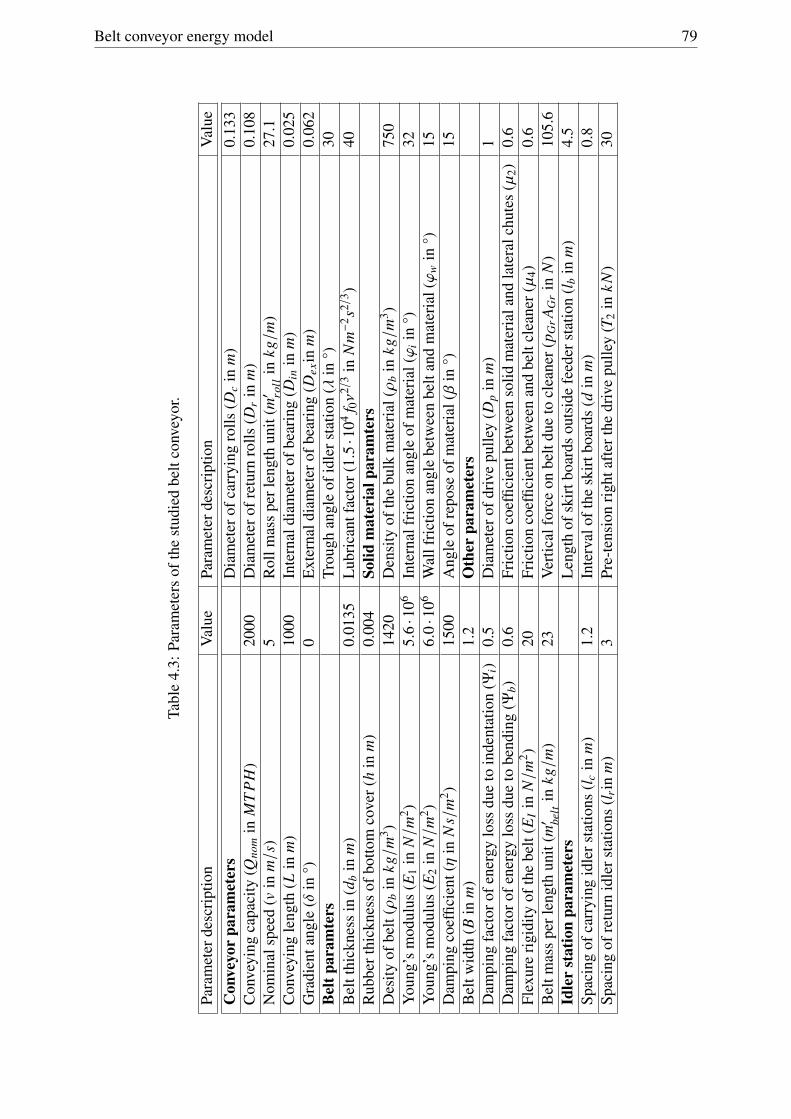
Belt conveyor energy model 79
Tabl
e4.
3:Pa
ram
eter
sof
the
stud
ied
belt
conv
eyor
.
Para
met
erde
scri
ptio
nV
alue
Para
met
erde
scri
ptio
nV
alue
Con
veyo
rpa
ram
eter
sD
iam
eter
ofca
rryi
ngro
lls(D
cin
m)
0.13
3C
onve
ying
capa
city
(Qno
min
MT
PH
)20
00D
iam
eter
ofre
turn
rolls
(Dr
inm
)0.
108
Nom
inal
spee
d(v
inm/s
)5
Rol
lmas
spe
rlen
gth
unit
(m′ ro
llin
kg/m
)27
.1C
onve
ying
leng
th(L
inm
)10
00In
tern
aldi
amet
erof
bear
ing
(Din
inm
)0.
025
Gra
dien
tang
le(δ
in°)
0E
xter
nald
iam
eter
ofbe
arin
g(D
exin
m)
0.06
2B
eltp
aram
ters
Trou
ghan
gle
ofid
lers
tatio
n(λ
in°)
30B
eltt
hick
ness
in(d
bin
m)
0.01
35L
ubri
cant
fact
or(1.5·1
04f 0ν
2/3
inN
m−2
s2/3 )
40R
ubbe
rthi
ckne
ssof
botto
mco
ver(
hin
m)
0.00
4So
lidm
ater
ialp
aram
ters
Des
ityof
belt
(ρb
inkg/m
3 )14
20D
ensi
tyof
the
bulk
mat
eria
l(ρ
bin
kg/m
3 )75
0Y
oung
’ sm
odul
us(E
1in
N/m
2 )5.
6·10
6In
tern
alfr
ictio
nan
gle
ofm
ater
ial(ϕ
iin
°)32
You
ng’s
mod
ulus
(E2
inN/m
2 )6.
0·10
6W
allf
rict
ion
angl
ebe
twee
nbe
ltan
dm
ater
ial(ϕw
in°)
15D
ampi
ngco
effic
ient
(ηin
Ns/
m2 )
1500
Ang
leof
repo
seof
mat
eria
l(β
in°)
15B
eltw
idth
(Bin
m)
1.2
Oth
erpa
ram
eter
sD
ampi
ngfa
ctor
ofen
ergy
loss
due
toin
dent
atio
n(Ψ
i)0.
5D
iam
eter
ofdr
ive
pulle
y(D
pin
m)
1D
ampi
ngfa
ctor
ofen
ergy
loss
due
tobe
ndin
g(Ψ
b)0.
6Fr
ictio
nco
effic
ient
betw
een
solid
mat
eria
land
late
ralc
hute
s(µ
2)0.
6Fl
exur
eri
gidi
tyof
the
belt
(EI
inN/m
2 )20
Fric
tion
coef
ficie
ntbe
twee
nan
dbe
ltcl
eane
r(µ
4)0.
6B
eltm
ass
perl
engt
hun
it(m′ be
ltin
kg/m
)23
Ver
tical
forc
eon
belt
due
tocl
eane
r(p G
rA G
rin
N)
105.
6Id
ler
stat
ion
para
met
ers
Len
gth
ofsk
irtb
oard
sou
tsid
efe
eder
stat
ion
(lb
inm
)4.
5Sp
acin
gof
carr
ying
idle
rsta
tions
(lc
inm
)1.
2In
terv
alof
the
skir
tboa
rds
(din
m)
0.8
Spac
ing
ofre
turn
idle
rsta
tions
(l rin
m)
3Pr
e-te
nsio
nri
ghta
fter
the
driv
epu
lley
(T2
inkN
)30

80 Energy Saving for Belt Conveyors by Speed Control
4.4 Case study of the f factor calculation
4.4.1 Setup
This section performs simulation experiments to show the analytical calculation of the f factorvalue. A long horizontal belt conveyor is studied. Table 4.3 lists the parameters of the concernedconveyor. To simplify the experiments, it is assumed that
• At the carrying side, the conveyor belt is supported by three-roll idler sets with the sametrough angle. The idler sets are evenly distributed along the conveying route. The con-veyor belt is visually divided into L/lc pieces where lc is the idler spacing of the carryingside. The three-roll idler station is in the lengthwise middle of the belt piece.
• At the return side, the conveyor belt is supported by one-roll idler sets and these sets arewith constant pitch. The conveyor belt is evenly divided into L/lr pieces where lr is theidler spacing of the return side. The one-roll idler station is in the lengthwise middle ofthe belt piece.
The case will be studied in which the belt conveyor is running at nominal speed with nom-inal loading rate. Due to the fact that the belt tension has a significant impact on the flexuralresistances, the secondary resistances at the tail pulley are taken into account to improve theaccuracy of the calculation. The separate calculations of the individual secondary resistancesare detailed in DIN 22101 (German Institute for Standardization, 2015).The next section givesthe computational results.
4.4.2 Experimental results
4.4.2.1 Belt indentation resistances
The calculation results of the belt indentation resistances are illustrated in Table 4.4. As thedata shows, at the return side where the belt is empty, the belt indentation resistances over anidler station is 4.87 N . Taking all the idler stations of the return side into account, the total beltindentation resistances are 1.62 kN . At the carrying side, due to the weight of belt and bulk, itrequires 13.88 N to overcome the indentation resistances on a three-roller idler set. The totalindentation resistances of the carrying side are more than 11 kN . Totally, the belt indentationresistances over the whole conveyor are 13.25 kN .
Table 4.4: Belt indentation resistances
Parameter Value Unit
Return side Indentation resistance on an one-roller idler station 4.87 NTotal belt indentation resistances of the return side 1.62 kN
Carrying side Indentation resistances at a three-rollers idler station 13.88 NTotal indentation resistances of the carrying side 11.63 kN
Total (∑
FI) 13.25 kN

Belt conveyor energy model 81
4.4.2.2 Flexural resistances
The flexural resistances includes two parts: the bending losses of the belt and of the bulk solidmaterial. Equation 4.41 suggests that the belt flexural resistances are dependent on the loadand the belt tension. However, due to the fact that the tension difference along the return sideis limited, the difference of belt flexural resistance at the return side is small, see Table 4.5.Differently, the belt tension of the carrying side increases considerably from the tail to the headof the conveyor. Therefore, as the data in Table 4.5 indicates, the belt flexural resistances atthe carrying side are quite different. As the data in Table 4.5 further shows, the total flexuralresistances of belt are around 6.8 kN taking the belt of both the return and carrying sides intoaccount.
Table 4.5: Flexural resistances of belt
Parameter Value Unit(Belt tension right after the drive pulley) 30 kN(Belt tension right before the tail pulley) 34 kNFlexural resistance between neighboring stations minimum 2.02 Nof the return side maximum 2.29 NTotal of the return side 0.71 kN(Belt tension right after the tail pulley) 37 kN(Belt tension right before the drive pulley) 67 kNFlexural resistance between neighboring stations minimum 5.60 Nof the carrying side maximum 10.10 NTotal of the carrying side 6.10 kNTotal (
∑Ff b) 6.81 kN
Table 4.6 illustrates the flexural resistances of the bulk solid material. These resistances onlyexist at the carrying side. From the tail to the head of the conveyor, the load flexural resistancereduces along the conveying route caused by the increase of the belt tension. As the data inTable 4.6 indicates, the maximum of the load’s flexural resistance between neighboring idlerstations can be over 11 N but the minimum is lower to below 7 N . Taking the load distributedalong the whole carrying side into account, the data of Table 4.6 further shows the load’s totalflexural resistances, 7.21 kN .
Table 4.6: Flexural resistances of the bulk solid material
Parameter Value Unit(Belt tension right after the tail pulley) 37 kN(Belt tension right before the drive pulley) 67 kNFexural resistance between neighboring stations minimum 6.96 Nof the carrying side, Ff s maximum 11.17 NTotal (
∑Ff s) 7.21 kN

82 Energy Saving for Belt Conveyors by Speed Control
Table 4.7: Rotating resistance of idler rolls.
Parameter Value Unit
Return sidebottom roll
lubricant friction 0.73 Nbearing rolling friction 0.11 Nlip seal friction 1.65 Ntotal of the bottom roll 2.50 N
total of the one-roll idler stations 0.83 kN
Carrying side
wing roll
lubricant friction 0.52 Nbearing rolling friction 0.03 Nlip seal friction 1.34 Ntotal of the wing roll 1.89 N
center roll
lubricant friction 0.52 Nbearing rolling friction 0.16 Nlip seal friction 1.34 Ntotal of the center roll 2.02 N
total of a three-roll idler station 5.80 Ntotal of carrying side 4.83 kN
Total (∑
Fr) 5.66 kN
4.4.2.3 Rotation resistances
Due to the fact that the belt pre-tension is large, the belt sag has a limited impact on the rotationresistances of idlers. Therefore, it is eligible to study one three-roll idler station of the carryingside and one one-roll idler station of the return side, instead of the whole idler stations. Table4.7 illustrates the individual resistances of the rollers, including the lubricant friction, the bear-ing rolling friction and the lip seal friction. At the return side, the total rotation resistance of theroller is 2.50 N where the lip seal friction occupies up to 1.65 N . Therefore, the lip seal fric-tions make a major contribution to the rotating resistances of rollers of the return side. Similarphenomenon also occurs at the rollers of the carrying side. The idler station of the carrying sidehas three rollers, and the total rotation resistances of a three-roller station are 5.80 N , see Table4.7. Taking all idler stations of the whole conveyor into account, the total rotating resistancesof rollers are 5.66 kN .
4.4.2.4 Final Results
Taking all individual resistances into account, Table 4.8 illustrates the total of main resistances,near 33 kN . Accordingly, the value of the artificial friction coefficient f is calculated by us-ing Equation 4.12. As the data in Table 4.8 shows, the value of the f factor in this case is0.0187, which is in the range from 0.01 to 0.02 suggested by DIN 22101 (German Institute forStandardization, 2015).

Belt conveyor energy model 83
Table 4.8: Total of main resistances in kN and the derived value of the f factor.
Parameter Value UnitTotal indentation resistances (
∑FI) 13.25 kN
Total flexural resistances of belt(∑
Ff b) 6.81 kNTotal flexural resistances of bulk solid (
∑Ff s) 7.21 kN
Total rotation resistances of rollers(∑
Fr) 5.66 kNTotal of main resistances (FH) 32.93 kNThe DIN f factor 0.0187
4.4.3 Further discussion
4.4.3.1 Different speeds and loads
The main resistances are dependent on the belt speed and the load on the conveyor. The ex-perimental results in (Hiltermann, 2008; Hiltermann et al., 2011) show that the value of the ffactor varies over different speeds and loads. To reduce belt conveyor power consumption, theconveyor speed is adjusted to the match the variable material flow. To analyze the power con-sumption and to evaluate the power savings by means of speed control, the DIN-based energymodel will be used in the following chapters. In order to improve the accuracy of the calcu-lation, variable values of the f factor are taken into account. Taking the same concerned beltconveyor for instance. If it is assumed that the minimal conveyor speed is 40% of the nominalspeed, then Table 4.9 illustrates the derived values of the f factor for different filling levels andfor different conveyor speeds. In Table 4.9, the filling ratio ϕ f is the percentage comparisonbetween the actual load and the nominal load on the belt. From the data in Table 4.9, it indi-cates that the f factor varies over loads and speeds. Moreover, it also clearly shows that whenthe conveyor speed is lowered while the loading rate keeps the same, the f factor normally hasan increase. Taking the case where the loading rate is 50% of the nominal for instance. If theconveyor is running at nominal speed, the filling ratio is 50% and the f factor value is 0.0143.However, when the conveyor is running at optimum speed 2.5 m/s, the filling ratio is 100% andthe f factor value increases to 0.0173, see Table 4.9.
4.4.3.2 Non-uniform distribution
In the above experiments, it is assumed that the bulk material on the belt is evenly distributedalong the carrying side. However, in most practical cases, the material feeding rates are varyingover time. Therefore, the lengthwise material distribution normally is non-uniform along theconveyor. In addition, because the relationship between the indentation resistance and the masson the belt is non-linear, the value of the f factor varies with different material flow distribu-tions.
The condition where the conveyor is non-uniform loaded is further studied. Taking the casewhere conveyor is running at nominal speed and the average filling ratio equals 50% for in-stance. A number of simulation experiments are performed. In the experiments, the conveyoris load by a random ratio along the conveying route but the average keeps around 50%. The

84 Energy Saving for Belt Conveyors by Speed Control
Table4.9:T
hecalculated
valuesofthe
ffactorfordifferentspeeds
andfordifferentloads.
VU
010%
20%30%
40%50%
60%70%
80%90%
100%
20.0122
0.01180.0116
0.01170.0119
0.01240.0129
0.01370.0146
0.01550.0166
2.250.0125
0.01200.0119
0.01200.0122
0.01270.0133
0.01400.0149
0.01590.0170
2.50.0127
0.01220.0121
0.01220.0125
0.01300.0136
0.01430.0152
0.01620.0173
2.750.0129
0.01240.0123
0.01250.0128
0.01320.0139
0.01460.0155
0.01650.0175
30.0130
0.01260.0125
0.01260.0130
0.01340.0141
0.01480.0157
0.01670.0178
3.250.0131
0.01270.0127
0.01280.0131
0.01360.0143
0.01500.0159
0.01690.0180
3.50.0132
0.01280.0128
0.01290.0133
0.01380.0144
0.01520.0161
0.01710.0182
3.750.0133
0.01290.0129
0.01300.0134
0.01390.0146
0.01530.0162
0.01720.0183
40.0134
0.01300.0130
0.01310.0135
0.01400.0147
0.01550.0164
0.01740.0184
4.250.0135
0.01310.0130
0.01320.0136
0.01410.0148
0.01550.0165
0.01750.0185
4.50.0135
0.01310.0131
0.01330.0136
0.01420.0148
0.01560.0165
0.01750.0186
4.750.0136
0.01320.0131
0.01330.0137
0.01420.0149
0.01570.0166
0.01760.0187
50.0136
0.01320.0132
0.01340.0137
0.01430.0149
0.01570.0166
0.01760.0187

Belt conveyor energy model 85
experimental results are illustrate in Figure 4.9. The bubbles of the diagram represent the cal-culated f factor values. As the diagram shows, the material distribution of a belt conveyor hasan influence to the f factor. The data in Figure 4.9 shows that the calculated f factor valuesare in the range from 0.0133 to 0.0154. The black line of the diagram stands for the average ofthe calculated f factor values. As it shows, the average f factor value is 0.0143, which exactlymatches the data of Table 4.9. Therefore, it is relatively accurate to use the data in Table 4.9 tocalculate the power consumption of the concerned belt conveyor.
0.012
0.0125
0.013
0.0135
0.014
0.0145
0.015
0.0155
0.016
49.6% 49.9% 50.0% 50.0% 50.1% 50.2%
Mean value of the fillig ratio
Average The f facotr value
Figure 4.9: Derived values of the f factor in the cases of belt conveyors with non-uniformmaterial distribution.
4.5 Drive system efficiency
In Section 4.1, Equation 4.2 calculates the electric power consumption Pe of belt conveyors bydividing the total mechanical power Pm exerted on the driving pulley with the driving systemefficiency ηsys. Sections 4.1 to 4.4 showed the mechanical power calculation by using theDIN-based energy model. This section discusses the power losses along the drive system anddescribes the system efficiency.
Frequency converter Motor Gearbox Pulley
Figure 4.10: Drive system components. The pictures of the components are courtesy of theInternet.

86 Energy Saving for Belt Conveyors by Speed Control
Figure 4.10 illustrates a typical modern drive system of belt conveyors. The drive pulleyof a belt conveyor is driven through a gearbox by an electric motor. The motor is poweredby a frequency converter, and the frequency converter can precisely control the speed and thetorque of the motor. During the power conversion in the motor and the power transmission inthe frequency converter and the gearbox, the driving units are not free of energy losses. In thecases of belt conveyors with a drive system as shown in Figure 4.10, the system efficiency ηsys
can be calculated by
ηsys = η f reqηmotorηgear (4.55)
where
η f req the efficiency of the frequency converter
ηmotor the efficiency of the electric motor
ηgear the efficiency of the gearbox
In the following of this section, the power losses and the efficiency of the driving units will bebriefly discussed.
4.5.1 Frequency converter power losses
Figure 4.11: Source of the frequency converter losses. Courtesy of Aarniovuori et al. (2007).
Figure 4.11 illustrates the sources of the frequency converter losses. As the diagram shows,the losses in the frequency converters are built up from the input choke losses, the rectifier’sconduction losses (diode rectifier), the direct current (DC) link losses, the switching losses ofthe transistors (the IGBT-module in Figure 4.11), and extra losses. The extra losses includethe power consumption of the cooling fan and of the control system. The calculation of theseindividual energy losses can be found in (Aarniovuori et al., 2007) and (Tsoumas et al., 2014).Aarniovuori et al. (2007) further suggests that the transistors are the major source of the fre-quency converter losses. Taking all the losses in the converter into account, the efficiency of theconverter can be calculated by
η f req =Pout
Pin=
Pin−∑
loss f req
Pin(4.56)
where

Belt conveyor energy model 87
Pin the input power of a frequency converter, equalling electric power consumption Pe
consumed by a belt conveyor
Pout the output power of a frequency converter∑loss f req total power loss of a frequency converter
4.5.2 Motor power losses
An electric motor is a machine that converts electric power into mechanical power (Dilshadet al., 2016). The motor input virtually equals the output power of the frequency converter, andit is always larger than the output mechanical power of the motor. The difference between theinput electric power and the output mechanical power is the losses during energy transforma-tion inside the machine. The literature, like (Boglietli et al., 2003) and (Kärkkäinen, 2015),subdivides the motor losses into four groups: copper losses, iron losses, mechanical losses andstray losses. Taking all these individual power losses into account, the motor efficiency can beapproximated by
ηmotor =Pmech
Pelec=
Pelec −∑
lossmotor
Pelec(4.57)
where
Pmech the output mechanical power provided by a motor
Pelec the input electric power of a motor, equal to the output power Pout of the frequencyconverter∑
loss f req total power losses of a motor
4.5.3 Gearbox power losses
In most industrial applications, the gearbox provides gear reduction and torque increase, andthen the output of the gearbox rotates slower but with a higher torque. Michaelis et al. (2011)suggests that the power losses in a gearbox consist of gear, bearing, seal and auxiliary losses(see Figure 4.12). The brief description of the bearing and seal losses can be found in Section4.3.4. Similar to bearing losses, gear losses can be further separated into load-dependent lossesand no-load losses. Fernandes et al. (2015) detail the power losses in gears. Then taking allindividual resistances of the gearbox into account, the gearbox efficiency can be calculated by
ηgear =Pmech,out
Pmech,in=
Pmech,in−∑
lossgear
Pmech,in(4.58)
where
Pmech,out the output mechanical power of the gearbox, equal to the total mechanical powerPm exerted on the drive pulley

88 Energy Saving for Belt Conveyors by Speed Control
Pmech,in the input mechanical power of the gearbox, equal to the output mechanical powerof the motor in Figure 4.10∑
lossgear total power losses of the gearbox, equal to PV in Figure 4.12
Figure 4.12: Composition of gearbox power loss. Courtesy of Michaelis et al. (2011).
4.5.4 Discussion: calculation of the drive system efficiency
Sections 4.5.1 to 4.5.3 briefly discussed the power losses of the driving units and the relativeefficiency. However, the efficiency of the drive units is more used in practice to calculate thefinal electric power consumption. The efficiency of the driving units can be achieved by mea-surements or by consultancy from the drive unit component manufactures. If these driving unitsare connected in a series as shown in Figure 4.10, the final system efficiency can be derivedfrom Equation 4.55.
In order to the simplify the calculation, Hiltermann et al. (2011) and Zhang and Xia (2011)assume that the efficiency of the drive system is constant. However, more experimental resultsshow that the system efficiency is variable over different loads and speeds. Taking frequencyconverters, motors and gearboxes into account, ABB (2000) gives the efficiency of the wholesystem, see Table 4.10. Based on these data, an empirical model can be given that allows thecalculation of the drive system efficiency as a function of the speed ans load ratios:
ηsys (ϕv, ϕT ) = 0.7878+0.1953ϕv +0.05067ϕT −0.1147ϕ2v +0.048ϕvϕT −0.042267ϕ2
T (4.59)
where ϕv and ϕT are the ratio of motor speed and torque, respectively.
Table 4.10: Efficiency of the whole drive system (including the frequency converter, the motorand the gearbox). Courtesy of ABB (2000).
Load ratio ϕτSpeed ratio ϕv 50% 75% 100%
50% 0.884 0.903 0.90675% 0.887 0.911 0.920
100% 0.890 0.913 0.924

Belt conveyor energy model 89
4.6 Conclusion
This chapter described the DIN-based energy model for calculating the power consumptionof belt conveyors. The experimental results showed that the artificial frictional coefficient fwas 0.0187 if the concerned belt conveyor was running at nominal speed with fully loaded.Further simulation results showed that the f factor varied considerably over loads and speeds.Moreover, the experimental data clearly showed that when the conveyor speed was loweredwhile the loading rate kept the same, the f factor had a noticeable increase. Overall, it issuggested to consider the variable value of the f factor to calculate the power consumption of abelt conveyor for different loads and for different speeds.
Based on the DIN-based energy model, the next chapter will describe the modeling of beltconveyor speed controllers. Both the active and passive speed strategies will be described .

90 Energy Saving for Belt Conveyors by Speed Control

Chapter 5
Modeling of speed control systems
As discussed in the previous chapters, researchers and engineers have already studied the beltconveyor speed control for many years. However, these studies mainly focus on the passivespeed control and rarely investigate the active speed control. The performance of speed con-trol can be assessed by field tests or computational simulations. However, field tests are con-siderably more expensive than computational simulations. Therefore, this chapter describesa simulation model of belt conveyor speed control systems for the purpose of analyzing theperformance of speed control, both the active and passive speed control. Before discussingthe modeling of speed controllers, this chapter firstly analyzes the applicability of speed controlsince not all belt conveyor systems can use speed control to reduce power consumption. Section5.2 briefly introduces the scheme of the simulation model which includes two subsystem, theoperational system and the control system. The modeling of the operational system is detailedin Section 5.3, including the process of verification. Section 5.4 discusses the control systemand introduces several different control strategies. The passive and active control strategies areintroduced individually. In addition, the active speed control strategy is further classified intotwo groups: the fixed time interval strategy and the variable time interval strategy. To assess theperformance of speed control, Section 5.5 defines several key performance indicators (KPIs),including the belt conveyor utilization and the power consumption. Lastly, the conclusion ofthis chapter is given in Section 5.6.
5.1 Applicability of belt conveyor speed control
The academic review in Section 2.7 indicated that speed control can reduce the power con-sumption of belt conveyors. Section 2.6 also suggested that a speed control system requires atleast a speed controller, a variable speed drive system and a material flow sensor. However, itis important to note that not all belt conveyor systems can use speed control for the purposeof energy savings, even though these systems are equipped with all above mentioned physicaldevices. Taking a belt conveyor system with a single conveyor for instance. The material feed-ing rate in a certain period must be predicted, either by acknowledging the upstream process ofbulk solid handling system or by knowing the maximum feeding rate of the conveyor feeder.Otherwise, speed control can not be applied, even though the actual material flow onto the belt
91

92 Energy Saving for Belt Conveyors by Speed Control
can be detected in real time. Therefore, the applicability of speed control should be discussedbefore the modeling of belt conveyor speed controller.
The applicability of speed control on the belt conveyor system with a single belt conveyorhas been discussed above. A general rule can be summarized as: the material feeding ratemust be predictable. This rule also can be used on the belt conveyor system with multipleconveyors. Besides the method acknowledging the upstream handling process or the feederfeeding condition, the prediction can also be realized by measurement. In the cases of multiplebelt conveyors in a series, a material flow sensor can be used to detect the material volume/massflow of the upstream belt conveyor in real time. Then taking the speed of the upstream conveyorinto account, the material feeding rate onto the downstream belt conveyor(s) can be predicted.Based on the information of the incoming material flow stream, the speed of the downstreambelt conveyor(s) can be adjusted.
Additionally, the applicability of speed control is also constrained by the actual loading con-dition. Taking the belt conveyor system in different application sites into account, the loadingscenarios can be categorized into four types and the applicability is analyzed as below:
• Scenario 1: constant loading degree in long term operations. In such a scenario, thebulk solid material is loaded onto the belt conveyor with a roughly constant flow duringa long term operation. The material loading degree only changes when one operationis finished or restarted. Such a scenario can be found for instance at an open pit minewhere a skilled operator operates an excavator to continuously load a belt conveyor. Thisscenario can be further categorized into two sub-scenarios as shown in Figure 5.1a. Thesolid line presents the condition in which the feeding rate nears the nominal conveyingcapacity. In these cases, the implementation of speed control will not help in achievinga considerable amount of power reduction, even though we take the active speed controlinto account where the conveyor speed can perfectly match the material flow. The costsof relevant sensors and the controller will be much higher as compared to savings thatcan be achieved in that specific condition. The dashed line in Figure 5.1a presents anthercondition in which the feeding rate is considerably lower than the nominal conveying ca-pacity. In such cases, the passive speed control is strongly suggested. The belt conveyor isrunning at a pre-defined non-nominal speed so that the conveyor is virtually fully loaded.
• Scenario 2: moderately varying loading degree in between long term operations. Thisscenario can be found at a dry bulk terminal where multiple cranes feed a belt conveyor.Each crane produces roughly the same mass flow onto the belt conveyor. In cases wherenot all cranes operate at the same time during different long term operations, the materialloading degree to the same conveyor varies in between two operations. In such cases, theconveyor speed can be reduced to match the number of available cranes.
• Scenario 3: moderately varying loading degree in between short term operations. Com-pared to Scenario 2, some loading scenarios contain roughly constant material flow inbetween operations but the operations vary relatively on short term. For example, thematerial loading patterns of the conveyors in underground long wall mining follow such

Modeling of speed control systems 93
scenario. In such cases, active speed control is suggested so that the conveyor speed canmatch the actual material loading rate.
• Scenario 4: excessively varying loading degree in all operations. In this scenario thefeeding rate changes excessively. This scenario can be considered to be the completelyrandom loading scenario. Although it can be a rare scenario where the nature of the feedflow is absolutely random, similar loading scenarios can be found in underground ironor copper mines. If the conveyor system has only a single belt conveyor, then the ma-terial feeding rate is totally unpredictable. In such cases, speed control is inapplicablefor reducing the power consumption of the single belt conveyor. On the other hand, ifthe conveyor system has multi-conveyors, speed control potentially has the opportuni-ties of energy savings of the downstream belt conveyor(s). However, the frequent speedadjustment may result in considerable stress cycles which may be harmful to the con-veyor system and components. Therefore, in such loading scenarios, speed control is lessapplicable.
Qnom
Time
(a)
Qnom
Time
(b)
Qnom
Time
(c)
Qnom
Time
(d)
Figure 5.1: Types of material loading scenarios. (a) Scenario 1: constant loading degree inlong term operations. (b) Scenario 2: moderately varying loading degree in between long termoperations. (c) Scenario 3: moderately varying loading degree in between short term operations.(d) Scenario 4: excessively varying loading degree in all operations.
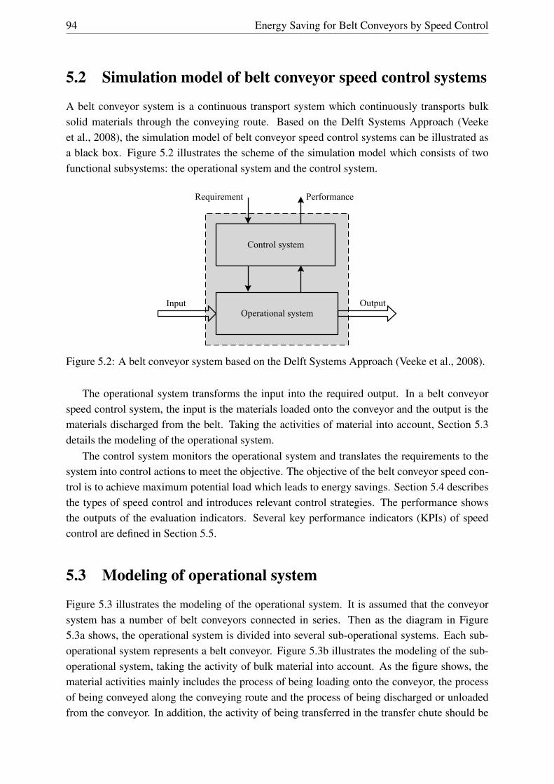
94 Energy Saving for Belt Conveyors by Speed Control
5.2 Simulation model of belt conveyor speed control systems
A belt conveyor system is a continuous transport system which continuously transports bulksolid materials through the conveying route. Based on the Delft Systems Approach (Veekeet al., 2008), the simulation model of belt conveyor speed control systems can be illustrated asa black box. Figure 5.2 illustrates the scheme of the simulation model which consists of twofunctional subsystems: the operational system and the control system.
OutputOperational system
Control system
Requirement Performance
Input
Figure 5.2: A belt conveyor system based on the Delft Systems Approach (Veeke et al., 2008).
The operational system transforms the input into the required output. In a belt conveyorspeed control system, the input is the materials loaded onto the conveyor and the output is thematerials discharged from the belt. Taking the activities of material into account, Section 5.3details the modeling of the operational system.
The control system monitors the operational system and translates the requirements to thesystem into control actions to meet the objective. The objective of the belt conveyor speed con-trol is to achieve maximum potential load which leads to energy savings. Section 5.4 describesthe types of speed control and introduces relevant control strategies. The performance showsthe outputs of the evaluation indicators. Several key performance indicators (KPIs) of speedcontrol are defined in Section 5.5.
5.3 Modeling of operational system
Figure 5.3 illustrates the modeling of the operational system. It is assumed that the conveyorsystem has a number of belt conveyors connected in series. Then as the diagram in Figure5.3a shows, the operational system is divided into several sub-operational systems. Each sub-operational system represents a belt conveyor. Figure 5.3b illustrates the modeling of the sub-operational system, taking the activity of bulk material into account. As the figure shows, thematerial activities mainly includes the process of being loading onto the conveyor, the processof being conveyed along the conveying route and the process of being discharged or unloadedfrom the conveyor. In addition, the activity of being transferred in the transfer chute should be

Modeling of speed control systems 95
taken into account. In the following of this section, the modeling of bulk material activities aregiven individually.
Sub-operational system of BC1
Input Sub-operational system of BC2
Sub-operational system of BCn
Output
Operational system
Control system
(a)
Being loaded onto the conveyor
Being conveyed towards the
conveyor head
Being discharged from
the conveyor
Being transferred in the chute
Sub-Operational system
Input Output
Control system
(b)
Figure 5.3: Modeling of the operational system. (a) Overview of the operational system. Itis assumed that the belt conveyor system has n belt conveyors connected in series. (b) Sub-operational system of each belt conveyor.
5.3.1 Modeling of loading process
If a material flow sensor is installed nearby the loading area, the detected value of material flowrate can be viewed as the real material loading rate in the case of a long belt conveyor. Generally,the data acquisition of the sensor is discrete. If the time interval between adjacent detectingoperations is small, it is acceptable to represent the continuous material loading activity by adiscrete tool.
Figure 5.4 illustrates the discretization of a continuous material loading flow onto a beltconveyor. The diagram in Figure 5.4a shows the real system where the bulk material is continu-ously loaded. The height of the line represents the actual material loading rate of the conveyor.If it is assumed that the conveyor is running at a constant speed and that the sample time isconstant, then the continuous material stream is evenly divided into a finite number of blocksas shown in Figure 5.4b.
The actual material loading rate can vary over time, while a discrete sample is a value at aspecific point in time. Therefore, the real material flow rate between adjacent sampling pointsis unknown. This causes a discretization error whose value depends on the sample rate ofthe flow sensor. Figure 5.5 illustrates the discretization of the loading rate onto the belt withdifferent cycle times. The comparison indicates that if the cycle time is small enough, the

96 Energy Saving for Belt Conveyors by Speed Control
Time
Loading rate
(a)
Time
Loading rateCycle time( )t
(b)
Figure 5.4: Discretization of a continuous material loading flow onto a belt conveyor. (a) Con-tinuous representation of the material loading flow. (b) Discrete representation of the materialloading flow.
Cycle time 2 t
(a)
Cycle time t
(b)
1Cycle time2
t
(c)
Figure 5.5: Comparison between the continuous and discrete representations. (a) Cycle time=2∆t. (b) Cycle time =∆t. (c) Cycle time =1
2∆t.

Modeling of speed control systems 97
discrete representation will be very close to the real continuous system. However, it requiresa lot of computational resources. Therefore, selecting a suitable cycle time is important to themodeling of the material loading flow.
5.3.2 Modeling of conveying process
Drive pulley(s) is continuously rotating to drive the belt conveyor. Due to the friction, it isassumed that bulk material is staying still on the belt so that the material is moving towardthe head of the conveyor with the conveyor speed. Taking the black block in Figure 5.6 forinstance. At the time point t0, the distance between the mass block and the conveyor tail isx (t0), see Figure 5.6a. If it is assumed that the belt speed is v (t0) and then at the time pointt1 = t0+∆t, the traveling distance of the black block in Figure 5.6b can be approximated by
x (t1) = x (t0)+ v (t0)∆t (5.1)
Generally, the belt conveyor system can be treated as a first-in-first-out buffer. Therefore,in terms of other mass blocks as shown in Figure 5.6, the conveying activity can be calculatedseparately.
5.3.3 Modeling of unloading process
It is assumed that the distance between the center lines of the head and the tail pulley is L. Oncethe total traveling distance of a block exceeds the conveyor length, the block is being discharged
v
0x t0x
(a)
v
1 0 0x t x t v t t 0x
(b)
Figure 5.6: Modeling of conveying process. (a) At the time point t0. (b) At the time point t1.
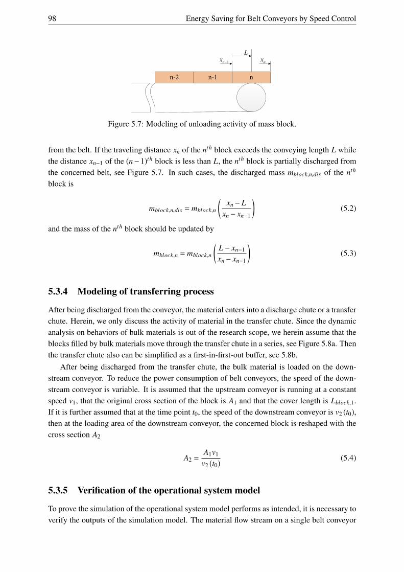
98 Energy Saving for Belt Conveyors by Speed Control
n-1 nn-2
1nx nxL
Figure 5.7: Modeling of unloading activity of mass block.
from the belt. If the traveling distance xn of the nth block exceeds the conveying length L whilethe distance xn−1 of the (n−1)th block is less than L, the nth block is partially discharged fromthe concerned belt, see Figure 5.7. In such cases, the discharged mass mblock,n,dis of the nth
block is
mblock,n,dis = mblock,n
(xn− L
xn− xn−1
)(5.2)
and the mass of the nth block should be updated by
mblock,n = mblock,n
(L− xn−1xn− xn−1
)(5.3)
5.3.4 Modeling of transferring process
After being discharged from the conveyor, the material enters into a discharge chute or a transferchute. Herein, we only discuss the activity of material in the transfer chute. Since the dynamicanalysis on behaviors of bulk materials is out of the research scope, we herein assume that theblocks filled by bulk materials move through the transfer chute in a series, see Figure 5.8a. Thenthe transfer chute also can be simplified as a first-in-first-out buffer, see 5.8b.
After being discharged from the transfer chute, the bulk material is loaded on the down-stream conveyor. To reduce the power consumption of belt conveyors, the speed of the down-stream conveyor is variable. It is assumed that the upstream conveyor is running at a constantspeed v1, that the original cross section of the block is A1 and that the cover length is Lblock,1.If it is further assumed that at the time point t0, the speed of the downstream conveyor is v2 (t0),then at the loading area of the downstream conveyor, the concerned block is reshaped with thecross section A2
A2 =A1v1v2 (t0)
(5.4)
5.3.5 Verification of the operational system model
To prove the simulation of the operational system model performs as intended, it is necessary toverify the outputs of the simulation model. The material flow stream on a single belt conveyor

Modeling of speed control systems 99
Upstream belt conveyor
Downstream belt conveyor
Transfer chute
(a)
Transfer chute
Upstream belt conveyor Downstream belt conveyor
(b)
Figure 5.8: Material block in a transfer chute. The transfer chute is treated as a first-in-first-outbuffer.
is studied. The verifying method used here is to compare the model output with theoreticalvalues.
The nominal conveying capacity of the conveyor is Qnom in MTPH at nominal speed vnom
in m/s. The conveyor length is L in m and then it requires time
tl = L/vnom (5.5)
to move the material from the loading location to the discharge area. It is assumed that a materialflow sensor is installed at right after the loading area so that the instantaneous material loadingrate can be detected. If it is further assumed that the loading rate is fluctuating periodically witha sinusoidal profile, then the material loading rate can be mathematically represented by
Qin (t) =Q1sin(2πp
t)+Q2 (5.6)
where p is the cycle time. If the belt conveyor is empty at the time point t = 0, then at theconveyor discharge area, the unloading rate is
Qout(t) =
0 t ≤ tl
Q1sin(
2πp (t − tl)
)+Q2 t > tl
(5.7)

100 Energy Saving for Belt Conveyors by Speed Control
Correspondingly, if t ≤ tl the total mass M in kg of material on the belt is
Mtot (t) ={´ Qin(t)
3.6 dt = Q23.6 t − pQ1
7.2π
(cos
(2πp t
)−1
)t < tl (5.8)
At the time point t = tl , the total material mass is
Mtot(tl) =Q23.6
tl −pQ17.2π
(cos
(2πp
tl
)−1
)(5.9)
When t > tl , the total material mass on the belt is
Mtot (t) =∞
tl
(Qin (t)−Qout (t)
3.6
)dt +Mtot(tl) (5.10)
=pQ13.6π
sin(π
ptl
) [sin
(2πp
t − πp
tl
)]+
Q23.6
tl (5.11)
The verification is done by comparing the simulation results and the theoretical calculationresults. It is assumed that Q1 = 200 MTPH, Q2 = 1000 MTPH and p = 10 min. If it is furtherassumed that L = 1000 m and vnom = 5 m/s, then
• Equation 5.5 suggests it requires tl = 3.33 min to convey the material through the con-veyor. This is proved by the results in Figure 5.9a.
• The comparison between Equations 5.6 and 5.7 suggests that the unloading rate equalsthe loading rate with a time delay tl = 3.33 min. This matches the diagram in Figure 5.9a.
• Equation 5.9 indicates that the total mass on the belt is 63,580 kg at the time point t =tl = 3.33 min, as shown in Figure 5.9b.
• After the time point t = 3.33 min, the total material mass is fluctuating over time with theaverage Q2
3.6 tl = 55,560 kg and with the amplitude pQ13.6π sin
(πTlp
)= 9,190 kg, see Figure
5.9b.
Overall, the simulation results in Figure 5.9 match all above mentioned theoretical calculationresults. Correspondingly, the simulation model of operational system is verified.
5.4 Modeling of control system
The control system is the core of a belt conveyor speed controller. The control strategies varyover different types of speed control. Taking both the passive and the active speed control intoaccount, this section discusses the modeling of control system.
5.4.1 Passive speed control
In the case of belt conveyors with feeding Scenarios 1 and 2 of Section 5.1, the passive speedcontrol is highly suggested. In a certain period of time, the conveyor speed is fixed in spite of

Modeling of speed control systems 101
3.33min
10min 10min
(a)
10min
9.19055.56063.580
(b)
Figure 5.9: Verification of the material flow model. (a) Material loading and unloading rates ofthe concerned belt conveyor. (b) Total mass of material on the belt over time.
Acknowledging conditions of
the upstream handling process
Passive speed controller
Controller of the concerned belt conveyor
Master controller of the bulk solid handling system
Sending the reference speed
Figure 5.10: Information flow of the passive speed control system.
small and/or temporary variations in the material flow. The conveyor speed is defined prior toa pecific loading condition. Under the passive speed control, the belt load and speed are semi-optimized, and the magnitude of energy savings is primarily determined by the selection of theconveyor speed. Therefore, the keys to passive speed control are to make a precise predictionof the potential maximum material loading rate and to select an appropriate conveyor speed.
Figure 5.10 illustrates the information flow of the passive speed control system. Generally,the passive speed controller does not require a feedback of the actual conveyor speed and theconveyor speed is controlled with an open-loop. However, the passive speed controller needsto be acknowledged with the information of the working condition of the upstream handlingprocess so that the speed controller can predict the potential maximum material loading rate.Based on the level of the loading rate, the speed controller suggests a reference speed to themotor controller of the concerned belt conveyor(s).
In terms of passive speed controllers, the “high-medium-low” strategy is often used to cal-culate the reference speed if the reference speeds are defined by several different levels. Takingthe example of (Daus et al., 1998) for instance. In the described open pit mine, the concernedbelt conveyor system is fed by four excavators in a parallel. Based on the number of operatingexcavators, Daus et al. (1998) suggests the reference speed of the conveyor system with a simple
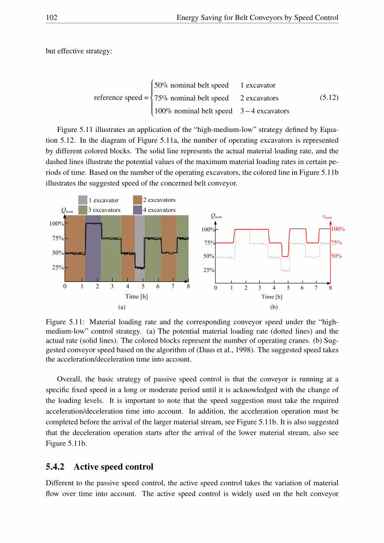
102 Energy Saving for Belt Conveyors by Speed Control
but effective strategy:
reference speed =
50% nominal belt speed 1 excavator
75% nominal belt speed 2 excavators
100% nominal belt speed 3−4 excavators
(5.12)
Figure 5.11 illustrates an application of the “high-medium-low” strategy defined by Equa-tion 5.12. In the diagram of Figure 5.11a, the number of operating excavators is representedby different colored blocks. The solid line represents the actual material loading rate, and thedashed lines illustrate the potential values of the maximum material loading rates in certain pe-riods of time. Based on the number of the operating excavators, the colored line in Figure 5.11billustrates the suggested speed of the concerned belt conveyor.
Qnom
1 2 3 4 5 6 7 8Time [h]
0
1 excavator 2 excavators4 excavators3 excavators
100%
75%
50%
25%
(a)
Qnom
1 2 3 4 5 6 7 8
vnom
0Time [h]
100%
75%
50%
100%
75%
50%
25%
(b)
Figure 5.11: Material loading rate and the corresponding conveyor speed under the “high-medium-low” control strategy. (a) The potential material loading rate (dotted lines) and theactual rate (solid lines). The colored blocks represent the number of operating cranes. (b) Sug-gested conveyor speed based on the algorithm of (Daus et al., 1998). The suggested speed takesthe acceleration/deceleration time into account.
Overall, the basic strategy of passive speed control is that the conveyor is running at aspecific fixed speed in a long or moderate period until it is acknowledged with the change ofthe loading levels. It is important to note that the speed suggestion must take the requiredacceleration/deceleration time into account. In addition, the acceleration operation must becompleted before the arrival of the larger material stream, see Figure 5.11b. It is also suggestedthat the deceleration operation starts after the arrival of the lower material stream, also seeFigure 5.11b.
5.4.2 Active speed control
Different to the passive speed control, the active speed control takes the variation of materialflow over time into account. The active speed control is widely used on the belt conveyor

Modeling of speed control systems 103
systems composed of multiple conveyors. In such cases, the material flow on the upstream beltconveyor is detected in real time, and the speed of the downstream conveyor(s) is adjusted tomatch the actual upcoming material flow.
Active speed control can be performed either in a continuous or discrete way. If the materialfeeding rate is varying slightly over time, active speed control can continuously adjust the beltspeed without high belt tension and without material spillage. If the variation is considerablylarge, like Scenario 3 in Section 5.1, the discrete control is suggested so that the belt speed canbe adjusted in a soft way.
5.4.2.1 Continuous control
The material flow sensor generally is installed at the upstream conveyor. It is assumed thatthe material requires time tdealy to travel from the installing location of the sensor to the load-ing area of the downstream conveyor. Then the instantaneous material feeding rate Qin of thedownstream conveyor can be approximated by
Qin(t) =Qdetect(t − tdealy) (5.13)
where Qdetect(t − tdealy) represents the material flow detected by the flow sensor at time point(t − tdealy). Accordingly, the theoretical instantaneous belt speed vth(t) can be calculated by
vth(t) =Qin(t)vnom
Qnom=
Qdetect(t − tdealy)Qnom
vnom (5.14)
If the theoretical belt speed can be strictly followed, then the cross section of the bulk materialonto the downstream belt conveyor is kept constant at the design value. Such control is thecontinuous active speed control.
Lodewijks et al. (2011) provide a case study of the continuous speed control. In the casestudy, the material flow is smoothly fluctuating in a sine wave with the cycle time 15 min-utes. The belt speed fluctuates to accommodate the fluctuating material feed in a strict manner.Simulation-based experimental results of (Lodewijks et al., 2011) show that the continuousspeed control can achieve considerable power savings in the studied condition.
However, matching the actual material flow in a strict way is not thus applicable in practice,since the actual material flow in most practical cases changes frequently to some extent. AsChapter 3 suggests, the fast and frequent transient operations can cause, for instance, the riskof belt over-tension and the risk of motor over-heating. Therefore, the continuous active speedcontrol generally is not recommended in practical operations.
5.4.2.2 Discrete control
For practical reasons, discrete speed control for belt conveyors is preferred above continuouscontrol, especially in the cases of the material flow with frequent and large variations. Pangand Lodewijks (2011) suggest that by means of discrete control, the belt speed can be adjustedin a soft way, and that the continuous acceleration operations with high belt tension can be
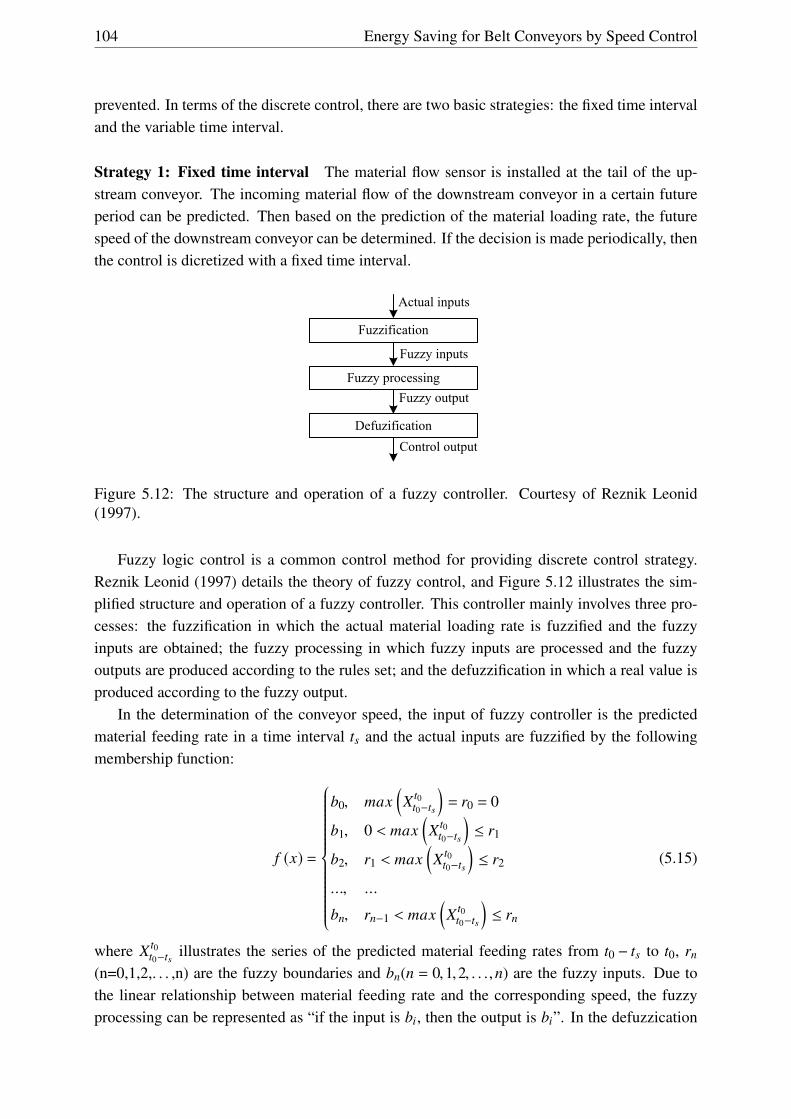
104 Energy Saving for Belt Conveyors by Speed Control
prevented. In terms of the discrete control, there are two basic strategies: the fixed time intervaland the variable time interval.
Strategy 1: Fixed time interval The material flow sensor is installed at the tail of the up-stream conveyor. The incoming material flow of the downstream conveyor in a certain futureperiod can be predicted. Then based on the prediction of the material loading rate, the futurespeed of the downstream conveyor can be determined. If the decision is made periodically, thenthe control is dicretized with a fixed time interval.
Fuzzification
Fuzzy processing
Defuzification
Actual inputs
Fuzzy inputs
Fuzzy output
Control output
Figure 5.12: The structure and operation of a fuzzy controller. Courtesy of Reznik Leonid(1997).
Fuzzy logic control is a common control method for providing discrete control strategy.Reznik Leonid (1997) details the theory of fuzzy control, and Figure 5.12 illustrates the sim-plified structure and operation of a fuzzy controller. This controller mainly involves three pro-cesses: the fuzzification in which the actual material loading rate is fuzzified and the fuzzyinputs are obtained; the fuzzy processing in which fuzzy inputs are processed and the fuzzyoutputs are produced according to the rules set; and the defuzzification in which a real value isproduced according to the fuzzy output.
In the determination of the conveyor speed, the input of fuzzy controller is the predictedmaterial feeding rate in a time interval ts and the actual inputs are fuzzified by the followingmembership function:
f (x) =
b0, max(X t0
t0−ts
)= r0 = 0
b1, 0 < max(X t0
t0−ts
)≤ r1
b2, r1 < max(X t0
t0−ts
)≤ r2
..., ...
bn, rn−1 < max(X t0
t0−ts
)≤ rn
(5.15)
where X t0t0−ts illustrates the series of the predicted material feeding rates from t0 − ts to t0, rn
(n=0,1,2,. . . ,n) are the fuzzy boundaries and bn(n = 0,1,2, . . .,n) are the fuzzy inputs. Due tothe linear relationship between material feeding rate and the corresponding speed, the fuzzyprocessing can be represented as “if the input is bi, then the output is bi”. In the defuzzication
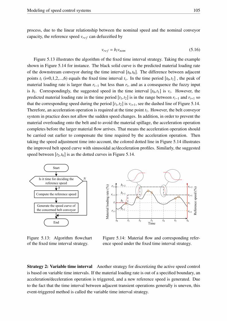
Modeling of speed control systems 105
process, due to the linear relationship between the nominal speed and the nominal conveyorcapacity, the reference speed vre f can defuzzified by
vre f = bivnom (5.16)
Figure 5.13 illustrates the algorithm of the fixed time interval strategy. Taking the exampleshown in Figure 5.14 for instance. The black solid curve is the predicted material loading rateof the downstream conveyor during the time interval [t0, t6]. The difference between adjacentpoints ti (i=0,1,2,...,6) equals the fixed time interval ts. In the time period [t0, t1] , the peak ofmaterial loading rate is larger than ri−1 but less than ri, and as a consequence the fuzzy inputis bi. Correspondingly, the suggested speed in the time interval [t0, t1] is vi. However, thepredicted material loading rate in the time period [t1, t2] is in the range between ri−1 and ri+1 sothat the corresponding speed during the period [t1, t2] is vi+1, see the dashed line of Figure 5.14.Therefore, an acceleration operation is required at the time point t1. However, the belt conveyorsystem in practice does not allow the sudden speed changes. In addition, in order to prevent thematerial overloading onto the belt and to avoid the material spillage, the acceleration operationcompletes before the larger material flow arrives. That means the acceleration operation shouldbe carried out earlier to compensate the time required by the acceleration operation. Thentaking the speed adjustment time into account, the colored dotted line in Figure 5.14 illustratesthe improved belt speed curve with sinusoidal ac/deceleration profiles. Similarly, the suggestedspeed between [t2, t6] is as the dotted curves in Figure 5.14.
Start
Is it time for deciding the reference speed
Compute the reference speed
Generate the speed curve of the concerned belt conveyor
End
Y
N
Figure 5.13: Algorithm flowchartof the fixed time interval strategy.
Mat
eria
l loa
ding
rate
(%)
Time
Ref
eren
ce sp
eed
(%)
ri
ri+1
ri+2
ri-1
vi
vi+1
vi+2
vi-1
t6t5t4t3t2t1t0
bi+2
bi+1
bi
bi-1
Figure 5.14: Material flow and corresponding refer-ence speed under the fixed time interval strategy.
Strategy 2: Variable time interval Another strategy for discretizing the active speed controlis based on variable time intervals. If the material loading rate is out of a specified boundary, anacceleration/deceleration operation is triggered, and a new reference speed is generated. Dueto the fact that the time interval between adjacent transient operations generally is uneven, thisevent-triggered method is called the variable time interval strategy.

106 Energy Saving for Belt Conveyors by Speed Control
Start
Compute the reference speed
Does the concerned belt conveyor require to adjust speed?
YGenerate the speed curve of the concerned belt conveyor
End
N
Figure 5.15: Algorithm flowchartof the variable time interval strat-egy.
Mat
eria
l loa
ding
rate
(%)
Time
Ref
eren
ce sp
eed
(%)
ri
ri+1
ri+2
ri-1
vi
vi+1
vi+2
vi-1
t0 t1 t2 t3 t4 t5 t6
bi+2
bi+1
bi
bi-1
Figure 5.16: Material flow and corresponding refer-ence speed under the variable time interval strategy.
Figure 5.15 represents the flowchart of algorithm of the variable time interval strategy. Dif-ferent to the algorithm of the fixed time interval strategy, this algorithm requires to compute thereference speed in each computational cycle. Figure 5.16 shows an application of the variabletime interval strategy, in which the profile of the predicted material loading rate onto the down-stream conveyor equals to that in Figure 5.14. In Figure 5.16, several certain threshold valuesfor feeding rate are defined. As the diagram shows, the material loading rate is in the range(ri−1,ri] in the time period [t0, t1). During this period, the conveyor is running at speed vi. Atthe time point t1, the material loading rate jumps out of the interval (ri−1,ri] and enters into theinterval (ri,ri+1]. Then a new reference speed vi+1 is generated, and an acceleration activity istriggered. Similarly, the acceleration or deceleration activities are triggered at time points t2, t3,t4, t5 and t6 in Figure 5.16. Correspondingly, the black dashed lines in Figure 5.16 illustratesthe suggested speed under the variable time interval strategy. Then taking the speed adjust-ment time into account, the colored dotted line shows the improved belt speed with sinusoidalac/deceleration profiles.
Conflicts and solutions To prevent being overloaded, the concerned belt conveyor shouldcomplete the acceleration operation before the arrival of the larger quantity material flow andit is suggested to start the deceleration after the arrival of the smaller quantity material flow.However, if the material feeding rate is varying frequently, there may exist a conflict betweenneighboring transient operations. Conflicts occur both in the fixed time interval strategy andthe variable time interval strategy. Taking the conditions in Figure 5.17 for instance wherethe variable time interval strategy is used. The diagram of Figure 5.17a illustrates the conflictbetween neighbored deceleration and acceleration operations. At the time point t1, the materialfeeding rate drops under ri−1. Based on the control strategy, the conveyor starts to lower speedfrom vi to vi−1 with the deceleration time tde. At the time point t2, the material feeding rateexceeds ri. To avoid the material spillage, the conveyor should start the acceleration from thetime point (t2− tac). If the sum of time tde and time tac is larger than the time interval (t2− t1),

Modeling of speed control systems 107
Time
Mat
eria
l loa
ding
rate
(%)
Ref
eren
ce sp
eed
(%)
ri
ri-1vi-1
vi
t1 t2
tde
tac
t1+tdet2-tac
(a)
Timet1 t2
tac
tac
t’ac
t2 -t’ac t1 -tac t2 -tac
Mat
eria
l loa
ding
rate
(%)
Ref
eren
ce sp
eed
(%)
ri
ri+1
ri-1
vi+1
vi-1
vi
(b)
Time
Mat
eria
l loa
ding
rate
(%)
Ref
eren
ce sp
eed
(%)
ri
ri+1
ri-1
vi+1
vi-1
vi
t1 t2
tdec
t’dec
tdec
t1 +tdec
t2 +tdec t1 +t’dec
(c)
Figure 5.17: Conflicts in discrete speed control. (a) Overlap between neighboring decelera-tion and acceleration operations. (b) Overlap between neighboring acceleration operations. (c)Overlap between neighboring deceleration operations.

108 Energy Saving for Belt Conveyors by Speed Control
then the conflict occurs as the black dotted lines illustrate in Figure 5.17a. In such cases, both thedeceleration and acceleration operations should be canceled, and a new speed curve is suggestedwhich is colored and dotted in Figure 5.17a.
The conflict also occurs in the cases where the material flow has a sudden and large variation.Taking the condition shown in Figure 5.17b for instance. At the time point t1, the materialloading rate exceeds ri−1. As planned, the conveyor should speed up from vi−1 to vi. It isassumed that this acceleration operation has no time conflicts with former transient operations,and then the acceleration operation can be performed in the time interval [t1− tac,t1]. At the timepoint t2, the material loading rate increases to above ri+1 so that another acceleration operation isexpected to be carried out to increase the conveyor speed to vi+1. Taking the conveyor dynamicsinto account, the second acceleration operation should start from the time point t2 − tac. If thetime point t2 − tac is prior to the time point t1, then the second acceleration overlaps with thefirst acceleration, see Figure 5.17b. In such cases, the two acceleration operations should becombined into one which is represented by the colored dotted line in Figure 5.17b. Similarly,the overlap between neighboring deceleration operations also can result in conflicts, as shownin Figure 5.17c. The solution is also given by the colored dotted line in Figure 5.17c.
Finally, taking the potential conflicts into account, Figure 5.18 gives the improved algorithmflowcharts of the discrete active speed control strategies.
Start
Is it time for deciding the reference speed
Does the new transient operation have conflicts with the former
transient operation?
Compute the reference speed
Solve the conflicts and reset the (former) reference speed
Does the concerned belt conveyor require to adjust speed?
Generate the speed curve of the concerned belt conveyor
End
Y
N
Y
N
Y
N
(a)
Start
Generate the reference speed
Does the new transient operation have conflicts with former
transient operation?
Does the concerned belt conveyor require to adjust speed?
Solve the conflicts and reset the (former) reference speed
Y
Y
Generate the speed curve of the concerned belt conveyor
End
N
N
(b)
Figure 5.18: Improved algorithm flowcharts of the discrete active speed control strategy. (a)Fixed time interval strategy. (b) Variable time interval strategy.

Modeling of speed control systems 109
5.4.3 Verification
Verification of the control system model is realized by using the dynamic simulations. Due tothe fact that the the passive speed control algorithm is very sample as compared to the activespeed control algorithm, herein we only discuss the verification of the active speed control sys-tem. The black curves in Figure 5.19 illustrates the predicted material loading rate onto theconcerned belt conveyor over 60 minutes. It is assumed that the reference speed set is definedas {40%,50%,60%,70%,80%,90%,100%} of nominal speed. It is further assumed that the per-mitted maximum acceleration is 0.1 m/s2 and that in terms of the fixed time interval strategy,the time interval is 30 seconds. The colored lines of Figure 5.19a illustrates the suggestedspeed under the fixed time interval strategy taking the acceleration/deceleration operations intoaccount. The colored lines of Figure 5.19b shows the simulation results of the variable time in-terval strategy. As these two diagrams show, the suggested speed curves are generated as plans,and the conflicts discussed above are successfully solved.
0 10 20 30 40 50 60Time [ min ]
0
20
40
60
80
100Loading rate (% of nominal capacity) Speed (% of nominal speed)
(a)
0 10 20 30 40 50 60Time [ min ]
0
20
40
60
80
100Loading rate (% of nominal capacity) Speed (% of nominal speed)
(b)
Figure 5.19: Verification of the model of the control system. (a) Fixed time interval strategy.(b) Variable time interval strategy.

110 Energy Saving for Belt Conveyors by Speed Control
5.5 Performances-Key Performance Indicators
The last section introduced several control strategies to build the simulation model of belt con-veyor speed control systems. This section defines several key performance indicators (KPIs) toevaluate the performance of speed control. Based on the importance of the indicators, the KPIsare classified into two groups: primary indicators and secondary indicators.
5.5.1 Primary KPIs
In terms of belt conveyor speed control, the primary KPIs majorly consist of the belt utilizationrate U, the power consumption P and the power saving ∆P. These indicators are the basicindicators which can be directly used for evaluating the performance of belt conveyors underdifferent control strategies. In the following of this section, these primary indicators will dis-cussed in detail.
Belt utilization rate U Belt utilization rate U is a percental difference between the actual andthe nominal cross sections of material on the belt. In the evaluation of speed control, the beltutilization rate is an important indicator. On the one hand, the actual value of the utilization ratesuggests the power saving potential by means of speed control. On the other hand, the differenceof the utilization rates between the nominal operation and the variable speed operation impliesthe performance of speed control. Taking the non-uniform distribution of material into account,the utilization rate can be calculated by
U =Average cross section of material on the beltNominal cross section of material on the belt
×100% (5.17)
Due to the linear relationship between the mass and the cross section of material, the utilizationrate can also be computed by
U =Total mass of material distributed on the belt
Nominal total material mass on the belt×100% (5.18)
Power consumption P and power saving ∆P Power consumption P in kW is another impor-tant indicator for evaluating speed control. The power consumption has two terms: one is themechanical power consumption Pm and another is the electric power consumption Pe. In thisand following chapters, the power consumption P refers to the electric power consumption Pe
if there is no special notation. The calculation method of the power consumption can be foundin Chapter 4. If it is assumed that in the nominal speed operation, the power consumption isPcon while Pnon represents for conditions with non-nominal speed, then the power saving ∆Pby means of speed control can be calculated by
∆P = Pcon−Pnon (5.19)
If the saving is represented by a percentage, then the calculation of the power saving can beexpressed by

Modeling of speed control systems 111
∆P =(1− Pnon
Pcon
)×100% (5.20)
5.5.2 Secondary KPIs
Secondary KPIs are the additional indicators of evaluating the performance of speed control.The values of these indicators are originated from the power consumption P. The secondaryKPIs mainly include the total energy consumption W , the electricity cost Costele, the carbondioxide (CO2) emissions EmissionCO2, the social cost of carbon SCC and the total cost Costtot .
Total power consumption W and energy saving ∆W Total power consumption W in kWh isthe amount of work done by belt conveyors and can be calculated by accumulating the instan-taneous power consumption over time
W =
´P (t)d (t)3600
=
∑P (t) tsample
3600(5.21)
where tsample is the sampling cycle time in s of the instantaneous power. Energy saving ∆W isthe difference of the energy consumption between the nominal speed operation and the variablespeed operation:
∆W =Wcon−Wnon (5.22)
where the subscribes con and non represent the operations with the constant-and-nominal speedand with the non-nominal-and variable speed, respectively.
Electricity cost Costele Electricity cost is the payment for consuming electricity during thematerial transportation, which takes the price of electricity into account. The price of electricityvaries widely from country to country and also may vary from time to time. Herein, the priceof electricity in the Netherlands is used to evaluate the electricity cost and it is assumed thatthe price is constant over time. According to the latest data from Eurostat (Eurostat, 2016),the price of electricity in the Netherlands averaged 0.1037eper kWh for industrial consumersduring the first half of 2016.
Carbon dioxide (CO2) emissions EmissionCO2 and their social cost SCC Air pollution, aby-product of electricity, can be extra considered in the evaluation of speed control. Carbondioxide (CO2), as a major source of greenhouse gases, is often used to describe the negativeimpacts of the electricity consumption. As United States Environmental Protection Agency(2015) suggested, the CO2 emissions also cause changes in net productivity, human health,property damages from increased flood risk, and changes in energy system costs. The value ofcarbon dioxide emission is variable over different activities, and the concept of emission factorEFCO2is widely used to calculate the total carbon emissions:
EmissionCO2 = EFCO2W (5.23)
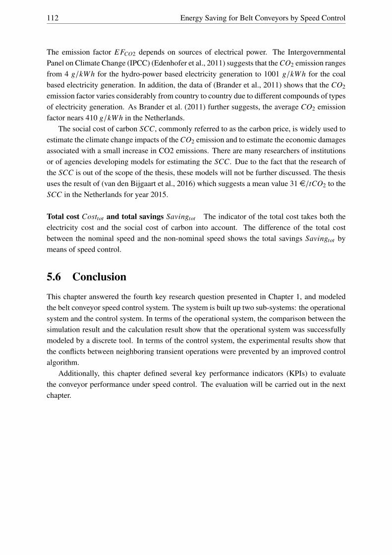
112 Energy Saving for Belt Conveyors by Speed Control
The emission factor EFCO2 depends on sources of electrical power. The IntergovernmentalPanel on Climate Change (IPCC) (Edenhofer et al., 2011) suggests that the CO2 emission rangesfrom 4 g/kWh for the hydro-power based electricity generation to 1001 g/kWh for the coalbased electricity generation. In addition, the data of (Brander et al., 2011) shows that the CO2
emission factor varies considerably from country to country due to different compounds of typesof electricity generation. As Brander et al. (2011) further suggests, the average CO2 emissionfactor nears 410 g/kWh in the Netherlands.
The social cost of carbon SCC, commonly referred to as the carbon price, is widely used toestimate the climate change impacts of the CO2 emission and to estimate the economic damagesassociated with a small increase in CO2 emissions. There are many researchers of institutionsor of agencies developing models for estimating the SCC. Due to the fact that the research ofthe SCC is out of the scope of the thesis, these models will not be further discussed. The thesisuses the result of (van den Bijgaart et al., 2016) which suggests a mean value 31 e/tCO2 to theSCC in the Netherlands for year 2015.
Total cost Costtot and total savings Savingtot The indicator of the total cost takes both theelectricity cost and the social cost of carbon into account. The difference of the total costbetween the nominal speed and the non-nominal speed shows the total savings Savingtot bymeans of speed control.
5.6 Conclusion
This chapter answered the fourth key research question presented in Chapter 1, and modeledthe belt conveyor speed control system. The system is built up two sub-systems: the operationalsystem and the control system. In terms of the operational system, the comparison between thesimulation result and the calculation result show that the operational system was successfullymodeled by a discrete tool. In terms of the control system, the experimental results show thatthe conflicts between neighboring transient operations were prevented by an improved controlalgorithm.
Additionally, this chapter defined several key performance indicators (KPIs) to evaluatethe conveyor performance under speed control. The evaluation will be carried out in the nextchapter.

Chapter 6
Simulation experimental results
Chapter 5 presented the modeling of the belt conveyor speed control system, in which the con-veyor system was viewed as a first-in-first-out buffer and a discrete tool was used to representthe continuous transport system. A series of computational simulations will be carried out inthis chapter to assess the performance of both the passive speed control and the active speedcontrol. In the assessment, the variable DIN f factor values will be used to calculate the powerconsumption of a belt conveyor. In addition, the acceleration and deceleration time also will betaken into account to ensure healthy dynamics of belt conveyors under speed control.
6.1 Introduction
Chapter 5 classified the bulk material loading scenarios into four groups and introduced severaldifferent types of belt conveyor speed control systems. In Scenario 1, the loading rate keepsconstant for a long term operation. If the loading rate is non-nominal, the passive speed controlis suggested and the conveyor is running at a fixed non-nominal speed. The passive speedcontrol also can be applied in Scenario 2 where the loading degree moderately varies in betweenlong term operations. In such cases, the conveyor speed is fixed until there is a considerablechange of the loading rate. If the loading degree is varying moderately in between short termoperations, see Scenarios 3 of Section 5.1, the passive speed control is not applicable any more.In such cases, the active speed control is highly suggested. Under the active speed control,the conveyor speed is frequently adjusted, as compared to the passive speed control, to matchthe actual loading rate. So that the concerned belt conveyor is expected to be running witha high utilization rate. However, if the actual loading varies excessively in all operations asin Scenario 4, the belt conveyor speed control is not suggested since the excessively frequentspeed adjustment can result in unhealthy conveyor dynamics.
The objective of this chapter is to study the performance of the speed control. Section 6.2will study a fictive belt conveyor system of an import bulk terminal to show performance ofthe passive speed control. Firstly, the assessment of the steady state performance of the passivespeed control will be carried out. In the steady state operation, the loading rate is constantand the conveyor is running at a fixed speed. Three kinds of bulk material will be used in theassessment. In addition, the variable value of the f factor defined by DIN 22101 (German
113

114 Energy Saving for Belt Conveyors by Speed Control
Institute for Standardization, 2015) will be taken into account to improve the accuracy of theassessment. Besides the static analysis, the dynamic performance of the passive speed controlalso will be studied where the loading rate is varying in between long term operations. Section6.3 studies another fictive belt conveyor system for assessing the active speed control. In theassessment, both the fixed time interval strategy and the variable time interval strategy will bestudied. In addition, in terms of the fixed time interval strategy, the influence of the speed setand of the time interval will be studied. Finally, conclusions are presented in Section 6.4.
6.2 Passive speed control
6.2.1 Setup
A fictive long horizontal belt conveyor in a fictive import dry bulk terminal is studied in thissection. The terminal is yearly operating for 360 days at 24 hours per day. Figure 6.1 shows thesimplified layout of the terminal and BC1-BC2-BC3 is one of the belt conveyor transport chains.The primary function of this terminal is as follows. The material in ships can be unloaded byfour cranes in parallel and discharged onto the BC1 belt. Then the material flow on the BC1 beltis in turn deposited onto the BC2 and BC3 belt conveyors, successively. Finally, the material isdischarged from the BC3 belt and stored at a stockyard by stackers.
Crane Belt conveyor
Transfer point
Seaside
LandsideBC1
BC
2
BC3
Stacker-Reclainmer
Figure 6.1: The layout of a fictive import terminal in which the BC2 belt conveyor is the studiedbelt conveyor.
The import terminal handles several types of dry bulk materials, including coal, limestoneand iron ore. Table 6.1 illustrates the parameters of these three kinds of bulk materials. Nomi-nally, the conveying capacity of the conveyor system is 2,000 MTPH, 3,500 MTPH and 6,000MTPH, in terms of coal, limestone and iron ore, respectively. However, with respect to thecrane-scheduling problem in practice, the number of operating cranes is variable-in-time dur-ing ship unloading. As a consequence, the material flow on the BC1-BC2-BC3 chain can beconsiderably lower than the design capacity. Based on the number of simultaneously operating

Simulation experimental results 115
cranes in a time interval, the ship unloading capacity during this time period however can be de-termined and the peak of the material feeding rate onto the belt conveyors can be approximated.Accordingly, the conveyor speed can be reduced to match the number of operating cranes andthen the utilization of belt conveyors is improved.
Table 6.1: Three sets of bulk material parameters. Courtesy of Spaans (1991).
Bulk material type Coal Limestone Iron oreDensity (kg/m3) 740 1,580 2,765Angle of internal friction (°) 32 45 35Frictional angle between belt and material (°) 15 15 15Angle of repose (°) 15 15 15
Table 6.2: Basic parameters of the BC2 conveyor.
Parameters Value Parameters ValueNominal conveying capacity (MTPH) 6,000 Belt type ST 1600Nominal speed (m/s) 5 Idler spacing (m) (top) 1.2Conveyor length in (m) 1000 (bottom) 3Conveyor height in (m) 0 Linear idlers weight (kg/m) 42.8Troughing angle (°) 30 Linear belt weight (kg/m) 39.4Special resistances (N) 0 Belt width (m) 1.2
As an example, the BC2 belt conveyor is studied, which has the largest useful conveyinglength in the BC1-BC2-BC3 chain. The studied belt conveyor is occupied for 40% of thetotal operation time of the terminal. Table 6.2 illustrates the parameters of the concerned beltconveyor. Taking the drive system efficiency into account, the permitted minimum conveyorspeed is defined as 2 m/s. Based on the linear relationship between the conveyor speed and theconveying capacity, the reference speed is classified into four levels:
Belt speed=
2 m/s 0−1 crane
2.5 m/s 2 cranes
3.8 m/s 3 cranes
5 m/s 4 cranes
(6.1)
6.2.2 Experiment plan
Several steady-state calculations and a dynamic simulation will be performed. Firstly, steady-state calculations are carried out to analyze the power savings, taking three kinds of bulk mate-rials into account. Table 6.1 lists the parameters of the bulk materials. In the static analyses, itis assumed that there always are 2 cranes operating simultaneously. Then it is further assumedthat the material loading rate is constant and equals half of the nominal conveying capacity. To

116 Energy Saving for Belt Conveyors by Speed Control
achieve various results and to compare the differences, calculation runs {1,3,5} in Table 6.3apply the nominal speed 5 m/s while runs {2,4,6} use a non-nominal speed, 2.5 m/s. Section6.2.3 details the steady-state calculations.
Table 6.3: Plan of Steady-state calculations.
Calculation run 1 2 3 4 5 6Bulk material Coal Limestone Iron oreLoading rate 1000 MTPH 1750 MTPH 3000 MTPH
Loading distribution Uniform Uniform Uniform Uniform Uniform UniformSpeed 5 m ⁄ s 2.5 m ⁄ s 5 m ⁄ s 2.5 m ⁄ s 5m ⁄ s 2.5 m ⁄ s
However, due to a possible problem of crane schedules, the number of operating cranesvaries over time. As a consequence, the material flow onto the concerned conveyor is variable-in-time. In addition, the actual material flow through the conveyor generally is non-uniform.To analyze the performance of passive speed control, a dynamic simulation is carried out. It isassumed that the number of operating cranes is varying from zero to four. The handling of coalis studied for instance and the actual material loading rate varies from zero to 2,000 MTPH.Section 6.2.4 discusses the dynamic simulation and illustrates the experimental results.
6.2.3 Steady-state calculation
Firstly, the variable values of the DIN f factor are achieved by the theoretical calculationmethod which was discussed in Chapter 4. Table 6.4 shows the calculation results of the ffactor over different loads and speeds. Taking the calculation run set {1,2} for instance wherethe bulk material conveyed is coal. The loading rate is half of the nominal conveying capacity.In Run 1, the conveyor is running at nominal speed and the conveyor belt is half loaded, whilein Run 2 the conveyor speed is lowered to ensure that the conveyor belt is fully loaded. Dueto the considerable increase of the bulk and belt flexural resistances, the f factor value showsa large increase when the conveyor is fully filled, see Table 6.4. As the data shows, the valueof the f factor in Run 2 is 0.0143 as compared to 0.0131 in Run 1. The considerable changeof the f factor value can also be found in the run set {3,4,5,6}. The operation in Runs 3 and 4conveys limestone and the operation of Runs 5 and 6 handles iron ore. Similar to Runs 1 and 2,the conveyors in these runs are loaded with half of the nominal conveying capacity. Runs 3 and5 uses the nominal speed and Runs 4 and 6 use a lower speed. As illustrated in Table 6.4, whenthe conveyor is running at a lower speed and the conveyor has a higher utilization, the DIN ffactor value has a considerable increase.
Taking the variable f factor values and different conveyor speeds into account, Table 6.5illustrates the power consumption of belt conveyors in different runs. All the static analysesshow positive results in the possibility to save power if the speed controlled operation is usedinstead of the nominal speed operation. Taking Runs 1 and 2 for instance. In Run 1, the powerconsumption is 137 kW . Due to the passive speed control, the power consumption in Run 2 isreduced by 36.8 kW , 27% of that in Run 1. This indicates that the passive speed control enables
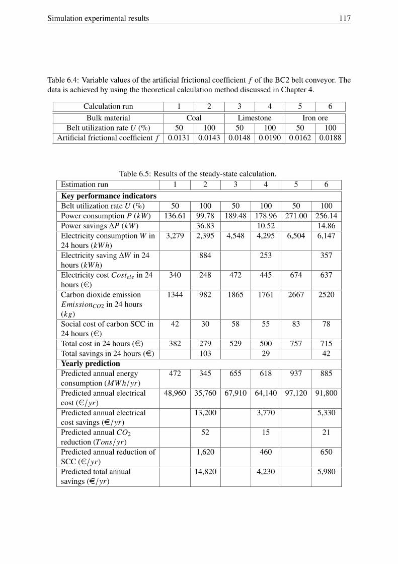
Simulation experimental results 117
Table 6.4: Variable values of the artificial frictional coefficient f of the BC2 belt conveyor. Thedata is achieved by using the theoretical calculation method discussed in Chapter 4.
Calculation run 1 2 3 4 5 6Bulk material Coal Limestone Iron ore
Belt utilization rate U (%) 50 100 50 100 50 100Artificial frictional coefficient f 0.0131 0.0143 0.0148 0.0190 0.0162 0.0188
Table 6.5: Results of the steady-state calculation.Estimation run 1 2 3 4 5 6Key performance indicatorsBelt utilization rate U (%) 50 100 50 100 50 100Power consumption P (kW) 136.61 99.78 189.48 178.96 271.00 256.14Power savings ∆P (kW) 36.83 10.52 14.86Electricity consumption W in24 hours (kWh)
3,279 2,395 4,548 4,295 6,504 6,147
Electricity saving ∆W in 24hours (kWh)
884 253 357
Electricity cost Costele in 24hours (e)
340 248 472 445 674 637
Carbon dioxide emissionEmissionCO2 in 24 hours(kg)
1344 982 1865 1761 2667 2520
Social cost of carbon SCC in24 hours (e)
42 30 58 55 83 78
Total cost in 24 hours (e) 382 279 529 500 757 715Total savings in 24 hours (e) 103 29 42Yearly predictionPredicted annual energyconsumption (MWh/yr)
472 345 655 618 937 885
Predicted annual electricalcost (e/yr)
48,960 35,760 67,910 64,140 97,120 91,800
Predicted annual electricalcost savings (e/yr)
13,200 3,770 5,330
Predicted annual CO2reduction (Tons/yr)
52 15 21
Predicted annual reduction ofSCC (e/yr)
1,620 460 650
Predicted total annualsavings (e/yr)
14,820 4,230 5,980

118 Energy Saving for Belt Conveyors by Speed Control
a considerable amount of power savings, although the f factor value in Run 2 is larger than thatin Run 1. The power saving can also be found in Runs 4 and 6 of Table 6.5.
Derived from the data of Table 6.5, Figure 6.2 illustrates and compares the power savingrates of the steady-state analyses. Taking the variation of the f factor into account, the savingsare between 5% and 27%. According to the data, the various saving rate highly depends onthe types of bulk materials. As the data in Figure 6.2 suggests, there is a negative correlationbetween the density of bulk materials and the saving rate. This suggestion can also be applied tothe cases where the f factor value is assumed to be fixed. The data in Figure 6.2 considers thecondition where the f factor is constant over loads and speeds. As the data shows, in terms ofcoal, the power saving can be up to 32% while in terms of iron ore, the saving ratio is reducedto 19%. In addition, the data of Figure 6.2 further suggests that compared to the conditionwith variable f factor values, the condition with a constant f factor over-estimates the powersavings, especially in the runs conveying limestone and iron ore. Therefore, it is important toconsider the variable values of the f factor to improve the accuracy of the assessment.
27%
6% 5%
32%
26%
19%
0%
5%
10%
15%
20%
25%
30%
35%
Coal (740kg/m3) Limestone (1580kg/m3) Iron ore(2765kg/m3)
Power saving rates
Variable f Constant f
Figure 6.2: Comparison of steady-state estimations.
The data of Table 6.5 also includes the value of other key performance indicators. Forexample, the results of yearly predictions are given. As the data shows, a large amount ofelectricity cost and carbon emission can be saved by speed control. Taking the transportation ofcoal for instance. Due to the passive speed control, the electricity cost yearly can be reduced bye13,200 with 52 tons of carbon emission. If the social cost of carbon is taken into account, thetotal annual savings can be up to e14,820.
Further calculation and discussion The data in Table 6.4 shows that the DIN f factor valuevaries with loads and speeds. It further shows that when the conveyor speed is reduced, the DINf factor increases considerably due to the increase of the load. Therefore, taking the variableDIN f values into account, it is important to find the optimum conveyor speed for maximumpower reduction before the application of speed control. Further steady-state calculations are

Simulation experimental results 119
Tabl
e6.
6:V
alue
sof
the
DIN
ffa
ctor
over
diff
eren
tlo
ads
and
spee
ds.
The
conv
eyor
islo
aded
byco
alw
ithde
nsity
740
kg/m
3 .T
helo
adis
repr
esen
ted
byth
eco
nvey
orut
iliza
tion
U,v
aryi
ngfr
om10
%to
100%
.The
conv
eyor
spee
dV
isin
the
rang
efr
om2
m/s
to5
m/s
.
VU
10%
20%
30%
40%
50%
60%
70%
80%
90%
100%
20.
0099
0.00
990.
0100
0.01
020.
0105
0.01
090.
0114
0.01
200.
0127
0.01
352.
250.
0102
0.01
020.
0104
0.01
060.
0109
0.01
130.
0118
0.01
240.
0131
0.01
392.
50.
0105
0.01
050.
0107
0.01
090.
0113
0.01
170.
0122
0.01
280.
0135
0.01
432.
750.
0107
0.01
080.
0110
0.01
120.
0116
0.01
200.
0125
0.01
310.
0138
0.01
463
0.01
100.
0110
0.01
120.
0115
0.01
180.
0123
0.01
280.
0134
0.01
410.
0149
3.25
0.01
110.
0112
0.01
140.
0117
0.01
210.
0125
0.01
310.
0137
0.01
440.
0152
3.5
0.01
130.
0114
0.01
160.
0119
0.01
230.
0127
0.01
330.
0139
0.01
460.
0154
3.75
0.01
140.
0116
0.01
180.
0121
0.01
250.
0129
0.01
350.
0141
0.01
480.
0156
40.
0115
0.01
170.
0119
0.01
220.
0126
0.01
310.
0137
0.01
430.
0150
0.01
584.
250.
0116
0.01
180.
0120
0.01
240.
0128
0.01
320.
0138
0.01
450.
0152
0.01
604.
50.
0117
0.01
190.
0121
0.01
250.
0129
0.01
340.
0139
0.01
460.
0153
0.01
614.
750.
0118
0.01
200.
0122
0.01
250.
0130
0.01
350.
0140
0.01
470.
0154
0.01
625
0.01
180.
0120
0.01
230.
0126
0.01
310.
0136
0.01
410.
0148
0.01
550.
0163

120 Energy Saving for Belt Conveyors by Speed Control
0
100
20
Pow
er c
onsu
mpt
ion
(kW
)
200
40
300
5
Loading rate(% of Qnom)
4.560 4
Speed (m/s)
3.580 32.5
100 2
(a)
Speed rate (%)40 60 80 100
Load
ing
rate
(%
)
20
40
60
80
100
0
10
20
30
40
50
60
(b)
Figure 6.3: Calculation results. The loading rate varies from 10% to 100% of the nominalconveying capacity. The conveyor speed varies from 2 m/s to 5 m/s. The speed ratio is noless than the loading ratio to avoid the material spilling from the belt. (a) Power consumptionfor different loading rates and for different speeds. (b) Power saving ratio for different loadingrates and for different speeds.
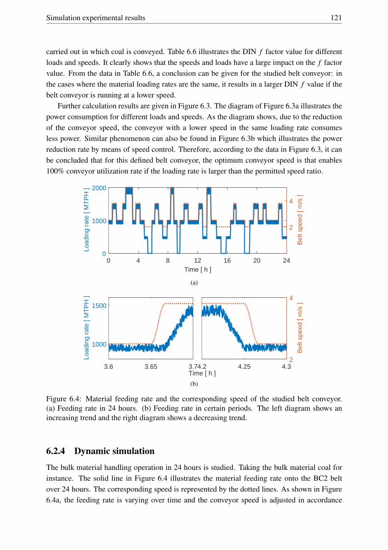
Simulation experimental results 121
carried out in which coal is conveyed. Table 6.6 illustrates the DIN f factor value for differentloads and speeds. It clearly shows that the speeds and loads have a large impact on the f factorvalue. From the data in Table 6.6, a conclusion can be given for the studied belt conveyor: inthe cases where the material loading rates are the same, it results in a larger DIN f value if thebelt conveyor is running at a lower speed.
Further calculation results are given in Figure 6.3. The diagram of Figure 6.3a illustrates thepower consumption for different loads and speeds. As the diagram shows, due to the reductionof the conveyor speed, the conveyor with a lower speed in the same loading rate consumesless power. Similar phenomenon can also be found in Figure 6.3b which illustrates the powerreduction rate by means of speed control. Therefore, according to the data in Figure 6.3, it canbe concluded that for this defined belt conveyor, the optimum conveyor speed is that enables100% conveyor utilization rate if the loading rate is larger than the permitted speed ratio.
0 4 8 12 16 20 24Time [ h ]
0
1000
2000
Load
ing
rate
[ M
TP
H ]
2
4
Bel
t spe
ed [
m/s
]
(a)
3.6 3.65 3.7
1000
1500
Load
ing
rate
[ M
TP
H ]
4.2 4.25 4.3Time [ h ]
2
4B
elt s
peed
[ m
/s ]
(b)
Figure 6.4: Material feeding rate and the corresponding speed of the studied belt conveyor.(a) Feeding rate in 24 hours. (b) Feeding rate in certain periods. The left diagram shows anincreasing trend and the right diagram shows a decreasing trend.
6.2.4 Dynamic simulation
The bulk material handling operation in 24 hours is studied. Taking the bulk material coal forinstance. The solid line in Figure 6.4 illustrates the material feeding rate onto the BC2 beltover 24 hours. The corresponding speed is represented by the dotted lines. As shown in Figure6.4a, the feeding rate is varying over time and the conveyor speed is adjusted in accordance
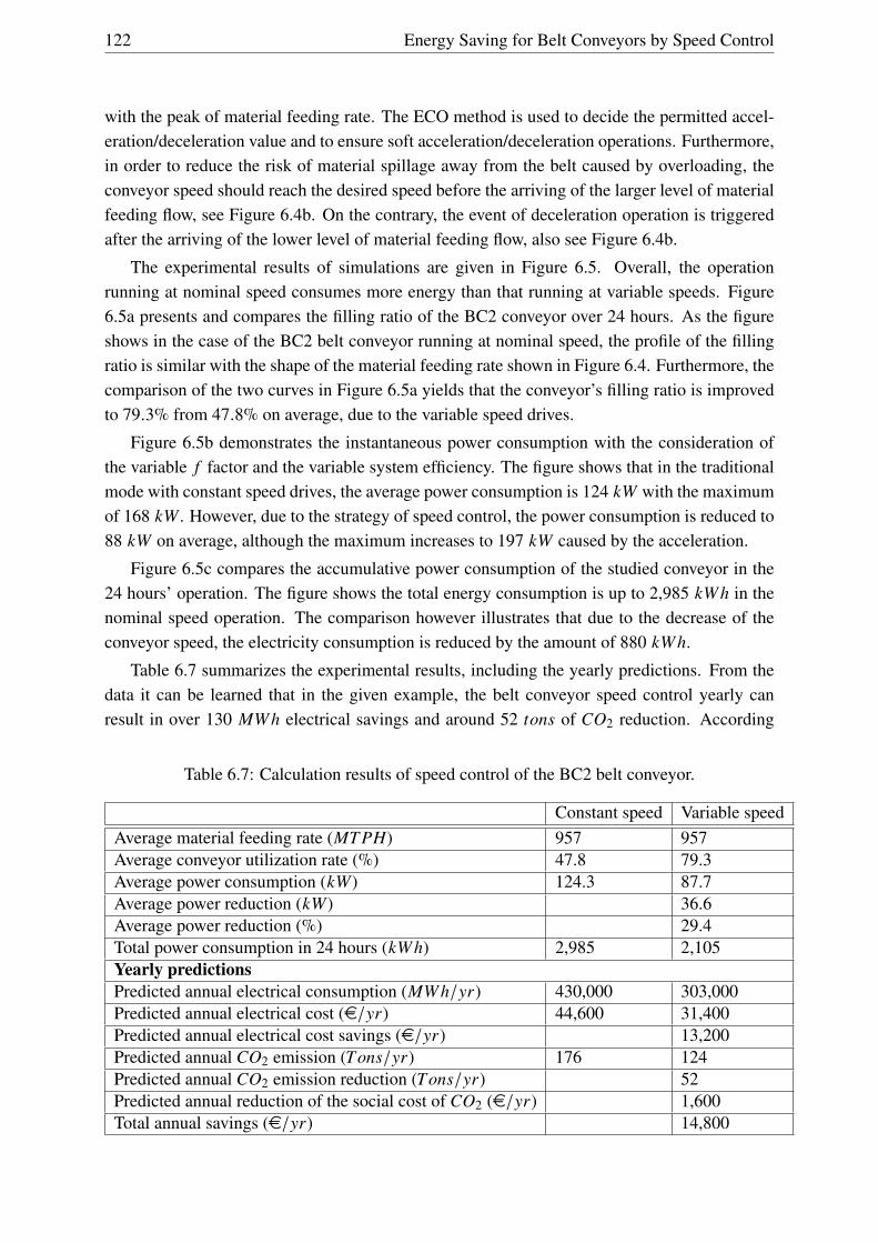
122 Energy Saving for Belt Conveyors by Speed Control
with the peak of material feeding rate. The ECO method is used to decide the permitted accel-eration/deceleration value and to ensure soft acceleration/deceleration operations. Furthermore,in order to reduce the risk of material spillage away from the belt caused by overloading, theconveyor speed should reach the desired speed before the arriving of the larger level of materialfeeding flow, see Figure 6.4b. On the contrary, the event of deceleration operation is triggeredafter the arriving of the lower level of material feeding flow, also see Figure 6.4b.
The experimental results of simulations are given in Figure 6.5. Overall, the operationrunning at nominal speed consumes more energy than that running at variable speeds. Figure6.5a presents and compares the filling ratio of the BC2 conveyor over 24 hours. As the figureshows in the case of the BC2 belt conveyor running at nominal speed, the profile of the fillingratio is similar with the shape of the material feeding rate shown in Figure 6.4. Furthermore, thecomparison of the two curves in Figure 6.5a yields that the conveyor’s filling ratio is improvedto 79.3% from 47.8% on average, due to the variable speed drives.
Figure 6.5b demonstrates the instantaneous power consumption with the consideration ofthe variable f factor and the variable system efficiency. The figure shows that in the traditionalmode with constant speed drives, the average power consumption is 124 kW with the maximumof 168 kW . However, due to the strategy of speed control, the power consumption is reduced to88 kW on average, although the maximum increases to 197 kW caused by the acceleration.
Figure 6.5c compares the accumulative power consumption of the studied conveyor in the24 hours’ operation. The figure shows the total energy consumption is up to 2,985 kWh in thenominal speed operation. The comparison however illustrates that due to the decrease of theconveyor speed, the electricity consumption is reduced by the amount of 880 kWh.
Table 6.7 summarizes the experimental results, including the yearly predictions. From thedata it can be learned that in the given example, the belt conveyor speed control yearly canresult in over 130 MWh electrical savings and around 52 tons of CO2 reduction. According
Table 6.7: Calculation results of speed control of the BC2 belt conveyor.
Constant speed Variable speedAverage material feeding rate (MTPH) 957 957Average conveyor utilization rate (%) 47.8 79.3Average power consumption (kW) 124.3 87.7Average power reduction (kW) 36.6Average power reduction (%) 29.4Total power consumption in 24 hours (kWh) 2,985 2,105Yearly predictionsPredicted annual electrical consumption (MWh/yr) 430,000 303,000Predicted annual electrical cost (e/yr) 44,600 31,400Predicted annual electrical cost savings (e/yr) 13,200Predicted annual CO2 emission (Tons/yr) 176 124Predicted annual CO2 emission reduction (Tons/yr) 52Predicted annual reduction of the social cost of CO2 (e/yr) 1,600Total annual savings (e/yr) 14,800
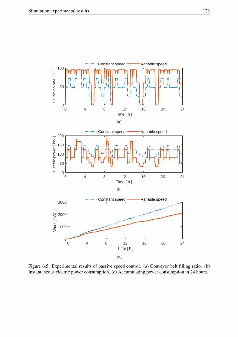
Simulation experimental results 123
Time [ h ]0 4 8 12 16 20 24
Util
izat
ion
rate
[ %
]
0
50
100Constant speed Variable speed
(a)
Time [ h ]0 4 8 12 16 20 24
Ele
ctric
pow
er [
kW ]
0
50
100
150
200Constant speed Variable speed
(b)
Time [ h ]0 4 8 12 16 20 24
Wor
k [ k
Wh
]
0
1000
2000
3000Constant speed Variable speed
(c)
Figure 6.5: Experimental results of passive speed control. (a) Conveyor belt filling ratio. (b)Instantaneous electric power consumption. (c) Accumulating power consumption in 24 hours.
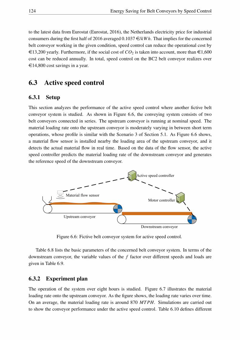
124 Energy Saving for Belt Conveyors by Speed Control
to the latest data from Eurostat (Eurostat, 2016), the Netherlands electricity price for industrialconsumers during the first half of 2016 averaged 0.1037e/kWh. That implies for the concernedbelt conveyor working in the given condition, speed control can reduce the operational cost bye13,200 yearly. Furthermore, if the social cost of CO2 is taken into account, more than e1,600cost can be reduced annually. In total, speed control on the BC2 belt conveyor realizes overe14,800 cost savings in a year.
6.3 Active speed control
6.3.1 Setup
This section analyzes the performance of the active speed control where another fictive beltconveyor system is studied. As shown in Figure 6.6, the conveying system consists of twobelt conveyors connected in series. The upstream conveyor is running at nominal speed. Thematerial loading rate onto the upstream conveyor is moderately varying in between short termoperations, whose profile is similar with the Scenario 3 of Section 5.1. As Figure 6.6 shows,a material flow sensor is installed nearby the loading area of the upstream conveyor, and itdetects the actual material flow in real time. Based on the data of the flow sensor, the activespeed controller predicts the material loading rate of the downstream conveyor and generatesthe reference speed of the downstream conveyor.
Material flow sensor
Downstream conveyor
Upstream conveyor
Active speed controller
Motor controller
Figure 6.6: Fictive belt conveyor system for active speed control.
Table 6.8 lists the basic parameters of the concerned belt conveyor system. In terms of thedownstream conveyor, the variable values of the f factor over different speeds and loads aregiven in Table 6.9.
6.3.2 Experiment plan
The operation of the system over eight hours is studied. Figure 6.7 illustrates the materialloading rate onto the upstream conveyor. As the figure shows, the loading rate varies over time.On an average, the material loading rate is around 870 MTPH. Simulations are carried outto show the conveyor performance under the active speed control. Table 6.10 defines different

Simulation experimental results 125
Table 6.8: Parameters of the belt conveyors.
Parameters Value Parameters ValueNominal conveying capacity (MTPH) 2,000 Belt type ST 800Nominal speed (m/s) 5 Ilder spacing (m) (top) 1.2Conveyor length (m) Upstream 300 (bottom) 3
Downstream 1000 Linear idlers weight (kg/m) 27.1Conveyor height (m) 0 Linear belt weight (kg/m) 23Troughing angle (°) 30 Belt width (m) 1.2Density of bulk material (Coal) (kg/m3) 740 Special resistances (N) 0
0 1 2 3 4 5 6 7 8Time [ h ]
0
500
1000
1500
2000
Mat
eria
l loa
ding
rat
e [ M
TP
H ]
Figure 6.7: Material loading rate onto the upstream conveyor.
simulation runs in order to produce various results. Run 1 is the operation running at nominalspeed, and the experimental result of Run 1 is the benchmark of the active speed control. Interms of the fixed time interval strategy, the run set {2,3,4,5} considers different speed setswhich are determined by the adjacent speed difference. In Run 2, for instance, the speed setis {2,2.25,2.5,...,4.5,4.75,5} in m/s and the adjacent speed difference is 0.25 m/s. The run set{3,6,7} studies the behaviors of the controller under different time intervals. The run set {3,8}compares the difference between the fixed time interval strategy and the variable time intervalstrategy.

126 Energy Saving for Belt Conveyors by Speed Control
Table6.9:
Values
ofthe
DIN
ffactor
overdifferent
loadsand
speeds.T
heconveyor
isloaded
bycoal
with
density740
kg/m
3.T
heload
isrepresented
bythe
conveyorutilization
U,varying
from0
to100%
.T
heconveyor
speedV
isin
therange
from2
m/s
to5
m/s
with
adiscrete
interval0.25m/s.T
heconveyoris
pre-tensionedw
ith30
kN.
VU
010%
20%30%
40%50%
60%70%
80%90%
100%
20.0122
0.01180.0116
0.01170.0119
0.01240.0129
0.01370.0146
0.01550.0166
2.250.0125
0.01200.0119
0.01200.0122
0.01270.0133
0.01400.0149
0.01590.0170
2.50.0127
0.01220.0121
0.01220.0125
0.01300.0136
0.01430.0152
0.01620.0173
2.750.0129
0.01240.0123
0.01250.0128
0.01320.0139
0.01460.0155
0.01650.0175
30.0130
0.01260.0125
0.01260.0130
0.01340.0141
0.01480.0157
0.01670.0178
3.250.0131
0.01270.0127
0.01280.0131
0.01360.0143
0.01500.0159
0.01690.0180
3.50.0132
0.01280.0128
0.01290.0133
0.01380.0144
0.01520.0161
0.01710.0182
3.750.0133
0.01290.0129
0.01300.0134
0.01390.0146
0.01530.0162
0.01720.0183
40.0134
0.01300.0130
0.01310.0135
0.01400.0147
0.01550.0164
0.01740.0184
4.250.0135
0.01310.0130
0.01320.0136
0.01410.0148
0.01550.0165
0.01750.0185
4.50.0135
0.01310.0131
0.01330.0136
0.01420.0148
0.01560.0165
0.01750.0186
4.750.0136
0.01320.0131
0.01330.0137
0.01420.0149
0.01570.0166
0.01760.0187
50.0136
0.01320.0132
0.01340.0137
0.01430.0149
0.01570.0166
0.01760.0187
Table6.10:E
xperimentplan
oftheactive
speedcontrol.
Simulation
run1
23
4C
ontrolstrategyN
ominalspeed
Fixedtim
einterval
Time
interval-
30seconds
Speedset(m
/s){5}
{2,2.25,2.5,...,4.5,4.75,5}{2,2.5,3...,4.5,5}
{2,3,4,5}
Simulation
run5
67
8C
ontrolstrategyFixed
time
intervalV
ariabletim
einterval
Time
interval30s
20seconds
10seconds
Variable
Speedset(m
/s){2,3.5,5}
{2,2.5,3...,4.5,5}

Simulation experimental results 127
6.3.3 Results and Discussion
Table 6.11 shows the experimental results of simulation runs. Due to the fact that the upstreamconveyor consistently is running at nominal speed in these eight simulation runs, the simula-tion results of the upstream conveyor are excluded. As the data in Table 6.11 shows, all thesimulation runs achieve power savings if the concerned belt conveyor is actively controlled.
Table 6.11: Experimental results of the downstream conveyor under active speed control over 8hours.
Simulation run 1 2 3 4 5 6 7 8
Total conveying in eight hours (tons) 6,900Average loading rate Q(MTPH) 866Average speed v(m/s) 5 3.02 3.09 3.23 3.39 3.04 2.99 2.95Average conveyor utilization U(%) 43.4 67.0 65.5 62.2 59.2 66.5 67.8 68.8Average power consumption P(kW) 97.4 70.0 70.8 72.5 75.3 70.2 69.6 68.9Power saving ∆P (kW) - 27.4 26.6 25.0 22.1 27.2 27.8 28.5
(%) - 28 27 26 23 28 29 29Electricity consumption W(kWh) 779 560 566 580 602 562 557 551Consumption saving∆W(kWh) - 219 213 200 177 218 223 228
Figure 6.8 shows the influence of speed sets under the fixed time interval strategy. In Run2, the minimum speed increment is 0.25 m/s and the speed set has 13 elements. However, inRuns 3 to 5, the minimum increment is defined as 0.5 m/s, 1 m/s and 1.5 m/s, respectively.Accordingly, the number of elements is reduced to 7, 4 and 3, respectively. Generally, thesmaller the minimum increment is, the more sensitive the speed controller is and the morepower you can save. This is proved by the comparison in Figure 6.8. The diagram of Figure6.8a illustrates the average conveyor utilization in each hour and Figure 6.8b shows the averagepower consumption. As the data shows, Run 2 consistently results in the highest utilizationrate. By way of contrast, the result of Run 5 shows the lowest average utilization rate. This isalso proved by the data in Table 6.11. Over the eight hours’ operation, the utilization in Run 2reaches up to 67% as compared to 29% in Run 5. Correspondingly, Run 2 uses the least numberof electricity and Run 5 consumes the most, see Table 6.11 and Figure 6.8b.
The simulation run sets {3,6,7} studies different time intervals of the fixed time intervalstrategy. In Run 3, the time interval is set to 30 seconds, while the value in Runs 6 and 7 is 20and 10 seconds, respectively. The experimental results are illustrated in Figure 6.9. The dataof Figure 6.9a shows that the high utilization rate can be achieved when a small time intervalis used. As a consequence, Runs 6 and 7 consume less power compared to Run 3, see Figure6.9b. In addition, the comparison between Figures 6.8 and 6.9 suggests that the definition ofthe speed set has a larger impact on the energy savings than the selection of the time interval.
Figure 6.10 compares the fixed and variable time interval strategies. Run 3 uses the fixedtime interval strategy and Run 8 employs the variable time interval strategy. The definitions ofthe speed set in Runs 3 and 8 are the same, {2,2.5,3,..,4,4.5,5} in m/s. The diagram of Figure6.10a compares the conveyor utilization over time. As the diagram indicates, the utilization
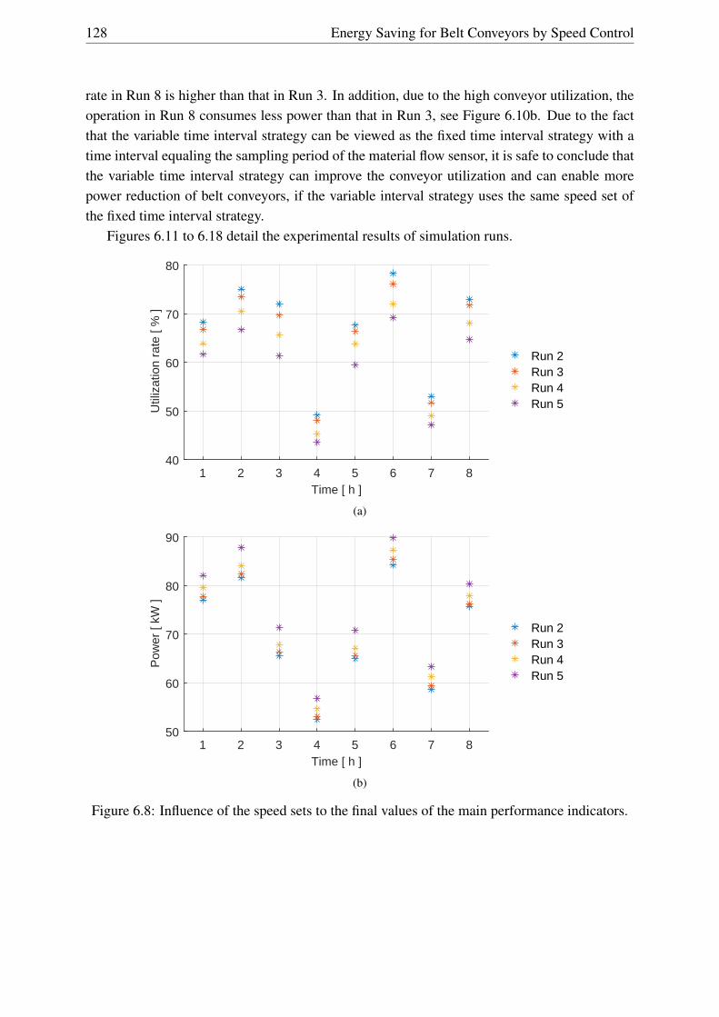
128 Energy Saving for Belt Conveyors by Speed Control
rate in Run 8 is higher than that in Run 3. In addition, due to the high conveyor utilization, theoperation in Run 8 consumes less power than that in Run 3, see Figure 6.10b. Due to the factthat the variable time interval strategy can be viewed as the fixed time interval strategy with atime interval equaling the sampling period of the material flow sensor, it is safe to conclude thatthe variable time interval strategy can improve the conveyor utilization and can enable morepower reduction of belt conveyors, if the variable interval strategy uses the same speed set ofthe fixed time interval strategy.
Figures 6.11 to 6.18 detail the experimental results of simulation runs.
1 2 3 4 5 6 7 8Time [ h ]
40
50
60
70
80
Util
izat
ion
rate
[ %
]
Run 2Run 3Run 4Run 5
(a)
1 2 3 4 5 6 7 8Time [ h ]
50
60
70
80
90
Pow
er [
kW ]
Run 2Run 3Run 4Run 5
(b)
Figure 6.8: Influence of the speed sets to the final values of the main performance indicators.
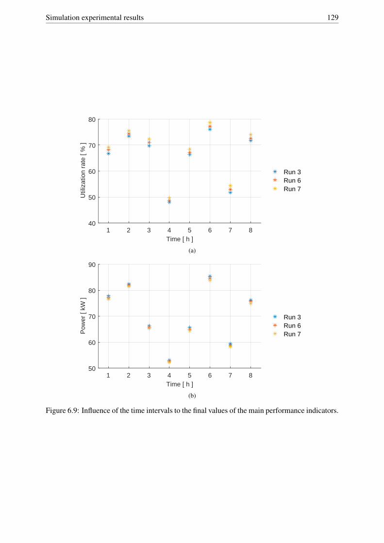
Simulation experimental results 129
1 2 3 4 5 6 7 8Time [ h ]
40
50
60
70
80
Util
izat
ion
rate
[ %
]
Run 3Run 6Run 7
(a)
1 2 3 4 5 6 7 8Time [ h ]
50
60
70
80
90
Pow
er [
kW ]
Run 3Run 6Run 7
(b)
Figure 6.9: Influence of the time intervals to the final values of the main performance indicators.

130 Energy Saving for Belt Conveyors by Speed Control
1 2 3 4 5 6 7 8Time [ h ]
40
50
60
70
80
Util
izat
ion
rate
[ %
]
Run 3Run 8
(a)
1 2 3 4 5 6 7 8Time [ h ]
50
60
70
80
90
Pow
er [
kW ]
Run 3Run 8
(b)
Figure 6.10: Influence of the control strategy to the final values of the main performance indi-cators.

Simulation experimental results 131
2
3
4
5
Spe
ed [
m/s
]
0
500
1000
1500
2000
Unl
oadi
ng r
ate
[ MT
PH
]
0
50
100
Util
izat
ion
[ % ]
0
50
100
150
200
Pow
er (
kW)
0 1 2 3 4 5 6 7 8Time [ h ]
0
300
600
900
Wor
k [ k
Wh
]
Figure 6.11: Experimental results of Run 1 where the conveyor is running at nominal speed.Averagely, the conveyor utilization is 43.4% and the power consumption is 97 kW . After eighthours’ operation, the total energy consumption is around 780 kWh.

132 Energy Saving for Belt Conveyors by Speed Control
2
3
4
5
Spe
ed [
m/s
]
0
500
1000
1500
2000
Unl
oadi
ng r
ate
[ MT
PH
]
0
50
100
Util
izat
ion
[ % ]
0
50
100
150
200
Pow
er (
kW)
0 1 2 3 4 5 6 7 8Time [ h ]
0
300
600
900
Wor
k [ k
Wh
]
Figure 6.12: Experimental results of Run 2 where the conveyor speed is actively controlledwith the fixed time interval strategy. The time interval is 30 seconds. The speed set is{2,2.25,2.5,..,4.5,4.75,5} in m/s. Averagely, the conveyor speed is 3.02 m/s and the conveyorutilization is 67.0%. The power consumption is 70 kW in an average. After eight hours’ opera-tion, the total energy consumption is 560 kWh.

Simulation experimental results 133
2
3
4
5
Spe
ed [
m/s
]
0
500
1000
1500
2000
Unl
oadi
ng r
ate
[ MT
PH
]
0
50
100
Util
izat
ion
[ % ]
0
50
100
150
200
Pow
er (
kW)
0 1 2 3 4 5 6 7 8Time [ h ]
0
300
600
900
Wor
k [ k
Wh
]
Figure 6.13: Experimental results of Run 3 where the conveyor speed is actively controlledwith the fixed time interval strategy. The time interval is 30 seconds. The speed set is{2,2.5,3,..,4,4.5,5} in m/s. Averagely, the conveyor speed is 3.09 m/s and the conveyor utiliza-tion is 65.5%. The power consumption is 71 kW in an average. After eight hours’ operation,the total energy consumption is 566 kWh.

134 Energy Saving for Belt Conveyors by Speed Control
2
3
4
5
Spe
ed [
m/s
]
0
500
1000
1500
2000
Unl
oadi
ng r
ate
[ MT
PH
]
0
50
100
Util
izat
ion
[ % ]
0
50
100
150
200
Pow
er (
kW)
0 1 2 3 4 5 6 7 8Time [ h ]
0
300
600
900
Wor
k [ k
Wh
]
Figure 6.14: Experimental results of Run 4 where the conveyor speed is actively controlled withthe fixed time interval strategy. The time interval is 30 seconds. The speed set is {2,3,4,5} inm/s. Averagely, the conveyor speed is 3.23 m/s and the conveyor utilization is 62.2%. Thepower consumption is 72.5 kW in an average. After eight hours’ operation, the total energyconsumption is 580 kWh.
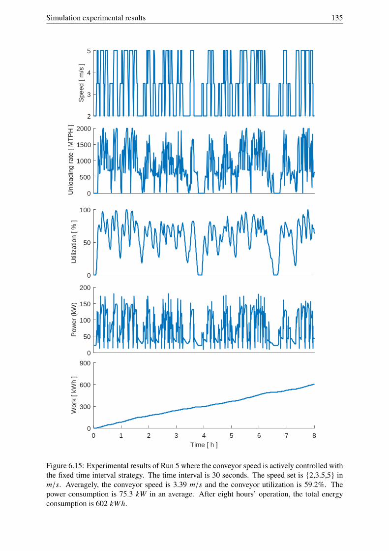
Simulation experimental results 135
2
3
4
5
Spe
ed [
m/s
]
0
500
1000
1500
2000
Unl
oadi
ng r
ate
[ MT
PH
]
0
50
100
Util
izat
ion
[ % ]
0
50
100
150
200
Pow
er (
kW)
0 1 2 3 4 5 6 7 8Time [ h ]
0
300
600
900
Wor
k [ k
Wh
]
Figure 6.15: Experimental results of Run 5 where the conveyor speed is actively controlled withthe fixed time interval strategy. The time interval is 30 seconds. The speed set is {2,3.5,5} inm/s. Averagely, the conveyor speed is 3.39 m/s and the conveyor utilization is 59.2%. Thepower consumption is 75.3 kW in an average. After eight hours’ operation, the total energyconsumption is 602 kWh.

136 Energy Saving for Belt Conveyors by Speed Control
2
3
4
5
Spe
ed [
m/s
]
0
500
1000
1500
2000
Unl
oadi
ng r
ate
[ MT
PH
]
0
50
100
Util
izat
ion
[ % ]
0
50
100
150
200
Pow
er (
kW)
0 1 2 3 4 5 6 7 8Time [ h ]
0
300
600
900
Wor
k [ k
Wh
]
Figure 6.16: Experimental results of Run 6 where the conveyor speed is actively controlledwith the fixed time interval strategy. The time interval is 20 seconds. The speed set is{2,2.5,3,..,4,4.5,5} in m/s. Averagely, the conveyor speed is 3.04 m/s and the conveyor utiliza-tion is 66.5%. The power consumption is 70.2 kW in an average. After eight hours’ operation,the total energy consumption is 562 kWh.

Simulation experimental results 137
2
3
4
5
Spe
ed [
m/s
]
0
500
1000
1500
2000
Unl
oadi
ng r
ate
[ MT
PH
]
0
50
100
Util
izat
ion
[ % ]
0
50
100
150
200
Pow
er (
kW)
0 1 2 3 4 5 6 7 8Time [ h ]
0
300
600
900
Wor
k [ k
Wh
]
Figure 6.17: Experimental results of Run 7 where the conveyor speed is actively controlledwith the fixed time interval strategy. The time interval is 10 seconds. The speed set is{2,2.5,3,..,4,4.5,5} in m/s. Averagely, the conveyor speed is 2.99 m/s and the conveyor utiliza-tion is 67.8%. The power consumption is 69.6 kW in an average. After eight hours’ operation,the total energy consumption is 557 kWh.
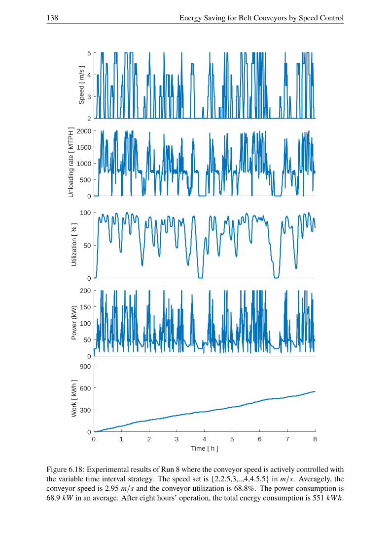
138 Energy Saving for Belt Conveyors by Speed Control
2
3
4
5
Spe
ed [
m/s
]
0
500
1000
1500
2000
Unl
oadi
ng r
ate
[ MT
PH
]
0
50
100
Util
izat
ion
[ % ]
0
50
100
150
200
Pow
er (
kW)
0 1 2 3 4 5 6 7 8Time [ h ]
0
300
600
900
Wor
k [ k
Wh
]
Figure 6.18: Experimental results of Run 8 where the conveyor speed is actively controlled withthe variable time interval strategy. The speed set is {2,2.5,3,..,4,4.5,5} in m/s. Averagely, theconveyor speed is 2.95 m/s and the conveyor utilization is 68.8%. The power consumption is68.9 kW in an average. After eight hours’ operation, the total energy consumption is 551 kWh.

Simulation experimental results 139
6.4 Conclusion
This chapter analyzed and compared the conveyor performance under difference control man-ners. Based on the experimental results, a general conclusion can be given that the powerconsumption can be reduced if the conveyor speed is running at a lower speed. According tothe experimental results, the f factor value has a considerable variation between different loadsand speeds. In the case of non-nominal loading rate, if the conveyor speed is reduced then theconveyor utilization is increased as a consequence, and the DIN f factor value has an increaseas compared to the operation running at nominal speed. Nevertheless, the experimental resultsshow a positive power reduction if the conveyor is running at non-nominal speeds. In addition,it can be concluded from the experimental results that for the defined belt conveyor, the opti-mum conveyor speed generally is that enables 100% conveyor utilization rate. Moreover, theexperimental results suggests that if the DIN f factor value is treated as a constant, the finalpower saving rate may be over-estimated as compared to the variable DIN f value.
In terms of the active speed control with the fixed time interval strategy, the simulationresults show that the conveyor utilization improvement and the power reduction vary with dif-ferent speed sets. In addition, the results indicate that the definition of the time interval alsohas an impact to the final result of power savings. Moreover, the experimental results furthersuggests that the variable time interval strategy generally is more efficient than the fixed timeinterval strategy.

140 Energy Saving for Belt Conveyors by Speed Control

Chapter 7
Conclusions and recommendations
The goal of the thesis is to investigate the application of speed control to belt conveyors forreducing energy consumption. The main body of the thesis is composed of five chapters, each ofthem answering one of the key research questions presented in Chapter 1. To reflect the researchin previous chapters, this chapter firstly provides conclusions in Section 7.1. Recommendationsfor further researches are discussed in Section 7.2.
7.1 Conclusions
In the thesis, the following main research question was addressed: How well can belt conveyorsperform under speed control, taking both the dynamic belt performance and the energy savingsinto account? To answer this question, five sub research questions were formulated in Chapter1. The answers to these questions are as follows:
• What is the research status of the belt conveyor speed control?
Chapter 2 reviewed the academic researches and the industrial applications of speed con-trol. Through the literature review, it can be concluded that speed control is a promisingapproach for reducing power consumption of belt conveyors. The research on speed con-trol has been carried out for decades. However, these researches fail to cover some issueslike the dynamic performance and the potential risks on belt conveyors in transient op-erations. The literature review further shows that, rare implementations of speed controlcan be found in practice to reduce energy consumption. Moreover, the literature sur-vey suggests that, the current research on investigating the application of belt conveyorspeed control faces two major challenges: providing a method to determine the requestedminimum speed adjustment time to ensure healthy dynamics of a belt conveyor duringtransient operations, and seeking an accurate energy model to assess the effectiveness ofthe belt conveyor speed control.
141

142 Energy Saving for Belt Conveyors by Speed Control
• How to determine the permitted maximum acceleration and the demanded mini-mum acceleration time in transient operations, taking both potential risks and dy-namic performances of belt conveyors during speed control into account?
Unhealthy conveyor dynamics can result in risks like belt over-tension and belt slippagearound the drive pulley during transient operations. To improve the applicability of speedcontrol, Chapter 3 proposed the Estimation-Calculation-Optimization (ECO) method tocalculate the minimum speed adjustment time. The ECO method is derived from themethod provided by Lodewijks (1997). It takes both the potential risks and the conveyordynamics in transient operations into account. From the experimental results, it can beobserved that the finite element method has been successfully used to examine the con-veyor dynamic performance in transient operations. The experimental data also indicatesthat the transient operations with the initialized acceleration time may result in risks likebelt slippage. In addition, it also shows that these risks can successfully be prevented ifthe optimized speed adjustment time is used. Above all, the conclusion can be drawn thatthe ECO method has successfully determined the required minimum speed adjustmenttime.
• How to accurately estimate the energy consumption of belt conveyors?
Chapter 4 introduced the energy model based on the standard DIN 22101 (German Insti-tute for Standardization, 2015), and proposed the analytical method to calculate the DINf factor value. The calculation result shows that, when the concerned belt conveyor isrunning at nominal speed with fully loaded, the DIN f factor equals 0.0187. The value isin the range from 0.01 to 0.02, which is suggested by DIN 22101. From the experimentaldata, it can be further observed that the variations of loads and of speeds have a consid-erable impact on the f factor value. In addition, it can also be found that the f factorvalue has a slight change over different material flow distribution profiles. Moreover, thecalculation results show that when the loading rate is at a certain level, a lower speed of abelt conveyor results in a larger DIN f coefficient due to the increase of load. Overall, itis highly suggested to use the variable f factor values to improve the estimation accuracy.
• How should the belt conveyor speed control system be modeled to assess the conveyorperformance under speed control?
Chapter 5 modeled the belt conveyor speed control system which was built up by twosub-systems: the operational system and the control system. The comparison betweenthe simulation result and the calculation result shows that the operational system wassuccessfully modeled by the discrete tool. In addition, the experimental result shows thatthe conflicts between neighboring transient operations were also successfully preventedby the improved control algorithm.
To evaluate the conveyor performance under speed control, Chapter 5 also defined severalkey performance indicators (KPIs). The belt utilization rate and the power consumptionwere grouped into the primary indicators. Derived from the power consumption, some

Conclusions and recommendations 143
other indicators were defined as secondary evaluation indicators, such as the total energyconsumption, the relevant carbon dioxide (CO2) emissions and the social cost of carbon.
• To what extent can the energy consumption be reduced by using speed control indifferent manners?
Chapter 6 carries out the assessment of the speed control performance. Two belt conveyorsystems are studied. One system uses the passive speed control. From the steady-statecalculation and the dynamic simulation, it clearly shows that the passive speed controlallows a certain number of power savings. In addition, the static calculation results showfor the concerned belt conveyor, the savings are in the rang from 5% to 27% in termsof different bulk materials. In the dynamic simulation, the average conveyor utilizationrate is improved to 79.3% from 47.8%. In addition, the power consumption is reduced by29.4% on average.
Another belt conveyor system uses the active speed control. The experimental resultsshow that due to the active speed control, the average conveyor utilization is significantlyimproved, and that a considerable power reduction is achieved. Due to different controlstrategies, the average power reduction varies from 23% to 29%. In terms of the fixedtime interval strategy, the experimental results further show that both the speed set andthe time interval have an impact to the final power savings. In addition, the experimentalresults indicates that the variable time interval strategy enables more power reduction,compared to the fixed time interval strategy.
7.2 Recommendations
Recommendations for further investigations in the sub topics are formulated as follows:
• Belt conveyor energy model
In the analytical calculation of the DIN f factor value, it is assumed that the conveyor isrunning at a steady state. The influence of the conveyor dynamics on the f factor value isstill unknown. Therefore, it is recommended for the future research to analyze the impactof transient operations to the f factor, taking the conveyor dynamics into account, espe-cially in the cases where the conveyor speed is frequently and/or continuously adjusted.
Another recommendation is to investigate the influence of the operating condition to thef factor value. In the current analytical calculation, it is assumed that the conveyor isoperating in favorable conditions. However, the performance of rollers is affected forinstance by lack of lubrication after a long term operation. That will highly increase thefrictional resistances of a belt conveyor. Therefore, it is recommended to calibrate thecurrent energy model by using an index determined by the service time of the conveyor.
• Negative impact of belt conveyor speed control
Due to speed control, the conveyor utilization rate can be improved. On the one hand, theincreased belt load can have a negative impact on the belt life due to the large frictional

144 Energy Saving for Belt Conveyors by Speed Control
resistances. However, on the other hand, the lower belt speed causes the belt to travelover a smaller distance, which can result in a positive effect on the belt life. Therefore,numerical analyses or experimental measurements are needed to evaluate the exact im-pact of speed control to the belt life. Similar researches are also recommended on otherconveyor components, such as the idler bearings.
• Economic feasibility of speed control
As suggested in Chapter 2, the application of speed control on a belt conveyor at leastrequires a speed controller, a variable speed drive and a material flow sensor. For anexisting belt conveyor system which does not have these devices, it may require a largecapital investment to realize speed control. If a belt conveyor is equipped with multipledrive units, more investment is needed. Therefore, it is recommended to evaluate theeconomic feasibility of speed control by comparing the extra capital investment for speedcontrol and the cost savings in certain years by means of speed control. In addition, theextra costs caused by like maintenance also should be taken into account.

Bibliography
Aarniovuori, L., Laurila, L., Niemelä, M., Pyrhönen, J., Oct. 2007. Loss calculation of a fre-quency converter with a fixed-step circuit simulator. Aalborg, pp. 1–9.
ABB, 2000. Variable-speed drives for belt-conveyor systems. Project report IN/BF 0901 EN,ABB Process Industries GmbH, Germany.
Al-Sharif, L., 2007. Intelligent braking systems for public service escalators. Elevator World55 (1), p. 122.
Alles, R., 1994. Conveyor belt service manual- Conveyor belt system design. ContiTech Tran-porband systeme GmbH, Hannover, Germanny.
Alspaugh, M., 2004. Latest developments in belt conveyor technology. In: MINExp200,LasVegas, NV, USA. LasVegas, United States.URL http://www.overlandconveyor.com/pdf/Latest%20Developments%20in%20Belt%20Conveyor%20Technology.pdf
Anonymity, 2016. Speed control of DC motor.URL http://www.electrical4u.com/speed-control-of-dc-motor/
A.P. Wiid, F. Sithole, M. Bagus, T.H. Khosa, 2009. Constant speed versus variable speed oper-ation for belt conveyor systems. South Africa.URL http://www.beltcon.org.za/docs/b1502.pdf
Attaway, S. W., 1999. The mechanics of friction in rope rescue. pp. 1–16.
Barnes, M., 2003. Practical variable speed drives and power electronics. Newnes.
Belzona, 2016. Belzona gets grip on conveyor slippage.URL http://khia.belzona.com/EN/view.aspx?id=1256
BMG, 2016. BMG conveyor services- inspection and training.URL http://www.bmgtampa.com/Inspection-and-Training.html
Boglietli, A., Cavagnino, A., Lazzari, M., Pastorelli, A., 2003. Induction motor efficiency mea-surements in accordance to IEEE 112-B, IEC 34-2 and JEC 37 international standards. Vol. 3.IEEE, pp. 1599–1605.
145

146 Energy Saving for Belt Conveyors by Speed Control
Brander, M., Sood, A., Wylie, C., Haughton, A., Lovell, J., 2011. Electricity-specific emissionfactors for grid electricity. White paper.
Conveyor Equipment Manufacturers Association, Apr. 2005. Belt conveyors for bulk materials,6th Edition. CEMA.
ConveyorBeltGuide, 2016. Conveyor components.URL http://www.conveyorbeltguide.com/Engineering.html
Dalgleish, A., Grobler, L., 2003. Measurement and verification of a motor sequencing controlleron a conveyor belt. Energy 28 (9), pp. 913–927.
Daniel Clénet, Jan. 2010. Optimising energy efficiency of conveyors.URL http://www2.schneider-electric.com/documents/original-equipment-manufacturers/pdf/Energy-efficiency-of-conveyors.pdf
Daus, W., Koerber, S., Becker, N., 1998. Raw coal loading and belt conveyor system at NochtenOpencast Mine- A new conveying and loading system based on drives controlled and adjustedby frequency converter. BRAUNKOHLE 50 (2), pp. 117–130.
Dilefeld, M., Jul. 2014. Gearless belt conveyor drives-The new technology for high capacitysystems.URL http://www.bulk-solids-handling.com/?q=topics/conveying-transportation/mechanical-belt-conveyor-systems/gearless-belt-conveyor-drives
Dilshad, M., Ashok, S., Vijayan, V., Pathiyil, P., 2016. An energy loss model based temperatureestimation for permanent magnet synchronous motor (PMSM). IEEE, Chennai, pp. 172–176.
EagleTechnologies, Jun. 2010. Conveyor systems: a brief history.URL http://eagletechnologies.com/conveyer-systems-a-brief-history/
Edenhofer, O., Pichs-Madruga, R., Sokona, Y., Seyboth, K., Kadner, S., Zwickel, T., Eicke-meier, P., Hansen, G., Schlömer, S., von Stechow, C., 2011. Renewable energy sources andclimate change mitigation: Special report of the intergovernmental panel on climate change.Cambridge University Press.
Emadi, A., 2004. Energy-efficient electric motors, 3rd Edition. CRC Press, Chicago.
Encyclopedia, 2010. Fluid coupling: automobiles.URL http://kids.britannica.com/comptons/art-167124/Oil-permits-the-fluid-coupling-to-slip-at-low-speeds
Entelwein, F., 1832. Handbuch der statik Fester korper... G. Reimer.
Euler, M. L., 1762. Remarques sur l’effect du frottement dans l’equilibre. Mem. Acad. Sci 18,pp. 265–278.

Bibliography 147
Eurostat, Apr. 2016. Electricity prices for industrial consumers-bi-annual data.URL http://ec.europa.eu/eurostat/statistics-explained/index.php
Falkenberg, S., Wennekamp, T., 2008. Doping of conveyor belt materials with nanostructuredfillers to adapt innovative performance characteristics. IEEE, pp. 1526–1533.
Fernandes, C. M., Marques, P. M., Martins, R. C., Seabra, J. H., 2015. Gearbox power loss. PartII: friction losses in gears. Tribology International 88, pp. 309–316.
FLSmidth Pfister Limited, 2017. Steel belt weighers.URL http://www.transweigh-india.com/steel_belt_weighers.html
Fluke Corporation, 2016. 5 steps to measuring output voltage from a VFD to a motor.URL http://en-us.fluke.com/industries/manufacturing/5-steps-to-measuring-output-voltage-from-a-vfd-to-a-motor.html
Funke, H., 1973. Zum dynamischen verhalten von Förderanlagen beim anfahren und stillsetzenunter berücksichtigung der Bewegungswiderstände. Doctoral Thesis, Hannover University ofTechnology.
Gerard van den Hondel, 2010. Aramids for low weight and low rolling resistance of conveyorbelts. Scotland.
German Institute for Standardization, 2015. Continuous conveyors-Belt conveyors for loosebulk materials-Basis for calculation and dimensioning. Standard DIN 22101, German Insti-tute for Standardization, Germany.
Goto, K., Yogo, K., Higashii, T., Nov. 2013. A review of efficiency penalty in a coal-fired powerplant with post-combustion CO2 capture. Applied Energy 111, pp. 710–720.URL http://www.sciencedirect.com/science/article/pii/S0306261913004212
Graaf, M. d., Jan. 2013. Viability study of an energy-recovery system for belt conveyors. Re-search assignment 2013.TEL.7747, Deflt University of Technology, Delft.
Harrison, A., 1983. Criteria for minimising transient stress in conveyor belts. Mechanical Engi-neering Transactions 8 (3), pp. 129–134.
He, D., Pang, Y., Lodewijks, G., 2016a. Belt conveyor dynamics in transient operation forspeed control. International Journal of Civil, Environmental, Structural, Construction andArchitectural Engineering 10 (7), pp. 828–833.
He, D., Pang, Y., Lodewijks, G., 2016b. Determination of acceleration for belt conveyor speedcontrol in transient operation. International Journal of Engineering and Technology 8 (3), pp.206–211.
He, D., Pang, Y., Lodewijks, G., 2016c. Speed control of belt conveyors during transient oper-ation. Powder Technology 301, pp. 622–631.

148 Energy Saving for Belt Conveyors by Speed Control
Hetzel, F. V., 1922. Belt conveyors and belt elevators. J. Wiley and Sons.
Hiltermann, J., Jul. 2008. Reducing the electrical power consumption of troughed belt conveyorby speed control. Masters Thesis, Delft University of Technology, Delft, the Netherlands.
Hiltermann, J., Lodewijks, G., Schott, D. L., Rijsenbrij, J. C., Dekkers, J. A. J. M., Pang, Y.,2011. A methodology to predict power savings of troughed belt conveyors by speed control.Particulate science and technology 29 (1), pp. 14–27.
Hunter, S. C., Dec. 1961. The rolling contact of a rigid cylinder with a viscoelastic half space.Journal of Applied Mechanics 28 (4), pp. 611–617.URL http://dx.doi.org/10.1115/1.3641792
International Energy Agency, 2015. CO2 emissions from fuel combustion highlight. France.URL https://www.iea.org/publications/freepublications/publication/CO2EmissionsFromFuelCombustionHighlights2015.pdf
International Organization for Standardization, 1989. Continuous mechanical handlingequipment- Belt conveyors with carrying idlers- calculation of operating power and tensileforces. standard ISO 5048:1989 (E), International Organization for Standardization, Switzer-land.
Jeftenic, B., Ristic, L., Bebic, M., Statkic, S., Mihailovic, I., Jevtic, D., 2010. Optimal utilizationof the bulk material transportation system based on speed controlled drives. IEEE, pp. 1–6.
JLV Industries Pty Ltd, Oct. 2009. Glideseal idler roller technical analysis. Technical Report,Australia.
Kärkkäinen, H., 2015. Converter-fed induction motor losses: Determination with IEC methods.Ph.D. thesis, Lappeenranta University of Technology.
KDHI, 2016. Belt conveyors in Shanghai Port, Luojing Phase II ore terminal.URL http://en.kdhi.net/products_detail/&productId=25.html
Kolonja, B., Jeftenic, B., Ignjatovic, D., 2003. The application of frequency converters for theregulation of belt conveyor drives in surface mining. Transport i logistika (5), pp. 11–26.
Krause, F., Hettler, W., 1974. Die belastung der tragrollen von gurtbandforderern mit dreit-eiligen tragrollenstationen infolge fordergut unter beachtung des fordervorganges und derschuttguteigenschaften. Wissenschaftliche Zeitschrift der Technischen Hochschule Otto vonGuericke, Magdeburg, Germany 18 (6/7), pp. 667–674.
Kropf-Eilers, A., Overmeyer, L., Wennekamp, T., 2009. Belt conveying-energy-optimized con-veyor Belts–development, test methods and field measurements. bulk solids handling 29 (1),p. 24.
Bibliography 149
Levi, E., May 2008. Multiphase electric machines for variable-speed applications. Ieee Trans-actions on Industrial Electronics 55 (5), pp. 1893–1909.URL ://WOS:000255677200002
Limberg, H., 1988. Untersuchung der raumbezogenen bewegungswiderstände von gurtförder-ern. Thesis, Hannover University.
Lodewijks, G., 1995. The rolling resistance of conveyor belts. Bulk Solids Handling 15 (1), pp.15–24.
Lodewijks, G., 1996. Dynamics of belt systems. Doctoral thesis, TU Delft, Delft University ofTechnology, Delft, the Netherlands.
Lodewijks, G., 1997. Non-linear dynamics of belt conveyor systems. bulk solids handling17 (1), pp. 57–68.
Lodewijks, G., 2002. Two decades dynamics of belt conveyor systems. Bulk Solids Handling22 (2), pp. 124–132.
Lodewijks, G., 2011. The next generation low loss conveyor belts. Bulk Solids Handling 32,pp. 52–56.
Lodewijks, G., Kruse, D., 1998. The power of field measurements-part I. Bulk Solids Handling18, pp. 415–428.
Lodewijks, G., Pang, Y., 2013a. The application of flywheels on belt conveyors. Beltcon 17, pp.1–10.
Lodewijks, G., Pang, Y., 2013b. Belt de-tensioning in dips. pp. 1–17.
Lodewijks, G., Pang, Y., 2013c. Energy saving options for continuous transport systems, anexplorationpp. 214–217.
Lodewijks, G., Schott, D., Pang, Y., 2011. Energy saving at belt conveyors by speed control.pp. 1–10.
Luo, J., Huang, W., Zhang, S., 2014. Energy cost optimal operation of belt conveyors usingmodel predictive control methodology. Journal of Cleaner Production.
Marais, J., 2007. Analysing DSM opportunities on mine conveyor systems. Ph.D. thesis.
May, W. D., Morris, E. L., Atack, D., 1959. Rolling friction of a hard cylinder over a viscoelasticmaterial. Journal of Applied Physics 30 (11), pp. 1713–1724.
Michael Prenner, Franz Kessler, Oct. 2012. Energy recovery system for continuous conveyors.Berlin, pp. 1–16.
Michaelis, K., Höhn, B.-R., Hinterstoißer, M., 2011. Influence factors on gearbox power loss.Industrial lubrication and tribology 63 (1), pp. 46–55.

150 Energy Saving for Belt Conveyors by Speed Control
Mukhopadhyay, A., Chattopadhyay, A., Soni, R., Bhattnagar, M., 2009. Energy efficient idlerfor belt conveyor systems. Bulk Solids Handling 29 (4), p. 214.
Munzenberger, P., Wheeler, C., Dec. 2016. Laboratory measurement of the indentation rollingresistance of conveyor belts. Measurement 94, pp. 909–918.URL http://www.sciencedirect.com/science/article/pii/S0263224116304912
Nave, M., 1996. A comparison of soft start mechanisms for mining belt conveyors. Tech. rep.,Intertec Presentations, Inc., Englewood, CO (United States).
Nel, P., Shortt, G., 1999. Controlling belt slip. Bulk Solids Handling 19 (4), pp. 481–486.
Nordell, L., 1987. The theory and practice of belt conveyor dynamic analysis. South Africa:Johannesburg.
Nordell, L., 1998. Improving belt conveyor efficiencies: power, strength and life.URL http://www.ckit.co.za/secure/conveyor/papers/troughed/improving/improving.htm
Nuttall, A., Lodewijks, G., 2007. Dynamics of multiple drive belt conveyor systems. Particle &Particle Systems Characterization 24 (4-5), pp. 365–369.
Nuttall, A. J. G., 2007. Design aspects of multiple driven belt conveyors. Ph.D. thesis, TU Delft,Delft University of Technology.
Pal, S., 2009. Numerical methods: principles, analyses, and algorithms. Oxford UniversityPress.
Pang, Y., 2010. Intelligent belt conveyor monitoring and control. Netherlands TRAIL ResearchSchool, Delft, the Netherlands.
Pang, Y., He, D., Lodewijks, G., 2016. Transient acceleration in belt conveyor speed control.Engineers Australia, p. 305.
Pang, Y., Lodewijks, G., 2011. Improving energy efficiency in material transport systems byfuzzy speed control. IEEE, pp. 159–164.
Phillips, G. M., Taylor, P. J., 1996. Theory and applications of numerical analysis. Academicpress.
Phoenix Conveyor Belt Systems GMBH, 2004. Phoenix conveyor belts design fundamentals.Brochure 513-102-0804, Hamburg, Germany.
Press, W. H., Flannery, B. P., Teukolsky, S. A., Vetterling, W. T., Kramer, P. B., 1987. Numericalrecipes: the art of scientific computing, 2nd Edition. Press Syndicate of the University ofCambridge.
Reznik Leonid, 1997. Fuzzy controllers. Vol. 1. Newnes, Melbourne, Australia.
Bibliography 151
Ricardo, May 2010. Ricardo launches race-proven GT transmission.URL http://tinyurl.com/z3gd9u2
Ristic, L., Bebic, M., Jevtic, D., Mihailovic, I., Statkic, S., Rasic, N., Jeftenic, B., 2012. Fuzzyspeed control of belt conveyor system to improve energy efficiency. IEEE, pp. DS2a. 9–1–DS2a. 9–7.
Ristic, L. B., Jeftenic, B. I., Sep. 2011. Implementation of fuzzy control to improve energyefficiency of variable speed bulk material transportation. Industrial Electronics, IEEE Trans-actions on 59 (7), pp. 2959–2969.URL http://ieeexplore.ieee.org/stamp/stamp.jsp?tp=&arnumber=6029333
Rodriguez, J., Pontt, J., Becker, N., Weinstein, A., Jan. 2002. Regenerative drives in themegawatt range for high-performance downhill belt conveyors. IEEE Transactions on In-dustry Applications 38 (1), pp. 203–210.
SICK B.V., 2017. SICK Netherlands.URL https://www.sick.com/nl/en/
Singh, M., 1994. The role of drive system technology in maximizing the performance andeconomics of long belt conveyors. Bulk Solids Handling 14 (4), pp. 695–704.
SKF, 2016. The SKF model for calculating the frictional moment.URL http://www.skf.com/group/products/bearings-units-housings/ball-bearings/principles/friction/skf-model/index.html
Song, W., Zhao, C., 2001. Research on the rule of conveying belt resistance coefficient variedwith the velocity. Coal Mine Machinery (3), pp. 16–18.
Spaans, C., 1991. The calculation of the main resistance of belt conveyors. Bulk Solids Handling11 (4), pp. 1–16.
Stephens Adamson, Feb. 2014. Super ESIdler - Advanced super energy saving troughing idlertechnology.URL http://www.stephens-adamson.com/esidlers.htm
Tapp, A., 2000. Conveying technology-energy saving troughing idler technology. Bulk SolidsHandling 20 (4), pp. 437–450.
Tsoumas, I., Tischmacher, H., Köllensperger, P., 2014. The European Standard EN 50598-2:Efficiency classes of converters and drive systems. IEEE, pp. 929–935.
Umair Mirza, 2013. Determining causes for electric motor failure.URL http://www.brighthubengineering.com/commercial-electrical-applications/78579-determining-causes-for-electric-motor-failure/
United States Environmental Protection Agency, Dec. 2015. EPA fact sheet-Social cost of car-bon.

152 Energy Saving for Belt Conveyors by Speed Control
van den Bijgaart, I., Gerlagh, R., Liski, M., 2016. A simple formula for the social cost of carbon.Journal of Environmental Economics and Management 77, pp. 75–94.
Veeke, H. P., Ottjes, J. A., Lodewijks, G., 2008. The Delft systems approach: Analysis anddesign of industrial systems. Springer Science & Business Media.
Wheeler, C., 2003. Analysis of the main resistances of belt conveyors. University of Newcastle.
Wheeler, C. A., 2016. Rotating resistance of belt conveyor idler rolls. Journal of ManufacturingScience and Engineering 138 (4), pp. 041009–041009–8.
Wiedenbrug, E. J., 2003. Overheating electric motors: a major cause of failure.URL http://www.maintenancetechnology.com/2003/04/overheating-electric-motors-a-major-cause-of-failure/
Yester, M., 1997. The basics and cost savings of utilizing vertical conveyor technology. BulkSolids Handling 17 (3), pp. 357–368.
Zhang, S., 2010. Model predictive control of operation efficiency of belt conveyor. IEEE, pp.1854–1858.
Zhang, S., Xia, X., 2009. A new energy calculation model of belt conveyor. IEEE, pp. 1–6.
Zhang, S., Xia, X., Jun. 2010. Optimal control of operation efficiency of belt conveyor systems.Applied Energy 87 (6), pp. 1929–1937.URL http://www.sciencedirect.com/science/article/pii/S0306261910000085
Zhang, S., Xia, X., 2011. Modeling and energy efficiency optimization of belt conveyors. Ap-plied Energy 88 (9), pp. 3061–3071.

Nomenclature
Non capitals
a Front part of contact length between belt and idler m
a The value of acceleration m/s2
aac,max Maximum acceleration m/s2
ade,max Maximum deceleration m/s2
b Rear part of contact length between belt and idler m
bc Contact length of bulk material m
bi Fuzzy boundary −
bSch Internal diameter between chute walls m
c1 Propagation speed of longitudinal stress waves m/s
cSchbcRank Coefficient for calculating the resistance FSchb −
d1s Contact diameter of lip seal m
d1s Contact diameter of lip seal m
db Thickness of belt m
dbe Average bearing diameter m
ds Thickness of solid material layer m
f Function −
f Artificial frition coefficient −
f0 Factor for calculaitng the lubricant frictional monent, depending on the bearying typeand lubricantion −
f1 Load dependent friction factor −
fb Fuzzy membership function −
153

154 Energy Saving for Belt Conveyors by Speed Control
f ∗ih Indentation resistance factor derived from Hunter −
f ∗im Indentation resistance factor derived from May −
fs Correction factor of indentation resistance defined by Gabriel −
f (t) Function with respect to the risk of belt slippage −
g Acceleration due to gravity m/s2
g(t) Function with respect to the risk of pushing a motor into the regenerative operation −
h Thickness of belt cover m
hrel Belt sag ratio −
h(t) Function respect to the risk of material spiilage caused by the excessive lower belt speed−
ir f Reduction factor of a gearbox −
is f Motor service factor −
k Deborah number and k = Vτa =
VηaE2
−
kN Belt tension rating kN
l Distance between neighbouring idler stations m
l1 Width of the covered belt section on the wing roll m
lb Belt conveyor acceleration length m
lm Length of shell of the central idler in a three piece carrying idler arrangement m
m Total mass of a belt conveyor, including the total mass of the rollers, of the belt and ofthe bulk material kg
m′belt Mass of belt per length unit kg/m
mblock,n The material mass of the nth block kg
mblock,n,dis The discharged material mass from the nth block kg
m′bulk Mass of bulk solid per length unit kg/m
m′roll Mass of idler rolls per length unit kg/m
n Roller rotation speed s−1
xn Traveling distance of the nth block m

Nomenclature 155
p Cycle time of the fluctuating material flow s
pGr pressure between belt cleaner and belt N/m2
q Homogeneous load distribution with respect to the total of the belt and the bulk materialN/m
r0 A basic reduction which takes the dynamic fatigue strength of the belt splice into account−
r1 The reduction factor taking the belt elongation into account −
r2 A reduction taking the peak belt loading in transient operations into account −
ri Peak of the material loading rate in percentage −
t∗f Function root with respect to the risk of belt slippage −
t∗g Function root with respect to the risk of pushing a motor into the regenerative operation−
t∗h Function root with respect to the risk of material spiilage caused by the excessive lowerbelt speed s
ta Acceleration time s
tac,min Minimum acceleration time s
tdelay Traveling time from the sensor location to the head of a belt conveyor s
tde,min Minimum deceleration time s
tl Traveling time from the tail to the head of a belt conveyor s
Üv Vector of nodal acceleration −
Ûv Vector of nodal velocity −
v Vector of nodal displacement −
v The speed of a belt conveor m/s
v0 horizontal speed of solid material N
v1 Speed of the upstream conveyor m/s
v2 Speed of the downstream conveyor m/s
vact Actual belt conveyor speed m/s
vb Desired speed of an acceleration operation m/s

156 Energy Saving for Belt Conveyors by Speed Control
vnom Nominal speed of a belt conveyor m/s
vth Theoretical speed of the downstream conveyor m/s
x Distance to belt edge m
xr Distance from the support to the radius of curvature m
Capitals
A1 Cross section of a material block at the upstream belt conveyor m2
A2 Cross section of a material block at the downstream belt conveyor m2
Aact Actual cross section of material on the belt m2
AGr Effective contact area between belt cleaner and belt m2
Anom Nominal cross section of material on the belt m2
B Belt width m
BA1,A5 Uncovered width of a belt section on a wing roll m
BA2,A4 Covered width of a belt section on a wing roll m
BA3 Covered width of a belt section on a center roll m
Bn Distance to belt edge (n=1,2,...,5) m
C Matrix of damping factors −
C Coefficient for the all-inclusive consideration of the secondary resistances −
DP Pulley diameter m
DWre f Speed error m/s
E1 Young’s modulus N/m2
E2 Young’s modulus N/m2
EI Flexure rigidityo of beltl Nm2
F Vector of force −
F Kinetic resistances, equal to the total motional resistances in the steady state operationN
F1 Decisive load for frictional torque N
Fa Axial force on bearing N

Nomenclature 157
Fac Extra driving forces caused by the acceleration opertion kN
FAu f Inertia resistance and frictional resistance between the material conveyed and the belt inthe zone of a feeder point N
Fd Driving forces kN
Fd,max Maximum driving forces kN
Fd,max,heat Maximum driving forces with respect to the risk of motor over-heating kN
Fd,max,slip Maximum driving forces with respect to the belt slippage risk kN
Fd,max,tension Maximum driving forces with respect to the belt over-tension risk kN
Ff Frictional resistances N
Ff b Flexure resistance of belt N
Ff ,bd Maximm available friction between the belt and the drive pulley kN
Fkf b Flexeral resistances of the k th element N
Ff ,max Maximum value of the available frictional forces between a belt and a drive pulley kN
Ff s Flexure resistance of solid material N
Ff s,l Flexure resistance of bulk material due to longitudinal deformation N
Ff s,t Flexure resistance of bulk material due to transverse deformation N
FGa Scraper resistances N
FGb Wrap resistance between belt and pulleys N
FGr Frictional resistance caused by belt cleaner N
FH Main resistances kN
Fi Belt indentation resistance N
Fki Indentation resistances of the k th element N
F′im Belt indentation resistance per width unit according to May N/m
Fk Frictional resistances of the k th element N
FN Normal force kN
FN Secondary resistances kN
FNc Normal force on the center roll N

158 Energy Saving for Belt Conveyors by Speed Control
FNw Normal force on the wing roll N
Fr Radial force on bearing N
Fr Rotating resistance of idler rolls N
Fkr Rotating resistances of the k th element N
FRst Tilting resistances of idlers N
FS Special resistance kN
FSchb Frictional resistance between the material conveyed and the lateral chutes within theacceleration zone of a feeder point N
FSt Gradient resistance N
FT Vectorial sum of the two belt tensions acting on the pulley and of the forces due to themass of the resolving parts of the pulley N
FTr pulley bearing resistance N
Fv Vertical force between neighboring roll stations due to the weight of belt and the bulksolid N
F′v Vertical force per width unit N/m
Fvs Vertical force due to the weight of solid material N
Fx The forces in the x direction kN
Fy The forces in the y direction kN
H The change in elevation between head and tail pulleys m
Im Mass flow kg/s
K Matrix of sping factors −
Ka Coefficient in active stress state −
Kp Coefficient in passive stress state −
L Conveyor length m
M Mass matrix −
M Moment Nm
M0 Bearing friction moment due to the viscous drag of the lubricant Nm
M1 Bearing friction moment due to the rolling elements of the bearing Nm

Nomenclature 159
M1 Bending moments occurring within the belt at the point directly above the idler roll Nm
M2 Bending moments occurring within the belt at the point of maximum sag Nm
Ms Roller friction moment due to the contact lip seal Nm
MT Mass of a gravity take-up device kg
N(DWre f ) Ramp rate of the belt speed m/s2
P0 Equivalent static bearing load N
P1 Decisive load for frictional torque N
Pe Electric power kW
Pelec Input electric power of a drive motor kW
Pin Input power of a frequency converter kW
Pm Mechanical power kW
Pmech Output mechanical power of a drive motor kW
Pmech,in Input power of a gearbox kW
Pmech,out Output power of a gearbox kW
Pout Output power of a frequency converter kW
Qact Actual loading rate MTPH
Qin Input of a belt conveyor, equalling the material loading rate MTPH
Qnom Nominal conveying capacity MTPH
Qout Output of a belt conveyor, equalling the material discharging rate MTPH
R Rollerl redius m
R1 Radium of a curvate over the idler m
R2 Radium of a curvate at the point of maximum sag m
Rd Radium of a drive pulley m
RT Proportion of motors’ monimal torque −
Rv Proportion of motors’ monimal speed −
SA,min Minimum safety factor in the steady operating condition −
SB,min Minimum safety factor in the non-steady operating condition −

160 Energy Saving for Belt Conveyors by Speed Control
FSch Extra chute frictional resistances N
FSt Gradient resistance kN
T Belt tension N
T1 Belt tension before the drive pulley kN
T1,a Belt tension before the drive pulley in an acceleration operation kN
T1,max Maximum belt tension before the drive pulley without slippage kN
T2 Belt tension after the drive pulley kN
Te Drive torque Nm
Tmax,A Maximum safe working tension in the steady operating condition kN
Tmax,B Maximum safe working tension in the non-steady operating condition kN
Tmin Minimum belt tension through the whole belt conveyor kN
Tmotor,max Maximum drive torque exerted on the motor shaft Nm
Tmotor,nom Nominal drive torque exerted on the motor shaft Nm
Tsha f t,k Driving toruqe of the k th driving pulley kN
U Belt utilization rate m/s
W Total power consumption kWh
X0 Radial factor depending on the bearing design −
Greek non capitals
α Wrap angle of a belt around the drive pulley °
β Repose angle of solid material °
δ Angle of inclination of the installation °
η Damping efficient −
η f req Efficiency of a frequency converter −
ηgear Efficiency of a gearbox −
ηmotor Efficiency of a drive motor −
ηsys Drive system efficiency −
λ Trough angle °

Nomenclature 161
µ Friction coefficient between a belt and a drive pulley −
µ2 Friction coefficient between materiel conveyed and lateral chutes −
µ4 Friction coefficient between belt and belt cleaner −
ν Viscosity of lubrication oil m2s
ω Factor defined by ω =√
T/EI m
ωsha f t,k Angular speed of the k th driving pulley rad/s
φi Internal friction angle of bulk solid material °
φw Wall friction angle between belt and bulk materiall °
ρs Density of bulk solid material kg/m3
ρb Desity of conveyor belt kg/m3
σ Stress N/m2
τ Relaxation time s
ϕi Angle of the internal friction of the bulk material °
ϕT Torque ratio of a drive motor, equal to the actual torque divided by nominal torque −
ϕv Speed ratio of a belt conveyor, equal to the actual speed divided by nominal speed −
Greek capitals
Ψb Belt damping factor of energy loss due to bending −
Ψi Belt damping factor of energy loss due to indentation −
Acronyms
ECO Estimation-Calculation-Optimization
FEM Finite-Element-Model
KPIs Key performance indicators
SCC Social Cost of Carbon
Other Symbols
Costele Electricity cost e
Costtot Total cost e
EFCO2 Emission factor of carbon with respect to the electricity generation g/kWh

162 Energy Saving for Belt Conveyors by Speed Control
EmissionCO2 Carbon dioxide (CO2) emission kg
Savingtot Total saving by means of speed control e∑loss f req Power loss of a frequency converter kW∑lossmotor Power loss of a drive motor kW∑lossgear Power loss of a gearbox kW

Summary
Belt conveyors are widely used in bulk solids handling and conveying systems. Considering theextensive use of belt conveyors, their operations involve a large amount of energy. Taking therelevant economic and social challenges into account, there is a strong demand for lowering theenergy consumption of belt conveyors, and for reducing the carbon footprint. Speed control isone of the promising approaches for reducing the power consumption of belt conveyors.
This thesis focuses on the application of speed control to belt conveyors for reducing theirenergy consumption. Research on belt conveyor speed control has already been carried outfor more than twenty years. However, rare implementations of speed control to reduce energyconsumption can be found in practice. One major reason is that the current research doesnot cover issues like the potential risks (such as the risk of belt over-tension, the risk of beltslippage around the drive pulley and the risk of motor over-heating) and the dynamic analysesof belt conveyors in transient operations. Therefore, speed control of belt conveyors is not oftensuccessfully applied in practice.
With the aid of a dynamic belt model, the belt conveyor’s dynamic behavior is investigatedduring the transient operations. In addition, a three-step method is proposed to determine theminimum speed adjustment time. The method can be briefly summarized as the Estimation-Calculation-Optimization (ECO) method. The ECO method takes both the potential risks andthe conveyor dynamics into account. With this method, the minimum speed adjustment timefor different speed ranges can be calculated. The transient operation with an acceleration timeno less than the minimum results in healthy dynamics, and the potential risks can be avoided.Accordingly, the ECO method improves the applicability of speed control.
To assess the applicability of belt conveyor speed control, a belt conveyor energy modelis required to calculate the power consumption and to estimate the power savings via speedcontrol. This thesis uses an energy model based on the standard DIN 22101. The DIN-basedmodel uses the artificial frictional coefficient f to calculate the main resistances. The value ofthe f factor can be calculated either by physical experiments or by analytical calculations. Thephysical experiments are expensive and they may have a negative impact on the operationalplan of belt conveyor systems. Therefore, this thesis uses an analytical method to calculate theDIN f factor. The analytical method uses the calibrated sub-resistances models from literatureto calculate the main resistances. Derived from the main resistances, the f factor value canbe achieved. With the analytical approach, the f factor of a long horizontal belt conveyor iscalculated. From the calculation results, it can be observed that the f factor varies with differentloads and speeds. Therefore, it is suggested to use a variable f factor value to calculate power
163

164 Energy Saving for Belt Conveyors by Speed Control
consumption and to estimate the final power reduction via speed control.Using the ECO method and the DIN-based energy model, the simulation models of belt
conveyor speed control systems are developed to assess the performance of speed control. Thesimulation model is built up by the operational system and the control system. In the modelingof the operational system, a discrete tool is used to represent the continuous material flow. Themodeling of the control system accounts for different speed control manners. According to dif-ferent loading scenarios, two types of controllers are built: passive and active speed controllers.In terms of the passive speed control, the “high-medium-low” strategy is highly suggested. Interms of the active speed control, both the fixed time interval strategy and the variable timeinterval strategy are discussed. Importantly, the conflicts between adjacent transient operationsshould be accounted for in the active speed control.
An experimental study is conducted to evaluate the speed control performance. Two beltconveyors are studied. One conveyor uses the passive speed control. Both the static calculationand the dynamic simulations are performed. All experimental results show that the passivespeed control achieves power reductions for the concerned belt conveyor. The data of the staticcalculation further shows that the variable f factor has a considerable impact on the final resultsof the power savings. Another belt conveyor uses the active speed control. The experimentalresult shows that the control strategy has a large impact on the power reduction. According tothe data, it can be observed that the operation with the variable time interval strategy gains moreenergy savings than that with the fixed time interval strategy. In addition, it also can be foundthat in terms of the fixed time interval, the value of power savings varies with different speedsets and with different time interval lengths.
Overall, speed control is a promising method of reducing power consumption of belt con-veyors.

Samenvatting
Bandtransporteurs worden veel gebruikt in systemen voor de handling en het transport van bulk-goed. Door de uitgebreide toepassing van bandtransporteurs is het elektriciteitsgebruik ervanhoog. Door relevante economische en sociale vragen is er een dringende behoefte om het ener-gic gebruik ervan te verminderen en de CO2-footprint te verkleinen. Een van de mogelijkhedenom het energiegebruik van bandtransporteurs te verminderen is snelheidsregeling.
In dit proefschrift ligt het accent op snelheidsregeling van bandtransporteurs voor de verlag-ing van het energic gebruik. Al meer dan 20 jaar wordt onderzoek gedaan aan snelheidsregelingvan bandtransporteurs, maar er zijn in de praktijk nagenoeg geen toepassingen van ervan voorde vermindering van energiegebruik. Een belangrijke reden daarvoor is dat in het huidige on-derzoek geen aandacht wordt besteed aan onderwerpen als de mogelijke risico’s (breken ofslippen van de band, overbelasting of oververhitting van een motor) en aan de analyse van hetdynamisch gedrag van bandtransporteurs in niet-stationaire toestand.
Met behulp van een dynamisch model van de band is het dynamisch gedrag van de bandin de niet-stationaire toestand onderzocht. Daarnaast is een driestappenmethode opgesteldvoor het bepalen van de kortste tijd voor het aanpassen van de snelheid. Deze methode kanworden samengevat als Schatten-Berekenen-Optimaliseren (English: Estimation-Calculation-Optimization, ECO). In de ECO-methode wordt rekening gehouden met potentiële risico’s enmet de dynamica van het systeem. Met deze methode kan de minimale omschakeltijd voorverschillende snelheidsintervallen worden berekend. Bij een snelheidsverandering met een ver-snellingstijd niet korter dan de minimale omschakeltijd kunnen risico’s worden vermeden. Hi-erdoor verbetert de ECO-methode de bruikbaarheid van snelheidsregeling.
Om de effecten van snelheidsregeling op het energiegebruik van bandtransporteur te kun-nen bestuderen is een model van het energiegebruik nodig. In dit proefschrift wordt een en-ergiemodel gebruikt dat is gebaseerd op de norm DIN 22101. In dit model wordt een fictievewrijvingscoëfficiënt f gebruikt voor de berekening van de belangrijkste weerstandskrachten.Omdat fysieke experimenten duur zijn en een nadelige invloed kunnen hebben op de beschik-baarheid van een transportsysteem voor het operationele gebruik, wordt in dit proefschrift eenanalytische methode gebruikt voor het berekenen van de coëfficiënt f . In deze methode wordterkende deelmodellen uit de literatuur gebruikt om de grootste weerstanden te berekenen. Uitdeze weerstandskrachten kan de factor f worden bepaald. Met de analytische benadering is defactor f van een lange horizontale bandtransporteur berekend. Uit de berekende resultaten bli-jkt dat de wrijvingscoëfficiënt f verandert bij verandering van belasting en snelheid. Er wordtdaarom voorgesteld om een variabele factor f te gebruiken voor de berekening van het en-
165

166 Energy Saving for Belt Conveyors by Speed Control
ergiegebruik en voor de schatting van de uiteindelijke energiebesparing door snelheidsregeling.Om het gedrag van snelheidsregeling te kunnen bestuderen zijn simulatiemodellen van de
snelheidsregelingen van bandtransporteurs ontwikkeld, gebruikmakend van de ECO-methodeen het op DIN 22101 gebaseerde model van het energiegebruik. Het simulatiemodel bestaat uiteen model van het operationele systeem en een model van het regelsysteem. In het model vanhet operationele systeem wordt de continue stroom materiaal discreet afgebeeld. In het modelvan het regelsysteem is rekening gehouden met verschillende snelheidsregelingen. Er zijn tweetypes snelheidsregelingen gemaakt voor verschillende beladingscenario’s: actieve en passieveregelingen. Als passieve regeling wordt de strategie “hoog-gemiddeld-laag” voorgesteld. Alsactieve regelingen worden zowel de strategie met een vast interval als de strategie met variabeleintervallen besproken. Het is belangrijk om aandacht te besteden aan actieve snelheidsregelingin verband met conflicten door elkaar opvolgende overgangsoperaties.
Er is experimenteel onderzoek gedaan om de effecten van snelheidsregeling te evalueren.Daarvoor zijn twee bandtransporteurs bestudeerd. Eén transporteur gebruikt een passieve snel-heidsregeling. Er is een statische berekening gedaan en dynamische simulaties. Uit alle exper-imentele resultaten blijkt verlaging van het energiegebruik van de betreffende transporteur bijtoepassing van de passieve regeling. Verder blijkt uit de statische berekening dat de factor feen behoorlijke invloed heeft op de vermindering van het energiegebruik. Voor de andere trans-porteur wordt actieve snelheidsregeling gebruikt. De gebruikte regelstrategie blijkt een groteinvloed te hebben op de vermindering van het energiegebruik. Uit de resultaten blijkt dat meteen strategie met variabele intervallen een grotere energiebesparing kan worden bereikt dat meteen strategie met een vast interval. Bovendien is gevonden dat bij een regeling met een vastinterval de besparing afhankelijk is van de snelheid en van de gekozen lengte van het interval.
Samenvattend: snelheidsregeling is een veelbelovende methode voor verlaging van het en-ergiegebruik van bandtransporteurs.

Curriculum Vitae
Daijie He was born on January 24, 1988 in Jiangyou, P.R. China. In 2011 he received his BScdegree in Agricultural Mechanization and its Automation at Southwest University, Chongqing,P.R. China. In the same year, he started his master study at the same college and joined theresearch group of Prof. Peixiang He.
In 2013, he received his MSc degree in Agricultural Mechanization Engineering. In 2013Daijie started his Ph.D. at Section of Transport Engineering & Logistics at Delft University ofTechnology, the Netherlands. His research was sponsored by the Chinese Scholarship Coun-cil. His research project is about improving the energy efficiency of industrial applications,especially the bulk material handling and conveying systems. In his research, he focused onbelt conveyor systems and their automation. His research interest includes belt conveyor tech-nology, finite element analysis, and modelling & simulation. He is a reviewer for the journalApplied Energy.
List of Publications
1. He, D., Pang, Y., Lodewijks, G., Yan, G., Can speed control still enable green opera-tions of belt conveyors by accounting for variable frictional coefficient?. Applied Energy(submitted)
2. He, D., Pang, Y., Lodewijks, G., 2017. Green operations of belt conveyors by means ofspeed control. Applied Energy 188, pp.330–341.
3. He, D., Pang, Y., Lodewijks, G., 2016. Speed control of belt conveyors during transientoperation. Powder Technology 301, pp.622–631.
4. He, D., Pang, Y., Lodewijks, G., 2016. Determination of acceleration for belt conveyorspeed control in transient operation. International Journal of Engineering and Technol-ogy 8, 206.
5. He, D., Pang, Y., Lodewijks, G., 2016. Belt conveyor dynamics in transient operation forspeed control. International Journal of Civil, Environmental, Structural, Constructionand Architectural Engineering 10, 7 (2016), pp.828--833.
6. Pang, Y., He, D., Lodewijks, G., 2016. Transient acceleration in belt conveyor speed con-trol. Presented at the 12th International Conference on Bulk Materials Storage, Handlingand Transportation (ICBMH 2016), The Engineers Australia, p. 305.
167

168 Energy Saving for Belt Conveyors by Speed Control

TRAIL Thesis Series
The following list contains the most recent dissertations in the TRAIL Thesis Series. For acomplete overview of more than 150 titles see the TRAIL website: www.rsTRAIL.nl.
The TRAIL Thesis Series is a series of the Netherlands TRAIL Research School on transport,infrastructure and logistics.
He, D., Energy Savinsg for Belt Conveyors by Speed Control, T2017/10, July 2017, TRAILThesis Series, the Netherlands
Bešinovic, N., Integrated Capacity Assessment and Timetabling Models for Dense RailwayNetworks, T2017/9, July 2017, TRAIL Thesis Series, the Netherlands
Chen, G., Surface Wear Reduction of Bulk Solids Handling Equipment Using Bionic Design,T2017/8, June 2017, TRAIL Thesis Series, the Netherlands
Kurapati, S., Situation Awareness for Socio Technical Systems: A simulation gaming study inintermodal transport operations, T2017/7, June 2017, TRAIL Thesis Series, the Netherlands
Jamshidnejad, A., Efficient Predictive Model-Based and Fuzzy Control for Green Urban Mo-bility, T2017/6, June 2017, TRAIL Thesis Series, the Netherlands
Araghi, Y., Consumer Heterogeneity, Transport and the Environment, T2017/5, May 2017,TRAIL Thesis Series, the Netherlands
Kasraian Moghaddam, D., Transport Networks, Land Use and Travel Behaviour: A long terminvestigation, T2017/4, May 2017, TRAIL Thesis Series, the Netherlands
Smits, E.-S., Strategic Network Modelling for Passenger Transport Pricing, T2017/3, May2017, TRAIL Thesis Series, the Netherlands
Tasseron, G., Bottom-Up Information Provision in Urban Parking: An in-depth analysis ofimpacts on parking dynamics, T2017/2, March 2017, TRAIL Thesis Series, the Netherlands
Halim, R.A., Strategic Modeling of Global Container Transport Networks: Exploring the futureof port-hinterland and maritime container transport networks, T2017/1, March 2017, TRAILThesis Series, the Netherlands
Olde Keizer, M.C.A., Condition-Based Maintenance for Complex Systems: Coordinating main-tenance and logistics planning for the process industries, T2016/26, December 2016, TRAILThesis Series, the Netherlands
169
170 Energy Saving for Belt Conveyors by Speed Control
Zheng, H., Coordination of Waterborn AGVs, T2016/25, December 2016, TRAIL Thesis Series,the Netherlands
Yuan, K., Capacity Drop on Freeways: Traffic dynamics, theory and Modeling, T2016/24,December 2016, TRAIL Thesis Series, the Netherlands
Li, S., Coordinated Planning of Inland Vessels for Large Seaports, T2016/23, December 2016,TRAIL Thesis Series, the Netherlands
Berg, M. van den, The Influence of Herding on Departure Choice in Case of Evacuation: De-sign and analysis of a serious gaming experimental set-up, T2016/22, December 2016, TRAILThesis Series, the Netherlands
Luo, R., Multi-Agent Control of urban Transportation Networks and of Hybrid Systems withLimited Information Sharing, T2016/21, November 2016, TRAIL Thesis Series, the Nether-lands
Campanella, M., Microscopic Modelling of Walking Behavior, T2016/20, November 2016,TRAIL Thesis Series, the Netherlands
Horst, M. van der, Coordination in Hinterland Chains: An institutional analysis of port-relatedtransport, T2016/19, November 2016, TRAIL Thesis Series, the Netherlands
Beukenkamp, W., Securing Safety: Resilience time as a hidden critical factor, T2016/18, Oc-tober 2016, TRAIL Thesis Series, the Netherlands
Mingardo, G., Articles on Parking Policy, T2016/17, October 2016, TRAIL Thesis Series, theNetherlands
Duives, D.C., Analysis and Modelling of Pedestrian Movement Dynamics at Large-scale Events,T2016/16, October 2016, TRAIL Thesis Series, the Netherlands
Wan Ahmad, W.N.K., Contextual Factors of Sustainable Supply Chain Management Practicesin the Oil and Gas Industry, T2016/15, September 2016, TRAIL Thesis Series, the Netherlands
Liu, X., Prediction of Belt Conveyor Idler Performance, T2016/14, September 2016, TRAILThesis Series, the Netherlands
Gaast, J.P. van der, Stochastic Models for Order Picking Systems, T2016/13, September 2016,TRAIL Thesis Series, the Netherlands
Wagenaar, J.C., Practice Oriented Algorithmic Disruption Management in Passenger Railways,T2016/12, September 2016, TRAIL Thesis Series, the Netherlands
Psarra, I., A Bounded Rationality Model of Short and Long-Term Dynamics of Activity-TravelBehavior, T2016/11, June 2016, TRAIL Thesis Series, the Netherlands
Ma, Y., The Use of Advanced Transportation Monitoring Data for Official Statistics, T2016/10,June 2016, TRAIL Thesis Series, the Netherlands
Li, L., Coordinated Model Predictive Control of Synchromodal Freight Transport Systems,T2016/9, June 2016, TRAIL Thesis Series, the Netherlands
Vonk Noordegraaf, D.M., Road Pricing Policy Implementation, T2016/8, June 2016, TRAILThesis Series, the Netherlands


![Virtual agent-mediated appraisal training: a single …pure.tudelft.nl/ws/files/33587579/Virtual_agent_Brinkman.pdfDownload by: [TU Delft Library] ... Además, proporciona una referencia](https://img.pdfslide.us/doc/110x75/5b3d37e87f8b9a560a8ddab7/virtual-agent-mediated-appraisal-training-a-single-pure-by-tu-delft-library.jpg)