Embed Size (px)
Citation preview

Modeling of Cancer with Delays
Delay models for cancer and tumor growth
Maria Barbarossa
Technische Universität München M6
January, 20th 2011
Maria Barbarossa Modeling of Cancer with Delays
Modeling of Cancer with Delays
Outline
1 Background: Delay EquationsOrdinary vs. Delay Differential EquationsApplications in BiologyStability Analysis for DDEs
2 Delay Equations for Tumor ModellingFew Different ModelsModels based on the cell cycleTime delays in the immune response
3 Conclusions
Maria Barbarossa Modeling of Cancer with Delays
Modeling of Cancer with Delays
Background: Delay Equations
Overview
1 Background: Delay EquationsOrdinary vs. Delay Differential EquationsApplications in BiologyStability Analysis for DDEs
2 Delay Equations for Tumor Modelling
3 Conclusions
Maria Barbarossa Modeling of Cancer with Delays
Modeling of Cancer with Delays
Background: Delay Equations
Ordinary vs. Delay Differential Equations
Overview
1 Background: Delay EquationsOrdinary vs. Delay Differential EquationsApplications in BiologyStability Analysis for DDEs
2 Delay Equations for Tumor ModellingFew Different ModelsModels based on the cell cycleTime delays in the immune response
3 Conclusions
Maria Barbarossa Modeling of Cancer with Delays

Modeling of Cancer with Delays
Background: Delay Equations
Ordinary vs. Delay Differential Equations
Delay Differential Equations
A delay differential equations (DDEs) problem has the form:
y(t) = f (t , y(t − τ1), · · · , y(t − τn)), t ≥ t0 (1)
y(t) = φ(t), t ≤ t0. (2)
where
y is a physical quantity which changes over time
Changes in y at time t depend also on the past, not only on t
φ(t) is the history function.
[ R. Driver(1977), A. Bellen(2003)]
Maria Barbarossa Modeling of Cancer with Delays
Modeling of Cancer with Delays
Background: Delay Equations
Ordinary vs. Delay Differential Equations
Delay Equations
Depending on the kind of delay, we distinguish:
Constant delay problems (τ = const)
Time dependent delay problems (τ = τ(t))
State dependent delay problems (τ = τ(t , y(t)))
Neutral delay problems (τ = τ(t , y(t), y(t))).
In this lecture we will only consider mathematical models with constant delays.
Maria Barbarossa Modeling of Cancer with Delays

Modeling of Cancer with Delays
Background: Delay Equations
Ordinary vs. Delay Differential Equations
Main differences between ODEs and DDEs
History function (φ(t)) instead of an initial value (y0)
Initial discontinuity (y ′(t0)+ 6= φ′(t0)−) and its propagation (cascade ofdiscontinuities)
For the same solution, more than one history function may exist
Depending on regularity of φ(t), there can be a unique solution or more solutions
Lack of regularity in the initial function φ(t) can cause termination of solution aftersome bounded interval
Depending on the delay, the solution can become unstable.
Maria Barbarossa Modeling of Cancer with Delays

Modeling of Cancer with Delays
Background: Delay Equations
Ordinary vs. Delay Differential Equations
Main differences between ODEs and DDEs
An example for non-injectivity of initial data.
The following equation
y(t) = y(t − 1) (y(t)− 1) , t ≥ 0 (3)
has the constant solution y(t) ≡ 1 in [0,∞) for any initial function φ(t), t ∈ [−1, 0]such that φ(0) = 1.
Maria Barbarossa Modeling of Cancer with Delays

Modeling of Cancer with Delays
Background: Delay Equations
Applications in Biology
Overview
1 Background: Delay EquationsOrdinary vs. Delay Differential EquationsApplications in BiologyStability Analysis for DDEs
2 Delay Equations for Tumor ModellingFew Different ModelsModels based on the cell cycleTime delays in the immune response
3 Conclusions
Maria Barbarossa Modeling of Cancer with Delays

Modeling of Cancer with Delays
Background: Delay Equations
Applications in Biology
Delay Differential Equations in Biology
In biological and mechanical processes we find often “physical“ delays. DelayEquations are used to make the mathematical model closer to the real phenomenon.
Examples of delay mathematical models in biology:
Population dynamics (e.g. Hutchinson’s equation)
Ecology (e.g. Volterra’s predator-prey with delay in the “intake” term)
Epidemiology (e.g. delay in the duration of infectious period)
Immunology (e.g. delay in the response of the immune system)
Physiology (delays in regulation processes, e.g. Mackey-Glass model for bloodcells production)
Neurology (e.g. delay to express the synaptic processing time)
As next we will see two examples from the population biology.
[ N. MacDonald(1989), H. Smith(2010)]
Maria Barbarossa Modeling of Cancer with Delays
Modeling of Cancer with Delays
Background: Delay Equations
Applications in Biology
Hutchinson’s equation
Also known as logistic delay equation.
P(t) = rP(t)(1− P(t − τ)/K )
First delayed model in populationdynamics...
but with an “unclear” delayed term.
Interesting results: E.g. with τ = 1 andr > π/2⇒ Oscillations could be found! (moreabout this later)
[G.E. Hutchinson, (1948)]
Maria Barbarossa Modeling of Cancer with Delays
Modeling of Cancer with Delays
Background: Delay Equations
Applications in Biology
Hutchinson’s equation
Also known as logistic delay equation.
P(t) = rP(t)(1− P(t − τ)/K )
First delayed model in populationdynamics...but with an “unclear” delayed term.
Interesting results: E.g. with τ = 1 andr > π/2⇒ Oscillations could be found! (moreabout this later)
[G.E. Hutchinson, (1948)]
Maria Barbarossa Modeling of Cancer with Delays
Modeling of Cancer with Delays
Background: Delay Equations
Applications in Biology
Blowfly equation
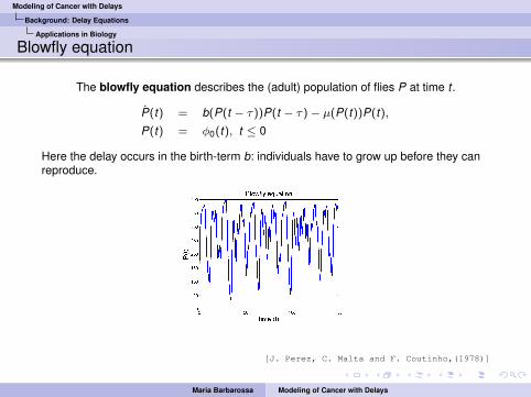
The blowfly equation describes the (adult) population of flies P at time t .
P(t) = b(P(t − τ))P(t − τ)− µ(P(t))P(t),
P(t) = φ0(t), t ≤ 0
Here the delay occurs in the birth-term b: individuals have to grow up before they canreproduce.
[J. Perez, C. Malta and F. Coutinho,(1978)]
Maria Barbarossa Modeling of Cancer with Delays
Modeling of Cancer with Delays
Background: Delay Equations
Stability Analysis for DDEs
Overview
1 Background: Delay EquationsOrdinary vs. Delay Differential EquationsApplications in BiologyStability Analysis for DDEs
2 Delay Equations for Tumor ModellingFew Different ModelsModels based on the cell cycleTime delays in the immune response
3 Conclusions
Maria Barbarossa Modeling of Cancer with Delays
Modeling of Cancer with Delays
Background: Delay Equations
Stability Analysis for DDEs
Linearization
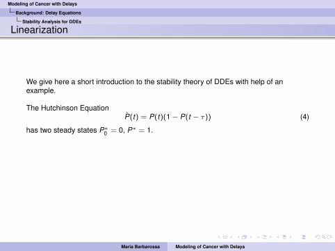
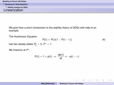
We give here a short introduction to the stability theory of DDEs with help of anexample.
The Hutchinson EquationP(t) = P(t)(1− P(t − τ)) (4)
has two steady states P∗0 = 0, P∗ = 1.
We linearize at P∗:
P(t) = 1 + p(t) ⇒dp(t)
dt≈ −p(t − τ).
Maria Barbarossa Modeling of Cancer with Delays
Modeling of Cancer with Delays
Background: Delay Equations
Stability Analysis for DDEs
Linearization
We give here a short introduction to the stability theory of DDEs with help of anexample.
The Hutchinson EquationP(t) = P(t)(1− P(t − τ)) (4)
has two steady states P∗0 = 0, P∗ = 1.
We linearize at P∗:
P(t) = 1 + p(t) ⇒dp(t)
dt≈ −p(t − τ).
Maria Barbarossa Modeling of Cancer with Delays
Modeling of Cancer with Delays
Background: Delay Equations
Stability Analysis for DDEs
Characteristic roots
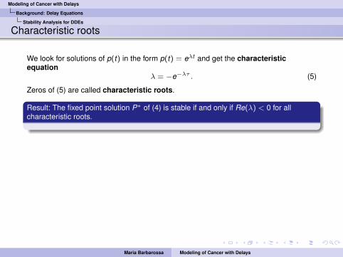
We look for solutions of p(t) in the form p(t) = eλt and get the characteristicequation
λ = −e−λτ . (5)
Zeros of (5) are called characteristic roots.
Result: The fixed point solution P∗ of (4) is stable if and only if Re(λ) < 0 for allcharacteristic roots.
Consider complex roots in the form λ = µ+ iω and separate the real part from theimaginary one in (5)
µ = −e−µτcos(ωτ) ω = e−µτsin(ωτ).
Stability is affected by the values of τ : stability loss when µ(τ) first crosses theimaginary axis. It can be shown that 0 < τ < π
2 is the condition for stability of P∗.For τ > π
2 the solution shows an oscillatory behavior.
[J.D. Murray,(2001)]
Maria Barbarossa Modeling of Cancer with Delays

Modeling of Cancer with Delays
Background: Delay Equations
Stability Analysis for DDEs
Characteristic roots
We look for solutions of p(t) in the form p(t) = eλt and get the characteristicequation
λ = −e−λτ . (5)
Zeros of (5) are called characteristic roots.
Result: The fixed point solution P∗ of (4) is stable if and only if Re(λ) < 0 for allcharacteristic roots.
Consider complex roots in the form λ = µ+ iω and separate the real part from theimaginary one in (5)
µ = −e−µτcos(ωτ) ω = e−µτsin(ωτ).
Stability is affected by the values of τ : stability loss when µ(τ) first crosses theimaginary axis. It can be shown that 0 < τ < π
2 is the condition for stability of P∗.For τ > π
2 the solution shows an oscillatory behavior.
[J.D. Murray,(2001)]
Maria Barbarossa Modeling of Cancer with Delays

Modeling of Cancer with Delays
Background: Delay Equations
Stability Analysis for DDEs
A general result by Cooke and Van den DriesscheMore in general, it is possible to reduce the characteristic polynomial to the form
P(λ) + Q(λ)e−λτ .
The following result holds:
Theorem
Let P and Q be analytic functions in a right half-plane Re(z) > −δ, with δ > 0. If thefollowing conditions are verified
P(z) and Q(z) have no common imaginary zero.
P(−iy) = P(iy) and Q(−iy) = Q(iy) for y ∈ R.
P(0) + Q(0) 6= 0.
F (y) ≡ |P(iy)|2 − |Q(iy)|2 for y ∈ R has at most a finite number of real zeros.
Then
If F (y) = 0 has no positive roots, the delay problem has the same stabilityproperties of the ODE problem, for all τ > 0.
If F (y) = 0 has at least one positive root and each positive root is simple, then asτ increases, stability switches may occur. There is a τ∗ such that the equation isalways unstable for τ > τ∗.
[K. Cooke, P. Van den Driessche (1986)]Maria Barbarossa Modeling of Cancer with Delays
Modeling of Cancer with Delays
Delay Equations for Tumor Modelling
Overview
1 Background: Delay Equations
2 Delay Equations for Tumor ModellingFew Different ModelsModels based on the cell cycleTime delays in the immune response
3 Conclusions
Maria Barbarossa Modeling of Cancer with Delays
Modeling of Cancer with Delays
Delay Equations for Tumor Modelling
Introduction
There are many reasons for time delays in tumor modelling:
Delays from regulation processes (e.g. it takes time for the cell to produce growthfactors or release toxins)
Delays due to the space description (e.g. nutrients take time to diffuse into thetumor)
Delays for the description of an event which “takes time” (e.g. length of theinterphase or length of mitotic phase)
Delays for the immune system which reacts “after a while”
We will see some examples for these different cases and spend some time with delaysrelated to the cell cycle.
Maria Barbarossa Modeling of Cancer with Delays

Modeling of Cancer with Delays
Delay Equations for Tumor Modelling
Few Different Models
Overview
1 Background: Delay EquationsOrdinary vs. Delay Differential EquationsApplications in BiologyStability Analysis for DDEs
2 Delay Equations for Tumor ModellingFew Different ModelsModels based on the cell cycleTime delays in the immune response
3 Conclusions
Maria Barbarossa Modeling of Cancer with Delays

Modeling of Cancer with Delays
Delay Equations for Tumor Modelling
Few Different Models
Burkowsky:a computer tool to predict the tumor growth
Assume to deal with an avascular solid tumor.
The tumoral mass is assumed to be a sphere. Tumor’s growth is related on theconcentration of oxygen(σ(r)), which varies depending on the distance from thesurface of the tumor. Below a certain oxygen concentration level σnec cell deathoccurs.
Decline in tumor growth also due to mitotic inhibitory effect of chemicals arisingfrom necrotic fragments.
During the final stages of tumor growth the tumoral sphere is made up ofconcentric shells (necrotic core, dormant cells, partially proliferating cells, freelyproliferating cells)
On entering the necrotic core a cell does not immediately expel inhibitorychemicals: such a phenomenon occurs after a time τ (the delay). Thus if anecrotic core is formed at time t , at any time t ≥ t + τ we assume the existence ofa necrotic sphere with radius rn(t − τ) surrounded by an outer layer of dead cellsawaiting lysis.
Results: If the delay τ is larger than zero, the tumor may experience a temporaryregression. Further conditions for an equilibrium in the tumor size were found.
[F. Burkowsky,(1977)]
Maria Barbarossa Modeling of Cancer with Delays
Modeling of Cancer with Delays
Delay Equations for Tumor Modelling
Few Different Models
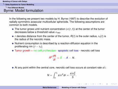
Byrne: Model formulation
In the following we present two models by H. Byrne (1997) to describe the evolution ofradially symmetric avascular multicellular spheroids. The following assumptions arecommon to both models.
The tumor grows until nutrient concentration (σ(r , t)) at the center of the tumordecreases below a threshold value σnec .
r denotes distance from the center of the tumor, R(t) is the outer radius, rn(t) isthe radius of the necrotic mass.
Nutrient consumption is described by a reaction-diffusion equation in theproliferating rim (r − rn).
Tumor growth = net cell proliferation - apoptotic cell loss - necrotic cell loss
R2 dRdt
= S − A − N.
At any point within the central core, necrotic cell loss occurs at constant rate sλ:
N =
Z rn
0sλr2dr =
sλr2n
3.
Maria Barbarossa Modeling of Cancer with Delays
Modeling of Cancer with Delays
Delay Equations for Tumor Modelling
Few Different Models
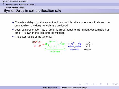
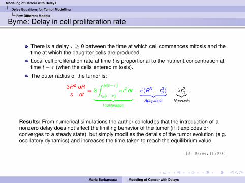
Byrne: Delay in cell proliferation rate
There is a delay τ ≥ 0 between the time at which cell commences mitosis and thetime at which the daughter cells are produced.
Local cell proliferation rate at time t is proportional to the nutrient concentration attime t − τ (when the cells entered mitosis).
The outer radius of the tumor is:
3R2
sdRdt
= 3Z R(t−τ)
rn(t−τ)σr2dr| {z }
Proliferation
− σ(R3 − r3n )| {z }
Apoptosis
− λr3n|{z}
Necrosis
.
Results: From numerical simulations the author concludes that the introduction of anonzero delay does not affect the limiting behavior of the tumor (if it explodes orconverges to a steady state), but simply modifies the details of the tumor evolution (e.g.oscillatory dynamics) and increases the time taken to reach the equilibrium value.
[H. Byrne,(1997)]
Maria Barbarossa Modeling of Cancer with Delays
Modeling of Cancer with Delays
Delay Equations for Tumor Modelling
Few Different Models
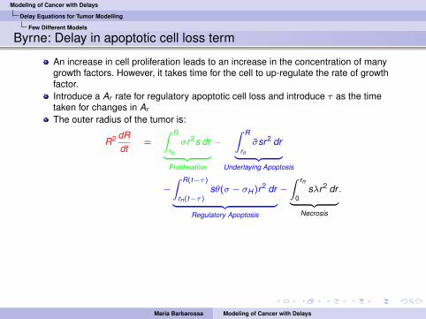
Byrne: Delay in apoptotic cell loss term
An increase in cell proliferation leads to an increase in the concentration of manygrowth factors. However, it takes time for the cell to up-regulate the rate of growthfactor.Introduce a Ar rate for regulatory apoptotic cell loss and introduce τ as the timetaken for changes in Ar
The outer radius of the tumor is:
R2 dRdt
=
Z R
rnσr2s dr| {z }
Proliferation
−Z R
rnσsr2 dr| {z }
Underlaying Apoptosis
−Z R(t−τ)
rn(t−τ)sθ(σ − σH )r2 dr| {z }
Regulatory Apoptosis
−Z rn
0sλr2 dr| {z }
Necrosis
.
Results: The introduction of a nonzero delay affects the tumor’s growth dynamics!Taking a parameter setting for which the ODE model (τ = 0) reaches a fixed point, theauthor shows that small delays lead to damped oscillations around the stationary point.For large delays the steady state is no longer stable: the tumor does not proliferate anymore and it turns into a necrotic mass.
[H. Byrne,(1997)]
Maria Barbarossa Modeling of Cancer with Delays

Modeling of Cancer with Delays
Delay Equations for Tumor Modelling
Few Different Models
Byrne: Delay in apoptotic cell loss term
An increase in cell proliferation leads to an increase in the concentration of manygrowth factors. However, it takes time for the cell to up-regulate the rate of growthfactor.Introduce a Ar rate for regulatory apoptotic cell loss and introduce τ as the timetaken for changes in Ar
The outer radius of the tumor is:
R2 dRdt
=
Z R
rnσr2s dr| {z }
Proliferation
−Z R
rnσsr2 dr| {z }
Underlaying Apoptosis
−Z R(t−τ)
rn(t−τ)sθ(σ − σH )r2 dr| {z }
Regulatory Apoptosis
−Z rn
0sλr2 dr| {z }
Necrosis
.
Results: The introduction of a nonzero delay affects the tumor’s growth dynamics!Taking a parameter setting for which the ODE model (τ = 0) reaches a fixed point, theauthor shows that small delays lead to damped oscillations around the stationary point.For large delays the steady state is no longer stable: the tumor does not proliferate anymore and it turns into a necrotic mass.
[H. Byrne,(1997)]
Maria Barbarossa Modeling of Cancer with Delays

Modeling of Cancer with Delays
Delay Equations for Tumor Modelling
Models based on the cell cycle
Overview
1 Background: Delay EquationsOrdinary vs. Delay Differential EquationsApplications in BiologyStability Analysis for DDEs
2 Delay Equations for Tumor ModellingFew Different ModelsModels based on the cell cycleTime delays in the immune response
3 Conclusions
Maria Barbarossa Modeling of Cancer with Delays

Modeling of Cancer with Delays
Delay Equations for Tumor Modelling
Models based on the cell cycle
The cell cycle
Maria Barbarossa Modeling of Cancer with Delays

Modeling of Cancer with Delays
Delay Equations for Tumor Modelling
Models based on the cell cycle
A good idea...
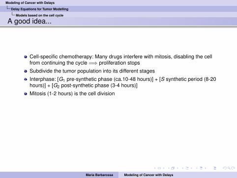
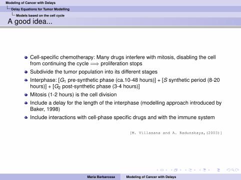
Cell-specific chemotherapy: Many drugs interfere with mitosis, disabling the cellfrom continuing the cycle =⇒ proliferation stops
Subdivide the tumor population into its different stages
Interphase: [G1 pre-synthetic phase (ca.10-48 hours)] + [S synthetic period (8-20hours)] + [G2 post-synthetic phase (3-4 hours)]
Mitosis (1-2 hours) is the cell division
Include a delay for the length of the interphase (modelling approach introduced byBaker, 1998)
Include interactions with cell-phase specific drugs and with the immune system
[M. Villasana and A. Radunskaya,(2003)]
Maria Barbarossa Modeling of Cancer with Delays

Modeling of Cancer with Delays
Delay Equations for Tumor Modelling
Models based on the cell cycle
A good idea...
Cell-specific chemotherapy: Many drugs interfere with mitosis, disabling the cellfrom continuing the cycle =⇒ proliferation stops
Subdivide the tumor population into its different stages
Interphase: [G1 pre-synthetic phase (ca.10-48 hours)] + [S synthetic period (8-20hours)] + [G2 post-synthetic phase (3-4 hours)]
Mitosis (1-2 hours) is the cell division
Include a delay for the length of the interphase (modelling approach introduced byBaker, 1998)
Include interactions with cell-phase specific drugs and with the immune system
[M. Villasana and A. Radunskaya,(2003)]
Maria Barbarossa Modeling of Cancer with Delays
Modeling of Cancer with Delays
Delay Equations for Tumor Modelling
Models based on the cell cycle
...but a wrong model
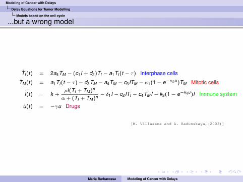
TI(t) = 2a4TM − (c1I + d2)TI − a1TI(t − τ) Interphase cells
TM (t) = a1TI(t − τ)− d3TM − a4TM − c3ITM − κ1(1− e−κ2u)TM Mitotic cells
I(t) = k +ρI(TI + TM )n
α+ (TI + TM )n− δ1I − c2ITI − c4TM I − k3(1− e−k4u)I Immune system
u(t) = −γu Drugs
[M. Villasana and A. Radunskaya,(2003)]
Maria Barbarossa Modeling of Cancer with Delays

Modeling of Cancer with Delays
Delay Equations for Tumor Modelling
Models based on the cell cycle
A more detailed model
Liu et al. introduce the quiescent phase and correct the model by Villasana:
[Liu et al.,(2007)]
Maria Barbarossa Modeling of Cancer with Delays
Modeling of Cancer with Delays
Delay Equations for Tumor Modelling
Models based on the cell cycle
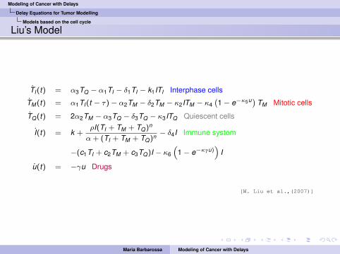
Liu’s Model
TI(t) = α3TQ − α1TI − δ1TI − k1ITI Interphase cells
TM (t) = α1TI(t − τ)− α2TM − δ2TM − κ2ITM − κ4`1− e−κ5u´TM Mitotic cells
TQ(t) = 2α2TM − α3TQ − δ3TQ − κ3ITQ Quiescent cells
I(t) = k +ρI(TI + TM + TQ)n
α+ (TI + TM + TQ)n− δ4I Immune system
−(c1TI + c2TM + c3TQ)I − κ6
“1− e−κ7u)
”I
u(t) = −γu Drugs
[W. Liu et al.,(2007)]
Maria Barbarossa Modeling of Cancer with Delays
Modeling of Cancer with Delays
Delay Equations for Tumor Modelling
Models based on the cell cycle
Liu’s Model: Analysis
The model was rescaled and new parameter were introduced (the biologicalmeaning goes a bit lost)
Model analysis at different stages: first the ODE model for tumor cells only (noimmune system, no drugs), then the delay model.
Stability analysis carried out by investigation of the characteristic polynomial.
Conditions for the stability of the tumor-free equilibrium were investigated.
[W. Liu et al.,(2007)]
Maria Barbarossa Modeling of Cancer with Delays

Modeling of Cancer with Delays
Delay Equations for Tumor Modelling
Models based on the cell cycle
Liu’s Model: Results
From the simple ODE model for tumor cells only, the author can show that theresting phase G0 controls cancer dynamics. Indeed if the “ingoing”-rate into theresting state is smaller than the rate of departure from the resting state, the tumorwill have more proliferating cells and grow.
The immune system can be able to control cancer growth and under certainconditions reduce its size.
When analysing the delay model, a stability switch due to τ can be found. When τis larger than a threshold value τ , the cancer-free equilibrium becomes unstable.A long delay in the interphase enables cells to avoid the treatment and reenter themitotic phase (and therefore proliferate!)
[W. Liu et al.,(2007)]
Maria Barbarossa Modeling of Cancer with Delays

Modeling of Cancer with Delays
Delay Equations for Tumor Modelling
Time delays in the immune response
Overview
1 Background: Delay EquationsOrdinary vs. Delay Differential EquationsApplications in BiologyStability Analysis for DDEs
2 Delay Equations for Tumor ModellingFew Different ModelsModels based on the cell cycleTime delays in the immune response
3 Conclusions
Maria Barbarossa Modeling of Cancer with Delays
Modeling of Cancer with Delays
Delay Equations for Tumor Modelling
Time delays in the immune response
General considerations
A further class of models deals with interactions of tumor cells with the cells of theimmune system.
These models are simplifications of the physiological phenomenon and considermainly the following two-populations dynamics:
tumor cells ≡ target cells ≡ preyimmune system cells ≡ effectors ≡ predators
Hypothesis of antitumoral immune surveillance (Burnet,1970): the immune systempatrols the cells of the body, and, upon recognition of a (group of) cell(s) that hasbecome cancerous, it will attempt to destroy it(them), thus preventing the growth ofsome tumors.
Maria Barbarossa Modeling of Cancer with Delays
Modeling of Cancer with Delays
Delay Equations for Tumor Modelling
Time delays in the immune response
Immunotherapy
Observed facts:
The immune system can, in some cases, eradicate the tumor.
The tumor may escape from the immune system control and grow.
An equilibrium is established: the tumor survives in a microscopic (steady) state.
Idea: do not treat the tumor but the immune system!
Immunotherapy focuses on the stimulation of the immune system:
cancer vaccine trains the immune system to recognize tumor cells as targets
manipulation of therapeutic antibodies stimulates the immune system to attackthe tumor
Aim: if it is not possible to eradicate the tumor, reduce its size to a life-compatibledimension.
Maria Barbarossa Modeling of Cancer with Delays

Modeling of Cancer with Delays
Delay Equations for Tumor Modelling
Time delays in the immune response
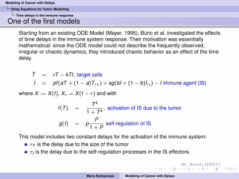
One of the first modelsStarting from an existing ODE Model (Mayer, 1995), Búric et al. investigated the effectsof time delays in the immune system response. Their motivation was essentiallymathematical: since the ODE model could not describe the frequently observed,irregular or chaotic dynamics, they introduced chaotic behavior as an effect of the timedelay.
T = rT − kTI, target cells
I = pf (aT + (1− a)TτT ) + sg(bI + (1− b)IτI )− I immune agent (IS)
where X := X(t), Xτ = X(t − τ) and with
f (T ) =T 4
1 + T 4, activation of IS due to the tumor
g(I) = pI3
1 + I3self-regulation of IS
This model includes two constant delays for the activation of the immune system:τT is the delay due to the size of the tumorτI is the delay due to the self-regulation processes in the IS effectors.
[N. Buric,(2001)]
Maria Barbarossa Modeling of Cancer with Delays
Modeling of Cancer with Delays
Delay Equations for Tumor Modelling
Time delays in the immune response
One of the first modelsStarting from an existing ODE Model (Mayer, 1995), Búric et al. investigated the effectsof time delays in the immune system response. Their motivation was essentiallymathematical: since the ODE model could not describe the frequently observed,irregular or chaotic dynamics, they introduced chaotic behavior as an effect of the timedelay.
T = rT − kTI, target cells
I = pf (aT + (1− a)TτT ) + sg(bI + (1− b)IτI )− I immune agent (IS)
where X := X(t), Xτ = X(t − τ) and with
f (T ) =T 4
1 + T 4, activation of IS due to the tumor
g(I) = pI3
1 + I3self-regulation of IS
This model includes two constant delays for the activation of the immune system:τT is the delay due to the size of the tumorτI is the delay due to the self-regulation processes in the IS effectors.
[N. Buric,(2001)]
Maria Barbarossa Modeling of Cancer with Delays

Modeling of Cancer with Delays
Delay Equations for Tumor Modelling
Time delays in the immune response
Buric’s results
The model was investigated essentially for one constant delay only (setting a = 1 orb = 1).Varying the parameter values, different dynamics were possible.
For a delay τT in f (T ) and fixed parameter values admitting a limit cycle in the ODEmodel, increasing the value of τT a periodic orbit is found (left). For large values of τTthe orbit becomes chaotic (left).
[N. Buric,(2001)]
Maria Barbarossa Modeling of Cancer with Delays

Modeling of Cancer with Delays
Delay Equations for Tumor Modelling
Time delays in the immune response
Predator-prey models by A. d’Onofrio
A. d’Onofrio worked from 2005 to a general class of predator-prey models fortumor-immune system interplay. The general model is an ODE system:
T = T (f (T )− φ(T , I)), tumor
I = β(T )I − µ(T )I + σq(T ) + θ(t) immune agent (IS)
f (T ) is a bounded, positive, non-growing function which describes the tumorgrowth
φ(T , I) is the loss of tumor cells due to the attack by the immune system
σq(T ), with q(0) = 1, represents the influx of immune cells in tumor in situ (maydepend on the tumor size)
β(T ) is a growing function of T and models the stimulating effect of the tumor onimmune cells proliferation
µ(T ) is the loss rate of effectors(IS) due to their interactions with the tumor
θ(t) models the immunotherapy (constant, periodic or absent).
[A. d’Onofrio,(2005)]
Maria Barbarossa Modeling of Cancer with Delays

Modeling of Cancer with Delays
Delay Equations for Tumor Modelling
Time delays in the immune response
Predator-prey models by A. d’OnofrioIn 2010 the basic ODE model was modified by including a delay for the immune systemresponse:
T = T (f (T )− φ(T , I)),
I = β(Tτ )I − µ(T )I + σq(T ) + θ(t).
Results:The stability of the disease-free equilibrium (T = 0) is not affected by the delay τConditions for the stability of the nontrivial equilibrium P := (T , I) were given andit was further shown that there is a critical value τ0 such that: P is stable if τ < τ0,P is unstable if τ > τ0 and a Hopf-Bifurcation occurs at τ = τ0 (here τ is thebifurcation parameter).
Here
T ≈ 10.925 and τ = 0.3(left plot), τ = 0.5 (central plot), τ = 1(right plot).
[A. d’Onofrio,(2010)]
Maria Barbarossa Modeling of Cancer with Delays

Modeling of Cancer with Delays
Delay Equations for Tumor Modelling
Time delays in the immune response
Predator-prey models by A. d’Onofrio
Interactions between delayed immune response and immunotherapy were investigated.The therapy was assumed to be ω-periodic
θ(t) = θAexp„−
1γ
„t − ω
—tω
�««where θA is the maximal ’boost’ for the influx of effectors, ω is the time between twoconsecutive deliveries and γ is a measure of decay time.Results:
Here: τ = 0.6:
In case of no therapy (left plot), γ = 40, ω = 0.1 (central plot), γ = 1.1, ω = 3(right plot).
[A. d’Onofrio,(2010)]
Maria Barbarossa Modeling of Cancer with Delays
Modeling of Cancer with Delays
Conclusions
Overview
1 Background: Delay Equations
2 Delay Equations for Tumor Modelling
3 Conclusions
Maria Barbarossa Modeling of Cancer with Delays

Modeling of Cancer with Delays
Conclusions
What did we learn?
Let us sum up the main ideas of today’s lecture:
Delay equations for a better description of the real-life phenomenon
Delay models better than ODE-models reproduce observed dynamics ormeasured data (e.g. oscillatory and chaotic behavior)
For the analysis of constant delay problems we can exploit the theory of ODEs
Numerical implementation is easier (and faster to compute) compared toPDE-problemsDelays in tumor modelling can arise from
the “spatiality” of the problemregulation processesactivation and reaction of the immune system
Maria Barbarossa Modeling of Cancer with Delays

Modeling of Cancer with Delays
Conclusions
What did we learn?
Let us sum up the main ideas of today’s lecture:
Delay equations for a better description of the real-life phenomenon
Delay models better than ODE-models reproduce observed dynamics ormeasured data (e.g. oscillatory and chaotic behavior)
For the analysis of constant delay problems we can exploit the theory of ODEs
Numerical implementation is easier (and faster to compute) compared toPDE-problems
Delays in tumor modelling can arise fromthe “spatiality” of the problemregulation processesactivation and reaction of the immune system
Maria Barbarossa Modeling of Cancer with Delays

Modeling of Cancer with Delays
Conclusions
What did we learn?
Let us sum up the main ideas of today’s lecture:
Delay equations for a better description of the real-life phenomenon
Delay models better than ODE-models reproduce observed dynamics ormeasured data (e.g. oscillatory and chaotic behavior)
For the analysis of constant delay problems we can exploit the theory of ODEs
Numerical implementation is easier (and faster to compute) compared toPDE-problemsDelays in tumor modelling can arise from
the “spatiality” of the problem
regulation processesactivation and reaction of the immune system
Maria Barbarossa Modeling of Cancer with Delays
Modeling of Cancer with Delays
Conclusions
What did we learn?
Let us sum up the main ideas of today’s lecture:
Delay equations for a better description of the real-life phenomenon
Delay models better than ODE-models reproduce observed dynamics ormeasured data (e.g. oscillatory and chaotic behavior)
For the analysis of constant delay problems we can exploit the theory of ODEs
Numerical implementation is easier (and faster to compute) compared toPDE-problemsDelays in tumor modelling can arise from
the “spatiality” of the problemregulation processes
activation and reaction of the immune system
Maria Barbarossa Modeling of Cancer with Delays
Modeling of Cancer with Delays
Conclusions
What did we learn?
Let us sum up the main ideas of today’s lecture:
Delay equations for a better description of the real-life phenomenon
Delay models better than ODE-models reproduce observed dynamics ormeasured data (e.g. oscillatory and chaotic behavior)
For the analysis of constant delay problems we can exploit the theory of ODEs
Numerical implementation is easier (and faster to compute) compared toPDE-problemsDelays in tumor modelling can arise from
the “spatiality” of the problemregulation processesactivation and reaction of the immune system
Maria Barbarossa Modeling of Cancer with Delays

Modeling of Cancer with Delays
Conclusions
References
References
R. Driver, Ordinary and Delay Differential Equations, Springer (1977).
A. Bellen, M. Zennaro,Numerical methods for delay differential equations Clarendon Press,(2003)
H. Byrne,The effect of time delays on the dynamics of avascular tumor growth, Math. Biosci.,Vol. 144 (1997)
C. Baker et al., Modelling and analysis of time-lags in some basic patterns of cell proliferation,J. Math. Biol. , Vol 37 (1998)
M. Villasana, A. Radunskaya, A delay differential equation model for tumor growth, J. Math.Bio., Vol. 47 (2003)
W. Liu et al., A mathematical model for M-phase specific chemotherapy including theG0-phase and immunoresponse, Math. Biosc. Engin., Vol. 4 (2007)
A. d’Onofrio et al., Delay-induced oscillatory dynamics of tumour-immune system interaction,Math. Comp. Mod., Vol.51 (2010)
Maria Barbarossa Modeling of Cancer with Delays


![Aquaporins as diagnostic and therapeutic targets in cancer ...cancer, Laryngeal cancer, Lung cancer [43], Nasopharyngeal cancer, Ovarian cancer [37] Tumor grade, prognosis, tumor angiogenesis,](https://img.pdfslide.us/doc/110x75/5ffa8fafa51a2a21db58011f/aquaporins-as-diagnostic-and-therapeutic-targets-in-cancer-cancer-laryngeal.jpg)