Deep Learning for Speech Recognition

Mark Gales

July 2017

Apple Siri (2011)

2/57

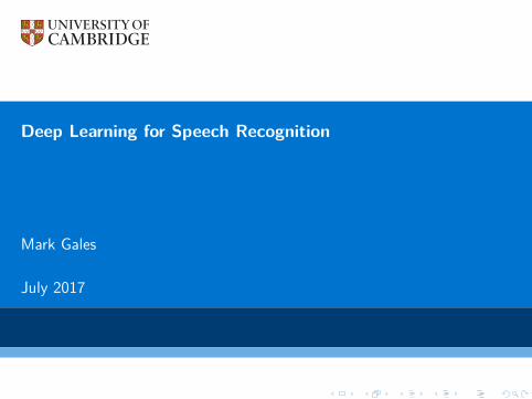
Speech Application Areas

3/57

Speech Processing:Proof of Concept

4/57

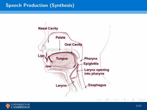
Speech Production (Synthesis)

5/57

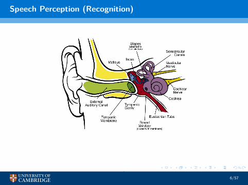
Speech Perception (Recognition)

6/57

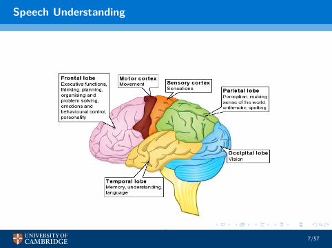
Speech Understanding

7/57

Should Speech Recognisers have Ears?

8/57

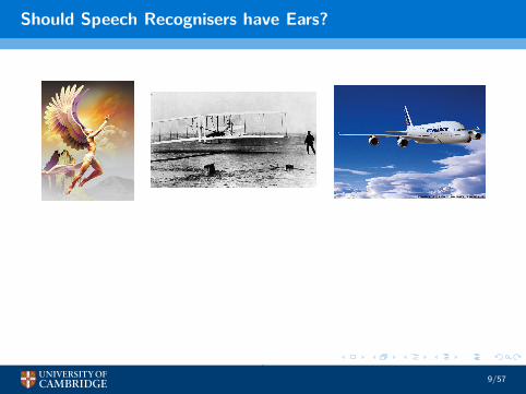
Should Speech Recognisers have Ears?

No - I’m and Engineer!

9/57

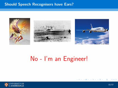
Should Speech Recognisers have Ears?

No - I’m an Engineer!

10/57

Speech Recognition

11/57

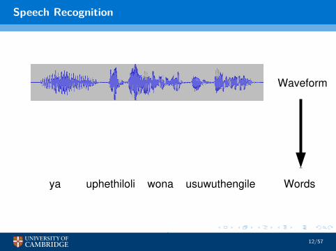
Speech Recognition

/w/−/O/+/n/ Context−Dependent

Wordsusuwuthengileuphethiloliya wona

Waveform

Phones

Phones

Features

/w/ /O/ /n/ /a/

12/57

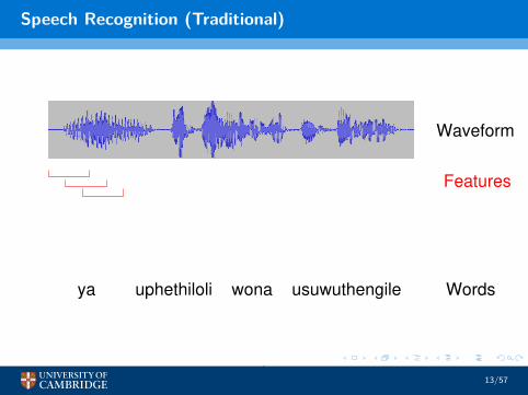
Speech Recognition (Traditional)

usuwuthengileuphethiloliya wona

Waveform

Phones

Phones

Features

/w/ /O/ /n/ /a/

Context−Dependent

Words

/w/−/O/+/n/

13/57

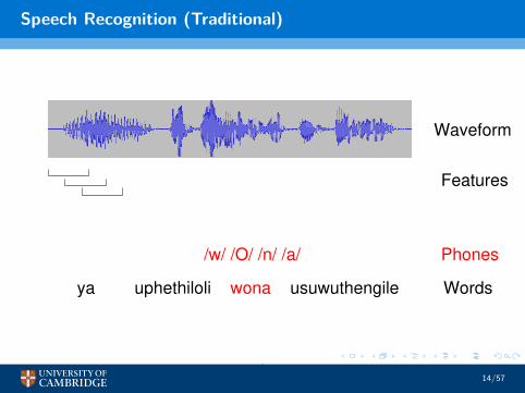
Speech Recognition (Traditional)

usuwuthengileuphethiloliya

Waveform

Phones

Phones

Features

/w/ /O/ /n/ /a/

Context−Dependent

Words

/w/−/O/+/n/

wona

14/57

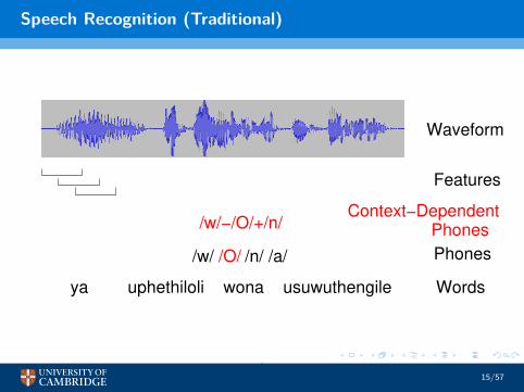
Speech Recognition (Traditional)

usuwuthengileuphethiloliya

Waveform

Phones

Phones

Features

Wordswona

/n/ /a//O//w/

/w/−/O/+/n/Context−Dependent

15/57

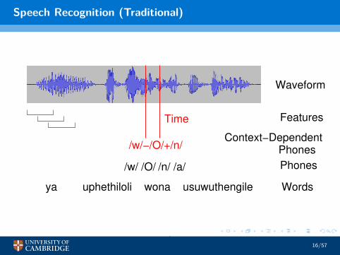
Speech Recognition (Traditional)

usuwuthengileuphethiloliya

Waveform

Phones

Phones

Features

Wordswona

/n/ /a//O//w/

/w/−/O/+/n/

Time

Context−Dependent

16/57

Sequence-to-Sequence Modelling

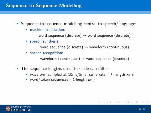
• Sequence-to-sequence modelling central to speech/language:• machine translation:

word sequence (discrete) → word sequence (discrete)• speech synthesis:

word sequence (discrete) → waveform (continuous)• speech recognition:

waveform (continuous) → word sequence (discrete)

• The sequence lengths on either side can differ• waveform sampled at 10ms/5ms frame-rate - T -length x1∶T• word/token sequences - L-length ω1∶L

17/57

Speech Recognition Framework (Traditional)

LanguageModel

Waveform

ya uphe...Features Decoder

AcousticModel

Lexicon

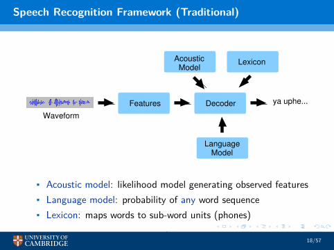
• Acoustic model: likelihood model generating observed features• Language model: probability of any word sequence• Lexicon: maps words to sub-word units (phones)

18/57

Generative Models [2, 3]

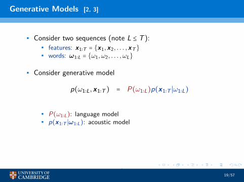
• Consider two sequences (note L ≤ T ):• features: x1∶T = {x1,x2, . . . ,xT}• words: ω1∶L = {ω1, ω2, . . . , ωL}

• Consider generative model

p(ω1∶L,x1∶T ) = P(ω1∶L)p(x1∶T ∣ω1∶L)

• P(ω1∶L): language model• p(x1∶T ∣ω1∶L): acoustic model

19/57

Language Model: N-grams [15]

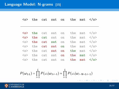
<s> the cat sat on the mat </s>

<s> the cat sat on the mat </s><s> the cat sat on the mat </s><s> the cat sat on the mat </s><s> the cat sat on the mat </s><s> the cat sat on the mat </s><s> the cat sat on the mat </s><s> the cat sat on the mat </s>

P(ω1∶L) =L∏

i=1P(ωi ∣ω1∶i−1) ≈

L∏

i=1P(ωi ∣ωi−N+1∶i−1)

20/57

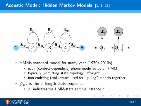
Acoustic Model: Hidden Markov Models [1, 8, 23]

33a

22 44

2 3 4 51a

12a

23a

34a

a

45

at xt+1

t t+1φ φ

x

• HMMs standard model for many year (1970s-2010s)• each (context-dependent) phone modelled by an HMM• typically 3-emitting state topology, left-right• non-emitting (end) states used for “gluing” models together

• φ1∶T is the T -length state-sequence• φt indicates the HMM-state at time instance t

21/57

Acoustic Model: HMMs [1, 8]

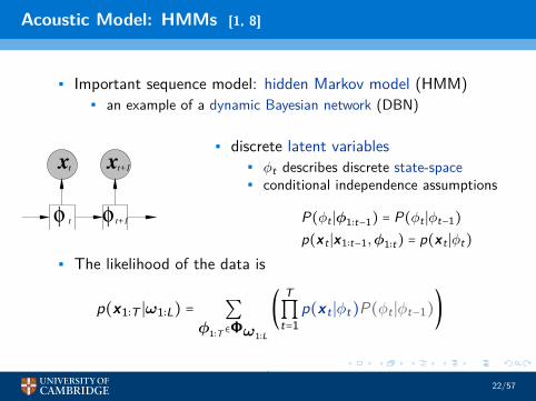
• Important sequence model: hidden Markov model (HMM)• an example of a dynamic Bayesian network (DBN)

t xt+1

t t+1φ φ

x

• discrete latent variables• φt describes discrete state-space• conditional independence assumptions

P(φt ∣φ1∶t−1) = P(φt ∣φt−1)p(xt ∣x1∶t−1,φ1∶t) = p(xt ∣φt)

• The likelihood of the data is

p(x1∶T ∣ω1∶L) = ∑

φ1∶T ∈Φω1∶L

(

T∏

t=1p(xt ∣φt)P(φt ∣φt−1))

22/57

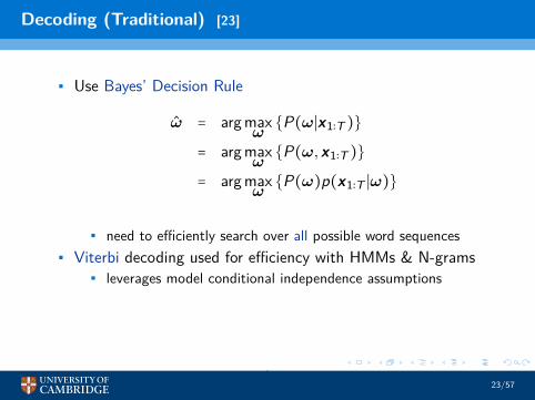
Decoding (Traditional) [23]

• Use Bayes’ Decision Rule

ω̂ = argmaxω{P(ω∣x1∶T )}

= argmaxω{P(ω,x1∶T )}

= argmaxω{P(ω)p(x1∶T ∣ω)}

• need to efficiently search over all possible word sequences• Viterbi decoding used for efficiency with HMMs & N-grams

• leverages model conditional independence assumptions

23/57

Deep Learning andRecurrent Neural Networks

24/57

What is Deep Learning?

From Wikipedia:Deep learning is a branch of machine learning based on aset of algorithms that attempt to model high-levelabstractions in data by using multiple processing layers,with complex structures or otherwise, composed ofmultiple non-linear transformations.

25/57

What is Deep Learning?

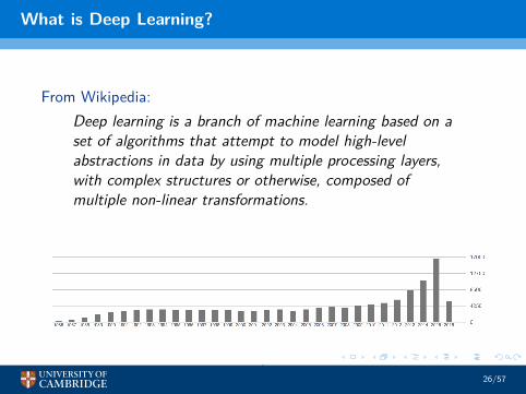
From Wikipedia:Deep learning is a branch of machine learning based on aset of algorithms that attempt to model high-levelabstractions in data by using multiple processing layers,with complex structures or otherwise, composed ofmultiple non-linear transformations.

26/57

Deep Neural Networks [13]

y(x)x

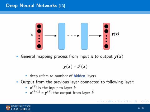
• General mapping process from input x to output y(x)

y(x) = F(x)

• deep refers to number of hidden layers• Output from the previous layer connected to following layer:

• x(k) is the input to layer k• x(k+1) = y(k) the output from layer k

27/57

Neural Network Layer/Node

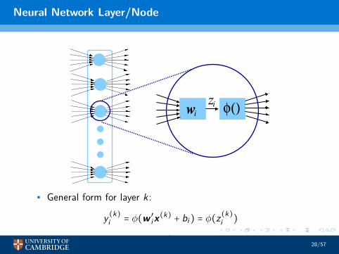
φ()wi

zi

• General form for layer k:

y (k)i = φ(w ′ix(k) + bi) = φ(z(k)i )

28/57

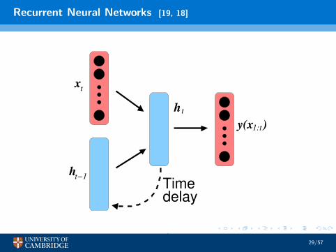
Recurrent Neural Networks [19, 18]

tx

t−1h

t

Time

h

delay

1:ty(x )

29/57

Recurrent Neural Networks

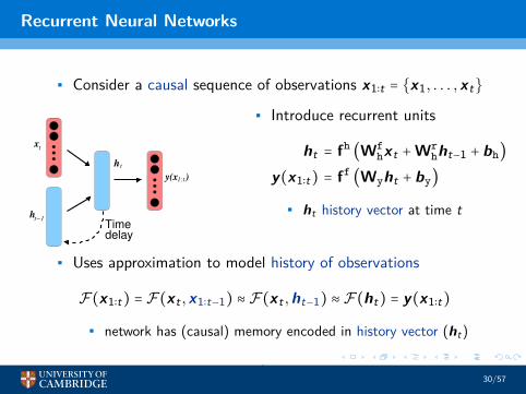
• Consider a causal sequence of observations x1∶t = {x1, . . . ,xt}

tx

t−1h

t

Time

h

delay

1:ty(x )

• Introduce recurrent units

ht = fh(Wf

hxt +Wrhht−1 + bh)

y(x1∶t) = ff(Wyht + by)

• ht history vector at time t

• Uses approximation to model history of observations

F(x1∶t) = F(xt ,x1∶t−1) ≈ F(xt ,ht−1) ≈ F(ht) = y(x1∶t)

• network has (causal) memory encoded in history vector (ht)

30/57

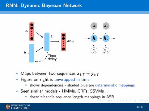
RNN: Dynamic Bayesian Network

tx

t−1h

t

Time

h

delay

1:ty(x )

xt+1xt

ht t+1h

yt yt+1

• Maps between two sequences x1∶T → y1∶T• Figure on right is unwrapped in time

• shows dependencies - shaded blue are deterministic mappings• Seen similar models - HMMs, CRFs, SSVMs ..

• doesn’t handle sequence length mappings in ASR

31/57

RNN: Variants and Extensions [21, 6, 14, 11, 22, 7]

• Extensions of standard RNN structure:• bi-directional RNN (depends on future and past)• latent-variable RNNs (continuous latent variables)

• Modification to the recurrent units (gating)• long-short term memory units (LSTMs)• gated recurrent units (GRUs)• highway connections (gating in time)

32/57

Acoustic Modelling

33/57

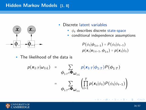
Hidden Markov Models [1, 8]

t xt+1

t t+1φ φ

x

• Discrete latent variables• φt describes discrete state-space• conditional independence assumptions

P(φt ∣φ1∶t−1) = P(φt ∣φt−1)p(xt ∣x1∶t−1,φ1∶t) = p(xt ∣φt)

• The likelihood of the data is

p(x1∶T ∣ω1∶L) = ∑

φ1∶T ∈Φω1∶L

p(x1∶T ∣φ1∶T )P(φ1∶T )

= ∑

φ1∶T ∈Φω1∶L

(

T∏

t=1p(xt ∣φt)P(φt ∣φt−1))

34/57

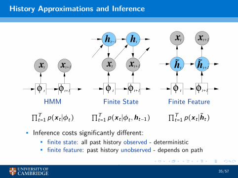
History Approximations and Inference

t xt+1

t t+1φ φ

x

φ φ

xt xt+1

ht−1 th

t t+1 φ φ

xt xt+1

th~

ht+1

~

t t+1

HMM Finite State Finite Feature

∏Tt=1 p(xt ∣φt) ∏

Tt=1 p(xt ∣φt ,ht−1) ∏

Tt=1 p(xt ∣h̃t)

• Inference costs significantly different:• finite state: all past history observed - deterministic• finite feature: past history unobserved - depends on path

35/57

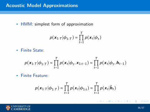
Acoustic Model Approximations

• HMM: simplest form of approximation

p(x1∶T ∣φ1∶T ) ≈T∏

t=1p(xt ∣φt)

• Finite State:

p(x1∶T ∣φ1∶T ) ≈T∏

t=1p(xt ∣φt ,x1∶t−1) ≈

T∏

t=1p(xt ∣φt ,ht−1)

• Finite Feature:

p(x1∶T ∣φ1∶T ) ≈T∏

t=1p(xt ∣φ1∶t) ≈

T∏

t=1p(xt ∣h̃t)

36/57

“Likelihoods” [3]

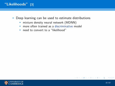
• Deep learning can be used to estimate distributions• mixture density neural network (MDNN)• more often trained as a discriminative model• need to convert to a “likelihood”

37/57

“Likelihoods” [3]

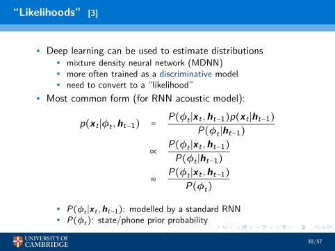
• Deep learning can be used to estimate distributions• mixture density neural network (MDNN)• more often trained as a discriminative model• need to convert to a “likelihood”

• Most common form (for RNN acoustic model):

p(xt ∣φt ,ht−1) =

P(φt ∣xt ,ht−1)p(xt ∣ht−1)P(φt ∣ht−1)

∝

P(φt ∣xt ,ht−1)P(φt ∣ht−1)

≈

P(φt ∣xt ,ht−1)P(φt)

• P(φt ∣xt ,ht−1): modelled by a standard RNN• P(φt): state/phone prior probability

38/57

“Baseline” Acoustic Training Criteria

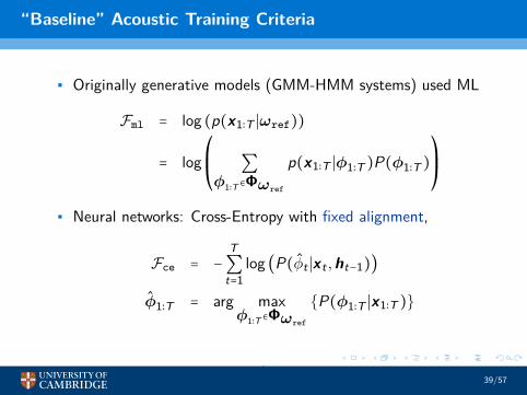
• Originally generative models (GMM-HMM systems) used ML

Fml = log (p(x1∶T ∣ωref))

= log⎛

⎜

⎝

∑

φ1∶T ∈Φωref

p(x1∶T ∣φ1∶T )P(φ1∶T )⎞

⎟

⎠

• Neural networks: Cross-Entropy with fixed alignment,

Fce = −

T∑

t=1log (P(φ̂t ∣xt ,ht−1))

φ̂1∶T = arg maxφ1∶T ∈Φωref

{P(φ1∶T ∣x1∶T )}

39/57

Example “Generative” Acoustic Model [20]

understand the CLDNN architecture are presented in Section 4. Re-sults on the larger data sets are then discussed in Section 5. Finally,Section 6 concludes the paper and discusses future work.

2. MODEL ARCHITECTURE

This section describes the CLDNN architecture shown in Figure 1.

2.1. CLDNN

Frame xt, surrounded by l contextual vectors to the left and r con-textual vectors to the right, is passed as input to the network. Thisinput is denoted as [xt�l, . . . , xt+r]. In our work, each frame xt isa 40-dimensional log-mel feature.

First, we reduce frequency variance in the input signal by pass-ing the input through a few convolutional layers. The architectureused for each CNN layer is similar to that proposed in [2]. Specif-ically, we use 2 convolutional layers, each with 256 feature maps.We use a 9x9 frequency-time filter for the first convolutional layer,followed by a 4x3 filter for the second convolutional layer, and thesefilters are shared across the entire time-frequency space. Our pool-ing strategy is to use non-overlapping max pooling, and pooling infrequency only is performed [11]. A pooling size of 3 was used forthe first layer, and no pooling was done in the second layer.

The dimension of the last layer of the CNN is large, due to thenumber of feature-maps⇥time⇥frequency context. Thus, we add alinear layer to reduce feature dimension, before passing this to theLSTM layer, as indicated in Figure 1. In [12] we found that addingthis linear layer after the CNN layers allows for a reduction in pa-rameters with no loss in accuracy. In our experiments, we found thatreducing the dimensionality, such that we have 256 outputs from thelinear layer, was appropriate.

After frequency modeling is performed, we next pass the CNNoutput to LSTM layers, which are appropriate for modeling the sig-nal in time. Following the strategy proposed in [3], we use 2 LSTMlayers, where each LSTM layer has 832 cells, and a 512 unit projec-tion layer for dimensionality reduction. Unless otherwise indicated,the LSTM is unrolled for 20 time steps for training with truncatedbackpropagation through time (BPTT). In addition, the output statelabel is delayed by 5 frames, as we have observed with DNNs thatinformation about future frames helps to better predict the currentframe. The input feature into the CNN has l contextual frames tothe left and r to the right, and the CNN output is then passed to theLSTM. In order to ensure that the LSTM does not see more than 5frames of future context, which would increase the decoding latency,we set r = 0 for CLDNNs.

Finally, after performing frequency and temporal modeling, wepass the output of the LSTM to a few fully connected DNN layers.As shown in [5], these higher layers are appropriate for producing ahigher-order feature representation that is more easily separable intothe different classes we want to discriminate. Each fully connectedlayer has 1,024 hidden units.

2.2. Multi-scale Additions

The CNN takes a long-term feature, seeing a context of t�l to t (i.e.,r = 0 in the CLDNN), and produces a higher order representationof this to pass into the LSTM. The LSTM is then unrolled for 20timesteps, and thus consumes a larger context of 20 + l. However,we feel there is complementary information in also passing the short-term xt feature to the LSTM. In fact, the original LSTM work in[3] looked at modeling a sequence of 20 consecutive short-term xt

C

...

D

D

L

L

Cconvolutional

layers

LSTMlayers

fullyconnected

layers

output targets

[xt-l,..., xt, ...., xt+r]

linearlayer

dimred

(1)

xt

(2)

Fig. 1. CLDNN Architecture

features, with no context. In order to model short and long-termfeatures, we take the original xt and pass this as input, along withthe long-term feature from the CNN, into the LSTM. This is shownby dashed stream (1) in Figure 1.

The use of short and long-term features in a neural network hasbeen explored previously (i.e., [13, 14]). The main difference be-tween previous work and ours is that we are able to do this jointlyin one network, namely because of the power of the LSTM sequen-tial modeling. In addition, our combination of short and long-termfeatures results in a negligible increase in the number of networkparameters.

In addition, we explore if there is complementarity betweenmodeling the output of the CNN temporally with an LSTM, as wellas discriminatively with a DNN. Specifically, motivated by work incomputer vision [10], we explore passing the output of the CNN intoboth the LSTM and DNN. This is indicated by the dashed stream(2) in Figure 1. This idea of combining information from CNN andDNN layers has been explored before in speech [11, 15], thoughprevious work added extra DNN layers to do the combination. Ourwork differs in that we pass the output of the CNN directly into theDNN, without extra layers and thus minimal parameter increase.

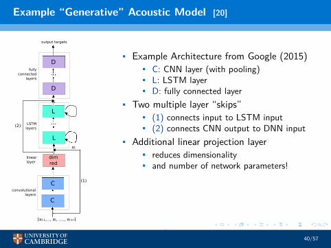
• Example Architecture from Google (2015)• C: CNN layer (with pooling)• L: LSTM layer• D: fully connected layer

• Two multiple layer “skips”• (1) connects input to LSTM input• (2) connects CNN output to DNN input

• Additional linear projection layer• reduces dimensionality• and number of network parameters!

40/57

Discriminative Models(“End-to-End” Models)

41/57

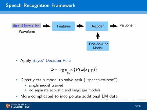
Speech Recognition Framework

Waveform

ya uphe...

ModelEnd−to−End

Features Decoder

• Apply Bayes’ Decision Rule

ω̂ = argmaxω{P(ω∣x1∶T )}

• Directly train model to solve task (“speech-to-text”)• single model trained• no separate acoustic and language models

• More complicated to incorporate additional LM data

42/57

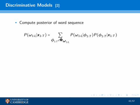
Discriminative Models [2]

• Compute posterior of word sequence

P(ω1∶L∣x1∶T ) = ∑

φ1∶T ∈Φω1∶L

P(ω1∶L∣φ1∶T )P(φ1∶T ∣x1∶T )

43/57

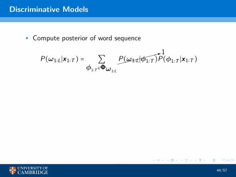
Discriminative Models

• Compute posterior of word sequence

P(ω1∶L∣x1∶T ) = ∑

φ1∶T ∈Φω1∶L

������

�:1P(ω1∶L∣φ1∶T )P(φ1∶T ∣x1∶T )

44/57

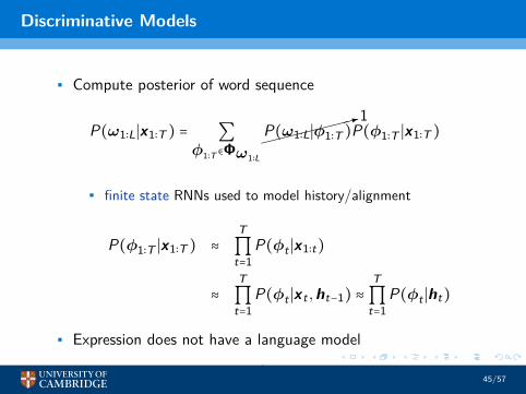
Discriminative Models

• Compute posterior of word sequence

P(ω1∶L∣x1∶T ) = ∑

φ1∶T ∈Φω1∶L

������

�:1P(ω1∶L∣φ1∶T )P(φ1∶T ∣x1∶T )

• finite state RNNs used to model history/alignment

P(φ1∶T ∣x1∶T ) ≈

T∏

t=1P(φt ∣x1∶t)

≈

T∏

t=1P(φt ∣xt ,ht−1) ≈

T∏

t=1P(φt ∣ht)

• Expression does not have a language model

45/57

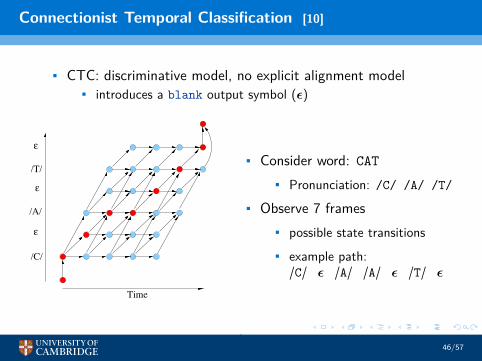
Connectionist Temporal Classification [10]

• CTC: discriminative model, no explicit alignment model• introduces a blank output symbol (ε)

/C/

Time

ε

ε

ε

/T/

/A/

• Consider word: CAT

• Pronunciation: /C/ /A/ /T/

• Observe 7 frames• possible state transitions• example path:/C/ ε /A/ /A/ ε /T/ ε

46/57

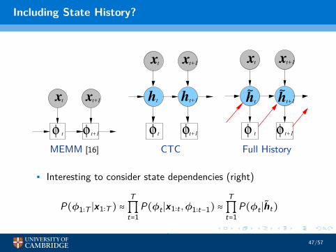
Including State History?

t xt+1

t t+1φ φ

x

t+1

tφ

ht+1

t+1φ

th

xt x

φ φ

xt xt+1

th~

ht+1

~

t t+1

MEMM [16] CTC Full History

• Interesting to consider state dependencies (right)

P(φ1∶T ∣x1∶T ) ≈T∏

t=1P(φt ∣x1∶t ,φ1∶t−1) ≈

T∏

t=1P(φt ∣h̃t)

47/57

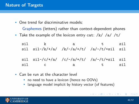
Nature of Targets

• One trend for discriminative models:Graphemes (letters) rather than context-dependent phones

• Take the example of the lexicon entry cat: /k/ /a/ /t/

sil k a t silsil sil-/k/+/a/ /k/-/a/+/t/ /a/-/t/+sil sil

sil sil-/c/+/a/ /c/-/a/+/t/ /a/-/t/+sil silsil c a t sil

• Can be run at the character level• no need to have a lexicon (hence no OOVs)• language model implicit by history vector (of features)

48/57

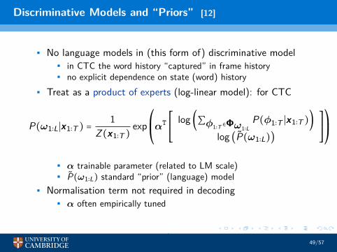
Discriminative Models and “Priors” [12]

• No language models in (this form of) discriminative model• in CTC the word history “captured” in frame history• no explicit dependence on state (word) history

• Treat as a product of experts (log-linear model): for CTC

P(ω1∶L∣x1∶T ) =1

Z(x1∶T )exp⎛

⎜

⎝

αT⎡⎢⎢⎢⎢⎣

log (∑φ1∶T ∈Φω1∶LP(φ1∶T ∣x1∶T ))

log (P̃(ω1∶L))

⎤⎥⎥⎥⎥⎦

⎞

⎟

⎠

• α trainable parameter (related to LM scale)• P̃(ω1∶L) standard “prior” (language) model

• Normalisation term not required in decoding• α often empirically tuned

49/57

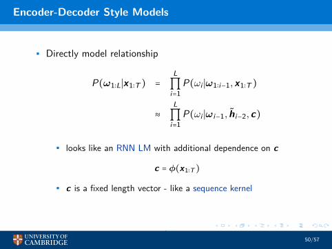
Encoder-Decoder Style Models

• Directly model relationship

P(ω1∶L∣x1∶T ) =

L∏

i=1P(ωi ∣ω1∶i−1,x1∶T )

≈

L∏

i=1P(ωi ∣ωi−1, h̃i−2, c)

• looks like an RNN LM with additional dependence on c

c = φ(x1∶T )

• c is a fixed length vector - like a sequence kernel

50/57

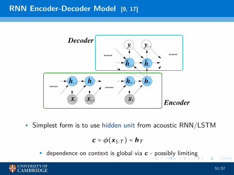
RNN Encoder-Decoder Model [9, 17]

xt+1

th

xT

hTT−1h

xt

ht−1

i+1yi y

hi−1 ih~ ~

Decoder

Encoder

• Simplest form is to use hidden unit from acoustic RNN/LSTM

c = φ(x1∶T ) = hT

• dependence on context is global via c - possibly limiting

51/57

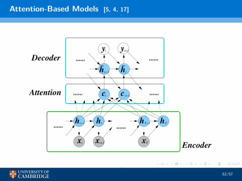
Attention-Based Models [5, 4, 17]

Decoder

Attention ci+1ic

xt+1

th

xT

hTT−1h

xt

ht−1

Encoder

i+1yi y

hi−1 ih~ ~

52/57

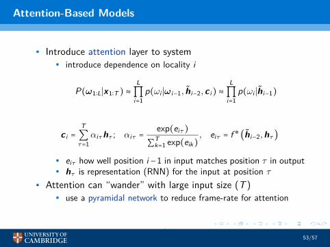
Attention-Based Models

• Introduce attention layer to system• introduce dependence on locality i

P(ω1∶L∣x1∶T ) ≈L∏

i=1p(ωi ∣ωi−1, h̃i−2, c i) ≈

L∏

i=1p(ωi ∣h̃i−1)

c i =T∑

τ=1αiτ hτ ; αiτ =

exp(eiτ)∑

Tk=1 exp(eik)

, eiτ = f e(h̃i−2,hτ)

• eiτ how well position i −1 in input matches position τ in output• hτ is representation (RNN) for the input at position τ

• Attention can “wander” with large input size (T )• use a pyramidal network to reduce frame-rate for attention

53/57

Conclusions

54/57

Deep Learning and Speech Recognition

It’s an interesting time!

• Deep learning integrated into standard speech toolkits• Kaldi, HTK etc

• Rich variety of models and topologies supported by:• large quantities of training data• GPU-based training (and parallel implementations)• array of software tools: TensorFlow, CNTK, Theano ...

• Most state-of-the-art still “generative”• but next conference in August ...

55/57

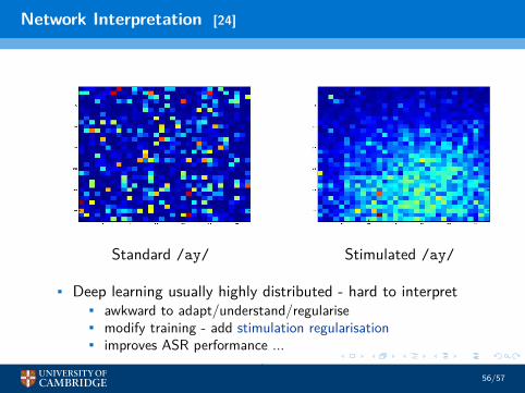
Network Interpretation [24]

Standard /ay/ Stimulated /ay/

• Deep learning usually highly distributed - hard to interpret• awkward to adapt/understand/regularise• modify training - add stimulation regularisation• improves ASR performance ...

56/57

Thank-you!

57/57

[1] L. Baum and J. Eagon, “An Inequality with Applications to Statistical Estimation for Probabilistic Functionsof Markov Processes and to a Model for Ecology,” Bull Amer Math Soc, vol. 73, pp. 360–363, 1967.

[2] C. M. Bishop, Pattern Recognition and Machine Learning. Springer Verlag, 2006.

[3] H. Bourlard and N. Morgan, “Connectionist speech recognition: A hybrid approach,” 1994.

[4] W. Chan, N. Jaitly, Q. V. Le, and O. Vinyals, “Listen, attend and spell,” CoRR, vol. abs/1508.01211, 2015.[Online]. Available: http://arxiv.org/abs/1508.01211

[5] J. Chorowski, D. Bahdanau, D. Serdyuk, K. Cho, and Y. Bengio, “Attention-based models for speechrecognition,” CoRR, vol. abs/1506.07503, 2015. [Online]. Available: http://arxiv.org/abs/1506.07503

[6] J. Chung, C. Gulcehre, K. Cho, and Y. Bengio, “Empirical evaluation of gated recurrent neural networks onsequence modeling,” arXiv preprint arXiv:1412.3555, 2014.

[7] J. Chung, K. Kastner, L. Dinh, K. Goel, A. C. Courville, and Y. Bengio, “A recurrent latent variable modelfor sequential data,” CoRR, vol. abs/1506.02216, 2015. [Online]. Available:http://arxiv.org/abs/1506.02216

[8] M. Gales and S. Young, “The application of hidden Markov models in speech recognition,” Foundations andTrends in Signal Processing, vol. 1, no. 3, 2007.

[9] A. Graves, “Sequence transduction with recurrent neural networks,” CoRR, vol. abs/1211.3711, 2012.[Online]. Available: http://arxiv.org/abs/1211.3711

[10] A. Graves, S. Fernández, F. Gomez, and J. Schmidhuber, “Connectionist temporal classification: labellingunsegmented sequence data with recurrent neural networks,” in Proceedings of the 23rd internationalconference on Machine learning. ACM, 2006, pp. 369–376.

[11] A. Graves, A.-R. Mohamed, and G. Hinton, “Speech recognition with deep recurrent neural networks,” in2013 IEEE international conference on acoustics, speech and signal processing. IEEE, 2013, pp. 6645–6649.

[12] G. E. Hinton, “Products of experts,” in Proceedings of the Ninth International Conference on ArtificialNeural Networks (ICANN 99), 1999, pp. 1–6.

57/57

[13] G. Hinton, L. Deng, D. Yu, G. E. Dahl, A.-R. Mohamed, N. Jaitly, A. Senior, V. Vanhoucke, P. Nguyen,T. N. Sainath, et al., “Deep neural networks for acoustic modeling in speech recognition: The shared views offour research groups,” IEEE Signal Processing Magazine, vol. 29, no. 6, pp. 82–97, 2012.

[14] S. Hochreiter and J. Schmidhuber, “Long short-term memory,” Neural Comput., vol. 9, no. 8, pp.1735–1780, Nov. 1997.

[15] F. Jelinek, Statistical methods for speech recognition, ser. Language, speech, and communication.Cambridge (Mass.), London: MIT Press, 1997.

[16] H.-K. Kuo and Y. Gao, “Maximum entropy direct models for speech recognition,” IEEE Transactions AudioSpeech and Language Processing, 2006.

[17] L. Lu, X. Zhang, K. Cho, and S. Renals, “A study of the recurrent neural network encoder-decoder for largevocabulary speech recognition,” in Proc. INTERSPEECH, 2015.

[18] T. Robinson and F. Fallside, “A recurrent error propagation network speech recognition system,” ComputerSpeech & Language, vol. 5, no. 3, pp. 259–274, 1991.

[19] D. E. Rumelhart, G. E. Hinton, and R. J. Williams, “Parallel distributed processing: Explorations in themicrostructure of cognition, vol. 1,” D. E. Rumelhart, J. L. McClelland, and C. PDP Research Group, Eds.Cambridge, MA, USA: MIT Press, 1986, ch. Learning Internal Representations by Error Propagation, pp.318–362.

[20] T. N. Sainath, O. Vinyals, A. Senior, and H. Sak, “Convolutional, long short-term memory, fully connecteddeep neural networks,” in 2015 IEEE International Conference on Acoustics, Speech and Signal Processing(ICASSP). IEEE, 2015, pp. 4580–4584.

[21] M. Schuster and K. K. Paliwal, “Bidirectional recurrent neural networks,” IEEE Transactions on SignalProcessing, vol. 45, no. 11, pp. 2673–2681, 1997.

[22] R. K. Srivastava, K. Greff, and J. Schmidhuber, “Highway networks,” CoRR, vol. abs/1505.00387, 2015.[Online]. Available: http://arxiv.org/abs/1505.00387

[23] A. Viterbi, “Error bounds for convolutional codes and an asymptotically optimum decoding algorithm,”vol. 13, no. 2, pp. 260–269, 1967.

57/57

[24] C. Wu, P. Karanasou, M. Gales, and K. C. Sim, “Stimulated deep neural network for speech recognition,” inProceedings interspeech, 2016.

57/57