Embed Size (px)
Citation preview

Linear Gaussian Models for
Speech Recognition
Antti-Veikko Ilmari Rosti
Wolfson College
May 2004
Dissertation submitted to the University of Cambridge
for the degree of Doctor of Philosophy

ii
Declaration
This dissertation is the result of my own work and includes nothing which is the outcome of work
done in collaboration. It has not been submitted in whole or in part for a degree at any other
university. Some of the work has been published previously in conference proceedings [114,
118], a journal article [117] and technical reports [113, 115, 116]. The length of this thesis
including appendices, bibliography, footnotes, tables and equations is approximately 38,000
words and it contains 31 figures.

iii
Abstract
Currently the most popular acoustic model for speech recognition is the hidden Markov model
(HMM). However, HMMs are based on a series of assumptions, some of which are known to be
poor. In particular, the assumption that successive speech frames are conditionally independent
given the discrete state that generated them is not a good assumption for speech recognition.
State space models may be used to address some shortcomings of this assumption. State space
models are based on a continuous state vector evolving through time according to a state evo-
lution process. The observations are then generated by an observation process, which maps the
current continuous state vector onto the observation space. In this work, the state evolution and
observation processes are assumed to be linear and noise sources are distributed according to
Gaussians or Gaussian mixture models. Two forms of state evolution processes are considered.
First, the state evolution process is assumed to be piece-wise constant. All the variations of
the state vector about these constant values are modelled as noise. Using this approximation,
a new acoustic model called the factor analysed HMM (FAHMM) is presented. In the FAHMM
a discrete Markov random variable chooses the continuous state and the observation process
parameters. The FAHMM generalises a number of standard covariance models such as the inde-
pendent factor analysis, shared factor analysis and semi-tied covariance matrix HMMs. Efficient
training and recognition algorithms for the FAHMMs are presented along with speech recogni-
tion results using various configurations.
Second, the state evolution process is assumed to be a linear first-order Gauss-Markov ran-
dom process. Using Gaussian distributed noise sources and a factor analysis observation process
this model corresponds to a linear dynamical system (LDS). For acoustic modelling a discrete
Markov random variable is required to choose the LDS parameters. This hybrid model is called
the switching linear dynamical system (SLDS). The SLDS is related to the stochastic segment
model, which assumes that the segments are independent. In contrast, for the SLDS the contin-
uous state vector is propagated over the segment boundaries, thus providing a better model for
co-articulation. Unfortunately, exact inference for the SLDS is intractable due to the exponential
growth of posterior components in time. In this work, approximate methods based on both de-
terministic and stochastic algorithms are described. An efficient proposal mechanism for Gibbs
sampling is introduced along with application to parameter optimisation and N-best rescoring.
The results of medium vocabulary speech recognition experiments are presented.
Keywords: Speech recognition, acoustic modelling, hidden Markov models, state space mod-
els, linear dynamical systems, expectation maximisation, Markov chain Monte Carlo methods

iv
Acknowledgements
I would like to thank my supervisor Mark Gales for his guidance throughout my time as a PhD
research student in Cambridge. His expert advice and confidence in my research have been
invaluable, and I have learnt much on machine learning and speech recognition from him. It
has been a privilege to work with Mark.
I am indebted to Phil Woodland and Steve Young for leading the Speech Group and the Ma-
chine Intelligence Laboratory (formerly known as the Speech, Vision and Robotics Group). The
Laboratory provides truly outstanding facilities and a positive atmosphere for research thanks
to all of the students and staff working there. I am also grateful to Thomas Hain and Gunnar
Evermann for useful discussions and advice on the hidden Markov model toolkit. I must also
thank our systems administrators Patrick Gosling and Anna Langley for maintaining the stacks of
computers so I could run my experiments without difficulty. This work made use of equipment
kindly supplied by IBM under an SUR award.
I am grateful to the Cambridge European Trust, the Engineering and Physical Sciences Re-
search Council, the Finnish Cultural Foundation, the Jenny and Antti Wihuri Foundation, the
Nokia Foundation, the Research Scholarship Foundation of Tampere, the Tampere Chamber of
Commerce and Industry, and the Tampere Graduate School in Information Science and Engineer-
ing for their financial support. I must thank Jaakko Astola and Visa Koivunen for their assistance
in securing the funding. Without them I could never have realised my dream of studying in
Cambridge.
I must also thank Judy-Ann for putting up with my countless hours in front of the computer
and showing me her unfaltering love. Special thanks go to Nigel Kettley for proofreading this
dissertation, and finally thanks are due to friends and family who have always been there for
me.

v
Abbreviations
DARPA Defence Advanced Research Projects Agency
DBN Dynamic Bayesian network
EM Expectation maximisation
FAHMM Factor analysed hidden Markov model
GMM Gaussian mixture model
GSFA Global shared factor analysis
HLDA Heteroscedastic linear discriminant analysis
HMM Hidden Markov model
HTK Hidden Markov model toolkit
IFA Independent factor analysis
KL distance Kullback-Leibler distance
LDA Linear discriminant analysis
LDS Linear dynamical system
LVCSR Large vocabulary continuous speech recognition
MCMC Markov chain Monte Carlo
MFCC Mel-frequency cepstral coefficient
ML Maximum likelihood
MLLR Maximum likelihood linear regression
MLSS Maximum likelihood state sequence
NIST National Institute of Standards and Technology
PLP Perceptual linear prediction
RBGS Rao-Blackwellised Gibbs sampling
RM corpus Resource Management corpus
SFA Shared factor analysis
SLDS Switching linear dynamical system
SSM Stochastic segment model
STC Semi-tied covariance matrix
SWB corpus Switchboard corpus
VTLN Vocal tract length normalisation
WER Word error rate

vi
Mathematical Notation
A matrix of arbitrary dimensions
A′ transpose of matrix A
A−1 inverse of matrix A
|A| determinant of matrix A
x vector of arbitrary dimensions
xj jth scalar element of x
p(x) probability density function of continuous variable x
x(n) nth sample drawn from p(x)
P (q = j) discrete probability of event q = j, probability mass function
p(x|q = j) conditional density function of x given event q = j
Ex|q = j expected value of x given event q = j
N (µ,Σ) multivariate Gaussian distribution with mean vector µ and covariance matrix Σ
N (x;µ,Σ) likelihood value for vector x assuming it is Gaussian distributed
General Model Notation
θ set of arbitrary model parameters
θ set of estimated model parameters
θ(k) set of model parameters at kth iteration
Q(θ,θ(k)) auxiliary function for arbitrary θ and fixed θ(k)
η number of model parameters
Ns number of discrete states
M (x) number of GMM components in state space
M (o) number of GMM components in observation space
cjn GMM weight associated with state j and component n
µjn GMM mean vector associated with state j and component n
Σjn GMM covariance matrix associated with state j and component n
Σ(x)jn GMM covariance matrix associated with state j and state space
component n
Σ(o)jm GMM covariance matrix associated with state j and observation
space component m
Cj observation matrix associated with state j
Q sequence of discrete states
q−t sequence of discrete states, qt not included, q1, . . . , qt−1, qt+1, . . . , qT
X sequence of continuous state vectors
O sequence of speech observation vectors
ot tth speech observation vector
o1:t partial observation sequence from 1 to t, o1, . . . ,ot
W sequence of words

vii
HMM and FAHMM Notation
aij discrete state transition probability
bj(ot) observation density associated with state j
αj(t) forward variable associated with state j at time t
βi(t) backward variable associated with state i at time t
γj(t) posterior probability of state j given O
γjn(t) posterior probability of state j and GMM component n given O
γjmn(t) posterior probability of state j, state space and observation space GMM
components n and m given O
µjmn GMM mean vector associated with state j, state space and observation
space GMM components n and m given O
Σjmn GMM covariance matrix associated with state j, state space and observation
space GMM components n and m given O
xjmnt estimated state vector associated with state j, state space and observation
space GMM components n and m at time t given O
Rjmnt estimated state correlation matrix associated with state j, state space and
observation space GMM components n and m at time t given O
LDS and SLDS Notation
µ(i) initial state mean vector
Σ(i) initial state covariance matrix
Aj continuous state evolution matrix associated with state j
xt+1|t Kalman predictor mean vector
Σt+1|t Kalman predictor covariance matrix
xt|t Kalman filter mean vector
Σt|t Kalman filter covariance matrix
xt Kalman smoother mean vector
Σt Kalman smoother covariance matrix
Σt,t+1 Kalman smoother cross-covariance matrix
P−1t|t backward information filter matrix
P−1t|t mt|t backward information filter vector
P−1t|t+1 backward information predictor matrix
P−1t|t+1mt|t+1 backward information predictor vector
Contents
List of Figures xii
List of Tables xv
1 Introduction 1
1.1 Detailed Organisation of Thesis 3
2 Statistical Framework for Speech Recognition 4
2.1 Speech Recognition Systems 4
2.2 Standard Front-Ends 5
2.3 Hidden Markov Models 7
2.3.1 Generative Model of HMM 7
2.3.2 Maximum Likelihood Parameter Estimation 8
2.3.3 Baum-Welch Algorithm 9
2.3.4 Bayesian Learning 11
2.3.5 Discriminative Training 12
2.4 Speech Recognition Using HMMs 12
2.4.1 Recognition Units 12
2.4.2 Language Models 14
2.4.3 Recognition Algorithms 15
2.4.4 Scoring and Confidence 16
2.4.5 Normalisation and Adaptation 16
2.5 Covariance and Precision Modelling 18
2.5.1 Covariance Matrix Modelling 18
2.5.2 Precision Matrix Modelling 20
2.6 Segment Models 21
2.6.1 Stochastic Segment Model 21
2.6.2 Hidden Dynamic Models 22
viii

ix
2.7 Summary 23
3 Generalised Linear Gaussian Models 24
3.1 State Space Models 24
3.2 Bayesian Networks 25
3.3 State Evolution Process 27
3.3.1 Piece-Wise Constant State Evolution 27
3.3.2 Linear Continuous State Evolution 28
3.4 Observation Process 29
3.4.1 Factor Analysis 29
3.4.2 Linear Discriminant Analysis 30
3.5 Standard Linear Gaussian Models 32
3.5.1 Static Models 32
3.5.2 Example: Factor Analysis 33
3.5.3 Dynamic Models 34
3.5.4 Example: Linear Dynamical System 35
3.5.5 Higher-Order State Evolution in LDS 38
3.6 Summary 39
4 Learning and Inference in Linear Gaussian Models 40
4.1 Learning in Linear Gaussian Models 40
4.1.1 Lower Bound on Log-Likelihood 41
4.1.2 Expectation Maximisation Algorithm 42
4.1.3 Gaussian Mixture Model Example 43
4.2 Inference in Linear Gaussian Models 44
4.3 Approximate Inference: Deterministic Algorithms 45
4.3.1 Kullback-Leibler Distance 45
4.3.2 Moment Matching 46
4.3.3 Expectation Propagation 47
4.3.4 Variational Methods 48
4.4 Approximate Inference: Stochastic Algorithms 49
4.4.1 Monte Carlo Methods 49
4.4.2 Markov Chain Monte Carlo Methods 51
4.5 Summary 52
5 Piece-Wise Constant State Evolution 54
5.1 Factor Analysed Hidden Markov Models 54
5.1.1 Generative Model of FAHMM 54
5.1.2 FAHMM Likelihood Calculation 55
5.1.3 Optimising FAHMM Parameters 57
5.1.4 Standard Systems Related to FAHMMs 59

x
5.2 Implementation Issues 61
5.2.1 Initialisation 61
5.2.2 Parameter Sharing 62
5.2.3 Numerical Accuracy 64
5.2.4 Efficient Two Level Training 64
5.3 Summary 66
6 Linear Continuous State Evolution 67
6.1 Switching Linear Dynamical System 67
6.1.1 Generative Model of SLDS 68
6.1.2 Inference and Training 69
6.1.3 Approximate Inference and Learning 71
6.2 Rao-Blackwellised Gibbs Sampling 73
6.2.1 Efficient Proposal Distribution for SLDS 74
6.2.2 Gaussian Mixture Models in SLDS 75
6.2.3 RBGS in Speech Recognition 76
6.2.4 SLDS Initialisation 76
6.2.5 Parameter Optimisation 77
6.3 Summary 79
7 Experimental Evaluation 80
7.1 FAHMM Experiments 80
7.1.1 Resource Management 80
7.1.2 Minitrain 82
7.1.3 Hub5 68 Hour 84
7.1.4 Observation Matrix Tying 85
7.1.5 Varying State Space Dimensionality 86
7.2 SLDS Experiments 87
7.2.1 Single State System Training 88
7.2.2 Single State System Results 89
7.2.3 Three State System Results 93
7.2.4 Second-Order State Evolution 94
7.3 Summary 96
8 Conclusions 97
8.1 Summary 97
8.2 Future Work 100
A Resource Management Corpus and Baseline System 102

xi
B Useful Results from Matrix Algebra 103
B.1 Some Results on Sums of Matrices 103
B.2 Some Results on Partitioned Matrices 104
B.2.1 Application to Conditional Multivariate Gaussians 104
C Parameter Optimisation for GMM 106
C.1 Auxiliary Function 106
C.2 Parameter Update Formulae 107
C.2.1 Mixture Component Priors 107
C.2.2 Mixture Distribution Parameters 108
D Parameter Optimisation for FAHMM 109
D.1 Evaluation of Posterior Statistics 109
D.1.1 Forward-Backward Algorithm 110
D.1.2 Discrete State Posterior Probabilities 111
D.1.3 Continuous State Posterior Statistics 111
D.2 Transition Probability Update Formulae 112
D.3 Observation Space Parameter Update Formulae 113
D.3.1 Observation Matrix 113
D.3.2 Observation Noise Component Priors 114
D.3.3 Observation Noise Parameters 114
D.4 State Space Parameter Update Formulae 115
D.4.1 State Noise Component Priors 115
D.4.2 State Noise Parameters 116
E Kalman Filtering, Smoothing and Information Forms 118
E.1 Kalman Filter 118
E.2 Kalman Smoother 120
E.3 Forward Information Filter 121
E.4 Backward Information Filter 123
E.5 Two Filter Formulae for Kalman Smoothing 124
F Parameter Optimisation for LDS 126
F.1 Observation Space Parameter Update Formulae 126
F.2 State Space Parameter Update Formulae 127
F.3 Initial State Distribution Parameter Update Formulae 128
G Gibbs Sampling for SLDS 130
G.1 Proposal Distribution 130

List of Figures
2.1 General speech recognition system. 5
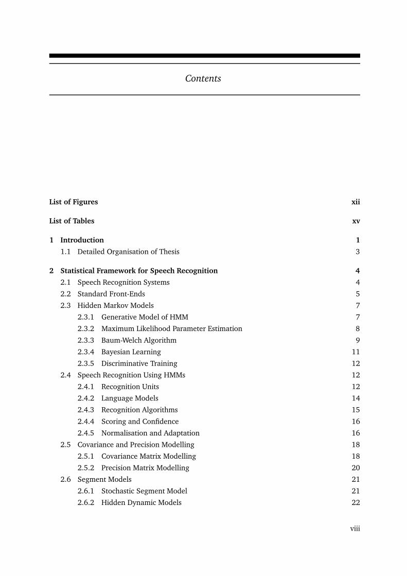
2.2 Acoustic front-end processing using overlapping window functions on speech
waveform. 6
2.3 Hidden Markov model generating observation vectors. 7
2.4 Example of single Gaussian triphones before and after state clustering. 13
2.5 Example of a phonetic decision tree for triphone models (from [130]). 14
2.6 Example of a binary regression tree for MLLR speaker adaptation. 17
3.1 Examples of Bayesian networks representing different assumptions on conditional
independence. 1) No independence assumptions between continuous random
variables z, x and o (shading denotes observable), 2) random variable o is condi-
tionally independent of z given x, 3) discrete random variable qt+1 is condition-
ally independent of all its predecessors given qt (discrete Markov chain). 25
3.2 Dynamic Bayesian network representing a hidden Markov model. 26
3.3 Trajectories of a state vector element illustrating different dynamic state evolution
processes. The piece-wise constant state evolution on the left hand side is based
on a HMM. The linear continuous state evolution on the right hand side is based
on a first-order Gauss-Markov random process. 27
3.4 An example illustrating factor analysis. The lower dimensional state vectors, xt,
are stretched and rotated by the observation matrix, C t, in the observation space.
This is convolved with the observation noise distribution to produce the final
distribution. 30
3.5 An example illustrating linear discriminant analysis. The black equal probability
contours represent two classes which are not separable in the original space. LDA
finds a projection down to one dimensional space, x1, with maximum between
class and minimum within class distance. 31
3.6 Diagram of static linear Gaussian models. The arrows represent additional prop-
erties to the model they are attached to. 32
xii

LIST OF FIGURES xiii
3.7 Bayesian network representing a standard factor analysis model. 33
3.8 Dynamic linear Gaussian models and how they relate to some of the static models. 35
3.9 Dynamic Bayesian network representing a standard linear dynamical system. 36
3.10 Dynamic Bayesian networks representing a model with second-order state evolu-
tion and an equivalent LDS with extended state space. 38
4.1 Log-likelihood function and lower bounds during three EM iterations with dif-
ferent initial values, m(1)1 = 7 and m
(1)1 = −2. The new estimates m
(k+1)1 tend
towards the nearest local maximum. 43
4.2 Assumed density filtering and expectation propagation in the Bayesian learning
example for the mean of a Gaussian mixture model. Two different orderings of
the observations in ADF result in the estimates θ(1) and θ(2). The EP algorithm
arrives at a good estimate provided it converges at all due to the multimodal
posterior. 47
4.3 Variational Bayes and importance sampling in the Bayesian learning example for
the mean of a Gaussian mixture model. Two different prior mean values, m = −2
and m = 0, in variational Bayes result in different estimates, θ(1) and θ(2). The
importance sampling is not challenged by the multimodal posterior distribution. 49
4.4 Gibbs sampling example for 8 full iterations. The initial value of the sample
is x(0) = [3,−3]′. The dashed line follows all the sampling steps, [x(0)1 , x
(0)2 ]′,
[x(1)1 , x
(0)2 ]′, [x
(1)1 , x
(1)2 ]′, [x
(2)1 , x
(1)2 ]′, . . .. 52
5.1 Dynamic Bayesian network representing a factor analysed hidden Markov model. 55
5.2 Auxiliary function values versus within iterations during 3 full iterations of two
level FAHMM training. 64
5.3 Average log-likelihood of the training data against the number of full iterations
for baseline HMM and an untied FAHMM with k = 13. One level training and
more efficient two level training with 10 within iterations were used. 65
6.1 Dynamic Bayesian networks representing a FAHMM and SLDS. 69
6.2 The posterior mean and variance of the first state vector element for an utterance
“What’s the overall re[source...]”. 70
6.3 True and estimated trajectories of the first Mel-frequency cepstral coefficient for
an utterance “What’s the overall re[source...]”. 71
6.4 Example iteration of Gibbs sampling for utterance “what”. 77
7.1 The word error rate against the state space dimensionality on the Hub5 68h
FAHMM experiments. 86
7.2 Average log-likelihood of the training data against the number of iterations. 89

LIST OF FIGURES xiv
7.3 Word error rate for the 1200 utterance test data against the number of hypothe-
ses for the 39-dimensional SLDS with fixed aligned N -best rescoring. Since a dif-
ferent system was used to produce the N -best lists, a larger number of hypotheses
than 50 should be used to obtain independent results. 91
7.4 Average of maximum log-likelihood for feb89 data set with 100 hypotheses against
the number of Gibbs sampling iterations. The highest log-likelihoods are mostly
obtained within the first 5 iterations. 93

List of Tables
5.1 Standard systems related to FAHMMs. FAHMM can be converted to the systems
on the left hand side by applying the restrictions on the right. 60
5.2 Number of free parameters per HMM and FAHMM state, η, usingM (x) state space
components, M (o) observation noise components and no sharing of individual
FAHMM parameters. Both diagonal covariance and full covariance matrix HMMs
are shown. 63
7.1 Word error rates (%) and number of free parameters per state, η, on the RM
task (1200 utterances), versus number of mixture components for the observation
pdfs, for HMM, STC and GSFA systems. 81
7.2 Word error rates (wer%) and number of free parameters per state, η, for the
baseline HMM systems with M (o) components. 82
7.3 Word error rates (%) and number of free parameters per state, η, on the Minitrain
task, versus number of mixture components for the observation and state space
pdfs, for FAHMM system with k = 13. 83
7.4 Word error rates (%) and number of free parameters per state, η, on the Hub5
68 hour task, versus number of mixture components for the observation pdfs, for
HMM, STC, SFA and GSFA systems with k = 13. SFA is a FAHMM with a single
state space mixture component, M (x) = 1. SFA has state specific observation
matrices whereas STC and GSFA have global ones. 84
7.5 Word error rates (%), number of free parameters per state, η, and average log-
likelihood scores, ll, on training data on the Hub5 68 hour task for 12-component
HMM, STC, GSFA, 65SFA and SFA systems with k = 13. 85
7.6 Number of free parameters per model and full decoding results for the 13 and
39-dimensional single and two observation noise component baseline FAHMMs
on the 1200 utterance test set and 300 utterance train set. 90
xv

LIST OF TABLES xvi
7.7 The “oracle – idiot” word error rates for the 13 and 39-dimensional baseline FAH-
MMs. These give the limits for the word error rates that may be obtained by
rescoring the corresponding 100-best lists. 90
7.8 Fixed alignment 100-best rescoring word error rates for the single state SLDS
systems trained with fixed alignments, and MLSS using Ni = 5 Gibbs sampling
iterations. 91
7.9 Fixed alignment 100-best rescoring word error rates for the single state SSM sys-
tems trained with fixed alignments, and MLSS using Ni = 5 Gibbs sampling iter-
ations. 92
7.10 Number of free parameters per state for the three state HMM, FAHMM, SLDS and
SSM. 94
7.11 100-best rescoring results in the feb89 set for the three state systems and fixed
alignment training. Oracle: 0.12 (M = 1), 0.08 (M = 2). Idiot: 51.78 (M = 1),
51.43 (M = 2). 94
7.12 Number of free parameters per state and 100-best rescoring word error rates for
the 13-dimensional (p = 13) three state systems and fixed alignment training.
Oracle: 1.18 (test), 0.08 (train). Idiot: 63.43 (test), 52.45 (train). 95

1
Introduction
Automatic speech recognition systems are currently available for various tasks. These tasks
range from voice dialling to desktop dictation. However, transcription of conversational speech
is still far from mature. In the 2002 NIST Rich Transcription evaluations of English conversa-
tional telephone speech, the best word error rates were as high as 23.9% [49]. These evaluation
systems typically use multiple passes, and very complex acoustic and language models in recog-
nition. This can result in computational complexity of more than 300 times real-time using a
1GHz Pentium III. The faster systems, less than 10 times real-time, achieved 27.2% using an
AMD Athlon XP 1900+ [49]. Although there are many aspects related to this type of recogni-
tion task, the poor performance, despite the highly complex models, suggests that there may
be inherent deficiencies in the modelling paradigm. This work concentrates on the problems
associated with acoustic modelling.
The Hidden Markov model (HMM) [62] is the most popular and successful choice of acoustic
model in modern speech recognisers. However, the HMM is based on assumptions which are not
appropriate for modelling speech signals [37, 60]. These assumptions include the following:
• Speech may be split into discrete states in which the speech waveform is assumed to be
stationary. Transitions between these states are assumed to be instantaneous;
• The probability of an acoustic vector corresponding to the current state depends only on
the vector and the current state. Thus, the acoustic vector is conditionally independent
of the sequence of acoustic vectors preceding and following the current vector given the
state.
In order to compensate for the first assumption, a model having many states would be desirable.
However, obtaining reliable estimates of the model parameters in such a system is a serious
problem. In practical systems the number of states may be up to 100,000. Thus, tying of the state
conditional observation density parameters is often used extensively. The second assumption is
not valid for speech signals due to the dynamic constraints caused by the physical attributes
of articulators and the use of overlapping frames in speech parameterisation. A popular way
to address this problem is to use acoustic vectors which include information over a time span
1

CHAPTER 1. INTRODUCTION 2
of several frames. This is usually achieved by appending the first and second-order regression
coefficients into the acoustic vectors. However, despite greatly enhancing the speech recognition
performance, mathematically this technique conflicts with the independence assumption. This
independence assumption is widely thought to be the major drawback of the use of HMMs for
speech recognition (eg. [24, 37, 60, 102, 105]).
State space models may be used to address the shortcomings of HMM based speech recog-
nition. State space models are based on a hidden continuous state evolution process and an
observation process which maps the current continuous state vector onto the observation space.
This work considers forms of state space models known as generalised linear Gaussian models
[113, 119]. In linear Gaussian models the state evolution and observation processes are based
on linear functions and Gaussian distributed noise sources. Linear Gaussian models are popular
as many forms may be trained efficiently using the expectation maximisation (EM) algorithm
[21]. This work generalises these models to include Gaussian mixture models as the noise
sources. The observation process in this work will be assumed to be based on factor analysis,
although linear discriminant analysis may also be viewed as an alternative observation process
[35]. This work may be divided in two parts depending on the form of state evolution process.
First, a model based on piece-wise constant state evolution process is described. This model
is called the factor analysed HMM (FAHMM). Here a standard diagonal covariance Gaussian
mixture HMM is used to generate the state vectors. While the discrete state associated with the
HMM remains the same, the state vector statistics are constant. Thus, the FAHMM does not
address the independence assumption. However, it generalises many standard covariance mod-
elling schemes such as the shared factor analysis [48] and semi-tied covariance matrix HMMs
[34]. Algorithms to optimise the FAHMM parameters and to use FAHMMs for speech recognition
are presented together with various schemes to improve their efficiency.
Second, a model based on linear first-order Gauss-Markov state evolution process is de-
scribed. This model is called the switching linear dynamical system (SLDS). The standard linear
dynamical system [66] is a linear Gaussian model based on this form of state evolution process
and factor analysis observation process. In the SLDS, standard linear dynamical system param-
eters are selected by an underlying discrete variable with Markovian dynamics. The SLDS is
closely related to the stochastic segment model (SSM) [24]. In the SSM the segments are as-
sumed to be independent of one another. At segment boundaries the state vector is initialised
based on the initial state distribution. However, in the SLDS the state vector is propagated
over the segment boundaries which should provide a better model for co-articulation. Unfor-
tunately, exact inference for the SLDS is intractable and approximate methods have to be con-
sidered. In this work the parameter optimisation and N -best rescoring algorithms are based
on Rao-Blackwellised Gibbs sampling (RBGS). The application of RBGS in speech recognition is
described along with an efficient proposal mechanism for sampling.

CHAPTER 1. INTRODUCTION 3
1.1 Detailed Organisation of Thesis
The next chapter introduces speech recognition systems in a statistical framework. The baseline
system, using hidden Markov models as the acoustic model, is described. Chapter 3 begins by
presenting generalised linear Gaussian models in a state space model framework. Possible state
evolution processes are reviewed and then different observation processes are discussed. Factor
analysis and linear dynamical system are used as examples of standard linear Gaussian mod-
els. Bayesian networks are used to illustrate the conditional independence assumptions made in
these models. The learning and inference algorithms for linear Gaussian models are presented
in Chapter 4. The EM algorithm is an efficient approach for maximum likelihood parameter
estimation in these models. Approximate inference algorithms in models for which the exact
inference is intractable are then introduced. The advantages and disadvantages of both deter-
ministic and stochastic algorithms are discussed. Chapter 5 describes factor analysed hidden
Markov models in detail. This is a generalised linear Gaussian model based on a piece-wise con-
stant state evolution process. Likelihood calculation and parameter optimisation are presented
together with the practical implementation issues. A model based on linear continuous state
evolution process called the switching linear dynamical system is introduced in Chapter 6. The
issues of inference in these forms of models are discussed. Possible approximate algorithms are
reviewed. A stochastic algorithm chosen for approximate inference is introduced together with
practical implementation issues in speech recognition. Experimental evaluation of the models is
carried out in Chapter 7. The thesis ends with conclusions and a discussion on potential future
work.
A description of the Resource Management corpus and the baseline HMM system are pre-
sented in Appendix A. A collection of useful mathematical results and derivations are presented
in the remaining appendices. Appendix B reviews some useful matrix algebra and an application
to conditional multivariate Gaussians. A derivation of the EM algorithm for a Gaussian mixture
model, factor analysed HMM and linear dynamical system are presented in Appendices C, D
and F, respectively. The parameter optimisation for the FAHMM is novel whereas the others are
presented in a way consistent with the notation used in this work. Derivation of Kalman filtering
and smoothing algorithms, both in covariance and information forms, are reviewed in Appendix
E. The mean vectors, usually omitted in other literature, have been included to allow extension
to Gaussian mixture models. Finally, Gibbs sampling algorithm for SLDS including the mean
vectors is presented in Appendix G.

2
Statistical Framework for Speech Recognition
This chapter describes speech recognition systems in a statistical framework. General speech
recognition systems may be divided into five basic blocks: the front-end, acoustic models, lan-
guage model, lexicon and search algorithm. These blocks are introduced in more detail in the
following sections. First, the standard front-ends are reviewed. The theory of hidden Markov
models (HMMs) is then presented along with schemes to optimise their parameters. Speech
recognition using HMMs as an acoustic model is discussed. Language models, search algo-
rithms, normalisation and adaptation are briefly described. An important decision of the covari-
ance model in HMM based speech recognition is then discussed. Finally, the segment modelling
framework is reviewed. Segment models were developed to address some of the shortcomings
in HMM based speech recognition described in Chapter 1.
2.1 Speech Recognition Systems
The goal of a speech recogniser is to take a continuous speech waveform as the input and
produce a transcription of the words being uttered. First the acoustic waveform is recorded
by a microphone and sampled typically at 8 or 16kHz to allow processing by a digital device.
The acoustic front-end processor converts the sampled waveform into a sequence of observation
vectors (frames), O = o1, . . . ,oT , by removing unimportant information such as pitch and
noise. There is a considerable amount of variability in the observation sequences even if the
same words were uttered by the same speaker. Hence a statistical approach is adopted to map
the observation sequence into the most likely sequence of words. The speech recogniser usually
choose the word sequence, W = w1, . . . , wL, with the maximum posterior probability given
the observation sequence as follows
W = arg maxW
P (W |O) = arg maxW
p(O|W )P (W )
p(O)(2.1)
where Bayes’ formula [127] has been applied to obtain the final form. It should be noted that
the likelihood of the observation sequence, p(O), may be omitted in the maximisation since it
is independent of the word sequence. However, direct modelling of the probabilities, P (W |O),
4

CHAPTER 2. STATISTICAL FRAMEWORK FOR SPEECH RECOGNITION 5
is not feasible due to the observation sequence variability and the vast number of possible word
sequences.
RecognisedHypothesis
AcousticModels
LexiconLanguage
Model
ProcessingFront−end
Speech
AlgorithmSearch
Figure 2.1 General speech recognition system.
A general statistical speech recognition system may be described by the formulation in Equa-
tion 2.1. The system consists of five main blocks: the front-end, acoustic models, language model,
lexicon and search algorithm. The acoustic models are used to evaluate the likelihoods, p(O|W ).
However, it is not feasible to directly model whole sentences. Hence appropriate acoustic model
units must be chosen. This is discussed along with HMM based acoustic modelling later in this
chapter. The language model is used to evaluate the probability of the word sequence, P (W ).
Language models are also briefly reviewed later. The final block, search algorithm, implements
the maximisation in Equation 2.1. The search is usually further restricted by using a lexicon
which defines a finite vocabulary of words and how they are formed from the modelling units.
The general speech recognition system is illustrated in Figure 2.1. The performance of speech
recognition systems is evaluated by comparing the recognised hypothesis to a reference tran-
scription to produce the word error rate.
2.2 Standard Front-Ends
Comparing the sampled acoustic waveforms is not easy due to varying speaker and acoustic
characteristics. Instead, the spectral shape of the speech signal conveys most of the significant
information [20]. Acoustic front-ends in speech recognisers produce sequences of observation
vectors which represent the short-term spectrum of the speech signal. The two most commonly
used parameterisations are Mel-frequency cepstral coefficients (MFCC) [19] and perceptual lin-
ear prediction (PLP) [53]. In both cases the speech signal is assumed to be quasi-stationary so
that it can be divided into short frames, often 10ms. In each frame period a new observation vec-
tor is produced by analysing a segment of speech with predefined window duration, often 25ms.
This process is illustrated in Figure 2.2. MFCCs and PLP use different operations to produce the
observation vectors from the windowed segments.
For both approaches, a window function (eg. Hamming) is first applied to each segment
CHAPTER 2. STATISTICAL FRAMEWORK FOR SPEECH RECOGNITION 6
FramePeriod
ot−1 ot+1 ot+2ot
ot−2
......
Window Duration
Speech waveform
Overlap
Figure 2.2 Acoustic front-end processing using overlapping window functions on speech waveform.
to reduce boundary effects [20] in the subsequent processing. The fast Fourier transform is
used to produce the short-term power spectrum. The linear frequency scale is then warped,
for which MFCCs use the Mel-frequency scale. The warped power spectrum is smoothed by a
bank of triangular filters (eg. 24 channels). This smoothed power spectrum is compressed using
a logarithm and the result is rotated by an inverse discrete cosine transform (IDCT) to reduce
the spatial correlation in the vectors. The output from the IDCT is truncated to the number of
required observation vector elements, often 13. PLPs use the Bark-frequency scale for warping,
critical band filters for smoothing, equal-loudness preemphasis and intensity-loudness power law
for compression, and finally linear prediction (LP) analysis [20] instead of IDCT. The number of
critical band filters is usually larger than the order of the LP analysis. A 12th-order LP analysis
is often used to produce 13-dimensional observation vectors.
In a typical final step, first-order (delta) and second-order (delta-delta) regression coeffi-
cients are appended to the observation vectors [129]. This greatly enhances the performance of
HMM based speech recognisers. However, this is a heuristic technique and its implications are
discussed in more detail later in this chapter. The delta coefficients are given by
∆ot =
∑Tr
τ=1 τ(ot+τ − ot−τ )
2∑Tr
τ=1 τ2
(2.2)
where 2Tr + 1 is the regression window size. The delta-delta regression coefficients ∆2ot are
obtained by applying the same equation to the delta coefficients. If Tr = 2, the second-order
coefficients depend on observations from a time span of 9 frames. Thus, a typical front-end
produces 39-dimensional observation vectors.

CHAPTER 2. STATISTICAL FRAMEWORK FOR SPEECH RECOGNITION 7
2.3 Hidden Markov Models
Currently the most popular and successful speech recognition systems use hidden Markov mod-
els in the acoustic modelling [62]. First, the generative model of HMM is presented along with
typical observation density1 assumptions. The maximum likelihood (ML) parameter estimation
and the Baum-Welch algorithm [9, 10] are then reviewed. Alternative training criteria are also
discussed.
2.3.1 Generative Model of HMM
In HMM based speech recognition, it is assumed that the sequence of p-dimensional observation
vectors is generated by a Markov model as shown in Figure 2.3. The diagram, adopted from
the hidden Markov model toolkit (HTK) [129], has non-emitting entry and exit states, and
three emitting states. Hence, the total number of states is Ns = 5. An observation vector
probability density function, bj(ot) = p(ot|qt = j), is associated with each emitting state along
with transition probabilities, aij = P (qt = j|qt−1 = i). The non-emitting states allow expansion
to composite models built from a number of individual HMMs. Self transitions from the non-
emitting states are not allowed, a11 = a55 = 0, and the transition probabilities must satisfy∑Ns
j=1 aij = 1. The HMM in Figure 2.3 also exhibits a common transition probability constraint
known as a left-to-right topology where transitions may only occur forward in time. According
to the figure, observation o1 is generated by state j = 2, observations o2,o3,o4 by state j = 3
and o5,o6 by state j = 4. The discrete state sequence generating the observation sequence
may be expressed as Q = 1, 2, 3, 3, 3, 4, 4, 5. It should be noted that the observation at time t is
assumed to be conditionally independent of the past and future observations given the current
discrete state qt = j. This means that all observations generated by state j have the same
statistics.
a12
a22
a23
a33
a34
a44
a45
o1 o2 o3 o4 o5 o6
b2(o1) b3(o2) b (o3)3 b3(o4) b4(o5) b4(o6)
2 3 41 5
Figure 2.3 Hidden Markov model generating observation vectors.
1The words density or density function are used to refer to a probability density function. They should not be
confused with cumulative density function which is not needed in this work.

CHAPTER 2. STATISTICAL FRAMEWORK FOR SPEECH RECOGNITION 8
The state conditional observation vector densities may assume many different forms. The
form chosen is influenced by the choice of front-end parameterisation and the amount of avail-
able training data. A typical choice is a multivariate Gaussian distribution. Its density function
is given by
bj(ot) = N (ot;µj,Σj) = (2π)−p
2 |Σj |− 1
2 e−12(ot−µj)
′Σ
−1j (ot−µj) (2.3)
However, a Gaussian distribution has only one mode at the mean µj whereas the speech ob-
servation distributions are generally more complex due to speaker and environment variability.
The form of the covariance matrices, Σj, is either full or diagonal. Often the number of states in
a large vocabulary continuous speech recognition (LVCSR) system is in the thousands. To allow
robust estimation of the model parameters, the covariance matrices are assumed to be diagonal
which is valid only if the observation vectors are spatially uncorrelated. Despite the IDCT or LP
analysis the observation vectors exhibit some correlations.
Instead of single diagonal covariance matrix Gaussians, Gaussian mixture models (GMMs)
[79] are widely used. A GMM observation density is defined as
bj(ot) =M∑
n=1
cjnN (ot;µjn,Σjn) (2.4)
where M is the number of Gaussian components, cjn are the mixture weights and Σjn are
typically diagonal covariance matrices. The mixture weights must satisfy∑M
n=1 cjn = 1 to make
bj(ot) a valid probability density function. GMMs with diagonal covariance matrices may also
approximate spatially correlated distributions. However, other forms of covariance matrices
are discussed later in this chapter. The number of Gaussian components per state is usually
the same for each state in the system. Automatic complexity control techniques to choose the
optimal number of components have also been studied [18]. It was found that performance may
be improved by using variable number of components per state with a similar overall complexity.
In LVCSR systems, the computation of the Gaussian components dominates the running time.
Precomputation and caching may be used to increase efficiency [36].
2.3.2 Maximum Likelihood Parameter Estimation
Maximum likelihood estimation is a standard scheme to learn a set of model parameters given
some data [13]. The objective is to find parameters, θ, that maximise the likelihood function
p(O|θ). If the data O = o1, . . . ,oN are assumed independent, the objective function can be
written as
p(O|θ) =
N∏
n=1
p(on|θ) (2.5)
The models in this work are based on probability density functions in the exponential family. It
is analytically easier to use the logarithm of the likelihood function instead. The logarithm is a

CHAPTER 2. STATISTICAL FRAMEWORK FOR SPEECH RECOGNITION 9
monotonically increasing function in its argument and has the same maxima. The log-likelihood
function is given by
log p(O|θ) =N∑
n=1
log p(on|θ) (2.6)
Maximisation of the log-likelihood function with respect to model parameters may often be
carried out using standard optimisation methods. For example, taking the partial derivative
of Equation 2.6 with respect to the parameter and equating this derivative to zero may yield
analytic solutions for the ML estimates. Thus, ML estimation can be expressed as
θ = arg maxθ
p(O|θ) = arg maxθ
log p(O|θ) (2.7)
For example, the ML estimates for the mean and covariance of a Gaussian distribution are the
sample statistics, µ = 1/N∑N
n=1 on and Σ = 1/N∑N
n=1(on − µ)(on − µ)′.
2.3.3 Baum-Welch Algorithm
If the discrete state sequence generating the observation sequence was known, maximum like-
lihood (ML) parameter optimisation for HMMs would involve counting relative transitions for
the state transition probabilities and estimating sample statistics for the state conditional obser-
vation densities. However, since the discrete state sequence is unknown, another approach is
adopted. The Baum-Welch [9, 10] algorithm iteratively finds discrete state posterior probabili-
ties given the observation sequence and the current set of parameters, γj(t) = P (qt = j|O,θ(k)),
and finds expected values for the state conditional densities using γj(t). The discrete state pos-
terior may be viewed as a soft segmentation of the observation sequence as opposed to knowing
the exact transitions. A set of parameters θ that maximise the log-likelihood given this soft seg-
mentation is estimated. These parameters will be used as the set of current parameters in the
following iteration, θ → θ(k+1). The Baum-Welch algorithm is an instance of the expectation
maximisation (EM) algorithm [21] which will be reviewed in more detail in Chapter 4.
The forward-backward algorithm may be used to find the discrete state posteriors. The for-
ward variable, αj(t), is defined as the joint likelihood of the observation sequence up to the
current time instance t and being in state j at time t. Using the state conditional independence
assumption, the forward variable may be defined using the following recursion2
αj(t) = p(o1, . . . ,ot, qt = j|θ(k)) =[Ns−1∑
i=2
αi(t− 1)aij
]
bj(ot) (2.8)
for 1 < j < Ns and 1 < t ≤ T . The initial conditions are given by
α1(1) = 1 (2.9)
αj(1) = a1jbj(o1) (2.10)
2The forward and backward variables, αj(t) and βi(t), as well as the state conditional observation likelihoods,
bj(ot), are always evaluated using the set of current model parameters, θ(k). Thus, the current model set is omitted
in the notation for brevity. However, it is used explicitly in likelihoods as in p(o1, . . . , ot, qt = j|θ(k)).

CHAPTER 2. STATISTICAL FRAMEWORK FOR SPEECH RECOGNITION 10
for 1 < j < Ns and final condition given by
αNs(T ) =
Ns−1∑
i=2
αi(T )aiNs (2.11)
The backward variable, βi(t), is defined as the posterior likelihood of the partial observation
sequence from time t+1 to T given being in state j at time t. This can also be defined recursively
for 1 < i < Ns and T > t ≥ 1 as follows
βi(t) = p(ot+1, . . . ,oT |qt = i,θ(k)) =
Ns−1∑
j=2
aijbj(ot+1)βj(t+ 1) (2.12)
with initial conditions given by
βi(T ) = aiNs (2.13)
for 1 < i < Ns and final condition given by
β1(1) =
Ns−1∑
j=2
a1jbj(o1)βj(1) (2.14)
Given the forward and backward variables, the discrete state posterior probability, γj(t), is given
by
γj(t) =1
p(O|θ(k))αj(t)βj(t) (2.15)
where p(O|θ(k)) = αNs(T ) = β1(1).
For re-estimation of the discrete state transition probability, the posterior probability of being
in state i at time t− 1 and in state j at time t is needed. This is given by
ξij(t) = P (qt−1 = i, qt = j|O,θ(k)) =1
p(O|θ(k))αi(t− 1)aijbj(ot)βj(t) (2.16)
The update formula for the new probability is
aij =
∑Tt=2 ξij(t)
∑Tt=2 γi(t− 1)
(2.17)
for 1 < i < Ns and 1 < j < Ns. The transitions from the non-emitting entry state are re-
estimated by a1j = γj(1) for 1 < j < Ns and the transitions from the emitting states to the
non-emitting exit state are re-estimated by
aiNs =γi(T )
∑Tt=2 γi(t− 1)
(2.18)
for 1 < i < Ns.
For a HMM with M Gaussian components, the joint posterior probability of being in state j
and mixture component n at time t, γjn(t), is given by
γjn(t) =1
p(O|θ(k))
Ns−1∑
i=2
aijαi(t− 1)cjnbjn(ot)βj(t) (2.19)
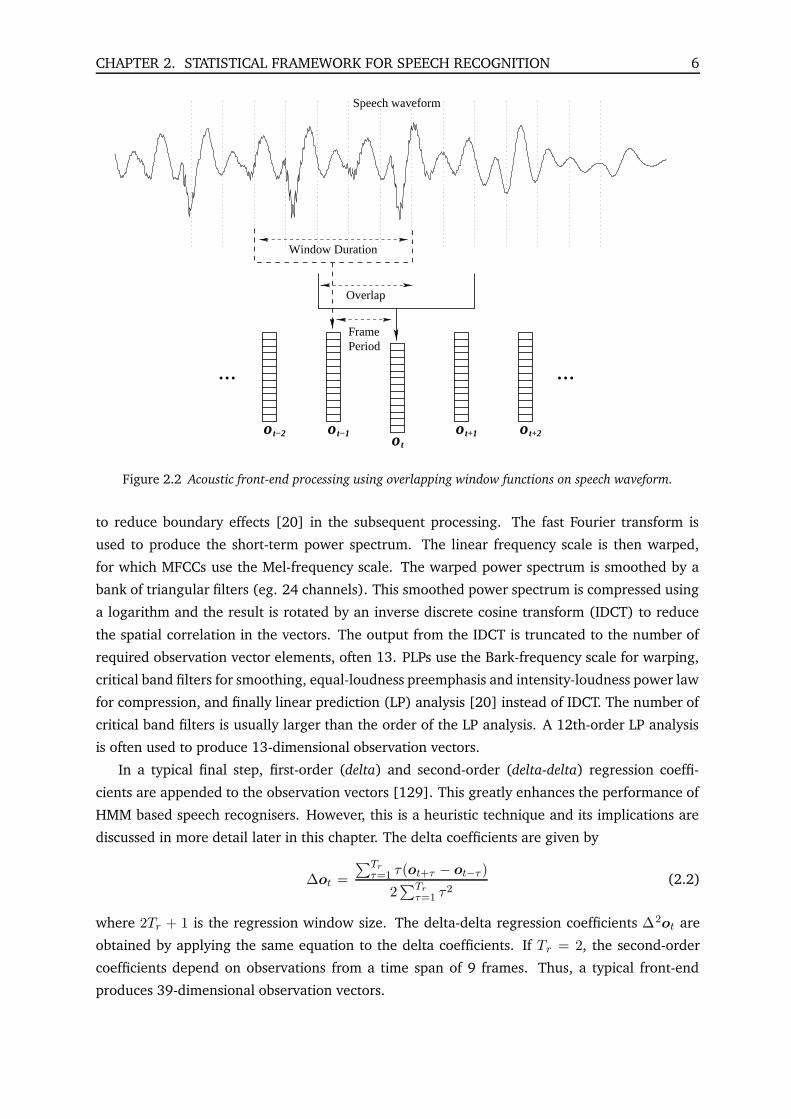
CHAPTER 2. STATISTICAL FRAMEWORK FOR SPEECH RECOGNITION 11
for 2 < t ≤ T , where cjn is the nth mixture weight associated with state j and bjn(ot) is the nth
Gaussian component evaluated at ot. The initial condition is given by
γjn(1) =1
p(O|θ(k))a1jcjnbjn(ot)βj(t) (2.20)
The re-estimation formulae for the parameters of the nth Gaussian mixture component associ-
ated with state j are given by
cjn =
∑Tt=1 γjn(t)
∑Tt=1 γj(t)
(2.21)
µjn =
∑Tt=1 γjn(t)ot
∑Tt=1 γjn(t)
(2.22)
Σjn =
∑Tt=1 γjn(t)(ot − µjn)(ot − µjn)
′
∑Tt=1 γjn(t)
(2.23)
The new set of model parameters, θ, is used as the current set of parameters, θ → θ(k+1),
in the following iteration. The iterations are continued until the change in the log-likelihood,
log(p(O|θ)) − log(p(O|θ(k))), falls below a set threshold. A disadvantage of the ML approach is
that the optimisation favours more complex models which produce higher log-likelihoods. The
models are easily over trained and the goodness of fit has to be evaluated by cross-validation.
The models that produce higher log-likelihoods for the training data do not necessarily perform
better for unseen data. This is due to the incorrect modelling assumptions described in Chapter
1. The ML estimates also tend to be inaccurate if there is not enough training data. The training
does not take any prior knowledge about the model parameters into account.
2.3.4 Bayesian Learning
In Bayesian learning [11], the parameters are also treated as random variables. The Bayesian
approach attempts to integrate over the possible settings of all uncertain quantities rather than
optimise them as ML learning in Equation 2.7. The quantity that results from integrating out
both the hidden variables and the parameters is called the marginal likelihood. For HMMs, this
can be written as
p(O) =
∫
p(θ)∑
∀Q
P (Q|θ)p(O|Q,θ) (2.24)
where p(θ) is a prior over the model parameters. The marginal likelihood is a key quantity
used to choose between different models in a Bayesian model selection task. The advantage
of Bayesian learning is that it does not favour more complex models and provides a means to
choose optimal models. However, evaluating the marginal likelihood for a HMM is not tractable
and approximate methods have to be used. Another challenge in Bayesian learning is the choice
of priors which is necessarily subjective [11].

CHAPTER 2. STATISTICAL FRAMEWORK FOR SPEECH RECOGNITION 12
Instead of full Bayesian learning, the maximum a-posteriori (MAP) [38] framework for HMMs
allows prior knowledge about the state conditional observation density parameters to be incor-
porated into parameter estimation. MAP training can be viewed as a parameter smoothing
scheme where the posterior likelihood is a combination of the prior and the ML estimates. In
case of insufficient data the posterior likelihood is close to the prior. In the limit the MAP es-
timates tend towards the ML estimates as the amount of training data increases. For example,
if insufficient data is available for ML estimation of context dependent models, the state con-
ditional observation density parameters from the context independent models may be used as
priors for context dependent models. Different modelling units are discussed in the following
section.
2.3.5 Discriminative Training
If the modelling assumptions were correct, the maximum likelihood criterion would be optimal
given infinite amount of data and an algorithm which finds the global maximum. However, it
has been found that discriminative training yields better performance than ML. Discriminative
optimisation criteria include maximum mutual information (MMI) [6], minimum classification
error rate (MCE) [65], frame discrimination [69] and minimum phone error rate [106] of which
MMI and MPE have been the most successful in speech recognition [49, 128]. In comparison
to ML training, the discriminative methods require recognition runs to be carried out during
training. This makes it much more demanding computationally. However, in this work only ML
training is considered.
2.4 Speech Recognition Using HMMs
The application of HMMs in speech recognition is presented in this section. First, the choice of
recognition units and model topologies is presented. Also, language modelling, recognition al-
gorithms as well as scoring and confidence measures are briefly reviewed. Finally, normalisation
and adaptation for HMM based speech recognition are presented.
2.4.1 Recognition Units
The HMMs may be used to provide the estimates of p(O|W ) in speech recognisers. For isolated
word recognition with sufficient training data it is possible to build a HMM for each word. How-
ever, for continuous speech tasks it is unlikely that there are enough training examples of each
word in the dictionary. HMMs representing some sub-word units have to be used. Linguistic
units such as phonemes or syllables may be used [100]. However, it has been found that au-
tomatically derived units perform better than units based on expert knowledge [5]. HMMs are
usually trained for each sub-word unit called a phone. The phone model set does not have to
represent every phoneme in the language and it often includes silence and short pause models
[129]. The chosen phone set depends on the availability of sufficient training data. The lexicon

CHAPTER 2. STATISTICAL FRAMEWORK FOR SPEECH RECOGNITION 13
or pronunciation dictionary is used to map word sequences to phone sequences. The HMMs
corresponding to the phone sequence may then be concatenated to form a composite model
representing words and sentences. This is also known as the beads-on-a-string procedure.
t−ih+n t−ih+ng f−ih+l s−ih+l
Figure 2.4 Example of single Gaussian triphones before and after state clustering.
When HMMs are trained for the set of basic phones, it is referred to as a monophone or
context independent system. There is, however, a considerable amount of variation between re-
alisations of the same phone depending on the preceding and following phones. This effect is
called co-articulation and is due to the inertia restricting any abrupt movement of the articu-
lators. Context dependent phone models acknowledge the influence of the surrounding phones
on the realisation. Commonly used context dependent phones are triphones which take the
preceding and following phones into account. Cross word triphones model contexts over word
boundaries and word internal triphones only within a word. Biphones are therefore used with
word internal triphones to allow start and end phones to be modelled. The number of states,
and model parameters, is significantly higher in a triphone system compared to a monophone
system. It is therefore unlikely that sufficient training data will be available for reliable parame-
ter estimation. The most common solution is to share some of the model parameters by tying the
state conditional observation densities among different models. The clustering of single mixture
Gaussian distributions is illustrated in Figure 2.4. An important question is how to determine
when states should share the same parameters.
A phonetic decision tree [130] is often used to produce the state clustering in triphone sys-
tems. Figure 2.5 shows an example of a decision tree where binary ‘yes/no’ questions are asked.
All instances of a phone are first pooled in the root node and the state clusters are split based on
contextual questions. The splitting will terminate in the final leaves or if the number of training
data examples per state falls below a set threshold. Expert knowledge may be incorporated into
the decision tree and every state is guaranteed to have a minimum amount of training data. A
disadvantage of decision tree clustering is that the splits maximise the likelihood of the training
data only locally [98].

CHAPTER 2. STATISTICAL FRAMEWORK FOR SPEECH RECOGNITION 14
Right/l/
Right/l/
No
Phone/ih/
NasalLeft
RightLiquid
Left Fricative
Model D Model E
Model C
Model BModel A
NoYes
Yes
Yes
Yes NoNo
Figure 2.5 Example of a phonetic decision tree for triphone models (from [130]).
2.4.2 Language Models
The language model provides the estimates of P (W ) in speech recognisers. Using the chain rule
this can be expressed as
P (W ) =
L∏
l=1
P (wl|wl−1, . . . , w1) (2.25)
In continuous speech recognition tasks, the vocabulary is too large to allow robust estimation of
P (W ). To reduce the number of parameters, different histories may be divided into equivalence
classes using a function h(wl−1, . . . , w1). The simplest, commonly used, equivalence classes are
defined by truncating the history to N − 1 words. These N -gram language models may be
expressed as
P (W ) =L∏
l=1
P (wl|wl−1, . . . , wl−N+1) (2.26)
Typical values are N = 2, 3, 4 which are called bi-, tri- or four-gram models respectively. The
ML estimation of the N -grams are obtained simply by counting relative frequencies from real,
often domain specific, text documents. For a vocabulary of V words there are still V N N -gram
probabilities. Some of the word sequences may be so absurd that zero probabilities may be
assigned, but given a finite training data, some valid word sequences may also be assigned a
zero probability. A number of smoothing schemes such as discounting, backing off and deleted
interpolation [70] have been proposed.
There is often a mismatch between the contribution of the acoustic model and the language
model in speech recognisers. This is due to different dynamic ranges of the discrete probability
mass function, P (W ), estimated from a finite set of text documents and the likelihood score,

CHAPTER 2. STATISTICAL FRAMEWORK FOR SPEECH RECOGNITION 15
p(O|W ), obtained from high dimensional observation densities. To compensate for this mis-
match many systems raise the language model probability to the power of a constant called
the grammar scale factor. The speech recognisers also tend to favour short words resulting in
many insertion errors. This is often compensated for by introducing an insertion penalty which
scales down the total score p(O|W )P (W ) depending on the number of hypothesised words in
the sequence. By taking these modifications into account in Equation 2.1, a practical speech
recogniser uses
W = arg maxW
(
log(p(O|W )
)+ α log
(P (W ) + βL
))
(2.27)
where α is the grammar scale factor, β is the insertion penalty and L is the total number of
words in the hypothesis. The parameters α and β are empirically set. The terms inside the
maximisation are often called the acoustic and language model scores. Logarithms are also taken
to deal with the high dynamic range and prevent underflow due to repeated multiplications of
values between zero and one.
2.4.3 Recognition Algorithms
An efficient recognition algorithm is required to solve Equation 2.27. An optimal decoder must
be able to search through all the word sequences to find the one yielding the maximum com-
bined score from the acoustic and language model. Direct implementation of this is not practical.
Instead the word sequence producing the maximum likelihood state sequence is searched for.
There is an efficient algorithm to find the maximum likelihood state sequence called the Viterbi
algorithm [125]. The Viterbi algorithm is based on a variable φj(t) which represents the max-
imum likelihood of observing vectors o1, . . . ,ot and being in state j at time t. This variable
differs from the forward variable in Section 2.3.3 by replacing the summation with a maximum
operator. The initial conditions are given by
φ1(1) = 1 (2.28)
φj(1) = a1jbj(o1) (2.29)
for 1 < j < Ns and the rest of the variables are given recursively by
φj(t) = maxi
(φi(t− 1)aij
)bj(ot) (2.30)
for 1 < j < Ns. The Viterbi algorithm results in the joint likelihood of the observation sequence,
O, and the most likely state sequence, Q, given the model. This is given by the variable in the
exit state at time T
φNs(T ) = p(O, Q|θ) = maxi
(φi(T )aiNs
)(2.31)
The most likely state sequence may be obtained by tracing back from the most likely final state.
It is straightforward to extend the Viterbi algorithm for continuous speech recognition. An
efficient implementation is called the token passing algorithm [131] where the current score and

CHAPTER 2. STATISTICAL FRAMEWORK FOR SPEECH RECOGNITION 16
a link to the previous word link record are propagated in tokens through the composite models.
A new word link record is generated every time instant by finding the token with the highest
score from the exit states of each composite word model. The language model score and the
insertion penalty are also stored to give the partial joint score. The word link record consists of
the partial score and the link to the previous word link record copied from the best exit token
along with the name of the word model where the token came from. Pruning may be used to
keep the number of active models from growing too large in large vocabulary continuous speech
recognition. However, excessively tight pruning may result in search errors. After the final
observation in the utterance has been processed the final word link record holds the total score
of the best hypothesis. The ML word sequence is found by following back word link records
using the links stored inside the records.
2.4.4 Scoring and Confidence
The performance of a speech recogniser is evaluated by comparing the hypothesised word se-
quence, W , to a reference transcription. These sequences are matched by performing an op-
timal string match using dynamic programming. Once the optimal alignment has been found,
the number of substitution errors, S, deletion errors, D, and insertion errors, I, are calculated.
Usually, the percentage word error rate (WER) is quoted. The WER is given by
WER = 100 ×(
1 −N −D − S − I
N
)
(2.32)
where N is the total number of words in the correct transcription [129].
When comparing the performance of different systems, it is useful to have a measure of
confidence in the relative difference in the WER. McNemar’s test [44] is used in this work to
yield the percentage probability, P (MINUUE|TUUE), where MINUUE is the minimum number
of unique utterance errors of two systems under consideration and TUUE is the total number of
unique errors. A confidence level is given as
Conf = 100 × [1 − P (MINUUE|TUUE)] (2.33)
and a statistically significant difference in two results may be taken at a 95% confidence level.
2.4.5 Normalisation and Adaptation
Characteristics of speech sounds vary substantially depending on the speaker and the acoustic
environment. Models trained on speaker specific data outperform models trained on speaker in-
dependent data. Normalisation attempts to represent all speech data in some canonical form
where the variance between speakers or environments does not lower the recognition per-
formance. For example vocal tract length normalisation [75, 124] for speaker normalisation,
and cepstral mean and variance normalisation [49] for environment normalisation are widely
adopted. Instead of normalising all speech data, the models may be adapted to represent the

CHAPTER 2. STATISTICAL FRAMEWORK FOR SPEECH RECOGNITION 17
characteristics of a new speaker or environment. The MAP [38] framework, discussed in Section
2.3.4, may be applied to speaker adaptation by using the speaker independent model parameters
as the priors which are gradually updated using the MAP rule towards parameters representing
the new speaker as more speaker dependent data comes available.
Maximum likelihood linear regression (MLLR) [77] is another model based adaptation scheme.
The adaptation of the mean vectors may be expressed as
µjn = Aµjn + b = Mξjn (2.34)
where ξjn is the augmented mean vector, [1 µjn]′, and M is the extended transform, [b′ A′]′.
The transform parameters are optimised using the EM algorithm with adaptation data from the
new speaker. The lth row vector ml of the extended transform matrix can be written as [78]
ml = k′lG
−1l (2.35)
where the matrix Gl and column vector kl are defined as follows
Gl =
Ns∑
j=1
M∑
n=1
1
σ2jnl
ξjnξ′jn
T∑
t=1
γjn(t) (2.36)
kl =
Ns∑
j=1
M∑
n=1
1
σ2jnl
T∑
t=1
γjn(t)otlξjn (2.37)
where σ2jnl is the lth diagonal element of the covariance matrix Σjn and otl is the lth element of
the current observation.
1
2 3
4 5 6 7
Figure 2.6 Example of a binary regression tree for MLLR speaker adaptation.
A single MLLR transform may be applied to all the models in the system in which case it
is called a global adaptation transform. Provided there are enough data the adaptation may
be improved by increasing the number of transforms. To define the number of transforms and
how to group the components into these transform classes, regression class trees [32] are often
used. A binary regression class tree is constructed to cluster together components that are
close in acoustic space. A simple example of such a tree is shown in Figure 2.6. The root
node corresponds to all the components pooled into one transform class; i.e., a global MLLR
transform. The splitting of each node continues until the number of components assigned to a

CHAPTER 2. STATISTICAL FRAMEWORK FOR SPEECH RECOGNITION 18
specific class falls below a set threshold. In the figure, nodes 5, 6 and 7 do not have sufficient
data and the components are pooled back to the node above. The final number of transform
classes is three in this example.
2.5 Covariance and Precision Modelling
As discussed in Section 2.3.1, the form of the covariance matrix for each Gaussian component
is important in HMM based speech recognition. Traditionally, a simple choice between full and
diagonal covariance matrices has been made. For p-dimensional observations, a full covariance
matrix has p(p + 1)/2 parameters and a diagonal covariance matrix has p parameters. The
number of Gaussian components in LVCSR tasks is tens of thousands and the dimensionality
of the observations is high, often p = 39. The robust estimation of model parameters in such a
large system is hard given a limited amount of training data. Hence diagonal covariance matrices
are a popular choice. Recently a number of schemes to interpolate between the diagonal and
full covariance matrix assumptions have been proposed. The first set of such schemes models
the covariance matrices directly whereas the second models the inverse covariance (precision)
matrices.
Assuming there are J Gaussian components in the HMM system, the jth Gaussian evaluated
at an observation ot may be written as
p(ot|j) = (2π)−p
2 |Σj |− 1
2 e−12(ot−µj)
′Σ
−1j (ot−µj) (2.38)
where the constant including the determinant of the covariance matrix may be precomputed for
each component. The quadratic term in the exponent is the most expensive operation computa-
tionally. For diagonal covariance matrices O(p) multiplications and for full covariance matrices
O(p2) multiplications have to be computed. It should be noted that the inverse covariance ma-
trices may be stored to avoid inverting the matrices during the likelihood calculation when full
covariance matrices are used.
2.5.1 Covariance Matrix Modelling
Factor analysis is a statistical method for modelling the covariance structure of high dimensional
data with a small number of hidden variables [63]. The use of factor analysis for covariance
modelling in speech recognition has been investigated [122]. In factor analysis the covariance
matrix assumes the following form
Σj = CjC′j + Σ
(o)j =
k∑
i=1
cjic′ji +
p∑
i=1
σ(o)2ji eie
′i (2.39)
where Σ(o)j = diag(σ
(o)2j1 , . . . , σ
(o)2jp ) is a component specific diagonal covariance matrix in the p-
dimensional observation space, C j = [cj1, . . . , cjk] is a component specific p by k factor loading
matrix and ei is the ith p-dimensional unit vector. There are fewer model parameters compared

CHAPTER 2. STATISTICAL FRAMEWORK FOR SPEECH RECOGNITION 19
to full covariance matrices if the number of factors, k, satisfies k < (p − 1)/2. However, this
model has a large number of free parameters due to the component specific loading matrices
and some sharing schemes have been investigated [48]. The covariance matrix for this shared
factor analysis (SFA) may be expressed as
Σj = CsC′s + Σ
(o)j =
k∑
i=1
csic′si +
p∑
i=1
σ(o)2ji eie
′i (2.40)
where the index s defines how the loading matrices are shared among a number of Gaussian
components. For a global loading matrix the index may be omitted. An alternative sharing
scheme called independent factor analysis (IFA) [2] has been proposed in the machine learning
literature. The covariance matrix for IFA assumes the following form
Σj = CsΣ(x)j C ′
s + Σ(o)s =
k∑
i=1
σ(x)2ji csic
′si +
p∑
i=1
σ(o)2si eie
′i (2.41)
where Σ(x)j = diag(σ
(x)2j1 , . . . , σ
(x)2jp ) is a component specific diagonal covariance matrix in the
k-dimensional subspace. In the IFA, both the loading matrices and p-dimensional covariance
matrices are shared among a number of Gaussian components. For all the covariance models
based on factor analysis, the covariance matrices, Σ(o), are important to guarantee the com-
ponent covariance matrices, Σj , being non-singular since the terms, CC ′ and CΣ(x)C ′, are at
most rank-k matrices.
Alternative covariance modelling schemes operate in the full p-dimensional observation space
using linear transforms. In these schemes each component has a diagonal component specific
covariance matrix. A number of p by p linear transforms, similar to the loading matrices in
factor analysis, are applied to yield full covariance matrices. It should be noted that since the
transforms are p by p matrices, there is no need for additional observation covariance matrices.
The covariance matrix for this semi-tied full covariance matrix (STC) [34] may be expressed as
follows
Σj = CsΣ(d)j C ′
s =
p∑
i=1
σ(d)2ji csic
′si (2.42)
where Σ(d)j = diag(σ
(d)2j1 , . . . , σ
(d)2jp ) is a p-dimensional component specific diagonal covariance
matrix and Cs = [cs1, . . . , csp] is a semi-tied transform matrix shared among a number of Gaus-
sian components. If the transform matrices are shared globally, the model reduces to the max-
imum likelihood linear transform (MLLT) [47] scheme. The STC scheme is closely related to
heteroscedastic linear discriminant analysis (HLDA) based schemes [35, 72]. A common ad-
vantage of these schemes compared to factor analysis based schemes is the efficient likelihood
calculation. Since HLDA and STC may be viewed as feature space transforms, the likelihood
calculations operate on diagonal covariance matrices after applying the transforms to the obser-
vation vectors. HLDA has also been successfully used in state of the art systems [49].
The choice of the sharing scheme for SFA, IFA, STC and HLDA schemes is important due to
the total number of free parameters in the system. For STC often a single transform is used

CHAPTER 2. STATISTICAL FRAMEWORK FOR SPEECH RECOGNITION 20
[34, 47]. However, these systems are very flexible since tying the transforms over a number
of Gaussian components can be used to produce various combinations of transform classes.
The tying may be based on regression class tree clustering as described in Section 2.4.5. The
regression class tree attempts to cluster together components that are close in acoustic space.
HLDA systems have additional degrees of freedom due to the number of retained dimensions
(state vector dimensionality). Automatic complexity control for HLDA systems is under active
research [80, 81]. For SFA the loading matrices may be specific to each HMM state since the
increase in the number of free parameters is not very significant if k p. Also, various tying
schemes are possible for the IFA and SFA. However, the number of possible configurations is vast
and automatic schemes should be employed.
2.5.2 Precision Matrix Modelling
Direct modelling of the inverse covariance (precision) matrices has recently been investigated
[4, 99]. Having the component Equation 2.38 to yield valid likelihoods, it is required that the
covariance matrices be positive definite; that is, x′Σjx ≥ 0 for all x ∈ R
p. In cases of the
covariance matrix modelling schemes above, this means that all diagonal elements of Σ(o)j , Σ
(x)j
and Σ(d)j have to be positive. If instead the MLLT scheme is generalised as follows
Σ−1j = AΛjA
′ =
k∑
i=1
λjiaia′i (2.43)
where A = [a1, . . . ,ak] is a global p by k matrix, Λj = diag(λj1, . . . , λjk) is a diagonal compo-
nent specific matrix of expansion coefficients and k > p, the coefficients are not required to be
positive. The only restriction on the coefficients λji is that the resulting precision matrix must
be positive definite. This scheme is called the extended MLLT (EMLLT) [99]. Using the sum
representation on the right hand side in Equation 2.43, the precision matrix may be viewed as
a linear combination of a collection of k rank-1 matrices aia′i. By using particular bases, the
EMLLT scheme may be viewed as interpolating between MLLT when k = p and full covariance
model when k = p(p+ 1)/2.
Recently a generalisation of EMLLT called subspace model for precision matrices and means
(SPAM) has been proposed [4]. Instead of using rank-1 matrices as the basis, a collection of k
shared p by p basis matrices Si are used to model the precision matrix as follows
Σ−1j =
k∑
i=1
λjiSi (2.44)
where 1 ≤ k ≤ p(p + 1)/2. The basis matrices are not required to be positive definite. In
common with EMLLT, the only restriction on the coefficients λji and basis matrices Si is that the
resulting precision matrix must be positive definite. In the SPAM scheme also the mean vectors
are assumed to lie in a subspace of Rp spanned by k basis vectors.

CHAPTER 2. STATISTICAL FRAMEWORK FOR SPEECH RECOGNITION 21
Both EMLLT and SPAM systems have been shown to outperform global STC (MLLT) systems.
The SPAM was found to outperform EMLLT systems with similar complexity in [4]. The perfor-
mance of EMLLT systems using multiple subspaces instead of the one defined by a set of global
rank-1 matrices aia′i was investigated in [23]. It was found that multiple subspace scheme
outperforms the standard EMLLT and a data driven clustering based on matrix norms outper-
forms phonetic and sub-phonetic clustering schemes. Regression tree clustering may also be
used for the clustering.
2.6 Segment Models
Segment models [71, 102] have been proposed to address the state conditional independence
assumption made in the HMM. Instead of generating conditionally independent observation
vectors, the discrete states in a segment model generate a sequence of observations length l.
The joint likelihood of an observation sequence given a discrete state q may be written as
p(o1:l, l|q) = p(o1:l|l, q)P (l|q) = bq,l(o1:l)P (l|q) (2.45)
where P (l|q) is a duration model and bq,l(o1:l) is an output probability density function for
variable length observation sequences. If the output density function assumes the observations
independent and identically distributed, the segment model reduces to a HMM with an explicit
duration model. However, the goal of the segment models is to provide an explicit model for
the temporal correlation between observations in a segment and more elaborate output density
functions have been considered.
General inference and training schemes for segment models have been described in [102].
Viterbi decoding was generalised for segment models. Due to the underlying duration model, the
Viterbi algorithm has to consider all the possible segmentations of the observation sequence. For
an utterance of length T there are O(2T ) segmentations that must be considered in an optimal
search. A number of schemes to reduce the search space have been introduced [102]. Also, a
generalised forward-backward algorithm was presented. Due to the increased complexity, the
most likely state sequence estimation has often been used [24, 102]. Segmental HMMs [37, 56,
57, 58, 59, 60] have also been proposed to overcome the inter-frame correlation problem with
some success on monophone and biphone classification tasks using TIMIT corpus. However,
segment models and segmental HMMs scale poorly to larger tasks.
2.6.1 Stochastic Segment Model
A linear dynamical system (LDS) has been used as a segment conditional output density function
[24, 101]. This model is called the stochastic segment model (SSM). A LDS is described by the
following two equations
xt = Axt−1 + w (2.46)
ot = Cxt + v (2.47)

CHAPTER 2. STATISTICAL FRAMEWORK FOR SPEECH RECOGNITION 22
where xt is a k-dimensional state vector. The matrices A and C are called the state evolu-
tion matrix and the observation matrix, respectively. The noise vectors w ∼ N (µ(x),Σ(x))
and v ∼ N (µ(o),Σ(o)) are assumed to be independent and called state evolution noise and
observation noise, respectively. The initial state is also assumed to be Gaussian distributed,
x1 ∼ N (µ(i),Σ(i)).
In the original work on SSMs [24], the dimensionality of the state vectors was assumed
to be k = p, the state evolution noise mean vector equal to zero µ(x) = 0, observation noise
covariance matrix Σ(o) shared globally and the observation matrix equal to the identity matrix
C = I . Due to variable speaking rates, either deterministic or dynamic distribution mappings
were used for each segment. The deterministic mapping assumed a number of regions within
segments having fixed parameters. This corresponds to a segment model with multiple discrete
states per phone in the general notation above. The dynamic distribution mapping assumed a
single set of parameters per phone but a linear time warping was used to normalise segment
durations before the model was applied. Some gains compared to HMMs in phone classification
task using TIMIT [73] corpus were reported. The application of LDSs for speech recognition has
recently been addressed elsewhere [29, 30].
Most of the other segment models presented in the literature may be regarded as a special
case of the SSM. A good review of these approaches has been provided [102]. A number of
disadvantages in the segment models may be identified. Firstly, the increased number of free
parameters in the models may result in poor estimates due to limited amount of training data.
Secondly, the segments are assumed to be independent. It is believed that due to strong co-
articulation in speech, this assumption is not valid. Thirdly, most of the segment conditional
output densities considered can only represent unimodal distributions although the observation
vector distributions are often more complex due to speaker and environment variability.
2.6.2 Hidden Dynamic Models
Recently, similar models to SSMs called hidden dynamic models (HDMs) have been proposed
[22, 84, 105, 111, 133]. HDM is based on a non-linear state evolution process as opposed to
the linear state evolution in the LDS above. This non-linear state evolution is approximated
by the first two terms of its Taylor series expansion. The observation process in HDMs is often
implemented by a global multi-layer perceptron. However, factor analysis based observation
process has been proposed [84] as in the standard LDS above but the parameters were allowed
to switch between frames. This approach effectively can model non-Gaussian distributions the
same way as the mixture of LDSs [113]. Despite the linearisation in state space, the inference
algorithms for the HDM are intractable. A number of approximate methods have been pro-
posed [76, 82, 83, 85, 123]. Some gains compared to HMMs were reported in N -best rescoring
experiments using various subsets of the Switchboard [45] corpus.

CHAPTER 2. STATISTICAL FRAMEWORK FOR SPEECH RECOGNITION 23
2.7 Summary
The statistical framework for speech recognition has been described in this chapter. First, the
standard front-ends were briefly reviewed. The hidden Markov model was then described as a
generative model for multivariate observation vectors. Parameter optimisation schemes based
on the maximum likelihood estimation, Bayesian learning and discriminative training were pre-
sented. The application of HMMs to acoustic modelling was described. Language models,
recognition algorithms, scoring and adaptation for HMM based speech recognition were also
presented. The form of the covariance matrix is important in HMMs. A number of covari-
ance and precision matrix modelling techniques were described. Finally, segment models were
presented as alternative acoustic models to HMMs. Segment models have been developed to
address the shortcomings in HMMs described in Chapter 1.

3
Generalised Linear Gaussian Models
This chapter presents generalised linear Gaussian models in a generative model framework.
First, standard state space model terminology is reviewed. Then, dynamic Bayesian networks
are reviewed as a method to illustrate conditional independence assumptions made in the model.
Linear Gaussian models and a generalisation to include Gaussian mixture models are also dis-
cussed. Classification of linear Gaussian models according to different state evolution and obser-
vation process assumptions is presented followed by a discussion about standard models using
factor analysis and linear dynamical system as examples.
3.1 State Space Models
State space models are generally based on a k-dimensional state vector, xt, and a p-dimensional
observation vector, ot, which satisfy the following generative model
xt+1 = f(x1, . . . ,xt,wt)
ot = g(xt,vt)(3.1)
where the functions f(·) and g(·) define the state evolution and observation processes, respec-
tively. The random vectors wt and vt are called the state evolution noise and observation noise.
Although the models described above may exhibit any linear or non-linear functions, the models
presented in this work are restricted to linear ones. By the strict definition of linear Gaussian
models, the noise sources wt and vt are Gaussian distributed with the following densities
wt ∼ N (µ(x)t ,Σ
(x)t ) (3.2)
vt ∼ N (µ(o)t ,Σ
(o)t ) (3.3)
However, in many problems the observation vectors do not have unimodal distributions. In
speech signals, for example, the feature vector distributions have several modes due to speaker
and environment variability. In this work the unimodal assumption is relaxed by including
mixture models – hence the name generalised linear Gaussian models.
24

CHAPTER 3. GENERALISED LINEAR GAUSSIAN MODELS 25
The state evolution process may be viewed as some underlying phenomenon which may be
inherent for the signal being modelled. Alternatively, it may only be viewed as a compact repre-
sentation of the correlation in the high dimensional observation vectors. For example, in speech
recognition the state vector may be viewed as representing positions of the articulators and the
state evolution process, f(·), describes their movement in time. Although the above generic
model fits into this interpretation, the linear Gaussian models are a crude approximation since
the movement of articulators is non-linear [14]. Due to this non-linear nature, the articulatory
interpretation is not often stressed in this work.
The observation equation, g(·), describes the function mapping the current state vector, xt,
mixed with the observation noise, vt, onto the current observation, ot, which is usually higher in
dimensionality; that is, p > k. For example, in speech recognition the observation process may
be viewed as mapping the positions of the articulatory organs onto the acoustic representation
where the observation noise, vt, represents all the noise induced by the environment and the
recording equipment. As in the case of the state evolution process, this interpretation is only
valid for non-linear models [14]. In this work, the observation process is an important part of
the correlation model for the high dimensional observation vectors.
3.2 Bayesian Networks
In this work, Bayesian networks [39, 96] are used to illustrate the statistical independence as-
sumptions between different random variables in probabilistic models. Bayesian networks are
directed acyclic graphs, also known as graphical models. The notation used in this work is
adopted from [93] where round nodes were used to denote continuous and square nodes dis-
crete random variables. The observable variables are shaded. Missing arrows between variables
represent conditional independence assumptions.
z
x
o
z
x
o
t+1qqt
1 2 3
Figure 3.1 Examples of Bayesian networks representing different assumptions on conditional independence.
1) No independence assumptions between continuous random variables z, x and o (shading denotes observ-
able), 2) random variable o is conditionally independent of z given x, 3) discrete random variable qt+1 is
conditionally independent of all its predecessors given qt (discrete Markov chain).

CHAPTER 3. GENERALISED LINEAR GAUSSIAN MODELS 26
As an example, three continuous random variables z, x and o are considered. The variable o
is observed and the others are hidden (latent). The joint likelihood can be factored as a product
of conditional likelihoods as follows
p(z,x,o) = p(z)p(x|z)p(o|x, z) (3.4)
This factorisation is perfectly valid in every case. If no assumptions of conditional indepen-
dence can be made, the corresponding Bayesian network must be illustrated as the first network
in Figure 3.1. There are two arrows pointing to the node representing o, since in the above
factorisation o depends on both z and x.
If the random variable o is assumed to be conditionally independent of z given x the joint
likelihood can be rewritten as follows
p(z,x,o) = p(z)p(x|z)p(o|x) (3.5)
The corresponding Bayesian network is depicted as the second graph in Figure 3.1. Thus, the
arrow between the nodes representing z and o can be deleted.
As another example, an ordered set of discrete random variables, Q = q1, . . . , qT , is consid-
ered. The joint likelihood of the variables up to time instant t+1 can be written using conditional
likelihoods as follows
P (q1, . . . , qt+1) = P (q1)P (q2|q1)P (q3|q1, q2) . . . P (qt+1|q1, . . . , qt) (3.6)
Often a simplification is achieved by using a Markov assumption, which says that the likeli-
hood of the variable qt+1 is conditionally independent of all other preceding variables, given the
immediate predecessor qt; that is,
P (qt+1|q1, . . . , qt) = P (qt+1|qt) (3.7)
This is often called a discrete Markov chain and is illustrated as the third graph in Figure 3.1.
ot ot+1
t+1qqt
Figure 3.2 Dynamic Bayesian network representing a hidden Markov model.
Dynamic Bayesian networks (DBN) [135] may be used to illustrate the conditional indepen-
dence assumption made in a HMM. A DBN representing a HMM is shown in Figure 3.2. It can
be seen that the new observation, ot+1, is conditionally independent of the previous discrete
states and observations given the new state, qt+1. Furthermore, the new discrete state, qt+1, is
conditionally independent of the previous discrete states, given the immediate predecessor, qt;
that is, Markov assumption.

CHAPTER 3. GENERALISED LINEAR GAUSSIAN MODELS 27
3.3 State Evolution Process
The number of possible state evolution processes in linear Gaussian models is restricted. Several
static models may also be classified as linear Gaussian models [119]. However, only dynamic
state evolution processes are considered in this work. In this section, a piece-wise constant and
a first-order linear Gauss-Markov state evolution process are described. The continuous state
trajectories that may be represented by these models are discussed.
3.3.1 Piece-Wise Constant State Evolution
The first dynamic state evolution process is based on a hidden Markov model. As described in
Chapter 2, a HMM is defined by the state transition probabilities, aij , and state conditional ob-
servation densities, bj(ot). When a HMM is used as the state evolution process the observation
vectors, ot, are replaced by the state vectors, xt. The discrete HMM state controls which contin-
uous state density generates these state vectors. The continuous state statistics remain constant
until the discrete state switches – hence the name piece-wise constant state evolution.
The piece-wise constant state evolution process may be represented by the following gener-
ative model1
qt ∼ P (qt|qt−1)
xt = wqt , wj ∼∑
n c(x)jn N (µ
(x)jn ,Σ
(x)jn )
(3.8)
This state evolution process is illustrated by the state vector element trajectory on the left hand
side in Figure 3.3. Three discrete states with different discrete state conditional continuous state
vector densities are shown. It should be noted that the conditional independence assumption
of standard HMMs is present in any linear Gaussian model based on piece-wise constant state
evolution process, since the observation process depends only on the current state vector.
t
x1
t
x1
Figure 3.3 Trajectories of a state vector element illustrating different dynamic state evolution processes. The
piece-wise constant state evolution on the left hand side is based on a HMM. The linear continuous state
evolution on the right hand side is based on a first-order Gauss-Markov random process.
1The ∼ symbol in qt ∼ P (qt|qt−1) is used to represent a discrete Markov chain. Normally it means that the
variable on the left hand side is distributed according to the probability density function on the right hand side as in
x ∼ N (µ,Σ).

CHAPTER 3. GENERALISED LINEAR GAUSSIAN MODELS 28
3.3.2 Linear Continuous State Evolution
The second dynamic state evolution process is a linear first-order Gauss-Markov random process.
A Markov assumption is made to the general state evolution process in Equation 3.1 so that the
current state vector xt is conditionally independent of the previous state vectors, given the
immediately preceding one, xt−1. The new state vector is generated by a linear state evolution
process from the current state vector as follows
xt+1 = Axt + w, w ∼∑
n
c(x)n N (µ(x)n ,Σ(x)
n ) (3.9)
where A is a k by k state evolution matrix2 and w is the state evolution noise which usually
is a single Gaussian. Since the initial state vector, x1, is assumed to be a Gaussian with mean
vector µ(i) and covariance matrix Σ(i), all the subsequent state vectors are Gaussian distributed
as follows
p(xt|xt−1) = N (xt;Axt−1 + µ(x),Σ(x)) (3.10)
Furthermore, the state evolution noise is often assumed to be zero mean and spatially uncor-
related; that is, Σ(x) is diagonal. With a Gaussian mixture model a zero mean cannot be used.
Using diagonal covariance matrices reduces the number of model parameters and allows the
correlations to be modelled by the state evolution matrix.
Since the state evolution process encodes the temporal correlation in a linear Gaussian
model, it is interesting to see the kind of continuous state vector trajectories it can represent.
This requires more analysis compared to the piece-wise linear state evolution process described
above. The mean vector, µt, evolves according to a first-order ordinary difference equation with
constant coefficients
µt = Aµt−1 + µ(x) (3.11)
The homogeneous equation, µt − Aµt−1 = 0, has a solution µ(h)t = UΛ
t−1c [127] where U
is a matrix of eigenvectors of the state evolution matrix, A, the diagonal matrix, Λ, has the
eigenvalues of A as its elements, and c is a constant vector. A constant, µ(p)t = (I − A)−1µ(x),
may also be shown to be a particular solution to this difference equation. The general solution is
the sum of these two solutions. The constant vector c may be solved using the initial condition
µ1 = µ(i). Thus, the solution of the differential equation is
µt = At−1µ(i) + (I − At−1)(I − A)−1µ(x) (3.12)
The stability of this solution depends on the eigenvalues of the state evolution matrix. For
multiplying an arbitrary vector y repeatedly by the matrix A, the following limit may be derived
[127]
limt→∞
At−1y = λt−11 b1u1 (3.13)
2The discrete state transition probabilities aij are often represented as a state transition matrix A in speech
recognition literature. However, in this work A is used to represent the continuous state evolution matrix. Also, it
should not be confused with the MLLR and EMLLT transforms in Chapter 2.
CHAPTER 3. GENERALISED LINEAR GAUSSIAN MODELS 29
where b1 is a constant and, λ1 and u1 are the eigenvalue with the largest absolute value and
the corresponding eigenvector of A, respectively. Therefore, if |λ1| is greater than one, the state
vector grows exponentially in the direction of u1. If |λ1| is less than one, the state mean vector
converges towards the following limit
limt→∞
µt = (I − A)−1µ(x) (3.14)
Provided the largest eigenvalue of the state evolution matrix is less than one, the state evolution
process is stable. Thus, the individual state vector element trajectories for a stable linear first-
order Gauss-Markov state evolution process are damped oscillations buried in the observation
noise. One such trajectory is shown on the right hand side in Figure 3.3. The covariance matrix
of the state evolution process evolves through time as follows
Σt = AΣt−1A′ + Σ
(x) (3.15)
with initial condition Σ1 = Σ(i). The state evolution matrix may be enforced to be stable in the
parameter estimation [29]. However, the stability may not be an issue as long as the sequences
are short. Later in this work, the switching process guarantees short sequences.
3.4 Observation Process
Two different observation processes are presented in this section. Both processes handle dimen-
sion changes. Thus lower dimensional state spaces may be used; that is, k < p. The first process
is closely related to factor analysis and the second to linear discriminant analysis.
3.4.1 Factor Analysis
The first observation process is called factor analysis (FA) [120] since in a static case the model
reduces to a standard FA model with explicit factor mean and variance elements. The factor
analysis observation process can be represented as
ot = Ctxt + vt, vt ∼ N (µ(o)t ,Σ
(o)t ) (3.16)
where C t is a p by k observation matrix and vt is a p-dimensional observation noise. The
observation noise is independent of the state vector, xt, and its covariance matrix is assumed
to be diagonal. This is an important modelling assumption as the observation matrix is used
to represent the spatial correlation in the data. In the case of static data modelling, the time
indexes in the observation equation may be omitted. Due to the Gaussian observation noise, the
conditional likelihood of the observation vector given the state vector is given by the following
Gaussian
p(ot|xt) = N (ot;Ctxt + µ(o)t ,Σ
(o)t ) (3.17)

CHAPTER 3. GENERALISED LINEAR GAUSSIAN MODELS 30
xt
xt
ot
vt
Ct
Figure 3.4 An example illustrating factor analysis. The lower dimensional state vectors, xt, are stretched
and rotated by the observation matrix, Ct, in the observation space. This is convolved with the observation
noise distribution to produce the final distribution.
If the state vector is Gaussian distributed, the joint likelihood of the observation and state vector
is also a Gaussian.
The traditional factor analysis model assumes the state vectors are generated by a standard
normal distribution; that is, N (0, I). The factor analysis and different mixture assumptions are
described in more detail in Section 3.5.2. Factor analysis is illustrated in Figure 3.4. The samples
of the lower dimensional state vectors, xt, are first stretched and rotated by the observation ma-
trix, C t, in the observation space. This new distribution is then convolved with the observation
noise distribution which yields the final distribution.
3.4.2 Linear Discriminant Analysis
The second type of observation process is called linear discriminant analysis (LDA) [63] because
in the static case, the model reduces to a standard LDA. The meaningful dimensions are mod-
elled by a state vector, xt, and the “nuisance” dimensions are modelled by a single Gaussian
distributed observation noise as follows
ot = C
[
xt
v
]
, v ∼ N (µ(o),Σ(o)) (3.18)
where C is a global p by p matrix and v is a global (p− k)-dimensional noise vector. By defining
B = C−1 (3.19)

CHAPTER 3. GENERALISED LINEAR GAUSSIAN MODELS 31
the state vector is given by a deterministic linear projection
xt = B[p−k]ot (3.20)
where B[p−k] denotes a matrix consisting of the p−k top rows of matrix B. LDA may be viewed
as a projection scheme where the state vectors lie in the useful space and the noise spans the
nuisance dimensions. If the aim is to classify a set of observation vectors, the LDA projection
B may be optimised to maximise the between class variance and minimise the within class
variance. The standard LDA assumes within class covariance matrices to be same (global). An
extension to LDA called heteroscedastic LDA (HLDA) [72] relaxes this assumption. In the case
of piece-wise constant state evolution, the classes may be the different Gaussian components in
the system. HLDA and a number of other extensions have been applied to HMM based speech
recognition [35].
x
2
1
x
Figure 3.5 An example illustrating linear discriminant analysis. The black equal probability contours repre-
sent two classes which are not separable in the original space. LDA finds a projection down to one dimensional
space, x1, with maximum between class and minimum within class distance.
Linear discriminant analysis is illustrated in Figure 3.5. The black equal probability contours
represent covariance matrices of two classes, which are not easy to separate in the original
two dimensional space. LDA finds a projection that minimises the within class distance and
maximises the between class distance. The two classes may be easily separated in the new
1-dimensional space along the x1 axis, whereas the x2 axis represents the nuisance dimension.

CHAPTER 3. GENERALISED LINEAR GAUSSIAN MODELS 32
3.5 Standard Linear Gaussian Models
Different models combining the state and observation processes presented in the previous sec-
tions are reviewed in this section3. First, static models are presented using a factor analysis as
an example. Second, dynamic models with relations to the static models are reviewed. A linear
dynamical system is used as an example.
3.5.1 Static Models
Figure 3.6 depicts models based on static state evolution process. At the top of the diagram
is a single static multivariate Gaussian as the root for all the subsequent models. A mixture
of Gaussians can be regarded as a vector quantisation with the Gaussian mean vectors as the
cluster centres. Vector quantisation is often used in the initialisation of, for example, HMM
parameters [129]. Instead of using only one code-book to assign a vector into a single cluster,
cooperative vector quantisation [132] or factorial mixture of Gaussians uses several independent
code-books in a distributed manner. All of these three models correspond to a state space model
with identity matrix as the observation matrix and zero observation noise.
Gaussian
Factor AnalysisIndependent
Mixtured FA(MFA and SFA)
Factor Analysis
Factorial Mixtureof Gaussians
(CVQ)
Mixture ofGaussians (VQ) Analysis
Linear Discriminant
Factor Analysis=FALinear Discriminant Analysis=LDAMixture=MIXDistributed Representation=DIST
VQ = Vector Quantisation=CVQ Cooperative VQ
SFA = Shared Factor Analysis=MFA Mixture of Factor Analysers
MIX
DISTDISTMIX
FA
FA LDA
Figure 3.6 Diagram of static linear Gaussian models. The arrows represent additional properties to the
model they are attached to.
Factor analysis [46, 63, 120] is based on a static multivariate Gaussian state process and a
factor analysis observation process. In standard factor analysis the state vectors are assumed to
be distributed according to a standard normal distribution, N (0, I). Independent factor analysis
[2], mixture of factor analysers [40] and shared factor analysis [48] are based on the factor
analysis model with different mixture assumptions. These models are discussed in the example
below. Linear discriminant analysis [63] is another static data modelling scheme with linear
discriminant analysis observation process.
3These diagrams do not illustrate all the possible forms of linear Gaussian models. For example, several combina-
tions using LDA observation process have not been presented for brevity.

CHAPTER 3. GENERALISED LINEAR GAUSSIAN MODELS 33
3.5.2 Example: Factor Analysis
Factor analysis is a statistical method for modelling the covariance structure of high dimensional
data using a small number of latent (hidden) variables [63]. It is often used to model the data
instead of a Gaussian distribution with full covariance matrix. Factor analysis can be described
by the following generative model
x ∼ N (0, I)
o = Cx + v, v ∼ N (µ(o),Σ(o))(3.21)
where x is a collection of k factors (k-dimensional state vector) and o is a p-dimensional ob-
servation vector. The covariance structure is captured by the factor loading matrix (observation
matrix), C, which represents the linear transformation relationship between the state vector
and the observation vector. The mean of the observations is determined by the error (observa-
tion noise) modelled as a single Gaussian with mean vector µ(o) and diagonal covariance matrix
Σ(o). The observation process can be expressed as a conditional likelihood given by
p(o|x) = N (o;Cx + µ(o),Σ(o)) (3.22)
This may be illustrated by the simple Bayesian network in Figure 3.7. Also, the observation
likelihood is a Gaussian with mean vector µ(o) and covariance matrix CC ′ + Σ(o).
x
o
Figure 3.7 Bayesian network representing a standard factor analysis model.
The number of model parameters in a factor analysis model is η = p(k + 2). It should be
noted that any non-zero state space mean vector, µ(x), can be absorbed by the observation mean
vector by adding Cµ(x) into µ(o). Furthermore, any non-identity state space covariance matrix,
Σ(x), can be transformed into an identity matrix using eigen decomposition, Σ(x) = UΛU ′. The
matrix U consists of the eigenvectors of Σ(x) and Λ is a diagonal matrix with the eigenvalues
of Σ(x) on the main diagonal. The eigen decomposition always exists and is real valued, since a
valid covariance matrix is symmetric and positive definite. The transformation can be subsumed
into the observation matrix by multiplying C from the right by UΛ1/2. It is also essential that
the observation noise covariance matrix be diagonal. Otherwise, the sample statistics of the
data can be set as the observation noise and the loading matrix equal to zero. As the number of
model parameters in a Gaussian with full covariance matrix is η = p(p+ 3)/2, a reduction in the
number of model parameters using factor analysis model can be achieved by choosing the state
space dimensionality according to k < (p− 1)/2.

CHAPTER 3. GENERALISED LINEAR GAUSSIAN MODELS 34
The expectation maximisation (EM) algorithm [21] may be used to obtain maximum like-
lihood estimates for the parameters of a factor analyser [120]. Given a set of N observations,
O = o1, . . . ,oN, the inference requires simply estimating the state posterior statistics as fol-
lows
xn = Ex|on,θ(k) = K(on − µ(o)) (3.23)
Rn = Exx′|on,θ(k) = I − KC + xnx
′n (3.24)
where K = C ′(CC ′ + Σ(o))−1 and θ(k) is the set of model parameters in the kth iteration. It
should be noted that using the result in Appendix B, the inverse of the p by p matrix (CC ′ +
Σ(o))−1 may be evaluated efficiently as follows
(CC ′ + Σ(o))−1 = Σ
(o)−1 −Σ(o)−1C(C ′
Σ(o)−1C + I)C ′
Σ(o)−1 (3.25)
where the inverse of the diagonal covariance matrix Σ(o) is trivial to compute and only an inverse
of a k by k matrix (C ′Σ
(o)−1C+I) has to be evaluated. This is considerably faster than inverting
a full p by p matrix if k p.
A new set of model parameters θ may be obtained as follows
[
C µ(o)]
=( N∑
n=1
[
onx′n on
] )( N∑
n=1
[
Rn xn
x′n 1
])−1
(3.26)
Σ(o)
=1
N
N∑
n=1
diag(
ono′n −
[
C µ(o)] [
onx′n on
]′ )
(3.27)
These parameters are set as the new parameters θ → θ(k+1) for the following iteration until no
significant change in the log-likelihood is observed.
Factor analysis has been extended to employ Gaussian mixture models for the factors in IFA
[2] and the observation noise in SFA [46, 48]. As in the standard factor analysis above, there is a
degeneracy present in these systems. The covariance matrix of one state space component can be
subsumed into the observation matrix and one state space noise mean vector can be absorbed
by the observation noise mean. Therefore, the factors in SFA can be assumed to conform to
a standard normal distribution. The effective number of free parameters4 in a factor analysis
model with Gaussian mixture noise models is given by η = 2(M (x)−1)k+pk+2M (o)pwhereM (x)
andM (o) are the number of mixture components in the state and observation space, respectively.
3.5.3 Dynamic Models
Dynamic linear Gaussian models and the corresponding static models are illustrated in Figure
3.8. Dynamic models with factor analysis observation process include linear dynamical systems
[24, 25, 41, 89, 102, 119], mixture of linear dynamical systems [113] and switching state space
model [42, 93] as well as different variations of factor analysed HMMs presented later in this
4Mixture weights are not included for brevity.

CHAPTER 3. GENERALISED LINEAR GAUSSIAN MODELS 35
Linear DiscriminantAnalysis HiddenMarkov Model
Linear DiscriminantDynamical
AnalysisHidden Markov
Factorial
Model
Hidden MarkovModel
Linear DynamicalSystemHidden Markov
Model
Factor Analysed
Model
SwitchingState−SpaceLinear Dynamical
Mixture of
Systems
Factor Analysisand Mixtured FA
Mixture ofGaussians (VQ)
Factorial Mixtureof Gaussians
(CVQ)Analysis
Linear Discriminant
Continuous State Dynamics=CSDDiscrete State Dynamics=DSD
VQ = Vector Quantisation=CVQ Cooperative VQ
Mixture=MIX
CSDDSD DSD DSD DSDCSD
MIX CSDDSD
Figure 3.8 Dynamic linear Gaussian models and how they relate to some of the static models.
work and its restricted version [122]. The linear discriminant observation process is illustrated
in case of HMM based [35, 47, 72] and linear first-order Gauss-Markov based state evolution
processes [113].
The standard hidden Markov model [108, 129] can be viewed as a special case of both
the observation processes when k = p by just omitting the observation noise and setting the
observation matrix to an identity matrix; that is, C = I. Also semi-tied covariance matrix
HMMs (STC) [34] can be described by both observation processes when k = p and v = 0.
Factorial hidden Markov models [43] use distributed representation of the discrete state space
so that several independent HMMs can be viewed to have produced the observation vectors.
3.5.4 Example: Linear Dynamical System
The linear dynamical system is based on a k-dimensional state vector, xt, generated by a lin-
ear first-order Gauss-Markov process. The factor analysis observation process generates a p-
dimensional observation, ot, from the current state vector. The generative model for a LDS can
be expressed as
xt = Axt−1 + w, w ∼ N (µ(x),Σ(x))
ot = Cxt + v, v ∼ N (µ(o),Σ(o))(3.28)
where the noises, w and v, are independent Gaussian distributed random vectors with diagonal
covariance matrices and the first state is distributed as
x1 ∼ N (µ(i),Σ(i)) (3.29)
The number of model parameters in a linear dynamical system is η = (4 + k)k + (2 + k)p
where the initial state and the state evolution noise distributions have a total of 4k, the state
evolution matrix k2, the observation matrix pk and the observation noise distribution a total of
2p parameters.
The conditional independence assumptions made in the LDS are illustrated by the dynamic
Bayesian network in Figure 3.9. The current observation ot is conditionally independent of

CHAPTER 3. GENERALISED LINEAR GAUSSIAN MODELS 36
tx t+1x
ot ot+1
Figure 3.9 Dynamic Bayesian network representing a standard linear dynamical system.
the previous observations given the current state vector xt. Also, the new state vector xt+1 is
conditionally independent of the past given the immediately preceding state vector xt.
For statistical models, inference usually requires estimating the predicted, filtered or smoothed
statistics of an unknown variable. For the LDS, the predicted statistics are
xt+1|t = Ext+1|o1:t (3.30)
Σt+1|t = Ext+1x′t+1|o1:t (3.31)
where o1:t denotes a partial observation sequence up to time t. The filtered estimates are defined
as
xt|t = Ext|o1:t (3.32)
Σt|t = Extx′t|o1:t (3.33)
To evaluate these estimates the standard Kalman filter recursion [67, 68] can be written as
follows
Σt|t = Σt|t−1 −Σt|t−1C′(CΣt|t−1C
′ + Σ(o)
)−1CΣt|t−1 (3.34)
Σt+1|t = AΣt|tA′ + Σ
(x) (3.35)
with initial condition Σ1|0 = Σ(i) and the mean vectors are given by
xt|t = xt|t−1 + Σt|t−1C′(CΣt|t−1C
′ + Σ(o)
)−1(ot − Cxt|t−1 − µ(o)) (3.36)
xt+1|t = Axt|t + µ(x) (3.37)
with initial condition x1|0 = µ(i). It should be noted that the efficient inversion formula given
in Appendix B may also be used to invert (CΣt|t−1C′ + Σ
(o)) if k p. The above recur-
sion is also known as the covariance form of the Kalman filter [66]. The likelihood defined
by p(xt|o1:t−1) = N (xt;xt|t−1,Σt|t−1) is called the predicted state distribution. The likelihood
p(xt|o1:t) = N (xt;xt|t,Σt|t) is called the filtered state distribution. An observation, ot, given the
history of past observations, o1:t−1, is distributed according to the following Gaussian
p(ot|o1:t−1) = N (ot;Cxt|t−1 + µ(o),CΣt|t−1C′ + Σ
(o)) (3.38)
which may be used to obtain the joint likelihood of the data by p(O) = p(o1)∏Tt=2 p(ot|o1:t−1).
The standard derivation of the filtering and smoothing algorithms has been based on minimum

CHAPTER 3. GENERALISED LINEAR GAUSSIAN MODELS 37
mean square estimation and the orthogonality principle [66]. Alternatively, the derivation may
be done completely using properties of conditional Gaussian distributions and matrix algebra as
described in Appendix E.
Traditionally, the statistics of the smoothed state distribution, p(xt|O) = N (xt; xt, Σt), are
obtained using the Rauch-Tung-Striebel (RTS) smoother [109, 110]. The RTS smoothing al-
gorithm requires the above Kalman filter statistics be known. The recursion can be written as
follows
Σt = Σt|t + Σt|tA′Σ
−1t+1|t
(Σt+1 −Σt+1|t
)Σ
−1t+1|tAΣt|t (3.39)
xt = xt|t + Σt|tA′Σ
−1t+1|t(xt+1 − xt+1|t) (3.40)
Alternatively, the smoother statistics may be estimated using the information form algorithms
[66]. The derivation of the information form algorithms for models which include the noise
mean vectors is presented in Appendix E. The noise mean vectors need to be explicit to enable
Gaussian mixture model noise sources discussed in Chapter 6. In the information form, the for-
ward and backward passes may be run independently, and the smoother estimates are obtained
by combining the statistics from both passes. The information form statistics will also be used
later in this work.
The EM algorithm for the standard LDS consists of estimating the smoother statistics as
described above and updating the model parameters using these statistics. The observation
process parameters are updated as follows
C =( T∑
t=1
otx′t −
1
T
T∑
t=1
ot
T∑
t=1
x′t
)( T∑
t=1
Rt −1
T
T∑
t=1
xt
T∑
t=1
x′t
)−1(3.41)
µ(o) =1
T
T∑
t=1
(ot − Cxt
)(3.42)
Σ(o)
=1
T
T∑
t=1
(
oto′t −
[
C µ(o)] [
otx′t ot
]′ )
(3.43)
and the state evolution parameters are updated as follows
A =( T∑
t=2
Rt−1,t −1
T − 1
T∑
t=2
xt
T∑
t=2
x′t−1
)( T∑
t=2
Rt−1 −1
T − 1
T∑
t=2
xt−1
T∑
t=2
x′t−1
)−1(3.44)
µ(x) =1
T − 1
T∑
t=2
(xt − Axt−1
)(3.45)
Σ(x)
=1
T − 1
T∑
t=2
(
Rt −[
A µ(x)] [
Rt−1,t xt
]′ )
(3.46)
µ(i) = x1 (3.47)
Σ(i)
= R1 − µ(i)µ(i)′ (3.48)
which require the covariance matrix of a joint posterior of two successive state vectors to be
known. This likelihood, p(xt,xt+1|O), is also a Gaussian and its covariance matrix can be written

CHAPTER 3. GENERALISED LINEAR GAUSSIAN MODELS 38
as
Σt,t+1 = Σt+1Σ−1t+1|tAΣt|t (3.49)
The inference and maximisation steps are iterated until no significant gain in the log-likelihood
of the data is observed.
3.5.5 Higher-Order State Evolution in LDS
Modelling data with higher than first-order dependencies is possible using the linear dynamical
system [8]. The following linear Gaussian model with a linear second-order state evolution
process
xt = Axt−1 + Bxt−2 + w (3.50)
ot = Cxt + v (3.51)
may be converted into a standard LDS by defining a new state vector
yt ,
[
xt
xt−1
]
(3.52)
An equivalent LDS to the model in Equations 3.50 and 3.51 is now given by
yt =
[
A B
I 0
]
yt−1 + w (3.53)
ot =[
C 0
]
yt + v (3.54)
where the 2k-dimensional state evolution noise vector w is distributed as
w ∼ N(
[
µ(x)
0
]
,
[
Σ(x)
Σ(x)(A−1)′
A−1Σ
(x) 2A−1Σ
(x)(A−1)′
])
(3.55)
The second-order model above may be illustrated by the dynamic Bayesian network on the left
hand side in Figure 3.10. The equivalent LDS with extended state space is shown on the right.
ot+1to
yt t+1y
to
tx t+1x
ot+1
xt−1
ot−1
Figure 3.10 Dynamic Bayesian networks representing a model with second-order state evolution and an
equivalent LDS with extended state space.
In this way, any model with linear nth-order state evolution process may be converted into
a standard LDS by expanding the state space to k = np. However, this considerably increases

CHAPTER 3. GENERALISED LINEAR GAUSSIAN MODELS 39
the number of model parameters. In the filtering, a p by p matrix has to be inverted at each
time instant. However, a full k by k matrix has to be inverted in the smoothing. This leads
to substantially slower inference if k = np and p is large. In speech recognition p is usually
39 when the dynamic coefficients have been appended. If higher-order state evolution is used
to model longer term temporal dependencies, it may be argued that the dynamic coefficients
are not needed. As discussed in Chapter 2, the observation vectors with delta and delta-delta
coefficients depend on a window of 9 frames. Hence, it is not practical to include dependencies
over such a long period into the state evolution process.
3.6 Summary
A general framework of linear Gaussian models as a particular form of state space model was
presented in this chapter. Bayesian networks were used to illustrate the conditional indepen-
dence assumptions made in these models. The emphasis was mainly on the models based on
dynamic state evolution processes as they may be used to model time varying signals such as
speech. Two alternative state evolution assumptions were discussed, the piece-wise constant and
the linear first-order Gauss-Markov. Also, two alternative observation processes, factor analysis
and linear discriminant analysis, were reviewed.

4
Learning and Inference in Linear Gaussian Models
This chapter presents learning and inference algorithms which may be applied to the gener-
alised linear Gaussian models described in Chapter 3. Only learning algorithms for parameter
optimisation are considered in this work. In particular, maximum likelihood (ML) criterion and
expectation maximisation (EM) algorithm are used in the optimisation. The EM algorithm re-
quires some knowledge about the state of the system to be inferred. However, some models
presented in this work have no tractable inference algorithms. For these models both determin-
istic and stochastic approximate inference algorithms are reviewed.
4.1 Learning in Linear Gaussian Models
For statistical models, learning usually refers to estimating the model parameters. Sometimes it
is also desirable to learn the model structure or even select the most suitable model from a set
of standard models. For example, in state space models it may be necessary to learn the optimal
state space dimensionality or the number of mixture components [80, 81]. In this work, only the
problem of optimising the model parameters is addressed. The most commonly used algorithms
are based on maximum likelihood estimation although techniques based on Bayesian learning
and discriminative methods, as described in Chapter 2, may also be used. In ML estimation
the optimised model parameters are obtained by maximising the likelihood function. Many of
the models considered in this work are based on some hidden variables which makes direct
maximisation intractable. Instead, iterative schemes are used. Bayesian learning is based on
finding a posterior distribution over the parameters, often together with the hidden variables,
and the expected value of this distribution is chosen as the optimal parameter or the distribution
itself may be used. As discussed in Chapter 2, an advantage of Bayesian learning is that it does
not favour more complex models as ML learning does. Strict Bayesian learning often results in
intractable algorithms for which approximations have to be used [11].
For many state space models, iterative schemes have to be used to obtain maximum likeli-
hood parameter estimates. Given the model has some hidden variables, it is possible to derive
a lower bound on the log-likelihood of the data. This bound provides a mechanism, called the
40

CHAPTER 4. LEARNING AND INFERENCE IN LINEAR GAUSSIAN MODELS 41
expectation maximisation algorithm, to iteratively optimise the parameters of some state space
models for which direct ML estimation is complex.
4.1.1 Lower Bound on Log-Likelihood
In the presence of some hidden variables, direct ML estimation may not be feasible. For example
the log-likelihood function of a state space model may written as
L(θ) = log p(O|θ) = log
∫
p(O,X |θ)dX (4.1)
where X = x1, . . . ,xN is a set of hidden variables. The integral in Equation 4.1 is often
analytically intractable. It may be approximated using numerical methods. However, numerical
integration is computationally expensive. Instead, a lower bound on the log-likelihood may be
obtained efficiently.
The derivation of the lower bound takes advantage of Jensen’s inequality [127]. Given a
convex function f(·) and variables γm ≥ 0 such that∑M
m=1 γm = 1, Jensen’s inequality can be
written as
f( M∑
m=1
γmxm
)
≥M∑
m=1
γmf(xm) (4.2)
It should be noted that the variables γm fulfil all the requirements of a valid probability mass
function. An example of such a convex function is the logarithm. A similar inequality also holds
for continuous variables. Given any valid probability density function over the hidden variables,
q(X), and applying Jensen’s inequality yields
L(θ) = log
∫
q(X)p(O,X |θ)
q(X)dX ≥
∫
q(X) logp(O,X|θ)
q(X)dX
=
∫
q(X) log p(O,X|θ)dX −
∫
q(X) log q(X)dX = B(θ, q(X)
)(4.3)
This holds for an arbitrary set of model parameters, θ. A density function, q(X), that max-
imises the lower bound, B(θ, q(X)), can be found using a Lagrange multiplier, λ, to enforce the
integrate to unity constraint
1 −
∫
q(X)dX = 0 (4.4)
Note, a valid density function is non-negative, q(X) ≥ 0, for all X. The constrained maximisa-
tion of B(θ, q(X)) is equivalent to maximising
G(q(X)
)= λ
(
1 −
∫
q(X)dX)
+ B(θ, q(X)
)(4.5)
with respect to q(X). Solving for q(X) results in the posterior likelihood over the hidden vari-
ables given the data, q(X) = p(X|O,θ). This is a maximum of G(q(X)) since the second
derivative with respect to q(X) is negative. It is easy to check by substitution that the lower
bound becomes an equality; that is, L(θ) = B(θ, q(X)). For a discrete hidden variable, the
lower bound and the probability mass function that maximises it may be derived in the same
fashion by replacing the integrals with sums.

CHAPTER 4. LEARNING AND INFERENCE IN LINEAR GAUSSIAN MODELS 42
4.1.2 Expectation Maximisation Algorithm
For models with hidden variables and tractable posterior distributions over the hidden variables,
an iterative algorithm to optimise the model parameters may be derived using the result from
the previous section. If a tractable posterior distribution, q(X) = p(X |O,θ), exists, the lower
bound in Equation 4.3 becomes an equality. Therefore, finding a set of parameters θ that max-
imises the bound B(θ, q(X)), is guaranteed to increase the log-likelihood of the data. In the
expectation maximisation algorithm, evaluating the posterior distribution is called the E (ex-
pectation) step and the maximisation of the bound is called the M (maximisation) step. Since
the posterior distribution in the E step is evaluated using an old set of model parameters, the
new set of parameters obtained in the M step does not necessarily maximise the log-likelihood
function. Thus, the E and M steps have to be iterated until the change in the log-likelihood gets
smaller than some threshold, L(θ(k+1))−L(θ(k)) < δth. However, the optimised parameters may
correspond to a local maximum in L(θ). The EM algorithm is sensitive to initialisation.
After the E step the bound in Equation 4.3 may be written as
B(θ, q(X)
)= Q(θ,θ(k)) + H(θ(k)) (4.6)
where H(θ(k)) is the entropy of the posterior distribution evaluated using the set of old parame-
ters θ(k) and is independent of the free parameters, θ. Therefore, it is sufficient to maximise the
first term, Q(θ,θ(k)), which is often called the auxiliary function. The auxiliary function may be
written as
Q(θ,θ(k)) = E
log p(O,X |θ)∣∣∣O,θ(k)
(4.7)
where the expectation is taken with respect to the hidden variables. A set of parameters, θ,
that results in an increase in the auxiliary function, Q(θ,θ(k)) ≥ Q(θ(k),θ(k)), is guaranteed to
increase the log-likelihood as well. The full algorithm may be summarised as Algorithm 1.
Algorithm 1 Expectation Maximisation
initialise θ(1), k = 0
repeat
k = k + 1
q(X) = p(X|O,θ(k)) E Step
θ = arg maxθ Q(θ,θ(k)) M Step
θ → θ(k+1)
until L(θ(k+1)) −L(θ(k)) < δth
It is not necessary to find the exact maximum of the auxiliary function in the M step. Any
increase in the auxiliary function will increase the log-likelihood function. This is called the
generalised EM algorithm [12]. For some models, it is not possible to optimise all the parameters
simultaneously. Optimising the parameters one at a time is valid in the generalised EM frame-
work and is useful for some of the models considered in this work. However, if the posterior
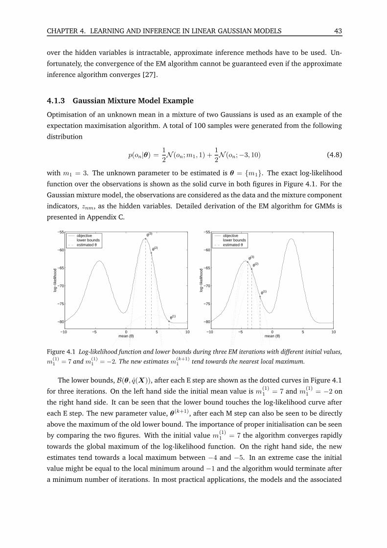
CHAPTER 4. LEARNING AND INFERENCE IN LINEAR GAUSSIAN MODELS 43
over the hidden variables is intractable, approximate inference methods have to be used. Un-
fortunately, the convergence of the EM algorithm cannot be guaranteed even if the approximate
inference algorithm converges [27].
4.1.3 Gaussian Mixture Model Example
Optimisation of an unknown mean in a mixture of two Gaussians is used as an example of the
expectation maximisation algorithm. A total of 100 samples were generated from the following
distribution
p(on|θ) =1
2N (on;m1, 1) +
1
2N (on;−3, 10) (4.8)
with m1 = 3. The unknown parameter to be estimated is θ = m1. The exact log-likelihood
function over the observations is shown as the solid curve in both figures in Figure 4.1. For the
Gaussian mixture model, the observations are considered as the data and the mixture component
indicators, znm, as the hidden variables. Detailed derivation of the EM algorithm for GMMs is
presented in Appendix C.
−10 −5 0 5 10
−80
−75
−70
−65
−60
−55
θ(1)
θ(2)
θ(3)
log−
likel
ihoo
d
mean (θ)
objective lower bounds estimated θ
−10 −5 0 5 10
−80
−75
−70
−65
−60
−55
θ(1)
θ(2)
θ(3)
log−
likel
ihoo
d
mean (θ)
objective lower bounds estimated θ
Figure 4.1 Log-likelihood function and lower bounds during three EM iterations with different initial values,
m(1)1 = 7 and m
(1)1 = −2. The new estimates m
(k+1)1 tend towards the nearest local maximum.
The lower bounds, B(θ, q(X)), after each E step are shown as the dotted curves in Figure 4.1
for three iterations. On the left hand side the initial mean value is m(1)1 = 7 and m
(1)1 = −2 on
the right hand side. It can be seen that the lower bound touches the log-likelihood curve after
each E step. The new parameter value, θ(k+1), after each M step can also be seen to be directly
above the maximum of the old lower bound. The importance of proper initialisation can be seen
by comparing the two figures. With the initial value m(1)1 = 7 the algorithm converges rapidly
towards the global maximum of the log-likelihood function. On the right hand side, the new
estimates tend towards a local maximum between −4 and −5. In an extreme case the initial
value might be equal to the local minimum around −1 and the algorithm would terminate after
a minimum number of iterations. In most practical applications, the models and the associated

CHAPTER 4. LEARNING AND INFERENCE IN LINEAR GAUSSIAN MODELS 44
log-likelihood functions are very complex and the chances of hitting a minimum during the
initialisation are close to zero.
4.2 Inference in Linear Gaussian Models
Inference involves deriving some knowledge about the state of a statistical model given a set
of observations. This knowledge may be needed, for example, in parameter estimation in the
form of posterior statistics over the hidden variables as seen in Section 4.1.2. In the case of
simple distributions, such as a Gaussian, the model has no meaningful state. In contrast a Gaus-
sian mixture model (GMM) may be viewed as having a discrete state indicating which mixture
component generated a given observation as described in Section 4.1.3. Inference for a GMM re-
quires evaluating the posterior probability mass function of the mixture component indicator. In
state space models, such as linear dynamical systems, the notion of a state is more obvious. Since
the states are not observed inference algorithms are required to evaluate the posterior distribu-
tion over the states given some observations. In the case of dynamic models with continuous
state vectors, three different forms may be identified. First, prediction is defined as estimating
the posterior over the hidden variables given some observations prior the current time instant.
Most often a one step prediction, p(xt|o1:t−1), is needed. Evaluating the posterior over the hid-
den variables given the observation sequence up to the current time instant, p(xt|o1:t), is called
filtering. Finally, evaluating the posterior given the complete observation sequence, p(xt|O), is
called smoothing.
For some models like the hidden Markov model in Chapter 2 and the linear dynamical system
in Chapter 3, the inference is tractable. In many models the observation likelihoods are not
Gaussians. This results in intractable integrals when estimating the posterior distribution over
the hidden variables. For the Gaussian mixture model the likelihoods are Gaussians if only the
mixture component indicator is hidden as seen in Section 4.1.3. However, the inference becomes
more complicated if one of the mean vectors, m1, in a GMM is unknown and the posterior of
m1 has to be estimated given the observations. For example, a mixture of two Gaussians with
known parameters apart from m1, the observation likelihood is
p(on|m1) =1
2N (on;m1, 1) +
1
2N (on;−3, 10) (4.9)
This is the same problem as in the EM example in Section 4.1.3. The inference examples in
the remainder of this chapter use the Bayesian learning framework. Given the prior distribution
for the mean vector is also a Gaussian m1 ∼ N (0, 100), the marginal likelihood for Bayesian
learning is given by
p(o1:N ) =
∫
p(m1)
N∏
n=1
p(on|m1)dm1 (4.10)
where the integrand is a mixture of 2N Gaussian product components. This exponential growth
in components renders the standard inference algorithms infeasible. Other examples are some

CHAPTER 4. LEARNING AND INFERENCE IN LINEAR GAUSSIAN MODELS 45
dynamic models, such as the switching linear dynamical system (SLDS), which has conditionally
Gaussian distributions and will be described in Chapter 6. This has led to the development of
approximate inference algorithms. Approximate inference algorithms may be divided into two
categories: deterministic and stochastic.
4.3 Approximate Inference: Deterministic Algorithms
The deterministic algorithms reviewed in this section are based on approximate distributions
which are made as close to the true distribution function as possible according to some optimality
criterion. Usually the Kullback-Leibler (KL) distance is used as this criterion. The KL distance
is first reviewed. Then three deterministic algorithms for approximate inference are described.
All these deterministic algorithms suffer from a major drawback: very little may be said about
the accuracy of the approximation. However, they are usually relatively fast compared to the
stochastic algorithms which are presented later in this chapter.
4.3.1 Kullback-Leibler Distance
The Kullback-Leibler distance may be used to measure the similarity of two densities, q(x) and
p(x). The KL distance is defined as the relative entropy of q(x) with respect to p(x) [127]
D(q(x), p(x)
)=
∫
q(x) logq(x)
p(x)dx (4.11)
This is a convex function of q(x), always non-negative, D(q(x), p(x)) ≥ 0, and equal to zero only
if q(x) = p(x). Note, as it does not satisfy the triangle inequality it is not a metric. For this
reason it is sometimes called the KL divergence.
The KL distance is important in many of the deterministic approximate inference algorithms.
It also provides an alternative derivation for the expectation step in the standard EM algorithm.
Instead of using the method of Lagrange multiplier in Section 4.1.1, it is sufficient to investigate
the difference between the log-likelihood function, L(θ), and the lower bound, B(θ, q(X)), in
Equation 4.3
L(θ) − B(θ, q(X)
)= log p(O|θ) −
∫
q(X) logp(O,X|θ)
q(X)dX
=
∫
q(X)(
log p(O|θ) − logp(O,X |θ)
q(X)
)
dX
=
∫
q(X) logq(X)
p(X |O,θ)dX = D
(q(X), p(X |O,θ)
)(4.12)
which is equal to zero only if q(X) = p(X |O,θ). Hence, minimising the KL distance between
q(X) and p(X |O,θ) is the same as minimising the difference between L(θ) and B(θ, q(X)). If
the posterior distribution over the hidden variables can be solved analytically, the difference is
zero and the lower bound in Equation 4.3 becomes an equality.

CHAPTER 4. LEARNING AND INFERENCE IN LINEAR GAUSSIAN MODELS 46
4.3.2 Moment Matching
The problem of estimating the posterior of the mean,m1, in Section 4.2 may be solved by approx-
imating the joint likelihood by a Gaussian, qn(m1) = N (m1;u, v). The dependence on the ob-
servation sequence is omitted since the function qn(m1) is only an approximation of p(m1|o1:n).
In assumed density filtering (ADF) [90] the observations are processed sequentially by updating
the approximate posterior according to the exact inference and projecting the resulting multiple
component distribution down to a single Gaussian using moment matching. Defining the ob-
servation terms as t0(m1) = p(m1) and tn(m1) = p(on|m1), and given the approximate density
after n−1 observations, qn−1(m1), another approximate density, pn(m1), is obtained by the exact
update
pn(m1) =tn(m1)qn−1(m1)
∫tn(m1)qn−1(m1)dm1
(4.13)
which is generally a mixture of two Gaussian product terms. The new approximate parame-
ter posterior, qn(m1), is found by matching the first two moments, Eqnm1 = Epnm1 and
Eqnm1m1 = Epnm1m1. This is also known as weak marginalisation and is the best ap-
proximation in the KL sense [74]. It may be shown that the moment matching is equivalent to
minimising the KL distance, D(pn(m1), qn(m1)). The ADF can be summarised as algorithm 2.
The exact formulae for the example may be found in a variety of studies [91, 94].
Algorithm 2 Assumed Density Filtering
initialise q0(θ) = t0(θ)
for n = 1 to N do
zn =∫tn(θ)qn−1(θ)dθ
pn(θ) = tn(θ)qn−1(θ)/zn
Eqnθ = Epnθ
Eqnθθ′ = Epnθθ′
end for
q(θ) = qN(θ)
It should be noted that the order of the observations influence the final estimate in the ADF
algorithm. The normalising constants, zn, may be used to approximate the joint likelihood of the
data as p(o1:N ) ≈∏
n zn. Two estimates for the mean, m1, in the GMM example with different
ordering of the observations are shown on the left hand side in Figure 4.2. In the first setup the
estimated parameter, θ(1), is close to the local maximum. In the second setup the estimate, θ(2),
is close to the prior mean. Thus, the algorithm has performed poorly.
Moment matching has also been applied to dynamic models such as SLDS [8]. The scheme
for SLDS corresponding to ADF for independent observations is called generalised pseudo Bayesian
algorithm of order 1. Though it may seem obvious that the errors introduced at each time step
tend to accumulate, it has been shown [15] that the final error is bounded. The stochastic
process ensures that the variance of the true distribution is high enough to overlap with the

CHAPTER 4. LEARNING AND INFERENCE IN LINEAR GAUSSIAN MODELS 47
approximate distribution.
−10 −5 0 5 10
−80
−75
−70
−65
−60
−55
θ(1)
θ(2)
log−
likel
ihoo
d
mean (θ)
objective ADF estimated θ
−10 −5 0 5 10
−80
−70
−60
−50
−40
−30
−20 θ
log−
likel
ihoo
d
mean (θ)
objective EP estimated θ
Figure 4.2 Assumed density filtering and expectation propagation in the Bayesian learning example for the
mean of a Gaussian mixture model. Two different orderings of the observations in ADF result in the estimates
θ(1) and θ(2). The EP algorithm arrives at a good estimate provided it converges at all due to the multimodal
posterior.
4.3.3 Expectation Propagation
Expectation propagation (EP) [91] addresses the shortcomings in assumed density filtering.
Provided the posterior is approximated by any distribution in the exponential family, the ADF
algorithm may be viewed as approximating the observation terms, tn(θ), instead of the updated
posteriors, pn(θ). The approximate observation terms can be defined as
tn(θ) = znq(θ)
qn−1(θ)(4.14)
where q(θ) is the approximate posterior for the whole set of observations. Since distributions
in the exponential family are closed in division, the approximate observation term has the same
functional form and may be evaluated analytically. Thus, it is always possible to remove the in-
fluence of any observation term from the final approximate posterior, q(θ), and refine the term,
tn(θ). In this way the order of the observations does not influence the final approximate poste-
rior as long as the refinements are iterated until convergence. The EP algorithm is summarised
in Algorithm 3.
The normalising constants, zn, may again be used to give an approximation to the joint like-
lihood of the observations given by p(o1:N ) ≈∫ ∏
n tn(θ)dθ. Unfortunately, the EP algorithm
performs well only if the posterior distribution is simple. If the posterior is multimodal, as in the
GMM example, some variances of the observation terms may get negative values. The variances
may be restricted to have positive values [90], but this results in inaccurate estimates and con-
vergence problems with some orderings of the observations. The results of the EP algorithm in
the GMM example are shown on the right hand side in Figure 4.2. The estimate for the unknown

CHAPTER 4. LEARNING AND INFERENCE IN LINEAR GAUSSIAN MODELS 48
Algorithm 3 Expectation Propagation
initialise tn(θ)
q(θ) =Q
n tn(θ)R
Q
n tn(θ)dθ
repeat
for n = 1 to N do
qn−1(θ) ∝ q(θ)/tn(θ)
zn =∫tn(θ)qn−1(θ)dθ ADF starts
pn(θ) = tn(θ)qn−1(θ)/zn
Eqθ = Epnθ
Eqθθ′ = Epnθθ′ ADF ends
tn(θ) = znq(θ)/qn−1(θ)
end for
until all tn(θ) converge
mean is quite accurate, but the approximation of p(o1:N ) is worse due to the restricted variances.
Exact formulae for the example may be found in a variety of studies [91, 94].
4.3.4 Variational Methods
Variational methods have recently been introduced to carry out approximate inference in graph-
ical models [64]. If the posterior distribution over the hidden variables is intractable and it has
to be approximated, the bound in Equation 4.3 never reaches equality. Instead, by introducing
a variational approximation over the hidden variables, q(X), which has a tractable form, the
lower bound may be maximised by minimising the Kullback-Leibler distance between the ap-
proximate distribution and the posterior, L(θ)−B(θ, q(X)) = D(q(X), p(X |O,θ)). The tightest
possible bound is found by varying the parameters of q(X), known as variational parameters.
The variational approximation does not always have to be the simplest density function, since
the model often has tractable substructures if some arcs in the corresponding Bayesian network
are removed [121].
In the context of Bayesian learning the variational methods are often called variational Bayes.
For the GMM example, two hidden variables may be identified: the mixture indicator and the
unknown mean. The log-likelihood over the observations may be bounded as follows
log p(O) ≥∑
∀Z
∫
q(Z,m1) logp(O,Z,m1)
q(Z,m1)dm1 (4.15)
where Z is a matrix of mixture indicators znm defined in Appendix C. Following the derivations
in various studies [3, 92], the variational approximation is constrained to factor q(Z,m1) =
q(Z)q(m1) where the mixture indicator probability may be further simplified to
q(znm) ∝ P (ω = m) exp(∫
q(m1) log p(on|ω = m,m1)dm1
)
(4.16)

CHAPTER 4. LEARNING AND INFERENCE IN LINEAR GAUSSIAN MODELS 49
and the mean distribution is chosen to be a Gaussian, q(m1) = N (m1;u, v). The variational
Bayes algorithm alternates between estimating the mixture indicator probability and the mean
distribution until the bound in Equation 4.15 is minimised. The results of variational Bayes
estimation in the GMM example are shown on the left hand side in Figure 4.3 for two different
prior mean values, u = −2 and u = 0. The estimates are accurate in this example but the
algorithm only finds the local maximum depending on the initialisation of the prior mean.
−10 −5 0 5 10
−80
−75
−70
−65
−60
−55
θ(1)
θ(2)
log−
likel
ihoo
d
mean (θ)
objective VB estimated θ
−10 −5 0 5 10
−80
−75
−70
−65
−60
−55
log−
likel
ihoo
d
mean (θ)
objective importance weightsestimated θ
Figure 4.3 Variational Bayes and importance sampling in the Bayesian learning example for the mean of a
Gaussian mixture model. Two different prior mean values, m = −2 and m = 0, in variational Bayes result
in different estimates, θ(1) and θ(2). The importance sampling is not challenged by the multimodal posterior
distribution.
4.4 Approximate Inference: Stochastic Algorithms
The deterministic inference algorithms in Section 4.3 are restricted to approximating the poste-
rior distributions by Gaussians or other distributions in the exponential family. These approaches
are fast but accuracy decreases if the posterior distributions are non-Gaussian as seen in some
of the GMM examples. Stochastic algorithms based on Monte Carlo methods assume little about
the posterior distribution. Instead of using the lower bounds or any deterministic optimality
criteria, Monte Carlo methods are based on drawing samples from the posterior distribution
and evaluating the required statistics using these samples. Generally, Monte Carlo methods are
computationally more intensive than the deterministic approximations. Schemes to make the
sampling more efficient will be presented later in this work.
4.4.1 Monte Carlo Methods
Monte Carlo methods may be used to approximate expectations of functions under distributions
which cannot be analytically solved. Two problems arise in this simulation based approach.
Firstly, how to draw samples from a given probability density function. Secondly, how to approx-
imate expectations under these distributions. Given N samples, x(1), . . . , x(N), a probability

CHAPTER 4. LEARNING AND INFERENCE IN LINEAR GAUSSIAN MODELS 50
density function may be approximated with the following empirical point-mass function
pN (x) =1
N
N∑
n=1
δ(x− x(n)) (4.17)
where δ(x−x(n)) denotes the Dirac delta function centred around the sample x(n). Consequently,
the expectations (integrals), I(f), of functions, f(x), under the distribution can be approximated
with tractable sums
IN (f) =1
N
N∑
n=1
f(x(n)) −→N→∞
I(f) =
∫
f(x)p(x)dx (4.18)
which are unbiased and by the strong law of large numbers will converge almost surely1 as N
tends to infinity [112].
The first problem is how to draw samples from a given probability density function. This
is straightforward only if the density, p(x), is of a standard form, for example, in a Gaussian
distribution or in a discrete probability mass function. Otherwise, Monte Carlo methods includ-
ing rejection sampling, importance sampling or Markov chain Monte Carlo (MCMC) algorithms
have to be used [86]. As an example of classical Monte Carlo methods, importance sampling
is considered. Importance sampling is also of fundamental importance in modern sequential
Monte Carlo and particle filter theory [27, 28, 61].
Importance sampling is based on drawing samples from a proposal distribution q(x). As
long as the proposal distribution and the objective are non-zero in the same region; that is,
p(x) ≤ Zq(x), Z <∞, an integral under the distribution p(x) may be written as
I(f) =
∫
f(x)w(x)q(x)dx (4.19)
where the importance weights are defined as w(x) = p(x)q(x) . An approximation of the density p(x)
using N samples may be expressed as
pN (x) =N∑
n=1
w(x(n))δ(x − x(n)) (4.20)
and any integral under p(x) may be approximated by
IN (f) =N∑
n=1
w(x(n))f(x(n)) (4.21)
The importance sampling algorithm is summarised in Algorithm 4.
The efficiency of importance sampling depends on the choice of the proposal distribution.
For the GMM example the prior distribution, p(m1) = N (0, 100), may be used as the proposal
distribution. The results of importance sampling with N = 100 are shown on the right hand side
in Figure 4.3. It is easy to see that importance sampling is very little challenged by the multi-
modal distribution in finding the global maximum and provides the best parameter estimate in
the Bayesian learning example.
1Almost sure convergence is also known as probability-1 convergence.

CHAPTER 4. LEARNING AND INFERENCE IN LINEAR GAUSSIAN MODELS 51
Algorithm 4 Importance Sampling
draw N samples, x(1), . . . , x(N), from q(x)
evaluate importance weights w(x(n)) = p(x(n))
q(x(n))
evaluate any approximate integral required IN (f) =∑N
n=1w(x(n))f(x(n))
4.4.2 Markov Chain Monte Carlo Methods
Importance sampling only works well if the proposal distribution q(x) is a good approximation
to p(x). In complex problems with high dimensional distributions it is difficult to create a single
density q(x) that has this property [86]. Markov chain Monte Carlo (MCMC) methods generate
samples x(n) while exploring the state space using a Markov chain mechanism. This mechanism
is constructed so that the chain spends more time in the most important regions. The MCMC
algorithms are especially suitable for state space models with Markov dynamics.
Gibbs sampling is one instance of Markov chain Monte Carlo methods for sampling from
distributions over at least two dimensions [112]. It is assumed that whilst p(x) is too complex to
draw samples from directly, its conditional distributions, p(xj|x(n)−j ) where x
(n)−j = x
(n)1 , . . . , x
(n)j−1,
x(n−1)j+1 , . . . , x
(n−1)N , can be used as proposal distributions. The superscript refers to the nth
iteration. For many graphical models these conditional distributions are easy to sample from.
In general, a single iteration of Gibbs sampling involves sampling one parameter at a time as
follows2
x(n)j ∼ p(xj |x
(n)−j ) (4.22)
After Ni iterations the final estimates are computed in common with all Monte Carlo methods
pNi(x) =
1
Ni
Ni∑
n=1
δ(x − x(n)) (4.23)
which converge towards its invariant density function, p(x), if the Markov chain is irreducible
and aperiodic [1]. Gibbs sampling explores the state space by a random walk steered by the
conditional distributions. It may be slow to converge if the state space is large. Sometimes the
structure of the model allows efficient sampling by separating tractable substructures and thus
drawing samples in a lower dimensional state space. The general Gibbs sampling algorithm is
summarised in Algorithm 5.
As an example of Gibbs sampling a two dimensional Gaussian distribution is considered.
Although, the density function is tractable and its mean vector may be easily estimated from
the sample mean, it provides a simple illustration of how the algorithm works. For a correlated
two dimensional distribution, as shown by the contours of equal probability in Figure 4.4, the
conditional distributions p(x1|x2) and p(x2|x1) may be easily derived using the results from
2In the case of Monte Carlo methods, the ∼ symbol is used to indicate that the sample on the left hand side was
drawn from the density function on the right hand side. The samples, which always have the superscript as in x(n)j ,
should not be confused with random variables.

CHAPTER 4. LEARNING AND INFERENCE IN LINEAR GAUSSIAN MODELS 52
Algorithm 5 Gibbs Sampling
initialise x(1)
for n = 2 to Ni do
Draw a sample x(n)j ∼ p(xj |x
(n)−j ) for all j
end for
evaluate any approximate integral required INi(f) =
∑Ni
n=1 f(x(n))
−10 −5 0 5 10−10
−8
−6
−4
−2
0
2
4
6
8
10
x1
x 2
Figure 4.4 Gibbs sampling example for 8 full iterations. The initial value of the sample is x(0) = [3,−3]′.
The dashed line follows all the sampling steps, [x(0)1 , x
(0)2 ]′, [x
(1)1 , x
(0)2 ]′, [x
(1)1 , x
(1)2 ]′, [x
(2)1 , x
(1)2 ]′, . . ..
Appendix B. All the steps of Gibbs sampling are illustrated by the dashed line in the figure.
The black dots represent the samples for each of 8 iterations. For this example the algorithm
converged fast and the mean vector may be easily estimated as the average of the samples.
Sometimes the first Nb samples, which is called the burn in period, are discarded to obtain
samples independent of the initialisation [86].
4.5 Summary
This chapter has reviewed the expectation maximisation algorithm for parameter optimisation.
The EM algorithm may be used to find the maximum likelihood estimates for the parameters of
many linear Gaussian models described in Chapter 3. In the expectation step, the posterior dis-
tribution of the hidden variables in the model given the sequence of observations is evaluated.
The evaluation of these posteriors is also known as inference. For some models inference is not

CHAPTER 4. LEARNING AND INFERENCE IN LINEAR GAUSSIAN MODELS 53
feasible due to intractable integrals involved in the evaluation. A number of approximate infer-
ence algorithms were reviewed. Two classes of approximate inference schemes were considered,
deterministic and stochastic. The deterministic algorithms are based on approximating the exact
posterior distributions with tractable densities. These densities are usually Gaussians which may
be a poor approximation for complex posterior distributions. The stochastic algorithms such as
Markov chain Monte Carlo assume little about the form of the posterior, but are often compu-
tationally more demanding than the deterministic algorithms. However, the efficiency of the
MCMC algorithms may be increased by careful design of the proposal mechanism; for example,
Rao-Blackwellisation reviewed later in this work.

5
Piece-Wise Constant State Evolution
In this chapter a state space model based on an underlying hidden Markov model with factor
analysis observation process is introduced. The HMM generates a piece-wise constant state
evolution process as discussed in Chapter 3. The observations are produced from the state
vectors by a factor analysis observation process. The model is called a factor analysed HMM
(FAHMM). Firstly, the theory of FAHMMs is presented including the form of the generative
model and likelihood calculation. Maximum likelihood estimation of the FAHMM parameters
using expectation maximisation algorithm is then presented. Due to the flexibility of FAHMMs,
many configurations correspond to standard systems. Finally, implementation issues including
initialisation, parameter sharing and numerical accuracy are considered.
5.1 Factor Analysed Hidden Markov Models
Factor analysis was described in Chapter 3 as an example of a static linear Gaussian model.
Standard factor analysis may be extended to employ Gaussian mixture models as the observa-
tion noise. This is called shared factor analysis [46]. In factor analysed hidden Markov models
the factors (state vector) are generated by an underlying mixture of Gaussians HMM. The obser-
vation process parameters are chosen by the current HMM state.
5.1.1 Generative Model of FAHMM
The factor analysed hidden Markov model is a dynamic state space generalisation of a multiple
component factor analysis system. The k-dimensional state vectors are generated by a standard
diagonal covariance Gaussian mixture HMM. The p-dimensional observation vectors are gener-
ated by a multiple noise component factor analysis observation process. A generative model for
the FAHMM can be described as follows1
1The ∼ symbol in qt ∼ P (qt|qt−1) is used to represent a discrete Markov chain. Normally it means the variable on
the left hand side is distributed according to the probability density function on the right hand side as in x ∼ N (µ,Σ).
54

CHAPTER 5. PIECE-WISE CONSTANT STATE EVOLUTION 55
qt ∼ P (qt|qt−1)
xt = wqt, wj ∼∑
n
c(x)jn N (µ
(x)jn ,Σ
(x)jn )
ot = Cqtxt + vqt , vj ∼∑
m
c(o)jmN (µ
(o)jm,Σ
(o)jm)
(5.1)
The HMM state transition probabilities from state i to state j are represented by aij and the state
and observation space mixture distributions are described by the mixture weights c(x)jn , c
(o)jm,
mean vectors µ(x)jn ,µ
(o)jm and diagonal covariance matrices Σ
(x)jn ,Σ
(o)jm.
xt xt+1
ot ot+1
t+1qqt
ω t(x) ωt+1
(x)
ω t(o) ωt+1
(o)
Figure 5.1 Dynamic Bayesian network representing a factor analysed hidden Markov model.
Dynamic Bayesian networks (DBN), described in Chapter 3, may be presented in conjunc-
tion with the generative models to illustrate the conditional independence assumptions made
in a statistical model. A DBN describing a FAHMM is shown in Figure 5.1. The square nodes
represent discrete random variables such as the HMM state qt, and ω(x)t , ω
(o)t which indi-
cate the active state and observation mixture components, respectively. Continuous random
variables such as the state vectors, xt, are represented by round nodes. Shaded nodes depict
observable variables, ot, leaving all the other FAHMM variables hidden. A conditional indepen-
dence assumption is made between variables that are not connected by directed arcs. The state
conditional independence assumption between the output densities of a standard HMM is also
used in a FAHMM.
5.1.2 FAHMM Likelihood Calculation
An important aspect of any generative model is the complexity of the likelihood calculations. The
generative model in Equation 5.1 can be expressed by the following two Gaussian distributions
p(xt|qt = j, ω(x)t = n) = N (xt;µ
(x)jn ,Σ
(x)jn ) (5.2)
p(ot|xt, qt = j, ω(o)t = m) = N (ot;Cjxt + µ
(o)jm,Σ
(o)jm) (5.3)

CHAPTER 5. PIECE-WISE CONSTANT STATE EVOLUTION 56
The likelihood of an observation ot given the state qt = j, state space component ω(x)t = n and
observation noise component ω(o)t = m can be obtained by integrating the state vector xt out
of the product of the above Gaussians. The resulting likelihood is also a Gaussian and can be
written as
bjmn(ot) = p(ot|qt = j, ω(o)t = m,ω
(x)t = n) = N
(ot;µjmn,Σjmn
)(5.4)
where
µjmn = Cjµ(x)jn + µ
(o)jm (5.5)
Σjmn = CjΣ(x)jn C ′
j + Σ(o)jm (5.6)
Hence, the conditional observation density of a FAHMM state j can be viewed as an M (o)M (x)
component full covariance matrix GMM with mean vectors given by Equation 5.5 and covariance
matrices given by Equation 5.6.
The likelihood calculation requires inverting M (o)M (x) full p by p covariance matrices in
Equation 5.6. If the amount of memory is not an issue, the inverses and the corresponding
determinants for all the discrete states in the system can be computed prior to starting off with
a training iteration or recognition. However, this can rapidly become impractical for a large
system. A more memory efficient implementation requires the computation of the inverses and
determinants for each time instant. These can be efficiently obtained using the following equality
for matrix inverses [52]
(CjΣ(x)jn C ′
j + Σ(o)jm)−1 = Σ
(o)−1jm −Σ
(o)−1jm Cj(C
′jΣ
(o)−1jm Cj + Σ
(x)−1jn )−1C ′
jΣ(o)−1jm (5.7)
where the inverses of the covariance matrices Σ(o)jm and Σ
(x)jn are trivial to compute since they are
diagonal. The full matrix, C ′jΣ
(o)−1jm Cj + Σ
(x)−1jn , requires only a k by k matrix to be inverted.
This is faster than inverting full p by p matrices if k p. The determinants needed in the
likelihood calculations can be obtained using the following equality [52]
|CjΣ(x)jn C ′
j + Σ(o)jm| = |Σ
(o)jm||Σ
(x)jn ||C
′jΣ
(o)−1jm Cj + Σ
(x)−1jn | (5.8)
where the determinants of the diagonal covariance matrices are trivial to compute and often
the determinant of the k by k matrix is obtained as a by-product of its inverse; for example
using Cholesky decomposition [127]. In a large system, a compromise has to be made between
precomputing the inverse matrices and computing them for each time instant. For example,
caching of the inverses can be employed, because some components are likely to be computed
more often than others when pruning is used.
The Viterbi algorithm [125] can be used to produce the most likely state sequence in the
same way as with standard HMMs as described in Chapter 2. The likelihood of an observation
ot given only the state qt = j can be obtained by marginalising the likelihood in Equation 5.4 as
follows
bj(ot) = p(ot|qt = j) =
M(o)∑
m=1
c(o)jm
M(x)∑
n=1
c(x)jn bjmn(ot) (5.9)

CHAPTER 5. PIECE-WISE CONSTANT STATE EVOLUTION 57
Any Viterbi algorithm implementation, such as the token passing algorithm [131], can easily be
modified to support FAHMMs in this way. The modifications to the forward-backward algorithm
are discussed in the following training section.
5.1.3 Optimising FAHMM Parameters
The maximum likelihood (ML) criterion may be used to optimise the FAHMM parameters. It is
also possible to find a discriminative training scheme such as minimum classification error [122].
However, in this work only ML training is considered. In common with standard HMM training
described in Chapter 2 the expectation maximisation (EM) algorithm is used. The auxiliary
function for FAHMMs can be written as
Q(θ,θ(k)) =∑
∀Q
∫
P (Q|O,θ(k))p(X |O, Q,θ(k)) log p(O,X , Q|θ)dX (5.10)
where all the possible discrete state and continuous state sequences of length T are included in
the sum and the integral. A sequence of observation vectors is denoted by O = o1, . . . ,oT ,
and X = x1, . . . ,xT is a sequence of state vectors. The set of current model parameters is
represented by θ(k).
Sufficient statistics for the first term, P (Q|O,θ(k)), in the auxiliary function in Equation
5.10 can be obtained using the standard forward-backward algorithm described in Chapter 2
with likelihoods given by Equation 5.9. For the state transition probability optimisation, two
sets of sufficient statistics are needed, the posterior probabilities of being in state j at time
t, γj(t) = P (qt = j|O,θ(k)), and being in state i at time t − 1 and in state j at time t, ξij(t) =
P (qt−1 = i, qt = j|O,θ(k)). For the state conditional observation density parameter optimisation,
the component posteriors, γjmn(t) = P (qt = j, ω(o)t = m,ω
(x)t = n|O,θ(k)), have to be estimated.
These can be obtained within the forward-backward algorithm as follows
γjmn(t) =1
p(O|θ(k))
Ns∑
i=1
aijαi(t− 1)c(o)jmc
(x)jn bjmn(ot)βj(t) (5.11)
where Ns is the number of HMM states in the model, αi(t− 1) is the standard forward and βj(t)
is the standard backward variable defined for HMMs in Chapter 2.
The second term, p(X|O, Q,θ(k)), in the auxiliary function in Equation 5.10 is the state
vector distribution given the observation sequence and the discrete state sequence. Only the
first and second-order statistics are required since the distributions are conditionally Gaussian
given the state and the mixture components. Using the conditional independence assumptions
made in the model, the posterior can be expressed as
p(xt|ot, qt = j, ω(o)t = m,ω
(x)t = n) =
p(ot,xt|qt = j, ω(o)t = m,ω
(x)t = n)
p(ot|qt = j, ω(o)t = m,ω
(x)t = n)
(5.12)
which using Equations 5.2, 5.3 and 5.4 simplifies to a Gaussian distribution with mean vector,

CHAPTER 5. PIECE-WISE CONSTANT STATE EVOLUTION 58
xjmnt, and correlation matrix, Rjmnt, defined by
xjmnt = µ(x)jn + Kjmn(ot − Cjµ
(x)jn − µ
(o)jm) (5.13)
Rjmnt = Σ(x)jn − KjmnCjΣ
(x)jn + xjmntx
′jmnt (5.14)
where Kjmn = Σ(x)jn C ′
j
(CjΣ
(x)jn C ′
j + Σ(o)jm
)−1. It should be noted that the matrix inverted in
the equation for Kjmn is the inverse covariance matrix in Equation 5.7 and the same efficient
algorithms presented in Section 5.1.2 apply.
Given the two sets of sufficient statistics above the model parameters can be optimised by
solving a standard maximisation problem. The parameter update formulae for the underlying
HMM parameters in FAHMM are very similar to those for the standard HMM [129] except the
above state vector distribution statistics replace the observation sample moments. Omitting the
state transition probabilities, the state space parameter update formulae can be written as
c(x)jn =
T∑
t=1
M(o)∑
m=1
γjmn(t)
T∑
t=1
γj(t)
(5.15)
µ(x)jn =
T∑
t=1
M(o)∑
m=1
γjmn(t)xjmnt
T∑
t=1
M(o)∑
m=1
γjmn(t)
(5.16)
Σ(x)jn = diag
(
T∑
t=1
M(o)∑
m=1
γjmn(t)Rjmnt
T∑
t=1
M(o)∑
m=1
γjmn(t)
− µ(x)jn µ
(x)′jn
)
(5.17)
where diag(·) sets all the off-diagonal elements of the matrix argument to zeros. The cross
terms including the new state space mean vectors and the first-order accumulates have been
simplified in Equation 5.17. This can only be done if the mean vectors are updated during the
same iteration, and the covariance matrices and the mean vectors are tied on the same level.
Parameter tying is further discussed in Section 5.2.2.
The new observation matrix, Cj , has to be optimised row by row as in SFA [48]. The scheme
adopted in this work closely follows the maximum likelihood linear regression (MLLR) transform
matrix optimisation [33]. The lth row vector cjl of the new observation matrix can be written
as
cjl = k′jlG
−1jl (5.18)

CHAPTER 5. PIECE-WISE CONSTANT STATE EVOLUTION 59
where the k by k matrix Gjl and the k-dimensional column vector kjl are defined as follows
Gjl =M(o)∑
m=1
1
σ(o)2jml
T∑
t=1
M(x)∑
n=1
γjmn(t)Rjmnt (5.19)
kjl =
M(o)∑
m=1
1
σ(o)2jml
T∑
t=1
M(x)∑
n=1
γjmn(t)(otl − µ
(o)jml
)xjmnt (5.20)
where σ(o)2jml is the lth diagonal element of the observation covariance matrix Σ
(o)jm, otl and µ
(o)jml
are the lth elements of the current observation and the observation noise mean vectors, respec-
tively.
Given the new observation matrix, the observation noise parameters can be optimised using
the following formulae
c(o)jm =
T∑
t=1
M(x)∑
n=1
γjmn(t)
T∑
t=1
γj(t)
(5.21)
µ(o)jm =
T∑
t=1
M(x)∑
n=1
γjmn(t)(ot − Cjxjmnt
)
T∑
t=1
M(x)∑
n=1
γjmn(t)
(5.22)
Σ(o)jm =
1
T∑
t=1
M(x)∑
n=1
γjmn(t)
T∑
t=1
M(x)∑
n=1
γjmn(t)diag(
oto′t −
[
Cj µ(o)jm
][
xjmnto′t
o′t
]
−[
otx′jmnt ot
][
C′j
µ(o)′jm
]
+[
Cj µ(o)jm
][
Rjmnt xjmnt
x′jmnt 1
] [
C′j
µ(o)′jm
])
(5.23)
Detailed derivation of the parameter optimisation can be found in Appendix D.
A direct implementation of the training algorithm is inefficient due to the heavy matrix com-
putations required to obtain the state vector statistics. An efficient two level implementation
of the training algorithm is presented in Section 5.2.4. Since the noise covariance matrices are
assumed to be diagonal there is no need to compute the off-diagonal elements in Equations 5.17
and 5.23.
5.1.4 Standard Systems Related to FAHMMs
A number of standard systems can be related to FAHMMs. Since the FAHMM training algorithm
described above is based on the EM algorithm, it is only applicable if there is observation noise.

CHAPTER 5. PIECE-WISE CONSTANT STATE EVOLUTION 60
Some of the related systems have the observation noise set to zero, which means that different
optimisation methods have to be used. The related systems are presented in Table 5.1 and their
properties are further discussed below.
Table 5.1 Standard systems related to FAHMMs. FAHMM can be converted to the systems on the left hand
side by applying the restrictions on the right.
System Relation to FAHMMs
HMM M (x) = 0
SFA M (x) = 1
dynamic IFA M (o) = 1
STC k = p and vt = 0
Covariance EMLLT k > p and vt = 0
• By setting the number of state space mixture components to zero, M (x) = 0, FAHMM
reduces to a standard diagonal covariance Gaussian mixture HMM. The observation noise
acts as the state conditional output density of the HMM, and the observation matrix is
made redundant because no state vectors will be generated.
• By setting the number of state space mixture components to one, M (x) = 1, FAHMM
corresponds to SFA [48]. Even though the continuous state space distribution parameters
are modelled explicitly, there are effectively an equal number of free parameters in this
FAHMM and SFA which assumes a continuous state distribution with a zero mean and an
identity covariance matrix.
• By setting the number of observation space distribution components to one, M (o) = 1,
FAHMM corresponds to a dynamic version of IFA [2]. The only difference to the stan-
dard IFA is the independent state vector element (factor) assumption which would require
a multiple stream (factorial) HMM [43] with 1-dimensional streams in the state space.
Effectively, multiple streams can model a larger number of distributions, but the inde-
pendence assumption is relaxed in this FAHMM, assuming uncorrelated factors instead of
independent.
• By setting the observation noise to zero, vt = 0, and setting the state space dimensionality
equal to the observation space dimensionality, k = p, FAHMM reduces to a semi-tied
covariance matrix HMM. The only difference to the original STC model [34] is that the
mean vectors are also transformed in a FAHMM.
• By setting the observation noise to zero, vt = 0, and setting the state space dimensionality
to greater than the observation space dimensionality, k > p, FAHMM becomes a covariance
version of the extended maximum likelihood linear transformation (EMLLT) [99] scheme
described in Chapter 2. The FAHMM is based on a generative model which requires every

CHAPTER 5. PIECE-WISE CONSTANT STATE EVOLUTION 61
state space covariance matrix to be a valid covariance matrix; that is, positive definite.
However, EMLLT directly models the inverse covariance (precision) matrices and allows
“negative” variance elements as long as the resulting inverse covariance matrices are valid.
5.2 Implementation Issues
When factor analysed HMMs are used for large vocabulary continuous speech recognition (LVCSR)
there are a number of efficiency issues that must be addressed. As EM training is being used to
iteratively find the ML estimates of the model parameters, an appropriate initialisation scheme
is essential. Furthermore, in common with standard LVCSR systems, parameter tying may be
required for robust parameter estimation. In addition, there are a large amount of matrix oper-
ations that need to be computed. Issues with numerical accuracy have to be considered. Finally,
as there are two sets of hidden variables in FAHMMs, an efficient two level training scheme is
presented.
5.2.1 Initialisation
One major issue with the EM algorithm is that there may be a number of local maxima. An
appropriate initialisation scheme may improve the chances of finding a good solution. A sensible
starting point is to use a standard HMM. Although this maybe a local maximum for the trained
HMM, the experiments later in this work show that this is not the case for the initial FAHMM.
A single Gaussian mixture component HMM can be converted to an equivalent FAHMM when
k ≤ p as follows
µ(x)j = µj[1:k] (5.24)
Σ(x)j =
1
2Σj[1:k] (5.25)
µ(o)j =
[
0
µj[k+1:p]
]
(5.26)
Σ(o)j =
[12Σj[1:k] 0
0 Σj[k+1:p]
]
(5.27)
Cj =
[
I [k]
0
]
(5.28)
where I [k] is a k by k identity matrix, µj[1:k] represents the first k elements of the mean vector
and Σj[1:k] is the upper left k by k submatrix of the covariance matrix associated with state j
of the initial HMM. As an example initialisation for FAHMM with k = 2p, the following may be

CHAPTER 5. PIECE-WISE CONSTANT STATE EVOLUTION 62
used
µ(x)j =
[
µj
0
]
(5.29)
Σ(x)j =
[14Σj 0
014Σj
]
(5.30)
µ(o)j = 0 (5.31)
Σ(o)j =
1
2Σj (5.32)
Cj =[
I [k] I [k]
]
(5.33)
Initialisation schemes for an arbitrary k may be found by combining these two approaches.
The above initialisation schemes guarantee that the average log-likelihood of the training
data is equal to the one obtained using the original HMM. The equivalent FAHMM system can
also be obtained by setting the observation matrices equal to zero and initialising the observation
noise as the HMM output densities. However, the proposed method can be used to give more
weight on certain dimensions and can provide better convergence. Here it is assumed that the
first k observation vector elements are the most significant. In the experiments, the state space
dimensionality was often chosen to be k = 13, which corresponds to the static parameters in a
standard 39-dimensional observation vector.
Alternative observation vector element selection techniques such as the Fisher ratio [63] can
also be used within this initialisation scheme. For the Fisher ratio, within and between class
(state) covariance matrices have to be calculated. The within class covariance is defined as
Σ(w) =
1
Ns
Ns∑
j=1
(∑T
t=1 γj(t)(ot − µj)(ot − µj)′
∑Tt=1 γj(t)
)
(5.34)
where Ns is the total number of states in the system. The between class covariance is given by
Σ(b) =
1
Ns
Ns∑
j=1
(µj − µg)(µj − µg)′ (5.35)
where µg is the global mean of the data. The Fisher ratio for the ith observation vector element
is given by
Fi =Σ
(b)ii
Σ(w)ii
(5.36)
which is based on the assumptions that the elements of the observation vector are uncorrelated
and that the observation vectors within each class are Gaussian distributed with equal variance.
For the initialisation, observation vector elements with the highest Fisher ratio may be selected.
5.2.2 Parameter Sharing
As discussed in Section 3.5.2, the number of free parameters per FAHMM state, η, is the same
as a factor analysis with Gaussian mixture models. Table 5.2 summarises the numbers of free

CHAPTER 5. PIECE-WISE CONSTANT STATE EVOLUTION 63
parameters per HMM and FAHMM state2. Usually the dimensionality of the observation space is
p = 39 and the number of mixture components in a diagonal covariance HMM up to M (o) = 32.
The dimensionality of the state space, k, and the number of observation noise components,M (o),
have the largest influence on the complexity of FAHMMs.
Table 5.2 Number of free parameters per HMM and FAHMM state, η, using M (x) state space components,
M (o) observation noise components and no sharing of individual FAHMM parameters. Both diagonal covari-
ance and full covariance matrix HMMs are shown.
System Free Parameters (η)
diagonal covariance HMM 2M (o)p
full covariance HMM M (o)p(p+ 3)/2
FAHMM 2(M (x) − 1)k + pk + 2M (o)p
When context-dependent HMM systems are trained, the selection of the model set is of-
ten based on decision-tree clustering [7] as discussed in Chapter 2. However, implementing
decision-tree clustering for FAHMMs is not as straightforward as for HMMs. Clustering based
on single mixture component HMM statistics is not globally optimal for HMMs [98]. Since the
FAHMMs can be viewed as full covariance matrix HMMs, decision-tree clustered single mixture
component HMM models may be considered as a sufficiently good starting point for FAHMM
initialisation. The initialisation of the context-dependent models can be done the same way as
using standard context-independent HMMs described in Section 5.2.1.
In addition to state clustering, it is sometimes useful to share some of the individual FAHMM
parameters. It is possible to tie any number of parameters between an arbitrary number of mod-
els at various levels of the model. For example, the observation matrix can be shared globally or
between classes of discrete states as in semi-tied covariance HMMs [34]. A global observation
noise distribution could represent a stationary noise environment corrupting all the speech data.
Implementing arbitrary tying schemes is closely related to those used with standard HMM sys-
tems [129]. Sufficient statistics required for the tied parameter are accumulated over the entire
class sharing it before updating. If the mean vectors and the covariance matrices of the state
space noise are tied on a different level, all the cross terms between the first-order accumulates
and the updated mean vectors, µjn, have to be used in the covariance matrix update formula.
Equation 5.17, including all the cross terms, can be written as
Σ(x)jn = diag
(
T∑
t=1
M(o)∑
m=1
γjmn(t)(Rjmnt − xjmntµ
(x)′jn − µ
(x)jn x′
jmnt + µ(x)jn µ
(x)′jn
)
T∑
t=1
M(o)∑
m=1
γjmn(t)
)
(5.37)
where the first-order accumulates,∑
t
∑
m γjmn(t)xjmnt, may be different to those used for the
mean vector update in Equation 5.16.
2The mixture weights are discarded for brevity.

CHAPTER 5. PIECE-WISE CONSTANT STATE EVOLUTION 64
5.2.3 Numerical Accuracy
The matrix inversion described in Section 5.1.2 and the parameter estimation require many
matrix computations. Numerical accuracy may become an issue due to the vast amount of
sums of products. In the experiments it was found that double precision had to be used in all
the intermediate operations to guarantee that the full covariance matrices were non-singular.
Nevertheless, single precision was used to store the accumulates and model parameters due to
the issue of memory usage.
A large amount of training data is required to get reliable estimates for the covariance ma-
trices in a LVCSR system. Sometimes the new variance elements may become too small for
likelihood calculations. If any variance element becomes too small within the machine preci-
sion, a division by zero will occur. To avoid problems with FAHMMs the full covariance matrices
in Equation 5.6 must be guaranteed to be non-singular. The matrix C jΣ(x)jn C ′
j is at most rank k
provided the state space variances are valid. Therefore, it is essential that the observation noise
variances are floored properly. In the experiments it was found that the flooring scheme usu-
ally implemented in HMM systems [129] is sufficient for the observation variances in FAHMMs.
With very large model sets the new estimates for the state space variances may become negative
due to insufficient data for the component. In the experiments such variance elements were not
updated.
2 4 6 8 10
−100
−95
−90
−85full iteration 1
auxi
liary
func
tion
within iterations2 4 6 8 10
full iteration 2
within iterations2 4 6 8 10
full iteration 3
within iterations
Figure 5.2 Auxiliary function values versus within iterations during 3 full iterations of two level FAHMM
training.
5.2.4 Efficient Two Level Training
To increase the speed of training, a two level algorithm is adopted. The component specific first
and second-order statistics form the sufficient statistics required in the parameter estimation
described in Section 5.1.3. This can be verified by substituting the state vector statistics, xjmn(t)
and Rjmn(t), from Equations 5.13 and 5.14 into the update Equations 5.15-5.23. The sufficient

CHAPTER 5. PIECE-WISE CONSTANT STATE EVOLUTION 65
statistics can be written as
γjmn =T∑
t=1
γjmn(t) (5.38)
µjmn =
T∑
t=1
γjmn(t)ot (5.39)
Rjmn =
T∑
t=1
γjmn(t)oto′t (5.40)
Given these accumulates and the current model parameters, θ(k), the required accumulates for
the new parameters can be estimated. Since the estimated state vector statistics depend on
both the data accumulates and the current model parameters an extra level of iterations can be
introduced. After updating the model parameters, new state vector distribution given the old
data accumulates and the new model parameters can be estimated. These within iterations are
guaranteed to increase the log-likelihood of the data. Figure 5.2 illustrates the increase of the
auxiliary function values during three full iterations, 10 within iterations each.
0 2 4 6 8 10 12−76
−74
−72
−70
−68
−66
−64
−62
no. iterations
aver
age
log−
likel
ihoo
d
HMM baseline FAHMM one level training FAHMM two level training, 10 within iter
Figure 5.3 Average log-likelihood of the training data against the number of full iterations for baseline HMM
and an untied FAHMM with k = 13. One level training and more efficient two level training with 10 within
iterations were used.
The efficient training algorithm can be summarised as follows:
1. Collect the data statistics using forward-backward algorithm;

CHAPTER 5. PIECE-WISE CONSTANT STATE EVOLUTION 66
2. Estimate the state vector distribution p(xt|j,m, n,O,θ(k));
3. Estimate new model parameters θ;
4. If the auxiliary function value has not converged go to step 2 and update the parameters
θ → θ(k+1);
5. If the average log-likelihood of the data has not converged go to step 1 and update the
parameters θ → θ(k+1).
The within iterations decrease the number of full iterations needed in training. The overall
training time becomes shorter because less time has to be spent collecting the data accumu-
lates. The average log-likelihoods of the training data against the number of full iterations are
illustrated in Figure 5.3. Four iterations of embedded training were first applied to the baseline
HMM. The FAHMM system with k = 13 was initialised as described in Section 5.2.1. Both one
level training and more efficient two level training with 10 within iterations, were used and the
corresponding log-likelihoods are shown in the figure.
5.3 Summary
The factor analysed HMM was presented in this chapter. The FAHMM is based on a piece-
wise constant state evolution process and a factor analysis observation process as described
in the generalised linear Gaussian model framework in Chapter 3. The likelihood calculation
and the maximum likelihood parameter optimisation using the EM algorithm were presented.
Some configurations of the FAHMM were related to standard models used in speech recognition.
A number of implementation issues including initialisation and an efficient two level training
scheme were presented.

6
Linear Continuous State Evolution
In this chapter a state space model based on a linear first-order Gauss-Markov state evolution
process with discrete switching variable is described. This switching linear dynamical system
(SLDS) may be viewed as a combination of a hidden Markov model and a linear dynamical
system described in Chapter 3. The theory of SLDS using the generative model framework is
presented. The close relationship between this SLDS and the stochastic segment model (SSM)
is established. The inference algorithms for the SLDS are intractable. Hence, approximate infer-
ence algorithms described in Chapter 4 are presented with applications to SLDS. In particular, an
efficient approximate inference algorithm based on Gibbs sampling is presented. The algorithm
takes advantage of the tractable substructures in the SLDS to reduce the state space the samples
are drawn from. Also, an efficient proposal distribution with a complexity of O(T ) per iteration
is presented. Implementation issues for Gibbs sampling in speech recognition are also discussed.
6.1 Switching Linear Dynamical System
There has been interest in hybrid models since the formulation of efficient training and inference
algorithms for linear dynamical systems and hidden Markov models [8]. These hybrid models
have been called by many names such as switching Kalman filter [93, 95], conditionally Gaussian
model [16, 17], jump Markov linear system [26] and switching linear dynamical system [54,
103, 104, 134]. In this work, the term switching linear dynamical system is used due to its
intuitive connection to a linear dynamical system with switching parameters. The SLDS is closely
related to a stochastic segment model [24, 102] which uses linear dynamical systems as models
for observation dynamics within segments. However, the SSM uses an explicit duration model
and a number of LDSs per segment.
The SLDS may also be viewed as an extension to a factor analysed HMM by adding a better
model for inter-frame correlation. In the SSM the segments are assumed to be independent. The
continuous state vector is reset according to the initial state distribution in the segment bound-
aries. The original SSM also had multiple invariant regions within segments [24]. As the num-
ber of invariant regions in this SSM is increased the system starts converging towards FAHMM.
67

CHAPTER 6. LINEAR CONTINUOUS STATE EVOLUTION 68
Thus, SLDS should provide a better model for inter-frame correlation and co-articulation be-
tween modelling units, because the state vector is propagated over the segment boundaries.
6.1.1 Generative Model of SLDS
In SLDS the state vectors evolve according to a first-order Gauss-Markov process. The generative
model for a SLDS can be expressed as1
qt ∼ P (qt|qt−1)
xt = Aqtxt−1 + wqt , wj ∼∑
n
c(x)jn N (µ
(x)jn ,Σ
(x)jn )
ot = Cqtxt + vqt, vj ∼∑
m
c(o)jmN (µ
(o)jm,Σ
(o)jm)
(6.1)
where both the state transition matrix, Aj , and the observation matrix, C j, are chosen by the
discrete state, qt = j, and the state evolution and observation noises are Gaussian or Gaussian
mixture model distributed as in the factor analysed HMM presented in Chapter 5. The initial
continuous state is also Gaussian distributed, x1 ∼ N (µ(i)j ,Σ
(i)j ). The standard LDS reviewed
in Chapter 3 uses single Gaussian distributions as the state evolution and the observation noise.
The SLDS training presented later in this chapter can also handle GMMs as the noise sources.
The number of model parameters per state is η = (2 + 2M (x) + k)k + (2M (o) + k)p.
In addition to the generative models, the conditional independence assumptions made in
the model can be illustrated by the dynamic Bayesian network (DBN) on the right hand side
in Figure 6.1. The new discrete state, qt+1, is conditionally independent of the history of the
discrete states given the state at time t. For the FAHMM on the left hand side, both the current
observation vectors, ot, and the continuous state vectors, xt, are conditionally independent of
the history of all the other variables given the current discrete state, qt. For the SLDS, the new
continuous state vector, xt+1, is conditionally independent of the history of all the variables
given the new discrete state, qt+1, and the continuous state vector at time t. The current obser-
vation vector, ot, is conditionally independent of the history given both the current discrete and
continuous state.
The state evolution process in the SSM is a compromise between the FAHMM and SLDS.
Instead of propagating the continuous state vector over the segment boundaries, it is reset ac-
cording to the initial state distribution when the discrete state switches. The generative model
of the SSM can be expressed as
1The ∼ symbol in qt ∼ P (qt|qt−1) is used to represent a discrete Markov chain. Normally it means the variable on
the left hand side is distributed according to the probability density function on the right hand side as in x ∼ N (µ,Σ).

CHAPTER 6. LINEAR CONTINUOUS STATE EVOLUTION 69
xt xt+1
ot ot+1
t+1qqt
ω t(x) ωt+1
(x)
ω t(o) ωt+1
(o)
xt xt+1
ot ot+1
t+1qqt
ω t(x) ωt+1
(x)
ω t(o) ωt+1
(o)
Figure 6.1 Dynamic Bayesian networks representing a FAHMM and SLDS.
qt ∼ P (qt|qt−1)
qt 6= qt−1 : xt ∼ N (µ(i)qt ,Σ
(i)qt )
qt = qt−1 : xt = Aqtxt−1 + wqt , wj ∼ N (µ(x)j ,Σ
(x)j )
ot = Cqtxt + vqt , vj ∼ N (µ(o)j ,Σ
(o)j )
(6.2)
The resetting of the continuous state cannot be graphically expressed in a DBN without introduc-
ing auxiliary switching parameters and is therefore omitted. In the original work [24], the noise
sources were assumed to be single Gaussian distributions. Later in this work, this assumption
is relaxed since the approximate inference scheme allows GMMs to be used. For the SSM, the
number of model parameters per state is the same as for the SLDS.
The difference between SLDS and SSM can be seen by looking at the continuous state
posteriors with fixed segmentation Q in Figure 6.22. The segmentation was obtained using a
FAHMM system. The posterior means, Ext|O, Q, are very similar apart from a few transients
at the segment boundaries, marked by dotted vertical lines. However, the posterior variances,
Extx′t|O, Q, differ significantly. Since the continuous state statistics are evaluated over the
entire observation sequence in the case of the SLDS, the transitions are smooth. The propaga-
tion of the continuous state posterior in the SLDS smooths the segment boundaries, whereas the
resetting of the continuous state results in large transients and often larger variance in the SSM.
The large variances at the segment boundaries should result in lower log-likelihoods as well.
6.1.2 Inference and Training
For the FAHMM, inference is simple due to the conditional independence assumption. Both the
standard Viterbi and forward-backward algorithms for the HMMs can be easily implemented for
2The phone labels are based on the 47 phone Resource Management setup (see the HTK “RM Recipe” [129]) and
do not correspond to any phonetic labels.

CHAPTER 6. LINEAR CONTINUOUS STATE EVOLUTION 70
20 40 60 80 100 120
−30
−20
−10
0
10
20
frame
mea
n
w ah ts dh ax ow v er ao l r iy
20 40 60 80 100 1200
10
20
30
frame
varia
nce
SLDSSSM
Figure 6.2 The posterior mean and variance of the first state vector element for an utterance “What’s the
overall re[source...]”.
FAHMMs in O(T ) by modifying the likelihood calculations as described in Chapter 5. Parameter
optimisation can be carried out using the EM algorithm [21]. Due to the additional level of
hidden parameters, an efficient two level algorithm may be used. The inference for the SSM is
more complicated. The position in the continuous state space depends on the number of frames
spent in the current segment. However, the standard optimisation methods are feasible [102]
as reviewed in Chapter 2.
For the SLDS the inference is intractable. Since the current position in the continuous state
space depends on the entire history of the discrete states, marginalisation becomes prohibitively
expensive. Exact computation of the observation likelihood or the posterior likelihood of the
hidden variables given the observation sequence has to be carried out over O(N Ts ) paths where
Ns is the number of the discrete states. However, given the discrete state sequence and the
mixture component indicator sequences when GMMs are used, inference in the SLDS becomes
tractable. Traditional Kalman filtering and RTS smoothing algorithms presented in Chapter 3
may then be used for inference and, EM algorithm for optimising the model parameters. The
intractable inference also renders any standard decoding algorithm infeasible. Instead of full
decoding, evaluating the performance of a SLDS system may be done if the segmentations of a
number of hypotheses are known. The segmentations for the training and N -best rescoring may
be obtained from a tractable system such as the FAHMM.
The posterior mean vectors may also be used to estimate the true trajectory of the modelled
signal. For all the state space models considered above, the estimated trajectory is obtained

CHAPTER 6. LINEAR CONTINUOUS STATE EVOLUTION 71
20 40 60 80 100 120−35
−30
−25
−20
−15
−10
−5
0
5
10w ah ts dh ax ow v er ao l r iy
frame
c 1
True SSM SLDS FAHMM
Figure 6.3 True and estimated trajectories of the first Mel-frequency cepstral coefficient for an utterance
“What’s the overall re[source...]”.
by ot = CtExt|O, Q + µ(o)t . The discrete state sequence may be obtained using a system
based on a tractable model such as the FAHMM. The true and the estimated trajectories are
shown in Figure 6.33, where a three emitting states per phone FAHMM was used to obtain the
discrete state sequence. Single state per phone SLDS and SSM systems were used to compare
the trajectories against the FAHMM for which the state alignment within a model was inferred
using Viterbi alignment. Despite the different continuous state propagation assumptions in SLDS
and SSM, the estimated trajectories are very close which could be predicted from the posteriors
in Figure 6.2. However, the difference compared to the FAHMM trajectory is quite remarkable,
especially at ‘ow’ and ‘ao’, and has been used to argue in favour of the LDSs against HMMs
[24, 31] for speech recognition.
6.1.3 Approximate Inference and Learning
The approximate inference and learning algorithms used in the literature can first be categorised
into deterministic and stochastic methods as described in Chapter 4. The deterministic algo-
rithms used for SLDS include:
• Generalised pseudo Bayesian algorithm of order r (GPB(r)) approximates N ts mixture
components at time t by a Gaussian mixture with r components using moment matching
3The phone labels are based on the 47 phone Resource Management setup (see the HTK “RM Recipe” [129]) and
do not correspond to any phonetic labels.

CHAPTER 6. LINEAR CONTINUOUS STATE EVOLUTION 72
[8, 93]. Usually orders r = 1 and r = 2 have been used. Moment matching can be
shown to be optimal in the Kullback-Leibler sense and it has been shown that the error is
bounded [15] despite the fact that the errors accumulate over time. This kind of collapsing
technique can be used for both filtering and smoothing;
• Expectation Propagation [91] is an iterative algorithm related to GPB(1) where the result-
ing mixture distribution at each time instant is approximated by a single Gaussian. The
use of the expectation propagation algorithm allows the estimates to be refined iteratively.
The first two moments at any time instant can be made arbitrarily close to the first two
moments of the true mixture distribution [54, 55, 134];
• The approximate Viterbi algorithm keeps only the path with the highest log-likelihood
active [103]. Unfortunately, since the observation likelihood depends on the entire history
of the discrete state sequence, a true Viterbi algorithm [125] is not admissible. The ap-
proximate Viterbi algorithm can only be justified if one can argue that the corresponding
positions in the state space are the same for different discrete state sequences. In the ex-
periments, the state evolution process parameters were found to be sufficiently different
to contradict this argument;
• A structured variational approximation [121] exploits the tractable substructures in the
SLDS by decoupling the discrete state evolution from the standard LDS. Instead, a tractable
variational distribution is used as approximate HMM output densities and discrete state
posteriors. The variational approximation consists of alternating between the standard
forward-backward algorithm for HMM and standard inference for LDS. The HMM output
densities are estimated from the sufficient statistics obtained in the LDS inference and
the time varying LDS parameters are obtained using the discrete state posteriors from the
HMM inference [95, 104].
In all the above algorithms, the model parameters are updated using the standard equations
presented in Chapter 3, once the posterior distributions have been estimated. Also, all the
algorithms are based on modifying the distributions or removing some dependencies in the
model. None of them can be guaranteed to converge even in the limit. Employing GMM noise
sources introduces even more approximation errors and is often impossible to implement in
practice. In contrast, the stochastic algorithms do not modify the model structure in any way
and they are guaranteed to converge in the limit.
The stochastic algorithms in the literature are all based on Gibbs sampling, which is one of
the Markov chain Monte Carlo (MCMC) methods [112]. One such algorithm uses an explicit
definition of a backward state space model and it is the first algorithm that implements the
proposal distribution in O(T ) operations [16, 17]. The Gibbs sampling algorithm described in
the following section is very similar to another algorithm [26]. They both take advantage of
backward information filtering which does not require explicit computation of the backward
state space model although implicit assumption of invertible state evolution matrices is made

CHAPTER 6. LINEAR CONTINUOUS STATE EVOLUTION 73
[66]. Also, the covariance matrices are assumed to be diagonal and positive definite in this work.
The mean vectors of all the noise sources have been included as well to make the extension to
GMMs natural.
6.2 Rao-Blackwellised Gibbs Sampling
As discussed in Chapter 4, the efficiency of Gibbs sampling depends on the size of the state space
the samples are drawn from. Rao-Blackwellisation [112] can be used to increase the efficiency
of Gibbs sampling for the SLDS. Instead of drawing samples directly from the joint posterior of
the discrete and continuous states4, p(qt,xt|O, q(n)−t ,x
(n)−t ), samples are drawn from the posterior
of the discrete state, P (qt|O, q(n)−t ). Standard inference for the posterior of the continuous state
vectors, p(xt|O, Q(n)), can be used given the estimated discrete state sequence, Q(n).
Rao-Blackwellised Gibbs sampling (RBGS) for the SLDS [26] can be summarised5 as Algo-
rithm 6.
Algorithm 6 Rao-Blackwellised Gibbs sampling for the SLDS
initialise q(1)1 , . . . , q
(1)T
for n = 2 to Ni do
draw samples q(n)t ∼ P (qt|O, q
(n)−t ) for all t ∈ [1, T ]
estimate statistics x(n)t = Ext|O, Q
(n) and R(n)t = Extx
′t|O, Q
(n).
end for
Once all Ni iterations are finished, the final estimates can be approximated as follows
γj(t) ≈1
Ni
Ni∑
n=1
δ(j − q(n)t ) (6.3)
xt ≈1
Ni
Ni∑
n=1
x(n)t (6.4)
Rt ≈1
Ni
Ni∑
n=1
R(n)t (6.5)
which converge almost surely [26] towards the true posterior statistics γj(t) = P (qt = j|O),
xt = Ext|O and Rt = Extx′t|O. Only estimating the first and second-order statistics
inherently assumes that the continuous state posteriors are Gaussian distributed. In general,
this assumption is not true for the SLDS.
4The sequence q(n)−t = q(n)
1 , . . . , q(n)t−1, q
(n−1)t+1 , . . . , q
(n−1)T is defined in the same way as in Chapter 4.
5In the case of Monte Carlo methods, the ∼ symbol is used to indicate that the sample on the left hand side was
drawn from the probability density function on the right hand side. The samples, which always have the superscript
as in q(n)j , should not be confused with random variables.

CHAPTER 6. LINEAR CONTINUOUS STATE EVOLUTION 74
6.2.1 Efficient Proposal Distribution for SLDS
The proposal distribution has to be estimated for every time instant during each iteration. Thus,
it is essential that the evaluation be efficient. A simple solution to obtain P (qt|O, q(n)−t ) would
require running a standard Kalman filter for all the Ns discrete states for every time instance per
iteration since
P (qt = j|O, q(n)−t ) ∝ p(O|qt = j, q
(n)−t )P (qt = j|q
(n)−t ) (6.6)
Unfortunately, this solution has a complexity of O(T 2) per iteration, since the observation dis-
tributions are dependent on the entire discrete state history. A more efficient algorithm can be
derived using the following result [26]
P (qt|O, q(n)−t ) ∝
P (q(n−1)t+1 |qt)P (qt|q
(n)t−1)p(ot|o1:t−1, q
(n)1:t )
∫
p(ot+1:T |xt, q(n−1)t+1:T )p(xt|o1:t, q
(n)1:t )dxt (6.7)
where the term immediately before the integral, p(ot|o1:t−1, q(n)1:t ), and the second term inside
the integral, p(xt|o1:t, q(n)1:t ), are given by the standard Kalman filter, described in Appendix E.1,
as follows
p(ot|o1:t−1, q(n)1:t ) = N (ot;Ctxt|t−1 + µ
(o)t ,CtΣt|t−1C
′t + Σ
(o)t ) (6.8)
p(xt|o1:t, q(n)1:t ) = N (xt;xt|t,Σt|t) (6.9)
Defining parameters C(f)t|t+1, µ
(f)t|t+1 and Σ
(f)t|t+1 for the likelihood p(ot+1:T |xt, q
(n−1)t+1:T ) as in Ap-
pendix E.4, the integral in Equation 6.7 can be expressed as the following Gaussian
∫
p(ot+1:T |xt, q(n−1)t+1:T )p(xt|o1:t, q
(n)1:t )dxt =
N (ot+1:T ;C(f)t|t+1xt|t + µ
(f)t|t+1,C
(f)t|t+1Σt|tC
′(f)t|t+1 + Σ
(f)t|t+1)
∝∣∣Σt|tP
−1t|t+1 + I
∣∣−
12 exp
x′t|tP
−1t|t+1mt|t+1 −
1
2x′t|tP
−1t|t+1xt|t
+1
2(mt|t+1 − xt|t)
′P−1t|t+1
(P−1t|t+1 + Σ
−1t|t
)−1P−1t|t+1(mt|t+1 − xt|t)
(6.10)
where P−1t|t+1 and P−1
t|t+1mt|t+1 are obtained using the backward information filter derived in
Appendix E.4
P−1t|t = C ′
tΣ(o)−1t Ct + P−1
t|t+1 (6.11)
P−1t−1|t = A′
t
(P−1t|t Σ
(x)t + I
)−1P−1t|t At (6.12)
with initial condition P −1T |T+1 = 0 and
P−1t|t mt|t = P−1
t|t+1mt|t+1 + C ′tΣ
(o)−1t (ot − µ
(o)t ) (6.13)
P−1t−1|tmt−1|t = A′
t
(P−1t|t Σ
(x)t + I
)−1P−1t|t (mt|t − µ
(x)t ) (6.14)

CHAPTER 6. LINEAR CONTINUOUS STATE EVOLUTION 75
with initial condition P −1T |T+1mT |T+1 = 0. The time varying parameters are chosen by the
current state based on the alignment Q(n). These algorithms differ from the ones in literature
[26] by including the mean vectors which allows an extension to Gaussian mixture model noise
sources.
Finally, the proposal distribution, P (qt|O, q(n)−t ), to draw the samples from in Rao-Blackwellised
Gibbs sampling for SLDS can be expressed as
P (qt|O, q(n)−t ) ∝
P (q(n−1)t+1 |qt)P (qt|q
(n)t−1)N (ot;Ctxt|t−1 + µ
(o)t ,CtΣt|t−1C
′t + Σ
(o)t )
∣∣Σt|tP
−1t|t+1 + I
∣∣−
12
× exp
x′t|tP
−1t|t+1mt|t+1 −
1
2x′t|tP
−1t|t+1xt|t
+1
2(mt|t+1 − xt|t)
′P−1t|t+1
(P−1t|t+1 + Σ
−1t|t
)−1P−1t|t+1(mt|t+1 − xt|t)
(6.15)
This proposal distribution guarantees a complexity of O(T ) per iteration. A detailed derivation
can be found in Appendix G. It should be noted that the predicted backward information filter
estimates P−1t|t+1 and P−1
t|t+1mt|t+1 given in Equations 6.14 and 6.12, respectively, do not depend
on the current state qt. Thus, only the Kalman filter estimates, xt|t and Σt|t have to be computed
for all the discrete states that the current state may assume.
6.2.2 Gaussian Mixture Models in SLDS
As discussed in Section 6.1.1, Gaussian mixture models may be used as the noise sources for the
SLDS. They can be easily incorporated into the Gibbs sampling framework. In the initialisation
step in Algorithm 6, the mixture component indicator sequences must also be initialised. A
possible initialisation scheme is discussed later in this chapter. Given the fixed state and mixture
component alignments, the Kalman filter described in Chapter 3 may be expressed as
Σt|t = Σt|t−1 −Σt|t−1C′t
(CtΣt|t−1C
′t + Σ
(o)t
)−1CtΣt|t−1 (6.16)
Σt+1|t = At+1Σt|tA′t+1 + Σ
(x)t+1 (6.17)
with initial condition Σ1|0 = Σ(i)1 and the mean vectors are given by
xt|t = xt|t−1 + Σt|t−1C′t
(CtΣt|t−1C
′t + Σ
(o)t
)−1(ot − Ctxt|t−1 − µ
(o)t ) (6.18)
xt+1|t = At+1xt|t + µ(x)t+1 (6.19)
with initial condition x1|0 = µ(i)1 . The time varying parameters are chosen by the current state,
qt = j, and mixture components, ω(x) = n and ω(o) = m, based on the alignments Q(n), Ω(xn)
and Ω(on), respectively. Also, the backward information filter defined by Equations 6.11-6.14
needs to be based on the current mixture component alignment.
The proposal distribution in Equation 6.15 has to be modified by multiplying it by the mixture
component priors. For example, if a GMM is used as the observation noise distribution, the
proposal distribution has the form
P (qt, ωot |O, q
(n)−t , ω
(on)−t ) = P (ωot )P (qt|O, q
(n)−t ,Ω
(on)) (6.20)

CHAPTER 6. LINEAR CONTINUOUS STATE EVOLUTION 76
The proposal distribution may be factored as above, since the mixture components are indepen-
dent of the past and future. The second term, P (qt|O, q(n)−t ,Ω
(on)), has to be evaluated for all
M (o) possible mixture components at time t. The predicted backward information filter estimates
P−1t|t+1 in Equation 6.12 and P−1
t|t+1mt|t+1 in Equation 6.14 needed for the proposal distribution
do not depend on the current time instant. Therefore, these values do not have to be updated
for the mixture component candidates. Only the Kalman filter estimates need to be updated for
all different discrete state and mixture component configurations at time t to find the correct
proposal distribution values. Given M (o) observation noise components and Ns possible states
at a time instant t, the sample has to be drawn from M (o)Ns alternatives.
6.2.3 RBGS in Speech Recognition
The convergence of Gibbs sampling depends heavily on the initialisation and the size of the state
space where the samples are drawn from. The initialisation is discussed in the following sec-
tion. The number of discrete states in a speech recognition system is typically in the thousands.
The state space may be reduced by taking the transition restrictions into account. Since the
transcriptions for the training data and rescoring hypotheses are given, the alignments from the
Gibbs sampling iterations have to satisfy the restrictions imposed by the transcriptions. These
restrictions can be summarised as follows:
• An utterance has to start in the first label in the transcription;
• The correct order of the labels in the transcription has to be retained at all times;
• An utterance has to finish in the last label in the transcription.
An example iteration for an utterance “what” is shown in Figure 6.46. The utterance consists
of three phones ‘w’, ‘ah’ and ‘td’. No samples have to be drawn for the first and the last state
since the transcription starts in the label ‘w’ and finishes in the label ‘td’. The sampling iteration
moves to the right and at time t = 2 the sample has to be drawn from two alternatives, ‘w’
and ‘ah’. Since the state boundaries can move to the left only by a single time instant, a similar
restriction is imposed on movements to the right. Therefore, at time t = 3 no samples have to
be drawn. At time t = 4, no samples can be drawn to retain the correct order of the labels in the
transcription. Finally, the boundary between ‘ah’ and ‘td’ must be contested at time t = 5.
6.2.4 SLDS Initialisation
For the initialisation of the SLDS parameters, a factor analysed HMM may be used. The only
difference between the FAHMM and SLDS is in the state evolution process. Thus, the obser-
vation parameters of a SLDS may be initialised from the FAHMM. The state noise distribution
6The phone labels are based on the 47 phone Resource Management setup (see the HTK “RM Recipe” [129]) and
do not correspond to any phonetic labels.

CHAPTER 6. LINEAR CONTINUOUS STATE EVOLUTION 77
q( )1n
q( )1n
q( )1n
q( )1n
q( )2n
q( )2n
q( )2n
q( )2n
)q(3n
)q(3n
)q(3n
)q(4n
)q(4n
q(3
)n−1 )q(5n−1 q(
6)n−1)q(
4n−1
)q(4n−1 )q(
5n−1 q(
6)n−1
)q(5n−1 q(
6)n−1
q(6
)n−1)q(5n
ah ah ah td
w w ah ah td
w w ah td
tdahww
ahah
ah
ahw
ah
tdah
w
Figure 6.4 Example iteration of Gibbs sampling for utterance “what”.
of the FAHMM may be used as the initial state distribution, the state evolution matrix may be
initialised as an identity matrix, and the state evolution noise with zero mean and covariance
from the FAHMM state noise distribution. Gaussian mixture models may also be initialised from
a multiple component FAHMM. However, initialising GMMs in the state evolution noise is not
as straightforward as in the observation noise. Thus, GMMs in the state evolution noise is not
considered in this work.
The initial discrete state segmentation, q(1)1 , . . . , q
(1)T , for Gibbs sampling may be obtained
by using the FAHMM system to align the training data and the rescoring hypotheses. This should
be a reasonable initialisation if the same FAHMM system is used in the parameter initialisation.
For Gaussian mixture models in the observation noise, the initial mixture component sequence,
ω(o1)1 , . . . , ω
(o1)T , may also be obtained by using the FAHMM system alignments. The most likely
mixture components are recorded during the Viterbi alignment the same way as in the discrete
state alignment.
6.2.5 Parameter Optimisation
The Gibbs sampling outlined above explores different segmentations of the training data and,
given the initialisation is satisfactory, only a few samples have to be drawn to get reasonable
estimates for the state posteriors. The standard expectation maximisation algorithm [21] can
be generalised by using a Monte Carlo approximation in the E step. In the case where multiple
samples are drawn, this is known as Monte Carlo EM (MCEM) [126]. The auxiliary function of

CHAPTER 6. LINEAR CONTINUOUS STATE EVOLUTION 78
the SLDS for the EM algorithm can be expressed as
Q(θ,θ(k)) =∑
∀Q
∫
p(X, Q|O,θ(k)) log p(O,X, Q|θ)dX (6.21)
Using standard techniques to maximise the log-likelihood of the data, the new discrete state
parameters are given by
aij =
T∑
t=2
ξij(t)
T∑
t=2
γi(t− 1)
(6.22)
where ξij(t) = P (qt−1 = i, qt = j|O) must be replaced by the counts of the hypothesised
transitions from state i to j and γj(t) as defined in Equation 6.3.
The new linear dynamical system parameters are updated according to the standard formu-
lae where sufficient statistics are accumulated along the fixed discrete state and possible mixture
component indicator sequences. The observation process parameters are updated as follows
Cj =( ∑
t∈ψ(o)tj
otx′t −
1
T(o)j
∑
t∈ψ(o)tj
ot∑
t∈ψ(o)tj
x′t
)( ∑
t∈ψ(o)tj
Rt −1
T(o)j
∑
t∈ψ(o)tj
xt∑
t∈ψ(o)tj
x′t
)−1(6.23)
µ(o)jm =
1
T(o)jm
∑
t∈ψ(o)tjm
(ot − Cjxt
)(6.24)
Σ(o)jm =
1
T(o)jm
∑
t∈ψ(o)tjm
(
oto′t −
[
Cj µ(o)jm
] [
otx′t ot
]′ )
(6.25)
where ψ(o)tj is the set of time indexes where qt = j, T
(o)j is the total number these time indexes,
ψ(o)tjm is the set of time indexes where qt = j and ω
(o)t = m, and T
(o)jm is the total number of these
time indexes. The state evolution parameters are updated as follows
Aj =( ∑
t∈ψ(x)tj
Rt−1,t −1
T(x)j
∑
t∈ψ(x)tj
xt∑
t∈ψ(x)tj
x′t−1
)
×( ∑
t∈ψ(x)tj
Rt−1 −1
T(x)j
∑
t∈ψ(x)tj
xt−1
∑
t∈ψ(x)tj
x′t−1
)−1(6.26)
µ(x)j =
1
T(x)j
∑
t∈ψ(x)tj
(xt − Ajxt−1
)(6.27)
Σ(x)j =
1
T(x)j
∑
t∈ψ(x)tj
(
Rt −[
Aj µ(x)j
] [
Rt−1,t xt
]′ )
(6.28)
where ψ(x)tj is the total number of time indexes where qt = j not including t = 1, and T
(x)j is the

CHAPTER 6. LINEAR CONTINUOUS STATE EVOLUTION 79
total number of these time indexes. The initial continuous state parameters are given by
µ(i)j =
1
T(i)j
∑
t∈ψ(i)tj
xt (6.29)
Σ(i)j =
1
T(i)j
∑
t∈ψ(i)tj
Rt − µ(i)µ(i)′ (6.30)
where ψ(i)tj is the set of time indexes immediately after switching occurred, and T
(i)j is the total
number of these time indexes. These update formulae are based on the assumption that the
posteriors are single component Gaussians. For the SLDS this is not true since there should
be NTs posterior components at every time instance in an utterance. Thus, the convergence of
MCEM cannot be guaranteed.
An alternative approach to parameter update is to use a single most likely discrete state
sequence (MLSS) found during RBGS and update the LDS parameters along this path. Given
the discrete state sequence, the continuous state posteriors are distributed according to a single
Gaussian and the standard LDS parameter update formulae may be used. In MLSS training,
only the alignment producing the highest likelihood is used in the update formulae given above.
Full Bayesian learning is not considered in this work since the efficient sampling mechanism
presented in Section 6.2.3 may not be used.
6.3 Summary
The switching LDS was described in this chapter. The LDS is based on a linear first-order Gauss-
Markov state evolution process and a factor analysis observation process presented in Chapter
3. In the SLDS, a set of LDS parameters are chosen by a discrete state with Markovian dy-
namics. Due to exponential growth in the posterior components, inference for the SLDS is
intractable. Thus, standard training and evaluation schemes are not applicable. An efficient
inference scheme based on Rao-Blackwellised Gibbs sampling was presented. Applications of
the RBGS in both training and N -best rescoring in speech recognition were introduced. Also,
Gaussian mixture models may be used as the LDS noise sources. This extension can be easily
incorporated into the Gibbs sampling framework. The initialisation of the model parameters as
well as the state and mixture component alignments for the Gibbs sampling may be obtained
from a closely related FAHMM system.

7
Experimental Evaluation
In this chapter, speech recognition experiments using factor analysed hidden Markov models,
described in Chapter 5, and switching linear dynamical systems, described in Chapter 6, in
acoustic modelling are presented. For initial experiments, a medium vocabulary task, the DARPA
Resource Management (RM) was used. The performance of a FAHMM system was evaluated
against standard HMM and semi-tied full covariance matrix HMM systems on this task. In
addition, the results using SLDS systems are compared to a FAHMM system with a closely related
configuration and an equivalent stochastic segment model. The performance of FAHMM systems
in large vocabulary tasks, Minitrain and Hub5 68h, are also presented. These tasks were based
on the Hub5 evaluation data using Switchboard-I (SWB-I), Switchboard-II (SWB-II) and Call
Home English (CHE) corpora.
7.1 FAHMM Experiments
Speech recognition experiments using FAHMMs in the acoustic modelling are presented in this
section. Initially, a medium vocabulary Resource Management task was used to compare a
FAHMM system with a global observation matrix and 39-dimensional state space and a semi-
tied full covariance matrix HMM system with a global transformation. A HMM system with
diagonal covariance matrix Gaussian mixture models was used as a baseline. The performance
of FAHMMs with different configurations in large vocabulary tasks using Hub5 evaluation data
was also evaluated. Some tying schemes and the selection of state space dimensionality are
discussed at the end of this section.
7.1.1 Resource Management
The single mixture component decision-tree clustered tied-state triphone HMM system was pro-
duced from the initial triphone system described in Appendix A. This baseline HMM system was
built by standard iterative mixture splitting [129] using four iterations of embedded training per
mixture configuration until no decrease in the word error rate was observed. The word error
80

CHAPTER 7. EXPERIMENTAL EVALUATION 81
rates for the full 1200 utterance test set and the number of free parameters per HMM state up to
6 components are presented on the first row in Table 7.1, marked HMM. The best performance
was 3.76% obtained with 10 mixture components. The number of free parameters per HMM
state in the best baseline system was η = 780 per state.
Table 7.1 Word error rates (%) and number of free parameters per state, η, on the RM task (1200 utter-
ances), versus number of mixture components for the observation pdfs, for HMM, STC and GSFA systems.
System M (o) 1 2 3 4 5 6
HMMη 78 156 234 312 390 468
wer[%] 7.79 6.68 5.05 4.32 4.09 3.99
STCη 78 156 234 312 390 468
wer[%] 7.06 5.30 4.32 3.93 3.83 3.85
GSFAη 117 195 273 351 429 507
wer[%] 6.52 4.88 4.28 3.94 3.68 3.77
As an additional baseline a semi-tied full covariance matrix HMM system [34] with global
transformation was built. The single mixture baseline HMM system was converted to the STC
system by incorporating a global full 39 by 39 transformation matrix. The transformation matrix
was initialised to an identity matrix. Thus, the number of free parameters in the STC system
was 1521 more than in the baseline HMM system. Since the number of physical states in the
system was about 1600, the number of model parameters per state, η, would be increased by
less than one. Again, the number of mixture components was increased by the mixture splitting
procedure. Four full iterations of embedded training were used with 20 within iterations and 20
row by row transform iterations [34]. The results are presented on the second row in Table 7.1,
marked STC. The best semi-tied performance was 3.83% obtained with 5 mixture components.
A FAHMM system with state space dimensionality k = 39 and a global observation matrix,
denoted as global shared factor analysis (GSFA), was built for comparison with the STC system
above. The global full 39 by 39 observation matrix was initialised to an identity matrix and the
variance elements of the single mixture baseline HMM system were evenly distributed between
the observation and state space variances as discussed in Section 5.2.1. The number of state
space components was set to one, M (x) = 1, and the observation space components were in-
creased using the mixture splitting procedure. The system corresponds to a global full loading
matrix SFA with non-identity state space covariance matrices. The number of additional free
parameters per state was 39 due to the state space covariance matrices, which could not be
subsumed into the global observation matrix, and 1521 globally due to the observation matrix.
Nine full iterations of embedded training were used, each with 20 within iterations. The results
are presented on the third row in Table 7.1, marked GSFA. The best performance, 3.68%, was
achieved with 5 mixture components in the observation space. The difference in the number of
free parameters between the best baseline, M (o) = 10, and the best GSFA system, M (o) = 5, was
351 per state. Compared to the STC system, GSFA has only 39 additional free parameters per

CHAPTER 7. EXPERIMENTAL EVALUATION 82
state. However, the GSFA system provides a relative word error rate reduction of 4% compared
to the STC system.
These initial experiments showed that a FAHMM could outperform the standard HMM and
STC systems. McNemar’s test [44] was used to obtain the confidence in the significance. How-
ever, the differences between both FAHMM vs. HMM and FAHMM vs. STC were not statistically
significant. It should also be noted that training and recognition using full state space FAH-
MMs is far more complex than using global STC, although a single observation matrix is shared
globally. Since STC does not have observation noise, the global transform can be applied to the
observation vectors in advance and only diagonal covariance matrices can be used in the like-
lihood calculation. So the 39-dimensional state space is not used in the following experiments
using larger tasks.
7.1.2 Minitrain
The Minitrain 1998 Hub5 HTK system [51] was used as a larger speech recognition task. The
system used perceptual linear prediction coefficients derived from a Mel-frequency scale filter-
bank. A total of 13 coefficients, including c0, and their first and second-order regression coef-
ficients were used. Cepstral mean subtraction and variance normalisation was performed for
each conversation side. Vocal tract length normalisation (VTLN) was applied in both training
and test.
Table 7.2 Word error rates (wer%) and number of free parameters per state, η, for the baseline HMM systems
with M (o) components.
M (o) 1 2 4 6 8 10 12 14
η 78 156 312 468 624 780 936 1092
wer% 58.9 56.7 54.0 52.6 51.7 51.6 51.0 51.3
The baseline was a decision-tree clustered tied state triphone HMM system. Cross-word
triphone models with GMMs and three emitting states were used. The 18 hour Minitrain set
defined by BBN [88] containing 398 conversation sides of SWB-I [45] corpus was used as the
acoustic training data. The test data was a subset of the 1997 Hub5 evaluation set [51]. The
subset consisted of 20 conversation sides from SWB-II and CHE. The word error rates against
the number of components for the baseline system are given in Table 7.2. The best baseline per-
formance, 51.0%, was achieved with 12 components which corresponds to η = 936 parameters
per state.
A three state FAHMM system with 13-dimensional state space was built starting from the
single mixture component baseline system. The state space dimensionality was chosen based
on the number of static coefficients in the observation vectors. A separate 39 by 13 observation
matrix was attached to each state. The observation matrices were initialised by setting the top 13
by 13 submatrix as an identity matrix and zeroing the elements otherwise. The first 13 variance

CHAPTER 7. EXPERIMENTAL EVALUATION 83
elements of the HMM models were evenly distributed among the observation and state space
variances as discussed in Section 5.2.1.
Table 7.3 Word error rates (%) and number of free parameters per state, η, on the Minitrain task, versus
number of mixture components for the observation and state space pdfs, for FAHMM system with k = 13.
M (o) 1 2 4M (x)
1η 585 663 819
wer[%] 53.3 51.7 51.0
2η 611 689 845
wer[%] 53.3 51.4 51.3
4η 663 741 897
wer[%] 53.0 51.0 50.9
6η 715 793 949
wer[%] 52.8 50.7 51.0
8η 767 845
wer[%] 52.6 51.0
Mixture splitting was started from the single mixture component baseline system by increas-
ing the number of state space components, while fixing the number of observation space com-
ponents to M (o) = 1. The number of observation space components of a single state space
component system was then increased and fixed to M (o) = 2. The number of the state space
components was again increased until no further gain was achieved and so on. The results
up to the best performance per column are shown in Table 7.3. The same performance as the
best baseline HMM system was achieved using FAHMMs with 2 observation and 4 state space
components, 51.0% (η = 741). The difference in the number of free parameters per state is
considerable: the FAHMM system has 195 fewer than the HMM system. The best FAHMM per-
formance, 50.7% (η = 793), was also achieved using fewer free parameters per state than the
best baseline system, though the improvement is not statistically significant.
These experiments show how the FAHMM system performs in a large vocabulary speech
recognition task when a low dimensional state space is used. However, it should be noted that a
different selection of the state space dimensionality and mixture component configurations may
yield different results. A FAHMM system may even have a different mixture configuration and
state space dimensionality for each state. Choosing the optimal configuration automatically is a
very challenging problem, and it can be expected to improve performance. However, the experi-
ments show how an equivalent and slightly better performance over standard HMM system may
be obtained with considerably fewer parameters using a rather naive configuration.

CHAPTER 7. EXPERIMENTAL EVALUATION 84
7.1.3 Hub5 68 Hour
For the experiments performed in this section, a 68 hour subset of the Switchboard (Hub5)
acoustic training data set was used. 862 sides of the SWB-I [45] and 92 sides of the CHE
were used. The set is described as “h5train00sub” in the CU-HTK March 2000 Hub5 English
transcription system [50]. As with Minitrain, the baseline was a decision-tree clustered tied
state triphone HMM system with the same front-end, cross-word models and GMMs. The 1998
Switchboard evaluation data set containing 40 sides of SWB-II and 40 sides of CHE were used
for testing.
Table 7.4 Word error rates (%) and number of free parameters per state, η, on the Hub5 68 hour task, versus
number of mixture components for the observation pdfs, for HMM, STC, SFA and GSFA systems with k = 13.
SFA is a FAHMM with a single state space mixture component, M (x) = 1. SFA has state specific observation
matrices whereas STC and GSFA have global ones.
System M (o) 1 2 4 6 8 10 12 14 16
HMMη 78 156 312 468 624 780 936 1092 1248
wer[%] 55.1 52.4 49.6 48.5 47.7 47.2 46.7 46.5 46.5
STCη 78 156 312 468 624 780 936 1092 1248
wer[%] 54.3 50.4 48.4 47.3 46.7 46.3 46.3 45.8 45.7
SFAη 585 663 819 975 1131 1287 1443 1599 1755
wer[%] 49.1 48.0 47.2 46.6 46.3 46.4 46.0 45.8 45.9
GSFAη 91 169 325 481 637 793 949 1105 1261
wer[%] 55.2 52.1 49.4 48.4 47.4 46.9 46.7 46.4 46.1
The baseline HMM system word error rates with the number of free parameters per state are
presented on the first row in Table 7.4, marked HMM. The word error rate of the baseline system
went down to 45.7% with 30 mixture components. However, the number of free parameters
in such a system is huge, η = 2340 per state. The 14 component system was a reasonable
compromise because the word error rate, 46.5%, seems to be a local stationary point. As an
additional baseline a global semi-tied covariance HMM system was trained in the same way as
in the RM experiments. The results for the STC system are presented on the second row in
Table 7.4, marked STC. The best performance, 45.7%, in the STC system was obtained using 16
components. Again, this shows how only one semi-tied transformation should provide a better
model for the intra-frame correlation with considerably fewer components.
A FAHMM system with state space dimensionality k = 13 was built starting from the single
mixture component baseline system. The initialisation and mixture splitting were carried out
the same way as in the Minitrain experiments in Section 7.1.2. Due to the large number of
states in the system it was not practical to test every configuration. The most interesting results
here are achieved using only one state space component which corresponds to SFA. The results
are presented on the third row in Table 7.4, marked SFA. However, increasing only the number
of state space components with a single observation space component, M (o) = 1, (IFA) did not

CHAPTER 7. EXPERIMENTAL EVALUATION 85
show much gain. This is probably due to the small increase in the number of model parameters
in such a system. Also, the Switchboard data may benefit from more complex observation noise
distributions due to the challenging background noise. It is worth noting that the best baseline
performance was achieved using FAHMMs with considerably fewer free parameters. The 12
component baseline performance, 46.7% (η = 936), was achieved by using FAHMMs with fewer
parameters – namely M (o) = 2 and M (x) = 8 which corresponds to η = 845 free parameters per
state.
7.1.4 Observation Matrix Tying
As discussed in Chapter 5, the observation matrix has a large influence on the number of free
parameters in FAHMM. Often in transformation schemes such as STC and HLDA, the transforma-
tion is shared globally or among a class of states. To see how the tying of observation matrices
in FAHMMs influence the results, a system with state space dimensionality k = 13 and a global
observation matrix C was built starting from the single mixture component baseline system as
usual. The initialisation was carried out in the same way as in the Minitrain experiments in
Section 7.1.2.
Table 7.5 Word error rates (%), number of free parameters per state, η, and average log-likelihood scores,
ll, on training data on the Hub5 68 hour task for 12-component HMM, STC, GSFA, 65SFA and SFA systems
with k = 13.
System wer[%] η ll
HMM 46.7 936 -67.192
STC 46.3 936 -63.510
GSFA 46.7 949 -64.443
65SFA 46.7 949 -64.394
SFA 46.0 1443 -63.829
As previously noted, only systems with varying numbers of observation noise components
were examined. The results for the single state space component system are presented on the
fourth row in Table 7.4, marked GSFA. The 12 observation space component system achieved
the same performance as the 12 component baseline system, but further increasing the number
of components proved to be quite interesting. The 16 observation space component system
achieved 46.1% (η = 1261), the same performance as 24 component baseline system, but with
611 free parameters fewer. It should also be noted that the STC system outperforms these
configurations of FAHMMs in this task, although the improvement is not statistically significant.
The final log-likelihood scores on the training data for the 12 component systems are shown
in Table 7.5. Surprisingly, the log-likelihood for the STC system was the highest even though
the number of free parameters is the highest for SFA. This may be a result of the more efficient
STC training algorithm, which includes the row by row transform iterations [34] as well as the
within iterations.

CHAPTER 7. EXPERIMENTAL EVALUATION 86
Instead of using only a global observation matrix, a binary regression class tree may be used
to cluster the states of the single mixture component baseline HMM and an observation ma-
trix may be shared among all the states in one regression class. A centroid-splitting algorithm,
using a Euclidean distance measure, was used to grow the regression tree in common with
the regression class tree construction described in Chapter 2. Instead of clustering the mixture
components, each leaf node specified a particular state cluster. A similar clustering for HLDA
transforms has been found to yield better performance compared to a single transform setup
[80]. In common with the HLDA system, all the silence states were assigned to a single obser-
vation matrix class while all the speech states were clustered into 64 classes. The performance
of this 65 observation matrix SFA system, marked by 65SFA in Table 7.5, was not better than
GSFA with more than 10 components. The average log-likelihood on the training data is better,
as expected, due to the increased number of model parameters.
7.1.5 Varying State Space Dimensionality
In all of the experiments reviewed above, the state space dimensionality was chosen to be k =
13. This decision was based on the number of static observation vector elements used by the
front-end. However, finding the optimal state space dimensionality is not an easy problem.
Automatic complexity control for HLDA systems has previously been studied [81, 80]. However,
another variable to be considered by the complexity control schemes is the number of mixture
components. Optimising the state space dimensionality and the number of mixture components
simultaneously is a standard problem. This issue is not considered in this work.
9 10 11 12 13 14 15 16 1745
45.5
46
46.5
47
47.5
48
48.5
49
49.5
50
state space dimensionality (k)
WE
R
1 comp 12 comp
Figure 7.1 The word error rate against the state space dimensionality on the Hub5 68h FAHMM experiments.

CHAPTER 7. EXPERIMENTAL EVALUATION 87
Ultimately, the criterion for complexity control should be the word error rate on unseen data.
For the FAHMM experiments using the Hub5 68h training data set, performance on the test data
is shown in Figure 7.1 for single component and 12 component systems with varying state
space dimensionalities. It should be noted that the minimum WER for the different component
configuration was achieved with different dimensionalities. For the single component system the
best performance was found with 15-dimensional and for the 12 components system with 11-
dimensional state space. It could be argued that the initialisation scheme described in 5.2.1 is not
reasonable for different dimensionalities. However, it was found that no significant improvement
was achieved by using the Fisher ratio in the initialisation. Also, the average log-likelihood
scores on the training data were not significantly different, which suggests that the initialisation
described in Chapter 5 is not sensitive to ordering of the observation vector elements. Given the
results in Figure 7.1, the decision to use 13-dimensional state space in the experiments above
seems reasonable.
Also, the sharing scheme influences the decision of the state space dimensionality. In STC
systems, full transform matrices are used [34]. Tying the transforms either globally or within a
small number of classes keeps the increase in the number of model parameters low. With full
state space dimensionality k = p in FAHMMs, tying of the observation matrices should be used
as in the Resource Management experiments outlined above. Also, the training and recognition
time increases significantly when using a large state space dimensionality. Thus, k = p was
not used in the Switchboard experiments. For the STC and HLDA, training and recognition are
more efficient since, after applying the projections, likelihood calculation operates on diagonal
covariance matrices. This is not possible with the FAHMM.
7.2 SLDS Experiments
In this section, experiments using SLDSs on the RM task are presented. The aim of the first
group of experiments was to make a clean comparison between systems using different state
evolution assumptions. Also the SLDS and SSM systems were compared using the fixed align-
ment and Rao-Blackwellised Gibbs sampling based training and evaluation schemes to see how
the resetting of the state vector in SSM influences the results. Even though exact inference is
possible for the SSM, it cannot be extended to include Gaussian mixture models in the noise
sources.
Two forms of SLDS were examined. The first used a single discrete state model for each
of the context dependent phones. In this case all the variations withing the phone are mod-
elled by the first-order Gauss-Markov state evolution process. The second used a standard three
discrete states model. This is closely related to the multiple invariant region scheme for SSMs
[24]. Decision-tree clustering was applied to the initial triphone models described in Appendix
A to make the final model sets. The clustering was done in both model (single state systems)
and state level (three state systems) to produce two different systems. Furthermore, two ob-
servation vector configurations based on MFCCs were used, the 13-dimensional (p = 13) and

CHAPTER 7. EXPERIMENTAL EVALUATION 88
the 39-dimensional (p = 39). A 13-dimensional state space (k = 13) was used for all the con-
figurations. In some of the experiments, two component observation mixture configurations
were used. Finally, experiments on a SLDS based on linear second-order Gauss-Markov process,
k = 2p, are presented.
7.2.1 Single State System Training
The baseline FAHMM with 13-dimensional state space was based on a HMM system with three
emitting states. All the FAHMM parameters apart from the continuous state space mean vectors
were tied at the model level. However, the SLDS system had a single discrete state per model.
The observation process parameters of SLDS and SSM systems were initialised based on the
baseline FAHMM. Both the SLDS and SSM systems used a single set of LDS parameters per
triphone. The initial continuous state vector distribution was initialised to the parameters of the
first emitting state of the baseline FAHMM. The state evolution noise mean vectors were set to
zeroes and the variances equal to the initial state variances. The state transition matrices, Aj ,
were all initialised to an identity matrix. The standard initialisation scheme was described in
Chapter 6. By tying the FAHMM parameters this way, it is possible to see how the different state
evolution assumptions, piece-wise constant in the FAHMM and linear continuous in the SLDS
and SSM, perform on the same task with approximately equal complexity.
The baseline FAHMM system was used to align the training data and produce the aligned
100-best lists. The training data with fixed phone level alignments was used to train the SLDS
and SSM systems with the EM algorithm. For the FAHMM, the Baum-Welch algorithm [9] was
used to infer the discrete state alignments keeping the model alignments fixed. In this way the
algorithm could find the optimal discrete state alignments within the fixed phone segments.
The average log-likelihood of the training data against the number of iterations are shown
in Figure 7.2. The first four iterations correspond to the baseline FAHMM training with full
Baum-Welch algorithm, which does not assume fixed phone segments. The last nine iterations
correspond to training with fixed phone level alignments. Therefore, the increase in the FAHMM
log-likelihood is very small after the fourth iteration. For the SLDS training with the fixed phone
level alignments, the log-likelihood increased slowly. The larger number of free model parame-
ters resulted in higher final log-likelihoods compared to the FAHMM system. Also the initialisa-
tion of the state evolution parameters could not guarantee equal log-likelihood to the FAHMM
system after the first training iteration.
The Monte Carlo EM algorithm described in Chapter 6 used the sufficient statistics from 5
iterations of Rao-Blackwellised Gibbs sampling in parameter estimation. For the MCEM the log-
likelihood always increased, though not as smoothly, and yielded a lower final log-likelihood
than the fixed alignment training in Figure 7.2. As discussed in Chapter 6, the MCEM is not
guaranteed to increase the log-likelihood. As MCEM gave a significantly worse performance
than other forms of training and was not investigated further.
The maximum likelihood state sequence training, described in Chapter 6, uses the sufficient

CHAPTER 7. EXPERIMENTAL EVALUATION 89
0 2 4 6 8 10 12−70
−68
−66
−64
−62
−60
−58align FAHMMFAHMM SLDS SLDS (MCEM)SLDS (MLSS)
Figure 7.2 Average log-likelihood of the training data against the number of iterations.
statistics from the iteration of RBGS with highest log-likelihood in parameter estimation. The
MLSS training log-likelihoods with 5 iterations of Gibbs sampling are also shown in Figure 7.2.
MLSS training clearly finds alignments with higher log-likelihood than using the fixed align-
ments. The maximum log-likelihood value was found during the first 5 sampling iterations with
these model and data sets. A higher number of iterations up to 1000 for some utterances, were
tested with no significant improvement.
The same training scheme was applied to the SSM. Despite a tractable training scheme exist-
ing for the SSM, the MLSS training was used to enable extension to multiple component noise
distributions. The standard SSM training also used a Viterbi-style training scheme where max-
imum likelihood state sequence was used in the parameter optimisation [24]. Since the initial
alignments from the FAHMM system should be reasonable, the MLSS training should find an
alignment very close to the one using the Viterbi-style training.
7.2.2 Single State System Results
Evaluation of the speech recognition performance of the SLDS and SSM in acoustic modelling
was performed using N -best rescoring. The full 1200 test utterances, test, the February 1989,
feb89, and a randomly selected 300 utterance subset of the training data, train, were used for
evaluation. The full decoding results of the baseline FAHMM system may be used as benchmarks
for the rescoring. It is also interesting to know the range of performance which it is possible to
obtain with the N -best lists.
The full decoding word error rates for the 13 and 39-dimensional baseline FAHMMs are

CHAPTER 7. EXPERIMENTAL EVALUATION 90
Table 7.6 Number of free parameters per model and full decoding results for the 13 and 39-dimensional single
and two observation noise component baseline FAHMMs on the 1200 utterance test set and 300 utterance
train set.
Task13-dim FAHMM 39-dim FAHMM
M = 1 M = 2 M = 1 M = 2
η 221 247 611 689
test 19.39 17.60 8.85 7.28
train 6.37 4.37 1.28 0.60
shown in Table 7.6. Also, the number of free parameters per model is given. As a reference, it
is interesting to compare these results to the FAHMM results in Section 7.1.1. Due to the non-
standard model clustering, tying schemes and lower state space dimensionality, the baseline
FAHMM results are far from the best achievable. The 39-dimensional single component baseline
FAHMM results on the test set are 2.33% absolute worse than the GSFA with 351 free param-
eters per model in Section 7.1.1. The results also show that an increased number of parameters
does not always yield better recognition results. However, non-standard clustering and tying
were used to make a clean comparison between the different state evolution assumptions in the
FAHMM and SLDS systems with similar complexity. These baseline FAHMM systems were used
to produce the 100-best lists for the rescoring experiments below.
Table 7.7 The “oracle – idiot” word error rates for the 13 and 39-dimensional baseline FAHMMs. These give
the limits for the word error rates that may be obtained by rescoring the corresponding 100-best lists.
Task13-dim FAHMM 39-dim FAHMM
M = 1 M = 2 M = 1 M = 2
test 5.28 - 60.31 4.59 - 59.14 1.13 - 59.47 0.73 - 57.02
train 0.19 - 44.20 0.11 - 42.61 0.0 - 44.88 0.0 - 42.73
To give an idea of the range of the word error rates that may be obtained by rescoring
the 100-best lists, the “oracle” (best) and “idiot” (worst) error rates are shown in Table 7.7.
Comparing these numbers to the full decoding results in Table 7.6 confirm that better results
may be obtained using improved models. Also the range is large enough to generate an accurate
picture of whether the new models are reasonable or not. For example, the 100-best list produced
by the 39-dimensional baseline FAHMM contain the correct transcriptions, but may still yield
error rates of over 40%.
Since a model with completely different state evolution assumption was used to produce the
N -best lists, it should be large enough to contain a variety of hypotheses to minimise the cross-
system effect. The baseline FAHMM system might confuse completely different transcriptions
compared to the SLDS system. The word error rates for the test data against the number of
hypotheses for the SLDS with fixed aligned N -best rescoring is shown in Figure 7.3. The error
rates varied significantly up to about 20 hypotheses and 50-best rescoring seems to give slightly

CHAPTER 7. EXPERIMENTAL EVALUATION 91
0 20 40 60 80 1008.7
8.75
8.8
8.85
8.9
8.95
9
9.05
9.1
9.15
9.2
wor
d er
ror
rate
no. hypotheses
Figure 7.3 Word error rate for the 1200 utterance test data against the number of hypotheses for the 39-
dimensional SLDS with fixed aligned N -best rescoring. Since a different system was used to produce the
N -best lists, a larger number of hypotheses than 50 should be used to obtain independent results.
worse results compared to the 100-best. However, after about 75 hypotheses, the word error
rate appears to be very stable. It is believed that the 100-best lists are large enough to give SLDS
performance sufficiently independent of the baseline FAHMM system. It is also interesting to
note that with very small number of hypotheses, the word error rate first goes down.
Table 7.8 Fixed alignment 100-best rescoring word error rates for the single state SLDS systems trained with
fixed alignments, and MLSS using Ni = 5 Gibbs sampling iterations.
Task pfixed SLDS MLSS SLDS
M = 1 M = 2 M = 1 M = 2
test13
16.36 16.67 16.21 19.51
train 4.94 4.56 5.12 6.48
test39
9.16 9.48 11.68 15.18
train 1.09 1.06 2.03 3.17
The SLDS systems trained with the fixed alignments and MLSS using 5 iterations of Gibbs
sampling were evaluated by rescoring the aligned 100-best lists. The rescoring results are shown
in Table 7.8. The numbers of free parameters per model in the 13-dimensional system were
η = 416 for M = 1 and η = 442 for M = 2. The 13-dimensional systems trained with the fixed
alignments yield a better performance than the 13-dimensional baseline FAHMM. This could be
a result of the better temporal correlation modelling in SLDS compared to the FAHMM with

CHAPTER 7. EXPERIMENTAL EVALUATION 92
no delta or delta-delta parameters. Moreover, there are almost twice as many free parameters
per model in the SLDS compared to the FAHMM. Comparing the 13-dimensional system perfor-
mance to the 39-dimensional, it can be seen that the linear first-order Gauss-Markov state evolu-
tion process does not provide a good enough model for the temporal correlation. As discussed in
Chapter 2, the delta and delta-delta parameters usually depend on observations over 9 frames.
However, the 39-dimensional systems yield a worse performance than the 39-dimensional base-
line FAHMM. The numbers of free parameters per model in the 39-dimensional system were
η = 806 for M = 1 and η = 886 for M = 2. The difference to the number of parameters in
the baseline FAHMM is not as considerable as in the 13-dimensional system due to the large
difference between the state and observation space dimensionalities. Surprisingly, performance
is much worse when the MLSS training was applied even though the average log-likelihoods on
the training data suggest the training is more efficient. Especially, for the 13-dimensional two
component system the performance of the systems trained with MLSS is poor. However, it is
well known in speech recognition that the models producing higher log-likelihoods for the seen
data do not necessarily perform better on recognising unseen data. This is often explained by
the model correctness [97]. For speech signals, the true data source is not a FAHMM or SLDS.
Table 7.9 Fixed alignment 100-best rescoring word error rates for the single state SSM systems trained with
fixed alignments, and MLSS using Ni = 5 Gibbs sampling iterations.
Task pfixed SSM MLSS SSM
M = 1 M = 2 M = 1 M = 2
test13
17.52 17.23 17.86 23.44
train 6.37 5.95 7.01 11.79
test39
9.07 9.66 12.96 12.18
train 1.06 0.98 2.86 2.15
The rescoring results for the SSM systems trained with the fixed alignments and MLSS using
5 iterations of Gibbs sampling are shown in Table 7.9 for comparison with SLDS. The perfor-
mance of the 13-dimensional SSM systems is worse than the 13-dimensional SLDS. This may
be due to the better modelling for co-articulation in the SLDS. Only the 39-dimensional single
component SSM with fixed alignment training yields better performance than the equivalent
SLDS, although the improvement is not statistically significant. However, the results do not
show that either system is evidently superior over the other, despite the intuitively better model
for co-articulation provided by SLDS as discussed in Chapter 6.
N -best rescoring using Gibbs sampling was done using the 300 utterance feb89 evaluation
data set, because five sampling iterations through all the 100 hypotheses for each of 1200 ut-
terances was not practical. The number of sampling iterations was chosen based on the finding
that the alignment with highest log-likelihood value was usually obtained during 5 iterations.
To illustrate this, the average of the maximum likelihoods for a set of 100 test utterances against
the number of Gibbs sampling iterations is shown in Figure 7.4. The first iteration had average

CHAPTER 7. EXPERIMENTAL EVALUATION 93
2 3 4 5 6 7 8 9 10−65.232
−65.2315
−65.231
−65.2305
−65.23
−65.2295
−65.229
−65.2285
no. Gibbs sampling iterations
aver
age
max
imum
log−
likel
ihoo
d
Figure 7.4 Average of maximum log-likelihood for feb89 data set with 100 hypotheses against the number
of Gibbs sampling iterations. The highest log-likelihoods are mostly obtained within the first 5 iterations.
log-likelihood of -65.3150. It has not been included in the figure to allow more detail to be
seen in the following log-likelihoods. Despite successfully finding alignments with higher log-
likelihoods, the rescoring results were generally worse than the baseline FAHMM results. This
result was not very encouraging, given that the algorithm was working properly according to
the log-likelihood values.
7.2.3 Three State System Results
As the results for the single state systems show above, linear first-order state evolution does
not appear to be a good assumption. To allow a more complex state evolution, three state
systems based on state clustered triphone HMMs and 39-dimensional front-end were built. The
baseline FAHMM with 13-dimensional state space was built from the baseline HMM system using
standard initialisation described in Chapter 5. It should be noted that the SSM system with three
discrete states is closely related to the baseline FAHMM due to the resetting of the continuous
state vector as discussed in Chapter 6. The FAHMM with piece-wise constant state evolution
may be viewed as a SSM with a new discrete state for each time instant.
The SLDS and SSM systems were built using the baseline FAHMM in the initialisation. The
SLDS and SSM observation process parameters were initialised to the FAHMM observation pro-
cess. The FAHMM continuous state distributions were used as the initial state distributions,
the state evolution noise mean vectors were initialised to zero, the covariance matrices to the
FAHMM continuous state covariance matrices and the state evolution matrices were initialised

CHAPTER 7. EXPERIMENTAL EVALUATION 94
to an identity matrix. Only fixed alignment training was carried out since the number of Gibbs
sampling iterations would have to be large due to the increased number of discrete states.
Table 7.10 Number of free parameters per state for the three state HMM, FAHMM, SLDS and SSM.
M HMM FAHMM SLDS/SSM
1 78 585 806
2 156 663 884
The number of free parameters per state for each of the three state systems are given in Table
7.10. The baseline HMM system has a very small number of free parameters compared to the
FAHMM, SLDS and SSM. Compared to the state of the art RM systems in Section 7.1.1, these
systems have more free parameters than the systems producing the best performance. Robust
estimation of this many model parameters with only 4 hours of training data is, perhaps, impos-
sible. However, training with larger databases was not practical due to increased computational
complexity.
Table 7.11 100-best rescoring results in the feb89 set for the three state systems and fixed alignment training.
Oracle: 0.12 (M = 1), 0.08 (M = 2). Idiot: 51.78 (M = 1), 51.43 (M = 2).
M HMM FAHMMSLDS SSM
Ni = 0 Ni = 10 Ni = 0 Ni = 10
1 6.40 3.67 3.67 3.98 4.49 4.49
2 3.98 2.97 3.36 3.44 4.30 4.30
For the rescoring, hypotheses with fixed alignments, Ni = 0, and with 10 Gibbs sampling
iterations, Ni = 10, were used. The rescoring results for the SLDS and SSM systems are shown
in Table 7.11. For the SSM, Gibbs sampling did not produce any better discrete state alignments
and the results are equal to the fixed alignment results. As discussed in Chapter 6, the more
discrete states there are in a SSM system the closer it becomes to a FAHMM system. This close
relationship between the SSM and FAHMM systems may explain why no better alignments were
found. Unfortunately, the SLDS performance is again worse than the baseline performance,
especially for the two component case and when Gibbs sampling was used.
7.2.4 Second-Order State Evolution
As the results above show, the assumption of a linear state evolution process seems not to be
valid. It was also seen in the single state experiments that the first-order state evolution assump-
tion is not strong enough to model the temporal correlation, since the 13-dimensional system
performance was far inferior to the 39-dimensional system. As described in Chapter 3, any nth-
order state evolution process may be converted into a first-order state evolution by expanding
the state space to k = np. However, this considerably increases the number of model parameters.

CHAPTER 7. EXPERIMENTAL EVALUATION 95
Therefore, a 13-dimensional three state SLDS system with only a second-order state evolution
was examined.
A 13-dimensional (p = 13) baseline FAHMM was built with two configurations. The first con-
figuration with k = 13 was used to produce the 100-best list for the rescoring. The second with
k = 26 was used to initialise the SLDS system with extended state space. First, a 13-dimensional
state clustered triphone HMM system was built. This was used to initialise both FAHMM sys-
tems according to the initialisation schemes described in Chapter 5. A 13-dimensional and
39-dimensional SLDS systems were initialised by the FAHMM systems as described in Chapter
6. The SLDS systems were trained using fixed alignments from the FAHMM system with k = 13.
The two FAHMM systems are closely related as seen in the rescoring results below. Thus, the
100-best list and alignments were used from only one FAHMM system.
Table 7.12 Number of free parameters per state and 100-best rescoring word error rates for the 13-
dimensional (p = 13) three state systems and fixed alignment training. Oracle: 1.18 (test), 0.08 (train).
Idiot: 63.43 (test), 52.45 (train).
Task FAHMM SLDS
k 13 26 13 26
η 195 364 416 1144
test 11.64 11.69 10.16 10.07
train 4.33 4.45 4.45 2.79
The number of free parameters per state and the 100-best rescoring results are shown in
Table 7.12. As the state space dimensionality doubles, the number of FAHMM parameters almost
doubles and the number of SLDS parameters almost triples. The large difference in the number
of SLDS parameters is due to the initial state distribution and the state evolution matrix. The
rescoring results for the different FAHMM systems are almost identical. This shows that the
extended state space does not give additional modelling power to the FAHMM system due to the
state conditional independence assumption. However, the results should be different between
the SLDS systems since the extended state space should carry temporal information from a
longer span than the k = 13 system. As seen from the table, the extended state space reduces the
word error rate on the train set, but the difference in test set performance is not statistically
significant. The better train set performance may be a result of over training. However, the
difference in the test set given the increase in the number of model parameters is not very
impressive. To model dependencies over as many frames as the delta and delta-delta parameters
would usually require an 8th-order state evolution process. This would result in a considerable
increase in the number of model parameters and is not considered in this work.

CHAPTER 7. EXPERIMENTAL EVALUATION 96
7.3 Summary
Experimental results using FAHMMs in three speech recognition tasks were presented in this
chapter. In the Resource Management experiments, a decision tree clustered tied state HMM
was compared to a global semi-tied system and a global observation matrix FAHMM with full
39-dimensional state space. The FAHMM system was found to outperform both systems despite
having fewer model parameters than the baseline HMM system. In the Minitrain and Hub5
68h experiments, a FAHMM with lower dimensional state space, k = 13, was compared to a
standard HMM system. Although not statistically significant, a slight word error rate reduction
was found on the Minitrain task with a FAHMM having fewer parameters than the baseline
HMM system. Several tying schemes were examined on the Hub5 68h task. An equivalent
performance compared to the baseline HMM was obtained with some FAHMM configurations.
However, it is not possible to conduct all the possible configurations of the FAHMM. Hence,
automatic complexity control schemes should be developed.
The performance of the training and N -best rescoring for the SLDS was evaluated on the RM
task using the FAHMM as the baseline. A clean comparison between the different state evolution
assumption made in FAHMMs and SLDSs was carried out. Unfortunately, the SLDS did not pro-
duce any statistically significant improvements. Using the Gibbs sampling based MLSS training
scheme resulted in worse performance despite the higher log-likelihoods in training. In the next
set of experiments, the performance of three state SLDS and SSM was investigated. Since better
performance over the single state systems was achieved, it may be argued that the linear state
evolution assumption is not valid for speech signals. Also, the performance of a second-order
state evolution process was investigated. However, it was found that the higher-order state evo-
lution did not result in better performance on the test data. Due to the log-likelihood increase
in training but bad performance in testing, it may be concluded that the SLDS is a better gen-
erative model for speech signals, but not a good model for speech recognition. Also, the state
evolution process parameters of the trained SLDS and SSM systems were examined. The noise
variance elements were generally large especially for unvoiced phones. The unvoiced phones
would probably benefit from the resetting of the state vectors in common with SSMs. However,
these results and the large variance elements suggest that the linear first-order state evolution
process is inappropriate for speech recognition.

8
Conclusions
This thesis describes an investigation into a subset of state space models called linear Gaussian
models. In particular, it examines the application of these models to acoustic modelling in speech
recognition. Linear Gaussian models should provide improved inter and intra-frame correlation
modelling compared to a standard mixture of Gaussians hidden Markov model with diagonal
covariance matrices. The standard HMM based speech recognition systems were reviewed in
Chapter 2. The thesis may be divided in two parts depending on the state evolution process.
The observation process for both parts was based on factor analysis. Firstly, a model based on
piece-wise constant state evolution called factor analysed hidden Markov model was presented.
The continuous state vector evolution is based on a HMM which may have Gaussian or Gaussian
mixture models as the discrete state conditional output densities. The FAHMM should provide a
better model for the intra-frame correlation compared to a standard HMM. However, the state
conditional independence assumption is made also in the FAHMM. Secondly, a model based on
linear first-order Gauss-Markov state evolution process called switching linear dynamical system
was presented. SLDS should also provide a better inter-frame correlation model. Also, the SLDS
provides a better model for speech feature trajectories compared to HMMs and FAHMMs. A
number of generalised linear Gaussian models including the FAHMM and SLDS were reviewed
in Chapter 3. Maximum likelihood training and the expectation maximisation algorithm for
optimising the parameters of linear Gaussian models were reviewed in Chapter 4. The chapter
also reviewed a number of approximate inference algorithms, because for some models the
standard inference schemes are not feasible. In this chapter, a more detailed summary of the
thesis is given. The chapter concludes by reviewing some directions for future work.
8.1 Summary
The theory of FAHMMs was presented in Chapter 5. FAHMMs combine the standard mixture of
Gaussians HMM with diagonal covariance matrices and factor analysis with Gaussian mixture
model observation noise. The HMM observations are used as the factors (state vector) to the
factor analysis observation process. In this fashion the dimensionality of the state vectors gen-
97

CHAPTER 8. CONCLUSIONS 98
erated by the HMM may be smaller than the observations. The number of mixture components
in the state and observation space may be independently chosen as well as the size of the state
space. Thus, the FAHMM is a very flexible but compact model for spatially correlated time se-
ries data. A number of standard models including shared factor analysis, semi-tied covariance
matrices and independent factor analysis are forms of FAHMM with different configurations.
FAHMMs were first introduced in a generative model framework. A dynamic Bayesian net-
work was also presented to illustrate the conditional independence assumptions made in the
model. An efficient likelihood calculation was discussed along with practical issues for precom-
puting and caching of the required full covariance matrices. Optimisation of FAHMM parameters
using the maximum likelihood criterion was presented. For ML training the expectation max-
imisation algorithm was used. Chapter 5 also presented a number of implementation issues for
using FAHMMs as the acoustic model in speech recognition. Initialisation, parameter sharing
and numerical accuracy were all addressed. Finally, an efficient two level training scheme was
introduced.
In Chapter 6, a switching linear dynamical system was introduced to improve the inter-frame
correlation modelling. SLDSs extend the FAHMM by providing a smooth linear continuous state
vector evolution. The state evolution is based on linear first-order Gauss-Markov process. In
the SLDS, the parameters of the state evolution process and factor analysis observation process
are chosen by a discrete state with Markovian dynamics. Thus, the SLDS may be viewed as
a hybrid of a HMM and a linear dynamical system. The close relationship between SLDS and
stochastic segment model was discussed. SLDS should provide a better model for strong co-
articulation effects in speech, whereas the stochastic segment model assumes segments being
independent. A SSM with multiple discrete states per model is closely related to the FAHMM
due to the resetting of the continuous state vector on the segment boundaries.
The SLDS was first introduced in a generative model framework and using dynamic Bayesian
networks. Inference for the SLDS is intractable. Thus, standard training and recognition algo-
rithms may not be used for SLDS based speech recognition. A number of approximate inference
methods used in the literature with SLDSs were reviewed. Rao-Blackwellised Gibbs sampling
was chosen as the inference algorithm in this thesis, because the model does not have to be
modified and convergence can be guaranteed. Usually, the deterministic algorithms are faster.
However, a careful design of the proposal mechanism may dramatically improve the efficiency of
Gibbs sampling. Also, the deterministic algorithms cannot be easily extended to apply to SLDS
with Gaussian mixture model noise sources. Parameter optimisation and N -best rescoring algo-
rithm using RBGS were introduced. Initialisation of the model parameters based on FAHMMs
was also described.
Speech recognition experiments using FAHMMs and SLDSs in acoustic modelling were pre-
sented in Chapter 7. Three experimental setups were used for FAHMMs. Initially, the Resource
Management task was used to compare a FAHMM with 39-dimensional state space with single
component state noise and global observation matrix to a standard diagonal covariance mixture
of Gaussians HMM and semi-tied covariance matrix HMM systems. The best FAHMM system
CHAPTER 8. CONCLUSIONS 99
used 5 observation noise components and achieved a word error rate of 3.68%. In comparison,
the best HMM system with 6 components produced a WER of 3.99% and STC yielded 3.83%.
However, the differences were not statistically significant according to McNemar’s test [44]. The
number of free parameters per state in the best FAHMM system was 39 less than in the best
HMM and 39 more than in the best STC systems. In the Minitrain experiments, a FAHMM sys-
tem with 13-dimensional state space and state specific observation matrices was compared to
a standard diagonal covariance matrix HMM. The best FAHMM had 2 observation and 6 state
noise components, and produced a WER of 50.7% with 793 free parameters per state. The
baseline HMM system achieved a WER of 51.0% with 12 components which corresponds to 936
free parameters per state. In the Hub5 68 hour setup, the 12 component baseline HMM per-
formance was equalled by a FAHMM system with 2 observation and 8 state noise components,
which corresponds to 91 free parameters per state fewer than in the baseline HMM.
The Resource Management setup was used in SLDS experiments. Comparisons between a
closely related FAHMM system and a single state per model SLDS and SSM systems were carried
out. The 3 state FAHMM parameters were tied so that only the state space mean vectors were al-
lowed to switch inside a model. All the other parameters were tied in the model level. This way
a clean comparison between different state evolution processes could be made. The SLDS and
SSM training were carried out both using fixed alignments obtained from the FAHMM system
and finding better alignments by RBGS in the maximum likelihood state sequence scheme. Un-
fortunately, both the SLDS and SSM systems were outperformed by the baseline FAHMM system
even when the higher log-likelihood alignments obtained by RBGS were used in rescoring. The
two observation noise component systems performed even worse. By inspecting the trained pa-
rameters of the SLDS and SSM systems in this setup, it was found that the state evolution noise
variances were large enough to mask any modelling power obtained by using the first-order
Gauss-Markov process. The second set of experiments was carried out to investigate whether
the linear state evolution assumption was valid for speech signals. Systems with 3 discrete states
were compared. The results showed that FAHMM can outperform both the SLDS and SSM sys-
tems using single and 2 component observation noises. The best single component FAHMM and
SLDS achieved a WER of 3.67% and SSM produced a WER of 4.49%. With the same setup a sin-
gle component HMM achieved a WER of 6.40%. This could explain the gains achieved by SSM
over HMM reported earlier in simple phone classification task [24]. The last set of experiments
was carried out to investigate higher-order state evolution processes. A 13-dimensional SLDS
correponding to a model with second-order state evolution was examined. Despite better perfor-
mance on a subset of the training data, this form of SLDS did not yield significant performance
improvements on the test data. The number of model parameters in a system with higher-order
state evolution process is substantially larger due to the extended state space. Finally, it was
concluded that no further experiments with SLDS and SSM on larger tasks needed to be carried
out.
In summary, a framework of generalised linear Gaussian models for speech recognition was
studied. Firstly, the theory and many practical issues of using FAHMM in acoustic modelling

CHAPTER 8. CONCLUSIONS 100
were developed. Successful experiments on using FAHMMs in acoustic modelling were carried
out. FAHMM is a very flexible model that should provide a better intra-frame correlation model.
In the experiments it was found that a FAHMM system with very basic configuration could out-
perform or achieve an equal performance to a standard diagonal covariance matrix HMM. This
FAHMM system had considerably fewer parameters than the baseline HMM system. Secondly,
the theory and application of SLDS using RBGS in acoustic modelling were developed. RBGS
was successfully used in training and N -best rescoring, in terms of increasing the log-likelihood
of the data. However, the rescoring results were disappointing. The SLDS systems generally
were outperformed by the SSM systems, which were outperformed by the baseline FAHMM.
Given these results and the analysis of the trained model parameters, it is concluded that mod-
els based on linear first-order Gauss-Markov state evolution process are inappropriate for speech
recognition.
8.2 Future Work
Only a small number of simple FAHMM configurations were investigated in this thesis. The state
space dimensionality was chosen by cross validation of single component systems. However, the
optimal state space dimensionality is not necessarily the same when different mixture compo-
nent configurations are used. Due to the extensive flexibility of the FAHMM systems, manual
tuning of mixture component configurations and an optimal state space dimensionality is not
practical. Automatic algorithms for complexity control should be developed.
In an articulatory interpretation, it could be argued that the state evolution process repre-
sents the input by the speaker and the observation noise distribution represents the domain
specific noise. For FAHMMs, maximum likelihood linear regression could be applied to adapting
either of the noise distributions. Even if the articulatory interpretation were false, it would be
interesting to know the consequences of adapting these two noise distributions.
The maximum likelihood criterion was used to optimise the model parameters for FAHMM
in this thesis. ML training, however, is optimal only if the model is close to the true system.
One may argue whether there exists a true model for speech, but it is clearly the case that
the FAHMM does not provide one. For standard HMMs, systems trained using discriminative
training typically outperform ones using ML training. Different discriminative training schemes
for FAHMMs could be investigated.
Rao-Blackwellised Gibbs sampling is a general approach to inference in intractable models
such as switching linear dynamical systems. As concluded earlier, SLDS is not an appropriate
model for speech recognition. An advantage of FAHMM compared to SLDS is that the piece-wise
constant state evolution can model a wider range of signals, even non-linear ones and seems
to be more suitable for speech signals. The Markov chain Monte Carlo methods can also be
applied to non-linear state space models. However, the proposal distributions for non-linear
models cannot be implemented as efficiently as for SLDS. Currently, no practical algorithms
exist for non-linear state space models when applied to speech recognition. As computing power

CHAPTER 8. CONCLUSIONS 101
increases, these algorithms may finally provide a feasible alternative to HMMs.

A
Resource Management Corpus and Baseline System
The DARPA 1000-word RM database [107] consists of read sentences associated with a naval
resource management task. The speaker-independent (SI) training data set consists of 3990
utterances from a total of 109 subjects. The utterances amount to a total of almost 4 hours.
There are four standard speaker-independent test sets labelled as February 1989, October 1989,
February 1991 and September 1992. Each of the test sets contains 300 utterances each from
10 speakers. Thus, the total SI test set is 1200 utterances from 40 speakers. The database was
recorded in a sound isolated booth and the recordings were sampled at 16kHz.
The HTK “RM Recipe” [129] was used to build the baseline system. A standard Mel-frequency
cepstral coefficient front-end was used to code the data using a 25ms window size, 100Hz frame
rate and 24 filter bank channels. The 13-dimensional observation vectors were composed of the
energy of the frame followed by 12 MFCCs, c1, . . . , c12. For most of the experiments, the delta
and delta-delta coefficients were also used to form the 39-dimensional observation vectors.
The baseline HMM systems were trained starting from the single Gaussian mixture compo-
nent monophone models supplied with the HTK “RM Recipe”. After four iterations of embedded
re-estimation, the monophone models were cloned to produce a single mixture component tri-
phone system. These initial triphone models were trained with two iterations of embedded
training after which decision-tree clustering was used to generate a single component triphone
system. A simple word-pair grammar was used as the language model for recognition.
102

B
Useful Results from Matrix Algebra
Some useful results from matrix algebra and their application to conditional multivariate Gaus-
sians are presented in this appendix. The matrix inversion results in the first section may be used
in the likelihood calculations for all the state space models presented in this work. They are ex-
tensively applied in the derivation of the information form filters for linear dynamical systems
in Appendix E. The results on partitioned matrices in Section B.2 are applied in the derivation
of the statistics for conditional multivariate Gaussians. Conditional multivariate Gaussians are
very useful in the derivation of the covariance form inference algorithms for both factor analysed
hidden Markov models in Appendix D and linear dynamical systems in Appendix E.
B.1 Some Results on Sums of Matrices
An inverse of a p by p matrix of the form STU + R has the following decomposition [52]
(STU + R)−1 = R−1 − R−1S(UR−1S + T−1)−1UR−1 (B.1)
which is sometimes called the matrix inversion lemma. It may often be applied in linear estima-
tion problems [66]. Especially, a matrix of the form TU(STU +R)−1 may be seen in minimum
mean square estimation. The following identity for this matrix can be derived using the matrix
inversion lemma
TU(STU + R)−1 = TU(R−1 − R−1S(UR−1S + T−1)−1UR−1
)
= T((UR−1S + T−1) − UR−1S
)(UR−1S + T−1)−1UR−1
= (UR−1S + T−1)−1UR−1 (B.2)
Determinant of a p by p matrix of the form STU + R has the following decomposition [52]
∣∣STU + R
∣∣ =
∣∣R
∣∣∣∣T
∣∣∣∣UR−1S + T−1
∣∣ (B.3)
Determinant of the k by k matrix UR−1S +T−1 on the right hand side is often obtained as a by
product of its inverse in Equation B.1.
103

APPENDIX B. USEFUL RESULTS FROM MATRIX ALGEBRA 104
B.2 Some Results on Partitioned Matrices
Let A represent an arbitrary (n+m) by (n+m) matrix with the following partitioning
A =
[
A1 A2
A3 A4
]
(B.4)
where A1 is an n by n matrix, A2 an n by m matrix, A3 an m by n matrix and A4 an m by
m matrix. Suppose that A4 is non-singular. The matrix A is singular if and only if the n by n
matrix
(A|A4) = A1 − A2A−14 A3 (B.5)
is non-singular [52]. The matrix (A|A4) is called the Schur complement of A4 in A and the
following two identities apply
[
A1 A2
A3 A4
]−1
=
[
(A|A4)−1 −(A|A4)
−1A2A−14
−A−14 A3(A|A4)
−1 A−14 + A−1
4 A3(A|A4)−1A2A
−14
]
(B.6)
=
[
0 0
0 A−14
]
+
[
In
−A−14 A3
]
(A|A4)−1
[
In
−A2A−14
]′
(B.7)
Determinant of A can be represented in terms of the submatrices as follows
|A| =
∣∣∣∣∣
A1 − A2A−14 A3 A2A
−14
0 I
∣∣∣∣∣
∣∣∣∣∣
I 0
A3 A4
∣∣∣∣∣= |A1 − A2A
−14 A3||A4| (B.8)
B.2.1 Application to Conditional Multivariate Gaussians
Let x and y be p and k dimensional Gaussian distributed random vectors with mean vectors, µx
and µy, and covariance matrices, Σx and Σy, respectively. Suppose also that x and y are also
jointly Gaussian with Σyx and Σxy as their cross covariance matrices. The joint distribution
may be represented as follows
p(x,y) = N(
[
x
y
]
;
[
µx
µy
]
,
[
Σx Σxy
Σyx Σy
])
(B.9)
It should also be noted that Σyx = Σ′xy.
The posterior distribution function of x given y is obtained by the definition, p(x|y) =
p(x,y)/p(y),
p(x|y) = (2π)−(p+k)
2
∣∣∣∣∣
Σx Σxy
Σyx Σy
∣∣∣∣∣
− 12
exp
−1
2
[
x − µx
y − µy
]′ [
Σx Σxy
Σyx Σy
]−1 [
x − µx
y − µy
]
/(
(2π)−k2 |Σy|
− 12 exp
−1
2(y − µy)′Σy
−1(y − µy))
(B.10)
= (2π)−p
2 |Σx −ΣxyΣ−1y Σyx|
− 12 exp
−1
2γ
(B.11)

APPENDIX B. USEFUL RESULTS FROM MATRIX ALGEBRA 105
where the last determinant is obtained using Equation B.8 and the scalar γ is defined as
γ =
[
x − µx
y − µy
]′ [
Σx Σxy
Σyx Σy
]−1 [
x − µx
y − µy
]
− (y − µy)′Σ−1y (y − µy) (B.12)
The partitioned joint covariance matrix, denoted by Σ, can be inverted using the identity in
Equation B.7. Obviously, the first term on the right hand side of the identity cancels out the last
term in Equation B.12 and therefore the equation simplifies to the following form
γ =(
(x − µx)′ − (y − µy)′Σ−1y Σyx
)
(Σ|Σy)−1(
(x − µx) −ΣxyΣ−1y (y − µy)
)
(B.13)
which is the Mahalanobis distance between the vectors x and µx|y = µx +ΣxyΣ−1y (y−µy) with
a covariance matrix Σx|y = (Σ|Σy) = Σx −ΣxyΣ−1y Σyx.
Indeed, by substituting γ back into Equation B.11 it is obvious that the posterior distribution
of x given y is also a Gaussian with mean vector µx|y and a covariance matrix Σx|y; that is,
p(x|y) = N(x;µx + ΣxyΣ
−1y (y − µy),Σx −ΣxyΣ
−1y Σyx
)(B.14)

C
Parameter Optimisation for GMM
The parameter optimisation scheme for a Gaussian mixture model (GMM) using the expectation
maximisation (EM) algorithm is presented in this appendix. The expectation step for the GMM
is trivial, but the derivation of the auxiliary function requires more attention. The posterior of a
mixture component, ω = m, given an observation, on, can be written as
γm(n) = P (ω = m|on,θ(k)) =
cmN (on;µm,Σm)∑M
j=1 cjN (on;µj ,Σj)(C.1)
where the parameters cm, µm and Σm are obtained from the current model set, θ(k). A set of
parameters, θ, that maximises the auxiliary function is found during the maximisation step
θ = arg maxθ
Q(θ,θ(k)) (C.2)
These parameters will be used as the set of old parameters in the following iteration, θ → θ(k+1).
The derivation of the auxiliary function is presented in the following section and the parameter
update formulae are derived in the final section.
C.1 Auxiliary Function
The hidden mixture indicator variable is defined as follows
znm =
1 ,on was generated by mixture component m
0 , otherwise(C.3)
The joint likelihood of the observation, on, and the hidden variable, zn, can be written as
p(on, zn|θ) =M∏
m=1
[
P (ω = m|θ)p(on|ω = m,θ)]znm
(C.4)
and the likelihood of the complete data given the model parameters can be written as
p(O,Z|θ) =
N∏
n=1
p(on, zn|θ) (C.5)
106

APPENDIX C. PARAMETER OPTIMISATION FOR GMM 107
Finally, the auxiliary function can be expressed as
Q(θ,θ(k)) =∑
∀Z
P (Z|O,θ(k)) log p(O,Z|θ) (C.6)
=N∑
n=1
∑
∀Z
P (zn|on,θ(k)) log p(on, zn|θ) (C.7)
=
N∑
n=1
∑
∀Z
P (zn|on,θ(k))
M∑
m=1
znm log p(on, ω = m|θ) (C.8)
=
N∑
n=1
M∑
m=1
P (ω = m|on,θ(k)) log p(on, ω = m|θ) (C.9)
which applies for an arbitrary mixture model. Only a Gaussian mixture model is considered
below.
C.2 Parameter Update Formulae
For a GMM the auxiliary function, ignoring terms independent of the parameters, can be written
as
Q(θ,θ(k)) =N∑
n=1
M∑
m=1
γm(n) log cm −1
2
N∑
n=1
M∑
m=1
γm(n)(
log |Σm| + (on − µm)′Σ−1m (on − µm)
)
(C.10)
C.2.1 Mixture Component Priors
Maximising the auxiliary function in Equation C.10 with respect to the mixture component pri-
ors, cm, can be carried out using the Lagrange multiplier λ together with the sum to unity
constraint 1 −∑M
m=1 cm = 0. It is equivalent to maximising the Lagrangian
G(cm) = λ(
1 −M∑
m=1
cm
)
+N∑
n=1
M∑
m=1
γm(n) log cm (C.11)
Differentiating G(cm) yields
∂G(cm)
∂cm= −λ+
N∑
n=1
γm(n)
cm(C.12)
Setting the derivative to zero together with the sum to unity constraint forms the following pair
of equations
−λ+
N∑
n=1
γm(n)
cm= 0
1 −M∑
m=1
cm = 0
(C.13)

APPENDIX C. PARAMETER OPTIMISATION FOR GMM 108
Solving for cm, the new mixture component priors can be written as
cm =1
N
N∑
n=1
γm(n) (C.14)
This is a maximum of G(cm) since its second derivative with respect to cm is negative.
C.2.2 Mixture Distribution Parameters
Differentiating the auxiliary function in Equation C.10 with respect to the component mean
vector, µm, yields
∂Q(θ,θ(k))
∂µm
= Σ(x)−1m
N∑
n=1
γm(n)(on − µm
)(C.15)
Equating this to zero and solving for µm result in the updated component mean vector
µm =
N∑
n=1
γm(n)on
N∑
n=1
γm(n)
(C.16)
This is a maximum since the second derivative of Q(θ,θ (k)) with respect to µm is negative.
To find the new component covariance matrix, the auxiliary function is differentiated with
respect to its inverse, Σ−1m , as follows
∂Q(θ,θ(k))
∂Σ−1m
=1
2
N∑
n=1
γm(n)(
Σm − (on − µm)(on − µm)′)
(C.17)
Equating this to zero and solving for Σm result in the updated component covariance matrix
Σm =
N∑
n=1
γm(n)(on − µm
)(on − µm
)′
N∑
n=1
γm(n)
(C.18)
This is a maximum since the second derivative of Q(θ,θ (k)) with respect to Σ−1m is negative.
D
Parameter Optimisation for FAHMM
The parameter optimisation scheme for factor analysed hidden Markov model (FAHMM) based
on the generalised expectation maximisation (EM) algorithm is presented in this appendix. The
posterior statistics are derived in the first section in common with the standard expectation step
of the EM algorithm. All the sufficient statistics are evaluated using the parameters from the
previous iteration and therefore writing θ(k) explicitly is omitted for clarity. This derivation
assumes that the first discrete state is always the initial state and all states are emitting. It
is easy to extend the derivation for use with explicit initial discrete state probabilities and to
include non-emitting states as described in Chapter 2.
A set of parameters, θ, that maximise the auxiliary function is found during the maximisation
step
θ = arg maxθ
Q(θ,θ(k)) (D.1)
These parameters will be used as the set of old parameters in the following iteration, θ →
θ(k+1). The last three sections describe the derivation of the parameter update formulae for the
discrete state transition probabilities, observation process and continuous state distributions,
respectively.
For reference, the conditional distributions in the factor analysed hidden Markov model can
be written as
p(xt|qt = j, ω(x)t = n) = N (xt;µ
(x)jn ,Σ
(x)jn ) (D.2)
p(ot|xt, qt = j, ω(o)t = m) = N (ot;Cjxt + µ
(o)jm,Σ
(o)jm) (D.3)
D.1 Evaluation of Posterior Statistics
Given the current discrete state, qt = j, the current continuous state and observation space
mixture components, ω(x)t = n and ω
(o)t = m, the likelihood of an observation, ot, is a Gaussian.
109

APPENDIX D. PARAMETER OPTIMISATION FOR FAHMM 110
Using Equations D.2 and D.3, this likelihood can be expressed as follows
bjmn(ot) = p(ot|qt = j, ω(o)t = m,ω
(x)t = n) =
∫
N (ot;Cjx + µ(o)jm,Σ
(o)jm)N (x;µ
(x)jn ,Σ
(x)jn )dx
= N (ot;Cjµ(x)jn + µ
(o)jm,CjΣ
(x)jn C ′
j + Σ(o)jm) (D.4)
The likelihood of an observation, ot, given the discrete state, qt = j, is the following mixture of
Gaussians
bj(ot) = p(ot|qt = j) =
M(o)∑
m=1
c(o)jm
M(x)∑
n=1
c(x)jn bjmn(ot) (D.5)
D.1.1 Forward-Backward Algorithm
The likelihood of being in discrete state j and the observations up to time instant t is represented
by the forward variable, αj(t) = p(qt = j,o1:t). Assuming that the first observation is generated
by the first discrete state, the forward variable is initialised as
αj(1) =
b1(o1) , j = 1
0 , j 6= 1(D.6)
Using the conditional independence assumption in FAHMM, the forward variable at time instant
t is defined by the following recursion
αj(t) = p(qt = j,o1:t) = p(ot|qt = j)p(qt = j,o1:t−1)
= p(ot|qt = j)
Ns∑
i=1
p(qt = j, qt−1 = i,o1:t−1)
= p(ot|qt = j)
Ns∑
i=1
P (qt = j|qt−1 = i)p(qt−1 = i,o1:t−1)
= bj(ot)
Ns∑
i=1
aijαi(t− 1) (D.7)
The likelihood of the observations from t + 1 to T given being in state i at time instant t
is represented by the backward variable, βi(t) = p(ot+1:T |qt = i). The backward variable is
initialised as βi(T ) = 1 for all i ∈ [1, Ns]. Using the conditional independence assumption in
FAHMM, the backward variable at time instant t− 1 is defined by the following recursion
βi(t− 1) = p(ot:T |qt−1 = i) =
Ns∑
j=1
p(qt = j,ot:T |qt−1 = i)
=
Ns∑
j=1
P (qt = j|qt−1 = i)p(ot|qt = j)p(ot+1:T |qt = j)
=
Ns∑
j=1
aijbj(ot)βj(t) (D.8)

APPENDIX D. PARAMETER OPTIMISATION FOR FAHMM 111
The likelihood of the observation sequence, O, can be represented in terms of the forward
and backward variables as follows
p(O) =
Ns∑
i=1
p(qt = i,o1:t)p(ot+1:T |qt = i) =
Ns∑
i=1
αi(t)βi(t) (D.9)
D.1.2 Discrete State Posterior Probabilities
The probability of being in state j at time t given the observation sequence is needed in the
parameter update formulae. This likelihood can be expressed in terms of the forward and back-
ward variables as follows
γj(t) = P (qt = j|O) =p(qt = j,O)
p(O)=p(qt = j,o1:t)p(ot+1:T |qt = j)
p(O)
=αj(t)βj(t)
∑Ns
i=1 αi(t)βi(t)(D.10)
The joint probability of being in state j at time t together with being in observation noise
component m and state noise component n given the observation sequence is needed in the dis-
tribution parameter update formulae. This likelihood can be expressed in terms of the forward
and backward variables as follows
γjmn(t) = P (qt = j, ω(o)t = m,ω
(x)t = n|O)
=
∑Ns
i=1 p(qt−1 = i,o1:t−1)P (qt = j|qt−1 = i)c(o)jmc
(x)jn bjmn(ot)p(ot+1:T |qt = j)
p(O)
=
∑Ns
i=1 αi(t− 1)aijc(o)jmc
(x)jn bjmn(ot)βj(t)
∑Ns
i=1 αi(t)βi(t)(D.11)
The joint probability of being in state i at time instant t − 1 and in state j at time instant
t given the observation sequence is needed in the transition parameter update formulae. This
likelihood can be expressed in terms of the forward and backward variables as follows
ξij(t) = P (qt−1 = i, qt = j|O)
=p(qt−1 = i,o1:t−1)P (qt = j|qt−1 = i)p(ot|qt = j)p(ot+1:T |qt = j)
p(O)
=αi(t− 1)aijbj(ot)βj(t)
∑Ns
i=1 αi(t)βi(t)(D.12)
D.1.3 Continuous State Posterior Statistics
Given the current discrete state, qt = j, the current continuous state and observation space
mixture components, ω(x)t = n and ω
(o)t = m, the joint likelihood of the current observation
and continuous state vector is a Gaussian. Using Equations D.2 and D.3, this likelihood can be
expressed as follows
p(ot,xt|qt = j, ω(o)t = m,ω
(x)t = n) =
N(
[
ot
xt
]
;
[
Cjµ(x)jn + µ
(o)jm
µ(x)jn
]
,
[
CjΣ(x)jn C ′
j + Σ(o)jm CjΣ
(x)jn
Σ(x)jn C ′
j Σ(x)jn
])
(D.13)

APPENDIX D. PARAMETER OPTIMISATION FOR FAHMM 112
Using Equation B.14, the posterior distribution is also a Gaussian and can be written as
p(xt|ot, qt = j, ω(o)t = m,ω
(x)t = n) =
N(xt;µ
(x)jn + Kjmn(ot − Cjµ
(x)jn − µ
(o)jm),Σ
(x)jn − KjmnCjΣ
(x)jn
)(D.14)
where Kjmn = Σ(x)jn C ′
j
(CjΣ
(x)jn C ′
j + Σ(o)jm
)−1. These statistics denoted by xjmnt and Rjmnt are
used in the parameter update formulae below.
D.2 Transition Probability Update Formulae
Discarding terms independent of the discrete state transition probabilities, the auxiliary function
can be written as
Q(θ,θ(k)) =
T∑
t=2
Ns∑
i=1
Ns∑
j=1
ξij(t) log aij (D.15)
Maximising the auxiliary function in Equation D.15 with respect to the discrete state transi-
tion probabilities, aij , can be carried out using the Lagrange multiplier λ together with the sum
to unity constraint 1 −∑Ns
j=1 aij = 0. It is equivalent to maximising the following Lagrangian
G(aij) = λ(
1 −Ns∑
j=1
aij
)
+
T∑
t=2
Ns∑
i=1
Ns∑
j=1
ξij(t) log aij (D.16)
Differentiating G(aij) yields
∂G(aij)
∂aij= −λ+
T∑
t=2
ξij(t)
aij(D.17)
Setting the derivative to zero together with the sum to unity constraint forms the following pair
of equations
−λ+
T∑
t=2
ξij(t)
aij= 0
1 −Ns∑
j=1
aij = 0
(D.18)
Solving for aij , the new discrete state transition probabilities can be written as
aij =
T∑
t=2
ξij(t)
T∑
t=2
γi(t− 1)
(D.19)
This is a maximum of G(aij) since its second derivative with respect to aij is negative.

APPENDIX D. PARAMETER OPTIMISATION FOR FAHMM 113
D.3 Observation Space Parameter Update Formulae
Discarding terms independent of the observation space parameters, the auxiliary function can
be written as
Q(θ,θ(k)) =
T∑
t=1
Ns∑
j=1
M(o)∑
m=1
M(x)∑
n=1
γjmn(t)(
log c(o)jm −
1
2log |Σ
(o)jm|
−1
2E
(ot − Ctxt − µ(o)jm)′Σ
(o)−1jm (ot − Ctxt − µ
(o)jm)
∣∣∣O,θ(k)
)
(D.20)
D.3.1 Observation Matrix
Maximising the auxiliary function in Equation D.20 with respect to the observation matrices
cannot be done without using the old observation distribution parameters due to the summations
over the mixture components. Instead, a generalised EM algorithm similar to MLLR transform
optimisation [33] may be used. Let cjl denote the lth row vector of C j. Maximising the Equation
D.20 is equivalent to maximising
G(cjl) = −1
2
p∑
l=1
(cjlGjlc′jl − cjlkjl) (D.21)
where the k by k matrices Gjl and k-dimensional column vectors kjl are defined as follows
Gjl =M(o)∑
m=1
1
σ(o)2jml
T∑
t=1
M(x)∑
n=1
γjmn(t)Rjmnt (D.22)
kjl =M(o)∑
m=1
1
σ(o)2jml
T∑
t=1
M(x)∑
n=1
γjmn(t)(otl − µ
(o)jml
)xjmnt (D.23)
where σ(o)2jml is the lth diagonal element of the observation covariance matrix Σ
(o)jm, otl and µ
(o)jml
are the lth elements of the current observation and the observation noise mean vectors, respec-
tively.
Differentiating G(cjl) yields
∂G(cjl)
∂cjl= −Gjlc
′jl + kjl (D.24)
Setting the derivative to zero and solving for cjl result in the updated row vector of the obser-
vation matrix
cjl = k′jlG
−1jl (D.25)
This is a maximum since the second derivative of G(cjl) with respect cjl is negative.

APPENDIX D. PARAMETER OPTIMISATION FOR FAHMM 114
D.3.2 Observation Noise Component Priors
Maximising the auxiliary function in Equation D.20 with respect to the observation noise com-
ponent priors, c(o)jm, can be carried out using the Lagrange multiplier λ together with the sum to
unity constraint 1 −∑M(o)
m=1 c(o)jm = 0. It is equivalent to maximising the following Lagrangian
G(c(o)jm) = λ
(
1 −M(o)∑
m=1
c(o)jm
)
+T∑
t=1
M(o)∑
m=1
M(x)∑
n=1
γjmn(t) log c(o)jm (D.26)
Differentiating G(c(o)jm) yields
∂G(c(o)jm)
∂c(o)jm
= −λ+
T∑
t=1
M(x)∑
n=1
γjmn(t)
c(o)jm
(D.27)
Setting the derivative to zero together with the sum to unity constraint forms the following pair
of equations
−λ+
T∑
t=1
M(x)∑
n=1
γjmn(t)
c(o)jm
= 0
1 −M(o)∑
m=1
c(o)jm = 0
(D.28)
Solving for c(o)jm, the new observation noise component priors can be written as
c(o)jm =
T∑
t=1
M(x)∑
n=1
γjmn(t)
T∑
t=1
γj(t)
(D.29)
This is a maximum of G(c(o)jm) since its second derivative with respect to c
(o)jm is negative.
D.3.3 Observation Noise Parameters
Differentiating the auxiliary function in Equation D.20 with respect to the observation noise
mean vector, µ(o)jm, yields
∂Q(θ,θ(k))
∂µ(o)jm
= Σ(o)−1jm
T∑
t=1
M(x)∑
n=1
γjmn(t)(ot − Cjxjmnt − µ
(o)jm
)(D.30)
Equating this to zero and solving for µ(o)jm result in the updated observation noise mean vector
µ(o)jm =
T∑
t=1
M(x)∑
n=1
γjmn(t)(ot − Cjxjmnt
)
T∑
t=1
M(x)∑
n=1
γjmn(t)
(D.31)
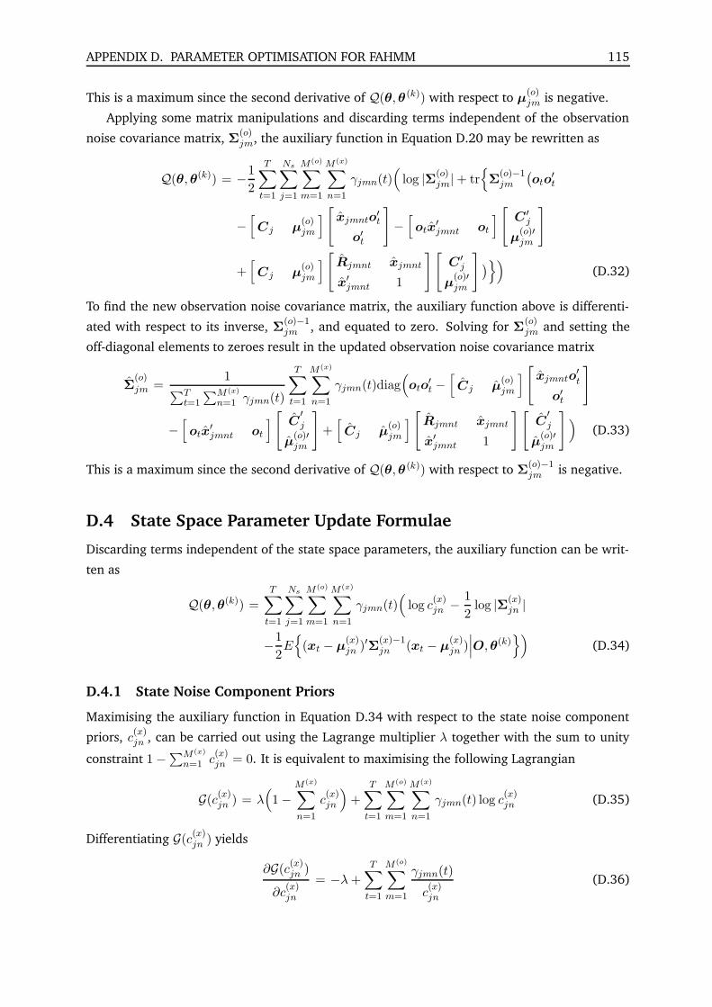
APPENDIX D. PARAMETER OPTIMISATION FOR FAHMM 115
This is a maximum since the second derivative of Q(θ,θ (k)) with respect to µ(o)jm is negative.
Applying some matrix manipulations and discarding terms independent of the observation
noise covariance matrix, Σ(o)jm, the auxiliary function in Equation D.20 may be rewritten as
Q(θ,θ(k)) = −1
2
T∑
t=1
Ns∑
j=1
M(o)∑
m=1
M(x)∑
n=1
γjmn(t)(
log |Σ(o)jm| + tr
Σ(o)−1jm
(oto
′t
−[
Cj µ(o)jm
][
xjmnto′t
o′t
]
−[
otx′jmnt ot
][
C ′j
µ(o)′jm
]
+[
Cj µ(o)jm
][
Rjmnt xjmnt
x′jmnt 1
][
C ′j
µ(o)′jm
]
))
(D.32)
To find the new observation noise covariance matrix, the auxiliary function above is differenti-
ated with respect to its inverse, Σ(o)−1jm , and equated to zero. Solving for Σ
(o)jm and setting the
off-diagonal elements to zeroes result in the updated observation noise covariance matrix
Σ(o)jm =
1∑T
t=1
∑M(x)
n=1 γjmn(t)
T∑
t=1
M(x)∑
n=1
γjmn(t)diag(
oto′t −
[
Cj µ(o)jm
][
xjmnto′t
o′t
]
−[
otx′jmnt ot
][
C′j
µ(o)′jm
]
+[
Cj µ(o)jm
][
Rjmnt xjmnt
x′jmnt 1
][
C′j
µ(o)′jm
])
(D.33)
This is a maximum since the second derivative of Q(θ,θ (k)) with respect to Σ(o)−1jm is negative.
D.4 State Space Parameter Update Formulae
Discarding terms independent of the state space parameters, the auxiliary function can be writ-
ten as
Q(θ,θ(k)) =
T∑
t=1
Ns∑
j=1
M(o)∑
m=1
M(x)∑
n=1
γjmn(t)(
log c(x)jn −
1
2log |Σ
(x)jn |
−1
2E
(xt − µ(x)jn )′Σ
(x)−1jn (xt − µ
(x)jn )
∣∣∣O,θ(k)
)
(D.34)
D.4.1 State Noise Component Priors
Maximising the auxiliary function in Equation D.34 with respect to the state noise component
priors, c(x)jn , can be carried out using the Lagrange multiplier λ together with the sum to unity
constraint 1 −∑M(x)
n=1 c(x)jn = 0. It is equivalent to maximising the following Lagrangian
G(c(x)jn ) = λ
(
1 −M(x)∑
n=1
c(x)jn
)
+T∑
t=1
M(o)∑
m=1
M(x)∑
n=1
γjmn(t) log c(x)jn (D.35)
Differentiating G(c(x)jn ) yields
∂G(c(x)jn )
∂c(x)jn
= −λ+T∑
t=1
M(o)∑
m=1
γjmn(t)
c(x)jn
(D.36)

APPENDIX D. PARAMETER OPTIMISATION FOR FAHMM 116
Setting the derivative to zero together with the sum to unity constraint forms the following pair
of equations
−λ+T∑
t=1
M(o)∑
m=1
γjmn(t)
c(x)jn
= 0
1 −M(x)∑
n=1
c(x)jn = 0
(D.37)
Solving for c(x)jn , the new state noise component priors can be written as
c(x)jn =
T∑
t=1
M(o)∑
m=1
γjmn(t)
T∑
t=1
γj(t)
(D.38)
This is a maximum of G(c(x)jn ) since its second derivative with respect to c
(x)jn is negative.
D.4.2 State Noise Parameters
Differentiating the auxiliary function in Equation D.34 with respect to the state noise mean
vector, µ(x)jn , yields
∂Q(θ,θ(k))
∂µ(x)jn
= Σ(x)−1jn
T∑
t=1
M(o)∑
m=1
γjmn(t)(xjmnt − µ(x)jn ) (D.39)
Equating this to zero and solving for µ(x)jn result in the updated state noise mean vector
µ(x)jn =
T∑
t=1
M(o)∑
m=1
γjmn(t)xjmnt
T∑
t=1
M(o)∑
m=1
γjmn(t)
(D.40)
This is a maximum since the second derivative of Q(θ,θ (k)) with respect to µ(x)jn is negative.
To find the new state noise covariance matrix, the auxiliary function is differentiated with
respect to its inverse, Σ(x)−1jn , as follows
∂Q(θ,θ(k))
∂Σ(x)−1jn
=1
2
T∑
t=1
M(o)∑
m=1
γjmn(t)(
Σ(x)jn −E
(xt − µ(x)jn )(xt − µ
(x)jn )′
∣∣∣O,θ(k)
)
(D.41)
Equating this to zero, solving for Σ(x)jn and setting the off-diagonal elements to zeroes result in
the updated state noise covariance matrix
Σ(x)jn = diag
(
T∑
t=1
M(o)∑
m=1
γjmn(t)(Rjmnt − xjmntµ
(x)′jn − µ
(x)jn x′
jmnt + µ(x)jn µ
(x)′jn
)
T∑
t=1
M(o)∑
m=1
γjmn(t)
)
(D.42)

APPENDIX D. PARAMETER OPTIMISATION FOR FAHMM 117
This is a maximum since the second derivative of Q(θ,θ (k)) with respect to Σ(x)−1jn is negative.
E
Kalman Filtering, Smoothing and Information Forms
Inference algorithms for a linear dynamical system (LDS) with time varying parameters are
presented in this appendix. In contrast with the classical derivations, all the mean vectors are
included to allow extensions to Gaussian mixture models. In the first two sections, Kalman
filtering and smoothing algorithms in the standard covariance form are derived following a
generic forward-backward algorithm. The information form algorithms are derived in Sections
E.3 and E.4. The covariance form filters have to be run sequentially, since the smoother estimates
are based on the filter estimates. The information filters can be run independently and the
smoothed estimates can be obtained by combining the estimates from the forward and backward
passes. This two filter approach to smoothing is presented in the last section.
For quick reference, the conditional distributions in the standard LDS with time-varying pa-
rameters can be written as
p(xt|xt−1) = N (xt;Atxt−1 + µ(x)t ,Σ
(x)t ) (E.1)
p(ot|xt) = N (ot;Ctxt + µ(o)t ,Σ
(o)t ) (E.2)
E.1 Kalman Filter
The derivation follows a so called generic scaled forward-backward algorithm [89]. Let the
forward variable, αxt , be defined as follows
αxt = p(xt,o1:t) = p(o1:t)p(xt|o1:t) =( t∏
τ=1
κτ
)
αxt (E.3)
where κt = p(ot|o1:t−1) are the scaling factors and αxt = p(xt|o1:t) are the scaled forward
variables. Both, the scaling factors and forward variables, are Gaussian distributed due to the
linear Gaussian model assumption. Let xt|τ denoteExt|o1:τ and Σt|τ denoteE(xt−xt|τ )(xt−
xt|τ )′|o1:τ then the scaled forward variable is distributed as
αxt = N (xt;xt|t,Σt|t) (E.4)
118

APPENDIX E. KALMAN FILTERING, SMOOTHING AND INFORMATION FORMS 119
Using the first-order Markov property and the state conditional independence of the obser-
vations in Equations E.1 and E.2, the forward variable, αxt , can be rewritten in the following
recursive form
( t∏
τ=1
κτ
)
αxt = p(xt,o1:t) = p(ot|xt)p(xt,o1:t−1) (E.5)
= p(ot|xt)
∫
p(xt,xt−1 = z,o1:t−1)dz (E.6)
= p(ot|xt)
∫
p(xt|xt−1 = z)p(xt−1 = z,o1:t−1)dz (E.7)
= p(ot|xt)
∫
p(xt|xt−1 = z)( t−1∏
τ=1
κτ
)
αxt−1|zdz (E.8)
κtαxt = p(ot|xt)
∫
p(xt|xt−1 = z)αxt−1|zdz (E.9)
where αxt−1|z = N (z;xt−1|t−1,Σt−1|t−1). The recursion starts off with the initial value αx1 =
p(x1|o1). All the terms in Equation E.9 can be expressed using Gaussians as follows
κtαxt = N (ot;Ctxt + µ(o)t ,Σ
(o)t )
×
∫
N (xt;Atz + µ(x)t ,Σ
(x)t )N (z;xt−1|t−1,Σt−1|t−1)dz (E.10)
where both terms inside the integral are also jointly Gaussian as follows
p(z,xt) =
N(
[
z
xt
]
;
[
xt−1|t−1
Atxt−1|t−1 + µ(x)t
]
,
[
Σt−1|t−1 Σt−1|t−1A′t
AtΣt−1|t−1 AtΣt−1|t−1A′t + Σ
(x)t
])
(E.11)
and since the integration is carried out with respect to z the term on the right hand side reduces
to the probability of xt. Defining xt|t−1 = Atxt−1|t−1 + µ(x)t and Σt|t−1 = AtΣt−1|t−1A
′t + Σ
(x)t ,
Equation E.10 becomes
κtαxt = N (ot;Ctxt + µ(o)t ,Σ
(o)t )N (xt;xt|t−1,Σt|t−1)
= p(ot|xt,o1:t−1)p(xt|o1:t−1) (E.12)
which is not yet in the required form, but can be transformed into it by using Bayes’ formula as
follows
p(ot|xt,o1:t−1)p(xt|o1:t−1) = p(ot|o1:t−1)p(xt|o1:t) (E.13)
and noticing that ot and xt are also jointly Gaussian with the following parameters
p(ot,xt) =
N(
[
xt
ot
]
;
[
xt|t−1
Ctxt|t−1 + µ(o)t
]
,
[
Σt|t−1 Σt|t−1C′t
CtΣt|t−1 CtΣt|t−1C′t + Σ
(o)t
])
(E.14)

APPENDIX E. KALMAN FILTERING, SMOOTHING AND INFORMATION FORMS 120
The form on the right hand side in Equation E.13 can be easily obtained by applying the
conditioning of two multivariate Gaussians in Equation B.14. Therefore, Equation E.12 becomes
κtαxt = N (ot;Ctxt|t−1 + µ(o)t ,CtΣt|t−1C
′t + Σ
(o)t )
×N(xt;xt|t−1 + Kt(ot − Ctxt|t−1 − µ
(o)t ),Σt|t−1 − KtCtΣt|t−1
)(E.15)
where K t = Σt|t−1C′t(CtΣt|t−1C
′t + Σ
(o)t )−1 and which is now the product of the probability
of the current observation given the history up to the time instant t− 1 and the scaled forward
variable as defined earlier.
E.2 Kalman Smoother
The backward variable is defined as usual
βxt = p(ot+1:T |xt) = p(ot+1:T |o1:t)p(ot+1:T |xt)
p(ot+1:T |o1:t)=
( T∏
τ=t+1
κτ
)
βxt (E.16)
where κt = p(ot|o1:t−1) are the same scaling factors as the ones used with the forward vari-
ables. Using again the first-order Markov property and the state conditional independence of
the observations, the backward variable, βxt−1 , can be rewritten in the following recursive form
( T∏
τ=t
κτ
)
βxt−1 =
∫
p(xt = z,ot:T |xt−1)dz (E.17)
=
∫
p(xt = z|xt−1)p(ot|xt = z)p(ot+1:T |xt = z)dz (E.18)
=
∫
p(xt = z|xt−1)p(ot|xt = z)( T∏
τ=t+1
κτ
)
βxt|zdz (E.19)
βxt−1 =1
κt
∫
p(xt = z|xt−1)p(ot|xt = z)βxt|zdz (E.20)
The Kalman smoother estimates, xt and Σt, are the mean vector and covariance matrix of the
state vector, xt, given the entire observation sequence, O. Therefore, they can be represented as
the product of the scaled forward and backward variables as follows
αxt βxt = p(xt|o1:t)p(ot+1:T |xt)
p(ot+1:T |o1:t)= p(xt|O) = N (xt; xt, Σt) (E.21)
The backward recursion can be derived by substituting E.1, E.2, E.4, E.12, E.20 and E.21 into
the product of the scaled forward and backward variables, and doing some algebra as follows
αxt βxt = N (xt;xt|t,Σt|t)
∫
N (z;At+1xt + µ(x)t+1,Σ
(x)t+1)
×N (ot+1;Ct+1z + µ(o)t+1,Σ
(o)t+1)
N (z; xt+1, Σt+1)
κt+1αxt+1|zdz (E.22)
=
∫
N(xt;xt|t + J t(z − At+1xt|t − µ
(x)t+1),Σt|t − J tAt+1Σt|t
)
×N (z; xt+1, Σt+1)dz (E.23)
= N(xt;xt|t + J t(xt+1 − xt+1|t),Σt|t + J t(Σt+1 −Σt+1|t)J
′t
)(E.24)

APPENDIX E. KALMAN FILTERING, SMOOTHING AND INFORMATION FORMS 121
where J t = Σt|tA′t+1Σ
−1t+1|t and Kalman smoother recursions result obviously.
The cross covariance of two consecutive state vectors is also required. It can be obtained by
the scaled forward and backward variables as follows
p(xt−1,xt|O) =1
κtαxt−1p(xt|xt−1)p(ot|xt)βxt (E.25)
Since the current state and the previous state are jointly Gaussian it is easy to obtain their cross
covariance matrix Σt−1,t = ΣtJ′t−1.
E.3 Forward Information Filter
An alternative derivation of the Kalman filter using the information form is presented here.
The derivation requires a backward LDS to be introduced. Assuming invertible state evolution
matrices, the backward LDS can be written as
xt−1 = A−1t xt − A−1
t wt (E.26)
ot = Ctxt + vt (E.27)
where the state evolution noise wt and vt are the same independent noise variables as in the
standard LDS. The observations from time 1 to t, o1:t, can be expressed in terms of xt and xt+1
as
o1:t = C(b)t|t xt + v
(b)t|t (E.28)
o1:t = C(b)t+1|txt+1 + v
(b)t+1|t (E.29)
where the observation matrices, C(b)t|t and C
(b)t+1|t, are constructed as follows
C(b)t|t =
[
C(b)t|t−1
Ct
]
(E.30)
C(b)t+1|t = C
(b)t|t A
−1t+1 (E.31)
with the initial condition C(b)1|1 = C1, and the observation noises, v
(b)t|t and v
(b)t+1|t, are constructed
as follows
v(b)t|t =
[
v(b)t|t−1
vt
]
(E.32)
v(b)t+1|t = v
(b)t|t − C
(b)t|t A
−1t+1wt+1 (E.33)

APPENDIX E. KALMAN FILTERING, SMOOTHING AND INFORMATION FORMS 122
with the initial condition v(b)1|1 = v1. Since the observation and state evolution noises, vt and wt,
are assumed independent, the statistics of v(b)t|t and v
(b)t+1|t can be expressed as
µ(b)t|t =
[
µ(b)t|t−1
µ(o)t
]
(E.34)
Σ(b)t|t =
[
Σ(b)t|t−1 0
0 Σ(o)t
]
(E.35)
µ(b)t+1|t = µ
(b)t|t − C
(b)t|t A
−1t+1µ
(x)t+1 (E.36)
Σ(b)t+1|t = C
(b)t|t A
−1t+1Σ
(x)t+1(A
−1t+1)
′C(b)′t|t + Σ
(b)t|t (E.37)
with the initial conditions µ(b)1|1 = µ
(o)1 and Σ
(b)1|1 = Σ
(o)1 .
The Fisher estimators [66] of xt and xt+1 given the observation sequence o1:t define the
recursions for the forward information filter and predictor covariance matrices, Σ−1t|t and Σ
−1t+1|t,
as follows
Σ−1t|t = C
(b)′t|t Σ
(b)−1t|t C
(b)t|t
= C ′tΣ
(o)−1t Ct + Σ
−1t|t−1 (E.38)
Σ−1t+1|t = C
(b)′t+1|tΣ
(b)−1t+1|t C
(b)t+1|t
= (A−1t+1)
′C(b)′t|t
(C
(b)t|t A
−1t+1Σ
(x)t+1(A
−1t+1)
′C(b)′t|t + Σ
(b)t|t
)−1C
(b)t|t A
−1t+1
= Σ(x)−1t+1 −Σ
(x)−1t+1
((A−1
t+1)′C
(b)′t|t Σ
(b)−1t|t C
(b)t|t A
−1t+1 + Σ
(x)−1t+1
)−1Σ
(x)−1t+1
= Σ(x)−1t+1 −Σ
(x)−1t+1 At+1
(A′t+1Σ
(x)−1t+1 At+1 + Σ
−1t|t
)−1A′t+1Σ
(x)−1t+1 (E.39)
with the initial condition Σ−11|0 = Σ
(i)−11 . The matrix inversion lemma in Equation B.1 is used
between the second and third line in Equation E.39. The forward information filter and the
predictor mean vectors are
Σ−1t|t xt|t = C
(b)′t|t Σ
(b)−1t|t (o1:t − µ
(b)t|t )
= Σ−1t|t−1xt|t−1 + C ′
tΣ(o)−1t (ot − µ
(o)t ) (E.40)
Σ−1t+1|txt+1|t = C
(b)′t+1|tΣ
(b)−1t+1|t (o1:t − µ
(b)t+1|t)
= (A−1t+1)
′C(b)′t|t
(C
(b)t|t
A−1t+1Σ
(x)t+1(A
−1t+1)
′C(b)′t|t
+ Σ(b)t|t
)−1(o1:t + C
(b)t|t
A−1t+1µ
(x)t+1 − µ
(o)t )
= Σ(x)−1t+1 At+1
(A′t+1Σ
(x)−1t+1 At+1 + Σ
−1t|t
)−1C
(b)′t|t Σ
(b)−1t|t (o1:t + C
(b)t|t A
−1t+1µ
(x)t+1 − µ
(o)t )
= Σ(x)−1t+1 At+1
(A′t+1Σ
(x)−1t+1 At+1 + Σ
−1t|t
)−1Σ
−1t|t xt|t + Σ
−1t+1|tµ
(x)t+1 (E.41)
with the initial condition Σ−11|0x1|0 = Σ
(i)−11 µ
(i)1 . The matrix identity in Equation B.2 is used
between the second and third line in Equation E.41.
The information form of the Kalman filter can also be derived by applying the matrix inver-
sion lemma in Equation B.1 to the covariance form recursion. Analogously, the covariance form
of the Kalman filter can be derived from the information form provided above.

APPENDIX E. KALMAN FILTERING, SMOOTHING AND INFORMATION FORMS 123
E.4 Backward Information Filter
The derivation of the backward information filter follows the same method as for the forward
information filter reviewed above. The observations from time t to time T , ot:T , can be expressed
in terms of xt and xt−1 as
ot:T = C(f)t|t xt + v
(f)t|t (E.42)
ot:T = C(f)t−1|txt−1 + v
(f)t−1|t (E.43)
where the observation matrices, C(f)t|t and C
(f)t−1|t, are constructed as follows
C(f)t|t =
[
Ct
C(f)t|t+1
]
(E.44)
C(f)t−1|t = C
(f)t|t At (E.45)
with the initial condition C(f)T |T = CT , and the observation noises, v
(f)t|t and v
(f)t−1|t, are con-
structed as follows
v(f)t|t =
[
vt
v(f)t|t+1
]
(E.46)
v(f)t−1|t = C
(f)t|t wt + v
(f)t|t (E.47)
with the initial condition v(f)T |T = vT . Since the observation and state evolution noises, vt and
wt, are assumed to be independent, the statistics of v(f)t|t and v
(f)t−1|t can be expressed as
µ(f)t|t =
[
µ(o)t
µ(f)t|t+1
]
(E.48)
Σ(f)t|t =
[
Σ(o)t 0
0 Σ(f)t|t+1
]
(E.49)
µ(f)t−1|t = C
(f)t|t µ
(x)t + µ
(f)t|t (E.50)
Σ(f)t−1|t = C
(f)t|t Σ
(x)t C
(f)′t|t + Σ
(f)t|t (E.51)
with initial conditions µ(f)T |T = µ
(o)T and Σ
(f)T |T = Σ
(o)T .
The Fisher estimators [66] of xt and xt−1 given the observation sequence ot:T define the re-
cursions for the backward information filter and predictor covariance matrices, P −1t|t and P−1
t−1|t,
[87] as follows
P−1t|t = C
(f)′t|t Σ
(f)−1t|t C
(f)t|t
= C ′tΣ
(o)−1t Ct + P−1
t|t+1 (E.52)
P−1t−1|t = C
(f)′t−1|tΣ
(f)−1t−1|t C
(f)t−1|t
= A′tC
(f)′t|t
(C
(f)t|t Σ
(x)t C
(f)′t|t + Σ
(f)t|t
)−1C
(f)t|t At
= A′tΣ
(x)−1t
(C
(f)′t|t Σ
(f)−1t|t C
(f)t|t + Σ
(x)−1t
)−1C
(f)′t|t Σ
(f)−1t|t C
(f)t|t At
= A′t
(P−1t|t
Σ(x)t + I
)−1P−1t|t
At (E.53)

APPENDIX E. KALMAN FILTERING, SMOOTHING AND INFORMATION FORMS 124
with the initial condition P −1T |T+1 = 0. The matrix identity in Equation B.2 is used between the
second and third line in Equation E.53. The backward information filter and predictor mean
vectors are
P−1t|t mt|t = C
(f)′t|t Σ
(f)−1t|t (ot:T − µ
(f)t|t )
= P−1t|t+1mt|t+1 + C ′
tΣ(o)−1t (ot − µ
(o)t ) (E.54)
P−1t−1|tmt−1|t = C
(f)′t−1|tΣ
(f)−1t−1|t (ot:T − µ
(f)t−1|t)
= A′tC
(f)′t|t
(C
(f)t|t Σ
(x)t C
(f)′t|t + Σ
(f)t|t
)−1(ot:T − C
(f)t|t µ
(x)t − µ
(f)t|t )
= A′tΣ
(x)−1t
(C
(f)′t|t Σ
(f)−1t|t C
(f)t|t + Σ
(x)−1t
)−1C
(f)′t|t Σ
(f)−1t|t (ot:T − C
(f)t|t µ
(x)t − µ
(f)t|t )
= A′t
(P−1t|t Σ
(x)t + I
)−1P−1t|t (mt|t − µ
(x)t ) (E.55)
with the initial condition P −1T |T+1mT |T+1 = 0.
E.5 Two Filter Formulae for Kalman Smoothing
Sometimes it is beneficial to estimate the smoothed statistics in two independent sweeps. Since
a covariance form of backward Kalman filter in general would require knowledge of the state
noise statistics from time 1 to t [66], the information form has to be used for the backward
sweep. In terms of the current state vector, xt, the observation sequence, O, can be factored as
follows[
o1:t−1
ot:T
]
︸ ︷︷ ︸
O
=
[
C(b)t|t−1
C(f)t|t
]
︸ ︷︷ ︸
C(s)t
xt +
[
v(b)t|t−1
v(f)t|t
]
︸ ︷︷ ︸
v(s)t
(E.56)
where the parameters C(b)t|t−1, v
(b)t|t−1, C
(f)t|t and v
(f)t|t are defined as in Appendices E.3 and E.4.
It should be noted that the observation noises v(b)t|t−1 and v
(f)t|t are independent. The Fisher
estimator [66] of the state vector, xt, given the observation sequence, O, can be expressed in
terms of the parameters C(s)t and Σ
(s)t as follows
Σ−1t = C
(s)′t Σ
(s)−1t C
(s)t
= C(b)′t|t−1Σ
(b)−1t|t−1 C
(b)t|t−1 + C
(f)′t|t Σ
(f)−1t|t C
(f)t|t
= Σ−1t|t−1 + P−1
t|t (E.57)
Σ−1t xt = C
(s)′t Σ
(s)−1t (O − µ
(s)t )
= C(b)′t|t−1Σ
(b)−1t|t−1 (o1:t−1 − µ
(b)t|t−1) + C
(f)′t|t Σ
(f)−1t|t (ot:T − µ
(f)t|t )
= Σ−1t|t−1xt|t−1 + P−1
t|t mt|t (E.58)
The smoothed statistics can be expressed as
Σt = (Σ−1t|t−1 + P−1
t|t )−1 (E.59)
xt = Σt(Σ−1t|t−1
xt|t−1 + P−1t|t
mt|t) (E.60)

APPENDIX E. KALMAN FILTERING, SMOOTHING AND INFORMATION FORMS 125
Similarly, the smoothed statistics can be obtained using the forward filtered estimates, Σt|t, and
backward predicted estimates, P t|t+1, as follows
Σt = (Σ−1t|t + P−1
t|t+1)−1 (E.61)
xt = Σt(Σ−1t|t xt|t + P−1
t|t+1mt|t+1) (E.62)
The equivalence of the RTS and the two filter smoother can be verified using the principle of
mathematical induction. Initially, it holds for the covariance matrix that
ΣT = ΣT |T = (Σ−1T |T + P−1
T |T+1)−1 (E.63)
because P−1T |T+1
= 0. Assuming that Σt+1 = (Σ−1t+1|t
+ P−1t+1|t+1
)−1 holds, the RTS smoother
covariances can be converted into the two filter smoother covariances as follows
Σt = Σt|t + Σt|tA′t+1Σ
−1t+1|t
(Σt+1 −Σt+1|t
)Σ
−1t+1|tAt+1Σt|t
= Σt|t + Σt|tA′t+1Σ
−1t+1|t
((Σ−1
t+1|t+ P−1
t+1|t+1)−1 −Σt+1|t
)Σ
−1t+1|t
At+1Σt|t
= Σt|t + Σt|tA′t+1
((Σt+1|t + Σt+1|tP
−1t+1|t+1Σt+1|t)
−1 −Σ−1t+1|t
)At+1Σt|t
= Σt|t −Σt|tA′t+1
(Σt+1|t + P t+1|t+1
)−1At+1Σt|t
= Σt|t −Σt|t
(Σt|t + P t|t+1
)−1Σt|t
=(Σ
−1t|t + P−1
t|t+1
)−1(E.64)
where the matrix inversion lemma in Equation B.1 is used between the third and fourth line,
and between the fifth and sixth line. Also, the identities Σt+1|t = At+1Σt|tA′t+1 + Σ
(x)t+1 and
P t+1|t+1 = At+1P t|t+1A′t+1 −Σ
(x)t+1 are used between lines four and five.
The RTS smoother mean vectors can be converted into their two filter equivalents in the
same fashion. Initially, it holds that
xT = xT |T = ΣT |T (Σ−1T |T
xT |T + P−1T |T+1
mT |T+1) (E.65)
because P−1T |T+1mT |T+1 = 0. Assuming xt+1 = Σt+1(Σ
−1t+1|txt+1|t+P−1
t+1|t+1mt+1|t+1) holds and
knowing that Σt+1 = (Σ−1t+1|t + P−1
t+1|t+1)−1, the RTS smoother mean vectors can be written as
xt = xt|t + Σt|tA′t+1Σ
−1t+1|t(xt+1 − xt+1|t)
= xt|t + Σt|tA′t+1Σ
−1t+1|t
(Σt+1(Σ
−1t+1|txt+1|t + P−1
t+1|t+1mt+1|t+1) − xt+1|t
)
= xt|t + Σt|tA′t+1Σ
−1t+1|t
((Σ−1
t+1|t + P−1t+1|t+1)
−1(Σ−1t+1|txt+1|t + P−1
t+1|t+1mt+1|t+1) − xt+1|t
)
= xt|t + Σt|tA′t+1
(Σt+1|t + P t+1|t+1
)−1(mt+1|t+1 − xt+1|t)
= xt|t + Σt|t
(Σt|t + P t|t+1
)−1(mt|t+1 − xt|t)
= Σt
(Σ
−1t|t xt|t + P−1
t|t+1mt|t+1
)(E.66)
where the identities xt+1|t = At+1xt|t + µ(x)t+1 and mt+1|t+1 = At+1mt|t+1 + µ
(x)t+1 are used be-
tween the fourth and fifth lines. All the other matrix manipulations are similar to the covariance
derivations described above.

F
Parameter Optimisation for LDS
The parameter update formulae for a standard linear dynamical system (LDS) are derived in this
appendix. The sufficient statistics, xt, Rt and Rt−1,t, for the update formulae may be obtained
using one of the smoothing algorithms presented in Appendix E. The statistics are evaluated
using the set of parameters, θ(k) = C,µ(o),Σ(o),A,µ(x),Σ(x),µ(i),Σ(i), from the previous
iteration in common with the expectation step of the EM algorithm. In the maximisation step, a
set of parameters that maximises the auxiliary function is found
θ = arg maxθ
Q(θ,θ(k)) (F.1)
These parameters will be used as the set of old parameters in the following iteration, θ → θ(k+1).
The following three sections describe the derivation of the parameter update formulae for the
observation space, state space and initial state distribution parameters, respectively.
F.1 Observation Space Parameter Update Formulae
Discarding terms independent of the observation space parameters, the auxiliary function can
be written as
Q(θ,θ(k)) = −1
2
T∑
t=1
(
log |Σ(o)| +E
(ot − Cxt − µ(o))′Σ(o)−1(ot − Cxt − µ(o))∣∣∣O,θ(k)
)
= −1
2
T∑
t=1
(
log |Σ(o)| + tr
Σ(o)−1
(oto
′t −
[
C µ(o)][
xto′t
o′t
]
−[
otx′t ot
][
C ′
µ(o)′
]
+[
C µ(o)][
Rt xt
x′t 1
][
C ′
µ(o)′
]
))
(F.2)
Differentiating the auxiliary function in Equation F.2 with respect to[
C µ(o)]
yields
∂Q(θ,θ(k))
∂[
C µ(o)] =
T∑
t=1
( [
otx′t ot
]
−[
C µ(o)][
Rt xt
x′t 1
])
(F.3)
126

APPENDIX F. PARAMETER OPTIMISATION FOR LDS 127
Equating this to zero and solving for[
C µ(o)]
result in the parameter update
[
C µ(o)]
=( T∑
t=1
[
otx′t ot
] )( T∑
t=1
[
Rt xt
x′t 1
])−1
(F.4)
This is a maximum since the second derivative of Q(θ,θ (k)) with respect to[
C µ(o)]
is negative.
Using the inversion formula for a partitioned matrix in Equation B.6, the individual parameter
update formulae can be written as
C =( T∑
t=1
otx′t −
1
T
T∑
t=1
ot
T∑
t=1
x′t
)( T∑
t=1
Rt −1
T
T∑
t=1
xt
T∑
t=1
x′t
)−1(F.5)
µ(o) =1
T
T∑
t=1
(ot − Cxt
)(F.6)
To find the new observation noise covariance matrix, the auxiliary function in Equation F.2
is differentiated with respect to its inverse, Σ(o)−1, as follows
∂Q(θ,θ(k))
∂Σ(o)−1=
1
2
T∑
t=1
(
Σ(o) − oto
′t +
[
otx′t ot
][
C ′
µ(o)′
]
+[
C µ(o)][
xto′t
o′t
]
−[
C µ(o)][
Rt xt
x′t 1
] [
C ′
µ(o)′
])
(F.7)
Equating this to zero and substituting Equation F.4 into the left hand side of the last term in
Equation F.7, the new observation noise covariance matrix can be written as
Σ(o)
=1
T
T∑
t=1
(
oto′t −
[
C µ(o)][
xto′t
o′t
])
(F.8)
This is a maximum since the second derivative of Q(θ,θ (k)) with respect to Σ(o)−1 is negative.
F.2 State Space Parameter Update Formulae
Discarding terms independent of the state space parameters, the auxiliary function can be writ-
ten as
Q(θ,θ(k)) = −1
2
T∑
t=2
(
log |Σ(x)| +E
(xt − Axt−1 − µ(x))′Σ(x)−1(xt − Axt−1 − µ(x))∣∣∣O,θ(k)
)
= −1
2
T∑
t=2
(
log |Σ(x)| + tr
Σ(x)−1
(Rt −
[
A µ(x)][
R′t−1,t
x′t
]
−[
Rt−1,t xt
][
A′
µ(x)′
]
+[
A µ(x)][
Rt−1 xt−1
x′t−1 1
][
A′
µ(x)′
]
))
(F.9)
Differentiating the auxiliary function in Equation F.9 with respect to[
A µ(x)]
yields
∂Q(θ,θ(k))
∂[
A µ(x)] =
T∑
t=2
( [
Rt−1,t xt
]
−[
A µ(x)][
Rt−1 xt−1
x′t−1 1
])
(F.10)

APPENDIX F. PARAMETER OPTIMISATION FOR LDS 128
Equating this to zero and solving for[
A µ(x)]
result in the updated parameters
[
A µ(x)]
=( T∑
t=2
[
Rt−1,t xt
] )( T∑
t=2
[
Rt−1 xt−1
x′t−1 1
])−1
(F.11)
This is a maximum since the second derivative of Q(θ,θ(k)) with respect to[
A µ(x)]
is negative.
Using the inversion formula for a partitioned matrix in Equation B.6, the individual parameter
update formulae can be written as
A =( T∑
t=2
Rt−1,t −1
T − 1
T∑
t=2
xt
T∑
t=2
x′t−1
)( T∑
t=2
Rt−1 −1
T − 1
T∑
t=2
xt−1
T∑
t=2
x′t−1
)−1(F.12)
µ(x) =1
T − 1
T∑
t=2
(xt − Axt−1
)(F.13)
To find the new state noise covariance matrix, the auxiliary function in Equation F.9 is differ-
entiated with respect to its inverse, Σ(x)−1, as follows
∂Q(θ,θ(k))
∂Σ(x)−1=
1
2
T∑
t=2
(
Σ(x) − R
′t +
[
Rt−1,t xt
][
A′
µ(x)′
]
+[
A µ(x)][
R′t−1,t
x′t
]
−[
A µ(x)][
Rt−1 xt−1
x′t−1 1
][
A′
µ(x)′
])
(F.14)
Equating this to zero and substituting Equation F.11 into the left hand side of the last term in
Equation F.14, the new state noise covariance matrix can be written as
Σ(x)
=1
T − 1
T∑
t=2
(
Rt −[
A µ(x)] [
Rt−1,t xt
]′ )
(F.15)
This is a maximum since the second derivative of Q(θ,θ (k)) with respect to Σ(x)−1 is negative.
F.3 Initial State Distribution Parameter Update Formulae
Discarding terms independent of the initial state noise distribution parameters, the auxiliary
function can be written as
Q(θ,θ(k)) = −1
2
(
log |Σ(i)| +E
(x1 − µ(i))′Σ(i)−1(x1 − µ(i))∣∣∣O,θ(k)
)
= −1
2
(
log |Σ(i)| + tr
Σ(i)−1
(R1 − µ(i)x′
1 − x1µ(i)′ + µ(i)µ(i)′
))
(F.16)
Differentiating the auxiliary function in Equation F.16 with respect to the initial state noise
mean vector, µ(i), yields
∂Q(θ,θ(k))
∂µ(i)= Σ
(i)−1(x1 − µ(i)) (F.17)

APPENDIX F. PARAMETER OPTIMISATION FOR LDS 129
Equating this to zero and solving for µ(i) result in the initial state noise mean vector update
µ(i) = x1 (F.18)
This is a maximum since the second derivative of Q(θ,θ (k)) with respect to µ(i) is negative.
To find the new initial state noise covariance matrix, the auxiliary function is differentiated
with respect to its inverse, Σ(i)−1, as follows
∂Q(θ,θ(k))
∂Σ(i)−1=
1
2
(
Σ(i) − R1 + µ(i)x′
1 + x1µ(i)′ − µ(i)µ(i)′
)
(F.19)
Equating this to zero and solving for Σ(i) result in the initial state noise covariance matrix update
Σ(i)
= R1 − µ(i)µ(i)′ (F.20)
This is a maximum since the second derivative of Q(θ,θ (k)) with respect to Σ(i)−1 is negative.

G
Gibbs Sampling for SLDS
An approximate inference scheme for the switching linear dynamical system (SLDS) based on
Gibbs sampling is derived in this appendix. In common with standard Monte Carlo sampling
algorithms, the proposal distribution has to be carefully designed. The efficiency of Monte Carlo
methods depends on the size of the state space the samples are drawn from. Due to the tractable
substructures in SLDS, Rao-Blackwellisation may be employed to increase efficiency. For the
SLDS, samples are drawn from the discrete state space and the continuous state space statistics
may be obtained holding the estimated discrete state sequence fixed. The proposal distribution
to draw the discrete states for a time instant is derived in the following section.
G.1 Proposal Distribution
The proposal distribution used in Rao-Blackwellised Gibbs sampling for switching linear dynam-
ical systems can be expressed as [26]
P (qt|O, q(n)−t ) ∝
P (q(n−1)t+1 |qt)P (qt|q
(n)t−1)p(ot|o1:t−1, q
(n)1:t )
∫
p(ot+1:T |xt, q(n−1)t+1:T )p(xt|o1:t, q
(n)1:t )dxt (G.1)
Using the parameters C(f)t|t+1, µ
(f)t|t+1 and Σ
(f)t|t+1 for the likelihood p(ot+1:T |xt, q
(n−1)t+1:T ) as defined
in Appendix E.4, the above integral can be written as
∫
p(ot+1:T |xt, q(n−1)t+1:T )p(xt|o1:t, q
(n)1:t )dxt =
∫
N (ot+1:T ;C(f)t|t+1xt + µ
(f)t|t+1,Σ
(f)t|t+1)N (xt;xt|t,Σt|t)dxt
= N (ot+1:T ;C(f)t|t+1xt|t + µ
(f)t|t+1,C
(f)t|t+1Σt|tC
(f)′t|t+1 + Σ
(f)t|t+1) (G.2)
Using the backward information filter variables from Appendix E.4 and the identity for determi-
nants in Equation B.3, the determinant of the covariance matrix for the above Gaussian can be
130

APPENDIX G. GIBBS SAMPLING FOR SLDS 131
expressed as
∣∣C
(f)t|t+1Σt|tC
(f)′t|t+1 + Σ
(f)t|t+1
∣∣ =
∣∣Σ
(f)t|t+1
∣∣∣∣Σt|t
∣∣∣∣C
(f)′t|t+1Σ
(f)−1t|t+1 C
(f)t|t+1 + Σ
−1t|t
∣∣
=∣∣Σ
(f)t|t+1
∣∣∣∣Σt|tP
−1t|t+1 + I
∣∣ (G.3)
where∣∣Σ
(f)t|t+1
∣∣ does not depend on qt.
Using the matrix inversion lemma in Equation B.1, the inverse covariance matrix of the
Gaussian in Equation G.2 can be written as
(C(f)t|t+1Σt|tC
(f)′t|t+1 + Σ
(f)t|t+1)
−1 =
Σ(f)−1t|t+1 −Σ
(f)−1t|t+1 C
(f)t|t+1
(C
(f)′t|t+1Σ
(f)−1t|t+1 C
(f)t|t+1 + Σ
−1t|t
)−1C
(f)′t|t+1Σ
(f)−1t|t+1
= Σ(f)−1t|t+1 −Σ
(f)−1t|t+1 C
(f)t|t+1
(P−1t|t+1 + Σ
−1t|t
)−1C
(f)′t|t+1Σ
(f)−1t|t+1 (G.4)
Writing the Gaussian as Z exp(− 12γ) where Z is a constant. The term γ can be expressed as
γ = (ot+1:T − C(f)t|t+1xt|t − µ
(f)t|t+1)
′(Σ
(f)−1t|t+1 −Σ
(f)−1t|t+1 C
(f)t|t+1
(P−1t|t+1 + Σ
−1t|t
)−1C
(f)′t|t+1Σ
(f)−1t|t+1
)
×(ot+1:T − C(f)t|t+1xt|t − µ
(f)t|t+1)
= (ot+1:T − µ(f)t|t+1)
′Σ
(f)−1t|t+1 (ot+1:T − µ
(f)t|t+1) + x′
t|tP−1t|t+1xt|t − 2x′
t|tP−1t|t+1mt|t+1
−(mt|t+1 − xt|t)′P−1
t|t+1
(P−1t|t+1 + Σ
−1t|t
)−1P−1t|t+1(mt|t+1 − xt|t) (G.5)
where (ot+1:T −µ(f)t|t+1)
′Σ
(f)−1t|t+1 (ot+1:T −µ
(f)t|t+1) does not depend on qt. The proposal distribution
results discarding all terms independent of qt
P (qt|O, q(n)−t ) ∝
P (q(n−1)t+1 |qt)P (qt|q
(n)t−1)N (ot;Ctxt|t−1 + µ
(o)t ,CtΣt|t−1C
′t + Σ
(o)t )
∣∣Σt|tP
−1t|t+1 + I
∣∣−
12
× exp
x′t|tP
−1t|t+1mt|t+1 −
1
2x′t|tP
−1t|t+1xt|t
+1
2(mt|t+1 − xt|t)
′P−1t|t+1
(P−1t|t+1 + Σ
−1t|t
)−1P−1t|t+1(mt|t+1 − xt|t)
(G.6)

Bibliography
[1] C. Andrieu, N. de Freitas, A. Doucet, and M.I. Jordan. An introduction to MCMC for
machine learning. Machine Learning, 50(1-2):5–43, 2003.
[2] H. Attias. Independent factor analysis. Neural Computation, 11(4):803–851, 1999.
[3] H. Attias. Inferring parameters and structure of latent variable models by variational
Bayes. In Proceedings UAI, pages 21–30, 1999.
[4] S. Axelrod, R. Gopinath, and P. Olsen. Modeling with a subspace constraint on inverse
covariance matrices. In Proceedings ICSLP, pages 2177–2180, 2002.
[5] M. Bacchiani and M. Ostendorf. Using automatically-derived acoustic subword units in
large vocabulary speech recognition. In Proceedings ICSLP, volume 5, pages 1843–1846,
1998.
[6] L.R. Bahl, P.F. Brown, P.V. de Souza, and R.L. Mercer. Maximum mutual information
estimation of hidden Markov model parameters for speech recognition. In Proceedings
ICASSP, pages 49–52, 1986.
[7] L.R. Bahl, P.V. de Souza, P.S. Gopalkrishnan, D. Nahamoo, and M.A. Picheny. Context
dependent modelling of phones in continuous speech using decision trees. In Proceedings
DARPA Speech and Natural Language Processing Workshop, pages 264–270, 1991.
[8] Y. Bar-Shalom and X-R. Li. Estimation and Tracking: Principles, Techniques and Software.
Artech House, 1993.
[9] L.E. Baum and T. Petrie. Statistical inference for probabilistic functions of finite state
Markov chains. Annals of Mathematical Statistics, 37:1554–1563, 1966.
[10] L.E. Baum, T. Petrie, G. Soules, and N. Weiss. A maximization technique occuring in the
statistical analysis of probabilistic functions of Markov chains. Annals of Mathematical
Statistics, 41(1):164–171, 1970.
132

Bibliography 133
[11] M.J. Beal. Variational Algorithms for Approximate Bayesian Inference. PhD thesis, Univer-
sity of London, 2003.
[12] J.A. Bilmes. A gentle tutorial of the EM algorithm and its application to parameter esti-
mation for Gaussian mixture and hidden Markov models. Technical Report TR-97-021,
Department of Electrical Engineering and Computer Science, University of California,
Berkeley, 1998. Available at http://www.icsi.berkeley.edu/ftp/pub/techreports/.
[13] C. Bishop. Neural Networks for Pattern Recognition. Oxford University Press, 1995.
[14] C.S. Blackburn. Articulatory Methods for Speech Production and Recognition. PhD thesis,
University of Cambridge, 1996.
[15] X. Boyen and D. Koller. Tractable inference for complex stochastic processes. In Proceed-
ings UAI, pages 33–42, 1998.
[16] C.K. Carter and R. Kohn. On Gibbs sampling for state space models. Biometrika, 81:541–
553, 1994.
[17] C.K. Carter and R. Kohn. Markov chain Monte Carlo in conditionally Gaussian state space
models. Biometrika, 83:589–601, 1996.
[18] S.S. Chen and P.S. Gopalakrishnan. Clustering via the Bayesian information criterion with
applications in speech recognition. In Proceedings ICASSP, volume 2, pages 645–648,
1998.
[19] S.B. Davis and P. Mermelstein. Comparison of parametric representations for monosyl-
labic word recognition in continuously spoken sentences. IEEE Transactions on Acoustics
Speech and Signal Processing, 28:357–366, 1980.
[20] J.R. Deller, J.H.L. Hansen, and J.G. Proakis. Discrete-Time Processing of Speech Signals.
Macmillan, 1993.
[21] A.P. Dempster, N.M. Laird, and D.B. Rubin. Maximum likelihood from incomplete data
via the EM algorithm. Journal of the Royal Statistical Society, 39:1–38, 1977.
[22] L. Deng and J. Ma. A statistical coarticulatory model for the hidden vocal-tract-resonance
dynamics. In Proceedings Eurospeech, volume 4, pages 1499–1502, 1999.
[23] S. Dharanipragada and K. Visweswariah. Covariance and precision modeling in shared
multiple subspaces. In Proceedings ICASSP, volume 1, pages 904–907, 2003.
[24] V. Digalakis. Segment-Based Stochastic Models of Spectral Dynamics for Continuous Speech
Recognition. PhD thesis, Boston University, 1992.
[25] V. Digalakis, J.R. Rohlicek, and M. Ostendorf. ML estimation of a stochastic linear system
with the EM algorithm and its application to speech recognition. IEEE Transactions on
Speech and Audio Processing, 1(4):431–442, 1993.

Bibliography 134
[26] A. Doucet and C. Andrieu. Iterative algorithms for state estimation of jump Markov linear
systems. IEEE Transactions on Signal Processing, 49(6):1216–1227, 2001.
[27] A. Doucet, N. de Freitas, and N. Gordon. Sequential Monte Carlo Methods in Practice.
Springer-Verlag, 2001.
[28] A. Doucet, S. Godsill, and C. Andrieu. On sequential Monte Carlo sampling methods for
Bayesian filtering. Statistics and Computing, 10(3):197–208, 2000.
[29] J. Frankel. Linear Dynamic Models for Automatic Speech Recognition. PhD thesis, University
of Edinburgh, 2003.
[30] J. Frankel and S. King. ASR - articulatory speech recognition. In Proceedings Eurospeech,
pages 599–602, 2001.
[31] J. Frankel, K. Richmond, S. King, and P. Taylor. An automatic speech recognition sys-
tem using neural networks and linear dynamic models to recover and model articulatory
traces. In Proceedings ICSLP, volume 4, pages 254–257, 2000.
[32] M.J.F. Gales. The generation and use of regression class trees for MLLR adaptation. Tech-
nical Report CUED/F-INFENG/TR.263, Cambridge University Engineering Department,
1996. Available at http://mi.eng.cam.ac.uk/reports/.
[33] M.J.F. Gales. Maximum likelihood linear transformations for HMM-based speech recog-
nition. Computer Speech and Language, 12(2):75–98, 1998.
[34] M.J.F. Gales. Semi-tied covariance matrices for hidden Markov models. IEEE Transactions
on Speech and Audio Processing, 7(3):272–281, 1999.
[35] M.J.F. Gales. Maximum likelihood multiple subspace projections for hidden Markov mod-
els. IEEE Transactions on Speech and Audio Processing, 10(2):37–47, 2002.
[36] M.J.F. Gales, K.M. Knill, and S.J. Young. State-based Gaussian selection in large vocabu-
lary continuous speech recognition using HMMs. IEEE Transactions on Speech and Audio
Processing, 7(2):152–161, 1999.
[37] M.J.F. Gales and S.J. Young. The theory of segmental hidden Markov models. Technical
Report CUED/F-INFENG/TR.133, Cambridge University Engineering Department, 1993.
Available at http://mi.eng.cam.ac.uk/reports/.
[38] J.L. Gauvain and C.H. Lee. Maximum a-posteriori estimation for multivariate Gaussian
mixture observations of Markov chains. IEEE Transactions on Speech and Audio Processing,
2(2):291–298, 1994.
[39] Z. Ghahramani. Learning dynamic Bayesian networks. In C.L. Giles and M. Gori, editors,
Adaptive Processing of Sequences and Data Structures, volume 1387 of Lecture Notes in
Computer Science, pages 168–197. Springer, 1998.

Bibliography 135
[40] Z. Ghahramani and G. Hinton. The EM algorithm for mixtures of factor analyzers. Techni-
cal Report CRG-TR-96-1, Department of Computer Science, University of Toronto, 1996.
Available at http://www.gatsby.ucl.ac.uk/~zoubin/papers.html.
[41] Z. Ghahramani and G. Hinton. Parameter estimation for linear dynamical systems.
Technical Report CRG-TR-96-2, Department of Computer Science, University of Toronto,
1996. Available at http://www.gatsby.ucl.ac.uk/~zoubin/papers.html.
[42] Z. Ghahramani and G.E. Hinton. Variational learning for switching state-space models.
Neural Computation, 12(4):963–996, 1998.
[43] Z. Ghahramani and M.I. Jordan. Factorial hidden Markov models. Machine Learning,
29(2-3):245–273, 1997.
[44] L. Gillick and S.J. Cox. Some statistical issues in the comparison of speech recognition.
In Proceedings ICASSP, pages 532–535, 1989.
[45] J.J. Godfrey, E.C. Holliman, and J. McDaniel. SWITCHBOARD: Telephone speech corpus
for research and development. In Proceedings ICASSP, volume 1, pages 517–520, 1992.
[46] R.A. Gopinath. Constrained maximum likelihood modeling with Gaussian distributions.
In Proceedings Broadcast News Transcription and Understanding Workshop, 1998.
[47] R.A. Gopinath. Maximum likelihood modeling with Gaussian distributions for classifica-
tion. In Proceedings ICASSP, volume 2, pages 661–664, 1998.
[48] R.A. Gopinath, B. Ramabhadran, and S. Dharanipragada. Factor analysis invariant to
linear transformations of data. In Proceedings ICSLP, pages 397–400, 1998.
[49] T. Hain, P. Woodland, G. Evermann, M. Gales, A. Liu, G. Moore, D. Povey, and L. Wang. Au-
tomatic transcription of conversational telephone speech - development of the CU-HTK
2002 system. Technical Report CUED/F-INFENG/TR.465, Cambridge University Engi-
neering Department, 2003. Available at http://mi.eng.cam.ac.uk/reports/.
[50] T. Hain, P.C. Woodland, G. Evermann, and D. Povey. The CU-HTK March 2000 HUB5E
transcription system. In Proceedings Speech Transcription Workshop, 2000.
[51] T. Hain, P.C. Woodland, T.R. Niesler, and E.W.D. Whittaker. The 1998 HTK system for
transcription of conversational telephone speech. In Proceedings ICASSP, volume 1, pages
57–60, 1999.
[52] D.A. Harville. Matrix Algebra from a Statistician’s Perspective. Springer, 1997.
[53] H. Hermansky. Perceptual linear prediction (PLP) of speech. Journal of the Acoustic Society
of America, 87(4):1738–1752, 1990.

Bibliography 136
[54] T. Heskes and O. Zoeter. Expectation propagation for approximate inference in dynamic
Bayesien networks. In Proceedings UAI, pages 216–223, 2002.
[55] T. Heskes and O. Zoeter. Generalized belief propagation for approximate inference in
hybrid Bayesian networks. In C.M. Bishop and B.J. Frey, editors, Proceedings Artificial
Intelligence & Statistics, 2003.
[56] W.J. Holmes. Modelling Segmental Variability for Automatic Speech Recognition. PhD thesis,
University of London, 1997.
[57] W.J. Holmes and M.J. Russell. Experimental evaluation of segmental HMMs. In Proceed-
ings ICASSP, volume 1, pages 536–539, 1995.
[58] W.J. Holmes and M.J. Russell. Modeling speech variability with segmental HMMs. In
Proceedings ICASSP, volume 1, pages 447–4450, 1996.
[59] W.J. Holmes and M.J. Russell. Linear dynamic segmental HMMs: Variability representa-
tion and training procedure. In Proceedings ICASSP, volume 2, pages 1399–1402, 1997.
[60] W.J. Holmes and M.J. Russell. Probabilistic-trajectory segmental HMMs. Computer Speech
and Language, 13(1):3–37, 1999.
[61] M. Isard and A. Blake. Condensation – conditional density propagation for visual tracking.
International Journal of Computer Vision, 29(1):5–28, 1998.
[62] F. Jelinek. Continuous speech recognition by statistical methods. IEEE Proceedings,
64(4):532–556, 1976.
[63] R.A. Johnson and D.W. Wichern. Applied Multivariate Statistical Analysis. Prentice Hall, 4
edition, 1998.
[64] M.I. Jordan, Z. Ghahramani, T. Jaakkola, and L. K. Saul. An introduction to variational
methods in graphical models. Machine Learning, 37(2):183–233, 1999.
[65] B.H. Juang, W. Chou, and C.H. Lee. Minimum classification error rate methods for speech
recognition. IEEE Transactions on Speech and Audio Processing, 5(3):257–265, 1997.
[66] T. Kailath, A.H. Sayed, and B. Hassibi. Linear Estimation. Prentice Hall, 2000.
[67] R.E. Kalman. A new approach to linear filtering and prediction problems. Transactions
of the American Society of Mechanical Engineering, Series D, Journal of Basic Engineering,
82:35–45, 1960.
[68] R.E. Kalman and R.S. Bucy. New results in linear filtering and prediction theory. Trans-
actions of the American Society of Mechanical Engineering, Series D, Journal of Basic Engi-
neering, 83:95–108, 1961.

Bibliography 137
[69] S. Kapadia. Discriminative Training of Hidden Markov Models. PhD thesis, University of
Cambridge, 1998.
[70] S.M. Katz. Estimation of probabilities from sparse data for the language model compo-
nent of a speech recognizer. IEEE Transactions on Acoustics Speech and Signal Processing,
35(3):400–411, 1987.
[71] O.A. Kimball. Segment Modeling Alternatives for Continuous Speech Recognition. PhD
thesis, Boston University, 1995.
[72] N. Kumar. Investigation of Silicon-Auditory Models and Generalization of Linear Discrim-
inant Analysis for Improved Speech Recognition. PhD thesis, Johns Hopkins University,
1997.
[73] L.F. Lamel, R.H. Kassel, and S. Seneff. Speech database development: Design and anal-
ysis of the acoustic-phonetic corpus. In Proceedings DARPA Speech Recognition Workshop,
pages 100–109, 1986.
[74] S.L. Lauritzen. Propagation of probabilities, means and variances in mixed graphical
association models. Journal of the American Statistical Association, 87:1098–1108, 1992.
[75] L. Lee and R.C. Rose. Speaker normalization using efficient frequency warping proce-
dures. In Proceedings ICASSP, volume 1, pages 353–356, 1996.
[76] L.J. Lee, H. Attias, and L. Deng. Variational inference and learning for segmental switch-
ing state space models of hidden speech dynamics. In Proceedings ICASSP, volume 1,
pages 920–923, 2003.
[77] C.J. Leggetter. Improved Acoustic Modelling for HMMs Using Linear Transformations. PhD
thesis, University of Cambridge, 1995.
[78] C.J. Leggetter and P.C. Woodland. Maximum likelihood linear regression for speaker
adaptation of continuous density HMMs. Computer Speech and Language, 9(2):171–186,
1995.
[79] L.A. Liporace. Maximum likelihood estimation for multivariate observations of Markov
sources. IEEE Transactions on Information Theory, IT-28(5):729–734, 1982.
[80] X. Liu and M.J.F. Gales. Automatic model complexity control using marginalised discrim-
inative growth functions. In Proceedings ASRU, pages 37–42, 2003.
[81] X. Liu, M.J.F. Gales, and P.C. Woodland. Automatic complexity control for HLDA systems.
In Proceedings ICASSP, volume 1, pages 132–135, 2003.
[82] J. Ma and L. Deng. Optimization of dynamic regimes in a statistical hidden dynamic
model for conversational speech recognition. In Proceedings Eurospeech, volume 3, pages
1339–1342, 1999.

Bibliography 138
[83] J. Ma and L. Deng. A path-stack algorithm for optimizing dynamic regimes in a statistical
hidden dynamic model of speech. Computer Speech and Language, 14(2):101–114, 2000.
[84] J. Ma and L. Deng. A mixed-level switching dynamic system for continuous speech recog-
nition. Computer Speech and Language, 18(1):49–65, 2004.
[85] J.Z. Ma and L. Deng. Efficient decoding strategy for conversational speech recognition
using state-space models for vocal-tract-resonance dynamics. In Proceedings Eurospeech,
pages 603–606, 2001.
[86] D.J.C. MacKay. Introduction to Monte Carlo methods. In M.I. Jordan, editor, Learning in
Graphical Models, NATO Science Series, pages 175–204. Kluwer Academic Press, 1998.
[87] D.Q. Mayne. A solution of the smoothing problem for linear dynamic systems. Automat-
ica, 4:73–92, 1966.
[88] D.R.H. Miller and J.W. McDonough. BBN 1997 acoustic modelling. Presented at Conver-
sational Speech Recognition Workshop DARPA Hub-5E Evaluation, May 1997.
[89] T.P. Minka. From hidden Markov models to linear dynamical systems. Technical Re-
port #531, Vision and Modeling Group, MIT Media Laboratory, 1999. Available at
http://vismod.www.media.mit.edu/~tpminka/papers/learning.html.
[90] T.P. Minka. Expectation propagation for approximate Bayesian inference. In Proceedings
UAI, pages 362–369, 2001.
[91] T.P. Minka. A family of algorithms for approximate Bayesian inference. PhD thesis, Mas-
sachusetts Institute of Technology, 2001.
[92] T.P. Minka. Using lower bounds to approximate integrals. Informal notes available at
http://www.stat.cmu.edu/~minka/papers/learning.html, 2001.
[93] K. Murphy. Learning switching Kalman filter models. Technical Re-
port 98-10, Compaq Cambridge Research Lab., 1998. Available at
http://www.ai.mit.edu/~murphyk/publ.html.
[94] K. Murphy. From belief propagation to expectation propagation. Informal notes available
at http://www.ai.mit.edu/~murphyk/papers.html, 2001.
[95] K.P. Murphy. A variational approximation for Bayesian networks with discrete and con-
tinuous latent variables. In Proceedings UAI, pages 457–466, 1999.
[96] K.P. Murphy. Dynamic Bayesian Networks: Representation, Inference and Learning. PhD
thesis, University of California, Berkeley, 2002.
[97] A. Nadas. A decision theoretic formulation of a training problem in speech recognition
and a comparison of training by unconditional versus conditional maximum likelihood.
IEEE Transactions on Acoustics Speech and Signal Processing, 31:814–817, 1983.

Bibliography 139
[98] H.J. Nock, M.J.F. Gales, and S.J. Young. A comparative study of methods for phonetic
decision-tree state clustering. In Proceedings Eurospeech, volume 1, pages 111–114, 1997.
[99] P.A. Olsen and R.A. Gopinath. Modeling inverse covariance matrices by basis expansion.
IEEE Transactions on Speech and Audio Processing, 12(1):37–46, 2004.
[100] M. Ostendorf. Moving beyond the ’beads-on-a-string’ model of speech. In Proceedings
ASRU, volume 1, pages 79–84, 1999.
[101] M. Ostendorf and V. Digalakis. The stochastic segment model for continuous speech recog-
nition. In Proceedings The 25th Asilomar Conference on Signals, Systems and Computers,
pages 964–968, 1991.
[102] M. Ostendorf, V. Digalakis, and O. Kimball. From HMM’s to segment models: A unified
view of stochastic modeling for speech recognition. IEEE Transactions on Speech and Audio
Processing, 4(5):360–378, 1996.
[103] V. Pavlovic, J.M. Rehg, T-J. Cham, and K.P. Murphy. A dynamic Bayesian network approach
to figure tracking using learned dynamic models. In Proceedings ICCV, pages 94–101,
1999.
[104] V. Pavlovic, J.M. Rehg, and J. MacCormick. Learning switching linear models of human
motion. In Proceedings NIPS, pages 981–987, 2000.
[105] J. Picone, S. Pike, R. Regan, T. Kamm, J. Bridle, L. Deng, Z. Ma, H. Richards, and
M. Schuster. Initial evaluation of hidden dynamic models on conversational speech. In
Proceedings ICASSP, volume 1, pages 109–112, 1999.
[106] D. Povey and P.C. Woodland. Minimum phone error and I-smoothing for improved dis-
criminative training. In Proceedings ICASSP, volume 1, pages 105–108, 2002.
[107] P. Price, W.M. Fisher, J. Bernstein, and D.S. Pallett. The DARPA 1000-word Resource Man-
agement database for continuous speech recognition. In Proceedings ICASSP, volume 1,
pages 651–654, 1988.
[108] L.R. Rabiner. A tutorial on hidden Markov models and selected applications in speech
recognition. IEEE Proceedings, 77(2):257–285, 1989.
[109] H.E. Rauch. Solutions to the linear smoothing problem. IEEE Transactions on Automatic
Control, 8:371–372, 1963.
[110] H.E. Rauch, F. Tung, and C.T. Striebel. Maximum likelihood estimates of linear dynamic
systems. American Institute of Aeronautics and Astronautics Journal, 3(8):1445–1450,
1965.
[111] H.B. Richards and J.S. Bridle. The HDM: A segmental hidden dynamic model of coartic-
ulation. In Proceedings ICASSP, volume 1, pages 357–360, 1999.

Bibliography 140
[112] C.P. Robert and G. Casella. Monte Carlo Statistical Methods. Springer-Verlag, 1999.
[113] A-V.I. Rosti and M.J.F. Gales. Generalised linear Gaussian models. Technical Report
CUED/F-INFENG/TR.420, Cambridge University Engineering Department, 2001. Avail-
able at http://mi.eng.cam.ac.uk/reports/.
[114] A-V.I. Rosti and M.J.F. Gales. Factor analysed hidden Markov models. In Proceedings
ICASSP, volume 1, pages 949–952, 2002.
[115] A-V.I. Rosti and M.J.F. Gales. Factor analysed hidden Markov models for speech recog-
nition. Technical Report CUED/F-INFENG/TR.453, Cambridge University Engineering
Department, 2003. Available at http://mi.eng.cam.ac.uk/reports/.
[116] A-V.I. Rosti and M.J.F. Gales. Switching linear dynamical systems for speech recognition.
Technical Report CUED/F-INFENG/TR.461, Cambridge University Engineering Depart-
ment, 2003. Available at http://mi.eng.cam.ac.uk/reports/.
[117] A-V.I. Rosti and M.J.F. Gales. Factor analysed hidden Markov models for speech recogni-
tion. Computer Speech and Language, 18(2):181–200, 2004.
[118] A-V.I. Rosti and M.J.F. Gales. Rao-Blackwellised Gibbs sampling for switching linear dy-
namical systems. In Proceedings ICASSP, 2004.
[119] S. Roweis and Z. Ghahramani. A unifying review of linear Gaussian models. Neural
Computation, 11(2):305–345, 1999.
[120] D.B. Rubin and D.T. Thayer. EM algorithms for ML factor analysis. Psychometrika,
47(1):69–76, 1982.
[121] L. Saul and M.I. Jordan. Exploiting tractable substructures in intractable networks. In
Proceedings NIPS, pages 486–492, 1996.
[122] L. Saul and M. Rahim. Maximum likelihood and minimum classification error factor anal-
ysis for automatic speech recognition. IEEE Transactions on Speech and Audio Processing,
8(2):115–125, 1999.
[123] F. Seide, J-L. Zhou, and L. Deng. Coarticulation modeling by embedding a target-directed
hidden trajectory model into HMM – MAP decoding and evaluation. In Proceedings
ICASSP, volume 1, pages 748–751, 2003.
[124] L.F. Uebel and P.C. Woodland. An investigation into vocal tract length normalisation. In
Proceedings Eurospeech, volume 6, pages 2527–2530, 1999.
[125] A.J. Viterbi. Error bounds for convolutional codes and an asymptotically optimal decoding
algorithm. IEEE Transactions on Information Theory, IT-13:260–269, 1967.

Bibliography 141
[126] G.C.G. Wei and M.A. Tanner. A Monte Carlo implementation of the EM algorithm and the
poor man’s data augmentation algorithms. Journal of the American Statistical Association,
85:699–704, 1990.
[127] E.W. Weisstein. Eric Weisstein’s World of Mathematics. Wolfram Research Inc., 2004.
Available at http://mathworld.wolfram.com/.
[128] P.C. Woodland and D. Povey. Large scale discriminative training of hidden Markov models
for speech recognition. Computer Speech and Language, 16(1):25–47, 2002.
[129] S. Young, D. Kershaw, J. Odell, D. Ollason, V. Valtchev, and P. Woodland. The HTK Book
(for HTK Version 3.0). Cambridge University, 2000.
[130] S.J. Young, J.J. Odell, and P.C. Woodland. Tree based state tying for high accuracy acoustic
modelling. In Proceedings ARPA Human Language Technology Workshop, pages 307–312,
1994.
[131] S.J. Young, N.H. Russell, and J.H.S Thornton. Token passing: a simple conceptual model
for connected speech recognition systems. Technical Report CUED/F-INFENG/TR.38,
Cambridge University Engineering Department, 1989.
[132] R.S. Zemel. A Minimum Description Length Framework for Unsupervised Learning. PhD
thesis, University of Toronto, 1994.
[133] J-L. Zhou, F. Seide, and L. Deng. Coarticulation modeling by embedding a target-directed
hidden trajectory model into HMM – model and training. In Proceedings ICASSP, vol-
ume 1, pages 744–747, 2003.
[134] O. Zoeter and T. Heskes. Hierarchical visualization of time-series data using switching
linear dynamical systems. In Proceedings UAI, pages 1201–1214, 2003.
[135] G.G. Zweig. Speech Recognition with Dynamic Bayesian Networks. PhD thesis, University
of California, Berkeley, 1998.