remote sensing

Article

Deep Learning for SAR Image Despeckling

Francesco Lattari 1,∗, Borja Gonzalez Leon 1,†, Francesco Asaro 1, Alessio Rucci 2, Claudio Prati 1

and Matteo Matteucci 1

1 Department of Electronics, Information and Bioengineering, Politecnico di Milano, 20133 Milano, Italy2 TRE ALTAMIRA s.r.l., 20143 Milano, Italy* Correspondence: francesco.lattari@polimi.it† Current address: Department of Computing, Imperial College London, London SW7 2AZ, UK.

Received: 9 May 2019; Accepted: 21 June 2019; Published: 28 June 2019�����������������

Abstract: Speckle filtering is an unavoidable step when dealing with applications that involveamplitude or intensity images acquired by coherent systems, such as Synthetic Aperture Radar(SAR). Speckle is a target-dependent phenomenon; thus, its estimation and reduction require theindividuation of specific properties of the image features. Speckle filtering is one of the mostprominent topics in the SAR image processing research community, who has first tackled this issueusing handcrafted feature-based filters. Even if classical algorithms have slowly and progressivelyachieved better and better performance, the more recent Convolutional-Neural-Networks (CNNs)have proven to be a promising alternative, in the light of the outstanding capabilities in efficientlylearning task-specific filters. Currently, only simplistic CNN architectures have been exploited forthe speckle filtering task. While these architectures outperform classical algorithms, they still showsome weakness in the texture preservation. In this work, a deep encoder–decoder CNN architecture,focused in the specific context of SAR images, is proposed in order to enhance speckle filteringcapabilities alongside texture preservation. This objective has been addressed through the adaptationof the U-Net CNN, which has been modified and optimized accordingly. This architecture allows forthe extraction of features at different scales, and it is capable of producing detailed reconstructionsthrough its system of skip connections. In this work, a two-phase learning strategy is adopted, by firstpre-training the model on a synthetic dataset and by adapting the learned network to the real SARimage domain through a fast fine-tuning procedure. During the fine-tuning phase, a modified versionof the total variation (TV) regularization was introduced to improve the network performance whendealing with real SAR data. Finally, experiments were carried out on simulated and real data tocompare the performance of the proposed method with respect to the state-of-the-art methodologies.

Keywords: SAR image; despeckling; deep learning

1. Introduction

SAR, as any coherent imaging system, generates speckled images. Speckle itself carriescrucial information about the observed surface. This information is usually exploited by popularinterferometric processing techniques of SAR image pairs [1]. However, as shown in Figure 1, speckleacts as noise on a single detected SAR image since it hides many details of the observed scene. At thebeginning of the SAR era, when only detected images were considered, the speckle was referred to asspeckle noise. Thus, speckle noise should be removed in all those Earth Observation (EO) applicationswhere only detected images are considered.

Remote Sens. 2019, 11, 1532; doi:10.3390/rs11131532 www.mdpi.com/journal/remotesensing

Remote Sens. 2019, 11, 1532 2 of 20

Recently, a massive amount of SAR images has been made available by new SAR missionswith systematic observation capability. The two Sentinel-1 satellites, for example, provide mediumresolution SAR images of a large part of the Earth every six days (or even less if we consider bothascending and descending passes). The number of looks usually exploited to reduce the speckleshould be kept as low as possible to guarantee a good spatial resolution. Such an amount of regularlyrepeated observations can be used to improve land cover classification, environmental monitoring,emergency response, and military surveillance. In most of these applications, despeckled SAR imagesare requested, as testified by the presence in the literature of many algorithms that have been proposedand used as a pre-processing step to mitigate the effects of speckle noise since the 1980s.

Figure 1. Example of single look image detected by the Sentinel-1 mission.

Adaptive spatial domain filters like Lee [2], Kuan [3], Frost [4], operate on the value of the pixelsby running a window, or kernel, over the entire image. Both Lee and Kuan filters, remove specklenoise by computing a linear combination of the central pixel intensity and the average intensity ofneighbour pixels within the moving window. The Frost filter adopts a similar approach by using anexponentially damped kernel that behaves in a fashion similar to a low-pass filter or an identity filter,depending on whether the local coefficient of variation is small or large, respectively [5]. Lope et al. [6]presented the enhanced Lee and Frost filters operating in a similar way but introduced three classesfor the coefficient of variation, namely homogeneous regions, heterogeneous regions, and isolatedpoints. Although spatial domain filters proved to be effective in removing speckle from images underspecific local conditions, their performance is highly constrained on the choice of the moving window.In general, they are applicable only in homogeneous areas and are characterised by blurring artefacts.

Another class of despeckling methodologies is based on the wavelet transform, in which thenoise is reduced by thresholding the coefficients of the discrete wavelet transform (DWT) of thelog-transformed single look image. In [7], the wavelet Bayesian denoising technique is integratedwith an image regularisation procedure based on Markov random fields (MRF), achieving betterperformance than the enhanced Lee filter. In [8] authors investigate a despeckling and textureextraction method which uses a Gauss-MRF, while in [9] authors introduce a speckled reductionmethod for PolSAR imagery based on adaptive Gaussian MRF. On the other hand, the method used byArgenti et al. [10] outperforms the Kuan filter by applying a minimum mean-square error (MMSE)filtering in the undecimated wavelet domain. A different approach by Solbo et al. [11] introducesthe homomorphic wavelet maximum a posteriori (Γ-WMAP) filter improving the performance ofthe original Γ-MAP filter [12]. A good smoothing capability in homogeneous regions is achieved byusing a priori statistical information about the radar cross section (RCS). The major weaknesses ofwavelet transform methods are still the backscatter mean preservation in homogeneous areas, detailspreservation, and the generation of artificial artefacts.

Remote Sens. 2019, 11, 1532 3 of 20

In order to overcome the issues mentioned before, more recent nonlocal (NL) filtering methodshave been introduced in which noise reduction is performed by assigning each pixel a weight accordingto its similarity with the reference pixel. The nonlocal means (NL means) filter [13] computesthe value of a pixel as a weighted average of all the pixels in the image, where the weights area function of the Euclidean distance between local patches of fixed size centred in the referencepixels. Deledalle et al. [14] adapt the above method to SAR images by proposing a probabilisticpatch-based (PPB) filter in which the similarity between noisy patches is defined from the noisedistribution. Then, the obtained weights are refined, including the similarity between the restoredpatches. The block-matching 3-D (BM3D) image denoising algorithm [15] groups image patches into3-D arrays based on their similarity and performs a collaborative filtering procedure to obtain the2-D estimates for all grouped blocks. Parrilli et al. [16] modify the above algorithm to deal withSAR images (SAR-BM3D) by grouping the image patches through an ad hoc similarity measurethat takes into account the actual statistics of the speckle and by adopting the local linear MMSE(LLMMSE) criterion in the estimation step. Despite its good results, this framework is one of the mostcomputationally intensive.

Popular approaches are also the ones based on the total variation (TV) denoising procedure [17]that combines a data fitting term with a regularisation term which encourages smooth solutionswhile preserving edges. TV-based methods differ because of the choice of the data fitting term andof the application domain, i.e., intensity or log-transformed intensity. In [18], authors propose anew variational method in the original intensity domain based on a MAP approach, assuming aGamma distribution for the speckle and a Gibbs prior for the original image. The variational model bySteidl et al. [19] operates on images contaminated by multiplicative Gamma noise, by considering theI-divergence as data fitting term and applying the Douglas-Rachford splitting techniques to solve theminimisation problem. Other works apply TV regularisation in the logarithmic domain to overcomethe difficulty of defining strictly convex TV problems in the original intensity domain [20,21]. A criticaltask in TV regularisation is the choice of the regularisation parameter that controls the degree ofsmoothing, i.e., large values for the parameter lead to over-smoothed results while small values donot sufficiently remove the noise. In [22], the authors employ an adaptive TV (ATV) regularisationmethod consisting in adapting the regularisation parameter based on the speckle intensity. Anotherwork by Palsson et al. [23] proposes to select the regularisation parameter by minimising the MonteCarlo Stein’s Unbiased Risk Estimate (MCSURE), showing good results on real SAR images.

Finally, it is worth to mention an additional framework where despeckling is achieved by usingthe information contained in multi-temporal SAR data stacks. The extracted temporal statistics areused to develop space-adaptive filters which are then used on the single image. Ferretti et al. [24]propose a despeckling algorithm, referred to as DespecKS. Statistically homogeneous population(SHP) is identified by applying the two-sample Kolmogorov–Smirnov (KS) test within an estimationwindow where pixels share the same statistics of the considered centre pixel. Then, the obtained SHPsidentify homogeneous areas in the image and their intensities are averaged to reduce the specklewhile preserving point-wise permanent scatters (PS). In [25] Chierchia et al. deal with multi-temporaldata by integrating a nonlocal temporal filter (NLTF) with the SAR-BM3D filtering method, thusdeveloping a multi-temporal oriented version of the latter. Another approach by Zhao et al. [26]applies a single-image denoising procedure to the ratio image (residual speckle) obtained dividingthe considered speckled image by the super-image computed by temporally averaging the images inthe data stack. The speckle-free SAR image is then obtained by multiplying the denoised ratio imagewith the original super-image. This framework tends to fail in low stationarity scenarios, and it cannotperform denoising in a single-image environment.

Our work aims at the single SAR image despeckling problem using a Deep Learning (DL)approach. The U-Net convolutional neural network [27], initially proposed in 2015 for biomedicalimage segmentation, has been modified and adapted here for the SAR image despeckling task. Unlikeprevious DL approaches (see Section 2), which do not explicitly impose to maintain the image structure

Remote Sens. 2019, 11, 1532 4 of 20

during the despeckling, the proposed network allows by design to preserve edges, and permanentscatter points while producing smooth solutions in homogeneous regions. This is a desirable propertyin the specific problem, which requires high-quality filtered images with no additional artefacts.Experimental results demonstrate that the proposed approach achieves better performances than othermethods and gives more reliable results even with respect to a multi-temporal despeckling algorithm.

The rest of the paper is organised as follows. Section 2 provides an overview of the existing DeepLearning methods with a particular focus on the SAR-DRN convolutional neural network, which isused as the baseline method in our experiments. Section 3 gives a theoretical background about theSAR speckle modelling with particular emphasis on the model used to generate synthetic specklein our training procedure. Section 4 introduces the proposed method by detailing both the usedarchitecture and the adopted learning strategy. In Section 5, we describe the suite of experiments,accurately designed to validate our approach, together with the datasets generation process and theanalysis of the obtained results. Finally, we derive our conclusions and outline possible future work inSection 6.

2. Related Works

The increase of data availability, together with the development of more powerful computingdevices, led to surprising advances in machine learning (ML) methods allowing systems to reach veryhigh performance in many complex tasks, e.g., image classification [28–32], object detection [33,34],and semantic segmentation [35–37]. In particular, Deep Learning methods have been employed inremote sensing tasks [38–41] due to the capability of Deep Neural Networks to automatically learnsuitable features from images in a data-driven approach, without manually setting the parameters ofspecific algorithms.

In recent years, the use of Deep Learning has also been investigated for image denoising tasks.In [42] the authors propose to train a feed-forward denoising convolutional neural network (DnCNN)following a residual learning approach [30], paired with batch normalisation (BN) [43]. Residuallearning methods, by focusing on predicting the residual image, i.e., the noise, instead of directlyproducing a noise-free image, often allow achieving better performance. Applying a residual learningapproach, indeed, helps to improve training, since neural networks tend to learn better when asked togive an output which is significantly different from the input [42].

Chierchia et al. [44] extend the concept of residual learning to SAR images by proposing aconvolutional neural network (SAR-CNN) trained in a homomorphic setting, i.e., when the speckleis extracted from the log-transformed original image. The restored image is then obtained bymapping back the speckle-free image to the original domain through the exponential function.On the other hand, the image-despeckling convolutional neural network (ID-CNN) proposed in [45]works directly in the original domain of the image, by assuming a multiplicative speckle noise,recovering the filtered image through a component-wise division-residual layer. Besides, they proposedto jointly minimise both the Euclidean loss and the total variation (TV) loss to provide smooth results.

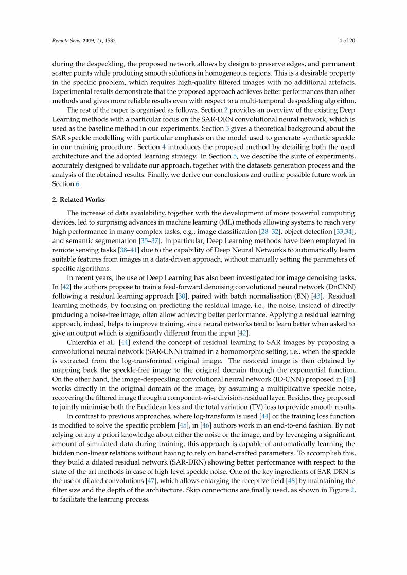
In contrast to previous approaches, where log-transform is used [44] or the training loss functionis modified to solve the specific problem [45], in [46] authors work in an end-to-end fashion. By notrelying on any a priori knowledge about either the noise or the image, and by leveraging a significantamount of simulated data during training, this approach is capable of automatically learning thehidden non-linear relations without having to rely on hand-crafted parameters. To accomplish this,they build a dilated residual network (SAR-DRN) showing better performance with respect to thestate-of-the-art methods in case of high-level speckle noise. One of the key ingredients of SAR-DRN isthe use of dilated convolutions [47], which allows enlarging the receptive field [48] by maintaining thefilter size and the depth of the architecture. Skip connections are finally used, as shown in Figure 2,to facilitate the learning process.

Remote Sens. 2019, 11, 1532 5 of 20

Figure 2. SAR-DRN architecture.

3. Speckle Model for Data Generation

Our approach follows the Supervised Learning (SL) paradigm, that is the task of learning amapping between pairs of inputs and the corresponding targets (ground truth). This is done in adata-driven fashion by feeding the algorithm with examples coming from a well-designed trainingset and minimising the error between the network predictions and the expected outputs. In theconsidered problem, the task is to learn a mapping between the speckled images and the speckle-freeones. The quality of the learned model is strongly related to the quality and variability of examplesused during training. A large number of speckled images, coupled with their speckle-free counterparts,are indeed needed to train DL models properly. Fortunately, thanks to the numerous EO missions(e.g., Sentinel-1, COSMO-SkyMed, RADARSAT, TERRASAR-X), petabytes of speckled SAR images arenowadays available. However, it is not physically possible to have their corresponding speckle-freeimages. Different approaches have been proposed to overcome this issue. Chierchia et al. [44]obtain speckle-free targets by averaging multi-temporal images and considering during trainingonly those regions that do not significantly change over time. Even if the obtained results arequalitatively promising, this approach strictly relies on the choice of patches, and it is limited bythe approximation made by considering the average image as the speckle-free reference. Otherworks [45,46] synthetically generate the speckle images by using prior knowledge about the statisticalmodel of the noise. Our approach builds on the same concept by using prior statistics about the speckleto generate synthetic images in the original SAR high-resolution space. In the following subsections,we briefly describe the speckle model we adopted and how it is applied for building the dataset weused during training.

3.1. Speckle Model

The most commonly adopted model for describing SAR speckle for distributed scatterers is themultiplicative noise model [49]

Y = NX (1)

where Y ∈ RW×H is the observed intensity image, X ∈ RW×H is the noise-free radar reflectivity imageand N ∈ RW×H is the speckle noise random variable. Assuming a L-looks SAR image, N followsa Gamma distribution with unit mean and variance 1/L with the following probability densityfunction [50]:

p(N) =LLNL−1e−LN

Γ(L), N ≥ 0, L ≥ 1 (2)

where Γ(·) denotes the Gamma function.The same multiplicative speckle noise model holds for an amplitude image (the square root of

the intensity)y = n · x (3)

Remote Sens. 2019, 11, 1532 6 of 20

where x is the speckle-free amplitude value. Now the speckle noise random variable n obeys to theNakagami distribution with the following probability density function

p(n) =2LLn2L−1e−Ln2

Γ(L), n ≥ 0, L ≥ 1 (4)

which results in the Rayleigh distribution in the case of single look (L = 1) amplitude image.

3.2. Speckled Image Simulation

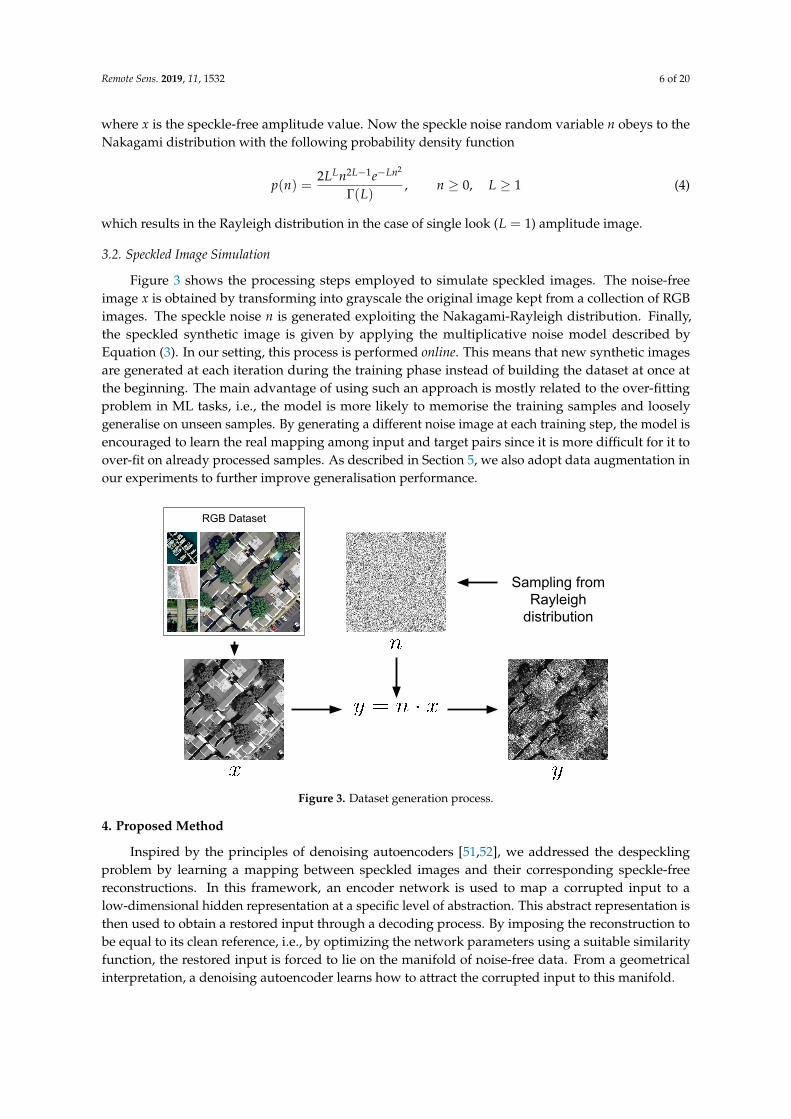
Figure 3 shows the processing steps employed to simulate speckled images. The noise-freeimage x is obtained by transforming into grayscale the original image kept from a collection of RGBimages. The speckle noise n is generated exploiting the Nakagami-Rayleigh distribution. Finally,the speckled synthetic image is given by applying the multiplicative noise model described byEquation (3). In our setting, this process is performed online. This means that new synthetic imagesare generated at each iteration during the training phase instead of building the dataset at once atthe beginning. The main advantage of using such an approach is mostly related to the over-fittingproblem in ML tasks, i.e., the model is more likely to memorise the training samples and looselygeneralise on unseen samples. By generating a different noise image at each training step, the model isencouraged to learn the real mapping among input and target pairs since it is more difficult for it toover-fit on already processed samples. As described in Section 5, we also adopt data augmentation inour experiments to further improve generalisation performance.

RGB Dataset

Sampling from Rayleigh

distribution

Figure 3. Dataset generation process.

4. Proposed Method

Inspired by the principles of denoising autoencoders [51,52], we addressed the despecklingproblem by learning a mapping between speckled images and their corresponding speckle-freereconstructions. In this framework, an encoder network is used to map a corrupted input to alow-dimensional hidden representation at a specific level of abstraction. This abstract representation isthen used to obtain a restored input through a decoding process. By imposing the reconstruction tobe equal to its clean reference, i.e., by optimizing the network parameters using a suitable similarityfunction, the restored input is forced to lie on the manifold of noise-free data. From a geometricalinterpretation, a denoising autoencoder learns how to attract the corrupted input to this manifold.

Remote Sens. 2019, 11, 1532 7 of 20

The same concepts can be applied in the SAR image despeckling task, by employing asuitable architecture to extract latent representations from speckled images and by obtaining theircorresponding reconstructions. In particular, we developed a modified version of U-Net, which is anencoder–decoder convolutional neural network initially designed for biomedical image segmentationtasks [27]. The U-Net’s encoder network allows compressing the information by extracting relevantfeatures from the input image at different scales, thus providing representations at different levelsof abstraction. The decoder network performs the corresponding reconstruction by mapping backthe latent representation to the input spatial resolution. This process is done by stacking severalupsampling layers, each of them restoring the information at different resolution. During the encodingprocess, part of the information could be lost, especially when using a deep network. Then, the decodercould be not able to recover details of the given image starting from its abstract representation.To this purpose, U-Net provides a set of skip connections which allow preserving relevant informationduring the decoding stage, thus enhancing the accuracy of the restored image. We provide moreinsights into the role of skip connections in Section 5.5.1.

4.1. Architecture

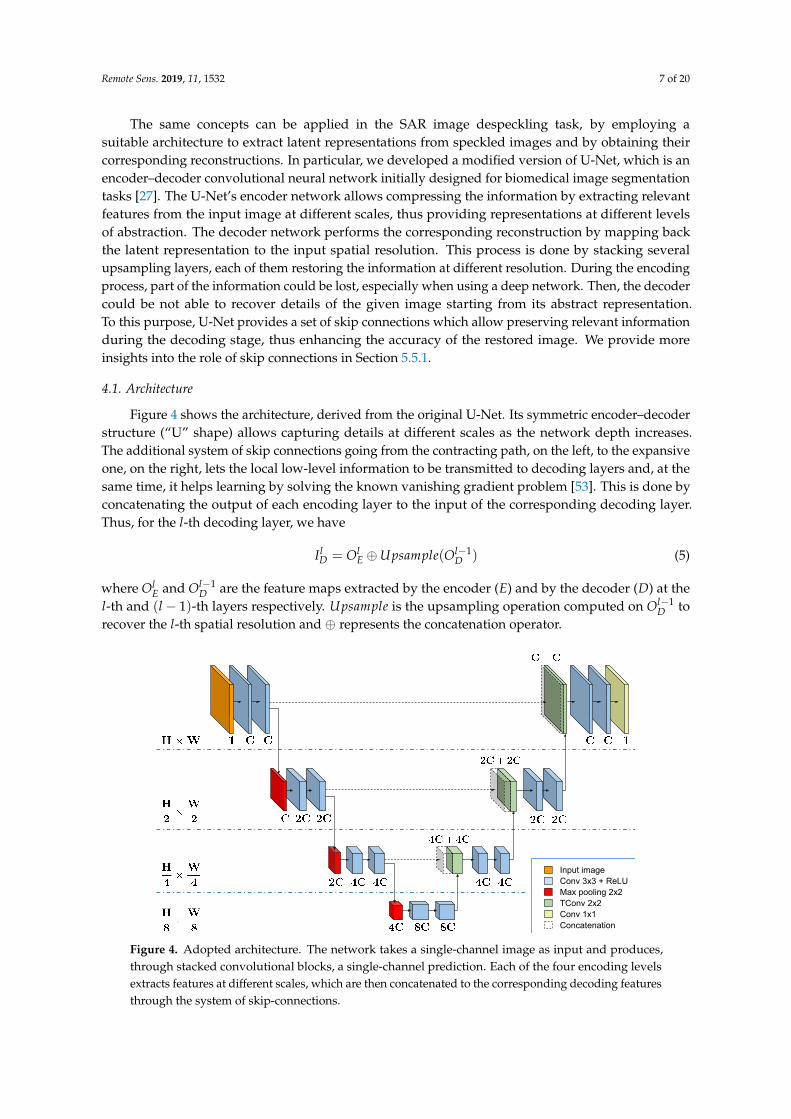
Figure 4 shows the architecture, derived from the original U-Net. Its symmetric encoder–decoderstructure (“U” shape) allows capturing details at different scales as the network depth increases.The additional system of skip connections going from the contracting path, on the left, to the expansiveone, on the right, lets the local low-level information to be transmitted to decoding layers and, at thesame time, it helps learning by solving the known vanishing gradient problem [53]. This is done byconcatenating the output of each encoding layer to the input of the corresponding decoding layer.Thus, for the l-th decoding layer, we have

IlD = Ol

E ⊕Upsample(Ol−1D ) (5)

where OlE and Ol−1

D are the feature maps extracted by the encoder (E) and by the decoder (D) at thel-th and (l − 1)-th layers respectively. Upsample is the upsampling operation computed on Ol−1

D torecover the l-th spatial resolution and ⊕ represents the concatenation operator.

Conv 3x3 + ReLUMax pooling 2x2TConv 2x2Conv 1x1

Input image

Concatenation

Figure 4. Adopted architecture. The network takes a single-channel image as input and produces,through stacked convolutional blocks, a single-channel prediction. Each of the four encoding levelsextracts features at different scales, which are then concatenated to the corresponding decoding featuresthrough the system of skip-connections.

Remote Sens. 2019, 11, 1532 8 of 20

We modified the original U-Net architecture by using a four-layer structure for the contractivepart, which is one level less than the depth of the original network. In addition, we changed the firstconvolutional layer to deal with one-channel input images. Each layer of the encoding path, except forthe input layer, takes as input the output feature maps of the previous layer and, after compressingthem through a downsampling operation, it produces as output a tensor of feature maps with doublethe channels. Thus, at each level

OlE = EncBlock(Ol−1

E ) (6)

where Ol−1E of dimension Hl−1 ×W l−1 × Cl−1 is the output of the previous encoding layer and Ol

E are

the feature maps extracted at the current level with dimension H2

l−1 × W2

l−1 × 2 · Cl−1. EncBlock isthe encoding block composed by a max-pooling layer followed by two stacked convolutional layers.Since the number of features extracted by the first encoding layer is set to 64, we obtain 512 features asoutput of the contractive path. In Section 5.5.1 we performed an ablation study on different networkconfigurations, i.e., different depth levels and number of feature maps for each layer.

The decoder network mirrors the encoder. The output of the previous decoding layer Ol−1D is first

upsampled by applying a 2× 2 Transposed Convolution (TConv) layer [54] which produces a set offeature maps of the same dimension of the output of the l-th encoding layer. Then, after applying theconcatenation layer (Equation (5)), the final output is obtained by applying two stacked convolutionallayers. Each layer uses 3× 3 filters and stride equal to one except for the final convolutional layerwhich use a 1× 1 filter to produce a prediction in the original input space. The non-linear activationemployed after each convolution, except for the last one in which a linear activation is used instead, isthe rectified linear unit (ReLU) which is defined as

ReLU(x) = max(0, x). (7)

4.2. Learning

The procedure adopted to learn the parameters of the proposed network belongs to the residuallearning paradigm, which proved to be effective in previous related works. Thus, the architectureis trained to extract the noise from the noisy input image instead of directly learning the mappingbetween input and corresponding clean image. Contrary to homomorphic approaches, in whichthe multiplicative speckle model is first converted into an additive one through the logarithmictransformation of the input, here we adopt the same residual strategy as SAR-DRN. The residual noiseis expressed as the difference between noisy and clean images. Therefore

n = y− x, (8)

where n is the residual image, x is the clean target, and y is the speckled input. Accordingly, the networkis trained to find the function

φ(y, θ) = n̂ (9)

where θ are the model parameters, that are trained to approximate as well as possible the real mappingbetween input y and the target residual noise n. This is done in a supervised fashion by minimising theerror between the predicted residual image and the target one. In particular, we used the mean-squarederror (MSE) defined as

loss(n̂, n) =1

2N

N

∑i=1‖φ(yi, θ)− ni‖2

2 . (10)

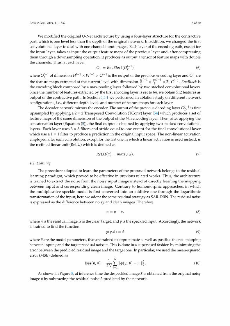
As shown in Figure 5, at inference time the despeckled image x̂ is obtained from the original noisyimage y by subtracting the residual noise n̂ predicted by the network.

Remote Sens. 2019, 11, 1532 9 of 20

Figure 5. Despeckling procedure.

5. Experimental Results

In order to evaluate the performance of our model, we designed a suitable set of experimentswhich covers synthetic and real image despeckling domains. In particular, we built two types ofdatasets, one for each domain, to asses the quality of our predictions, both when dealing with syntheticimages and real SAR ones. The synthetic dataset allows to numerically compare the quality of ourpredictions with state-of-the-art approaches, while the latter is intended to demonstrate how theproposed architecture can be successfully employed in a real despeckling scenario. In the following,we give an overview of the datasets we generated to run the experiments, and we present our mainresults together with the comparison with state-of-the-art methods.

5.1. Synthetic Dataset

The synthetic dataset has been built using aerial images from the UC Merced dataset [55] createdfor land use classification. The original dataset is composed of RGB images taken from the USGSNational Map Urban Area Imagery collection and subdivided into 21 classes depending on the typeof the land. From this dataset, we selected 1409 images from which we extracted 238,121 patches of64× 64 pixels as the training set. Furthermore, we selected 294 images of 256× 256 pixels from threeclasses (Airplane, Buildings, and River) that are not used for training to perform the validation. Besides,we built a test set for the very final validation using four images from the PatternNet dataset [56],which are taken from unseen classes (Transformer Station, Basketball Court, Tree Farm, and Bridge).The test set is used to compare our performance with state-of-the-art methods.

As anticipated in Section 3.2, we use the training set to generate single look synthetic speckledimages using the online procedure depicted in Figure 3. Furthermore, at each training step the samplesare augmented before to be fed to the network by randomly combining horizontal and vertical flipping,90◦ and 270◦ rotation, and changes in image contrast. As shown in the ablation study, the performanceincreases as the data augmentation becomes more severe.

5.2. Real SAR Dataset

We built an additional dataset to fine-tune the learned model on the specific real SAR domain,which is characterised by high-resolution images. The challenge to be faced was to create thecorresponding pairs of speckled and target images for training that had to be as similar as possibleto real images. Since it is not physically possible to obtain a despeckled realisation of SAR images,we adopted an alternative strategy to obtain a speckle free reference to train the model. Specifically,we considered the point-wise temporal average over a stack of SAR images as the target image.

Remote Sens. 2019, 11, 1532 10 of 20

The noise is then generated synthetically as in the case of aerial data. Even if the data is simulated,the obtained dataset provides samples that are close to the real ones, allowing the model to handlehigh-resolution images better.

We considered two large temporal stacks provided by the Sentinel-1 mission that have beenaveraged to generate two despeckled images with a resolution of 20 × 5 m (VV polarisation).The dimensions of the two images are 31,576 × 7251 and 40,439 × 15,340 pixels, respectively.We extracted 167,713 patches of 64× 64 pixels as training set and 16,856 patches as the validation set.The latter has been incremented with additional unseen images computed with the simulation processfor a total of 26,901 validation patches. Finally, we built a suitable test set to evaluate the proposedapproach on real single look SAR images. To this purpose, we collected other Sentinel-1 images and alsoimages coming from different constellations, in the specific COSMO-SkyMed (CSK) and RADARSAT(HH polarisation), to evaluate the generalisation capability of the network on different resolutions.

5.3. Training

Our best result is achieved by using the four-level U-Net configuration with 64 features extractedat the first encoding layer. We employed a minibatch learning procedure by creating batchesof 128 samples. The update of the network parameters was performed using the Adam [57]gradient-based optimisation algorithm with β1 = 0.9, β2 = 0.999, and ε = 10−8, where β1 andβ2 are the exponential decay rates for the first and second moment estimates respectively while ε

prevents any division by zero in the implementation. Thus, at each iteration t, the network parametersare updated using the following formulation

θt+1 = θt − ηm̂t+1

(√

v̂t+1 + ε)(11)

where η is the learning rate and m̂t+1 and v̂t+1 are the bias-corrected first and second raw momentestimates defined as

m̂t+1 =β1mt + (1− β1)gt+1

(1− βt+11 )

(12)

v̂t+1 =β2vt + (1− β2)g2

t+1

(1− βt+12 )

(13)

where gt+1 are the gradients of the objective function at time t with respect to the network parameters θ.In particular, denoting the MSE function introduced in Equation (10) as the data fitting loss LD,the gradients are computed as

gt+1 = ∇θ LD(θt) =∂LD(θt)

∂θ=

1N

N

∑i=1

(φ(yi, θt)− ni)∂φ(yi, θt)

∂θ. (14)

The network has been trained on the synthetic dataset for 50 epochs, for a total of 93,050 training steps,using η = 0.001 as starting learning rate. We further adopted a learning rate decay schedule bydecreasing it of 0.5 at intervals of 10 epochs.

For what concern the experiments on real SAR images, we used the parameters learned on theaerial dataset as initialisation, instead of training a new model from scratch. In this way, we tookadvantage of the already acquired capability of the model to extract relevant features for noise removal,and we fine-tuned the network parameters to deal with images in the real domain. This process is alsoknown as domain adaptation, and it requires only a few additional training steps. Also, in this case,we employed a minibatch learning using batches of 128 samples each. The network has been fine-tunedfor 15 epochs using a learning rate of 5 · 10−6 and the Adam optimiser with the same hyper-parametersof the synthetic experiments.

Remote Sens. 2019, 11, 1532 11 of 20

In the real domain, the speckle noise has some properties that are not fully captured by thesynthetically generated images. For this reason, despite the good capability of the network in filteringthe speckle, the generated images still contain some blurry artefacts. Thus, we introduce a TotalVariation (TV) regularisation loss during the training with the goal of removing the artefacts andproducing smoother results while preserving the structure and the details of the images. The TV lossis defined as

LTV = ∑i,j

e−|∇hxij ||∇h x̂ij|+ e−|∇vxij ||∇v x̂ij| (15)

where ∇h x̂ and ∇v x̂ are the gradients of the reconstructed image on the horizontal and verticaldirections, respectively, and are defined as

∇h x̂ij = x̂i,j+1 − x̂i,j (16)

∇v x̂ij = x̂i+1,j − x̂i,j (17)

while ∇hx and ∇vx are the gradients computed on the speckle-free reference image on the samedirections. The role of the former is to minimise the difference among neighbouring pixels whilethe latter allows avoiding over-smoothed results in correspondence of the edges. The total costfunction becomes

L = LD + λTV LTV (18)

where LD is the data fitting term defined in Equation (10) while λTV is the hyper-parameter governingthe importance of the regularisation. We initially performed a random search to find the range ofvalues of λTV for which TV gives a relevant contribution, finding 1 · 10−4 ≤ λTV ≤ 5 · 10−4. Finally,we found λTV = 2 · 10−4 to give the best regularisation incidence in our experiments. Also in this casewe compute the gradients gt+1 of the objective function at time t as

gt+1 = ∇θ L(θt) = ∇θ LD(θt) + λTV∇θ LTV(θt). (19)

where ∇θ LD(θt) are computed as in Equation (14), while the gradients of the total variation aregiven by

∇θ LTV(θt) =∂LTV(θt)

∂θ= ∑

i,je−|∇hxij | ∇h x̂ij

|∇h x̂ij|∂∇h x̂ij

∂θ+ e−|∇vxij | ∇v x̂ij

|∇v x̂ij|∂∇v x̂ij

∂θ(20)

5.4. Metrics for Evaluation

In the aerial dataset, the target corresponding to each noisy image is available since the latterare generated synthetically. Thus, it is possible to evaluate the quality of the provided approach bycomputing two kinds of metrics that are typically used in image denoising tasks. They are the peaksignal-to-noise ratio (PSNR) and the structural similarity (SSIM) index. The PSNR expresses the ratiobetween the maximum signal power and the power of the noise affecting its quality. It measures howclosely the reconstructed image represents the original one and is given by

PSNR = 20 log10

(MAXI√

MSE

)(21)

where MAXI is the maximum signal power, i.e., 255 for grayscale images and the MSE is computedbetween the noise-free target image and its reconstruction. The SSIM measures instead of the similaritybetween two images from the point of view of their structural information, i.e., the structure ofobjects in the scene, regardless of the changes in contrast and luminance. Given two images x and y,it is defined as

Remote Sens. 2019, 11, 1532 12 of 20

SSIM(x, y) =

(2µxµy + c1

) (2σxy + c2

)(µ2

x + µ2y + c1

) (σ2

x + σ2y + c2

) (22)

where µi is the mean of i, σi is the variance of i, and ci is a constant introduced to avoid instabilities.Since a speckle-free reference is not available in the real domain, it is not possible to compute

the metrics introduced above. A different approach is thus required. One option remains the visualinspection of the reconstructed images, for which we provide several results on different scenarios.Another common approach, that we adopted in this work, is to evaluate the degree of smoothing in ahomogeneous region by computing the equivalent number of looks (ENL) defined as

ENL(I) =µ2

Iσ2

I(23)

where µI and σI are the mean and standard deviation of the considered image portion I respectively.The main difficulty in the computation of this metric is the ability to find a considerable homogeneousregion inside the image under evaluation.

5.5. Results on Synthetic Images

We compare the performance of our approach with the one of two methods: SAR-BM3D,belonging to the class of algorithms of non-learned filters, and SAR-DRN, which is, to the bestof our knowledge, the state-of-the-art method among DL approaches. For the former we used thepublicly available MATLAB code http://www.grip.unina.it/research/80-sar-despeckling/80-sar-bm3d.html,setting the parameters as suggested in the original paper. For what concern SAR-DRN, instead, nopublic code is available. We thus implemented and trained SAR-DRN from scratch on our dataset,following the specifics given by the authors in the reference paper.

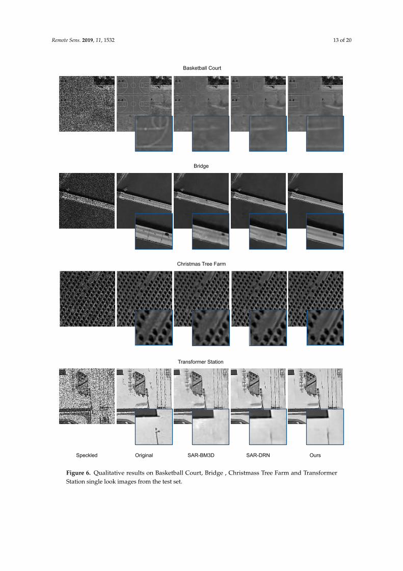
Figure 6 shows the qualitative results of our approach on a selection of the test set, together withthe ones of selected methods. Notice that, even if SAR-BM3D is quite effective in removing the specklenoise, the filtered images loosely preserve the object details and smoothness in homogeneous regions.SAR-DRN shows better performance w.r.t. SAR-BM3D, filtering out the speckle with higher accuracy.However, the produced images are still contaminated by some blurry artefacts. The proposed network,thanks to the combined action of its encoder–decoder structure and the system of skip-connections,improves the quality of the despeckled images by providing sharper results in correspondence ofedges and preserving homogeneity among spatially coherent pixels (e.g., Bridge).

The qualitative improvements are reflected by the numerical results. As shown in Table 1,our approach shows a gain in the PSNR metric of about 1.21 dB, 0.80 dB, 1.68 dB, and 1.87 dB w.r.t.SAR-BM3D algorithm for Bridge, Basketball Court, Christmas Tree Farm, and Transformer Stationrespectively and outperforms SAR-DRN of about 0.63 dB, 0.20 dB, 0.62 dB, and 0.28 dB in the sameimages. These improvements testify a better image restoration capability compared with other methods.The proposed approach outperforms the baseline methods also in terms of SSIM index, as highlightedin Table 2, providing more accurate preservation of the image structural information.

Table 1. PSNR computed on test set.

Bridge Basketball Court Christmas Tree Farm Transformer Station

mean std mean std mean std mean std

Noisy 18.3489 0.0354 14.6548 0.0211 17.6521 0.0289 10.7685 0.0235

SAR-BM3D 29.6914 0.1222 28.7579 0.0516 28.2377 0.0733 20.4701 0.0627

SAR-DRN 30.2771 0.1271 29.3548 0.0995 29.3019 0.0524 22.0661 0.0588

Ours 30.9079 0.1122 29.5644 0.0906 29.9250 0.0915 22.3491 0.0316

Remote Sens. 2019, 11, 1532 13 of 20

OriginalSpeckled SAR-BM3D SAR-DRN Ours

Basketball Court

Bridge

Christmas Tree Farm

Transformer Station

Figure 6. Qualitative results on Basketball Court, Bridge , Christmass Tree Farm and TransformerStation single look images from the test set.

Remote Sens. 2019, 11, 1532 14 of 20

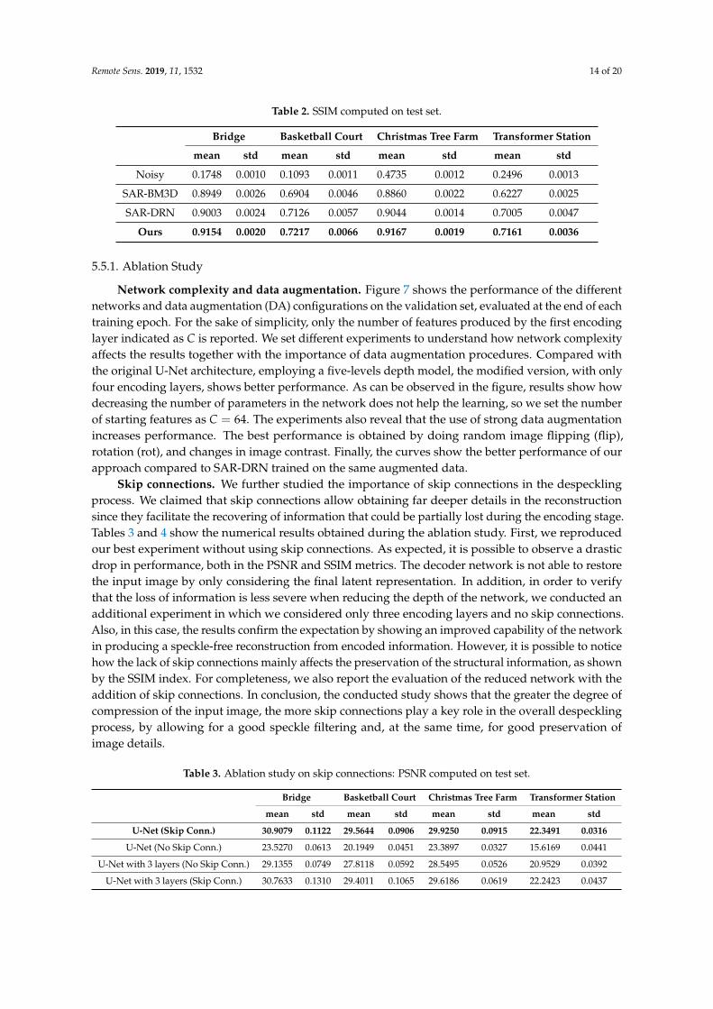
Table 2. SSIM computed on test set.

Bridge Basketball Court Christmas Tree Farm Transformer Station

mean std mean std mean std mean std

Noisy 0.1748 0.0010 0.1093 0.0011 0.4735 0.0012 0.2496 0.0013

SAR-BM3D 0.8949 0.0026 0.6904 0.0046 0.8860 0.0022 0.6227 0.0025

SAR-DRN 0.9003 0.0024 0.7126 0.0057 0.9044 0.0014 0.7005 0.0047

Ours 0.9154 0.0020 0.7217 0.0066 0.9167 0.0019 0.7161 0.0036

5.5.1. Ablation Study

Network complexity and data augmentation. Figure 7 shows the performance of the differentnetworks and data augmentation (DA) configurations on the validation set, evaluated at the end of eachtraining epoch. For the sake of simplicity, only the number of features produced by the first encodinglayer indicated as C is reported. We set different experiments to understand how network complexityaffects the results together with the importance of data augmentation procedures. Compared withthe original U-Net architecture, employing a five-levels depth model, the modified version, with onlyfour encoding layers, shows better performance. As can be observed in the figure, results show howdecreasing the number of parameters in the network does not help the learning, so we set the numberof starting features as C = 64. The experiments also reveal that the use of strong data augmentationincreases performance. The best performance is obtained by doing random image flipping (flip),rotation (rot), and changes in image contrast. Finally, the curves show the better performance of ourapproach compared to SAR-DRN trained on the same augmented data.

Skip connections. We further studied the importance of skip connections in the despecklingprocess. We claimed that skip connections allow obtaining far deeper details in the reconstructionsince they facilitate the recovering of information that could be partially lost during the encoding stage.Tables 3 and 4 show the numerical results obtained during the ablation study. First, we reproducedour best experiment without using skip connections. As expected, it is possible to observe a drasticdrop in performance, both in the PSNR and SSIM metrics. The decoder network is not able to restorethe input image by only considering the final latent representation. In addition, in order to verifythat the loss of information is less severe when reducing the depth of the network, we conducted anadditional experiment in which we considered only three encoding layers and no skip connections.Also, in this case, the results confirm the expectation by showing an improved capability of the networkin producing a speckle-free reconstruction from encoded information. However, it is possible to noticehow the lack of skip connections mainly affects the preservation of the structural information, as shownby the SSIM index. For completeness, we also report the evaluation of the reduced network with theaddition of skip connections. In conclusion, the conducted study shows that the greater the degree ofcompression of the input image, the more skip connections play a key role in the overall despecklingprocess, by allowing for a good speckle filtering and, at the same time, for good preservation ofimage details.

Table 3. Ablation study on skip connections: PSNR computed on test set.

Bridge Basketball Court Christmas Tree Farm Transformer Station

mean std mean std mean std mean std

U-Net (Skip Conn.) 30.9079 0.1122 29.5644 0.0906 29.9250 0.0915 22.3491 0.0316

U-Net (No Skip Conn.) 23.5270 0.0613 20.1949 0.0451 23.3897 0.0327 15.6169 0.0441

U-Net with 3 layers (No Skip Conn.) 29.1355 0.0749 27.8118 0.0592 28.5495 0.0526 20.9529 0.0392

U-Net with 3 layers (Skip Conn.) 30.7633 0.1310 29.4011 0.1065 29.6186 0.0619 22.2423 0.0437

Remote Sens. 2019, 11, 1532 15 of 20

PN

SR

(dB

)

Epochs

U-Net, 4 levels, C = 64, DA = flip + rot + contrast

U-Net, 4 levels, C = 64, DA = flip + rot

U-Net, 4 levels, C = 64, DA = flip

U-Net, 4 levels, C = 32, DA = flip

U-Net, 4 levels, C = 16, DA = flip

U-Net, 5 levels, C = 64, DA = flip

SAR-DRN, DA = flip + rot + contrast

26.0

25.9

25.8

25.7

25.6

25.5

25.4

25.3

25.2

25.1

25.0

0.000 10.00 20.00 30.00 40.00 50.00

Figure 7. Ablation: network configurations and data augmentation.

Table 4. Ablation study on skip connections: SSIM computed on test set.

Bridge Basketball Court Christmas Tree Farm Transformer Station

mean std mean std mean std mean std

U-Net (Skip Conn.) 0.9154 0.0020 0.7217 0.0066 0.9167 0.0019 0.7161 0.0036

U-Net (No Skip Conn.) 0.3195 0.0020 0.1992 0.0037 0.6916 0.0030 0.3258 0.0019

U-Net with 3 layers (No Skip Conn.) 0.7457 0.0158 0.5143 0.0175 0.8663 0.0023 0.5145 0.0038

U-Net with 3 layers (Skip Conn.) 0.8917 0.0055 0.6610 0.0152 0.8964 0.0027 0.7076 0.0052

5.5.2. Results on Real SAR Images

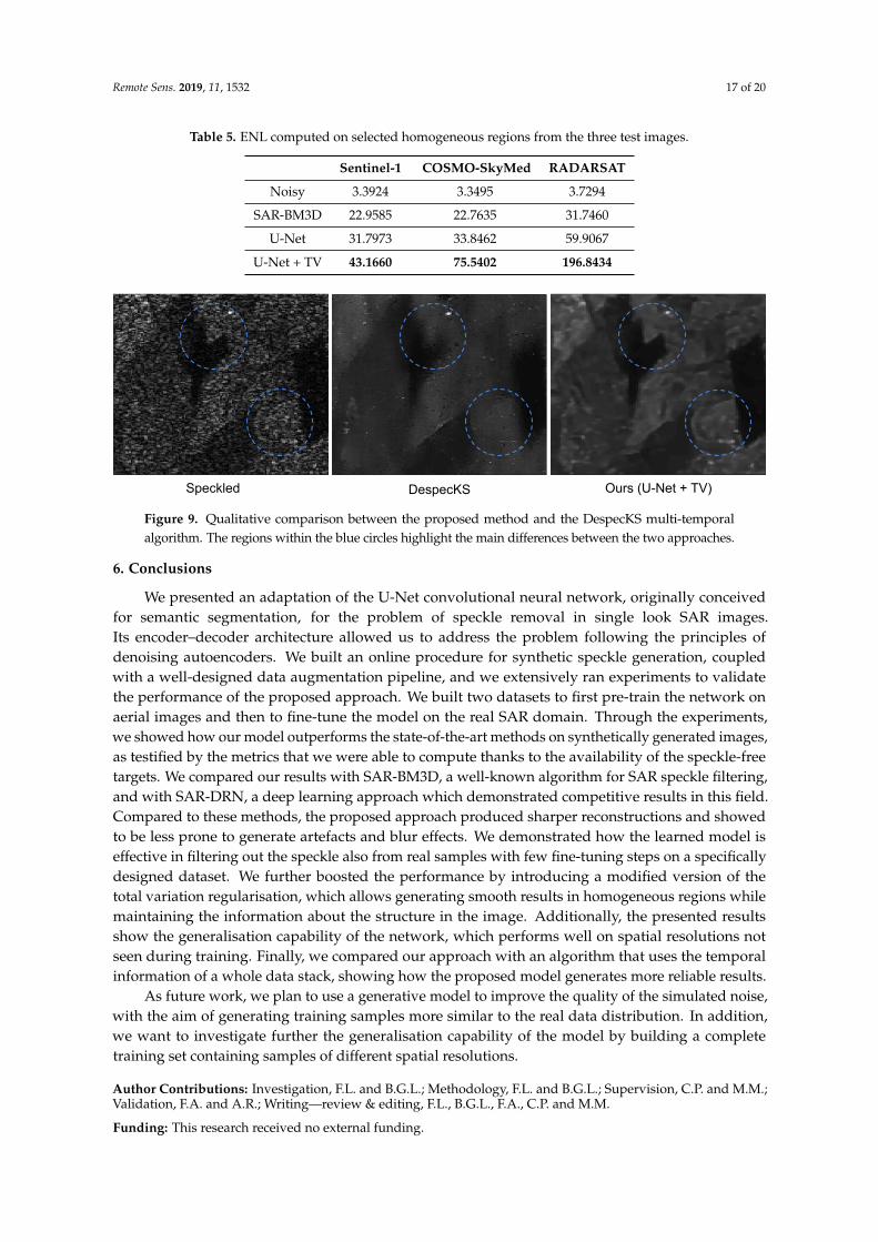
Figure 8 shows the qualitative results on different single look SAR images. It is possible to observehow the SAR-BM3D algorithm is quite efficient in removing the speckle, but the reconstructed imagesstill contain some residual noise as testified by the produced artefacts. The base version of the proposedU-Net architecture, i.e., without TV, shows visually better results by generating sharper images. It isinteresting to notice how the proposed approach performs well also on images having a spatialresolution different from the one encountered during the training phase. The performance achievedon the Sentinel-1 image, having a resolution of 20× 5 m, is also achieved on the COSMO-SkyMedand RADARSAT images, having a resolution of 3× 3 and 15× 15 m, respectively. The best resultswere given by the model learned with the TV regularization whose reconstructions are smoother onhomogeneous areas, further removing some of the residual artefacts, while preserving the structure ofthe images. The quantitative results proposed in Table 5 reflects the above considerations showing howthe proposed approach has higher performance in speckle suppression in the considered homogeneousregions. Figure 9 shows a qualitative comparison between our single observation approach and theDespecKS algorithm based on multi-temporal data. As highlighted by the blue circles, the proposedmodel has a higher capability of preserving the information contained in the image while the referencealgorithm tends to lose the details due to the averaging over the temporal dimension. Our approachprovides faster and more accurate results by looking only to a single image instead of processing theentire data stack.

Remote Sens. 2019, 11, 1532 16 of 20

Speckled

SAR-BM3D

Ours (U-Net)

Ours (U-Net + TV)

Figure 8. Qualitative results on Sentinel-1 (1-st column), COSMO-SkyMed (2-nd column), and RADARSAT(3-th column) single look images from the test set. The red boxes point out the homogeneous regionsselected for the computation of the ENL metric. As can be observed, the reconstructions provided by theproposed method are sharper and less affected by residual artefacts.

Remote Sens. 2019, 11, 1532 17 of 20

Table 5. ENL computed on selected homogeneous regions from the three test images.

Sentinel-1 COSMO-SkyMed RADARSAT

Noisy 3.3924 3.3495 3.7294

SAR-BM3D 22.9585 22.7635 31.7460

U-Net 31.7973 33.8462 59.9067

U-Net + TV 43.1660 75.5402 196.8434

Speckled Ours (U-Net + TV)DespecKS

Figure 9. Qualitative comparison between the proposed method and the DespecKS multi-temporalalgorithm. The regions within the blue circles highlight the main differences between the two approaches.

6. Conclusions

We presented an adaptation of the U-Net convolutional neural network, originally conceivedfor semantic segmentation, for the problem of speckle removal in single look SAR images.Its encoder–decoder architecture allowed us to address the problem following the principles ofdenoising autoencoders. We built an online procedure for synthetic speckle generation, coupledwith a well-designed data augmentation pipeline, and we extensively ran experiments to validatethe performance of the proposed approach. We built two datasets to first pre-train the network onaerial images and then to fine-tune the model on the real SAR domain. Through the experiments,we showed how our model outperforms the state-of-the-art methods on synthetically generated images,as testified by the metrics that we were able to compute thanks to the availability of the speckle-freetargets. We compared our results with SAR-BM3D, a well-known algorithm for SAR speckle filtering,and with SAR-DRN, a deep learning approach which demonstrated competitive results in this field.Compared to these methods, the proposed approach produced sharper reconstructions and showedto be less prone to generate artefacts and blur effects. We demonstrated how the learned model iseffective in filtering out the speckle also from real samples with few fine-tuning steps on a specificallydesigned dataset. We further boosted the performance by introducing a modified version of thetotal variation regularisation, which allows generating smooth results in homogeneous regions whilemaintaining the information about the structure in the image. Additionally, the presented resultsshow the generalisation capability of the network, which performs well on spatial resolutions notseen during training. Finally, we compared our approach with an algorithm that uses the temporalinformation of a whole data stack, showing how the proposed model generates more reliable results.

As future work, we plan to use a generative model to improve the quality of the simulated noise,with the aim of generating training samples more similar to the real data distribution. In addition,we want to investigate further the generalisation capability of the model by building a completetraining set containing samples of different spatial resolutions.

Author Contributions: Investigation, F.L. and B.G.L.; Methodology, F.L. and B.G.L.; Supervision, C.P. and M.M.;Validation, F.A. and A.R.; Writing—review & editing, F.L., B.G.L., F.A., C.P. and M.M.

Funding: This research received no external funding.

Remote Sens. 2019, 11, 1532 18 of 20

Acknowledgments: We would like to thank TRE ALTAMIRA s.r.l. for providing the data and for the assistanceduring the evaluation process. An additional thanks goes to Andrea Romanoni, Marco Cannici and Marco Cicconefor their useful suggestions during the review of the article.

Conflicts of Interest: The authors declare no conflict of interest.

References

1. Bamler, R.; Hartl, P. Synthetic aperture radar interferometry. Inverse Probl. 1998, 14, R1–R54. [CrossRef]2. Lee, J. Digital Image Enhancement and Noise Filtering by Use of Local Statistics. IEEE Trans. Pattern Anal.

Mach. Intell. 1980, PAMI-2, 165–168. [CrossRef]3. Kuan, D.T.; Sawchuk, A.A.; Strand, T.C.; Chavel, P. Adaptive Noise Smoothing Filter for Images with

Signal-Dependent Noise. IEEE Trans. Pattern Anal. Mach. Intell. 1985, PAMI-7, 165–177. [CrossRef]4. Frost, V.S.; Stiles, J.A.; Shanmugan, K.S.; Holtzman, J.C. A Model for Radar Images and Its Application

to Adaptive Digital Filtering of Multiplicative Noise. IEEE Trans. Pattern Anal. Mach. Intell. 1982,PAMI-4, 157–166. [CrossRef]

5. Shi, Z.; Fung, K.B. A comparison of digital speckle filters. In Proceedings of IGARSS ’94—1994 IEEEInternational Geoscience and Remote Sensing Symposium, Pasadena, CA, USA, 8–12 August 1994; Volumr 4,pp. 2129–2133. [CrossRef]

6. Lopes, A.; Touzi, R.; Nezry, E. Adaptive speckle filters and scene heterogeneity. IEEE Trans. Geosci.Remote Sens. 1990, 28, 992–1000. [CrossRef]

7. Xie, H.; Pierce, L.E.; Ulaby, F.T. SAR speckle reduction using wavelet denoising and Markov random fieldmodeling. IEEE Trans. Geosci. Remote Sens. 2002, 40, 2196–2212. [CrossRef]

8. Espinoza Molina, D.; Gleich, D.; Datcu, M. Evaluation of Bayesian Despeckling and Texture ExtractionMethods Based on Gauss–Markov and Auto-Binomial Gibbs Random Fields: Application to TerraSAR-XData. IEEE Trans. Geosci. Remote Sens. 2012, 50, 2001–2025. [CrossRef]

9. Mahdianpari, M.; Salehi, B.; Mohammadimanesh, F. The Effect of PolSAR Image De-speckling onWetland Classification: Introducing a New Adaptive Method. Can. J. Remote Sens. 2017, 43, 485–503,doi:10.1080/07038992.2017.1381549. [CrossRef]

10. Argenti, F.; Alparone, L. Speckle removal from SAR images in the undecimated wavelet domain. IEEE Trans.Geosci. Remote Sens. 2002, 40, 2363–2374. [CrossRef]

11. Solbo, S.; Eltoft, T. Homomorphic wavelet-based statistical despeckling of SAR images. IEEE Trans. Geosci.Remote Sens. 2004, 42, 711–721. [CrossRef]

12. Lopes, A.; Nezry, E.; Touzi, R.; Laur, H. Maximum A Posteriori Speckle Filtering And First Order TextureModels In Sar Images. In Proceedings of the 10th Annual International Symposium on Geoscience andRemote Sensing, College Park, MD, USA, 20–24 May 1990; pp. 2409–2412. [CrossRef]

13. Buades, A.; Coll, B.; Morel, J. A non-local algorithm for image denoising. In Proceedings of the 2005 IEEEComputer Society Conference on Computer Vision and Pattern Recognition (CVPR’05), San Diego, CA, USA,20–25 June 2005; Volume 2, pp. 60–65. [CrossRef]

14. Deledalle, C.; Denis, L.; Tupin, F. Iterative Weighted Maximum Likelihood Denoising With ProbabilisticPatch-Based Weights. IEEE Trans. Image Process. 2009, 18, 2661–2672. [CrossRef] [PubMed]

15. Dabov, K.; Foi, A.; Katkovnik, V.; Egiazarian, K. Image Denoising by Sparse 3-D Transform-DomainCollaborative Filtering. IEEE Trans. Image Process. 2007, 16, 2080–2095. [CrossRef] [PubMed]

16. Parrilli, S.; Poderico, M.; Angelino, C.V.; Verdoliva, L. A Nonlocal SAR Image Denoising Algorithm Basedon LLMMSE Wavelet Shrinkage. IEEE Trans. Geosci. Remote Sens. 2012, 50, 606–616. [CrossRef]

17. Rudin, L.I.; Osher, S.; Fatemi, E. Nonlinear total variation based noise removal algorithms. Phys. DNonlinear Phenom. 1992, 60, 259–268. [CrossRef]

18. Aubert, G.; Aujol, J.F. A Variational Approach to Removing Multiplicative Noise. SIAM J. Appl. Math. 2008,68, 925–946. [CrossRef]

19. Steidl, G.; Teuber, T. Removing Multiplicative Noise by Douglas-Rachford Splitting Methods. J. Math.Imaging Vis. 2010, 36, 168–184. [CrossRef]

20. Bioucas-Dias, J.M.; Figueiredo, M.A.T. Multiplicative Noise Removal Using Variable Splitting andConstrained Optimization. IEEE Trans. Image Process. 2010, 19, 1720–1730. [CrossRef] [PubMed]

Remote Sens. 2019, 11, 1532 19 of 20

21. Shi, J.; Osher, S. A Nonlinear Inverse Scale Space Method for a Convex Multiplicative Noise Model. SIAM J.Img. Sci. 2008, 1, 294–321. [CrossRef]

22. Zhao, Y.; Liu, J.G.; Zhang, B.; Hong, W.; Wu, Y. Adaptive Total Variation Regularization Based SAR ImageDespeckling and Despeckling Evaluation Index. IEEE Trans. Geosci. Remote Sens. 2015, 53, 2765–2774.[CrossRef]

23. Palsson, F.; Sveinsson, J.R.; Ulfarsson, M.O.; Benediktsson, J.A. SAR image denoising using total variationbased regularization with sure-based optimization of the regularization parameter. In Proceedings of the2012 IEEE International Geoscience and Remote Sensing Symposium, Munich, Germany, 22–27 July 2012;pp. 2160–2163. [CrossRef]

24. Ferretti, A.; Fumagalli, A.; Novali, F.; Prati, C.; Rocca, F.; Rucci, A. A New Algorithm for ProcessingInterferometric Data-Stacks: SqueeSAR. IEEE Trans. Geosci. Remote Sens. 2011, 49, 3460–3470. [CrossRef]

25. Chierchia, G.; Gheche, M.E.; Scarpa, G.; Verdoliva, L. Multitemporal SAR Image Despeckling Based onBlock-Matching and Collaborative Filtering. IEEE Trans. Geosci. Remote Sens. 2017, 55, 5467–5480. [CrossRef]

26. Zhao, W.; Deledalle, C.A.; Denis, L.; Maître, H.; Nicolas, J.M.; Tupin, F. Ratio-based multi-temporal SARimages denoising. IEEE Trans. Geosci. Remote. Sens. 2018. [CrossRef]

27. Ronneberger, O.; Fischer, P.; Brox, T. U-net: Convolutional networks for biomedical image segmentation.In Proceedings of the International Conference on Medical Image Computing and Computer-AssistedIntervention, Munich, Germany, 5–9 October 2015; pp. 234–241.

28. Simonyan, K.; Zisserman, A. Very Deep Convolutional Networks for Large-Scale Image Recognition. arXiv2014, arXiv:1409.1556.

29. Szegedy, C.; Liu, W.; Jia, Y.; Sermanet, P.; Reed, S.; Anguelov, D.; Erhan, D.; Vanhoucke, V.; Rabinovich, A.Going deeper with convolutions. In Proceedings of the 2015 IEEE Conference on Computer Vision andPattern Recognition (CVPR), Boston, MA, USA, 7–12 June 2015; pp. 1–9. [CrossRef]

30. He, K.; Zhang, X.; Ren, S.; Sun, J. Deep Residual Learning for Image Recognition. arXiv 2015,arXiv:1512.03385.

31. Mountrakis, G.; Im, J.; Ogole, C. Support vector machines in remote sensing: A review. ISPRS J. Photogramm.Remote Sens. 2011, 66, 247–259. [CrossRef]

32. Guo, J.; Zhang, J.; Zhang, Y.; Cao, Y. Study on the comparison of the land cover classification formultitemporal MODIS images. In Proceedings of the 2008 International Workshop on Earth Observationand Remote Sensing Applications, Beijing, China, 30 June–2 July 2008; pp. 1–6. [CrossRef]

33. Redmon, J.; Farhadi, A. YOLO9000: Better, Faster, Stronger. arXiv 2016, arXiv:1612.08242.34. He, K.; Gkioxari, G.; Dollár, P.; Girshick, R.B. Mask R-CNN. arXiv 2017, arXiv:1703.06870.35. Badrinarayanan, V.; Kendall, A.; Cipolla, R. SegNet: A Deep Convolutional Encoder-Decoder Architecture

for Image Segmentation. arXiv 2015, arXiv:1511.00561.36. Chen, L.; Papandreou, G.; Kokkinos, I.; Murphy, K.; Yuille, A.L. DeepLab: Semantic Image Segmentation with

Deep Convolutional Nets, Atrous Convolution, and Fully Connected CRFs. arXiv 2016, arXiv:1606.00915.37. Lin, G.; Milan, A.; Shen, C.; Reid, I.D. RefineNet: Multi-Path Refinement Networks for High-Resolution

Semantic Segmentation. arXiv 2016, arXiv:1611.06612.38. Zhang, L.; Zhang, L.; Du, B. Deep Learning for Remote Sensing Data: A Technical Tutorial on the State of

the Art. IEEE Geosci. Remote Sens. Mag. 2016, 4, 22–40. [CrossRef]39. Li, Y.; Zhang, H.; Xue, X.; Jiang, Y.; Shen, Q. Deep learning for remote sensing image classification: A survey.

Wiley Interdiscip. Rev. Data Min. Knowl. Discov. 2018, 8, e1264. [CrossRef]40. Wu, Z.; Chen, X.; Gao, Y.; Li, Y. Rapid Target Detection in High Resolution Remote Sensing Images Using

Yolo Model. Int. Arch. Photogramm. Remote. Sens. Spat. Inf. Sci. 2018; XLII-3, 1915–1920. [CrossRef]41. Zhen, Y.; Liu, H.; Li, J.; Hu, C.; Pan, J. Remote sensing image object recognition based on convolutional

neural network. In Proceedings of the 2017 First International Conference on Electronics InstrumentationInformation Systems (EIIS), Harbin, China, 3–5 June 2017; pp. 1–4. [CrossRef]

42. Zhang, K.; Zuo, W.; Chen, Y.; Meng, D.; Zhang, L. Beyond a Gaussian Denoiser: Residual Learning of DeepCNN for Image Denoising. arXiv 2016, arXiv:1608.03981.

43. Ioffe, S.; Szegedy, C. Batch Normalization: Accelerating Deep Network Training by Reducing InternalCovariate Shift. arXiv 2015, arXiv:1502.03167.

Remote Sens. 2019, 11, 1532 20 of 20

44. Chierchia, G.; Cozzolino, D.; Poggi, G.; Verdoliva, L. SAR image despeckling through convolutional neuralnetworks. In Proceedings of the 2017 IEEE International Geoscience and Remote Sensing Symposium(IGARSS), Fort Worth, TX, USA, 23–28 July 2017; pp. 5438–5441.

45. Wang, P.; Zhang, H.; Patel, V.M. SAR Image Despeckling Using a Convolutional Neural Network. arXiv2017, arXiv:1706.00552.

46. Zhang, Q.; Yang, Z.; Yuan, Q.; Li, J.; Ma, X.; Shen, H.; Zhang, L. Learning a Dilated Residual Network forSAR Image Despeckling. arXiv 2017, arXiv:1709.02898.

47. Yu, F.; Koltun, V. Multi-Scale Context Aggregation by Dilated Convolutions. arXiv 2015, arXiv:1511.07122.48. Luo, W.; Li, Y.; Urtasun, R.; Zemel, R.S. Understanding the Effective Receptive Field in Deep Convolutional

Neural Networks. arXiv 2017, arXiv:1701.04128.49. Goodman, J.W. Some fundamental properties of speckle∗. J. Opt. Soc. Am. 1976, 66, 1145–1150. [CrossRef]50. Ulaby, F.T.; Dobson, M.C. Handbook of radar scattering statistics for terrain (Artech House Remote Sensing Library);

Artech House: Norwood, MA, USA, 1989.51. Vincent, P.; Larochelle, H.; Bengio, Y.; Manzagol, P.A. Extracting and Composing Robust Features with

Denoising Autoencoders. In Proceedings of the 25th International Conference on Machine Learning, ICML’08,Helsinki, Finland, 5–9 July 2008; ACM: New York, NY, USA, 2008; pp. 1096–1103. [CrossRef]

52. Vincent, P.; Larochelle, H.; Lajoie, I.; Bengio, Y.; Manzagol, P.A. Stacked Denoising Autoencoders: LearningUseful Representations in a Deep Network with a Local Denoising Criterion. J. Mach. Learn. Res. 2010,11, 3371–3408.

53. Glorot, X.; Bengio, Y. Understanding the difficulty of training deep feedforward neural networks. In MachineLearning Research, Proceedings of the Thirteenth International Conference on Artificial Intelligence and Statistics,2010; Teh, Y.W., Titterington, M., Eds.; PMLR: Sardinia, Italy, 2010; Volume 9, pp. 249–256.

54. Dumoulin, V.; Visin, F. A guide to convolution arithmetic for deep learning. arXiv 2016, arXiv:1603.07285.55. Yang, Y.; Newsam, S. Bag-of-visual-words and Spatial Extensions for Land-use Classification. In Proceedings

of the 18th SIGSPATIAL International Conference on Advances in Geographic Information Systems, GIS’10,San Jose, CA, USA, 2–5 November 2010; ACM: New York, NY, USA, 2010; pp. 270–279. [CrossRef]

56. Zhou, W.; Newsam, S.D.; Li, C.; Shao, Z. PatternNet: A Benchmark Dataset for Performance Evaluation ofRemote Sensing Image Retrieval. arXiv 2017, arXiv:1706.03424.

57. Kingma, D.P.; Ba, J. Adam: A Method for Stochastic Optimization. arXiv 2014, arXiv:1412.6980.

c© 2019 by the authors. Licensee MDPI, Basel, Switzerland. This article is an open accessarticle distributed under the terms and conditions of the Creative Commons Attribution(CC BY) license (http://creativecommons.org/licenses/by/4.0/).