Embed Size (px)
Citation preview

DEDUCE Low Cost Sensors – Sensor Testing
2
DEDUCE Low Cost Sensors – Sensor Testing
Document Control
Name Date
Prepared by: D Strickland and
B Goss
10/07/18
Reviewed by: D Strickland 10/07/18
Approved (WPD): <DD.MM.YYYY>
Revision History
Date Issue Status
10/07/18 V1.0 Issued
Report Title : Low cost sensors – Sensor Testing
Report Status : V1.0
Project Ref : DEDUCE
Date : 10/07/18

3
DEDUCE Low Cost Sensors – Sensor Testing
Contents 1 Executive Summary ........................................................................................................ 7
2 Introduction .................................................................................................................... 10
2.1 Background ..................................................................................................................... 10
2.2 Scope .............................................................................................................................. 11
2.3 Presentation of learning ................................................................................................. 11
3 Sensors to be tested ....................................................................................................... 12
4 Electrical test facilities at CREST. .................................................................................... 14
4.1 CREST Test Rig with Simulated Substation ..................................................................... 14
4.2 Testing summary table ................................................................................................... 16
4.3 Testing in a live substation ............................................................................................. 18
5 Sensor A: MEMS Magnetometer .................................................................................... 20
5.1 Theory ............................................................................................................................. 20
5.2 Hardware ........................................................................................................................ 26
5.3 Rig testing ....................................................................................................................... 28
5.3.1 LSM9DSO chip ................................................................................................................ 28
5.3.2 MPU9250 chip ................................................................................................................ 32
5.4 Substation testing ........................................................................................................... 36
5.5 Summary ......................................................................................................................... 40
6 Sensor B: Hall effect chip ................................................................................................ 41
6.1 Theory ............................................................................................................................. 41
6.2 Hardware ........................................................................................................................ 41
6.3 Rig testing ....................................................................................................................... 43
6.4 Summary ......................................................................................................................... 44
7 Sensor C: i2m sensor ...................................................................................................... 46
7.1 Theory ............................................................................................................................. 46
7.2 Hardware ........................................................................................................................ 52
7.3 Rig testing ....................................................................................................................... 57
7.3.1 Wired coil ........................................................................................................................ 57
7.3.2 PCB coil ........................................................................................................................... 62
7.3.3 Sewn coil ......................................................................................................................... 63
7.3.4 Trefoil cable .................................................................................................................... 64
7.3.5 Comparison of all types .................................................................................................. 66
7.4 Substation testing ........................................................................................................... 67
7.5 Summary ......................................................................................................................... 72
8 Sensor D: Accelerometer ................................................................................................ 74
8.1 Hardware ........................................................................................................................ 74
8.2 Rig testing ....................................................................................................................... 75
8.3 Substation testing ........................................................................................................... 77
8.4 Summary ......................................................................................................................... 80
9 Sensor E: Audio microphone .......................................................................................... 81
4
DEDUCE Low Cost Sensors – Sensor Testing
9.1 Hardware ........................................................................................................................ 81
9.2 Substation testing ........................................................................................................... 82
9.3 Summary ......................................................................................................................... 86
10 Sensor F: Strain gauge .................................................................................................... 87
10.1 Hardware ........................................................................................................................ 87
10.2 Rig testing ....................................................................................................................... 89
10.3 Summary ......................................................................................................................... 94
11 Sensor G: Temperature sensors ..................................................................................... 95
11.1 Sensor G1: Thermal stickers/transducers ...................................................................... 96
11.2 Sensor G2: Temperature alarm ...................................................................................... 97
11.3 Rig testing ....................................................................................................................... 99
11.4 Substation testing ........................................................................................................... 100
11.5 Summary ......................................................................................................................... 101
12 Sensor H: Thermal imaging............................................................................................. 102
12.1 Hardware ........................................................................................................................ 102
12.2 Rig testing ....................................................................................................................... 103
12.3 Summary ......................................................................................................................... 103
13 Platform I: Android phone .............................................................................................. 105
13.1 Hardware ........................................................................................................................ 105
13.2 Settings and software ..................................................................................................... 106
13.2.1 ... Developing a bespoke App ........................................................................................ 108
13.3 Initial testing ................................................................................................................... 110
13.3.1 ... Calibrated vs uncalibrated ......................................................................................... 114
13.3.2 ... Measurement interval ............................................................................................... 116
13.3.3 ... Different Apps – Different Phones ............................................................................ 119
13.3.4 ... Effect of temperature ................................................................................................ 120
13.3.5 ... Effect of adjacent metal work ................................................................................... 122
13.3.6 ... Effect of adjacent conductor ..................................................................................... 123
13.3.7 ... Effect of distance ....................................................................................................... 123
13.4 Rig testing ....................................................................................................................... 125
13.5 Substation testing ........................................................................................................... 128
13.6 Summary ......................................................................................................................... 130
14 Platform J: IOIO interface unit ........................................................................................ 132
14.1 Rig testing ....................................................................................................................... 134
14.2 Summary ......................................................................................................................... 135
15 Platform K: Arduino ........................................................................................................ 137
15.1 Settings and software ..................................................................................................... 139
15.2 GSM/GPRS PCBs ............................................................................................................. 139
15.3 Rig testing ....................................................................................................................... 139
15.3.1 ... Calibration of A-D ...................................................................................................... 140
15.4 Summary ......................................................................................................................... 141
16 Platform L – Raspberry Pi ............................................................................................... 143
16.1 Summary ......................................................................................................................... 148
17 Conclusions and recommendations ............................................................................... 150
18 Appendix A - Summary of learning points ...................................................................... 152
19 Appendix B – Android Phone setup................................................................................ 156
19.1 Service Codes .................................................................................................................. 156
5
DEDUCE Low Cost Sensors – Sensor Testing
19.2 Enable developer settings on the phone ....................................................................... 156
19.3 Upload the App to the Phone ......................................................................................... 157
19.4 Using the Deduce App on the phone ............................................................................. 157
19.5 Viewing the data ............................................................................................................. 157
19.6 Checking the server ........................................................................................................ 158
19.7 Changing the smartphone app Java code ...................................................................... 158
20 Appendix C – Android Source code for ellipse calculations ........................................... 159
21 Appendix D – Arduino Source code used for testing ..................................................... 162
22 Appendix E – Raspberry Pi code ..................................................................................... 166
23 Appendix F – IOIO board code ........................................................................................ 172
6
DEDUCE Low Cost Sensors – Sensor Testing
DISCLAIMER Neither WPD, nor any person acting on its behalf, makes any warranty, express or implied, with respect to the use of any information, method or process disclosed in this document or that such use may not infringe the rights of any third party or assumes any liabilities with respect to the use of, or for damage resulting in any way from the use of, any information, apparatus, method or process disclosed in the document. © Western Power Distribution 2018 No part of this publication may be reproduced, stored in a retrieval system or transmitted, in any form or by any means electronic, mechanical, photocopying, recording or otherwise, without the written permission of the Future Networks Manager, Western Power Distribution, Herald Way, Pegasus Business Park, Castle Donington. DE74 2TU. Telephone +44 (0) 1332 827446. E-mail [email protected]
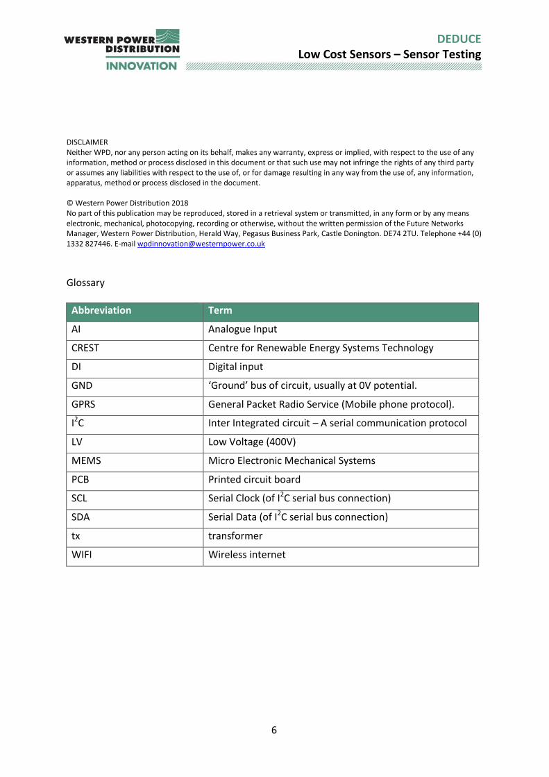
Glossary
Abbreviation Term
AI Analogue Input
CREST Centre for Renewable Energy Systems Technology
DI Digital input
GND ‘Ground’ bus of circuit, usually at 0V potential.
GPRS General Packet Radio Service (Mobile phone protocol).
I2C Inter Integrated circuit – A serial communication protocol
LV Low Voltage (400V)
MEMS Micro Electronic Mechanical Systems
PCB Printed circuit board
SCL Serial Clock (of I2C serial bus connection)
SDA Serial Data (of I2C serial bus connection)
tx transformer
WIFI Wireless internet
7
DEDUCE Low Cost Sensors – Sensor Testing
1 Executive Summary Recent growth in embedded generation such as wind and solar photovoltaic (PV) systems and the anticipated consumer uptake of electric vehicles (EVs) and heat pumps present new challenges for Western Power Distribution (WPD) to develop and operate its network which will experience greater fluctuation in electricity demand. Data from maximum demand indicators in distribution substations is inadequate to understand the spread of demand over time. Retro-fit datalogging solutions are available for substation monitoring, but cost typically >£1200, which would be difficult to justify for all WPDs 40,000 distribution substations. This NIA (Network Innovation Allowance) research project on network analogues is being conducted by CREST (Centre for Renewable Energy Systems Technology at Loughborough University in conjunction with WPD. The aim of the project is to identify and develop a novel low-cost monitoring approach with a target cost of £100 per substation. Engineering projects usually capture the requirements first then identify the best solutions for those requirements. This project intentionally has a tightly defined cost requirement and loose technical requirements, which are as follows:
The solution shall cost £100 or less excluding installation and operation costs.
The solution should give an indication of substation loading.
The solution should act as a replacement for existing MDIs (maximum demand indicator).
The solution should provide as many channels of useful data at the highest feasible resolution within the cost requirement.
The solution should consider how data will be transferred to a WPD datacentre or control room.
CREST have designed, built and coded 8 different sensors using three different control platforms. This document summarises the hardware requirements and laboratory testing against a set of pre-defined characteristics to determine usefulness and estimate value. High level results
The majority of the sensors and platforms for communication came within the target budget.
There were 3 sensors that could give a good indication of substation loading and 1 more where results were inconclusive.
There is capability to get at least 8 useable input/output channels on most platforms and many more on others.
The best resolution found was data logging to a server at an average of 7ms resolution using a Raspberry Pi. Typically 10s resolution was felt to be useful.
All the solutions can communicate via Wi-Fi or over the mobile Network (and in some cases through wired connection).
A summary of the key results is presented over.
8
DEDUCE Low Cost Sensors – Sensor Testing
Sensor Type Platform
Mag
net
om
eter
Hal
l Eff
ect
chip
I2m
co
il se
nso
r
Acc
eler
om
eter
Au
dio
Mic
rop
ho
ne
Stra
in g
auge
Ther
mal
sti
cker
s
Ther
mal
tra
nsd
uce
r
Low
co
st t
her
mal
imag
ing
An
dro
id P
ho
ne
Sen
sor
wit
h IO
IO
bo
ard
an
d p
ho
ne
Ard
uin
o
Ras
pb
erry
Pi
Cost £14 £2 £13 £19 £9 £31 £4 £99 £350 £13 + phone
£35 + phone
£49 £37
dongle
Application
Monitoring load close to real time < 10s
Load profiling (30min peak)
Exception reporting (> max value)
MDI ?
Data storage
Uploaded to a server ?
Stored locally
Data form
Current peak
Current RMS ?
1 phase
3 phase (cable)
Load from transformer ? ? ? ?
Data Quality
Linearity ? ? ?
Correlation with load > 0.999
>
0.996 0.34 0.48 -0.91 ? ?
> 0.999
Accuracy > 7.5%
>
10%1 ? ?
< 25%
? ? >
7.5%
Recommend for Field Trial
Tested, satisfactory > better than
Tested, unsuitable < worse than ? Test not conclusive 1There is still significant theory needed to back calculate current for distributed windings and this value could be easily improved.
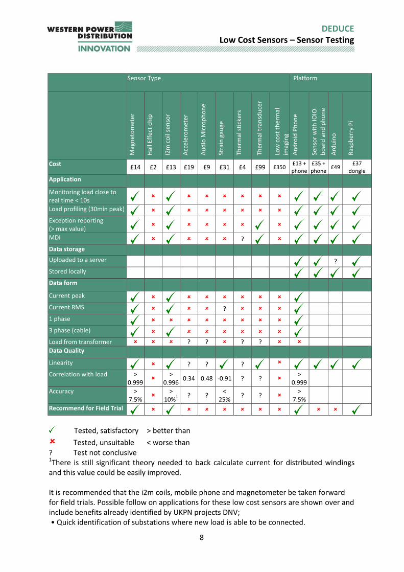
It is recommended that the i2m coils, mobile phone and magnetometer be taken forward for field trials. Possible follow on applications for these low cost sensors are shown over and include benefits already identified by UKPN projects DNV; • Quick identification of substations where new load is able to be connected.
9
DEDUCE Low Cost Sensors – Sensor Testing
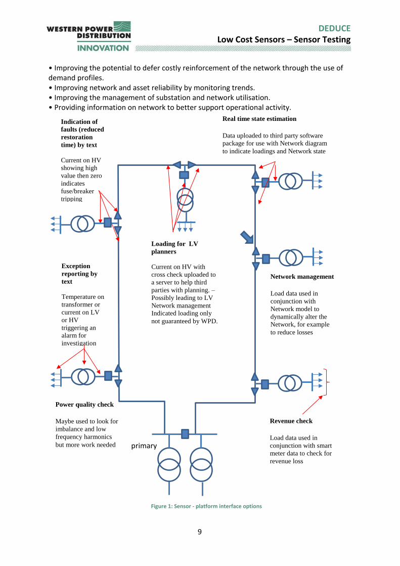
• Improving the potential to defer costly reinforcement of the network through the use of demand profiles. • Improving network and asset reliability by monitoring trends. • Improving the management of substation and network utilisation. • Providing information on network to better support operational activity.
Figure 1: Sensor - platform interface options
Exception
reporting by
text
Temperature on
transformer or
current on LV
or HV
triggering an
alarm for
investigation
Indication of
faults (reduced
restoration
time) by text Current on HV
showing high
value then zero
indicates
fuse/breaker
tripping
Loading for LV
planners
Current on HV with
cross check uploaded to
a server to help third
parties with planning. –
Possibly leading to LV
Network management
Indicated loading only
not guaranteed by WPD.
Real time state estimation
Data uploaded to third party software
package for use with Network diagram
to indicate loadings and Network state
Network management Load data used in
conjunction with
Network model to
dynamically alter the
Network, for example
to reduce losses
Revenue check Load data used in
conjunction with smart
meter data to check for
revenue loss
primary
Power quality check Maybe used to look for
imbalance and low
frequency harmonics
but more work needed

10
DEDUCE Low Cost Sensors – Sensor Testing
2 Introduction
2.1 Background DNOs currently have very limited visibility of LV networks. With Supervisory Control And Data Acquisition (SCADA) systems generally limited to 11kV feeders, visibility of LV network loading is restricted to Maximum Demand Indicators (MDI). These manual readings are generally supplemented with industry metering flows to develop an understanding of network loading. MDIs are restricted by their need to be reset periodically as well as the potential for network back-feeds to distort readings. Several previous LCNF projects have investigated LV monitoring. This has pushed the market for LV monitoring forward significantly from the custom-built units used for the Low Voltage Network Templates project, to several commercially available units available to date. WPD currently has Standard Techniques (STs) for the installation of ground mounted and overhead monitoring as well as a fully tendered framework agreement for the supply of such units. These units depend primarily on the measurement of voltage and current to determine loading. Voltage is generally measured directly using busbar clamps or modified fuse holders with a voltage take off point. Current is generally measured using Rogowski coils. These units can measure the detailed loading of each phase on each feeder and provide a significant level of detail and granularity. However, these devices are also costly due to the requirement for multiple sensors. This has limited their roll out to date. This project looks to develop a low cost (sub £100) distribution substation monitor based on indirect loading measures (for example; magnetic field, temperature, noise and vibration). At a minimum this must give access to more granular and less error prone data than is currently acquired through MDIs. The substation monitor is expected to develop a methodology for the acquisition of basic whole substation loading profiles as well as the optimal method for the delivery of such data to planning teams and simplicity of installation. To meet these aims the following approaches are proposed:
To investigate existing low-cost sensors that can be used for indirect substation loading monitoring.
To investigate new disruptive technologies to determine their suitability and accuracy for monitoring
To use existing low-cost measurement devices or packages (such as a smart phone or raspberry pi) to indirectly provide measurement
To run a university-based competition to enable non-traditional solutions to be explored Several different sensors technologies were identified in the review document. These have now been designed, built and tested. The designs went through an iterative procedure as improvements were identified as part of testing and lessons learned were captured. This
11
DEDUCE Low Cost Sensors – Sensor Testing
document contains the “as built” hardware details of the sensors that have been manufactured prior to testing, the changes to hardware as testing has progressed and a summary of that testing.
2.2 Scope The project is aimed at 11kV:400kV 50Hz distribution substations connected to public distribution networks. The project focuses on ground mounted substations on the 11kV distribution network since these account for the bulk of final LV demand. As such pole mounted transformers and substations on legacy 6.6kV networks are not specifically covered since they are a small proportion of overall demand. Likewise, primary substations are not specifically considered since the smaller number of primaries and greater power flow means more accurate and robust solutions are more like to be justified economically. Monitoring at the DNO/meter operator/consumer interface is not considered since a wide range of parameters will be available from smart meters as they are commissioned as part of a national program. The findings of this project may have relevance for monitoring of pole mounted transformers, 6.6kV substations and primary substations which could be determined as part of a successor project.
2.3 Presentation of learning Throughout the document, key learning outcomes are presented in a box as follows:
LP x Brief description of learning.
Each piece of project feedback is referenced as a uniquely numbered Learning Point (LP). All learning points are collected together in Appendix A. In addition there are a set of technical tips which contain technical pointers for anyone looking to replicate this work
TT x Brief description of a technical tip for anyone trying to replicate this work
12
DEDUCE Low Cost Sensors – Sensor Testing
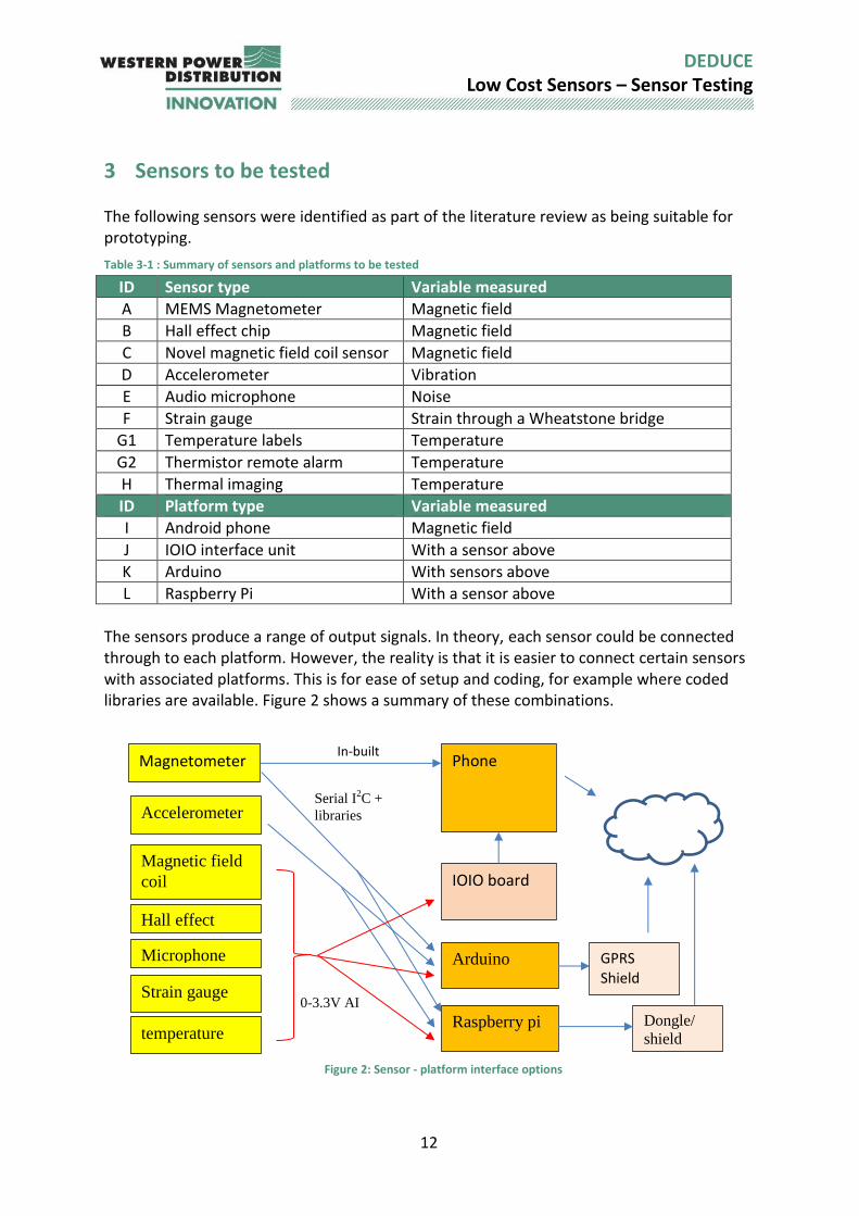
3 Sensors to be tested The following sensors were identified as part of the literature review as being suitable for prototyping.
Table 3-1 : Summary of sensors and platforms to be tested
ID Sensor type Variable measured
A MEMS Magnetometer Magnetic field
B Hall effect chip Magnetic field
C Novel magnetic field coil sensor Magnetic field
D Accelerometer Vibration
E Audio microphone Noise
F Strain gauge Strain through a Wheatstone bridge
G1 Temperature labels Temperature
G2 Thermistor remote alarm Temperature
H Thermal imaging Temperature
ID Platform type Variable measured
I Android phone Magnetic field
J IOIO interface unit With a sensor above
K Arduino With sensors above
L Raspberry Pi With a sensor above
The sensors produce a range of output signals. In theory, each sensor could be connected through to each platform. However, the reality is that it is easier to connect certain sensors with associated platforms. This is for ease of setup and coding, for example where coded libraries are available. Figure 2 shows a summary of these combinations.
Figure 2: Sensor - platform interface options
Magnetometer Phone In-built
Accelerometer
IOIO board
Arduino
Raspberry pi
GPRS Shield
Dongle/
shield
Magnetic field
coil
Hall effect
Microphone
Strain gauge
temperature
Serial I2C +
libraries
0-3.3V AI
13
DEDUCE Low Cost Sensors – Sensor Testing
Not all the sensors can measure loading on all types of cable. Usually, sensors only measure single core or three core cable types.
LP 1 Sensors to measure current in multicore/trefoil cables are not commercially available and there is no available published literature on measurement solutions. These are the most popular type of cable on the Distribution Network. Therefore, measuring these types of cable without separating the cores with a single sensor may be valuable.
Section 4 looks at the testing facilities while section 5 onwards considers each sensor and the platform in turn. Each section includes details about the hardware, parts list and its cost, how each sensor is set up ready for testing, followed by test results where applicable. Where the sensor looks a promising candidate for taking forward to field trial the theory behind the back calculation of current is also included.
14
DEDUCE Low Cost Sensors – Sensor Testing
4 Electrical test facilities at CREST.
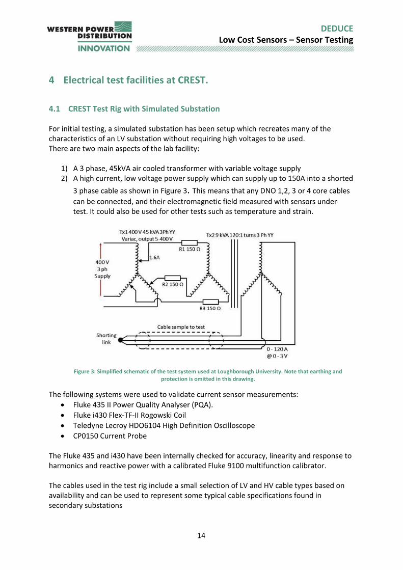
4.1 CREST Test Rig with Simulated Substation For initial testing, a simulated substation has been setup which recreates many of the characteristics of an LV substation without requiring high voltages to be used. There are two main aspects of the lab facility:
1) A 3 phase, 45kVA air cooled transformer with variable voltage supply 2) A high current, low voltage power supply which can supply up to 150A into a shorted
3 phase cable as shown in Figure 3. This means that any DNO 1,2, 3 or 4 core cables
can be connected, and their electromagnetic field measured with sensors under test. It could also be used for other tests such as temperature and strain.
Figure 3: Simplified schematic of the test system used at Loughborough University. Note that earthing and
protection is omitted in this drawing.
The following systems were used to validate current sensor measurements:
Fluke 435 II Power Quality Analyser (PQA).
Fluke i430 Flex-TF-II Rogowski Coil
Teledyne Lecroy HDO6104 High Definition Oscilloscope
CP0150 Current Probe
The Fluke 435 and i430 have been internally checked for accuracy, linearity and response to harmonics and reactive power with a calibrated Fluke 9100 multifunction calibrator. The cables used in the test rig include a small selection of LV and HV cable types based on availability and can be used to represent some typical cable specifications found in secondary substations
15
DEDUCE Low Cost Sensors – Sensor Testing
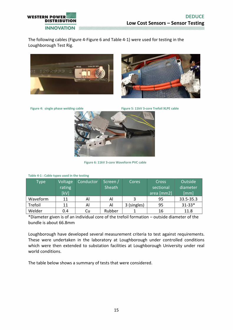
The following cables (Figure 4-Figure 6 and Table 4-1) were used for testing in the Loughborough Test Rig.
Figure 4: single phase welding cable Figure 5: 11kV 3-core Trefoil XLPE cable
Figure 6: 11kV 3-core Waveform PVC cable
Table 4-1 : Cable types used in the testing
Type Voltage rating [kV]
Conductor Screen / Sheath
Cores Cross sectional
area [mm2]
Outside diameter
[mm]
Waveform 11 Al Al 3 95 33.5-35.3
Trefoil 11 Al Al 3 (singles) 95 31-33*
Welder 0.4 Cu Rubber 1 16 11.8
*Diameter given is of an individual core of the trefoil formation – outside diameter of the bundle is about 66.8mm Loughborough have developed several measurement criteria to test against requirements. These were undertaken in the laboratory at Loughborough under controlled conditions which were then extended to substation facilities at Loughborough University under real world conditions. The table below shows a summary of tests that were considered.
16
DEDUCE Low Cost Sensors – Sensor Testing
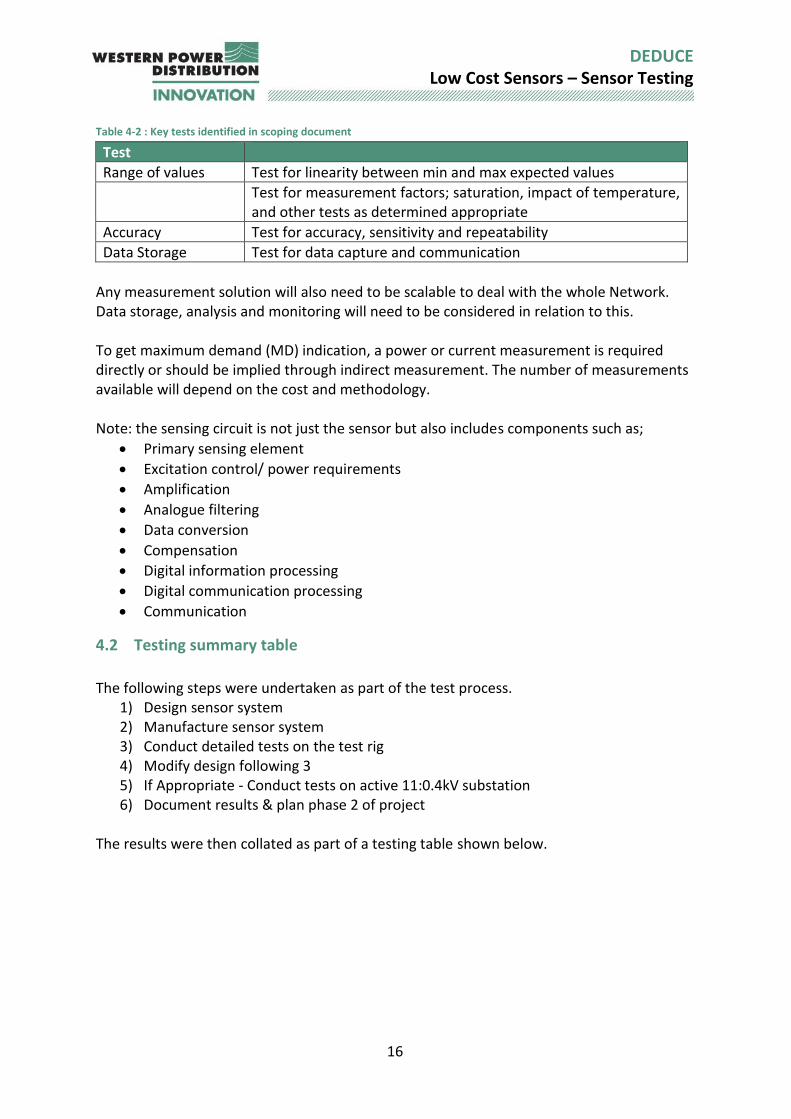
Table 4-2 : Key tests identified in scoping document
Test
Range of values Test for linearity between min and max expected values
Test for measurement factors; saturation, impact of temperature, and other tests as determined appropriate
Accuracy Test for accuracy, sensitivity and repeatability
Data Storage Test for data capture and communication
Any measurement solution will also need to be scalable to deal with the whole Network. Data storage, analysis and monitoring will need to be considered in relation to this. To get maximum demand (MD) indication, a power or current measurement is required directly or should be implied through indirect measurement. The number of measurements available will depend on the cost and methodology. Note: the sensing circuit is not just the sensor but also includes components such as;
Primary sensing element
Excitation control/ power requirements
Amplification
Analogue filtering
Data conversion
Compensation
Digital information processing
Digital communication processing
Communication
4.2 Testing summary table
The following steps were undertaken as part of the test process.
1) Design sensor system 2) Manufacture sensor system 3) Conduct detailed tests on the test rig 4) Modify design following 3 5) If Appropriate - Conduct tests on active 11:0.4kV substation 6) Document results & plan phase 2 of project
The results were then collated as part of a testing table shown below.
17
DEDUCE Low Cost Sensors – Sensor Testing
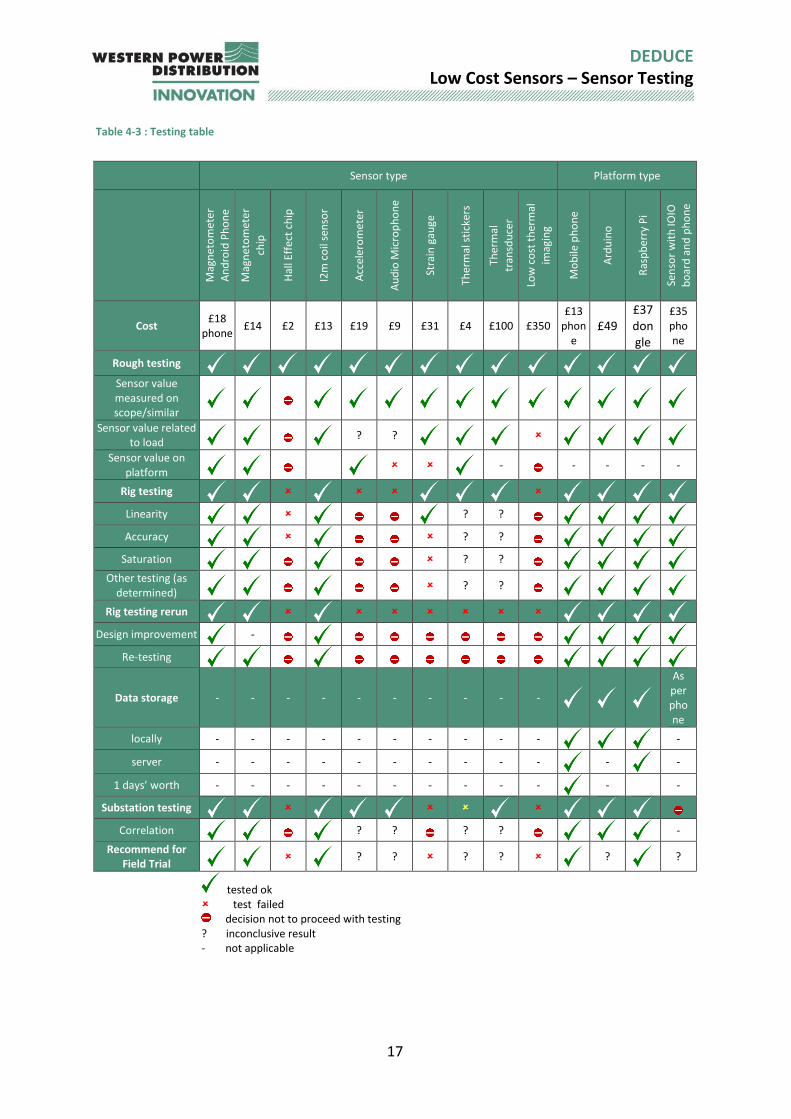
Table 4-3 : Testing table
Sensor type Platform type
Mag
net
om
ete
r
An
dro
id P
ho
ne
Mag
net
om
ete
r
chip
Hal
l Eff
ect
chip
I2m
co
il se
nso
r
Acc
eler
om
eter
Au
dio
Mic
rop
ho
ne
Stra
in g
auge
Ther
mal
sti
cker
s
Ther
mal
tran
sdu
cer
Low
co
st t
her
mal
imag
ing
Mo
bile
ph
on
e
Ard
uin
o
Ras
pb
erry
Pi
Sen
sor
wit
h IO
IO
bo
ard
an
d p
ho
ne
Cost £18
phone £14 £2 £13 £19 £9 £31 £4 £100 £350
£13 phon
e £49
£37 dongle
£35 phone
Rough testing
Sensor value measured on scope/similar
Sensor value related to load
? ?
Sensor value on platform
- - - - -
Rig testing
Linearity
? ?
Accuracy
? ?
Saturation ? ?
Other testing (as determined) ? ?
Rig testing rerun
Design improvement
-
Re-testing
Data storage - - - - - - - - - -
As per phone
locally - - - - - - - - - -
-
server - - - - - - - - - -
-
-
1 days’ worth - - - - - - - - - -
- -
Substation testing
Correlation
? ? ? ? -
Recommend for Field Trial
? ? ? ?
?
?
tested ok test failed decision not to proceed with testing ? inconclusive result - not applicable
18
DEDUCE Low Cost Sensors – Sensor Testing
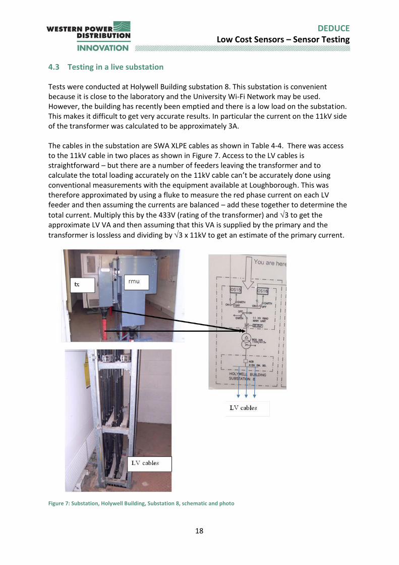
4.3 Testing in a live substation Tests were conducted at Holywell Building substation 8. This substation is convenient because it is close to the laboratory and the University Wi-Fi Network may be used. However, the building has recently been emptied and there is a low load on the substation. This makes it difficult to get very accurate results. In particular the current on the 11kV side of the transformer was calculated to be approximately 3A. The cables in the substation are SWA XLPE cables as shown in Table 4-4. There was access to the 11kV cable in two places as shown in Figure 7. Access to the LV cables is straightforward – but there are a number of feeders leaving the transformer and to calculate the total loading accurately on the 11kV cable can’t be accurately done using conventional measurements with the equipment available at Loughborough. This was therefore approximated by using a fluke to measure the red phase current on each LV feeder and then assuming the currents are balanced – add these together to determine the
total current. Multiply this by the 433V (rating of the transformer) and 3 to get the approximate LV VA and then assuming that this VA is supplied by the primary and the
transformer is lossless and dividing by 3 x 11kV to get an estimate of the primary current.
Figure 7: Substation, Holywell Building, Substation 8, schematic and photo
19
DEDUCE Low Cost Sensors – Sensor Testing
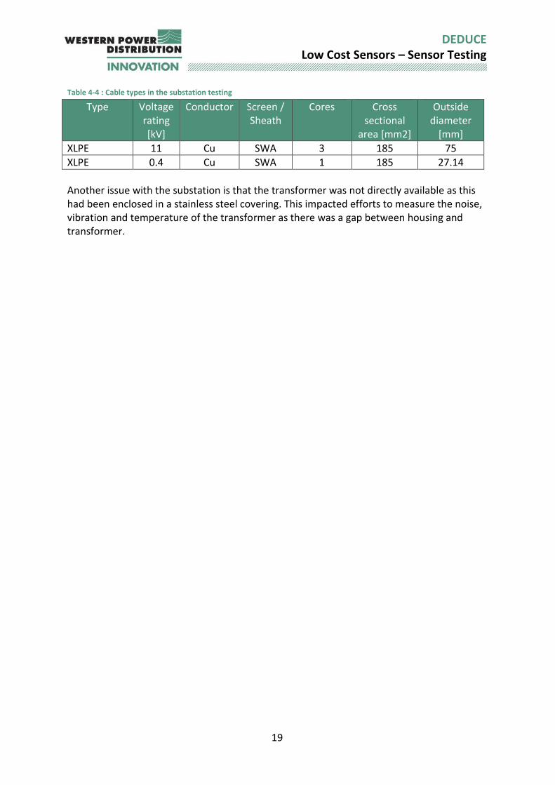
Table 4-4 : Cable types in the substation testing
Type Voltage rating [kV]
Conductor Screen / Sheath
Cores Cross sectional
area [mm2]
Outside diameter
[mm]
XLPE 11 Cu SWA 3 185 75
XLPE 0.4 Cu SWA 1 185 27.14
Another issue with the substation is that the transformer was not directly available as this had been enclosed in a stainless steel covering. This impacted efforts to measure the noise, vibration and temperature of the transformer as there was a gap between housing and transformer.
20
DEDUCE Low Cost Sensors – Sensor Testing
5 Sensor A: MEMS Magnetometer
5.1 Theory
A magnetometer measures magnetic field in three directions (x,y and z). Typically these
are in T. The relationship between current and magnetic field comes from Amperes law. The magnetic flux density B (T) at a distance r (m) from the centre of a conductor can be calculated from Equation 5-1.
𝐵 = 𝜇𝐼
2𝜋𝑟 Equation 5-1
Where 𝐼 is the current in the conductor (A) and 𝜇 = 𝜇𝑟𝜇𝑜 is the magnetic permeability
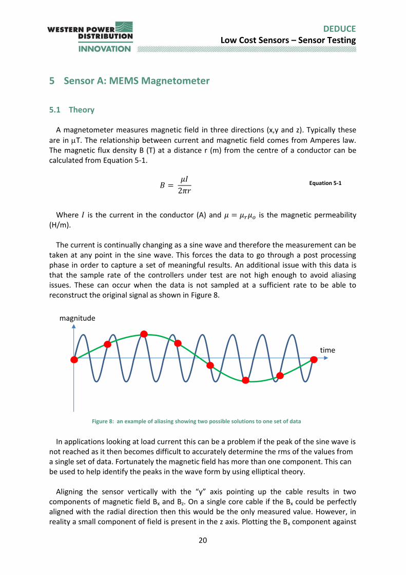
(H/m). The current is continually changing as a sine wave and therefore the measurement can be
taken at any point in the sine wave. This forces the data to go through a post processing phase in order to capture a set of meaningful results. An additional issue with this data is that the sample rate of the controllers under test are not high enough to avoid aliasing issues. These can occur when the data is not sampled at a sufficient rate to be able to reconstruct the original signal as shown in Figure 8.
Figure 8: an example of aliasing showing two possible solutions to one set of data
In applications looking at load current this can be a problem if the peak of the sine wave is
not reached as it then becomes difficult to accurately determine the rms of the values from a single set of data. Fortunately the magnetic field has more than one component. This can be used to help identify the peaks in the wave form by using elliptical theory.
Aligning the sensor vertically with the “y” axis pointing up the cable results in two components of magnetic field Bx and Bz. On a single core cable if the Bx could be perfectly aligned with the radial direction then this would be the only measured value. However, in reality a small component of field is present in the z axis. Plotting the Bx component against
magnitude
time
21
DEDUCE Low Cost Sensors – Sensor Testing
the Bz component traces out an ellipse which may be offset (for example by the Earth’s magnetic field) as shown in Figure 9. If the magnetic field due to the current can be measured then the current can be back calculated. The magnetic flux density related to the presence of a single core cables can consider only a single current assuming no other cables are close by. However, the field produced by multi-core cables needs to consider the impact of the current in all the phases on the flux density. The solution is to use Principle component analysis.
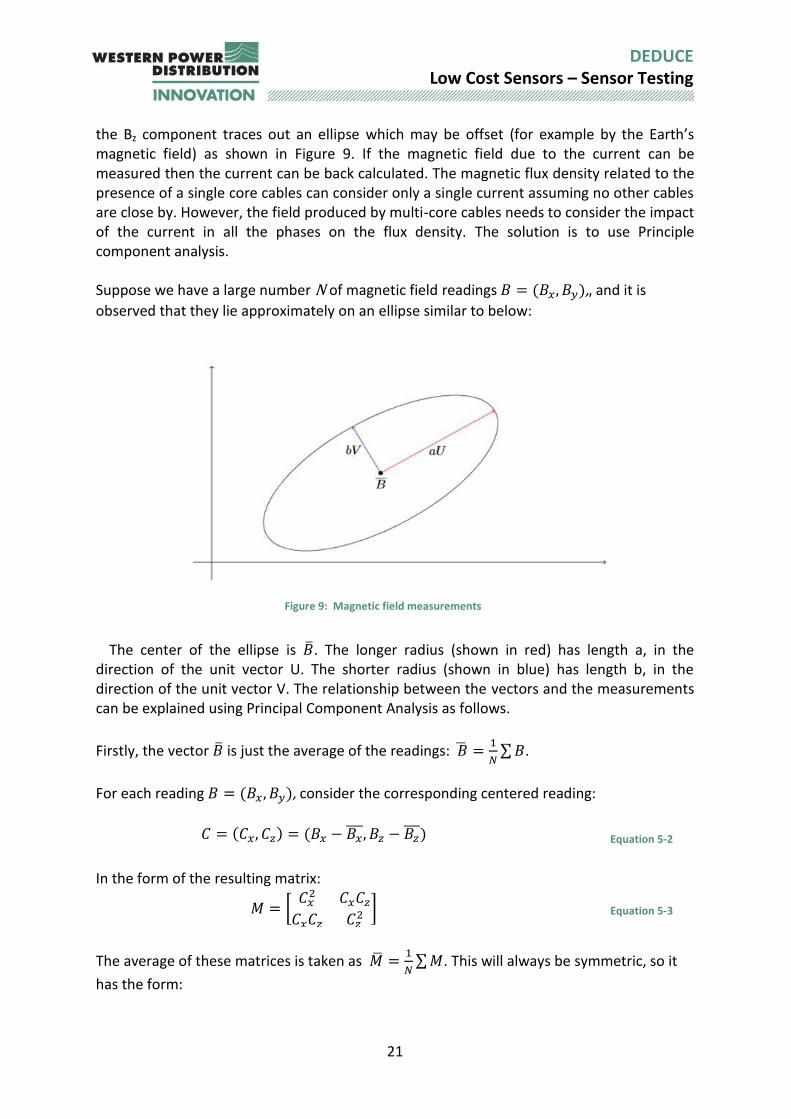
Suppose we have a large number N of magnetic field readings 𝐵 = (𝐵𝑥, 𝐵𝑦),, and it is
observed that they lie approximately on an ellipse similar to below:
Figure 9: Magnetic field measurements
The center of the ellipse is ��. The longer radius (shown in red) has length a, in the
direction of the unit vector U. The shorter radius (shown in blue) has length b, in the direction of the unit vector V. The relationship between the vectors and the measurements can be explained using Principal Component Analysis as follows.
Firstly, the vector �� is just the average of the readings: �� =1
𝑁∑ 𝐵.
For each reading 𝐵 = (𝐵𝑥, 𝐵𝑦), consider the corresponding centered reading:
𝐶 = (𝐶𝑥, 𝐶𝑧) = (𝐵𝑥 − 𝐵𝑥
, 𝐵𝑧 − 𝐵𝑧 ) Equation 5-2
In the form of the resulting matrix:
𝑀 = [𝐶𝑥
2 𝐶𝑥𝐶𝑧
𝐶𝑥𝐶𝑧 𝐶𝑧2 ] Equation 5-3
The average of these matrices is taken as �� =1
𝑁∑ 𝑀. This will always be symmetric, so it
has the form:
22
DEDUCE Low Cost Sensors – Sensor Testing
�� = [𝑃 𝑄𝑄 𝑅
] Equation 5-4
for some P, Q, R.
Putting S= (P−R)2+4Q2. The lengths of the two elipse radii 𝑎 and 𝑏 are
𝑎 = √𝑃 + 𝑅 + 𝑆 Equation 5-5
And
𝑏 = √𝑃 + 𝑅 − 𝑆 Equation 5-6
The unit vectors U and V can be found as
𝑈 = (2𝑄, 𝑅 − 𝑃 + 𝑆) /√4𝑄2 + (𝑅 − 𝑃 + 𝑆)2 Equation 5-7
𝑉 = (2𝑄, 𝑅 − 𝑃 − 𝑆) /√4𝑄2 + (𝑅 − 𝑃 − 𝑆)2 Equation 5-8
Alternatively, U and V are the eigenvectors of ��, with eigenvalues 𝑎2/2 and 𝑏2/2. It is also useful to consider the matrix
𝑇 = [𝑈𝑥/𝑎 𝑈𝑧/𝑎𝑉𝑥/𝑏 𝑉𝑧/𝑏
] Equation 5-9
For each centered reading C, the vector TC should lie on the unit circle, so we should have |TC |=1. In practice the original readings will not lie exactly on an ellipse so |TC | will not be exactly equal to 1. As the data is a continuous stream and the sampling period of the phone is asynchronous it is necessary to consider how the data is analysed and reported back to the user. In this project a faded average or exponential moving average (EMA) method was implemented as follows. Consider a set of readings 𝑥1, 𝑥2, 𝑥3 … . . 𝑥𝑛
The average of these readings is �� =1
𝑛(𝑥1 + 𝑥2 + 𝑥3, … . . 𝑥𝑛)
The EMA is defined as
𝑥𝑒𝑥𝑝 =𝑥𝑛 + 𝜃𝑥𝑛−1 + 𝜃2𝑥𝑛−2 + ⋯
1 + 𝜃 + 𝜃2 + ⋯ Equation 5-10
For some 𝜃 = 𝑒−𝜏 where is small and positive so ≈1 and equal to δt/k where δt is the change in time and k a constant. Adding a new reading 𝑥𝑛+1 the new exponential moving average becomes
𝑥𝑒𝑥𝑝,𝑛𝑒𝑤 = 𝜃𝑥𝑒𝑥𝑝,𝑜𝑙𝑑 + (1 − 𝜃)𝑥𝑛+1 Equation 5-11
23
DEDUCE Low Cost Sensors – Sensor Testing
This equation is computationally efficient, since it doesn’t require a set or previous measurements to be stored in memory only the most recent raw measurement and the EMA calculated for the previous measurement. Once the magnetic flux density is determined then the peak load current can be calculated. This is straightforward for a single core cable as
𝐼 = 2𝜋𝑟��
𝜇 Equation 5-12
Where �� is the equivalent to “a” in Equation 5-5.
The measurement distance r, is taken as the estimated distance of the sensor location to the center of the conductor. This therefore varies with each installation as cable diameter changes depending on the substation design. This is also dependent on the location of the sensor and whether or not it is in a phone. If it is contained in the phone then this also changes with phone type.
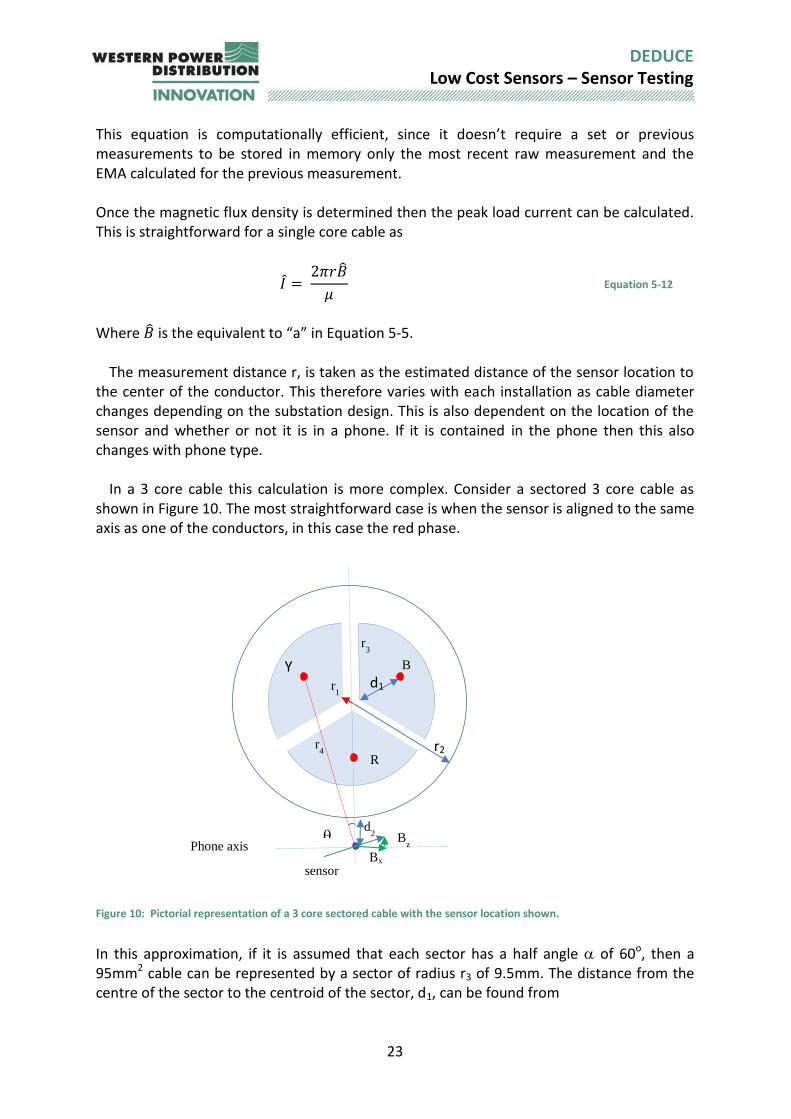
In a 3 core cable this calculation is more complex. Consider a sectored 3 core cable as shown in Figure 10. The most straightforward case is when the sensor is aligned to the same axis as one of the conductors, in this case the red phase.
Figure 10: Pictorial representation of a 3 core sectored cable with the sensor location shown.
In this approximation, if it is assumed that each sector has a half angle of 60o, then a 95mm2 cable can be represented by a sector of radius r3 of 9.5mm. The distance from the centre of the sector to the centroid of the sector, d1, can be found from
Phone axis
Y d1
r2
r1
R
B
sensor
r4
r3
d2
Bx
Bz
24
DEDUCE Low Cost Sensors – Sensor Testing
𝑑1 =2𝑟3sin (𝛼)
3𝛼
Equation 5-13
The field at the sensor due to the current in conductor R can be assumed to be in the x direction only and can be calculated from:
𝐵𝑥 =𝜇𝑜𝐼𝑠𝑖𝑛(𝜔𝑡)
2𝜋(𝑑2 + 𝑟2 − 𝑑1 − 𝑟1)=
𝜇𝑜𝐼𝑠𝑖𝑛(𝜔𝑡)
2𝜋𝑑3
Equation 5-14
The distance from the centre of conductor Y and B to the sensor is then found from
𝑟4 = √(𝑟2 + 𝑑2)2 + (𝑟1 + 𝑑1)2 + (𝑟2 + 𝑑2)(𝑟1 + 𝑑1)
Equation 5-15
The magnetic flux density at the sensor due to the current in conductor Y,
𝐼𝑌 = 𝐼sin (𝜔𝑡 − 120𝑜) is given by Equation 5-16 and Equation 5-17.
𝐵𝑥 =𝜇𝑜𝐼𝑠𝑖𝑛(𝜔𝑡 − 2𝜋/3) cos (𝜃)
2𝜋𝑟4
Equation 5-16
𝐵𝑧 = −𝜇𝑜𝐼𝑠𝑖𝑛(𝜔𝑡 − 2𝜋/3)sin (𝜃)
2𝜋𝑟4
Equation 5-17
Where sin(𝜃) =√3(𝑑1+𝑟1)
2𝑟4.
A similar equation for the field at the sensor due to the current in the B conductor can also be calculated If it is assumed that the currents in all three phases are balanced then the peak flux density can be related back to the peak current through Equation 5-18.
𝐼 =2𝜋��
𝑔𝑓𝜇𝑜
Equation 5-18
Where gf is a geometric factor relating to the back calculation and is equal to:
𝑔𝑓 =1
𝑑3
−cos (𝜃)
𝑟4
Equation 5-19
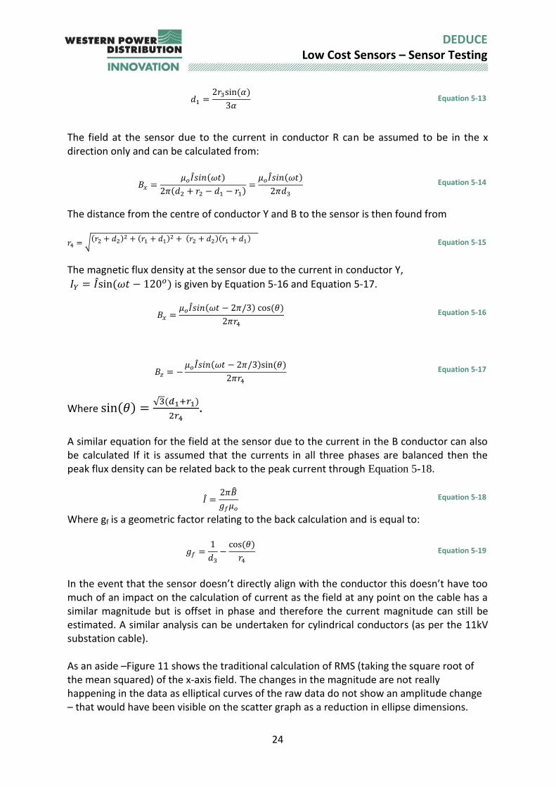
In the event that the sensor doesn’t directly align with the conductor this doesn’t have too much of an impact on the calculation of current as the field at any point on the cable has a similar magnitude but is offset in phase and therefore the current magnitude can still be estimated. A similar analysis can be undertaken for cylindrical conductors (as per the 11kV substation cable). As an aside –Figure 11 shows the traditional calculation of RMS (taking the square root of the mean squared) of the x-axis field. The changes in the magnitude are not really happening in the data as elliptical curves of the raw data do not show an amplitude change – that would have been visible on the scatter graph as a reduction in ellipse dimensions.
25
DEDUCE Low Cost Sensors – Sensor Testing
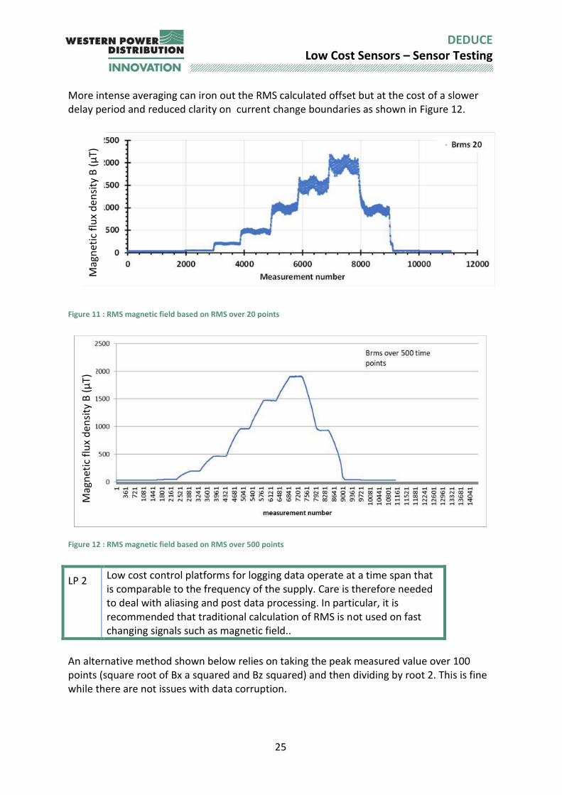
More intense averaging can iron out the RMS calculated offset but at the cost of a slower delay period and reduced clarity on current change boundaries as shown in Figure 12.
Figure 11 : RMS magnetic field based on RMS over 20 points
Figure 12 : RMS magnetic field based on RMS over 500 points
LP 2 Low cost control platforms for logging data operate at a time span that is comparable to the frequency of the supply. Care is therefore needed to deal with aliasing and post data processing. In particular, it is recommended that traditional calculation of RMS is not used on fast changing signals such as magnetic field..
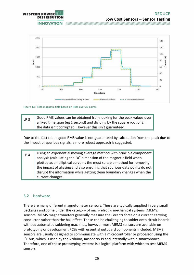
An alternative method shown below relies on taking the peak measured value over 100 points (square root of Bx a squared and Bz squared) and then dividing by root 2. This is fine while there are not issues with data corruption.
Mag
net
ic f
lux
de
nsi
ty B
(μ
T)
Mag
net
ic f
lux
den
sity
B (
μT)
26
DEDUCE Low Cost Sensors – Sensor Testing
Figure 13 : RMS magnetic field based on RMS over 20 points
LP 3 Good RMS values can be obtained from looking for the peak values over a fixed time span (eg 1 second) and dividing by the square root of 2 if the data isn’t corrupted. However this isn’t guaranteed.
Due to the fact that a good RMS value is not guaranteed by calculation from the peak due to the impact of spurious signals, a more robust approach is suggested.
LP 4 Using an exponential moving average method with principle component analysis (calculating the “a” dimension of the magnetic field when plotted as an elliptical curve) is the most suitable method for removing the impact of aliasing and also ensuring that spurious data points do not disrupt the information while getting clean boundary changes when the current changes.
5.2 Hardware There are many different magnetometer sensors. These are typically supplied in very small packages and come under the category of micro electro mechanical systems (MEMS) sensors. MEMS magnetometers generally measure the Lorentz force on a current carrying conductor rather than the hall effect. These can be challenging to solder onto circuit boards without automated soldering machines, however most MEMS sensors are available on prototyping or development PCBs with essential outboard components included. MEMS sensors are usually designed to communicate with a microcontroller or processor using the I2C bus, which is used by the Arduino, Raspberry Pi and internally within smartphones. Therefore, one of these prototyping systems is a logical platform with which to test MEMS sensors.
27
DEDUCE Low Cost Sensors – Sensor Testing
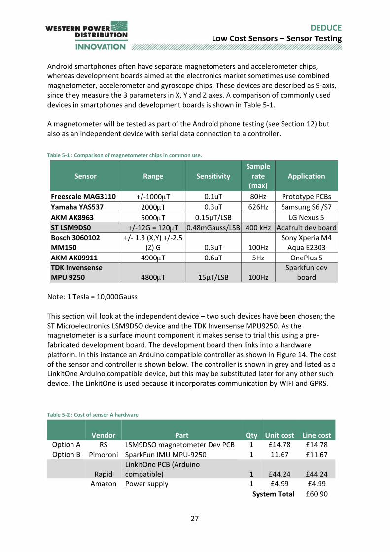
Android smartphones often have separate magnetometers and accelerometer chips, whereas development boards aimed at the electronics market sometimes use combined magnetometer, accelerometer and gyroscope chips. These devices are described as 9-axis, since they measure the 3 parameters in X, Y and Z axes. A comparison of commonly used devices in smartphones and development boards is shown in Table 5-1. A magnetometer will be tested as part of the Android phone testing (see Section 12) but also as an independent device with serial data connection to a controller.
Table 5-1 : Comparison of magnetometer chips in common use.
Sensor Range Sensitivity Sample
rate (max)
Application
Freescale MAG3110 +/-1000T 0.1uT 80Hz Prototype PCBs
Yamaha YAS537 2000T 0.3uT 626Hz Samsung S6 /S7
AKM AK8963 5000T 0.15μT/LSB
LG Nexus 5
ST LSM9DS0 +/-12G = 120T 0.48mGauss/LSB 400 kHz Adafruit dev board
Bosch 3060102 MM150
+/- 1.3 (X,Y) +/-2.5 (Z) G 0.3uT 100Hz
Sony Xperia M4 Aqua E2303
AKM AK09911 4900T 0.6uT 5Hz OnePlus 5
TDK Invensense MPU 9250 4800T 15μT/LSB 100Hz
Sparkfun dev board
Note: 1 Tesla = 10,000Gauss This section will look at the independent device – two such devices have been chosen; the ST Microelectronics LSM9DSO device and the TDK Invensense MPU9250. As the magnetometer is a surface mount component it makes sense to trial this using a pre-fabricated development board. The development board then links into a hardware platform. In this instance an Arduino compatible controller as shown in Figure 14. The cost of the sensor and controller is shown below. The controller is shown in grey and listed as a LinkitOne Arduino compatible device, but this may be substituted later for any other such device. The LinkitOne is used because it incorporates communication by WIFI and GPRS.
Table 5-2 : Cost of sensor A hardware
Vendor Part Qty Unit cost Line cost Option A RS LSM9DSO magnetometer Dev PCB 1 £14.78 £14.78 Option B Pimoroni SparkFun IMU MPU-9250 1 11.67 £11.67
Rapid
LinkitOne PCB (Arduino compatible) 1 £44.24 £44.24
Amazon Power supply 1 £4.99 £4.99
System Total £60.90
28
DEDUCE Low Cost Sensors – Sensor Testing
Figure 14: Photo of Arduino Uno with LSM9DSO magnetometer circuit
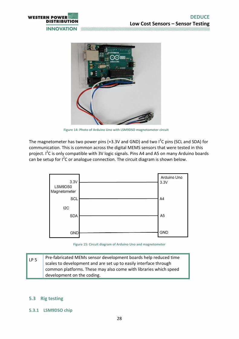
The magnetometer has two power pins (+3.3V and GND) and two I2C pins (SCL and SDA) for communication. This is common across the digital MEMS sensors that were tested in this project. I2C is only compatible with 3V logic signals. Pins A4 and A5 on many Arduino boards can be setup for I2C or analogue connection. The circuit diagram is shown below.
Figure 15: Circuit diagram of Arduino Uno and magnetometer
LP 5 Pre-fabricated MEMs sensor development boards help reduced time scales to development and are set up to easily interface through common platforms. These may also come with libraries which speed development on the coding.
5.3 Rig testing 5.3.1 LSM9DSO chip
29
DEDUCE Low Cost Sensors – Sensor Testing
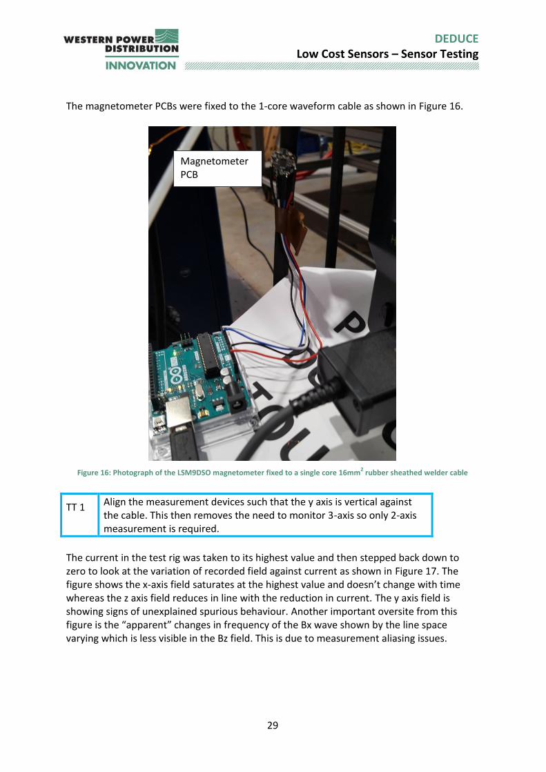
The magnetometer PCBs were fixed to the 1-core waveform cable as shown in Figure 16.
Figure 16: Photograph of the LSM9DSO magnetometer fixed to a single core 16mm
2 rubber sheathed welder cable
TT 1 Align the measurement devices such that the y axis is vertical against the cable. This then removes the need to monitor 3-axis so only 2-axis measurement is required.
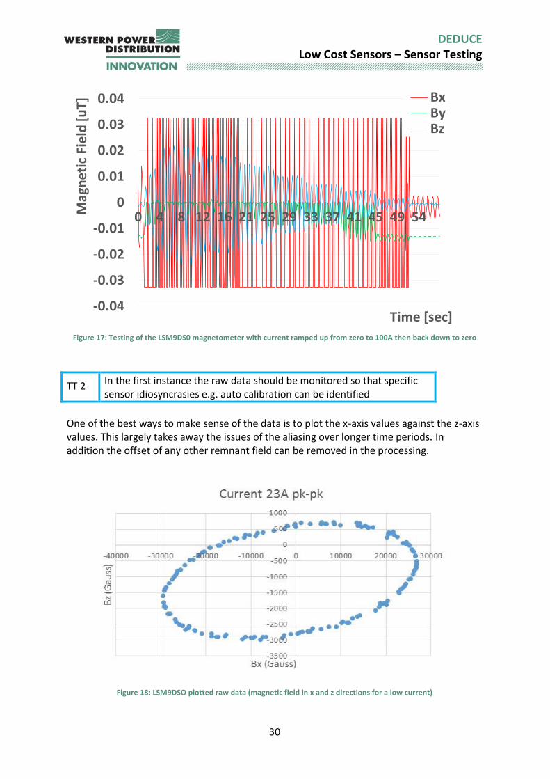
The current in the test rig was taken to its highest value and then stepped back down to zero to look at the variation of recorded field against current as shown in Figure 17. The figure shows the x-axis field saturates at the highest value and doesn’t change with time whereas the z axis field reduces in line with the reduction in current. The y axis field is showing signs of unexplained spurious behaviour. Another important oversite from this figure is the “apparent” changes in frequency of the Bx wave shown by the line space varying which is less visible in the Bz field. This is due to measurement aliasing issues.
Magnetometer PCB
30
DEDUCE Low Cost Sensors – Sensor Testing
Figure 17: Testing of the LSM9DS0 magnetometer with current ramped up from zero to 100A then back down to zero
TT 2 In the first instance the raw data should be monitored so that specific sensor idiosyncrasies e.g. auto calibration can be identified
One of the best ways to make sense of the data is to plot the x-axis values against the z-axis values. This largely takes away the issues of the aliasing over longer time periods. In addition the offset of any other remnant field can be removed in the processing.
Figure 18: LSM9DSO plotted raw data (magnetic field in x and z directions for a low current)
-0.04
-0.03
-0.02
-0.01
0
0.01
0.02
0.03
0.04
0 4 8 12 16 21 25 29 33 37 41 45 49 54Mag
net
ic F
ield
[uT]
Time [sec]
BxByBz
31
DEDUCE Low Cost Sensors – Sensor Testing
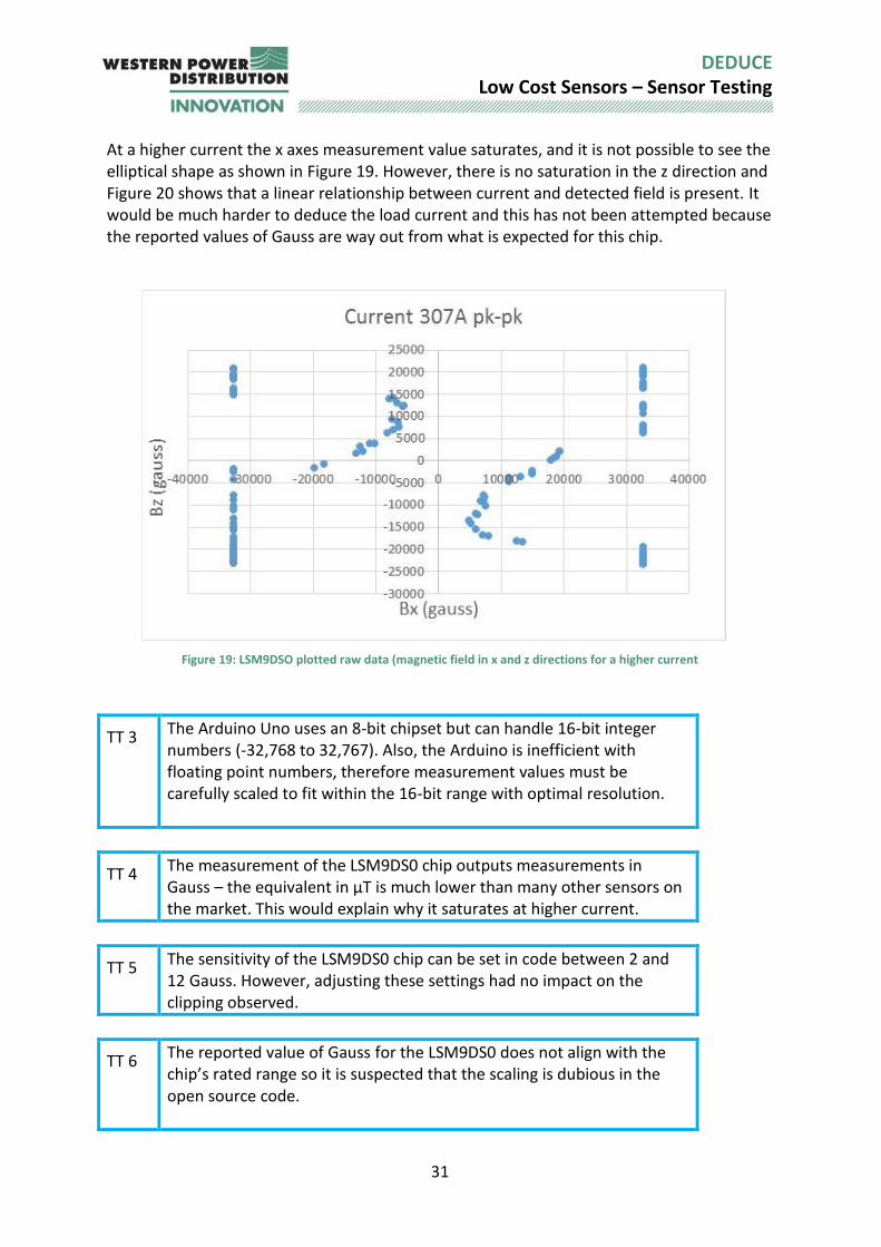
At a higher current the x axes measurement value saturates, and it is not possible to see the elliptical shape as shown in Figure 19. However, there is no saturation in the z direction and Figure 20 shows that a linear relationship between current and detected field is present. It would be much harder to deduce the load current and this has not been attempted because the reported values of Gauss are way out from what is expected for this chip.
Figure 19: LSM9DSO plotted raw data (magnetic field in x and z directions for a higher current
TT 3 The Arduino Uno uses an 8-bit chipset but can handle 16-bit integer numbers (-32,768 to 32,767). Also, the Arduino is inefficient with floating point numbers, therefore measurement values must be carefully scaled to fit within the 16-bit range with optimal resolution.
TT 4 The measurement of the LSM9DS0 chip outputs measurements in Gauss – the equivalent in μT is much lower than many other sensors on the market. This would explain why it saturates at higher current.
TT 5 The sensitivity of the LSM9DS0 chip can be set in code between 2 and 12 Gauss. However, adjusting these settings had no impact on the clipping observed.
TT 6 The reported value of Gauss for the LSM9DS0 does not align with the chip’s rated range so it is suspected that the scaling is dubious in the open source code.
32
DEDUCE Low Cost Sensors – Sensor Testing
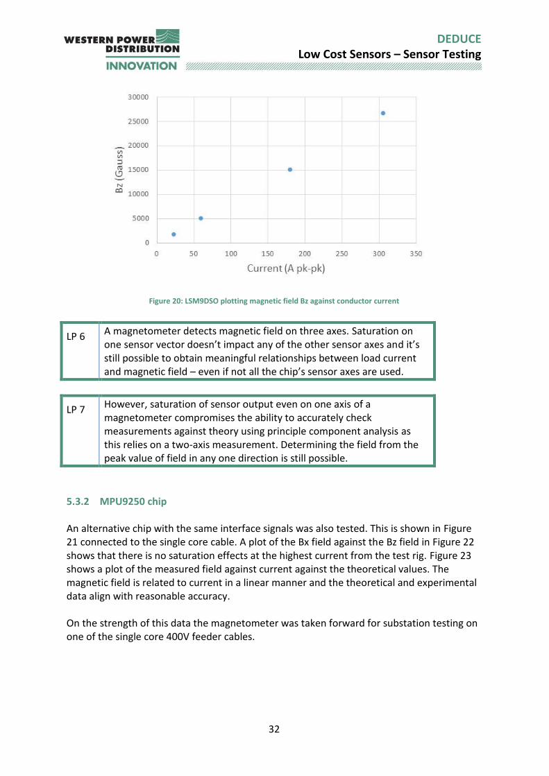
Figure 20: LSM9DSO plotting magnetic field Bz against conductor current
LP 6 A magnetometer detects magnetic field on three axes. Saturation on one sensor vector doesn’t impact any of the other sensor axes and it’s still possible to obtain meaningful relationships between load current and magnetic field – even if not all the chip’s sensor axes are used.
LP 7 However, saturation of sensor output even on one axis of a magnetometer compromises the ability to accurately check measurements against theory using principle component analysis as this relies on a two-axis measurement. Determining the field from the peak value of field in any one direction is still possible.
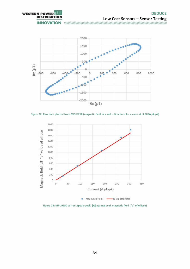
5.3.2 MPU9250 chip An alternative chip with the same interface signals was also tested. This is shown in Figure 21 connected to the single core cable. A plot of the Bx field against the Bz field in Figure 22 shows that there is no saturation effects at the highest current from the test rig. Figure 23 shows a plot of the measured field against current against the theoretical values. The magnetic field is related to current in a linear manner and the theoretical and experimental data align with reasonable accuracy. On the strength of this data the magnetometer was taken forward for substation testing on one of the single core 400V feeder cables.

33
DEDUCE Low Cost Sensors – Sensor Testing
Figure 21: Photo of MPU9250 magnetometer connected to the test rig
Magnetometer board
34
DEDUCE Low Cost Sensors – Sensor Testing
Figure 22: Raw data plotted from MPU9250 (magnetic field in x and z directions for a current of 308A pk-pk)
Figure 23: MPU9250 current (peak-peak) [A] against peak magnetic field (“a” of ellipse)
35
DEDUCE Low Cost Sensors – Sensor Testing
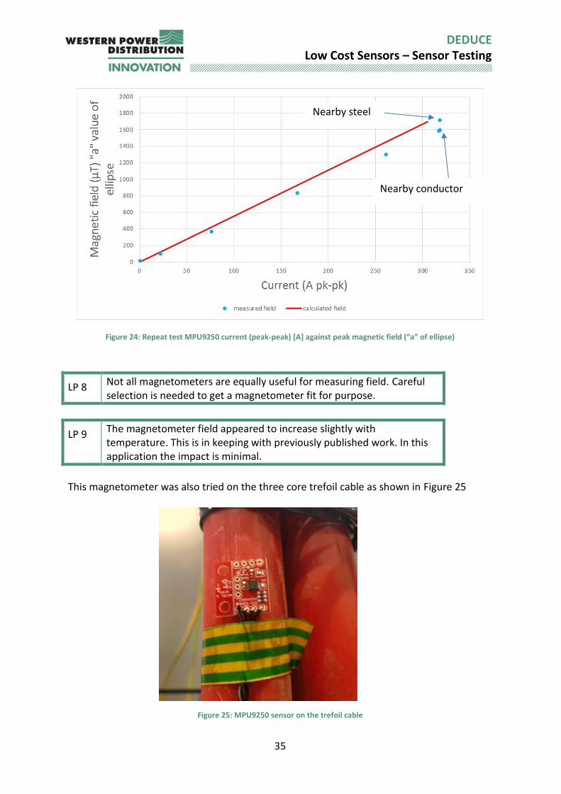
Figure 24: Repeat test MPU9250 current (peak-peak) [A] against peak magnetic field (“a” of ellipse)
LP 8 Not all magnetometers are equally useful for measuring field. Careful selection is needed to get a magnetometer fit for purpose.
LP 9 The magnetometer field appeared to increase slightly with temperature. This is in keeping with previously published work. In this application the impact is minimal.
This magnetometer was also tried on the three core trefoil cable as shown in Figure 25
Figure 25: MPU9250 sensor on the trefoil cable
Nearby steel
Nearby conductor
36
DEDUCE Low Cost Sensors – Sensor Testing
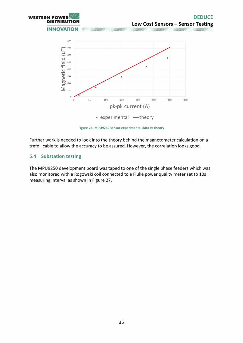
Figure 26: MPU9250 sensor experimental data vs theory
Further work is needed to look into the theory behind the magnetometer calculation on a trefoil cable to allow the accuracy to be assured. However, the correlation looks good.
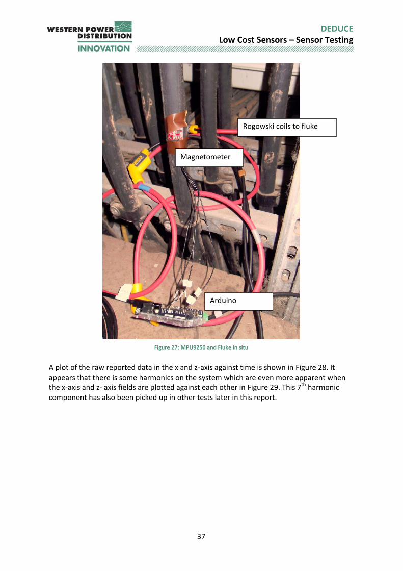
5.4 Substation testing The MPU9250 development board was taped to one of the single phase feeders which was also monitored with a Rogowski coil connected to a Fluke power quality meter set to 10s measuring interval as shown in Figure 27.
37
DEDUCE Low Cost Sensors – Sensor Testing
Figure 27: MPU9250 and Fluke in situ
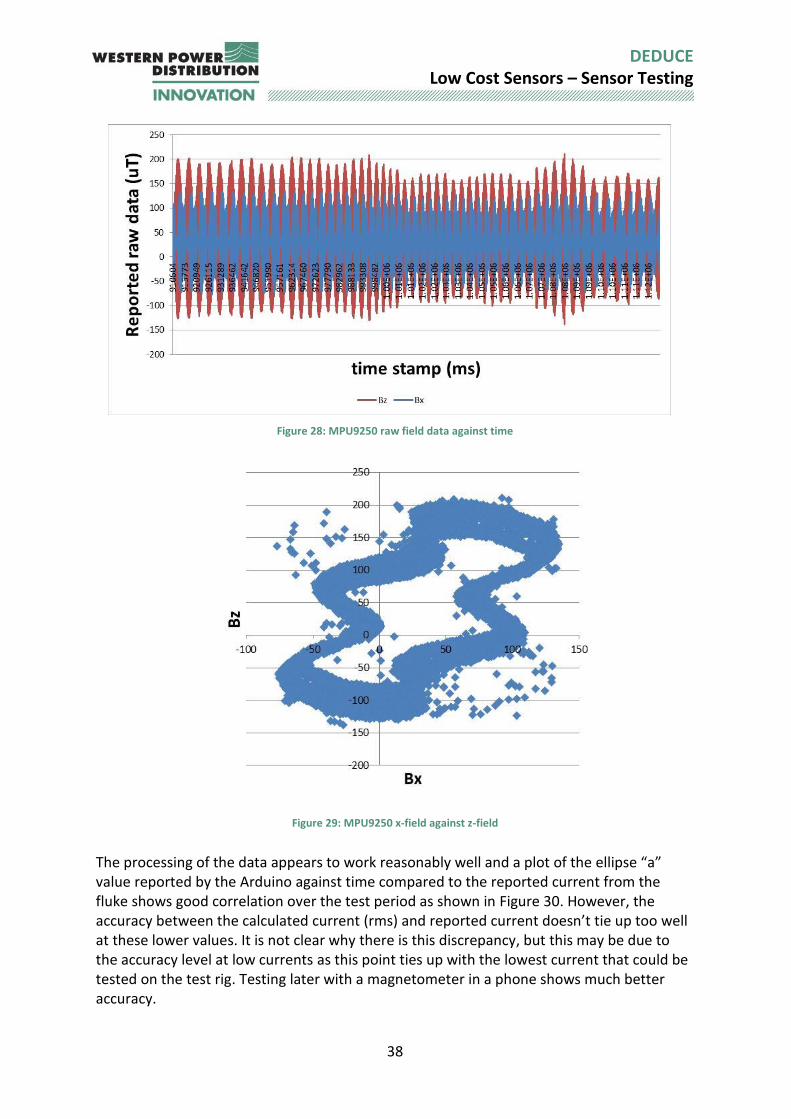
A plot of the raw reported data in the x and z-axis against time is shown in Figure 28. It appears that there is some harmonics on the system which are even more apparent when the x-axis and z- axis fields are plotted against each other in Figure 29. This 7th harmonic component has also been picked up in other tests later in this report.
Rogowski coils to fluke
Magnetometer
Arduino
38
DEDUCE Low Cost Sensors – Sensor Testing
Figure 28: MPU9250 raw field data against time
Figure 29: MPU9250 x-field against z-field
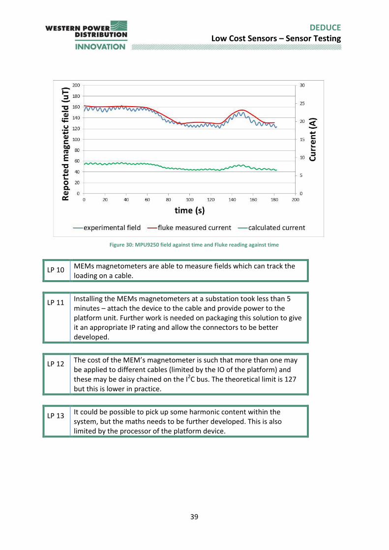
The processing of the data appears to work reasonably well and a plot of the ellipse “a” value reported by the Arduino against time compared to the reported current from the fluke shows good correlation over the test period as shown in Figure 30. However, the accuracy between the calculated current (rms) and reported current doesn’t tie up too well at these lower values. It is not clear why there is this discrepancy, but this may be due to the accuracy level at low currents as this point ties up with the lowest current that could be tested on the test rig. Testing later with a magnetometer in a phone shows much better accuracy.
39
DEDUCE Low Cost Sensors – Sensor Testing
Figure 30: MPU9250 field against time and Fluke reading against time
LP 10 MEMs magnetometers are able to measure fields which can track the loading on a cable.
LP 11 Installing the MEMs magnetometers at a substation took less than 5 minutes – attach the device to the cable and provide power to the platform unit. Further work is needed on packaging this solution to give it an appropriate IP rating and allow the connectors to be better developed.
LP 12 The cost of the MEM’s magnetometer is such that more than one may be applied to different cables (limited by the IO of the platform) and these may be daisy chained on the I2C bus. The theoretical limit is 127 but this is lower in practice.
LP 13 It could be possible to pick up some harmonic content within the system, but the maths needs to be further developed. This is also limited by the processor of the platform device.
40
DEDUCE Low Cost Sensors – Sensor Testing
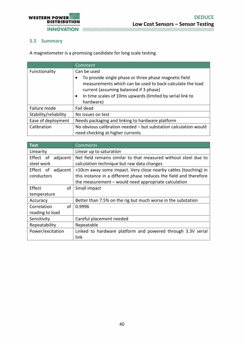
5.5 Summary A magnetometer is a promising candidate for long scale testing.
Comment
Functionality Can be used
To provide single phase or three phase magnetic field measurements which can be used to back-calculate the load current (assuming balanced if 3 phase)
In time scales of 10ms upwards (limited by serial link to hardware)
Failure mode Fail dead
Stability/reliability No issues on test
Ease of deployment Needs packaging and linking to hardware platform
Calibration No obvious calibration needed – but substation calculation would need checking at higher currents
Test Comments
Linearity Linear up to saturation
Effect of adjacent steel work
Net field remains similar to that measured without steel due to calculation technique but raw data changes
Effect of adjacent conductors
<10cm away some impact. Very close nearby cables (touching) in this instance in a different phase reduces the field and therefore the measurement – would need appropriate calculation
Effect of temperature
Small impact
Accuracy Better than 7.5% on the rig but much worse in the substation
Correlation of reading to load
0.9996
Sensitivity Careful placement needed
Repeatability Repeatable
Power/excitation Linked to hardware platform and powered through 3.3V serial link
41
DEDUCE Low Cost Sensors – Sensor Testing
6 Sensor B: Hall effect chip
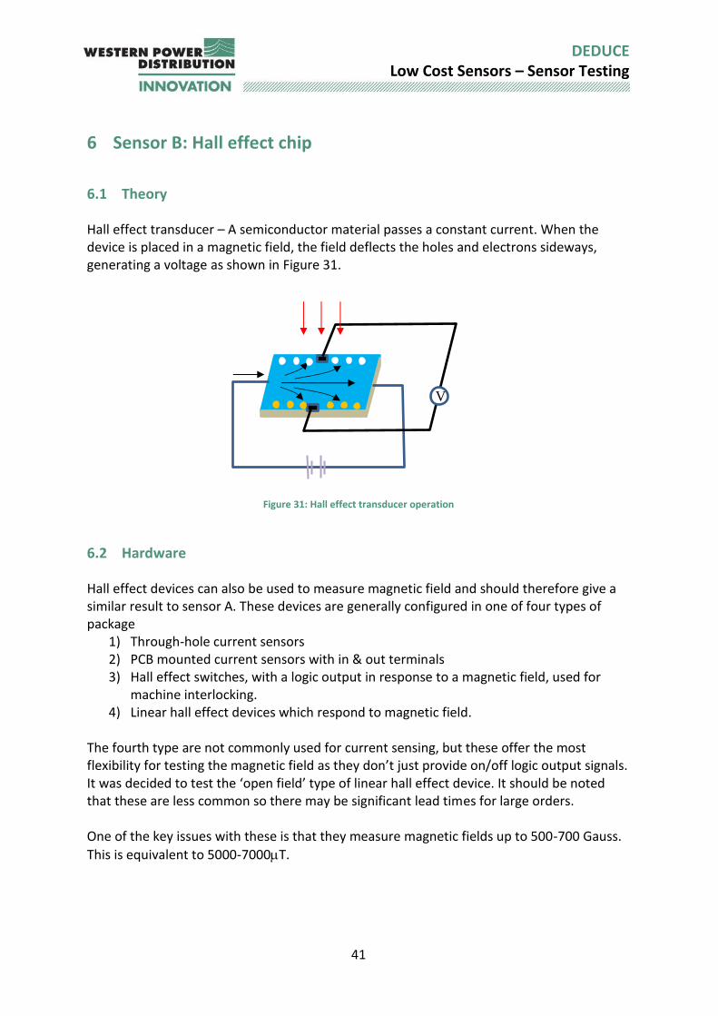
6.1 Theory Hall effect transducer – A semiconductor material passes a constant current. When the device is placed in a magnetic field, the field deflects the holes and electrons sideways, generating a voltage as shown in Figure 31.
Figure 31: Hall effect transducer operation
6.2 Hardware Hall effect devices can also be used to measure magnetic field and should therefore give a similar result to sensor A. These devices are generally configured in one of four types of package
1) Through-hole current sensors 2) PCB mounted current sensors with in & out terminals 3) Hall effect switches, with a logic output in response to a magnetic field, used for
machine interlocking. 4) Linear hall effect devices which respond to magnetic field.
The fourth type are not commonly used for current sensing, but these offer the most flexibility for testing the magnetic field as they don’t just provide on/off logic output signals. It was decided to test the ‘open field’ type of linear hall effect device. It should be noted that these are less common so there may be significant lead times for large orders. One of the key issues with these is that they measure magnetic fields up to 500-700 Gauss.
This is equivalent to 5000-7000T.
V

42
DEDUCE Low Cost Sensors – Sensor Testing
Table 6-1 : Cost of sensor B hardware
Vendor Part Qty Unit cost Line cost RS A1319LUA-5-T LHE chip 1 £1.75 £1.75
Farnell 0.1uF Capacitor 1 £0.14 £0.14 Farnell 10nF Capacitor 1 £0.12 £0.12 Farnell 47kR Resistor 1 £0.09 £0.09
Amazon Power supply 1 £4.99 £4.99
Rapid LinkitOne PCB (Arduino compatible) 1 £44.24 £44.24
System Total £51.33
The A1319LUA-5-T LHE chip looks like a transistor, has 3 legs and is supplied at 3- 3.6V. the device is stable with temperature and the claim is it provides an output voltage proportional to magnetic field. It is therefore suitable for connection with an Arduino board.
Figure 32: Photo of hall effect chip and its functional diagram
Figure 33: Photo of the linear hall effect device to the analogue input on an Arduino Uno
Vcc Vout
Gnd
43
DEDUCE Low Cost Sensors – Sensor Testing
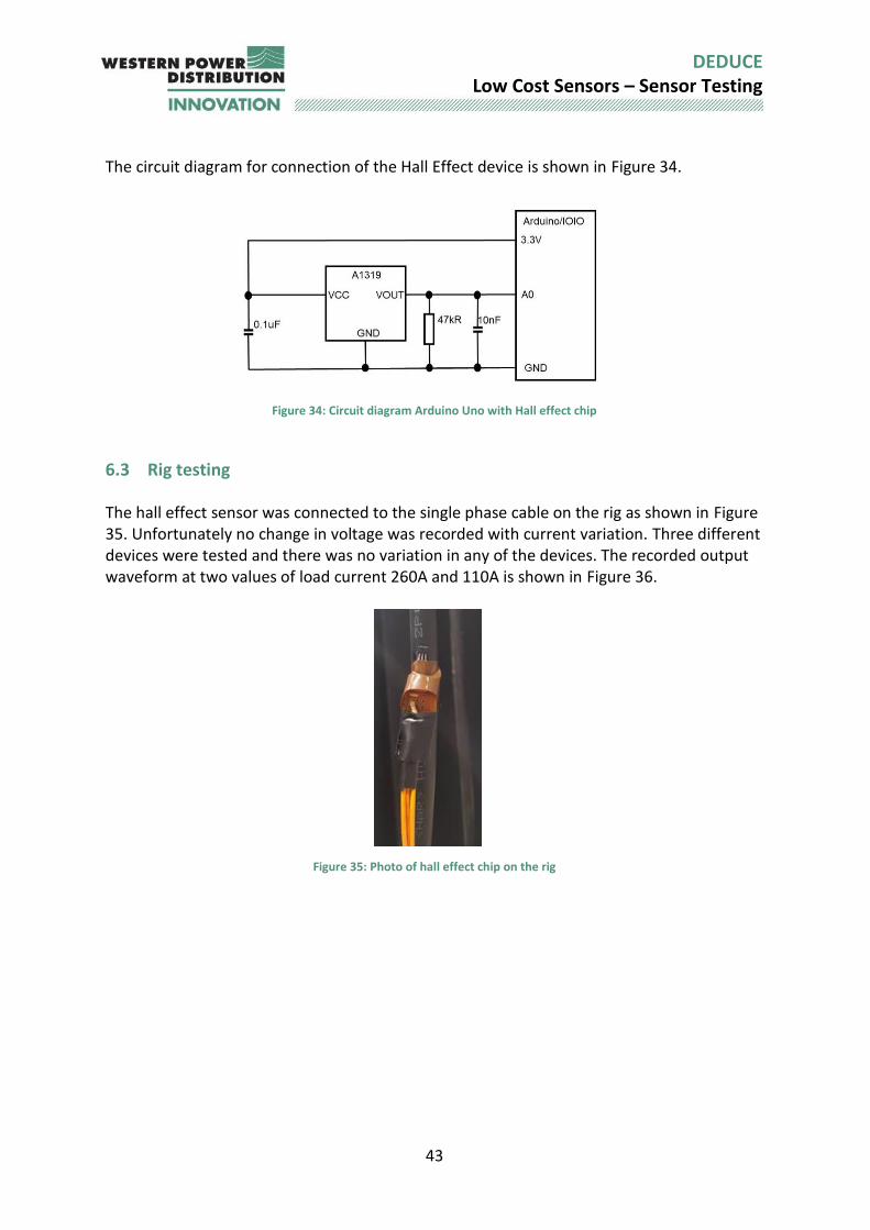
The circuit diagram for connection of the Hall Effect device is shown in Figure 34.
Figure 34: Circuit diagram Arduino Uno with Hall effect chip
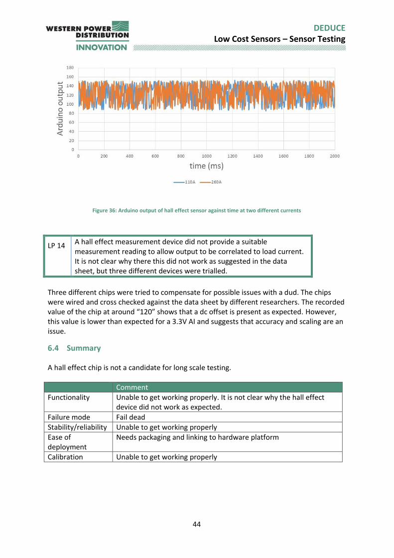
6.3 Rig testing The hall effect sensor was connected to the single phase cable on the rig as shown in Figure 35. Unfortunately no change in voltage was recorded with current variation. Three different devices were tested and there was no variation in any of the devices. The recorded output waveform at two values of load current 260A and 110A is shown in Figure 36.
Figure 35: Photo of hall effect chip on the rig
44
DEDUCE Low Cost Sensors – Sensor Testing
Figure 36: Arduino output of hall effect sensor against time at two different currents
LP 14 A hall effect measurement device did not provide a suitable measurement reading to allow output to be correlated to load current. It is not clear why there this did not work as suggested in the data sheet, but three different devices were trialled.
Three different chips were tried to compensate for possible issues with a dud. The chips were wired and cross checked against the data sheet by different researchers. The recorded value of the chip at around “120” shows that a dc offset is present as expected. However, this value is lower than expected for a 3.3V AI and suggests that accuracy and scaling are an issue.
6.4 Summary A hall effect chip is not a candidate for long scale testing.
Comment
Functionality Unable to get working properly. It is not clear why the hall effect device did not work as expected.
Failure mode Fail dead
Stability/reliability Unable to get working properly
Ease of deployment
Needs packaging and linking to hardware platform
Calibration Unable to get working properly
45
DEDUCE Low Cost Sensors – Sensor Testing
Test Comments
Linearity Unable to get working properly
Effect of adjacent steel work
Unable to get working properly
Effect of adjacent conductors
Unable to get working properly
Effect of temperature
Unable to get working properly
Accuracy Unable to get working properly
Correlation with load
Unable to get working properly
Sensitivity Unable to get working properly
Repeatability Unable to get working properly
Power/excitation Linked to hardware platform and powered through 3.3V serial link
46
DEDUCE Low Cost Sensors – Sensor Testing
7 Sensor C: i2m sensor
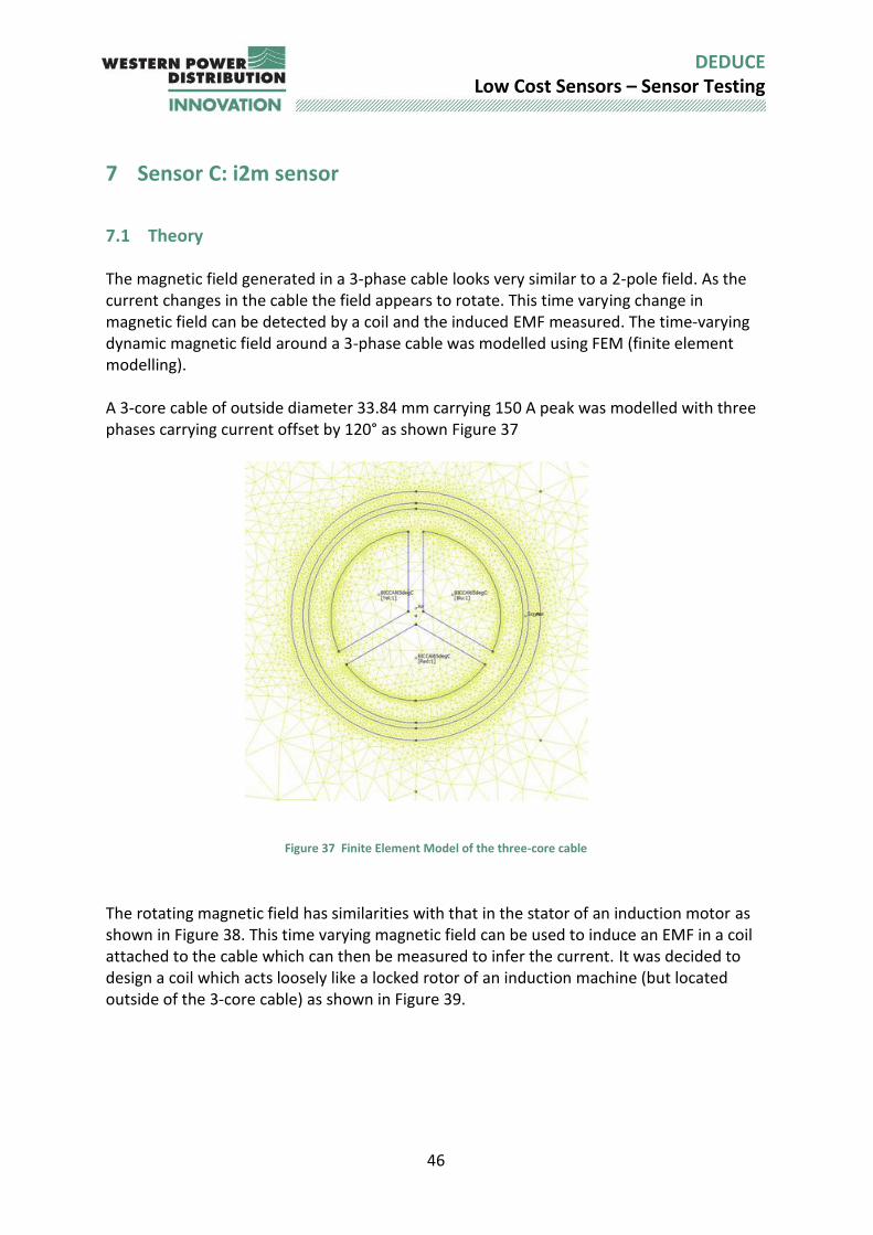
7.1 Theory The magnetic field generated in a 3-phase cable looks very similar to a 2-pole field. As the current changes in the cable the field appears to rotate. This time varying change in magnetic field can be detected by a coil and the induced EMF measured. The time-varying dynamic magnetic field around a 3-phase cable was modelled using FEM (finite element modelling). A 3-core cable of outside diameter 33.84 mm carrying 150 A peak was modelled with three phases carrying current offset by 120° as shown Figure 37
Figure 37 Finite Element Model of the three-core cable
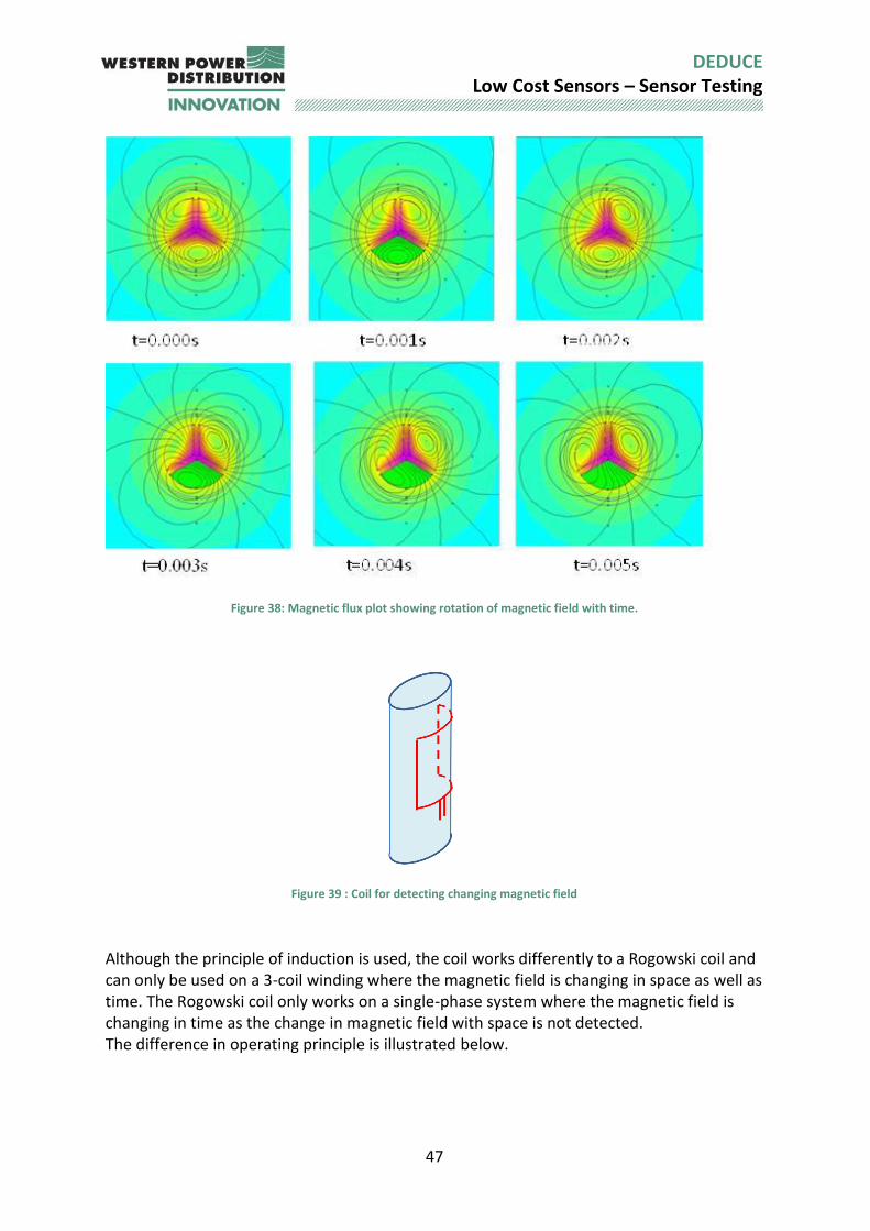
The rotating magnetic field has similarities with that in the stator of an induction motor as shown in Figure 38. This time varying magnetic field can be used to induce an EMF in a coil attached to the cable which can then be measured to infer the current. It was decided to design a coil which acts loosely like a locked rotor of an induction machine (but located outside of the 3-core cable) as shown in Figure 39.
47
DEDUCE Low Cost Sensors – Sensor Testing
Figure 38: Magnetic flux plot showing rotation of magnetic field with time.
Figure 39 : Coil for detecting changing magnetic field
Although the principle of induction is used, the coil works differently to a Rogowski coil and can only be used on a 3-coil winding where the magnetic field is changing in space as well as time. The Rogowski coil only works on a single-phase system where the magnetic field is changing in time as the change in magnetic field with space is not detected. The difference in operating principle is illustrated below.
48
DEDUCE Low Cost Sensors – Sensor Testing
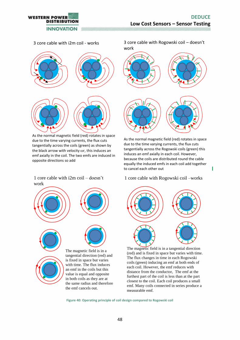
Figure 40: Operating principle of coil design compared to Rogowski coil
3 core cable with i2m coil - works
As the normal magnetic field (red) rotates in space due to the time varying currents, the flux cuts tangentially across the coils (green) as shown by
the black arrow with velocity r, this induces an emf axially in the coil. The two emfs are induced in opposite directions so add
3 core cable with Rogowski coil – doesn’t work
As the normal magnetic field (red) rotates in space due to the time varying currents, the flux cuts tangentially across the Rogowski coils (green) this induces an emf axially in each coil. However, because the coils are distributed round the cable equally the induced emfs in each coil add together to cancel each other out
1 core cable with i2m coil – doesn’t
work
The magnetic field is in a
tangential direction (red) and
is fixed in space but varies
with time. The flux induces
an emf in the coils but this
value is equal and opposite
in both coils as they are at
the same radius and therefore
the emf cancels out.
1 core cable with Rogowski coil –works
The magnetic field is in a tangential direction
(red) and is fixed in space but varies with time.
The flux changes in time in each Rogowski
coils (green) inducing an emf at both ends of
each coil. However, the emf reduces with
distance from the conductor, The emf at the
furthest part of the coil is less than at the part
closest to the coil. Each coil produces a small
emf. Many coils connected in series produce a
measurable emf.
49
DEDUCE Low Cost Sensors – Sensor Testing
The induced EMF in the i2m coil with around a 3-core cable (or 3 single cores in a trefoil arrangement) can be estimated using Faraday’s Law directly (Equation 7-1) or through derivations from the integral form of the Maxwell-Faraday equation. Both yield the same answer, however itis useful to derive from first principles to aid understanding. Deriving through Faraday’s equation; 𝑒 is the induced voltage [volts], N is the number of turns in the coil and 𝜑 is the flux [Wb].
𝑒 = −𝑁𝑑𝜑
𝑑𝑡 Equation 7-1
If it is assumed that the flux density, B is changing sinusoidally around the conductor as per (Equation 7-2), then the induced EMF in the coil can be calculated from (Equation 7-3)
𝐵 = ��𝑠𝑖𝑛(𝜔𝑡 + 𝜃) Equation 7-2
Where 𝜔 = 2𝜋𝑓 (rad).
𝑒 = −2𝑁𝜔𝑟𝑙��𝑐𝑜𝑠(𝜔𝑡 + 𝜃) Equation 7-3
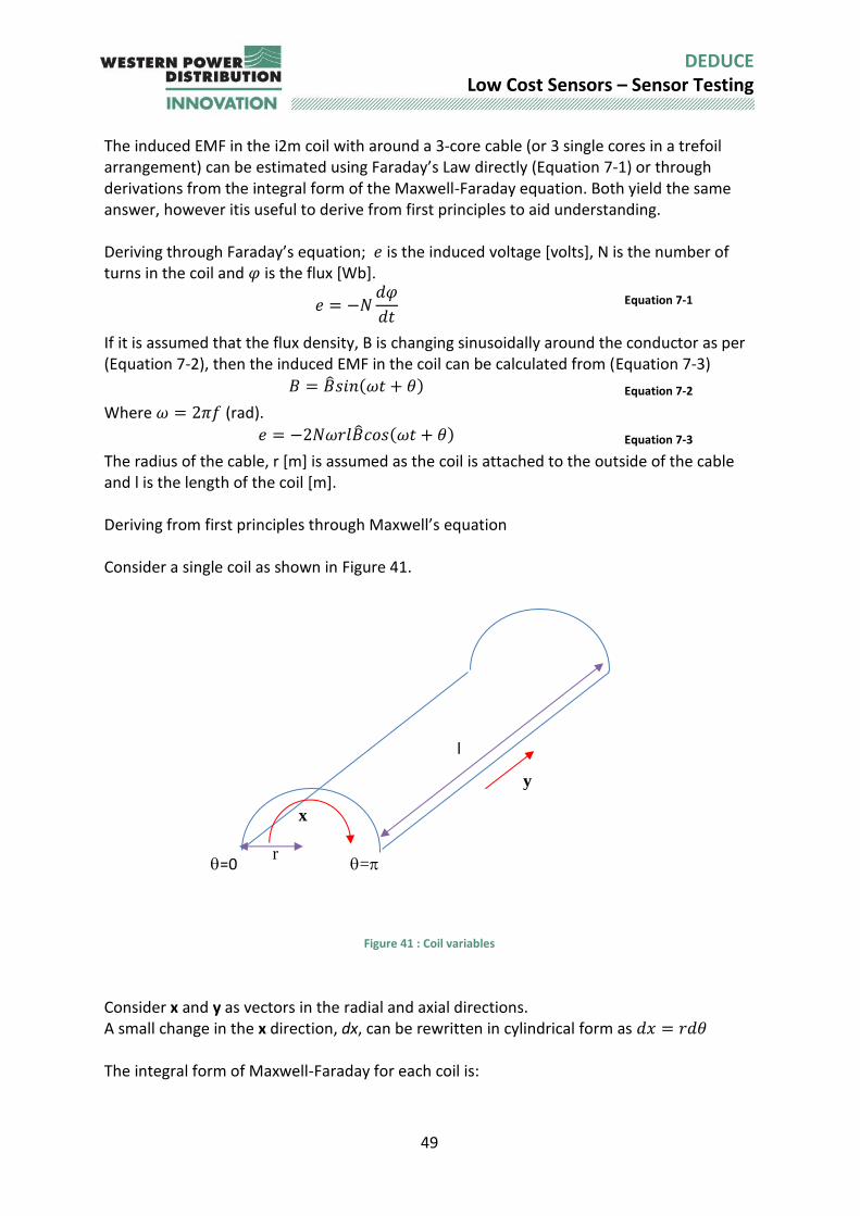
The radius of the cable, r [m] is assumed as the coil is attached to the outside of the cable and l is the length of the coil [m]. Deriving from first principles through Maxwell’s equation Consider a single coil as shown in Figure 41.
Figure 41 : Coil variables
Consider x and y as vectors in the radial and axial directions. A small change in the x direction, dx, can be rewritten in cylindrical form as 𝑑𝑥 = 𝑟𝑑𝜃 The integral form of Maxwell-Faraday for each coil is:
=0 =
x
y
r
l
50
DEDUCE Low Cost Sensors – Sensor Testing
𝑉 = ∮ 𝐸 ∙ 𝑑𝑙 = −𝑑
𝑑𝑡∬ 𝐵 ∙ 𝑑𝑆
𝑆
Equation 7-4
Substituting for B from Equation 7-2
𝑉 = −𝑑
𝑑𝑡∫ ∫ ��𝑠𝑖𝑛(𝜔𝑡 + 𝜃) 𝑑𝑦 𝑑𝑥
𝑦=𝑙
𝑦=0
𝑥=𝑟𝜃
𝑥=0
Equation 7-5
Substituting for dx
𝑉 = −𝑑
𝑑𝑡∫ ∫ 𝑟��𝑠𝑖𝑛(𝜔𝑡 + 𝜃) 𝑑𝑦 𝑑𝜃
𝑦=𝑙
𝑦=0
𝜃=𝜋
𝜃=0
Equation 7-6
Integrating gives
𝑉 = −𝑑
𝑑𝑡(−2𝑟𝑙��𝑐𝑜𝑠(𝜔𝑡)) Equation 7-7
Then taking the time differential gives
𝑉 = −𝑑
𝑑𝑡(−2𝑟𝑙��𝑐𝑜𝑠(𝜔𝑡)) Equation 7-8
𝑉 = −2𝜔𝑟𝑙��𝑠𝑖𝑛(𝜔𝑡) Equation 7-9
This is the same as Equation 7-3, where = and the number of turns of coil =N. To achieve a sufficiently high induced EMF and an acceptable signal to noise ratio (SNR), the coils were designed to be 200 mm long and have 15 turns. As the magnetic field from the 3 coils rotates like a 2-pole machine, the coil is designed to go 180° around the cable as shown. Having additional coils offset by 120° allows the rotating field to be observed in each of the coils. While it is desirable to have this information (and it could give indication of unbalance and current direction if a reference voltage is present) this is not essential. Using these values in Equation 7-3 with a peak magnetic field (from the FEM) gives an induced EMF in each coil of approximately 60 mV. The output from the coils can then sent to an isolating level shift and amplifier circuit before being connected through to a GPRS Arduino platform for sending the readings to a server.
The main purpose of detecting the voltage is to derive the current in the cable. As this research is in preliminary stages, it is assumed, in this case, that the currents in the cable are balanced. Under this scenario, an estimate of current can be made by assuming the current as a point source at the center of each sector and using the geometrical parameters in Figure 42 with reference to and using the following equations to back calculate the

51
DEDUCE Low Cost Sensors – Sensor Testing
current. Using multiple coils located around the outside of the cable could allow unbalanced currents to be calculated. However, the mathematics in determining this is involved and outside of the scope of the current project.
Figure 42: Simplified model of 3 core sectored cable and location of coil
The distance from the center of a sector to its centroid is found from Equation 7-10.
𝑑 =2𝑟3sin (𝛼)
3𝛼 Equation 7-10
Where is the half angle of the sector (60o). While the distance from the center of conductor Y to one end of the coil is found from Equation 7-11 and a similar expression can be found between the center of Y and the other side of the coil:
𝑟4 = √𝑟22 + (𝑟1 + 𝑑)2 − 2𝑟2(𝑟1 + 𝑑)𝑐𝑜𝑠(120𝑜) Equation 7-11
It is necessary to calculate the normal component of flux density at each end of the coil due to the currents in each of the three phases. As this has been aligned specifically with the R phase so normal component exists, the maths may be simplified. An example of the normal field in the bottom part of the coil due to the current in Y, is shown by the green arrow in Fig. 5 and can be calculated from Equation 7-12.
𝐵𝑛 =𝜇𝑜𝐼𝑌
2𝜋𝑟4.(𝑟1 + 𝑑)
𝑟4sin (120𝑜) Equation 7-12
With balanced currents, the peak emf can be found from the magnetic field through Equation 7-9 and Equation 7-12 as
Y d
r2
r1
R
B
e+
e-
r4
r5
r3
52
DEDUCE Low Cost Sensors – Sensor Testing
�� = 3𝑁𝑟22𝑙𝑓
𝜇𝑜𝐼
2(
1
𝑟42
+1
𝑟52
) Equation 7-13
Rearranging gives an estimate of peak current in each phase as
𝐼 =��
3𝑁𝑓(𝑑 + 𝑟1)𝑟2𝑙𝜇𝑜 (1
𝑟42 +
1𝑟5
2) Equation 7-14
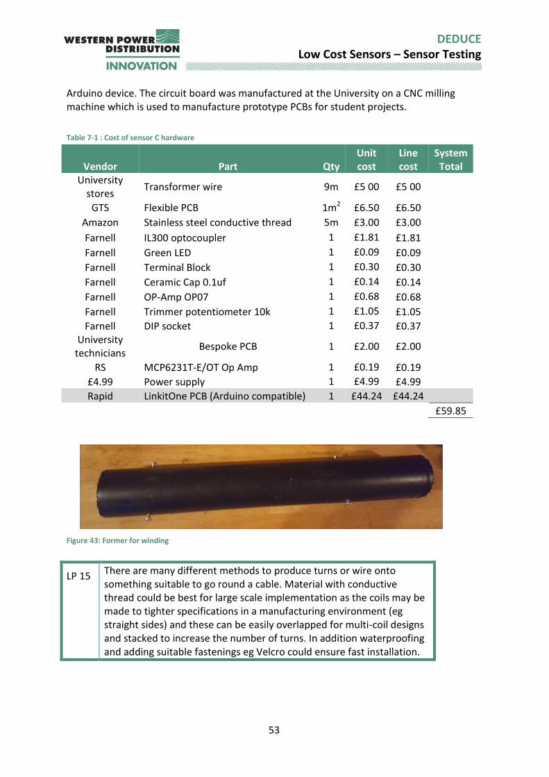
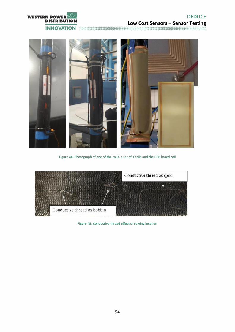
7.2 Hardware There are a number of methods of producing a suitable coil. For example, the coil can be made traditionally using insulated wire. As the coils are positioned in air rather than laminated steel (which would be too expensive and complex) the induced voltage in the coils is around 60 mV per 100 A of primary cable current. The coil can be wound round a former as shown in Figure 43 and then taped together before being fixed to the cable with cable ties linking each corner. This is a low cost and effective means of installation. The coil must be sufficiently rigid to install in this means which is why the thinnest transformer wire was not used. The coils are manufactured on a former from varnish insulated ‘enamel’ copper transformer wire (0.5 mm diameter). There is an additional design trade-off between the number of turns and the length of the coil. Coiling hundreds of turns similar to a Rogowski coil is time consuming and impacts the radius that the coil is located at. The coil is shown in Figure 44. A coil design is not an exact solution, so an alternative design was also manufactured using copper printing on flexible PCB material. It was more straightforward to get exact coils in a suitable location, but the width of the tracks was fine in places and the track broke when the tracks were too fine. Several tries were needed to arrive at 1mm track width. It was difficult to solder the connections to the coil and great care was needed to provide support for the connection wires so these could not be pulled loose. This makes it unsuitable in its present form for a rugged substation environment. The alternative PCB based design had copper tracks of 1 mm and was 16 turns with 8 turns printed on each side and a common connector as shown in Figure 44. A third alternative is to use conductive thread on material. Two types of thread were trialled steel covered nylon and silver coated copper. The former is easier to sew with while the latter is easier to solder onto. Figure 45 shows early attempts at machine sewing the conductive thread. Tension is an issue and therefore it is recommended the thread is sewn as the bobbin rather than the spool. Even once the tension is sorted, it is necessary to keep an eye on the sewing as loops which can be caught by other wires are all to easy to create as shown in Figure 46. This isn’t an issue with hand sewn – but this was add cost and is not as exact a solution and less turns will be present in the available space. It is necessary to amplify the coil output to achieve a voltage above the noise floor of the controller board. A bespoke signal amplifier circuit based on an MCP6231 op-amp is used to amplify the voltage signal from the sensor for compatibility with analogue inputs on an
53
DEDUCE Low Cost Sensors – Sensor Testing
Arduino device. The circuit board was manufactured at the University on a CNC milling machine which is used to manufacture prototype PCBs for student projects.
Table 7-1 : Cost of sensor C hardware
Vendor Part Qty Unit cost
Line cost
System Total
University stores
Transformer wire 9m £5 00 £5 00
GTS Flexible PCB 1m2 £6.50 £6.50
Amazon Stainless steel conductive thread 5m £3.00 £3.00
Farnell IL300 optocoupler 1 £1.81 £1.81 Farnell Green LED 1 £0.09 £0.09 Farnell Terminal Block 1 £0.30 £0.30 Farnell Ceramic Cap 0.1uf 1 £0.14 £0.14 Farnell OP-Amp OP07 1 £0.68 £0.68 Farnell Trimmer potentiometer 10k 1 £1.05 £1.05 Farnell DIP socket 1 £0.37 £0.37 University
technicians Bespoke PCB 1 £2.00 £2.00
RS MCP6231T-E/OT Op Amp 1 £0.19 £0.19 £4.99 Power supply 1 £4.99 £4.99
Rapid LinkitOne PCB (Arduino compatible) 1 £44.24 £44.24
£59.85
Figure 43: Former for winding
LP 15 There are many different methods to produce turns or wire onto something suitable to go round a cable. Material with conductive thread could be best for large scale implementation as the coils may be made to tighter specifications in a manufacturing environment (eg straight sides) and these can be easily overlapped for multi-coil designs and stacked to increase the number of turns. In addition waterproofing and adding suitable fastenings eg Velcro could ensure fast installation.
54
DEDUCE Low Cost Sensors – Sensor Testing
Figure 44: Photograph of one of the coils, a set of 3 coils and the PCB based coil
Figure 45: Conductive thread effect of sewing location
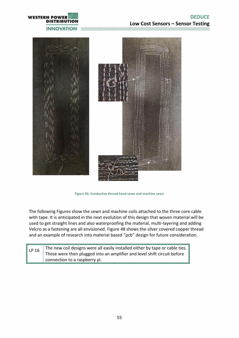
55
DEDUCE Low Cost Sensors – Sensor Testing
Figure 46: Conductive thread hand sewn and machine sewn
The following Figures show the sewn and machine coils attached to the three core cable with tape. It is anticipated in the next evolution of this design that woven material will be used to get straight lines and also waterproofing the material, multi-layering and adding Velcro as a fastening are all envisioned. Figure 48 shows the silver covered copper thread and an example of research into material based “pcb” design for future consideration.
LP 16 The new coil designs were all easily installed either by tape or cable ties. These were then plugged into an amplifier and level shift circuit before connection to a raspberry pi.

56
DEDUCE Low Cost Sensors – Sensor Testing
Figure 47: Conductive thread mounted on cable (hand sewn and machine sewn)
Figure 48: Solderable thread and an example of material based “pcb” design
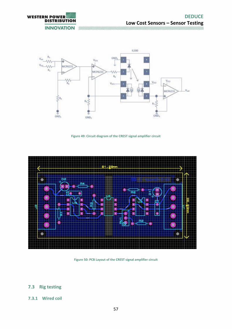
57
DEDUCE Low Cost Sensors – Sensor Testing
Figure 49: Circuit diagram of the CREST signal amplifier circuit
Figure 50: PCB Layout of the CREST signal amplifier circuit
7.3 Rig testing 7.3.1 Wired coil
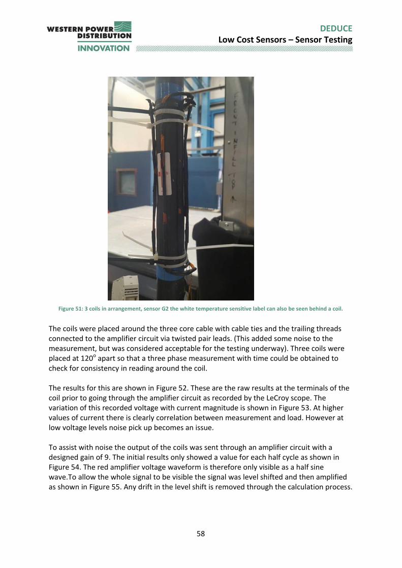
58
DEDUCE Low Cost Sensors – Sensor Testing
Figure 51: 3 coils in arrangement, sensor G2 the white temperature sensitive label can also be seen behind a coil.
The coils were placed around the three core cable with cable ties and the trailing threads connected to the amplifier circuit via twisted pair leads. (This added some noise to the measurement, but was considered acceptable for the testing underway). Three coils were placed at 120o apart so that a three phase measurement with time could be obtained to check for consistency in reading around the coil. The results for this are shown in Figure 52. These are the raw results at the terminals of the coil prior to going through the amplifier circuit as recorded by the LeCroy scope. The variation of this recorded voltage with current magnitude is shown in Figure 53. At higher values of current there is clearly correlation between measurement and load. However at low voltage levels noise pick up becomes an issue. To assist with noise the output of the coils was sent through an amplifier circuit with a designed gain of 9. The initial results only showed a value for each half cycle as shown in Figure 54. The red amplifier voltage waveform is therefore only visible as a half sine wave.To allow the whole signal to be visible the signal was level shifted and then amplified as shown in Figure 55. Any drift in the level shift is removed through the calculation process.
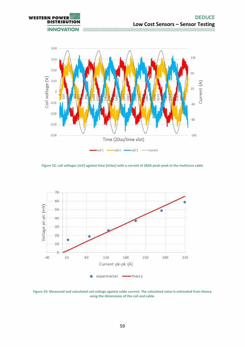
59
DEDUCE Low Cost Sensors – Sensor Testing
Figure 52: coil voltages [mV] against time [mSec] with a current of 260A peak-peak in the multicore cable
Figure 53: Measured and calculated coil voltage against cable current. The calculated value is estimated from theory using the dimensions of the coil and cable.
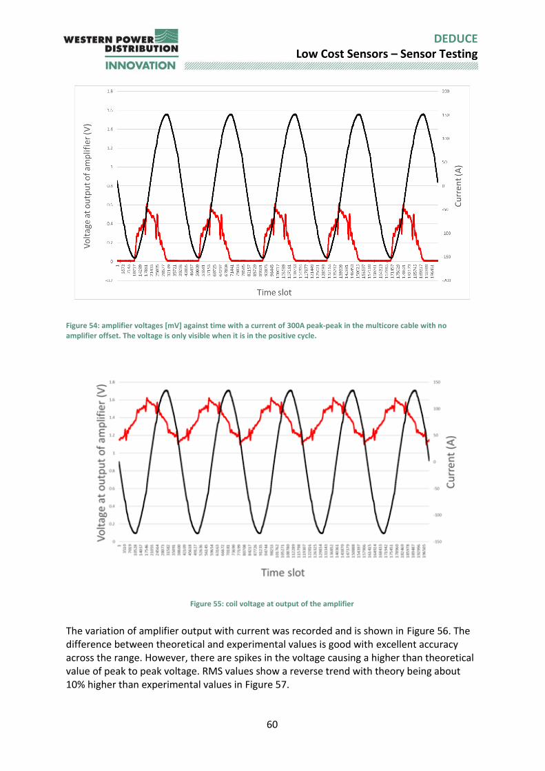
60
DEDUCE Low Cost Sensors – Sensor Testing
Figure 54: amplifier voltages [mV] against time with a current of 300A peak-peak in the multicore cable with no amplifier offset. The voltage is only visible when it is in the positive cycle.
Figure 55: coil voltage at output of the amplifier
The variation of amplifier output with current was recorded and is shown in Figure 56. The difference between theoretical and experimental values is good with excellent accuracy across the range. However, there are spikes in the voltage causing a higher than theoretical value of peak to peak voltage. RMS values show a reverse trend with theory being about 10% higher than experimental values in Figure 57.
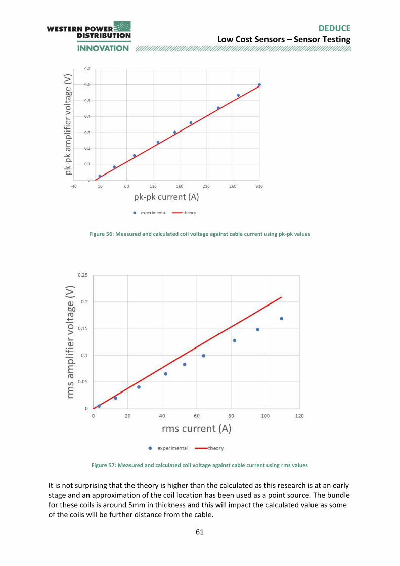
61
DEDUCE Low Cost Sensors – Sensor Testing
Figure 56: Measured and calculated coil voltage against cable current using pk-pk values
Figure 57: Measured and calculated coil voltage against cable current using rms values
It is not surprising that the theory is higher than the calculated as this research is at an early stage and an approximation of the coil location has been used as a point source. The bundle for these coils is around 5mm in thickness and this will impact the calculated value as some of the coils will be further distance from the cable.
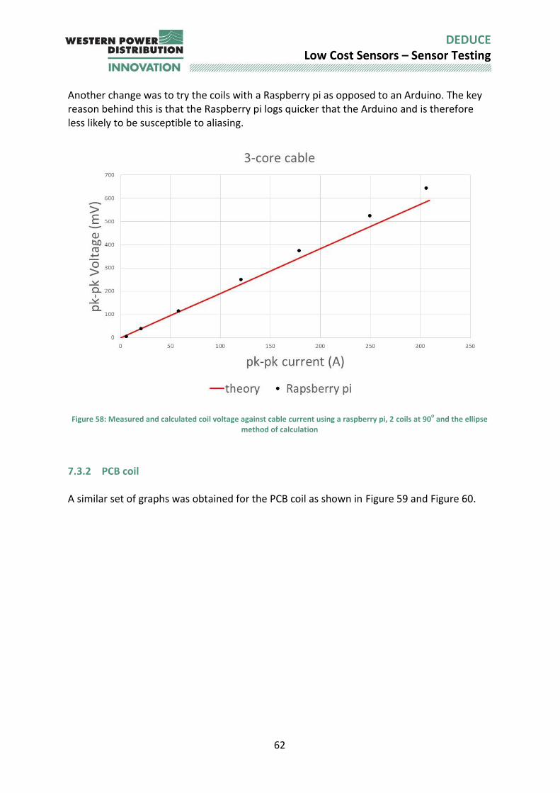
62
DEDUCE Low Cost Sensors – Sensor Testing
Another change was to try the coils with a Raspberry pi as opposed to an Arduino. The key reason behind this is that the Raspberry pi logs quicker that the Arduino and is therefore less likely to be susceptible to aliasing.
Figure 58: Measured and calculated coil voltage against cable current using a raspberry pi, 2 coils at 90
o and the ellipse
method of calculation
7.3.2 PCB coil A similar set of graphs was obtained for the PCB coil as shown in Figure 59 and Figure 60.
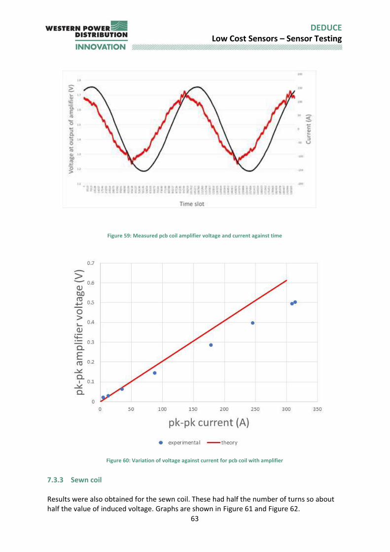
63
DEDUCE Low Cost Sensors – Sensor Testing
Figure 59: Measured pcb coil amplifier voltage and current against time
Figure 60: Variation of voltage against current for pcb coil with amplifier
7.3.3 Sewn coil Results were also obtained for the sewn coil. These had half the number of turns so about half the value of induced voltage. Graphs are shown in Figure 61 and Figure 62.
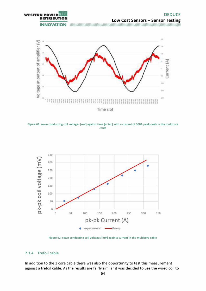
64
DEDUCE Low Cost Sensors – Sensor Testing
Figure 61: sewn conducting coil voltages [mV] against time [mSec] with a current of 300A peak-peak in the multicore cable
Figure 62: sewn conducting coil voltages [mV] against current in the multicore cable
7.3.4 Trefoil cable In addition to the 3 core cable there was also the opportunity to test this measurement against a trefoil cable. As the results are fairly similar it was decided to use the wired coil to
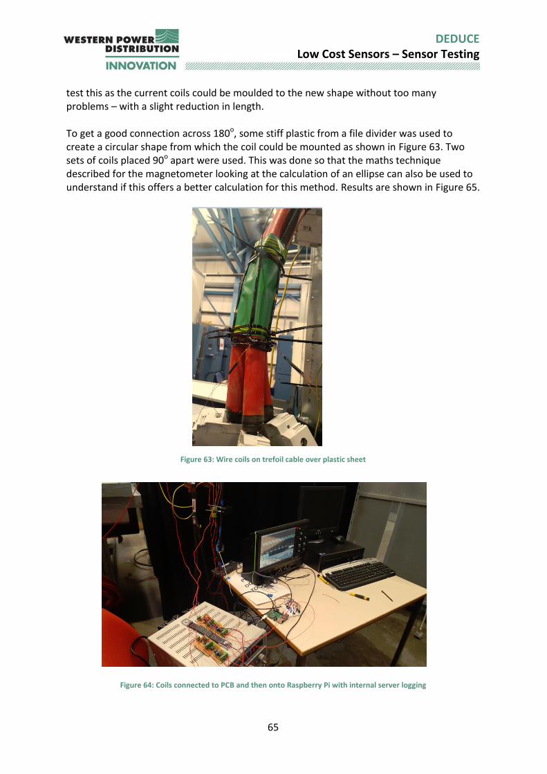
65
DEDUCE Low Cost Sensors – Sensor Testing
test this as the current coils could be moulded to the new shape without too many problems – with a slight reduction in length. To get a good connection across 180o, some stiff plastic from a file divider was used to create a circular shape from which the coil could be mounted as shown in Figure 63. Two sets of coils placed 90o apart were used. This was done so that the maths technique described for the magnetometer looking at the calculation of an ellipse can also be used to understand if this offers a better calculation for this method. Results are shown in Figure 65.
Figure 63: Wire coils on trefoil cable over plastic sheet
Figure 64: Coils connected to PCB and then onto Raspberry Pi with internal server logging

66
DEDUCE Low Cost Sensors – Sensor Testing
Figure 65: experimental and theoretical results of two coils at 90
o with field calculated through ellipse theory.
7.3.5 Comparison of all types Each of the three coils gave a good degree of correlation between load current and measured voltage signal as shown in Table 7-2. The comparison with theory showed around a 10% underestimate of load current based on measurement. However, it is fairly clear that this is due to two factors;
1. The bundling of the wire coil which results in distances changing between coils of wire.
2. The PCB and sewn coil have distributed windings and this will act to lower the field in the bundled set. Resulting in an underestimate.
Further work is needed to go through the maths and modify the back calculation to adjust for these.
Table 7-2 : correlation of sensor measurement and theory with current
Coil Correlation co-efficient
Wound coil 0.999
PCB 0.999
Sewn coil 0.996

67
DEDUCE Low Cost Sensors – Sensor Testing
LP 17 The new coil designs showed good correlation between measurement and load current in a balanced system.
LP 18 At this stage the maths behind the i2m coil needs further development to take into account factors such as the distributed nature of the windings or the lumping together of the windings and also to look at imbalance.
LP 19 There was no impact on the readings in the presence of a thermal source (heat gun) and only a very small change in value with close by metal work.
7.4 Substation testing The three coils were installed on the 11kV cable between the RMU and the transformer. Installation can be seen in Figure 66. The results were firstly captured on the LeCroy scope and then on the Arduino through the analogue input channels A0, A1 and A2. The sewn and PCB coils were directly above each other and the vertical axis was carefully aligned. This meant that the captured data could be more easily compared as shown in Figure 67. There isn’t a large variation in value but these are clearly changing at the same time. The sewn coil is very noisy because it was connected up on site and it was difficult to get a good connection on one of the wires. Pre-installation of the coil to cable is necessary to avoid this issue. The coils are then connected to the amplifier before being connected to the scope. A close up on the AC coupled waveforms of the three coils is shown in Figure 68 and Figure 69. The sewn thread output has been multiplied by a factor of 2 to show the similarity against the PCB value. This latter curve also clearly shows a 7th harmonic ripple on the current measurement value.
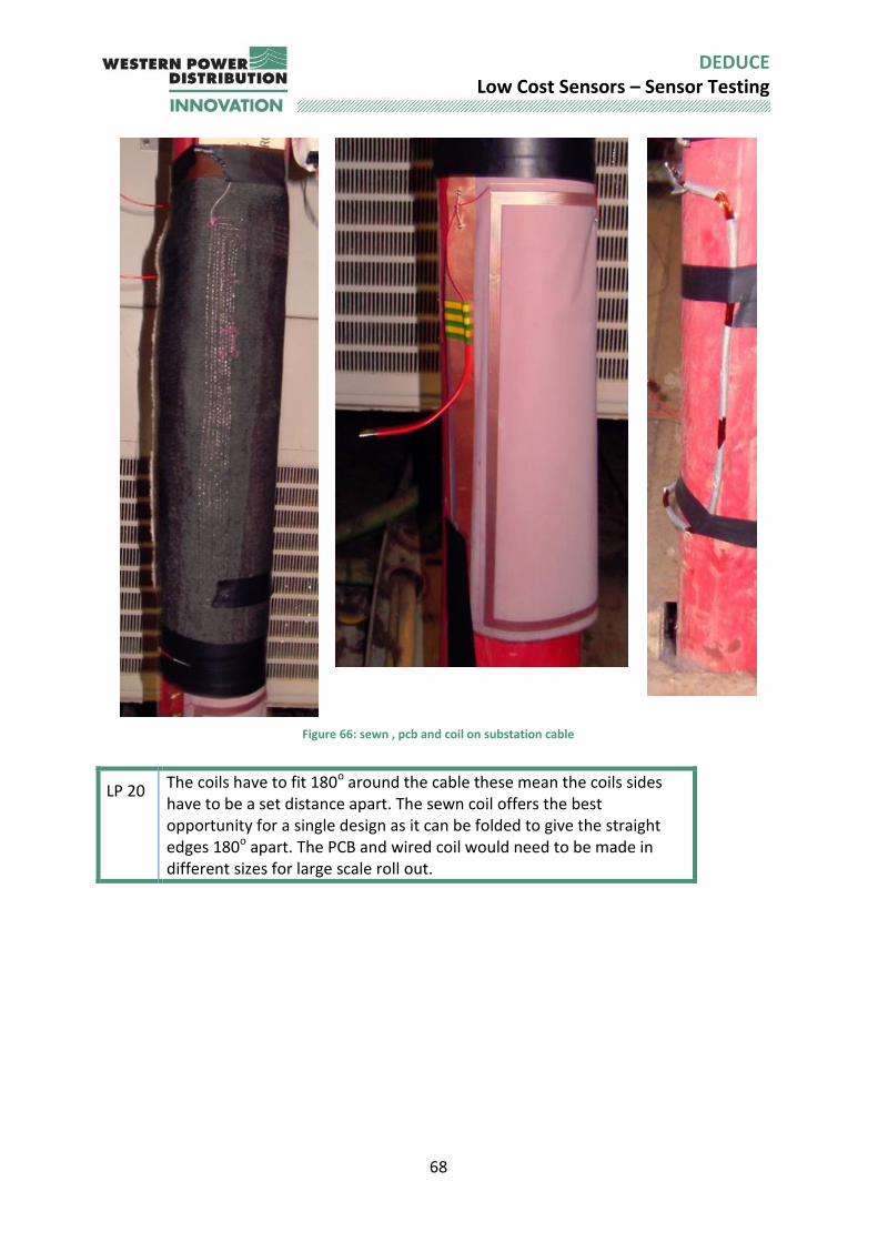
68
DEDUCE Low Cost Sensors – Sensor Testing
Figure 66: sewn , pcb and coil on substation cable
LP 20 The coils have to fit 180o around the cable these mean the coils sides have to be a set distance apart. The sewn coil offers the best opportunity for a single design as it can be folded to give the straight edges 180o apart. The PCB and wired coil would need to be made in different sizes for large scale roll out.
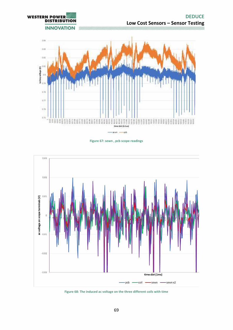
69
DEDUCE Low Cost Sensors – Sensor Testing
Figure 67: sewn , pcb scope readings
Figure 68: The induced ac voltage on the three different coils with time
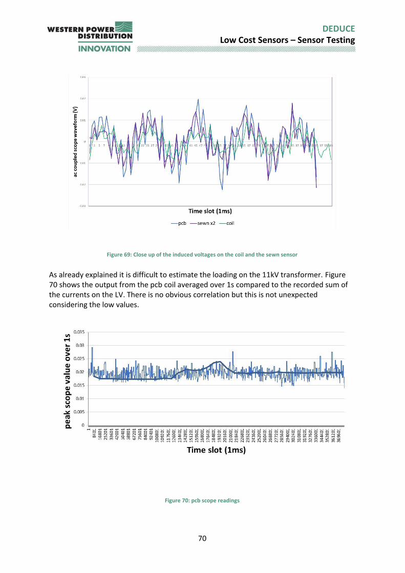
70
DEDUCE Low Cost Sensors – Sensor Testing
Figure 69: Close up of the induced voltages on the coil and the sewn sensor
As already explained it is difficult to estimate the loading on the 11kV transformer. Figure 70 shows the output from the pcb coil averaged over 1s compared to the recorded sum of the currents on the LV. There is no obvious correlation but this is not unexpected considering the low values.
Figure 70: pcb scope readings
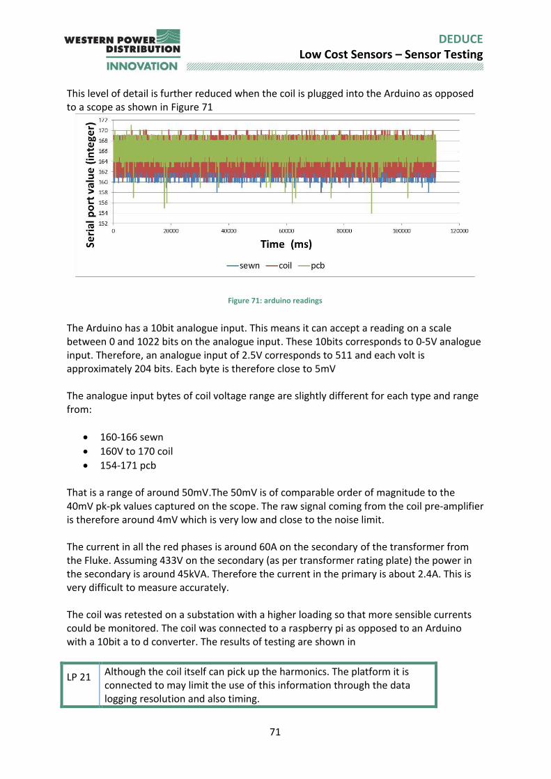
71
DEDUCE Low Cost Sensors – Sensor Testing
This level of detail is further reduced when the coil is plugged into the Arduino as opposed to a scope as shown in Figure 71
Figure 71: arduino readings
The Arduino has a 10bit analogue input. This means it can accept a reading on a scale between 0 and 1022 bits on the analogue input. These 10bits corresponds to 0-5V analogue input. Therefore, an analogue input of 2.5V corresponds to 511 and each volt is approximately 204 bits. Each byte is therefore close to 5mV The analogue input bytes of coil voltage range are slightly different for each type and range from:
160-166 sewn
160V to 170 coil
154-171 pcb That is a range of around 50mV.The 50mV is of comparable order of magnitude to the 40mV pk-pk values captured on the scope. The raw signal coming from the coil pre-amplifier is therefore around 4mV which is very low and close to the noise limit. The current in all the red phases is around 60A on the secondary of the transformer from the Fluke. Assuming 433V on the secondary (as per transformer rating plate) the power in the secondary is around 45kVA. Therefore the current in the primary is about 2.4A. This is very difficult to measure accurately. The coil was retested on a substation with a higher loading so that more sensible currents could be monitored. The coil was connected to a raspberry pi as opposed to an Arduino with a 10bit a to d converter. The results of testing are shown in
LP 21 Although the coil itself can pick up the harmonics. The platform it is connected to may limit the use of this information through the data logging resolution and also timing.
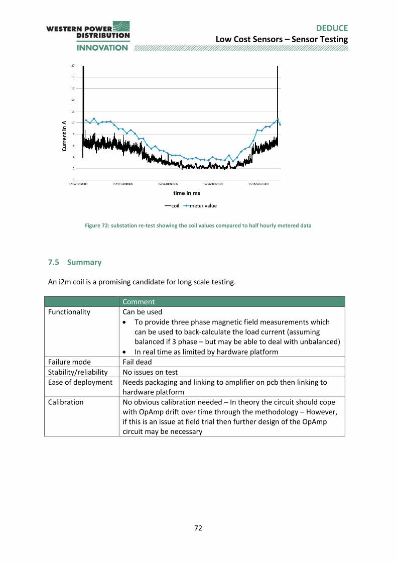
72
DEDUCE Low Cost Sensors – Sensor Testing
Figure 72: substation re-test showing the coil values compared to half hourly metered data
7.5 Summary An i2m coil is a promising candidate for long scale testing.
Comment
Functionality Can be used
To provide three phase magnetic field measurements which can be used to back-calculate the load current (assuming balanced if 3 phase – but may be able to deal with unbalanced)
In real time as limited by hardware platform
Failure mode Fail dead
Stability/reliability No issues on test
Ease of deployment Needs packaging and linking to amplifier on pcb then linking to hardware platform
Calibration No obvious calibration needed – In theory the circuit should cope with OpAmp drift over time through the methodology – However, if this is an issue at field trial then further design of the OpAmp circuit may be necessary
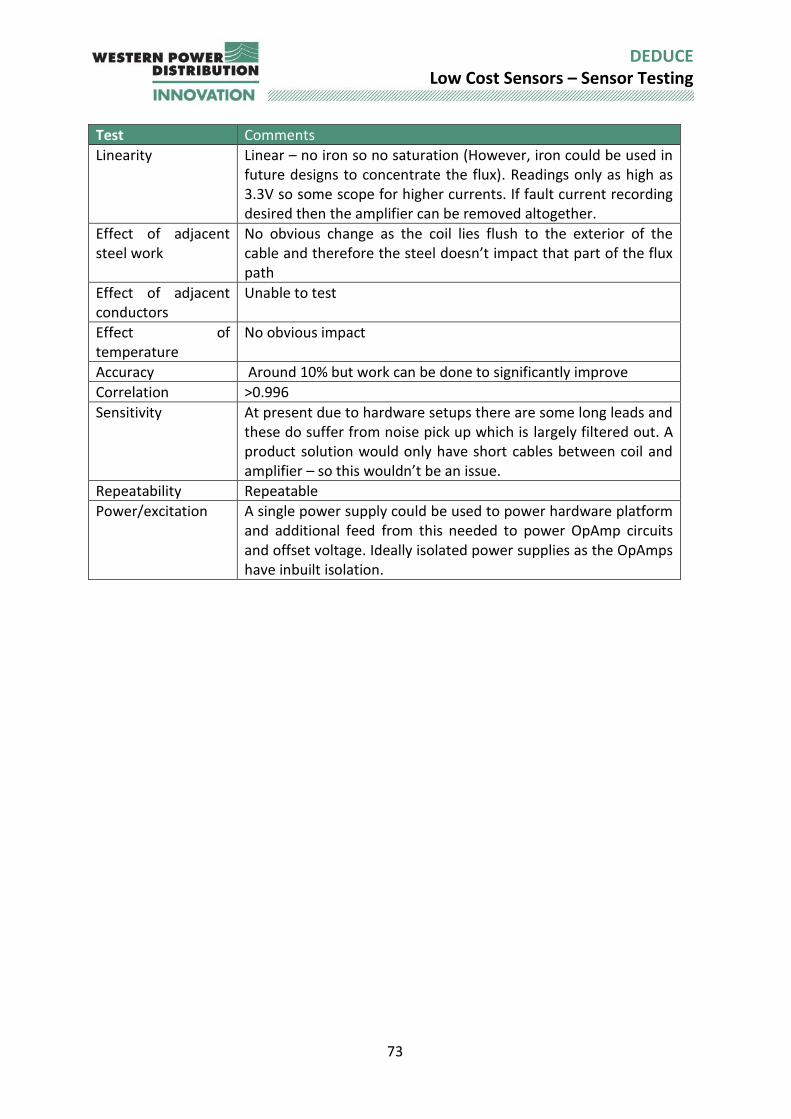
73
DEDUCE Low Cost Sensors – Sensor Testing
Test Comments
Linearity Linear – no iron so no saturation (However, iron could be used in future designs to concentrate the flux). Readings only as high as 3.3V so some scope for higher currents. If fault current recording desired then the amplifier can be removed altogether.
Effect of adjacent steel work
No obvious change as the coil lies flush to the exterior of the cable and therefore the steel doesn’t impact that part of the flux path
Effect of adjacent conductors
Unable to test
Effect of temperature
No obvious impact
Accuracy Around 10% but work can be done to significantly improve
Correlation >0.996
Sensitivity At present due to hardware setups there are some long leads and these do suffer from noise pick up which is largely filtered out. A product solution would only have short cables between coil and amplifier – so this wouldn’t be an issue.
Repeatability Repeatable
Power/excitation A single power supply could be used to power hardware platform and additional feed from this needed to power OpAmp circuits and offset voltage. Ideally isolated power supplies as the OpAmps have inbuilt isolation.
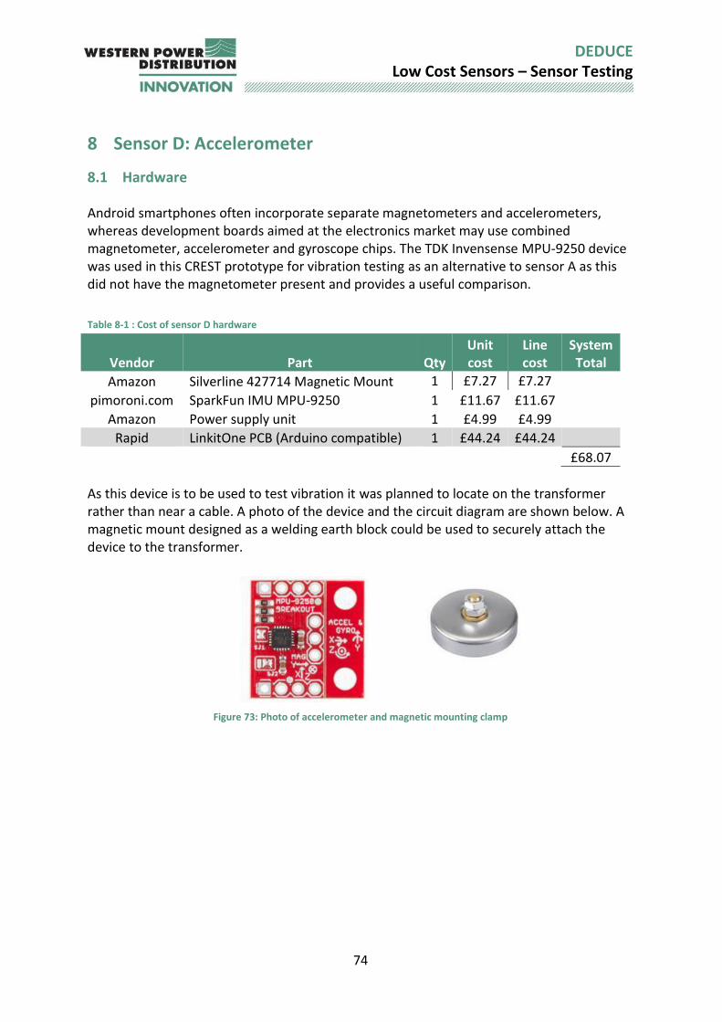
74
DEDUCE Low Cost Sensors – Sensor Testing
8 Sensor D: Accelerometer
8.1 Hardware Android smartphones often incorporate separate magnetometers and accelerometers, whereas development boards aimed at the electronics market may use combined magnetometer, accelerometer and gyroscope chips. The TDK Invensense MPU-9250 device was used in this CREST prototype for vibration testing as an alternative to sensor A as this did not have the magnetometer present and provides a useful comparison.
Table 8-1 : Cost of sensor D hardware
Vendor Part Qty Unit cost
Line cost
System Total
Amazon Silverline 427714 Magnetic Mount 1 £7.27 £7.27
pimoroni.com SparkFun IMU MPU-9250 1 £11.67 £11.67 Amazon Power supply unit 1 £4.99 £4.99
Rapid LinkitOne PCB (Arduino compatible) 1 £44.24 £44.24
£68.07
As this device is to be used to test vibration it was planned to locate on the transformer rather than near a cable. A photo of the device and the circuit diagram are shown below. A magnetic mount designed as a welding earth block could be used to securely attach the device to the transformer.
Figure 73: Photo of accelerometer and magnetic mounting clamp
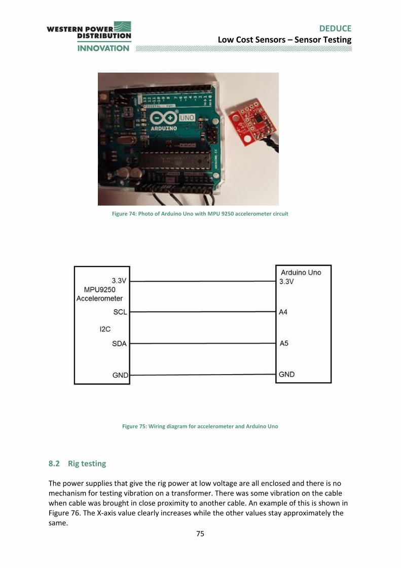
75
DEDUCE Low Cost Sensors – Sensor Testing
Figure 74: Photo of Arduino Uno with MPU 9250 accelerometer circuit
Figure 75: Wiring diagram for accelerometer and Arduino Uno
8.2 Rig testing The power supplies that give the rig power at low voltage are all enclosed and there is no mechanism for testing vibration on a transformer. There was some vibration on the cable when cable was brought in close proximity to another cable. An example of this is shown in Figure 76. The X-axis value clearly increases while the other values stay approximately the same.
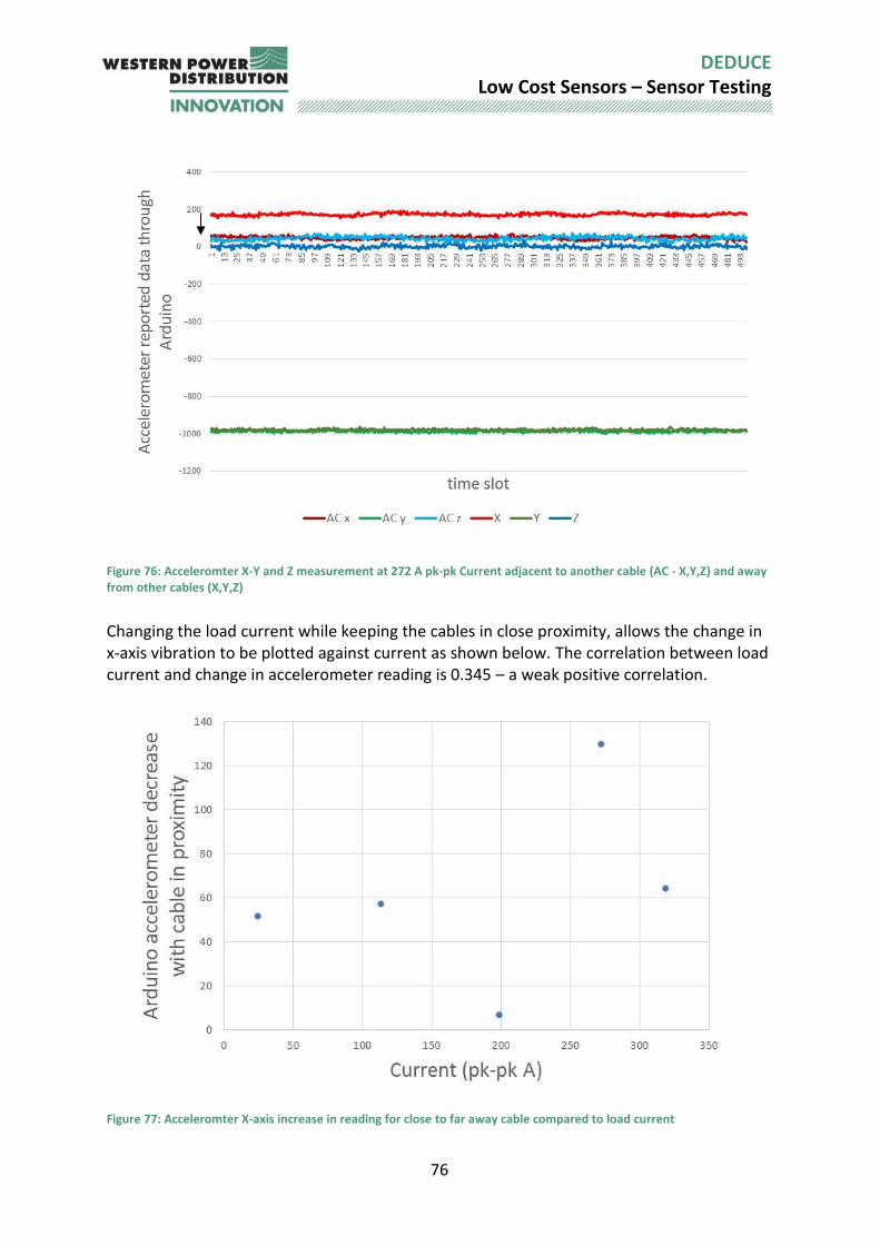
76
DEDUCE Low Cost Sensors – Sensor Testing
Figure 76: Acceleromter X-Y and Z measurement at 272 A pk-pk Current adjacent to another cable (AC - X,Y,Z) and away from other cables (X,Y,Z)
Changing the load current while keeping the cables in close proximity, allows the change in x-axis vibration to be plotted against current as shown below. The correlation between load current and change in accelerometer reading is 0.345 – a weak positive correlation.
Figure 77: Acceleromter X-axis increase in reading for close to far away cable compared to load current
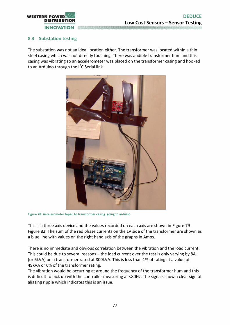
77
DEDUCE Low Cost Sensors – Sensor Testing
8.3 Substation testing The substation was not an ideal location either. The transformer was located within a thin steel casing which was not directly touching. There was audible transformer hum and this casing was vibrating so an accelerometer was placed on the transformer casing and hooked to an Arduino through the I2C Serial link.
Figure 78: Accelerometer taped to transformer casing going to arduino
This is a three axis device and the values recorded on each axis are shown in Figure 79-Figure 82. The sum of the red phase currents on the LV side of the transformer are shown as a blue line with values on the right hand axis of the graphs in Amps. There is no immediate and obvious correlation between the vibration and the load current. This could be due to several reasons – the load current over the test is only varying by 8A (or 6kVA) on a transformer rated at 800kVA. This is less than 1% of rating at a value of 49kVA or 6% of the transformer rating. The vibration would be occurring at around the frequency of the transformer hum and this is difficult to pick up with the controller measuring at <80Hz. The signals show a clear sign of aliasing ripple which indicates this is an issue.
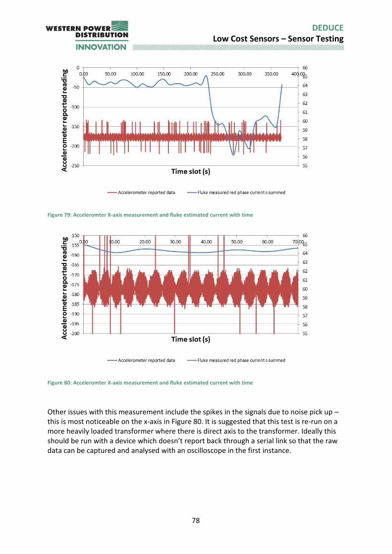
78
DEDUCE Low Cost Sensors – Sensor Testing
Figure 79: Acceleromter X-axis measurement and fluke estimated current with time
Figure 80: Acceleromter X-axis measurement and fluke estimated current with time
Other issues with this measurement include the spikes in the signals due to noise pick up – this is most noticeable on the x-axis in Figure 80. It is suggested that this test is re-run on a more heavily loaded transformer where there is direct axis to the transformer. Ideally this should be run with a device which doesn’t report back through a serial link so that the raw data can be captured and analysed with an oscilloscope in the first instance.

79
DEDUCE Low Cost Sensors – Sensor Testing
Figure 81: Acceleromter Y-axis measurement and fluke estimated current with time
Figure 82: Accelerometer z-axis measurement and fluke estimated current with time
LP 22 The testing undertaken indicated that it was not going to be possible to relate vibration with loading.
LP 23 Even if further testing proved there to be a relationship between loading and vibration under more highly loaded transformers it would require a significant amount of work to develop the maths and calibration process required for large scale roll out. It is unlikely that the calibration procedure could be achieved in a low enough time scale to keep the costs of installation below £50.
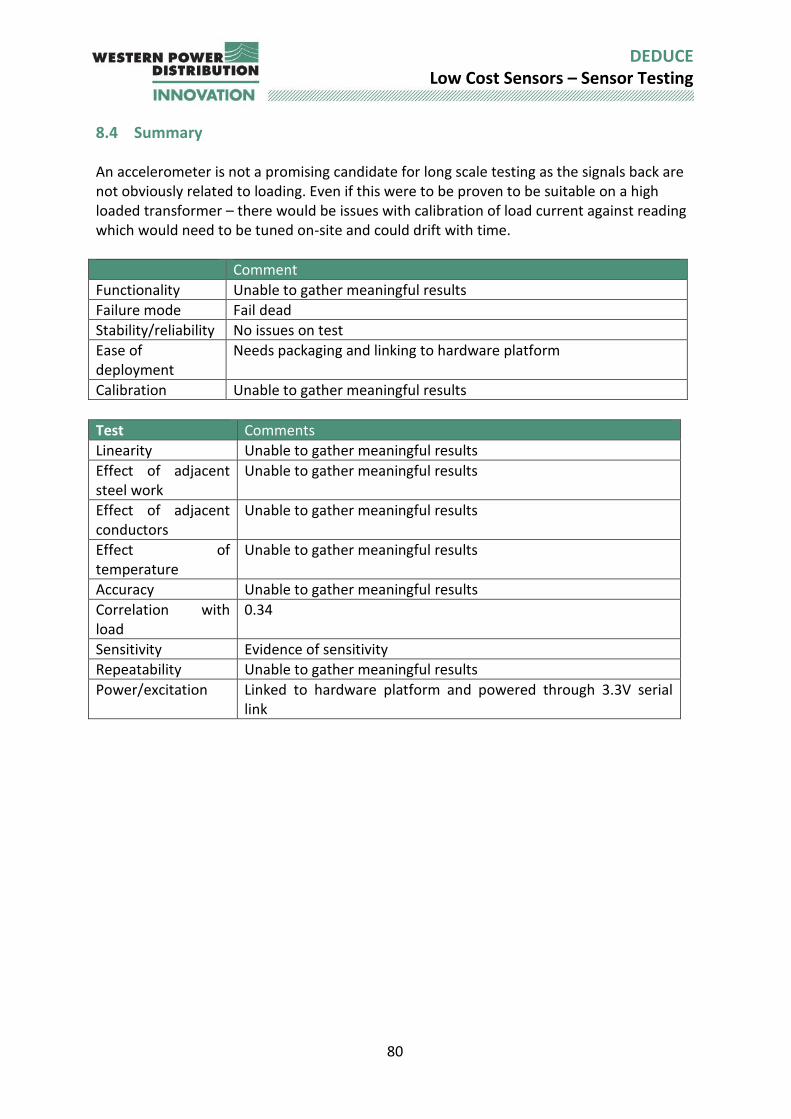
80
DEDUCE Low Cost Sensors – Sensor Testing
8.4 Summary An accelerometer is not a promising candidate for long scale testing as the signals back are not obviously related to loading. Even if this were to be proven to be suitable on a high loaded transformer – there would be issues with calibration of load current against reading which would need to be tuned on-site and could drift with time.
Comment
Functionality Unable to gather meaningful results
Failure mode Fail dead
Stability/reliability No issues on test
Ease of deployment
Needs packaging and linking to hardware platform
Calibration Unable to gather meaningful results
Test Comments
Linearity Unable to gather meaningful results
Effect of adjacent steel work
Unable to gather meaningful results
Effect of adjacent conductors
Unable to gather meaningful results
Effect of temperature
Unable to gather meaningful results
Accuracy Unable to gather meaningful results
Correlation with load
0.34
Sensitivity Evidence of sensitivity
Repeatability Unable to gather meaningful results
Power/excitation Linked to hardware platform and powered through 3.3V serial link
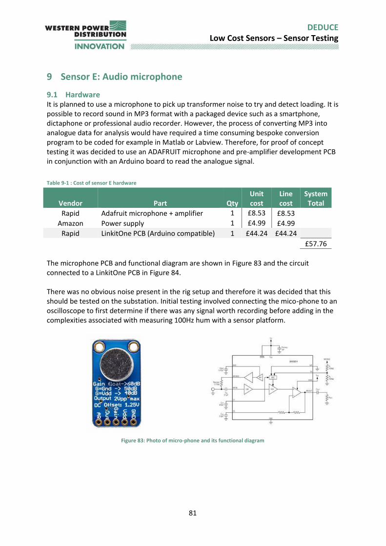
81
DEDUCE Low Cost Sensors – Sensor Testing
9 Sensor E: Audio microphone
9.1 Hardware It is planned to use a microphone to pick up transformer noise to try and detect loading. It is possible to record sound in MP3 format with a packaged device such as a smartphone, dictaphone or professional audio recorder. However, the process of converting MP3 into analogue data for analysis would have required a time consuming bespoke conversion program to be coded for example in Matlab or Labview. Therefore, for proof of concept testing it was decided to use an ADAFRUIT microphone and pre-amplifier development PCB in conjunction with an Arduino board to read the analogue signal.
Table 9-1 : Cost of sensor E hardware
Vendor Part Qty Unit cost
Line cost
System Total
Rapid Adafruit microphone + amplifier 1 £8.53 £8.53 Amazon Power supply 1 £4.99 £4.99
Rapid LinkitOne PCB (Arduino compatible) 1 £44.24 £44.24
£57.76
The microphone PCB and functional diagram are shown in Figure 83 and the circuit connected to a LinkitOne PCB in Figure 84. There was no obvious noise present in the rig setup and therefore it was decided that this should be tested on the substation. Initial testing involved connecting the mico-phone to an oscilloscope to first determine if there was any signal worth recording before adding in the complexities associated with measuring 100Hz hum with a sensor platform.
Figure 83: Photo of micro-phone and its functional diagram
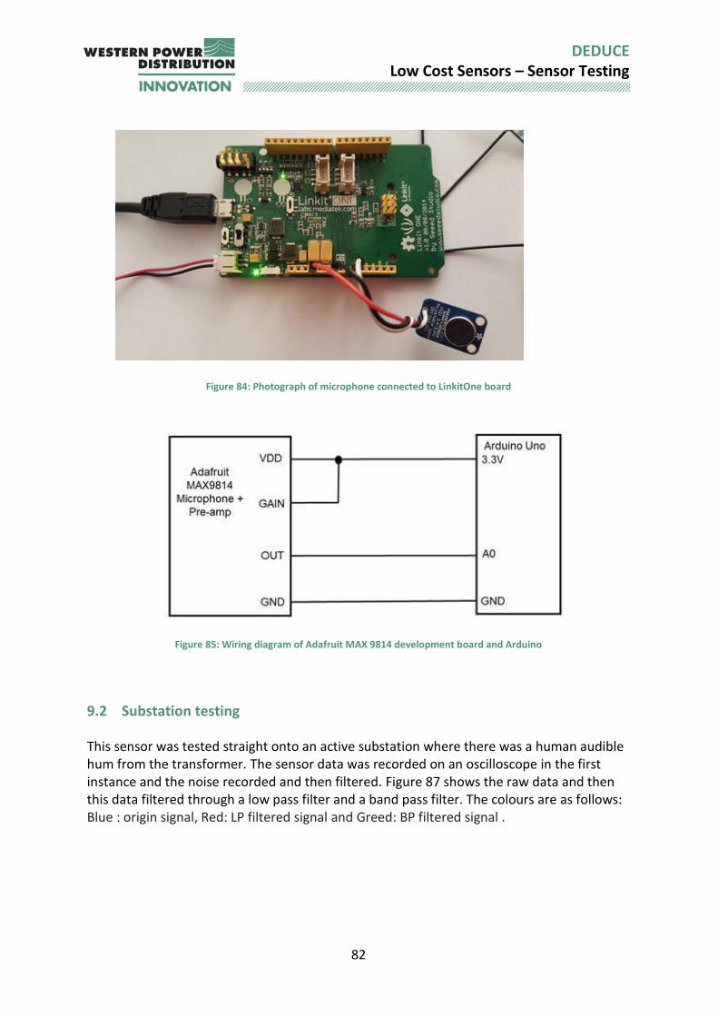
82
DEDUCE Low Cost Sensors – Sensor Testing
Figure 84: Photograph of microphone connected to LinkitOne board
Figure 85: Wiring diagram of Adafruit MAX 9814 development board and Arduino
9.2 Substation testing This sensor was tested straight onto an active substation where there was a human audible hum from the transformer. The sensor data was recorded on an oscilloscope in the first instance and the noise recorded and then filtered. Figure 87 shows the raw data and then this data filtered through a low pass filter and a band pass filter. The colours are as follows: Blue : origin signal, Red: LP filtered signal and Greed: BP filtered signal .
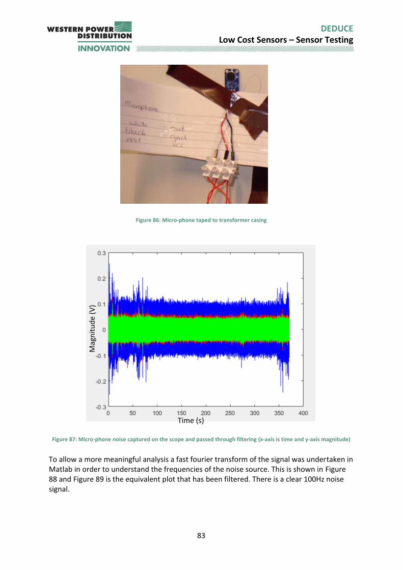
83
DEDUCE Low Cost Sensors – Sensor Testing
Figure 86: Micro-phone taped to transformer casing
Figure 87: Micro-phone noise captured on the scope and passed through filtering (x-axis is time and y-axis magnitude)
To allow a more meaningful analysis a fast fourier transform of the signal was undertaken in Matlab in order to understand the frequencies of the noise source. This is shown in Figure 88 and Figure 89 is the equivalent plot that has been filtered. There is a clear 100Hz noise signal.
Mag
nit
ud
e (V
)
Time (s)
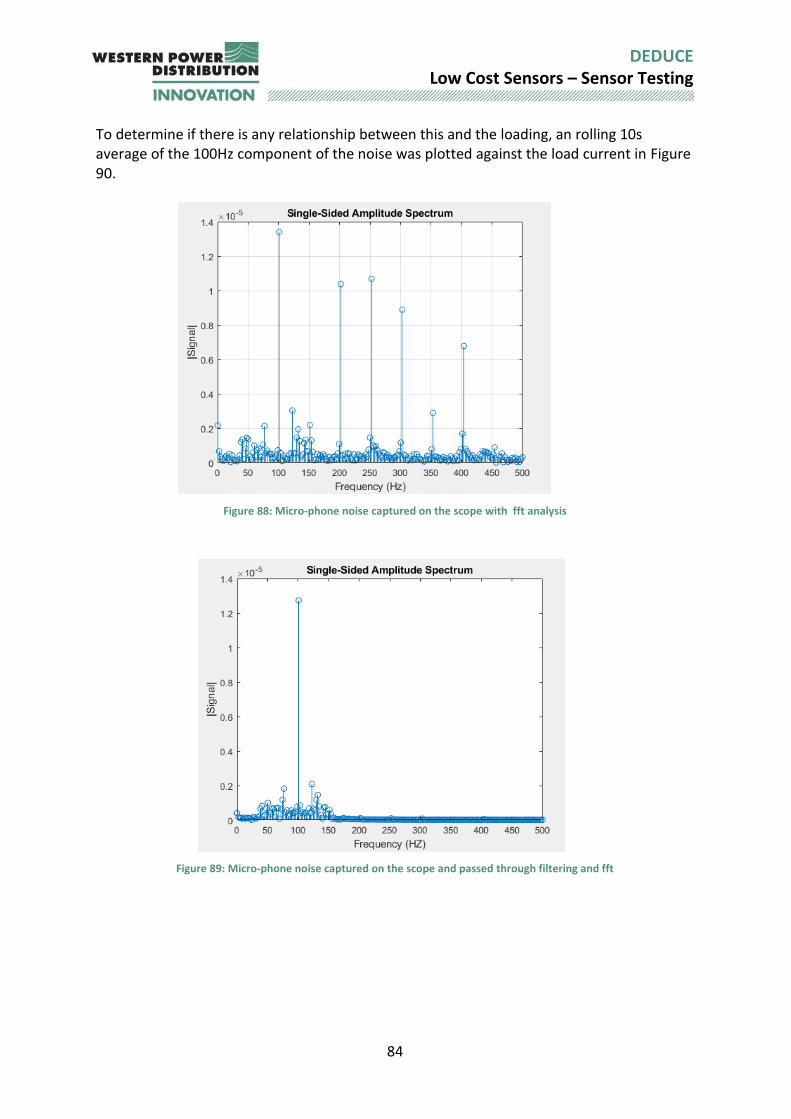
84
DEDUCE Low Cost Sensors – Sensor Testing
To determine if there is any relationship between this and the loading, an rolling 10s average of the 100Hz component of the noise was plotted against the load current in Figure 90.
Figure 88: Micro-phone noise captured on the scope with fft analysis
Figure 89: Micro-phone noise captured on the scope and passed through filtering and fft
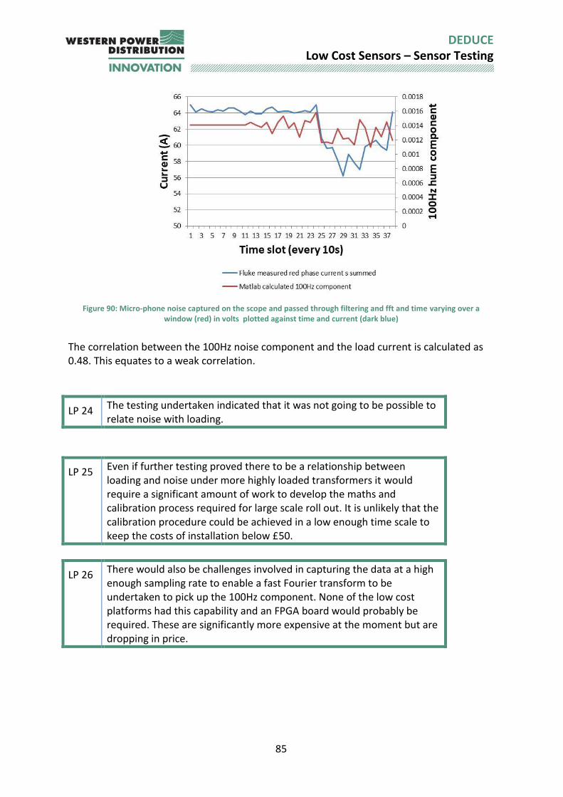
85
DEDUCE Low Cost Sensors – Sensor Testing
Figure 90: Micro-phone noise captured on the scope and passed through filtering and fft and time varying over a
window (red) in volts plotted against time and current (dark blue)
The correlation between the 100Hz noise component and the load current is calculated as 0.48. This equates to a weak correlation.
LP 24 The testing undertaken indicated that it was not going to be possible to relate noise with loading.
LP 25 Even if further testing proved there to be a relationship between loading and noise under more highly loaded transformers it would require a significant amount of work to develop the maths and calibration process required for large scale roll out. It is unlikely that the calibration procedure could be achieved in a low enough time scale to keep the costs of installation below £50.
LP 26 There would also be challenges involved in capturing the data at a high enough sampling rate to enable a fast Fourier transform to be undertaken to pick up the 100Hz component. None of the low cost platforms had this capability and an FPGA board would probably be required. These are significantly more expensive at the moment but are dropping in price.
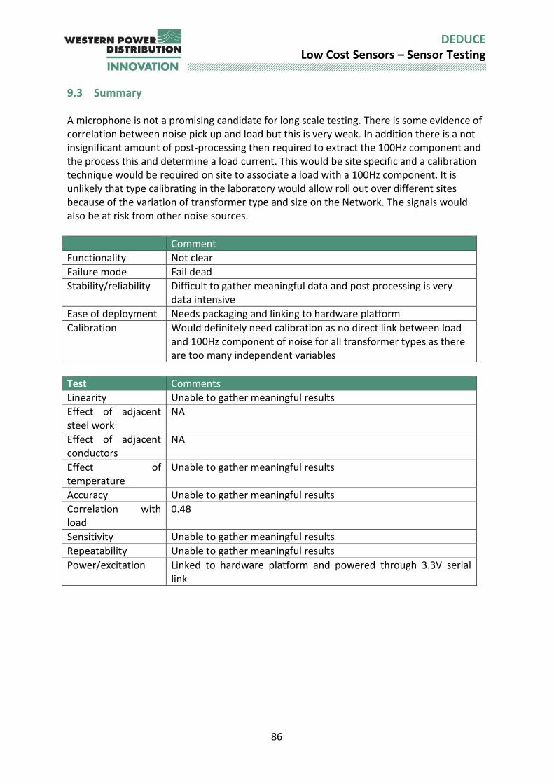
86
DEDUCE Low Cost Sensors – Sensor Testing
9.3 Summary A microphone is not a promising candidate for long scale testing. There is some evidence of correlation between noise pick up and load but this is very weak. In addition there is a not insignificant amount of post-processing then required to extract the 100Hz component and the process this and determine a load current. This would be site specific and a calibration technique would be required on site to associate a load with a 100Hz component. It is unlikely that type calibrating in the laboratory would allow roll out over different sites because of the variation of transformer type and size on the Network. The signals would also be at risk from other noise sources.
Comment
Functionality Not clear
Failure mode Fail dead
Stability/reliability Difficult to gather meaningful data and post processing is very data intensive
Ease of deployment Needs packaging and linking to hardware platform
Calibration Would definitely need calibration as no direct link between load and 100Hz component of noise for all transformer types as there are too many independent variables
Test Comments
Linearity Unable to gather meaningful results
Effect of adjacent steel work
NA
Effect of adjacent conductors
NA
Effect of temperature
Unable to gather meaningful results
Accuracy Unable to gather meaningful results
Correlation with load
0.48
Sensitivity Unable to gather meaningful results
Repeatability Unable to gather meaningful results
Power/excitation Linked to hardware platform and powered through 3.3V serial link
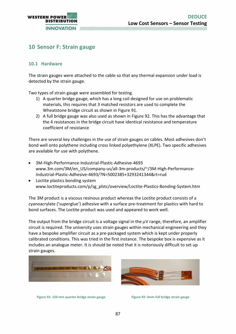
87
DEDUCE Low Cost Sensors – Sensor Testing
10 Sensor F: Strain gauge
10.1 Hardware The strain gauges were attached to the cable so that any thermal expansion under load is detected by the strain gauge. Two types of strain gauge were assembled for testing.
1) A quarter bridge gauge, which has a long coil designed for use on problematic materials, this requires that 3 matched resistors are used to complete the Wheatstone bridge circuit as shown in Figure 91.
2) A full bridge gauge was also used as shown in Figure 92. This has the advantage that the 4 resistances in the bridge circuit have identical resistance and temperature coefficient of resistance
There are several key challenges in the use of strain gauges on cables. Most adhesives don’t bond well onto polythene including cross linked polyethylene (XLPE). Two specific adhesives are available for use with polythene.
3M-High-Performance-Industrial-Plastic-Adhesive-4693 www.3m.com/3M/en_US/company-us/all-3m-products/~/3M-High-Performance-Industrial-Plastic-Adhesive-4693/?N=5002385+3293241344&rt=rud
Loctite plastics bonding system www.loctiteproducts.com/p/sg_plstc/overview/Loctite-Plastics-Bonding-System.htm
The 3M product is a viscous resinous product whereas the Loctite product consists of a cyanoacrylate (‘superglue’) adhesive with a surface pre-treatment for plastics with hard to bond surfaces. The Loctite product was used and appeared to work well.
The output from the bridge circuit is a voltage signal in the V range, therefore, an amplifier circuit is required. The university uses strain gauges within mechanical engineering and they have a bespoke amplifier circuit as a pre-packaged system which is kept under properly calibrated conditions. This was tried in the first instance. The bespoke box is expensive as it includes an analogue meter. It is should be noted that it is notoriously difficult to set up strain gauges.
Figure 91: 150 mm quarter bridge strain gauge Figure 92: 4mm full bridge strain gauge
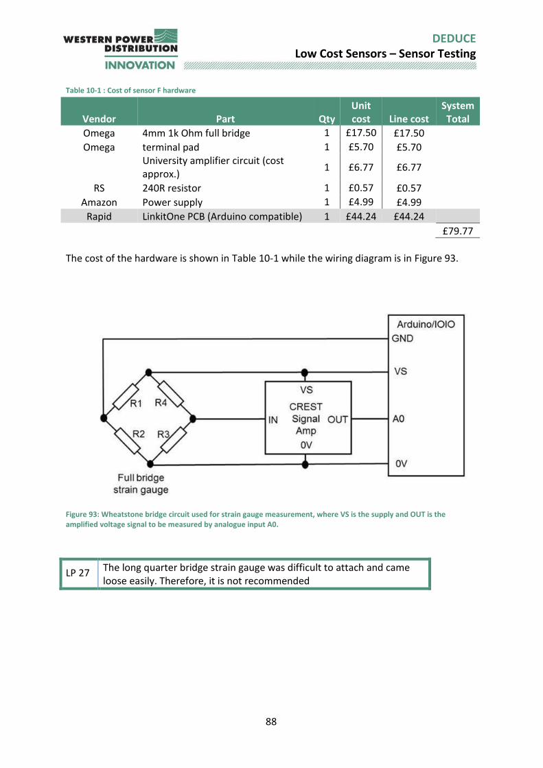
88
DEDUCE Low Cost Sensors – Sensor Testing
Table 10-1 : Cost of sensor F hardware
Vendor Part Qty Unit cost Line cost
System Total
Omega 4mm 1k Ohm full bridge 1 £17.50 £17.50 Omega terminal pad 1 £5.70 £5.70
University amplifier circuit (cost approx.)
1 £6.77 £6.77
RS 240R resistor 1 £0.57 £0.57 Amazon Power supply 1 £4.99 £4.99
Rapid LinkitOne PCB (Arduino compatible) 1 £44.24 £44.24 £79.77
The cost of the hardware is shown in Table 10-1 while the wiring diagram is in Figure 93.
Figure 93: Wheatstone bridge circuit used for strain gauge measurement, where VS is the supply and OUT is the amplified voltage signal to be measured by analogue input A0.
LP 27 The long quarter bridge strain gauge was difficult to attach and came loose easily. Therefore, it is not recommended
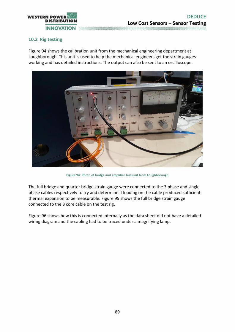
89
DEDUCE Low Cost Sensors – Sensor Testing
10.2 Rig testing Figure 94 shows the calibration unit from the mechanical engineering department at Loughborough. This unit is used to help the mechanical engineers get the strain gauges working and has detailed instructions. The output can also be sent to an oscilloscope.
Figure 94: Photo of bridge and amplifier test unit from Loughborough
The full bridge and quarter bridge strain gauge were connected to the 3 phase and single phase cables respectively to try and determine if loading on the cable produced sufficient thermal expansion to be measurable. Figure 95 shows the full bridge strain gauge connected to the 3 core cable on the test rig. Figure 96 shows how this is connected internally as the data sheet did not have a detailed wiring diagram and the cabling had to be traced under a magnifying lamp.
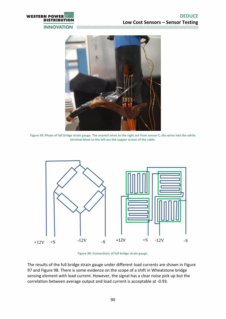
90
DEDUCE Low Cost Sensors – Sensor Testing
Figure 95: Photo of full bridge strain gauge. The enamel wires to the right are from sensor C, the wires into the white
terminal block to the left are the copper screen of the cable.
Figure 96: Connections of full bridge strain gauge.
The results of the full bridge strain gauge under different load currents are shown in Figure 97 and Figure 98. There is some evidence on the scope of a shift in Wheatstone bridge sensing element with load current. However, the signal has a clear noise pick up but the correlation between average output and load current is acceptable at -0.93.
+12V -12V +S -S +12V +S -12V -S
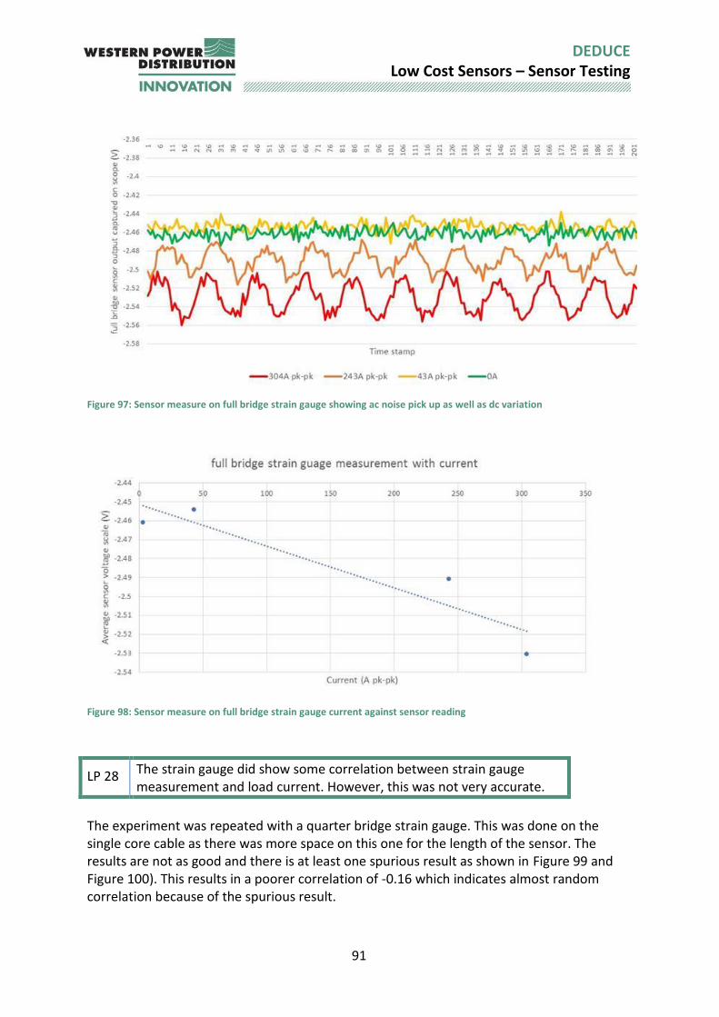
91
DEDUCE Low Cost Sensors – Sensor Testing
Figure 97: Sensor measure on full bridge strain gauge showing ac noise pick up as well as dc variation
Figure 98: Sensor measure on full bridge strain gauge current against sensor reading
LP 28 The strain gauge did show some correlation between strain gauge measurement and load current. However, this was not very accurate.
The experiment was repeated with a quarter bridge strain gauge. This was done on the single core cable as there was more space on this one for the length of the sensor. The results are not as good and there is at least one spurious result as shown in Figure 99 and Figure 100). This results in a poorer correlation of -0.16 which indicates almost random correlation because of the spurious result.
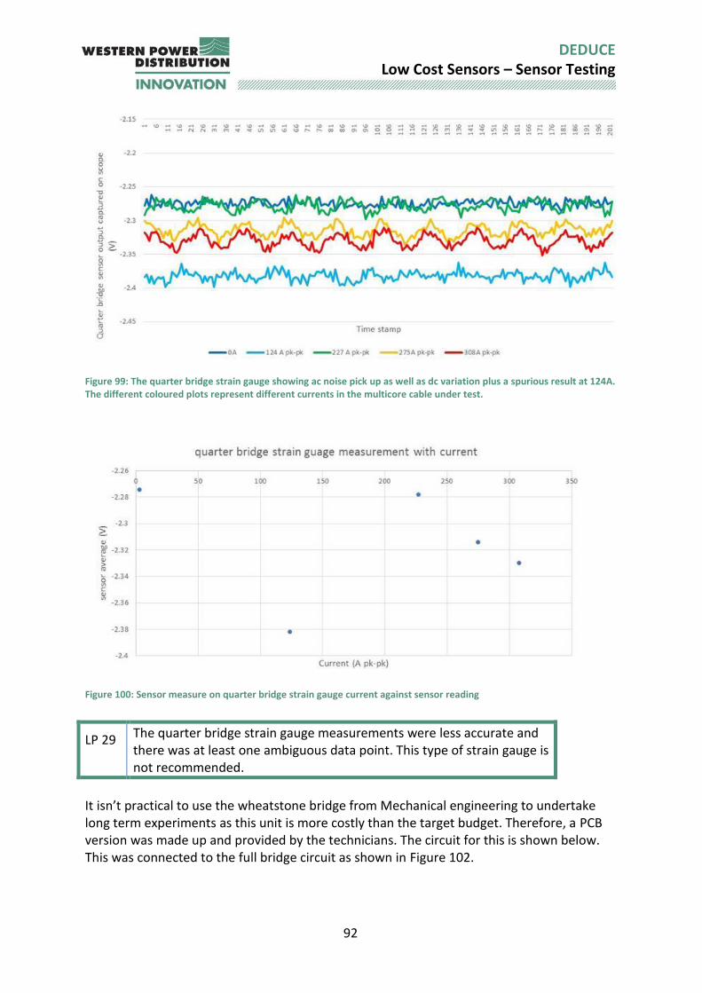
92
DEDUCE Low Cost Sensors – Sensor Testing
Figure 99: The quarter bridge strain gauge showing ac noise pick up as well as dc variation plus a spurious result at 124A. The different coloured plots represent different currents in the multicore cable under test.
Figure 100: Sensor measure on quarter bridge strain gauge current against sensor reading
LP 29 The quarter bridge strain gauge measurements were less accurate and there was at least one ambiguous data point. This type of strain gauge is not recommended.
It isn’t practical to use the wheatstone bridge from Mechanical engineering to undertake long term experiments as this unit is more costly than the target budget. Therefore, a PCB version was made up and provided by the technicians. The circuit for this is shown below. This was connected to the full bridge circuit as shown in Figure 102.
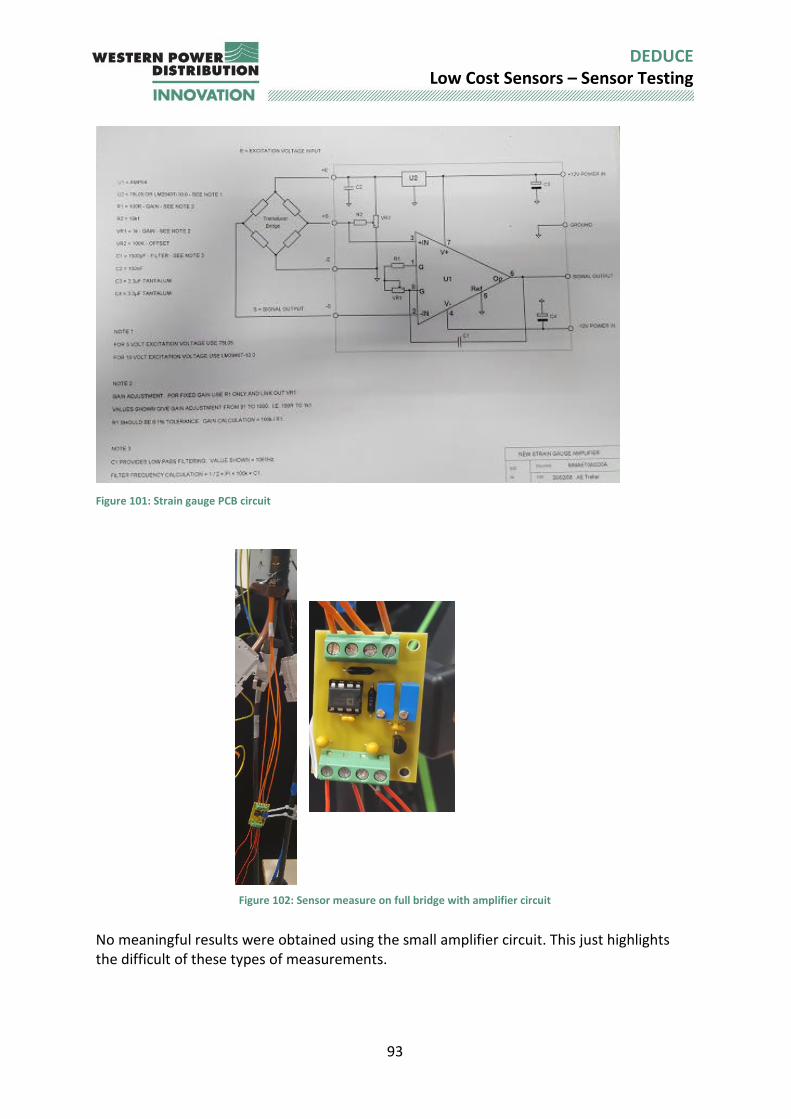
93
DEDUCE Low Cost Sensors – Sensor Testing
Figure 101: Strain gauge PCB circuit
Figure 102: Sensor measure on full bridge with amplifier circuit
No meaningful results were obtained using the small amplifier circuit. This just highlights the difficult of these types of measurements.

94
DEDUCE Low Cost Sensors – Sensor Testing
10.3 Summary A strain gauge is not a promising candidate for long scale testing.
Comment
Functionality Unlikely to be useful
Failure mode Fail dead
Stability/reliability Unstable values
Ease of deployment
Needs packaging and linking to hardware platform with Wheatstone bridge with variable resistors which would need setting up on site.
Calibration Difficult to do on site
Test Comments
Linearity Some evidence of linearity on test rig
Effect of adjacent steel work
NA
Effect of adjacent conductors
NA
Effect of temperature
A full bridge circuit is not impacted by temperature as this is compensated for. A half bridge circuit is.
Accuracy Estimated to be around 25% out at higher currents and worse at lower loading
Correlation with load current
-0.91
Sensitivity Overly sensitive
Repeatability Some repetition possible
Power/excitation Linked to hardware platform and Wheatstone bridge. The higher the supply voltage (within limits) the easier it is to see a reading. The output is also linked to an Amplifier which may be susceptible to OpAmp drift. The power requirements +/-12V are incompatible with low voltage consumer electronics so additional power conditioning would be needed.
95
DEDUCE Low Cost Sensors – Sensor Testing
11 Sensor G: Temperature sensors As current passes through a conductor it heats up due to I2R losses. Two approaches are investigated to detect this rise in temperature to try to relate back to load. The first is the ultra-low-cost approach of using temperature labels, traditionally used to alert technicians to a temperature problem during routine inspections. The second approach investigates the cost to transmit an over-temperature signal by GPRS. There are several issues that are important to consider when developing a measurement strategy. In many cases an indirect measurement leading to an inferred value may not be directly portable between different substation environments because of changes to hardware and other parameters that may be present in the system. An example of this is inferring transformer loading through transformer top oil temperature. In the WPD run FALCON project several distribution transformers were monitored over a year and the parameters used to tune a model of each transformer which could then be used to infer the loading based on the measured transformer top oil temperature and ambient temperature This process is complicated for several reasons;
There is a large variety in transformer size, type, manufacturer, year of manufacture etc so very few transformers are the same
There are three different models of a transformer that can be used. In FALCON the IEC60076 model provided a better correlation to the measured data and was deemed the most appropriate for use with the Distribution transformers under study.
The models rely on information which if not given (almost certainly not available) needs to be estimated through a calibration tuning process. This information includes; R (ratio of load losses at rated current to no load losses), ∆𝜃𝑜𝑟 the top oil temperature at rated load, 𝜏𝑜the oil time constant.
Fixing R to a typical value based on transformer size allows a real value of load to be used to tune the other two parameters using a weighted regression method
The method needed to be applied over the period of a week to tune the parameters but was then sufficiently accurate across the seasons.
The accuracy with which each top oil parameter could be calculated from loading data and ambient air temperature to check the tuned parameters was variable from <1% up to >5%
This then results in an onerous process of calibrating each transformer temperature measurement in situ. The data needs to be stored for a week and then analysed to allow the parameters to be tuned before being updated into a processor to allow for data values to be inferred. Any changes to the transformer (e.g. adding additional cooling) will result in the need for re-calibration. The measurement system is dependent on the ambient temperature, so this also needs to be recorded and used in the calculation. Wind and solar effects were indicated in work by EA Technology [29] to be negligible. As direct physical models are complex to produce, and many rely on detailed layout information. It is not practical to develop the sensors based purely on a theoretical
96
DEDUCE Low Cost Sensors – Sensor Testing
approach as the time necessary, for example, to calculate the magnetic field at any point due to 3D current flows is complex and time consuming and not likely to be accurate Therefore, a practical empirical method of calibrating sensors will be used.
LP 30 Calibrating a temperature measurement in one location with or without Utility found equipment does not guarantee calibration in other locations or with other pieces of equipment.
LP 31 Temperature calibration may change due to external influences such as temperature or over time.
11.1 Sensor G1: Thermal stickers/transducers Four main types of dynamic labels were procured for testing on live conductors:
1) Reversible temperature labels, which show the real-time temperature. 2) Irreversible temperature labels which show the maximum temperature which has
been reached 3) ‘Timestrip’ Time duration labels, which shows the duration since the label was
activated by pressing a button. 4) ‘Timestrip Plus’ Temperature duration labels which show the duration the label has
been at a given temperature The concept of this sensor type is that once the individual label types are proven, a combined label would be designed for use by DNOs or other electrical operation and maintenance (O&M) organisations which would include all 4 types in a single label, with temperatures optimised for electrical conductors and time durations optimised for DNO substation inspection regimes. At present this information is not automatically transmitted back to a central data store, but as the technology is very low cost – it is being investigated.
Table 11-1 : Cost of sensor G1 hardware
Vendor Part Qty Unit cost
Line cost
System Total
RS Temperature Label, 40°C to 71°C, 9 Level
1 £1.11 £1.11
RS Temperature Label 71°C to 110°C 1 £1.17 £1.17 Sigma Merck temperature duration label 2 1 £1.00 £1.00 Sigma Merck temperature duration label 3 1 £1.00 £1.00 £4.28
Leaving the stickers on the cable on the test rig yielded very little in the way of information. The tests being run were not at sufficiently high temperature to heat the cables and there was no changes to the label during the test runs. Eventually a hair dryer and a remote
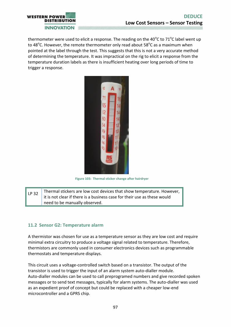
97
DEDUCE Low Cost Sensors – Sensor Testing
thermometer were used to elicit a response. The reading on the 40oC to 71oC label went up to 48oC. However, the remote thermometer only read about 58oC as a maximum when pointed at the label through the test. This suggests that this is not a very accurate method of determining the temperature. It was impractical on the rig to elicit a response from the temperature duration labels as there is insufficient heating over long periods of time to trigger a response.
Figure 103: Thermal sticker change after hairdryer
LP 32 Thermal stickers are low cost devices that show temperature. However, it is not clear if there is a business case for their use as these would need to be manually observed.
11.2 Sensor G2: Temperature alarm A thermistor was chosen for use as a temperature sensor as they are low cost and require minimal extra circuitry to produce a voltage signal related to temperature. Therefore, thermistors are commonly used in consumer electronics devices such as programmable thermostats and temperature displays. This circuit uses a voltage-controlled switch based on a transistor. The output of the transistor is used to trigger the input of an alarm system auto-dialler module. Auto-dialler modules can be used to call preprogramed numbers and give recorded spoken messages or to send text messages, typically for alarm systems. The auto-dialler was used as an expedient proof of concept but could be replaced with a cheaper low-end microcontroller and a GPRS chip.
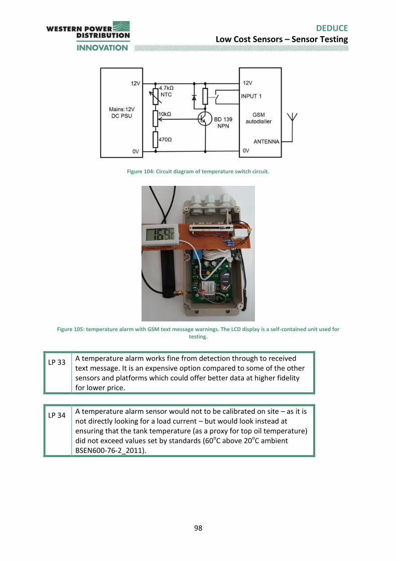
98
DEDUCE Low Cost Sensors – Sensor Testing
Figure 104: Circuit diagram of temperature switch circuit.
Figure 105: temperature alarm with GSM text message warnings. The LCD display is a self-contained unit used for
testing.
LP 33 A temperature alarm works fine from detection through to received text message. It is an expensive option compared to some of the other sensors and platforms which could offer better data at higher fidelity for lower price.
LP 34 A temperature alarm sensor would not to be calibrated on site – as it is not directly looking for a load current – but would look instead at ensuring that the tank temperature (as a proxy for top oil temperature) did not exceed values set by standards (60oC above 20oC ambient BSEN600-76-2_2011).
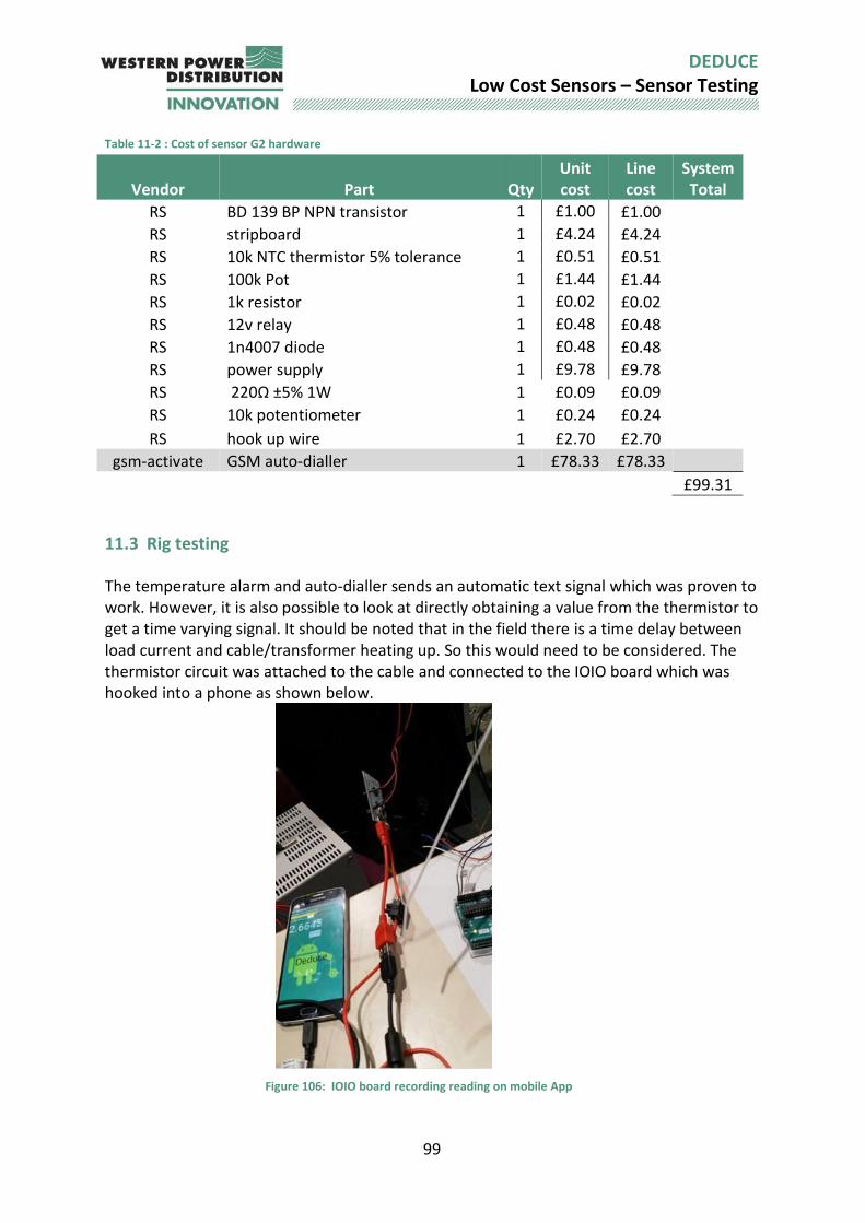
99
DEDUCE Low Cost Sensors – Sensor Testing
Table 11-2 : Cost of sensor G2 hardware
Vendor Part Qty Unit cost
Line cost
System Total
RS BD 139 BP NPN transistor 1 £1.00 £1.00 RS stripboard 1 £4.24 £4.24 RS 10k NTC thermistor 5% tolerance 1 £0.51 £0.51 RS 100k Pot 1 £1.44 £1.44 RS 1k resistor 1 £0.02 £0.02 RS 12v relay 1 £0.48 £0.48 RS 1n4007 diode 1 £0.48 £0.48 RS power supply 1 £9.78 £9.78 RS 220Ω ±5% 1W 1 £0.09 £0.09 RS 10k potentiometer 1 £0.24 £0.24 RS hook up wire 1 £2.70 £2.70 gsm-activate GSM auto-dialler 1 £78.33 £78.33 £99.31
11.3 Rig testing The temperature alarm and auto-dialler sends an automatic text signal which was proven to work. However, it is also possible to look at directly obtaining a value from the thermistor to get a time varying signal. It should be noted that in the field there is a time delay between load current and cable/transformer heating up. So this would need to be considered. The thermistor circuit was attached to the cable and connected to the IOIO board which was hooked into a phone as shown below.
Figure 106: IOIO board recording reading on mobile App
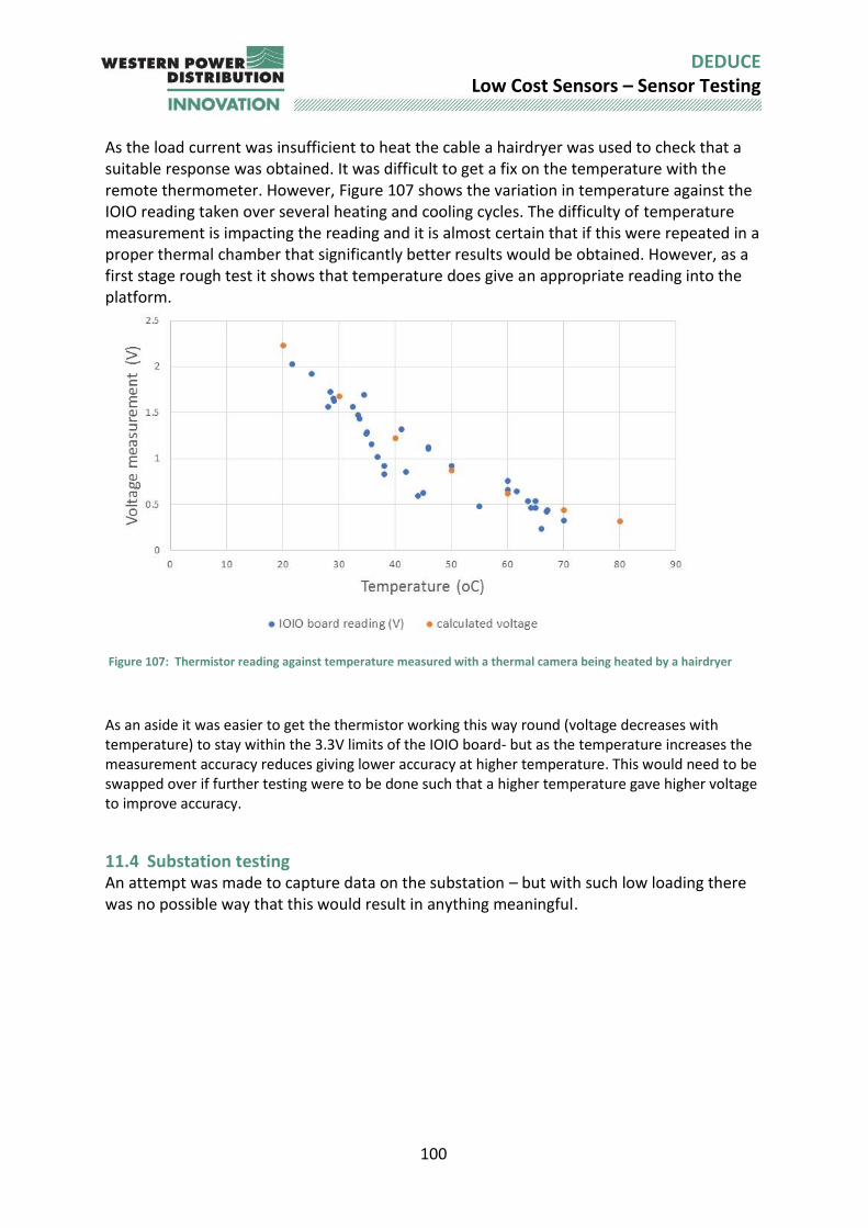
100
DEDUCE Low Cost Sensors – Sensor Testing
As the load current was insufficient to heat the cable a hairdryer was used to check that a suitable response was obtained. It was difficult to get a fix on the temperature with the remote thermometer. However, Figure 107 shows the variation in temperature against the IOIO reading taken over several heating and cooling cycles. The difficulty of temperature measurement is impacting the reading and it is almost certain that if this were repeated in a proper thermal chamber that significantly better results would be obtained. However, as a first stage rough test it shows that temperature does give an appropriate reading into the platform.
Figure 107: Thermistor reading against temperature measured with a thermal camera being heated by a hairdryer
As an aside it was easier to get the thermistor working this way round (voltage decreases with temperature) to stay within the 3.3V limits of the IOIO board- but as the temperature increases the measurement accuracy reduces giving lower accuracy at higher temperature. This would need to be swapped over if further testing were to be done such that a higher temperature gave higher voltage to improve accuracy.
11.4 Substation testing An attempt was made to capture data on the substation – but with such low loading there was no possible way that this would result in anything meaningful.
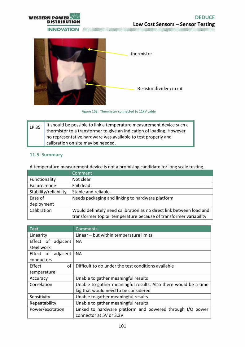
101
DEDUCE Low Cost Sensors – Sensor Testing
Figure 108: Thermistor connected to 11kV cable
LP 35 It should be possible to link a temperature measurement device such a thermistor to a transformer to give an indication of loading. However no representative hardware was available to test properly and calibration on site may be needed.
11.5 Summary A temperature measurement device is not a promising candidate for long scale testing.
Comment
Functionality Not clear
Failure mode Fail dead
Stability/reliability Stable and reliable
Ease of deployment
Needs packaging and linking to hardware platform
Calibration Would definitely need calibration as no direct link between load and transformer top oil temperature because of transformer variability
Test Comments
Linearity Linear – but within temperature limits
Effect of adjacent steel work
NA
Effect of adjacent conductors
NA
Effect of temperature
Difficult to do under the test conditions available
Accuracy Unable to gather meaningful results
Correlation Unable to gather meaningful results. Also there would be a time lag that would need to be considered
Sensitivity Unable to gather meaningful results
Repeatability Unable to gather meaningful results
Power/excitation Linked to hardware platform and powered through I/O power connector at 5V or 3.3V
thermistor
Resistor divider circuit
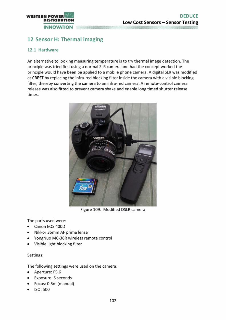
102
DEDUCE Low Cost Sensors – Sensor Testing
12 Sensor H: Thermal imaging
12.1 Hardware An alternative to looking measuring temperature is to try thermal image detection. The principle was tried first using a normal SLR camera and had the concept worked the principle would have been be applied to a mobile phone camera. A digital SLR was modified at CREST by replacing the infra-red blocking filter inside the camera with a visible blocking filter, thereby converting the camera to an infra-red camera. A remote-control camera release was also fitted to prevent camera shake and enable long timed shutter release times.
Figure 109: Modified DSLR camera
The parts used were:
Canon EOS 400D
Nikkor 35mm AF prime lense
YongNuo MC-36R wireless remote control
Visible light blocking filter Settings: The following settings were used on the camera:
Aperture: F5.6
Exposure: 5 seconds
Focus: 0.5m (manual)
ISO: 500
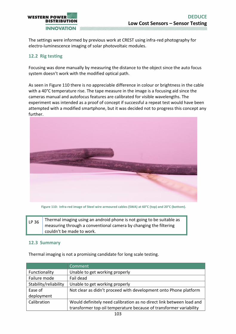
103
DEDUCE Low Cost Sensors – Sensor Testing
The settings were informed by previous work at CREST using infra-red photography for electro-luminescence imaging of solar photovoltaic modules.
12.2 Rig testing Focusing was done manually by measuring the distance to the object since the auto focus system doesn’t work with the modified optical path. As seen in Figure 110 there is no appreciable difference in colour or brightness in the cable with a 40°C temperature rise. The tape measure in the image is a focusing aid since the cameras manual and autofocus features are calibrated for visible wavelengths. The experiment was intended as a proof of concept if successful a repeat test would have been attempted with a modified smartphone, but it was decided not to progress this concept any further.
Figure 110: Infra-red image of Steel wire armoured cables (SWA) at 60°C (top) and 20°C (bottom).
LP 36 Thermal imaging using an android phone is not going to be suitable as measuring through a conventional camera by changing the filtering couldn’t be made to work.
12.3 Summary Thermal imaging is not a promising candidate for long scale testing.
Comment
Functionality Unable to get working properly
Failure mode Fail dead
Stability/reliability Unable to get working properly
Ease of deployment
Not clear as didn’t proceed with development onto Phone platform
Calibration Would definitely need calibration as no direct link between load and transformer top oil temperature because of transformer variability
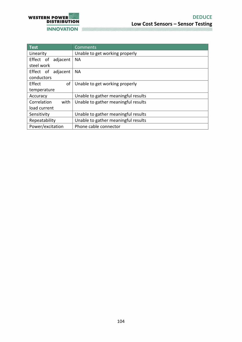
104
DEDUCE Low Cost Sensors – Sensor Testing
Test Comments
Linearity Unable to get working properly
Effect of adjacent steel work
NA
Effect of adjacent conductors
NA
Effect of temperature
Unable to get working properly
Accuracy Unable to gather meaningful results
Correlation with load current
Unable to gather meaningful results
Sensitivity Unable to gather meaningful results
Repeatability Unable to gather meaningful results
Power/excitation Phone cable connector
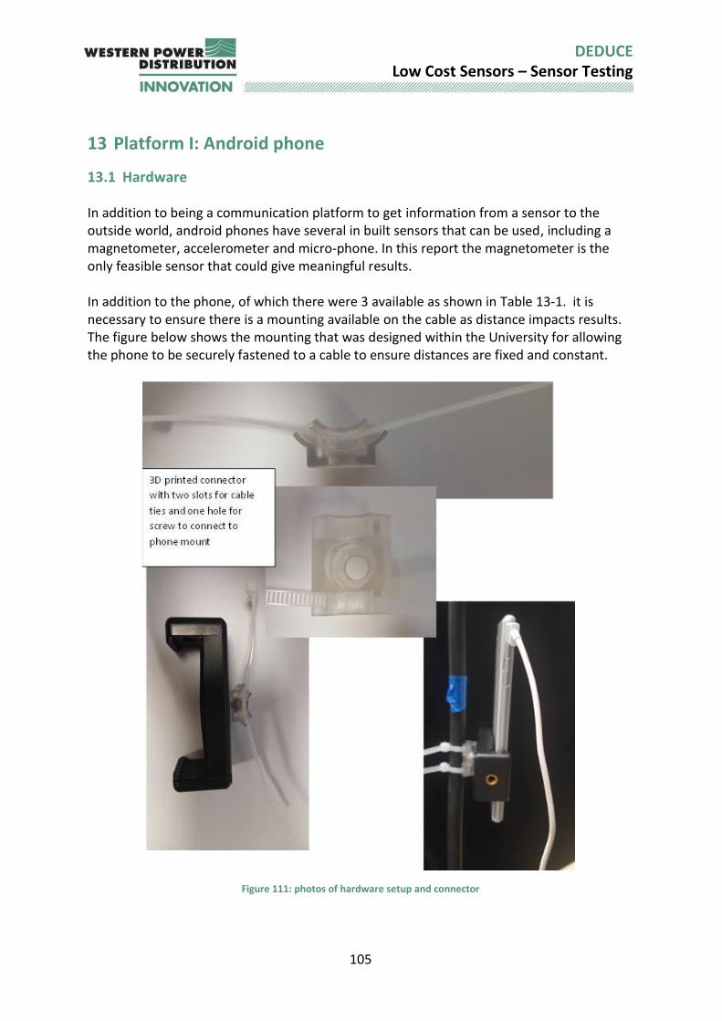
105
DEDUCE Low Cost Sensors – Sensor Testing
13 Platform I: Android phone
13.1 Hardware In addition to being a communication platform to get information from a sensor to the outside world, android phones have several in built sensors that can be used, including a magnetometer, accelerometer and micro-phone. In this report the magnetometer is the only feasible sensor that could give meaningful results. In addition to the phone, of which there were 3 available as shown in Table 13-1. it is necessary to ensure there is a mounting available on the cable as distance impacts results. The figure below shows the mounting that was designed within the University for allowing the phone to be securely fastened to a cable to ensure distances are fixed and constant.
Figure 111: photos of hardware setup and connector
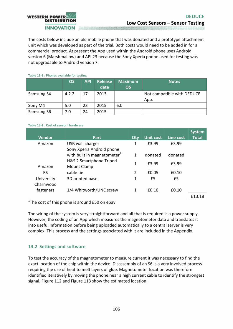
106
DEDUCE Low Cost Sensors – Sensor Testing
The costs below include an old mobile phone that was donated and a prototype attachment unit which was developed as part of the trial. Both costs would need to be added in for a commercial product. At present the App used within the Android phone uses Android version 6 (Marshmallow) and API 23 because the Sony Xperia phone used for testing was not upgradable to Android version 7.
Table 13-1 : Phones available for testing
OS API Release date
Maximum OS
Notes
Samsung S4 4.2.2 17 2013 Not compatible with DEDUCE App.
Sony M4 5.0 23 2015 6.0
Samsung S6 7.0 24 2015
Table 13-2 : Cost of sensor I hardware
Vendor Part Qty Unit cost Line cost System Total
Amazon USB wall charger 1 £3.99 £3.99
Sony Xperia Android phone with built in magnetometer1 1 donated donated
Amazon
H&S 2 Smartphone Tripod Mount Clamp
1 £3.99 £3.99
RS cable tie 2 £0.05 £0.10 University 3D printed base 1 £5 £5 Charnwood
fasteners 1/4 Whitworth/UNC screw 1 £0.10 £0.10 £13.18
1The cost of this phone is around £50 on ebay The wiring of the system is very straightforward and all that is required is a power supply. However, the coding of an App which measures the magnetometer data and translates it into useful information before being uploaded automatically to a central server is very complex. This process and the settings associated with it are included in the Appendix.
13.2 Settings and software To test the accuracy of the magnetometer to measure current it was necessary to find the exact location of the chip within the device. Disassembly of an S6 is a very involved process requiring the use of heat to melt layers of glue. Magnetometer location was therefore identified iteratively by moving the phone near a high current cable to identify the strongest signal. Figure 112 and Figure 113 show the estimated location.

107
DEDUCE Low Cost Sensors – Sensor Testing
Figure 112 : Photograph of Samsung S6 with the approximate position of the magnetometer marked with a red arrow.
Figure 113 : Photograph showing Samsung S6 Main PCB with the approximate position of the magnetometer marked with a red arrow.
LP 37 Distance is a factor when turning magnetic field back to an estimate of load current. Therefore, the location of the sensor is important to estimate its distance from the centre of the cable.
The android API provides two sets of variables for app programmers can access
‘Uncalibrated’ which in fact is calibrated both for factory tolerances in the sensors sensitivity and transient changes in sensor sensitivity due to device temperature. This also includes a calibration factor for factors such as manufacturing tolerances and interference from metal components in the phone.
‘Calibrated’ which is compensated for so called hard-iron losses, which might change for example if the user puts the phone in a case with a magnetic latch. This calibration is done automatically by the device when sufficient device movement is detected.
User advice is to move the phone in a figure of eight motion when the phone requires calibration. Fundamentally the device needs to be rotated 360° in all three axes to recalibrate it.
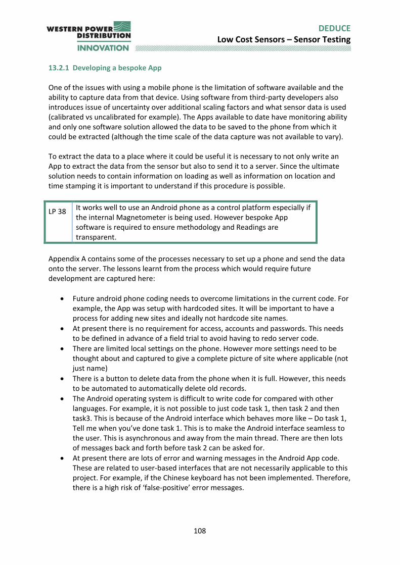
108
DEDUCE Low Cost Sensors – Sensor Testing
13.2.1 Developing a bespoke App One of the issues with using a mobile phone is the limitation of software available and the ability to capture data from that device. Using software from third-party developers also introduces issue of uncertainty over additional scaling factors and what sensor data is used (calibrated vs uncalibrated for example). The Apps available to date have monitoring ability and only one software solution allowed the data to be saved to the phone from which it could be extracted (although the time scale of the data capture was not available to vary). To extract the data to a place where it could be useful it is necessary to not only write an App to extract the data from the sensor but also to send it to a server. Since the ultimate solution needs to contain information on loading as well as information on location and time stamping it is important to understand if this procedure is possible.
LP 38 It works well to use an Android phone as a control platform especially if the internal Magnetometer is being used. However bespoke App software is required to ensure methodology and Readings are transparent.
Appendix A contains some of the processes necessary to set up a phone and send the data onto the server. The lessons learnt from the process which would require future development are captured here:
Future android phone coding needs to overcome limitations in the current code. For example, the App was setup with hardcoded sites. It will be important to have a process for adding new sites and ideally not hardcode site names.
At present there is no requirement for access, accounts and passwords. This needs to be defined in advance of a field trial to avoid having to redo server code.
There are limited local settings on the phone. However more settings need to be thought about and captured to give a complete picture of site where applicable (not just name)
There is a button to delete data from the phone when it is full. However, this needs to be automated to automatically delete old records.
The Android operating system is difficult to write code for compared with other languages. For example, it is not possible to just code task 1, then task 2 and then task3. This is because of the Android interface which behaves more like – Do task 1, Tell me when you’ve done task 1. This is to make the Android interface seamless to the user. This is asynchronous and away from the main thread. There are then lots of messages back and forth before task 2 can be asked for.
At present there are lots of error and warning messages in the Android App code. These are related to user-based interfaces that are not necessarily applicable to this project. For example, if the Chinese keyboard has not been implemented. Therefore, there is a high risk of ‘false-positive’ error messages.
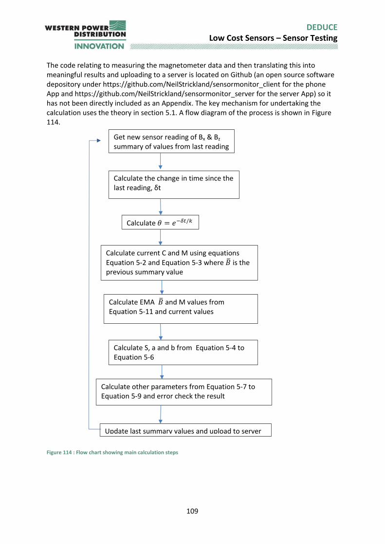
109
DEDUCE Low Cost Sensors – Sensor Testing
The code relating to measuring the magnetometer data and then translating this into meaningful results and uploading to a server is located on Github (an open source software depository under https://github.com/NeilStrickland/sensormonitor_client for the phone App and https://github.com/NeilStrickland/sensormonitor_server for the server App) so it has not been directly included as an Appendix. The key mechanism for undertaking the calculation uses the theory in section 5.1. A flow diagram of the process is shown in Figure 114.
Figure 114 : Flow chart showing main calculation steps
Get new sensor reading of Bx & Bz
summary of values from last reading
Calculate the change in time since the last reading, δt
Calculate 𝜃 = 𝑒−𝛿𝑡/𝑘
Calculate current C and M using equations Equation 5-2 and Equation 5-3 where �� is the previous summary value
Calculate EMA �� and M values from Equation 5-11 and current values
Calculate S, a and b from Equation 5-4 to Equation 5-6
Calculate other parameters from Equation 5-7 to Equation 5-9 and error check the result
Update last summary values and upload to server
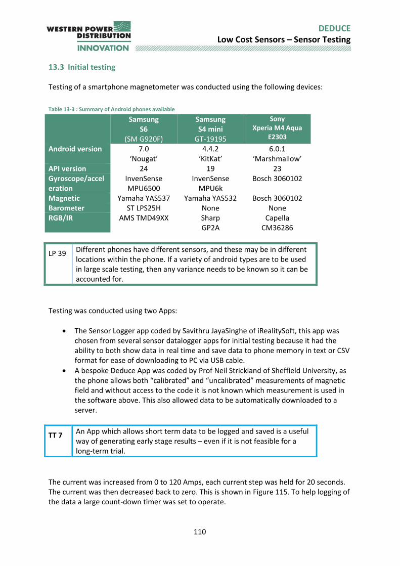
110
DEDUCE Low Cost Sensors – Sensor Testing
13.3 Initial testing Testing of a smartphone magnetometer was conducted using the following devices:
Table 13-3 : Summary of Android phones available
Samsung S6
(SM G920F)
Samsung S4 mini
GT-19195
Sony Xperia M4 Aqua
E2303
Android version 7.0 ‘Nougat’
4.4.2 ‘KitKat’
6.0.1 ‘Marshmallow’
API version 24 19 23 Gyroscope/acceleration
InvenSense MPU6500
InvenSense MPU6k
Bosch 3060102
Magnetic Yamaha YAS537 Yamaha YAS532 Bosch 3060102 Barometer ST LPS25H None None RGB/IR AMS TMD49XX Sharp
GP2A Capella
CM36286
LP 39 Different phones have different sensors, and these may be in different locations within the phone. If a variety of android types are to be used in large scale testing, then any variance needs to be known so it can be accounted for.
Testing was conducted using two Apps:
The Sensor Logger app coded by Savithru JayaSinghe of iRealitySoft, this app was chosen from several sensor datalogger apps for initial testing because it had the ability to both show data in real time and save data to phone memory in text or CSV format for ease of downloading to PC via USB cable.
A bespoke Deduce App was coded by Prof Neil Strickland of Sheffield University, as the phone allows both “calibrated” and “uncalibrated” measurements of magnetic field and without access to the code it is not known which measurement is used in the software above. This also allowed data to be automatically downloaded to a server.
TT 7
An App which allows short term data to be logged and saved is a useful way of generating early stage results – even if it is not feasible for a long-term trial.
The current was increased from 0 to 120 Amps, each current step was held for 20 seconds. The current was then decreased back to zero. This is shown in Figure 115. To help logging of the data a large count-down timer was set to operate.
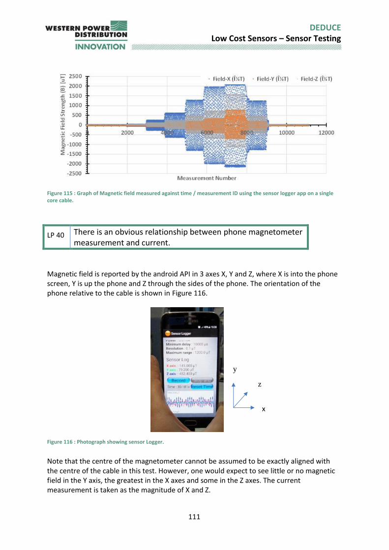
111
DEDUCE Low Cost Sensors – Sensor Testing
Figure 115 : Graph of Magnetic field measured against time / measurement ID using the sensor logger app on a single core cable.
LP 40 There is an obvious relationship between phone magnetometer measurement and current.
Magnetic field is reported by the android API in 3 axes X, Y and Z, where X is into the phone screen, Y is up the phone and Z through the sides of the phone. The orientation of the phone relative to the cable is shown in Figure 116.
Figure 116 : Photograph showing sensor Logger.
Note that the centre of the magnetometer cannot be assumed to be exactly aligned with the centre of the cable in this test. However, one would expect to see little or no magnetic field in the Y axis, the greatest in the X axes and some in the Z axes. The current measurement is taken as the magnitude of X and Z.
x
y
z
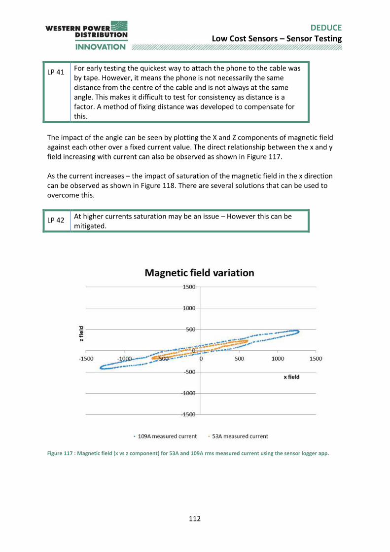
112
DEDUCE Low Cost Sensors – Sensor Testing
LP 41 For early testing the quickest way to attach the phone to the cable was by tape. However, it means the phone is not necessarily the same distance from the centre of the cable and is not always at the same angle. This makes it difficult to test for consistency as distance is a factor. A method of fixing distance was developed to compensate for this.
The impact of the angle can be seen by plotting the X and Z components of magnetic field against each other over a fixed current value. The direct relationship between the x and y field increasing with current can also be observed as shown in Figure 117. As the current increases – the impact of saturation of the magnetic field in the x direction can be observed as shown in Figure 118. There are several solutions that can be used to overcome this.
LP 42 At higher currents saturation may be an issue – However this can be mitigated.
Figure 117 : Magnetic field (x vs z component) for 53A and 109A rms measured current using the sensor logger app.
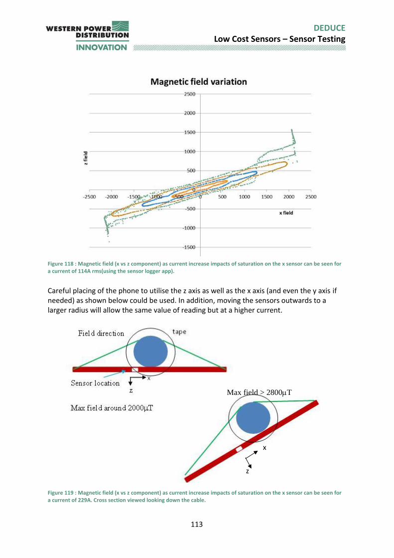
113
DEDUCE Low Cost Sensors – Sensor Testing
Figure 118 : Magnetic field (x vs z component) as current increase impacts of saturation on the x sensor can be seen for a current of 114A rms(using the sensor logger app).
Careful placing of the phone to utilise the z axis as well as the x axis (and even the y axis if needed) as shown below could be used. In addition, moving the sensors outwards to a larger radius will allow the same value of reading but at a higher current.
Figure 119 : Magnetic field (x vs z component) as current increase impacts of saturation on the x sensor can be seen for a current of 229A. Cross section viewed looking down the cable.
Max field > 2800T
x
z
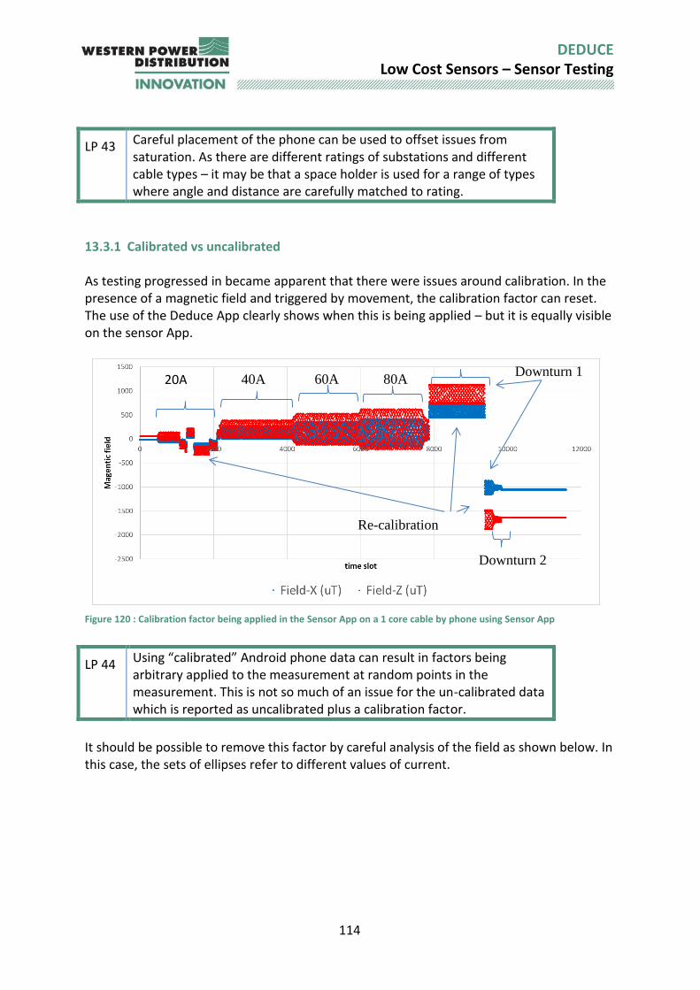
114
DEDUCE Low Cost Sensors – Sensor Testing
LP 43 Careful placement of the phone can be used to offset issues from saturation. As there are different ratings of substations and different cable types – it may be that a space holder is used for a range of types where angle and distance are carefully matched to rating.
13.3.1 Calibrated vs uncalibrated As testing progressed in became apparent that there were issues around calibration. In the presence of a magnetic field and triggered by movement, the calibration factor can reset. The use of the Deduce App clearly shows when this is being applied – but it is equally visible on the sensor App.
Figure 120 : Calibration factor being applied in the Sensor App on a 1 core cable by phone using Sensor App
LP 44 Using “calibrated” Android phone data can result in factors being arbitrary applied to the measurement at random points in the measurement. This is not so much of an issue for the un-calibrated data which is reported as uncalibrated plus a calibration factor.
It should be possible to remove this factor by careful analysis of the field as shown below. In this case, the sets of ellipses refer to different values of current.
20A 40A 60A 80A Downturn 1
Downturn 2
Re-calibration
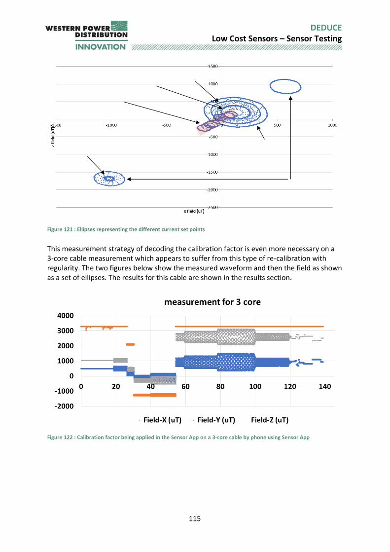
115
DEDUCE Low Cost Sensors – Sensor Testing
Figure 121 : Ellipses representing the different current set points
This measurement strategy of decoding the calibration factor is even more necessary on a 3-core cable measurement which appears to suffer from this type of re-calibration with regularity. The two figures below show the measured waveform and then the field as shown as a set of ellipses. The results for this cable are shown in the results section.
Figure 122 : Calibration factor being applied in the Sensor App on a 3-core cable by phone using Sensor App
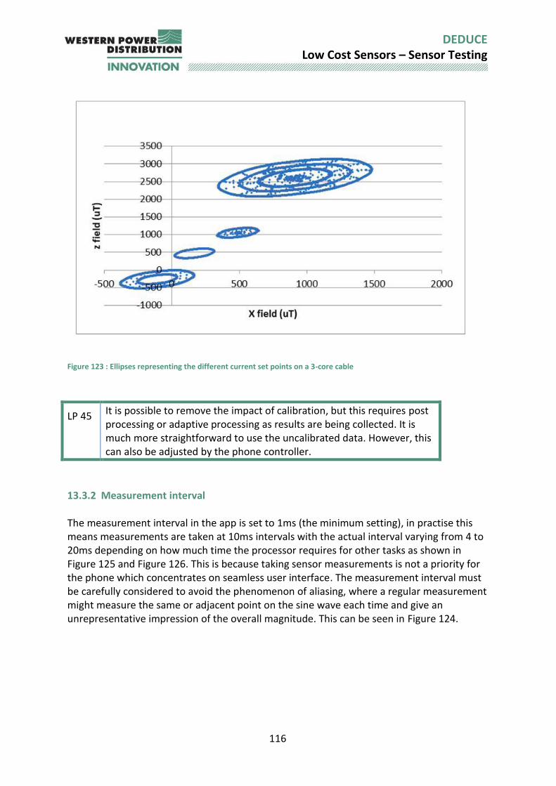
116
DEDUCE Low Cost Sensors – Sensor Testing
Figure 123 : Ellipses representing the different current set points on a 3-core cable
LP 45 It is possible to remove the impact of calibration, but this requires post processing or adaptive processing as results are being collected. It is much more straightforward to use the uncalibrated data. However, this can also be adjusted by the phone controller.
13.3.2 Measurement interval The measurement interval in the app is set to 1ms (the minimum setting), in practise this means measurements are taken at 10ms intervals with the actual interval varying from 4 to 20ms depending on how much time the processor requires for other tasks as shown in Figure 125 and Figure 126. This is because taking sensor measurements is not a priority for the phone which concentrates on seamless user interface. The measurement interval must be carefully considered to avoid the phenomenon of aliasing, where a regular measurement might measure the same or adjacent point on the sine wave each time and give an unrepresentative impression of the overall magnitude. This can be seen in Figure 124.
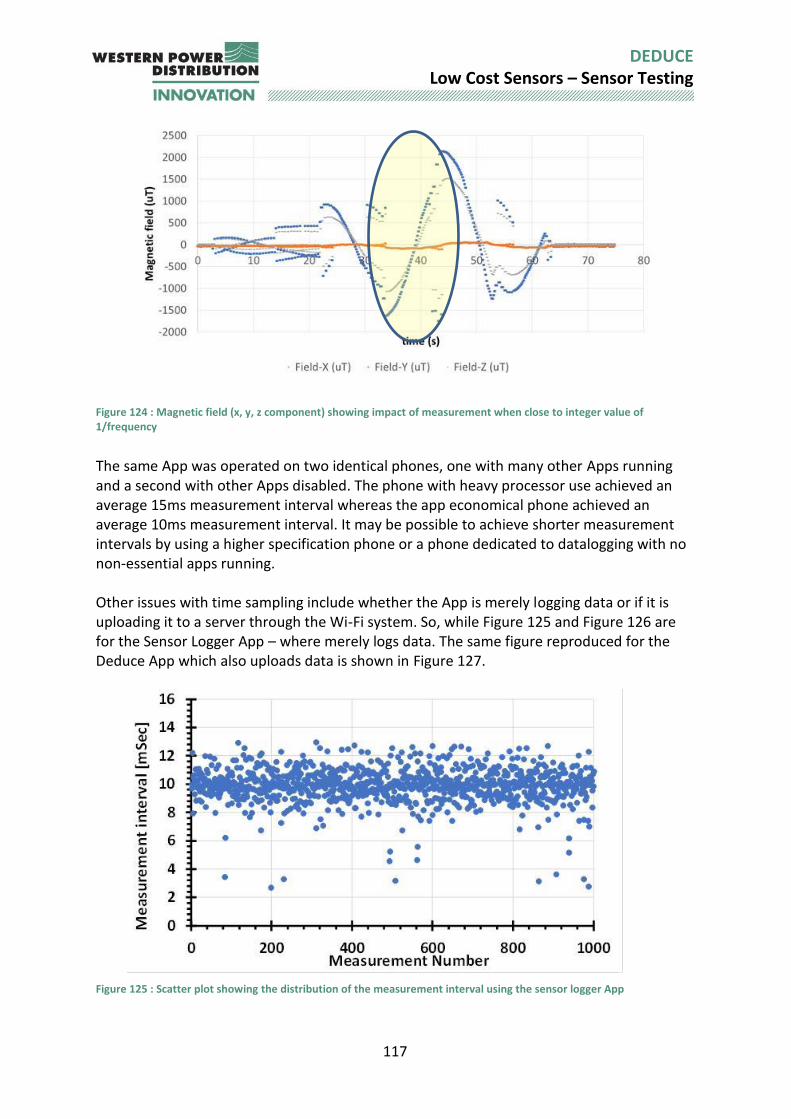
117
DEDUCE Low Cost Sensors – Sensor Testing
Figure 124 : Magnetic field (x, y, z component) showing impact of measurement when close to integer value of 1/frequency
The same App was operated on two identical phones, one with many other Apps running and a second with other Apps disabled. The phone with heavy processor use achieved an average 15ms measurement interval whereas the app economical phone achieved an average 10ms measurement interval. It may be possible to achieve shorter measurement intervals by using a higher specification phone or a phone dedicated to datalogging with no non-essential apps running. Other issues with time sampling include whether the App is merely logging data or if it is uploading it to a server through the Wi-Fi system. So, while Figure 125 and Figure 126 are for the Sensor Logger App – where merely logs data. The same figure reproduced for the Deduce App which also uploads data is shown in Figure 127.
Figure 125 : Scatter plot showing the distribution of the measurement interval using the sensor logger App
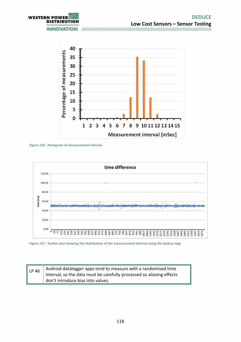
118
DEDUCE Low Cost Sensors – Sensor Testing
Figure 126 : Histogram of measurement interval.
Figure 127 : Scatter plot showing the distribution of the measurement interval using the deduce App
LP 46 Android datalogger apps tend to measure with a randomised time interval, so the data must be carefully processed so aliasing effects don’t introduce bias into values.
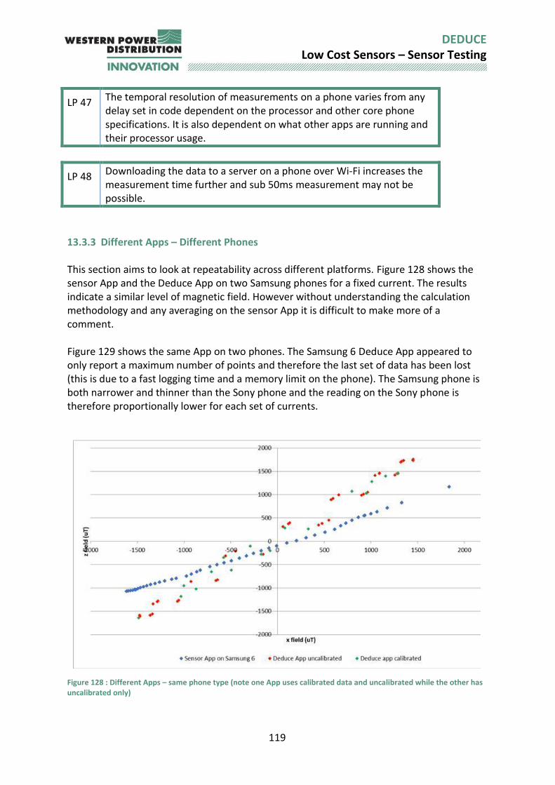
119
DEDUCE Low Cost Sensors – Sensor Testing
LP 47 The temporal resolution of measurements on a phone varies from any delay set in code dependent on the processor and other core phone specifications. It is also dependent on what other apps are running and their processor usage.
LP 48 Downloading the data to a server on a phone over Wi-Fi increases the measurement time further and sub 50ms measurement may not be possible.
13.3.3 Different Apps – Different Phones This section aims to look at repeatability across different platforms. Figure 128 shows the sensor App and the Deduce App on two Samsung phones for a fixed current. The results indicate a similar level of magnetic field. However without understanding the calculation methodology and any averaging on the sensor App it is difficult to make more of a comment. Figure 129 shows the same App on two phones. The Samsung 6 Deduce App appeared to only report a maximum number of points and therefore the last set of data has been lost (this is due to a fast logging time and a memory limit on the phone). The Samsung phone is both narrower and thinner than the Sony phone and the reading on the Sony phone is therefore proportionally lower for each set of currents.
Figure 128 : Different Apps – same phone type (note one App uses calibrated data and uncalibrated while the other has uncalibrated only)
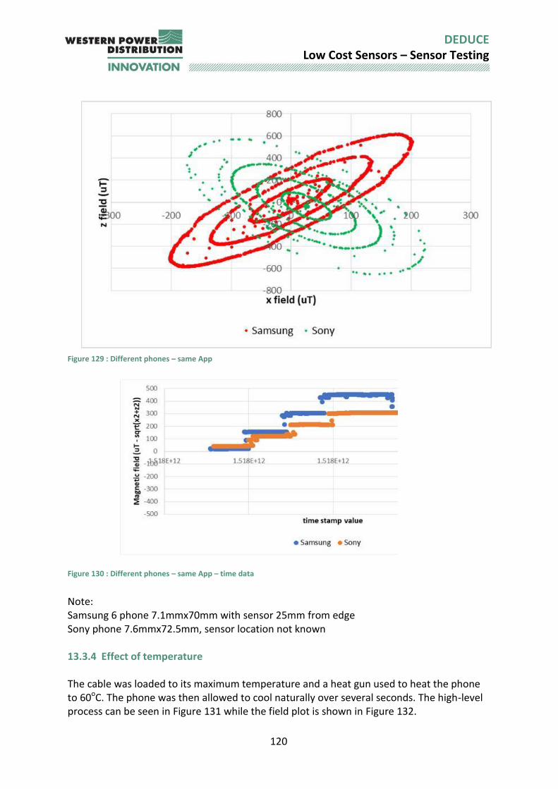
120
DEDUCE Low Cost Sensors – Sensor Testing
Figure 129 : Different phones – same App
Figure 130 : Different phones – same App – time data
Note: Samsung 6 phone 7.1mmx70mm with sensor 25mm from edge Sony phone 7.6mmx72.5mm, sensor location not known 13.3.4 Effect of temperature The cable was loaded to its maximum temperature and a heat gun used to heat the phone to 60oC. The phone was then allowed to cool naturally over several seconds. The high-level process can be seen in Figure 131 while the field plot is shown in Figure 132.
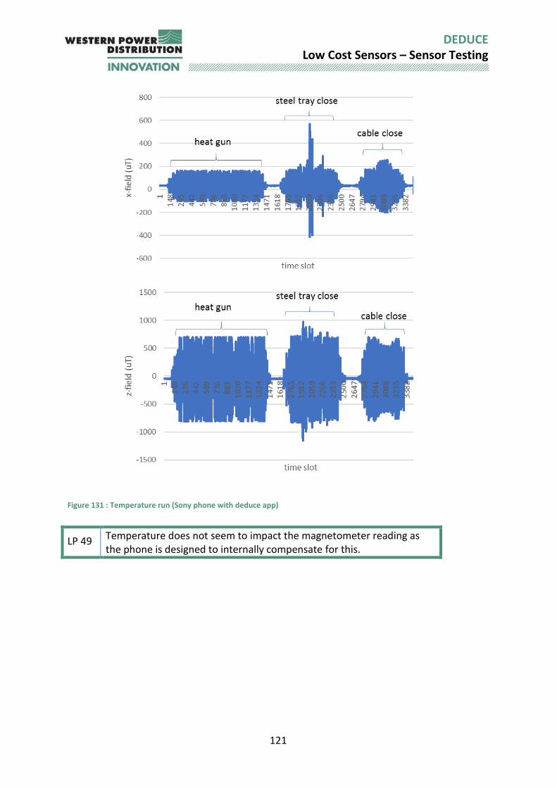
121
DEDUCE Low Cost Sensors – Sensor Testing
Figure 131 : Temperature run (Sony phone with deduce app)
LP 49 Temperature does not seem to impact the magnetometer reading as the phone is designed to internally compensate for this.
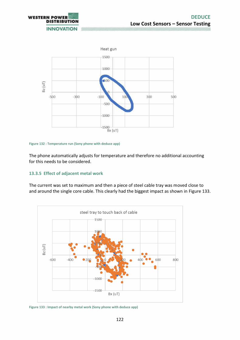
122
DEDUCE Low Cost Sensors – Sensor Testing
Figure 132 : Temperature run (Sony phone with deduce app)
The phone automatically adjusts for temperature and therefore no additional accounting for this needs to be considered. 13.3.5 Effect of adjacent metal work The current was set to maximum and then a piece of steel cable tray was moved close to and around the single core cable. This clearly had the biggest impact as shown in Figure 133.
Figure 133 : Impact of nearby metal work (Sony phone with deduce app)
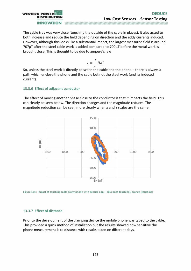
123
DEDUCE Low Cost Sensors – Sensor Testing
The cable tray was very close (touching the outside of the cable in places). It also acted to both increase and reduce the field depending on direction and the eddy currents induced. However, although this looks like a substantial impact, the largest measured field is around 707μT after the steel cable work is added compared to 700μT before the metal work is brought close. This is thought to be due to ampere’s law
𝐼 = ∫ 𝐻𝑑𝑙
So, unless the steel work is directly between the cable and the phone – there is always a path which enclose the phone and the cable but not the steel work (and its induced current). 13.3.6 Effect of adjacent conductor The effect of moving another phase close to the conductor is that it impacts the field. This can clearly be seen below. The direction changes and the magnitude reduces. The magnitude reduction can be seen more clearly when x and z scales are the same.
Figure 134 : Impact of touching cable (Sony phone with deduce app) – blue (not touching), orange (touching)
13.3.7 Effect of distance Prior to the development of the clamping device the mobile phone was taped to the cable. This provided a quick method of installation but the results showed how sensitive the phone measurement is to distance with results taken on different days.
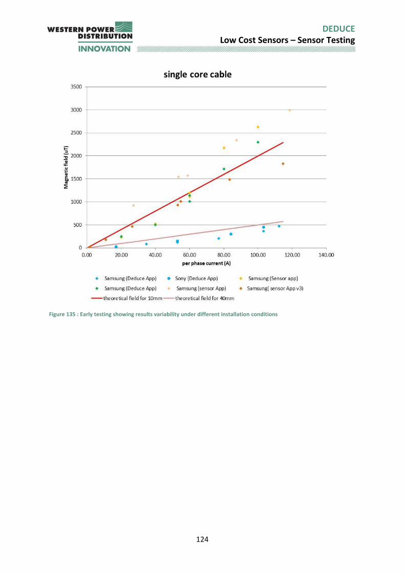
124
DEDUCE Low Cost Sensors – Sensor Testing
Figure 135 : Early testing showing results variability under different installation conditions
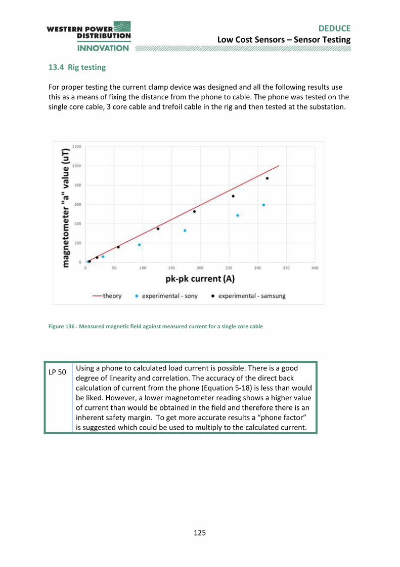
125
DEDUCE Low Cost Sensors – Sensor Testing
13.4 Rig testing For proper testing the current clamp device was designed and all the following results use this as a means of fixing the distance from the phone to cable. The phone was tested on the single core cable, 3 core cable and trefoil cable in the rig and then tested at the substation.
Figure 136 : Measured magnetic field against measured current for a single core cable
LP 50 Using a phone to calculated load current is possible. There is a good degree of linearity and correlation. The accuracy of the direct back calculation of current from the phone (Equation 5-18) is less than would be liked. However, a lower magnetometer reading shows a higher value of current than would be obtained in the field and therefore there is an inherent safety margin. To get more accurate results a “phone factor” is suggested which could be used to multiply to the calculated current.
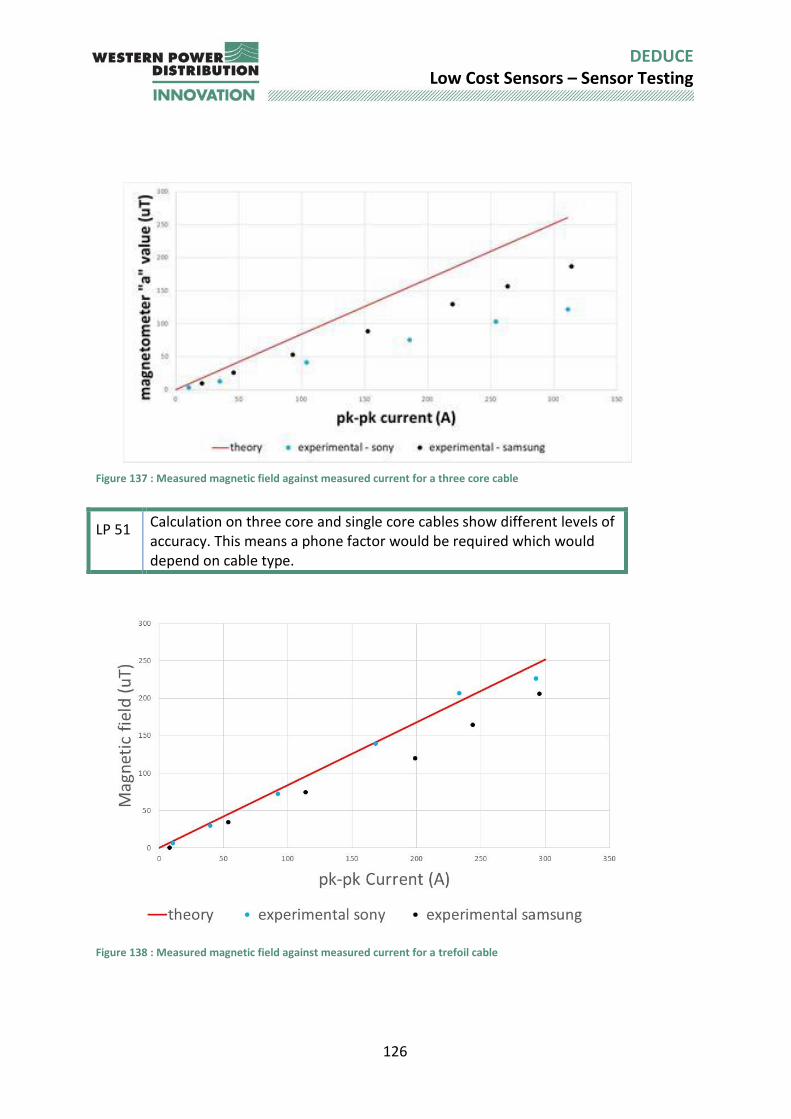
126
DEDUCE Low Cost Sensors – Sensor Testing
Figure 137 : Measured magnetic field against measured current for a three core cable
LP 51 Calculation on three core and single core cables show different levels of accuracy. This means a phone factor would be required which would depend on cable type.
Figure 138 : Measured magnetic field against measured current for a trefoil cable
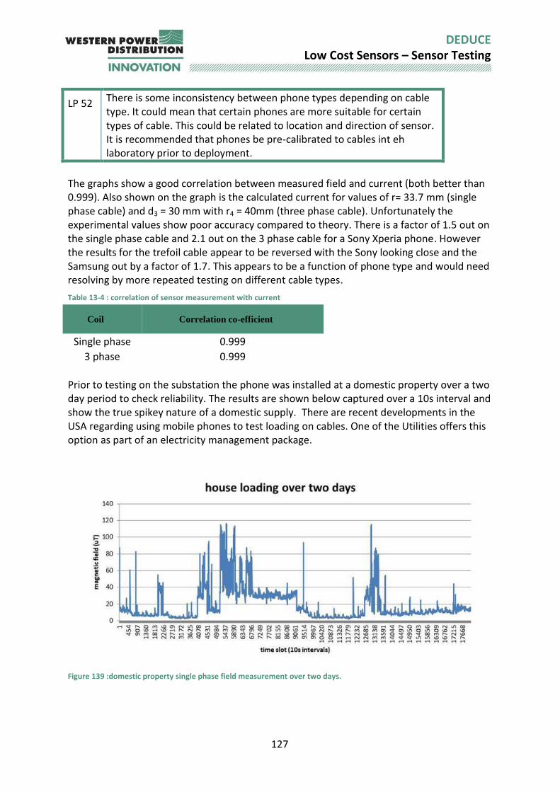
127
DEDUCE Low Cost Sensors – Sensor Testing
LP 52 There is some inconsistency between phone types depending on cable type. It could mean that certain phones are more suitable for certain types of cable. This could be related to location and direction of sensor. It is recommended that phones be pre-calibrated to cables int eh laboratory prior to deployment.
The graphs show a good correlation between measured field and current (both better than 0.999). Also shown on the graph is the calculated current for values of r= 33.7 mm (single phase cable) and d3 = 30 mm with r4 = 40mm (three phase cable). Unfortunately the experimental values show poor accuracy compared to theory. There is a factor of 1.5 out on the single phase cable and 2.1 out on the 3 phase cable for a Sony Xperia phone. However the results for the trefoil cable appear to be reversed with the Sony looking close and the Samsung out by a factor of 1.7. This appears to be a function of phone type and would need resolving by more repeated testing on different cable types.
Table 13-4 : correlation of sensor measurement with current
Coil Correlation co-efficient
Single phase 0.999
3 phase 0.999
Prior to testing on the substation the phone was installed at a domestic property over a two day period to check reliability. The results are shown below captured over a 10s interval and show the true spikey nature of a domestic supply. There are recent developments in the USA regarding using mobile phones to test loading on cables. One of the Utilities offers this option as part of an electricity management package.
Figure 139 :domestic property single phase field measurement over two days.
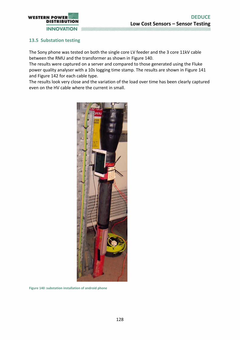
128
DEDUCE Low Cost Sensors – Sensor Testing
13.5 Substation testing The Sony phone was tested on both the single core LV feeder and the 3 core 11kV cable between the RMU and the transformer as shown in Figure 140. The results were captured on a server and compared to those generated using the Fluke power quality analyser with a 10s logging time stamp. The results are shown in Figure 141 and Figure 142 for each cable type. The results look very close and the variation of the load over time has been clearly captured even on the HV cable where the current in small.
Figure 140 :substation installation of android phone
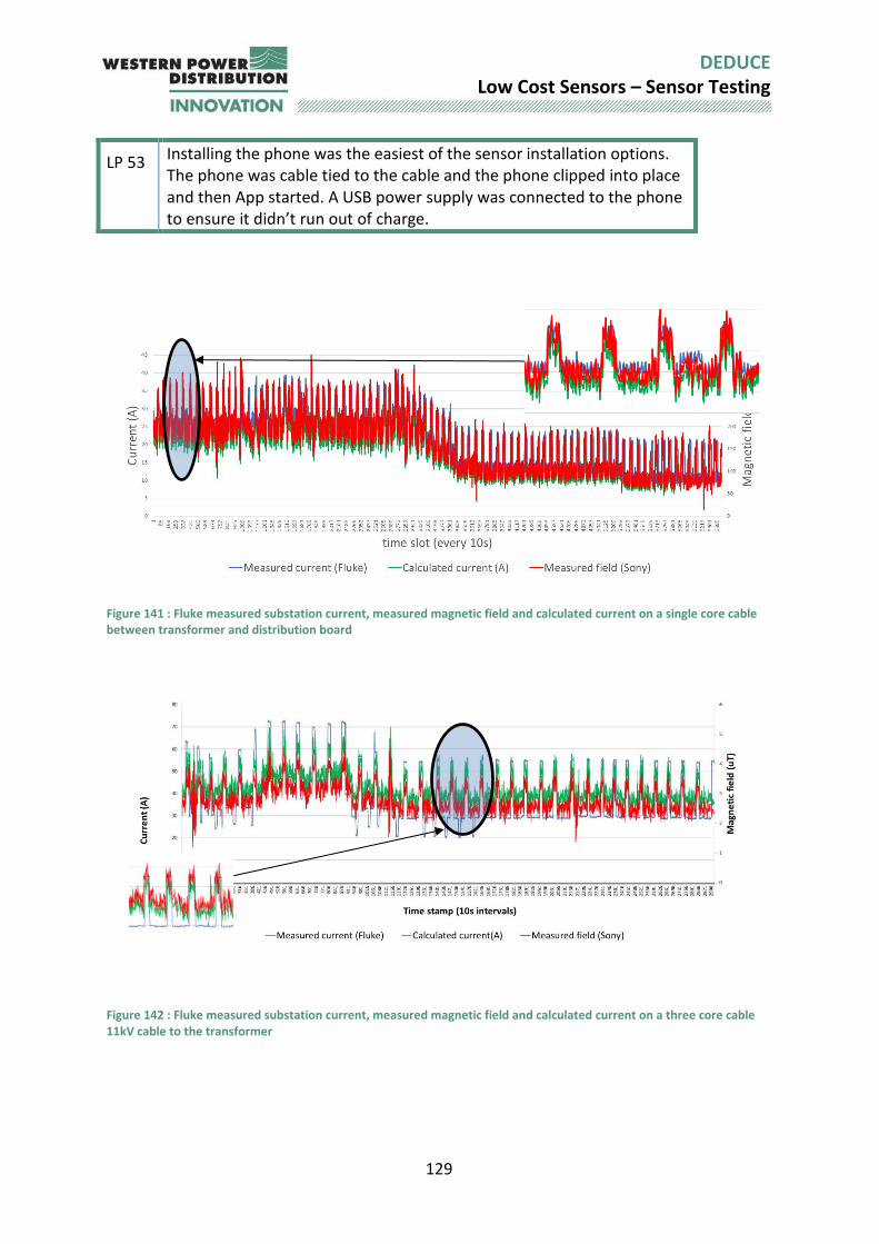
129
DEDUCE Low Cost Sensors – Sensor Testing
LP 53 Installing the phone was the easiest of the sensor installation options. The phone was cable tied to the cable and the phone clipped into place and then App started. A USB power supply was connected to the phone to ensure it didn’t run out of charge.
Figure 141 : Fluke measured substation current, measured magnetic field and calculated current on a single core cable between transformer and distribution board
Figure 142 : Fluke measured substation current, measured magnetic field and calculated current on a three core cable 11kV cable to the transformer
130
DEDUCE Low Cost Sensors – Sensor Testing
LP 54 A mobile phone magnetometer was successfully used to log data at a substation on both the LV and HV cable and the data was sent via WI-Fi to a server.
13.6 Summary A magnetometer is a promising candidate for long scale testing. However, the issue of distance of sensor from cable along with subsequent comparison to theory will enable knowledge of pre-calibration pre-deployment vs deployment calibration to be considered.
Comment
Application Can be used
to provide data from close to real time for DNR (several seconds) helping with fault restoration although not directional
exception reporting
load profiling
MDI The magnetometer part of the phone can provide a single phase or three phase estimate of current
Data Location Can be sent
Locally but only in small quantities as limited by phone memory
Server – to be accessed by anyone in the company
Data fidelity Time spans can be set to
Near real time (<15s)
10min intervals and above The data can be time stamped but isn’t synchronous
Data backup Very small local backup with link to server
Data form The data can be in the following form
Time stamped in any relevant format eg Peak/RMS over different time intervals where RMS is peak/root (2)
Failure mode Fail dead
Test Comments
Linearity Linear up to saturation but mathematical post-processing can be used to derive not saturated values
Effect of adjacent steel work
Substantial impact on field direction (both positive and negative). However, indication is that net field remains similar to that measured without steel. Therefore, this may not be an issue – further investigation is needed.
Effect of adjacent conductors
<10cm away some impact. Very close nearby cables (touching) in this instance reduces the field and therefore the measurement by approx. 20%
131
DEDUCE Low Cost Sensors – Sensor Testing
Effect of temperature
No obvious impact
Stability/reliability Appears stable
Ease of deployment Very straightforward, two cable ties onto a fixture to clip phone in place and addition of a power lead
Calibration Pre-lab based calibration appears to be an option rather than on-site calibration. It may be that some phone types don’t require this.
Time constants Delay of around >10ms for raw data and suggested 10s for average data to help remove issues with anti-aliasing
Accuracy 7.5% - However very sensitive to distance of sensor – so proper fixture required
Correlation to loading
0.999
Sensitivity Mostly to distance and adjacent conductors.
Repeatability Repeatable over different phones and with different Apps
Data Storage Data can be stored (for small time periods) at 10ms intervals or uploaded to a server in 50ms intervals. Post processing of data will add to this.
Other factors Comments
Primary sensing element
Magnetometer
Power/excitation Phone charging cable connected to 230V needed
Amplification Not needed and in fact distance increases may be used to desensitise
Analogue filtering Not required
Data conversion Maybe done on phone
Digital information processing
Elliptical curve fitting process required to capture data
Digital communication processing
Method proven at simple level with time stamp and auto- download to a server based on location. Additional setup procedures need to be sorted.
Communication Mobile network
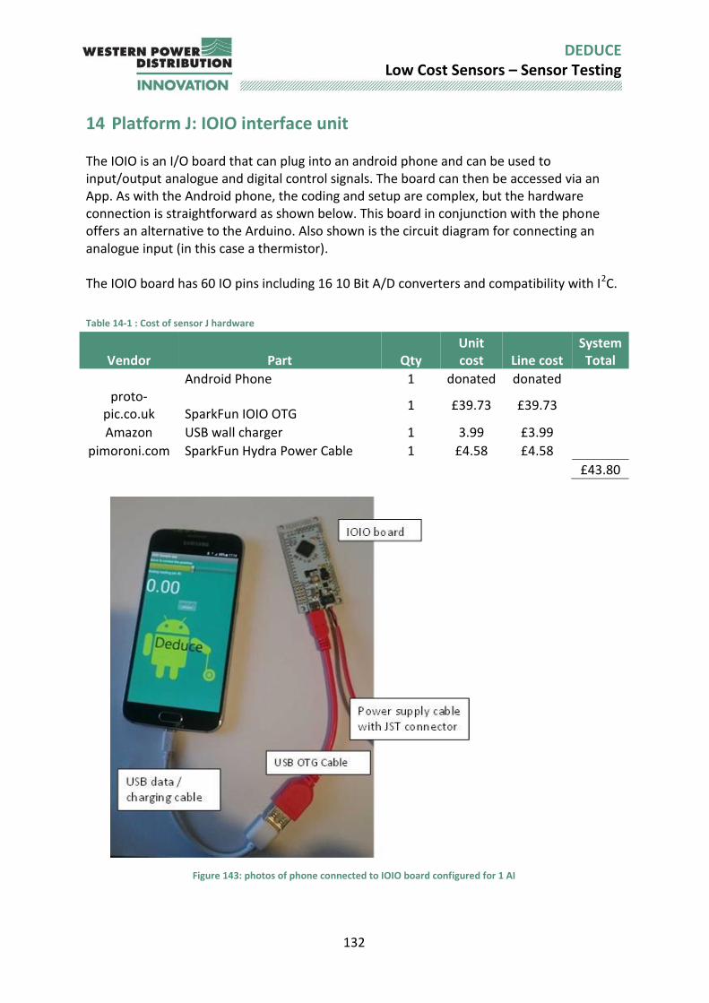
132
DEDUCE Low Cost Sensors – Sensor Testing
14 Platform J: IOIO interface unit The IOIO is an I/O board that can plug into an android phone and can be used to input/output analogue and digital control signals. The board can then be accessed via an App. As with the Android phone, the coding and setup are complex, but the hardware connection is straightforward as shown below. This board in conjunction with the phone offers an alternative to the Arduino. Also shown is the circuit diagram for connecting an analogue input (in this case a thermistor). The IOIO board has 60 IO pins including 16 10 Bit A/D converters and compatibility with I2C.
Table 14-1 : Cost of sensor J hardware
Vendor Part Qty Unit cost Line cost
System Total
Android Phone 1 donated donated
proto-pic.co.uk SparkFun IOIO OTG
1 £39.73 £39.73
Amazon USB wall charger 1 3.99 £3.99 pimoroni.com SparkFun Hydra Power Cable 1 £4.58 £4.58 £43.80
Figure 143: photos of phone connected to IOIO board configured for 1 AI
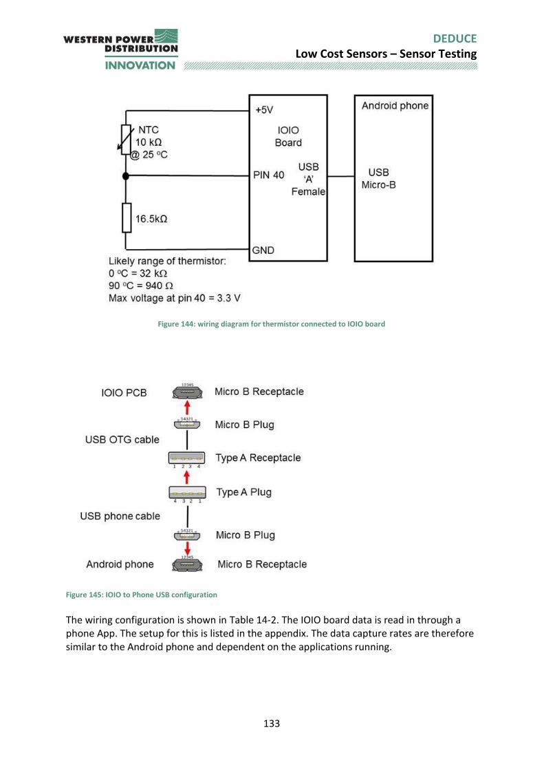
133
DEDUCE Low Cost Sensors – Sensor Testing
Figure 144: wiring diagram for thermistor connected to IOIO board
Figure 145: IOIO to Phone USB configuration
The wiring configuration is shown in Table 14-2. The IOIO board data is read in through a phone App. The setup for this is listed in the appendix. The data capture rates are therefore similar to the Android phone and dependent on the applications running.
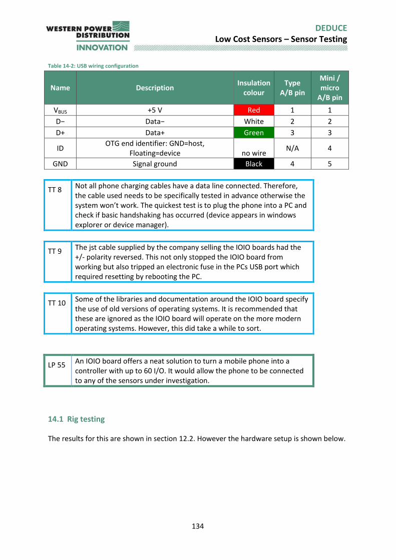
134
DEDUCE Low Cost Sensors – Sensor Testing
Table 14-2: USB wiring configuration
Name Description Insulation
colour Type
A/B pin
Mini / micro
A/B pin
VBUS +5 V Red 1 1
D− Data− White 2 2
D+ Data+ Green 3 3
ID OTG end identifier: GND=host,
Floating=device no wire N/A 4
GND Signal ground Black 4 5
TT 8 Not all phone charging cables have a data line connected. Therefore, the cable used needs to be specifically tested in advance otherwise the system won’t work. The quickest test is to plug the phone into a PC and check if basic handshaking has occurred (device appears in windows explorer or device manager).
TT 9 The jst cable supplied by the company selling the IOIO boards had the +/- polarity reversed. This not only stopped the IOIO board from working but also tripped an electronic fuse in the PCs USB port which required resetting by rebooting the PC.
TT 10 Some of the libraries and documentation around the IOIO board specify the use of old versions of operating systems. It is recommended that these are ignored as the IOIO board will operate on the more modern operating systems. However, this did take a while to sort.
LP 55 An IOIO board offers a neat solution to turn a mobile phone into a controller with up to 60 I/O. It would allow the phone to be connected to any of the sensors under investigation.
14.1 Rig testing The results for this are shown in section 12.2. However the hardware setup is shown below.
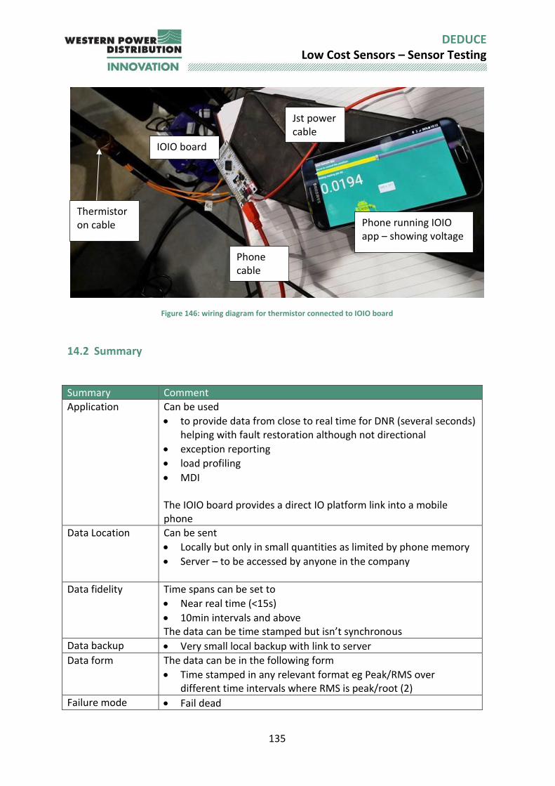
135
DEDUCE Low Cost Sensors – Sensor Testing
Figure 146: wiring diagram for thermistor connected to IOIO board
14.2 Summary
Summary Comment
Application Can be used
to provide data from close to real time for DNR (several seconds) helping with fault restoration although not directional
exception reporting
load profiling
MDI The IOIO board provides a direct IO platform link into a mobile phone
Data Location Can be sent
Locally but only in small quantities as limited by phone memory
Server – to be accessed by anyone in the company
Data fidelity Time spans can be set to
Near real time (<15s)
10min intervals and above The data can be time stamped but isn’t synchronous
Data backup Very small local backup with link to server
Data form The data can be in the following form
Time stamped in any relevant format eg Peak/RMS over different time intervals where RMS is peak/root (2)
Failure mode Fail dead
Thermistor on cable
Jst power cable
IOIO board
Phone running IOIO app – showing voltage
Phone cable
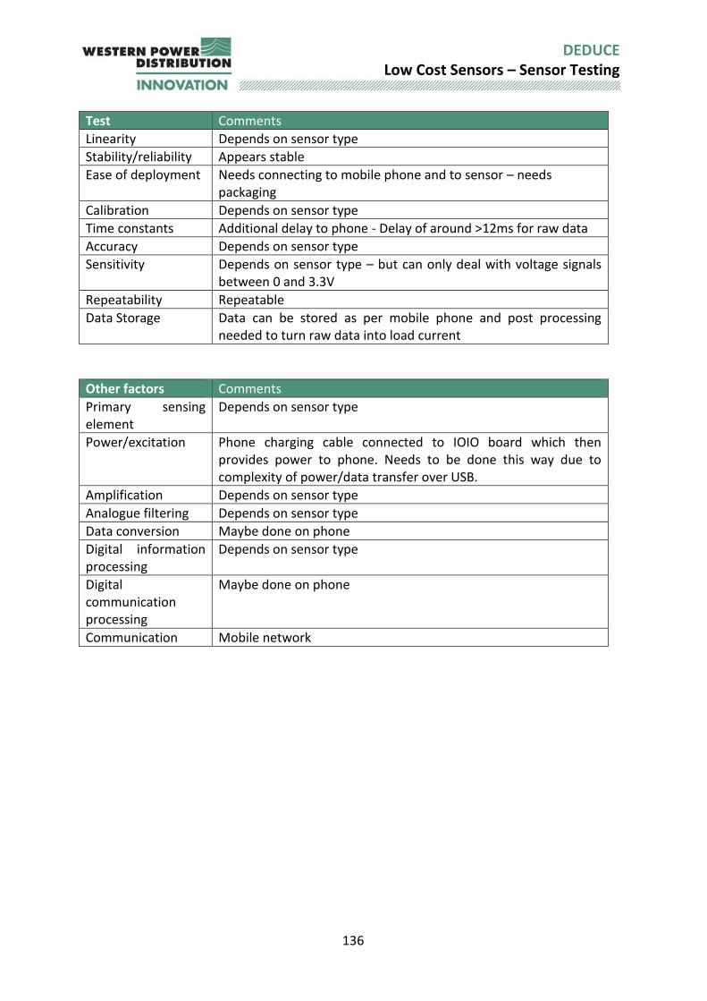
136
DEDUCE Low Cost Sensors – Sensor Testing
Test Comments
Linearity Depends on sensor type
Stability/reliability Appears stable
Ease of deployment Needs connecting to mobile phone and to sensor – needs packaging
Calibration Depends on sensor type
Time constants Additional delay to phone - Delay of around >12ms for raw data
Accuracy Depends on sensor type
Sensitivity Depends on sensor type – but can only deal with voltage signals between 0 and 3.3V
Repeatability Repeatable
Data Storage Data can be stored as per mobile phone and post processing needed to turn raw data into load current
Other factors Comments
Primary sensing element
Depends on sensor type
Power/excitation Phone charging cable connected to IOIO board which then provides power to phone. Needs to be done this way due to complexity of power/data transfer over USB.
Amplification Depends on sensor type
Analogue filtering Depends on sensor type
Data conversion Maybe done on phone
Digital information processing
Depends on sensor type
Digital communication processing
Maybe done on phone
Communication Mobile network
137
DEDUCE Low Cost Sensors – Sensor Testing
15 Platform K: Arduino The Arduino is a micro-controller device which can be used to read input signals and communicate with devices. The Arduino development system can be (and has been) used to read signals from both analogue and digital sensors, via voltage and I2C serial signals respectively. Initial Arduino development used the low-cost Arduino Uno board which is adequate to read signals and transmit them to PC as ASCII text via USB. Sending data via GPRS requires considerably more memory, so the LinkitOne PCB was used which also has on-board WIFI, GPRS, GPS capability and a real time clock which is important for accurate data timestamping.
Table 15-1 : Cost of sensor k hardware
Vendor Part Qty Unit cost Line cost
RS Arduino Uno 1 £14.99 £14.99
- or -
Rapid LinkitOne PCB (Arduino compatible) 1 £44.24 £44.24 The Arduino PCBS can be linked to built-in libraries are available for commonly used add-on boards such as MEMS sensors. For example, a program to read data and I2C MEMS sensor, calculate running averages and exponential averages and send data as ASCII text to USB port with a timestamp required only 120 lines of code including comments, variable definitions and spacing. It is important to note the limitations of what ‘Arduino compatible’ does mean
Rows of pins along outside edge of PCB standard pitch and physical pinouts
Common voltages used
Ability to upload code via built-in bootloader via USB avoiding the need for a separate programmer PCB as with off the shelf micro-controller chips
Use of a common C++ library called ‘Wiring’ for core functions which can be coded, compiled and uploaded from the Arduino IDE.
USB debug port sharing the same physical USB port used for code upload. However there are also many differences even within the Genuine Arduino/Genuino range of PCBs in addition to third party PCBS including:
Arduino libraries for third party devices such as sensor and communications boards may be compatible only with certain microcontrollers for example the Sparkfun MPU9250 library is compatible with the Arduino Uno and Mega but not the SEEED Studio LinkitOne.
Digital pins used for the same serial protocol may vary between different PCBs
Taking the Arduino Uno as the base case, other PCBs may have more analogue/digital channels and other serial and communication ports, for example the Mega has lots of extra analogue/digital pins. The LinkitOne has additional Grove ports and built in GSM/GPRS/Wifi/Bluetooth/GPS circuits.
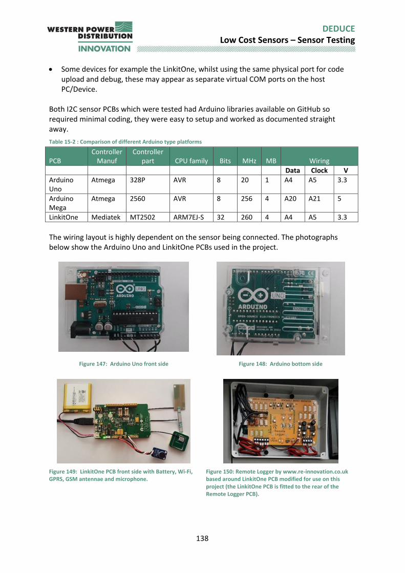
138
DEDUCE Low Cost Sensors – Sensor Testing
Some devices for example the LinkitOne, whilst using the same physical port for code upload and debug, these may appear as separate virtual COM ports on the host PC/Device.
Both I2C sensor PCBs which were tested had Arduino libraries available on GitHub so required minimal coding, they were easy to setup and worked as documented straight away.
Table 15-2 : Comparison of different Arduino type platforms
PCB Controller
Manuf Controller
part CPU family Bits MHz MB Wiring
Data Clock V
Arduino Uno
Atmega 328P AVR 8 20 1 A4 A5 3.3
Arduino Mega
Atmega 2560 AVR 8 256 4 A20 A21 5
LinkitOne Mediatek MT2502 ARM7EJ-S 32 260 4 A4 A5 3.3
The wiring layout is highly dependent on the sensor being connected. The photographs below show the Arduino Uno and LinkitOne PCBs used in the project.
Figure 147: Arduino Uno front side Figure 148: Arduino bottom side
Figure 149: LinkitOne PCB front side with Battery, Wi-Fi, GPRS, GSM antennae and microphone.
Figure 150: Remote Logger by www.re-innovation.co.uk based around LinkitOne PCB modified for use on this project (the LinkitOne PCB is fitted to the rear of the Remote Logger PCB).
139
DEDUCE Low Cost Sensors – Sensor Testing
15.1 Settings and software The Arduino settings and source code used are shown in Appendix 20
15.2 GSM/GPRS PCBs Both GSM/GPRS communications PCBs come in shield format so were easy to connect and had Arduino libraries available. However the DFRobot setup was convoluted requiring multiple user interventions to reboot/upload/switch to debug operation. The manual was vague and it was not possible to even prove the fundamental communication between the Arduino and the Comms board let alone send an SMS. Sending an SMS is the simplest test for a GSM/GPRS comms board as SMS sending requires only an in-credit SIM card without the APN setup required for GPRS data communications.
Table 15-3 : Comparison of different Arduino GPRS platforms
Compatibility
Manufacturer Model Band GiffGaff PP
Vodafone PP data
only
Seeedstudio / Mediatek
LinkitOne 2G
Adafruit Fona SIM808 Shield
2G
Table 15-4 : GPRS setup for Adafruit Fona SIM808 shield
Adafruit Fona SIM808 Function
Default Arduino PIN
Rx 2
Tx 3
RST 4
RTS 5
RI NC
Net NC
Pwr NC
Key GND
DTR NC
15.3 Rig testing Two types of ‘9 axis’ movement PCBs were tested the Adafruit LSM9DS0 and the SparkFun MPU-9250. Two types of PCB were tested the Arduino Uno and the LinkitOne. The sensors and controllers were compared for measurement timing. No delays were set in the program, so data would be saved as fast as the sensor and controller allowed. No averaging or calculations were conducted on the raw data it was simply read from the sensor and written to the USB serial port. The MPU-9250 sample rate was set to the highest possible
140
DEDUCE Low Cost Sensors – Sensor Testing
which was 100Hz. The shortest measurement interval was with the MPU_9250 connected to the LinkitOne with 3 channels measured which averaged 31 seconds per measurement. The slowest was with the LSM9DS0 connected to the Arduino Uno with 9 channels measured which averaged 78s per measurement.
Table 15-5 : Sensor data capture rates using the serial link
Controller
Sensor
Data channels recorded Measurement interval [sec]
Mag Accel Analogue Total Min Mean Max Range Arduino Uno MPU_9250
3 0 0 3 22 43 46 24
Arduino Uno MPU_9250
3 3 3 9 42 56 59 17
Arduino Uno LSM9DS0
3 0 0 3 25 37 38 13
Arduino Uno LSM9DS0
3 3 3 9 62 78 81 19
Linkit One MPU_9250 3 0 0 3 9 31 50 41 Linkit One MPU_9250 3 3 3 9 14 40 61 47 Linkit One LSM9DS0 Library not compatible
Linkit One LSM9DS0 Library not compatible
15.3.1 Calibration of A-D It was noted that the analogue inputs float by up to 0.5V if nothing is connected to any of the terminals. If some terminals are left unconnected they tend to show the value from adjacent terminals. This is common even in high quality analogue dataloggers where adjacent channels are often time domain multiplexed into a single high precision analogue-digital circuit.
TT 11 It is wise to connect jumpers from unused analogue input terminals to ground to prevent misunderstandings in the measurements.
The scaling factor for DC voltage to reported reading was confirmed to be 205 +/-0.5%.
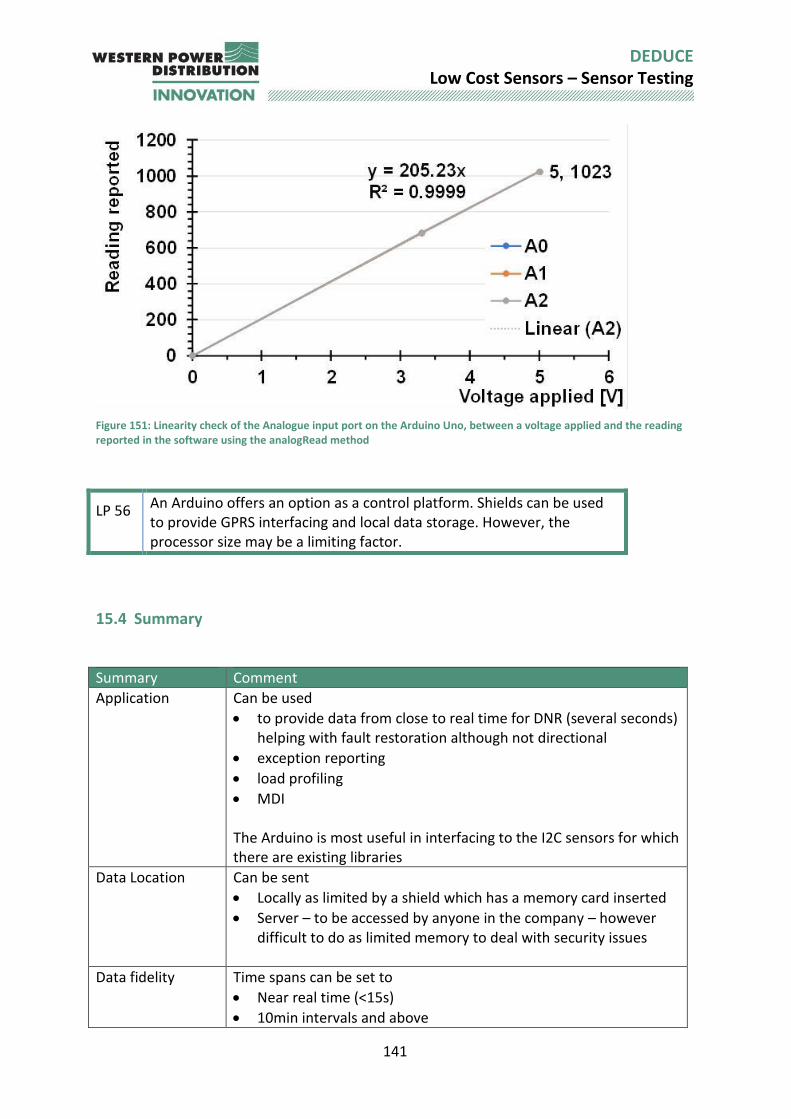
141
DEDUCE Low Cost Sensors – Sensor Testing
Figure 151: Linearity check of the Analogue input port on the Arduino Uno, between a voltage applied and the reading reported in the software using the analogRead method
LP 56 An Arduino offers an option as a control platform. Shields can be used to provide GPRS interfacing and local data storage. However, the processor size may be a limiting factor.
15.4 Summary
Summary Comment
Application Can be used
to provide data from close to real time for DNR (several seconds) helping with fault restoration although not directional
exception reporting
load profiling
MDI The Arduino is most useful in interfacing to the I2C sensors for which there are existing libraries
Data Location Can be sent
Locally as limited by a shield which has a memory card inserted
Server – to be accessed by anyone in the company – however difficult to do as limited memory to deal with security issues
Data fidelity Time spans can be set to
Near real time (<15s)
10min intervals and above
142
DEDUCE Low Cost Sensors – Sensor Testing
The data can be time stamped but isn’t synchronous
Data backup Only through addition of external shield
Data form The data can be in the following form
Time stamped in any relevant format eg Peak/RMS over different time intervals where RMS is peak/root (2)
Failure mode Fail dead
Test Comments
Linearity Depends on sensor type
Stability/reliability Appears stable
Ease of deployment Needs connecting to mobile phone and to sensor – needs packaging
Calibration Depends on sensor type
Time constants Additional delay to phone - Delay of around >12ms for raw data
Accuracy Depends on sensor type
Sensitivity Depends on sensor type – but can only deal with voltage signals between 0 and 3.3V and up to 16 bits which needs careful planning as it doesn’t deal nicely with floating point numbers
Repeatability Repeatable
Data Storage Only through addition of external shield and post processing needed to turn raw data into load current
Other factors Comments
Primary sensing element
Depends on sensor type
Power/excitation Phone charging usb cable connected to arduino board which then provides power to I2C devices
Amplification Depends on sensor type
Analogue filtering Depends on sensor type
Data conversion Maybe done on arduino
Digital information processing
Depends on sensor type
Digital communication processing
Maybe done on Arduino but limited by memory
Communication Mobile network through additional shield board
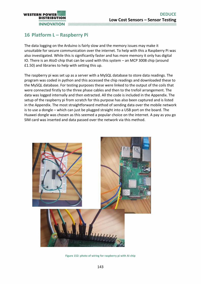
143
DEDUCE Low Cost Sensors – Sensor Testing
16 Platform L – Raspberry Pi The data logging on the Arduino is fairly slow and the memory issues may make it unsuitable for secure communication over the internet. To help with this a Raspberry Pi was also investigated. While this is significantly faster and has more memory it only has digital IO. There is an AtoD chip that can be used with this system – an MCP 3008 chip (around £1.50) and libraries to help with setting this up. The raspberry pi was set up as a server with a MySQL database to store data readings. The program was coded in python and this accessed the chip readings and downloaded these to the MySQL database. For testing purposes these were linked to the output of the coils that were connected firstly to the three phase cables and then to the trefoil arrangement. The data was logged internally and then extracted. All the code is included in the Appendix. The setup of the raspberry pi from scratch for this purpose has also been captured and is listed in the Appendix. The most straightforward method of sending data over the mobile network is to use a dongle – which can just be plugged straight into a USB port on the board. The Huawei dongle was chosen as this seemed a popular choice on the internet. A pay as you go SIM card was inserted and data passed over the network via this method.
Figure 152: photo of wiring for raspberry pi with AI chip
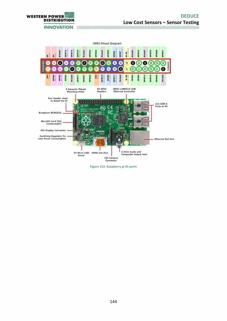
144
DEDUCE Low Cost Sensors – Sensor Testing
Figure 153: Raspberry pi IO ports
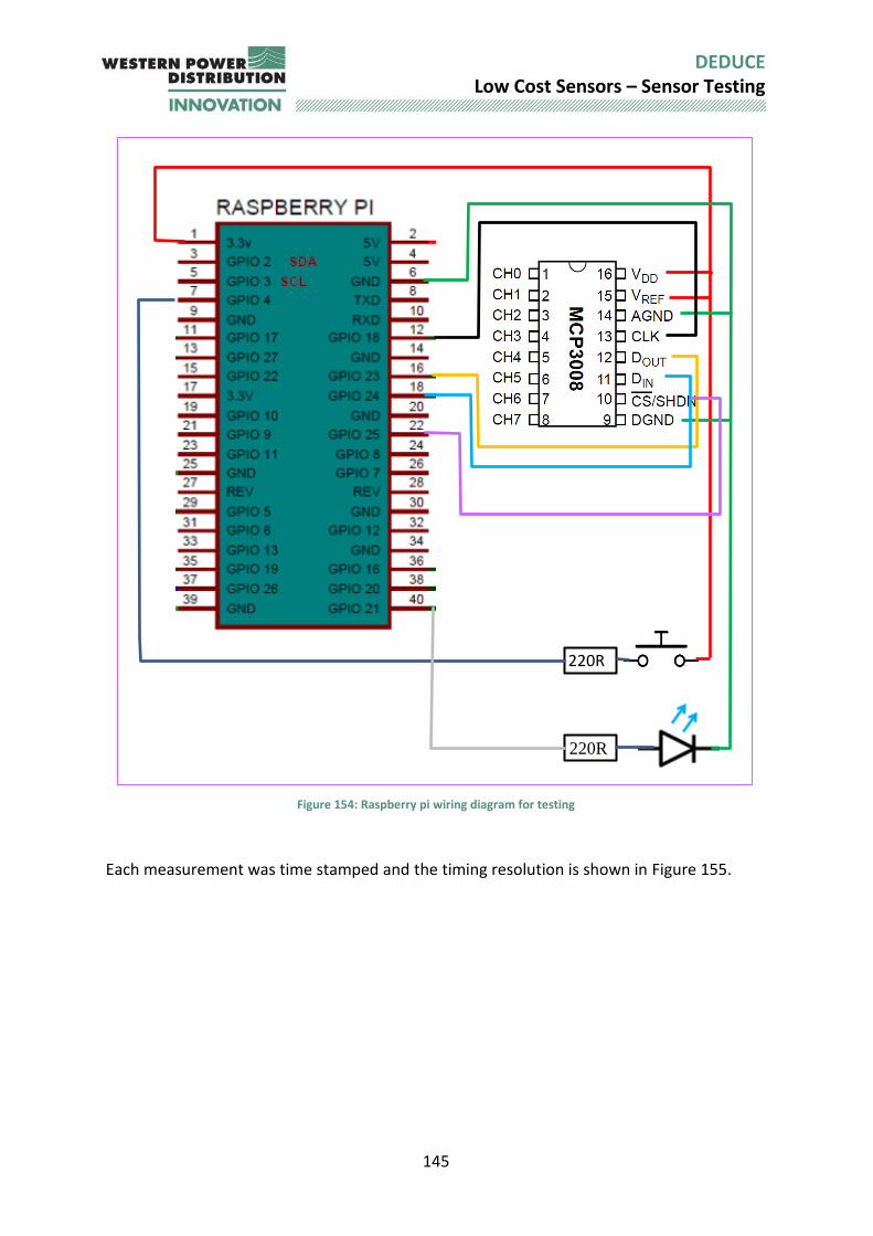
145
DEDUCE Low Cost Sensors – Sensor Testing
Figure 154: Raspberry pi wiring diagram for testing
Each measurement was time stamped and the timing resolution is shown in Figure 155.
220R
220R
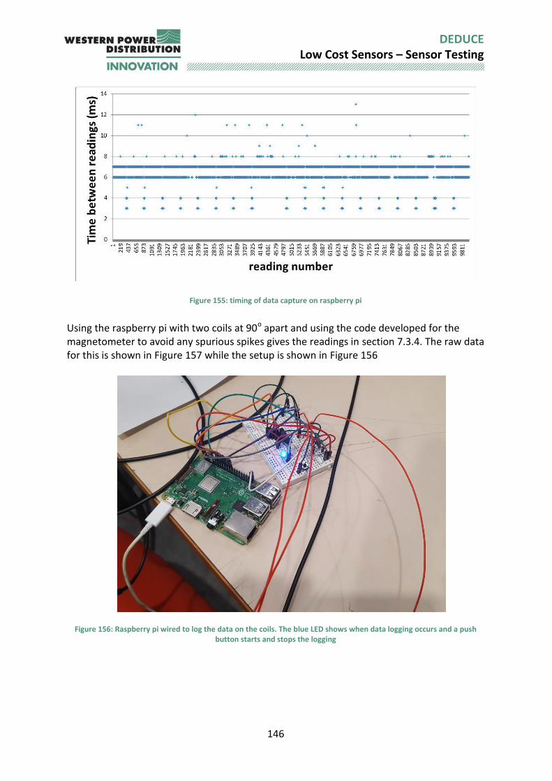
146
DEDUCE Low Cost Sensors – Sensor Testing
Figure 155: timing of data capture on raspberry pi
Using the raspberry pi with two coils at 90o apart and using the code developed for the magnetometer to avoid any spurious spikes gives the readings in section 7.3.4. The raw data for this is shown in Figure 157 while the setup is shown in Figure 156
Figure 156: Raspberry pi wired to log the data on the coils. The blue LED shows when data logging occurs and a push
button starts and stops the logging
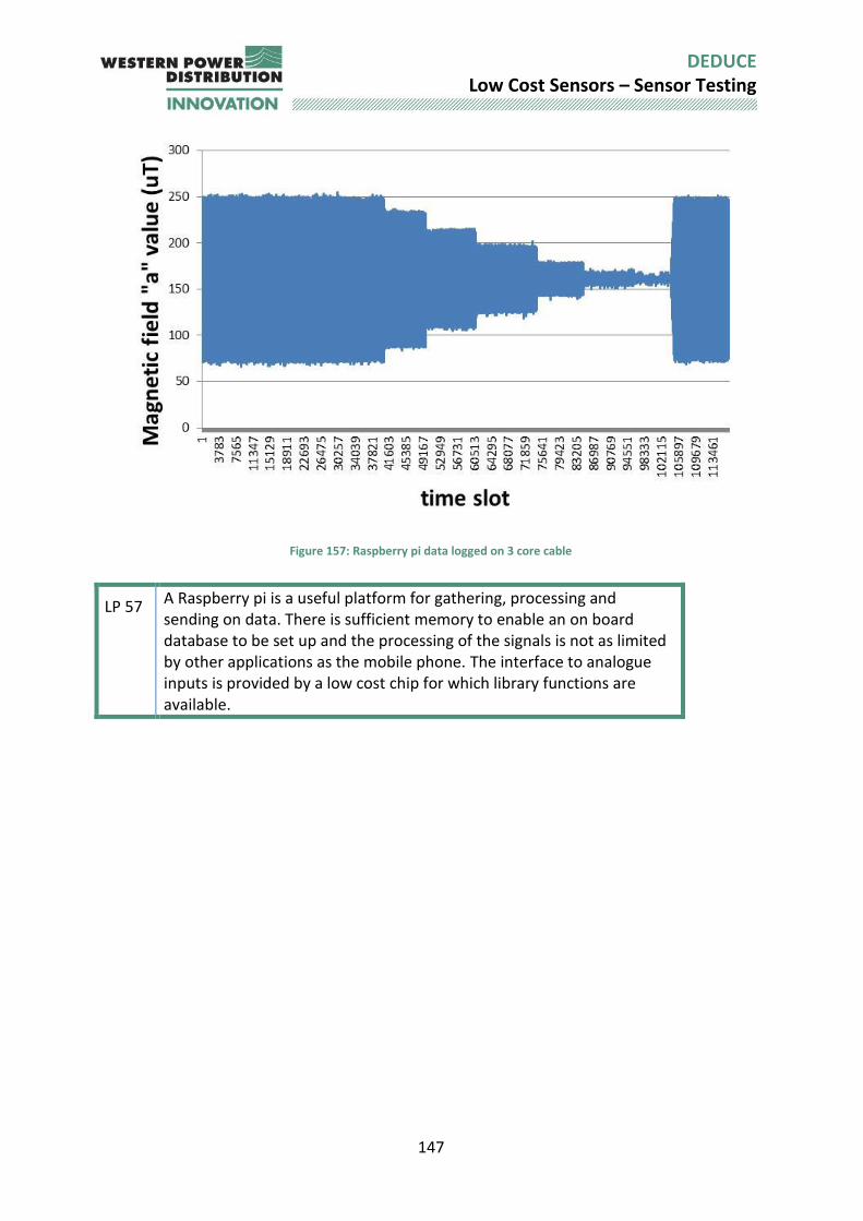
147
DEDUCE Low Cost Sensors – Sensor Testing
Figure 157: Raspberry pi data logged on 3 core cable
LP 57 A Raspberry pi is a useful platform for gathering, processing and sending on data. There is sufficient memory to enable an on board database to be set up and the processing of the signals is not as limited by other applications as the mobile phone. The interface to analogue inputs is provided by a low cost chip for which library functions are available.
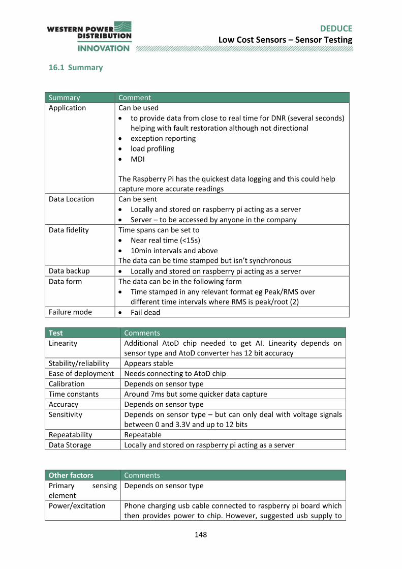
148
DEDUCE Low Cost Sensors – Sensor Testing
16.1 Summary
Summary Comment
Application Can be used
to provide data from close to real time for DNR (several seconds) helping with fault restoration although not directional
exception reporting
load profiling
MDI The Raspberry Pi has the quickest data logging and this could help capture more accurate readings
Data Location Can be sent
Locally and stored on raspberry pi acting as a server
Server – to be accessed by anyone in the company
Data fidelity Time spans can be set to
Near real time (<15s)
10min intervals and above The data can be time stamped but isn’t synchronous
Data backup Locally and stored on raspberry pi acting as a server
Data form The data can be in the following form
Time stamped in any relevant format eg Peak/RMS over different time intervals where RMS is peak/root (2)
Failure mode Fail dead
Test Comments
Linearity Additional AtoD chip needed to get AI. Linearity depends on sensor type and AtoD converter has 12 bit accuracy
Stability/reliability Appears stable
Ease of deployment Needs connecting to AtoD chip
Calibration Depends on sensor type
Time constants Around 7ms but some quicker data capture
Accuracy Depends on sensor type
Sensitivity Depends on sensor type – but can only deal with voltage signals between 0 and 3.3V and up to 12 bits
Repeatability Repeatable
Data Storage Locally and stored on raspberry pi acting as a server
Other factors Comments
Primary sensing element
Depends on sensor type
Power/excitation Phone charging usb cable connected to raspberry pi board which then provides power to chip. However, suggested usb supply to
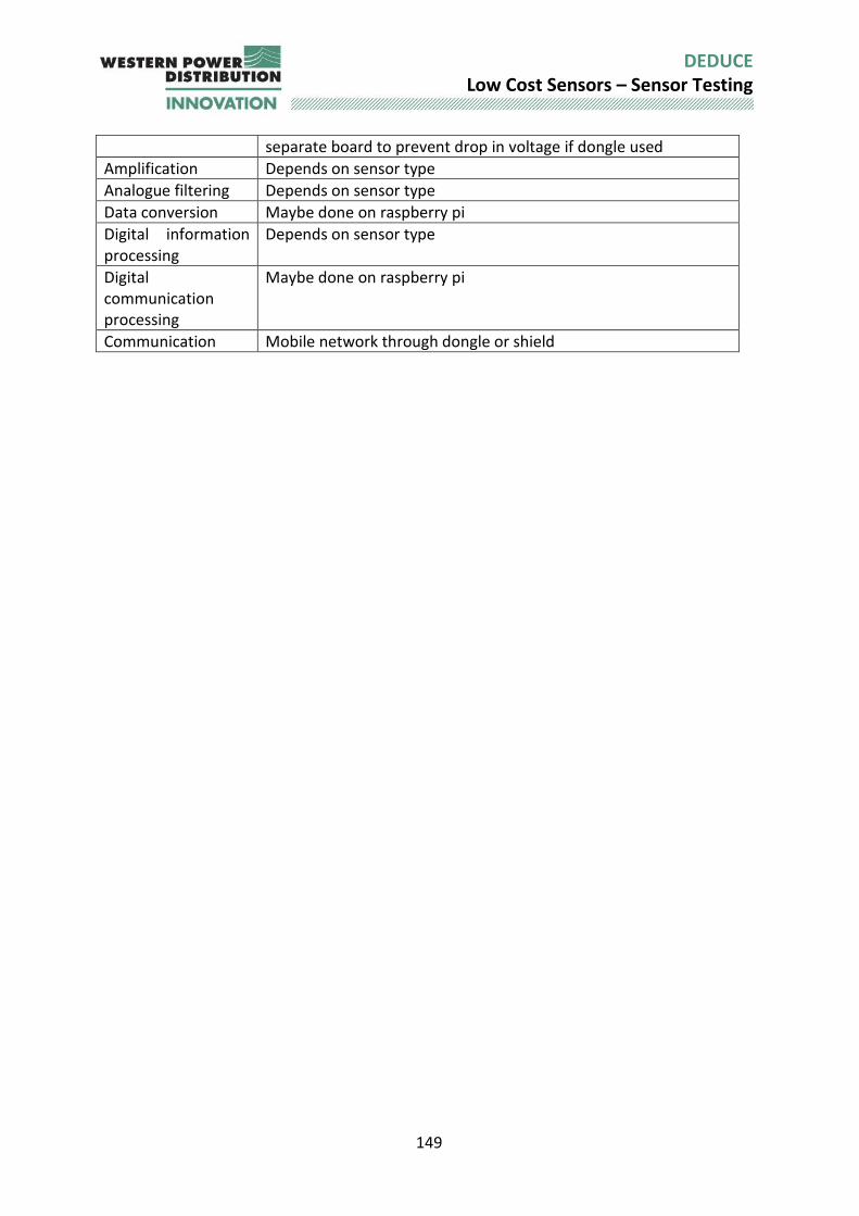
149
DEDUCE Low Cost Sensors – Sensor Testing
separate board to prevent drop in voltage if dongle used
Amplification Depends on sensor type
Analogue filtering Depends on sensor type
Data conversion Maybe done on raspberry pi
Digital information processing
Depends on sensor type
Digital communication processing
Maybe done on raspberry pi
Communication Mobile network through dongle or shield
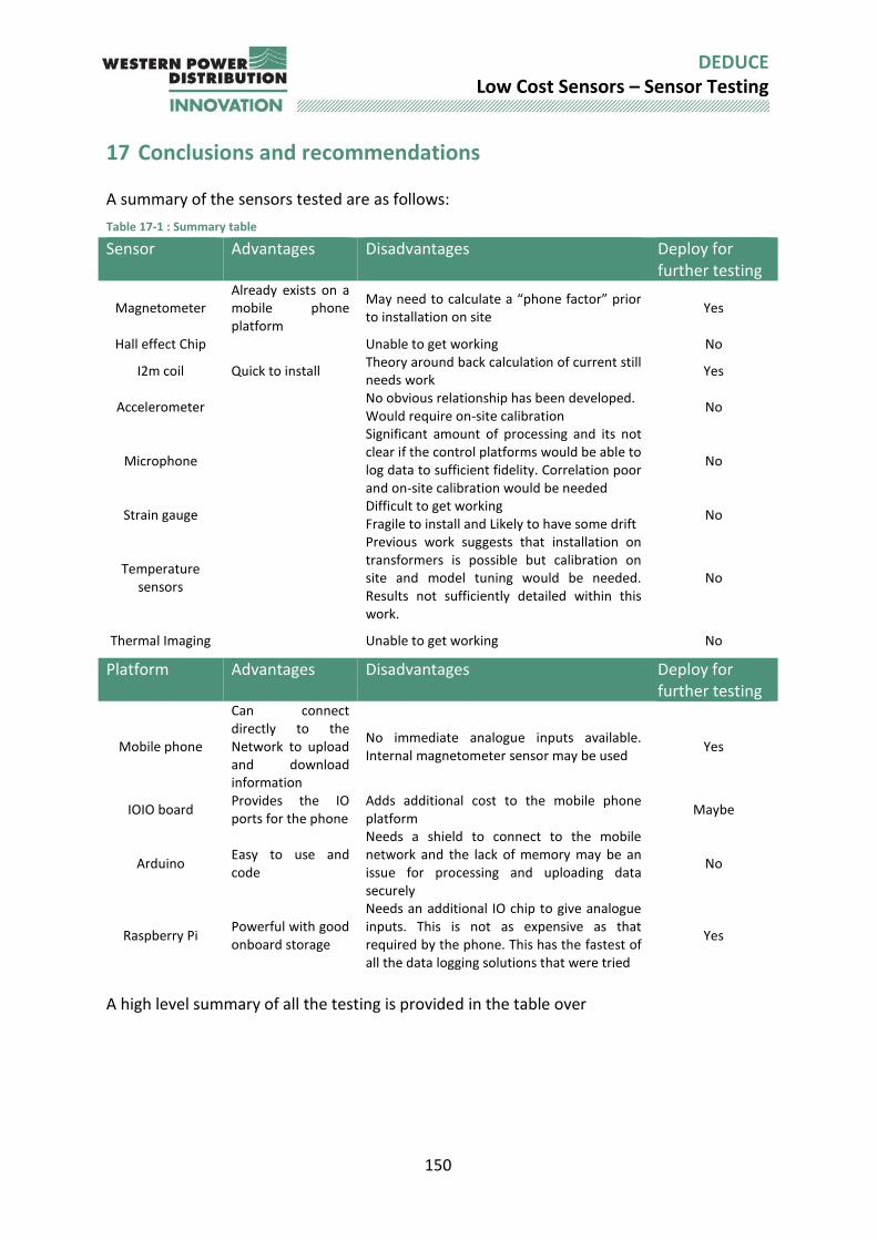
150
DEDUCE Low Cost Sensors – Sensor Testing
17 Conclusions and recommendations A summary of the sensors tested are as follows:
Table 17-1 : Summary table
Sensor Advantages Disadvantages Deploy for further testing
Magnetometer Already exists on a mobile phone platform
May need to calculate a “phone factor” prior to installation on site
Yes
Hall effect Chip Unable to get working No
I2m coil Quick to install Theory around back calculation of current still needs work
Yes
Accelerometer No obvious relationship has been developed. Would require on-site calibration
No
Microphone
Significant amount of processing and its not clear if the control platforms would be able to log data to sufficient fidelity. Correlation poor and on-site calibration would be needed
No
Strain gauge Difficult to get working Fragile to install and Likely to have some drift
No
Temperature sensors
Previous work suggests that installation on transformers is possible but calibration on site and model tuning would be needed. Results not sufficiently detailed within this work.
No
Thermal Imaging Unable to get working No
Platform Advantages Disadvantages Deploy for further testing
Mobile phone
Can connect directly to the Network to upload and download information
No immediate analogue inputs available. Internal magnetometer sensor may be used
Yes
IOIO board Provides the IO ports for the phone
Adds additional cost to the mobile phone platform
Maybe
Arduino Easy to use and code
Needs a shield to connect to the mobile network and the lack of memory may be an issue for processing and uploading data securely
No
Raspberry Pi Powerful with good onboard storage
Needs an additional IO chip to give analogue inputs. This is not as expensive as that required by the phone. This has the fastest of all the data logging solutions that were tried
Yes
A high level summary of all the testing is provided in the table over
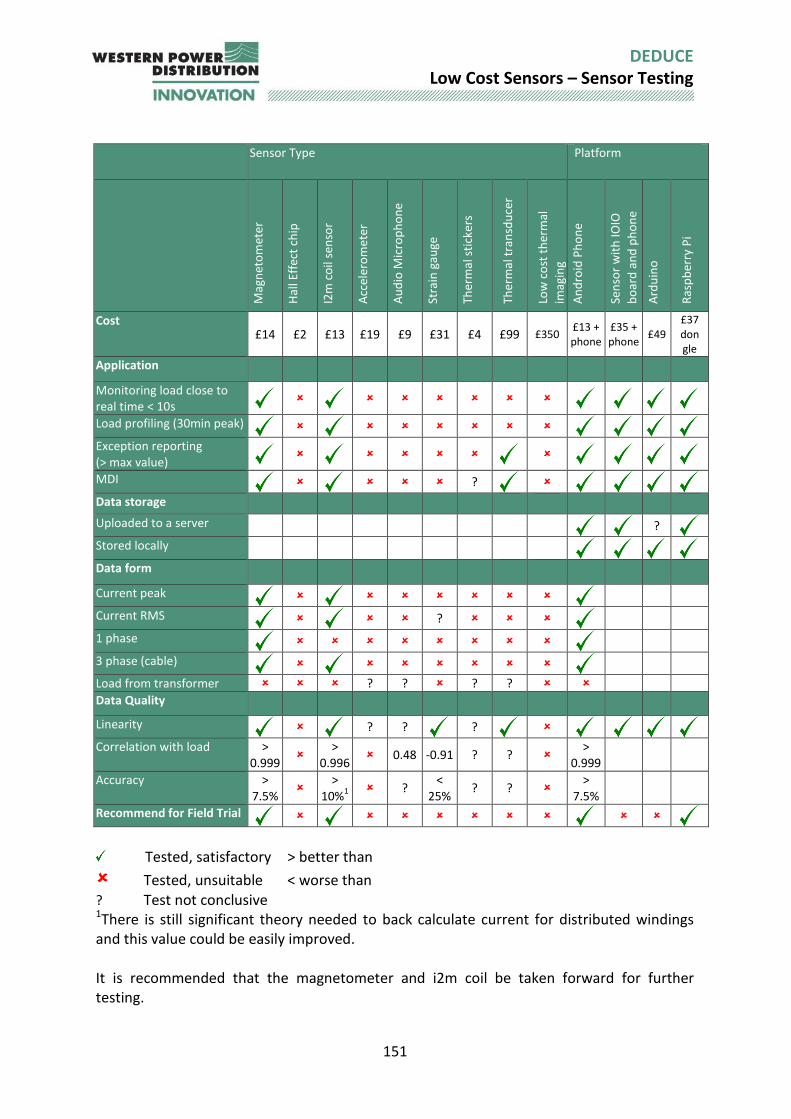
151
DEDUCE Low Cost Sensors – Sensor Testing
Sensor Type Platform
Mag
net
om
eter
Hal
l Eff
ect
chip
I2m
co
il se
nso
r
Acc
eler
om
eter
Au
dio
Mic
rop
ho
ne
Stra
in g
auge
Ther
mal
sti
cker
s
Ther
mal
tra
nsd
uce
r
Low
co
st t
her
mal
imag
ing
An
dro
id P
ho
ne
Sen
sor
wit
h IO
IO
bo
ard
an
d p
ho
ne
Ard
uin
o
Ras
pb
erry
Pi
Cost £14 £2 £13 £19 £9 £31 £4 £99 £350
£13 + phone
£35 + phone
£49 £37 dongle
Application
Monitoring load close to real time < 10s
Load profiling (30min peak)
Exception reporting (> max value)
MDI ?
Data storage
Uploaded to a server ?
Stored locally
Data form
Current peak
Current RMS ?
1 phase
3 phase (cable)
Load from transformer ? ? ? ?
Data Quality
Linearity ? ? ?
Correlation with load > 0.999
>
0.996 0.48 -0.91 ? ?
> 0.999
Accuracy > 7.5%
>
10%1 ?
< 25%
? ? >
7.5%
Recommend for Field Trial
Tested, satisfactory > better than
Tested, unsuitable < worse than ? Test not conclusive 1There is still significant theory needed to back calculate current for distributed windings and this value could be easily improved. It is recommended that the magnetometer and i2m coil be taken forward for further testing.
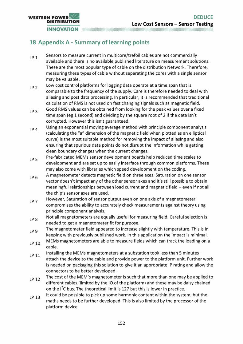
152
DEDUCE Low Cost Sensors – Sensor Testing
18 Appendix A - Summary of learning points
LP 1 Sensors to measure current in multicore/trefoil cables are not commercially available and there is no available published literature on measurement solutions. These are the most popular type of cable on the distribution Network. Therefore, measuring these types of cable without separating the cores with a single sensor may be valuable.
LP 2 Low cost control platforms for logging data operate at a time span that is comparable to the frequency of the supply. Care is therefore needed to deal with aliasing and post data processing. In particular, it is recommended that traditional calculation of RMS is not used on fast changing signals such as magnetic field.
LP 3 Good RMS values can be obtained from looking for the peak values over a fixed time span (eg 1 second) and dividing by the square root of 2 if the data isn’t corrupted. However this isn’t guaranteed.
LP 4 Using an exponential moving average method with principle component analysis (calculating the “a” dimension of the magnetic field when plotted as an elliptical curve) is the most suitable method for removing the impact of aliasing and also ensuring that spurious data points do not disrupt the information while getting clean boundary changes when the current changes.
LP 5 Pre-fabricated MEMs sensor development boards help reduced time scales to development and are set up to easily interface through common platforms. These may also come with libraries which speed development on the coding.
LP 6 A magnetometer detects magnetic field on three axes. Saturation on one sensor vector doesn’t impact any of the other sensor axes and it’s still possible to obtain meaningful relationships between load current and magnetic field – even if not all the chip’s sensor axes are used.
LP 7 However, Saturation of sensor output even on one axis of a magnetometer compromises the ability to accurately check measurements against theory using principle component analysis.
LP 8 Not all magnetometers are equally useful for measuring field. Careful selection is needed to get a magnetometer fit for purpose.
LP 9 The magnetometer field appeared to increase slightly with temperature. This is in keeping with previously published work. In this application the impact is minimal.
LP 10 MEMs magnetometers are able to measure fields which can track the loading on a cable.
LP 11 Installing the MEMs magnetometers at a substation took less than 5 minutes – attach the device to the cable and provide power to the platform unit. Further work is needed on packaging this solution to give it an appropriate IP rating and allow the connectors to be better developed.
LP 12 The cost of the MEM’s magnetometer is such that more than one may be applied to different cables (limited by the IO of the platform) and these may be daisy chained on the I2C bus. The theoretical limit is 127 but this is lower in practice.
LP 13 It could be possible to pick up some harmonic content within the system, but the maths needs to be further developed. This is also limited by the processor of the platform device.
153
DEDUCE Low Cost Sensors – Sensor Testing
LP 14 A hall effect measurement device did not provide a suitable measurement reading to allow output to be correlated to load current.
LP 15 There are many different methods to produce turns or wire onto something suitable to go round a cable. Material with conductive thread could be best for large scale implementation as the coils may be made to tighter specifications in a manufacturing environment (eg straight sides) and these can be easily overlapped for multi-coil designs and stacked to increase the number of turns. In addition waterproofing and adding suitable fastenings eg Velcro could ensure fast installation.
LP 16 The new coil designs were all easily installed either by tape or cable ties. These were then plugged into an amplifier and level shift circuit before connection to a raspberry pi.
LP 17 The new coil designs showed good correlation between measurement and load current in a balanced system.
LP 18 At this stage the maths behind the i2m coil needs further development to take into account factors such as the distributed nature of the windings or the lumping together of the windings and also to look at imbalance.
LP 19 There was no impact on the readings in the presence of a thermal source (heat gun) and only a very small change in value with close by metal work.
LP 20 The coils have to fit 180o around the cable these mean the coils sides have to be a set distance apart. The sewn coil offers the best opportunity for a single design as it can be folded to give the straight edges 180o apart. The PCB and wired coil would need to be made in different sizes for large scale roll out.
LP 21 Although the coil itself can pick up the harmonics. The platform it is connected to may limit the use of this information through the data logging resolution and also timing.
LP 22 The testing undertaken indicated that it was not going to be possible to relate vibration with loading.
LP 23 Even if further testing proved there to be a relationship between loading and vibration under more highly loaded transformers it would require a significant amount of work to develop the maths and calibration process required for large scale roll out. It is unlikely that the calibration procedure could be achieved in a low enough time scale to keep the costs of installation below £50.
LP 24 The testing undertaken indicated that it was not going to be possible to relate noise with loading.
LP 25 Even if further testing proved there to be a relationship between loading and noise under more highly loaded transformers it would require a significant amount of work to develop the maths and calibration process required for large scale roll out. It is unlikely that the calibration procedure could be achieved in a low enough time scale to keep the costs of installation below £50.
LP 26 There would also be challenges involved in capturing the data at a high enough sampling rate to enable a fast Fourier transform to be undertaken to pick up the 100Hz component. None of the low cost platforms had this capability and an FPGA board would probably be required. These are significantly more expensive at the moment but are dropping in price.
LP 27 The long quarter bridge strain gauge was difficult to attach and came loose easily. Therefore, it is not recommended
154
DEDUCE Low Cost Sensors – Sensor Testing
LP 28 The strain gauge did show some correlation between strain gauge measurement and load current. However, this was not very accurate.
LP 29 The quarter bridge strain gauge measurements were less accurate and there was at least one ambiguous data point. This type of strain gauge is not recommended.
LP 30 Calibrating a temperature measurement in one location with or without Utility found equipment does not guarantee calibration in other locations or with other pieces of equipment.
LP 31 Temperature calibration may change due to external influences such as temperature or over time.
LP 32 Thermal stickers are low cost devices that show temperature. However, it is not clear if there is a business case for their use as these would need to be manually observed.
LP 33 A temperature alarm works fine from detection through to received text message. It is an expensive option compared to some of the other sensors and platforms which could offer better data at higher fidelity for lower price.
LP 34 A temperature alarm sensor would not to be calibrated on site – as it is not directly looking for a load current – but would look instead at ensuring that the tank temperature (as a proxy for top oil temperature) did not exceed values set by standards (60oC above 20oC ambient BSEN600-76-2_2011).
LP 35 It should be possible to link a temperature measurement device such a thermistor to a transformer to give an indication of loading. However no representative hardware was available to test properly and calibration on site may be needed.
LP 36 Thermal imaging using an android phone is not going to be suitable as measuring through a conventional camera by changing the filtering couldn’t be made to work.
LP 37 Distance is a factor when turning magnetic field back to an estimate of load current. Therefore, the location of the sensor is important to estimate its distance from the centre of the cable.
LP 38 It works well to use an Android phone as a control platform especially if the internal Magnetometer is being used. However bespoke App software is required to ensure methodology and Readings are transparent.
LP 39 Different phones have different sensors, and these may be in different locations within the phone. If a variety of android types are to be used in large scale testing, then any variance needs to be known so it can be accounted for.
LP 40 There is an obvious relationship between phone magnetometer measurement and current.
LP 41 For early testing the quickest way to attach the phone to the cable was by tape. However, it means the phone is not necessarily the same distance from the centre of the cable and is not always at the same angle. This makes it difficult to test for consistency as distance is a factor. A method of fixing distance was developed to compensate for this.
LP 42 At higher currents saturation may be an issue – However this can be mitigated.
LP 43 Careful placement of the phone can be used to offset issues from saturation. As there are different ratings of substations and different cable types – it may be that a space holder is used for a range of types where angle and distance are carefully matched to rating.
155
DEDUCE Low Cost Sensors – Sensor Testing
LP 44 Using “calibrated” Android phone data can result in factors being arbitrary applied to the measurement at random points in the measurement. This is not so much of an issue for the un-calibrated data which is reported as uncalibrated plus a calibration factor.
LP 45 It is possible to remove the impact of calibration, but this requires post processing or adaptive processing as results are being collected. It is much more straightforward to use the uncalibrated data. However, this can also be adjusted by the phone controller.
LP 46 Android datalogger apps tend to measure with a randomised time interval, so the data must be carefully processed so aliasing effects don’t introduce bias into values.
LP 47 The temporal resolution of measurements on a phone varies from any delay set in code dependent on the processor and other core phone specifications. It is also dependent on what other apps are running and their processor usage.
LP 48 Downloading the data to a server from a mobile phone over Wi-Fi increases the measurement time further and sub 50ms measurement may not be possible.
LP 49 Temperature does not seem to impact the magnetometer reading as the phone is designed to internally compensate for this.
LP 50 Using a phone to calculated load current is possible. There is a good degree of linearity and correlation. The accuracy of the direct back calculation of current from the phone is less than would be liked. However, a lower magnetometer reading shows a higher value of current than would be obtained in the field and therefore there is an inherent safety margin. To get more accurate results a “phone factor” is suggested which could be used to multiply to the calculated current.
LP 51 Calculation on three core and single core cables show different levels of accuracy. This means a phone factor would be required which would depend on cable type.
LP 52 There is some inconsistency between phone types depending on cable type. It could mean that certain phones are more suitable for certain types of cable. This could be related to location and direction of sensor.
LP 53 Installing the phone was the easiest of the sensor installation options. The phone was cable tied to the cable and the phone clipped into place and then App started. A USB power supply was connected to the phone to ensure it didn’t run out of charge.
LP 54 A mobile phone magnetometer was successfully used to log data at a substation on both the LV and HV cable and the data was sent via WI-Fi to a server.
LP 55 An IOIO board offers a neat solution to turn a mobile phone into a controller with up to 60 I/O. It would allow the phone to be connected to any of the sensors under investigation.
LP 56 An Arduino offers an option as a control platform. Shields can be used to provide GPRS interfacing and local data storage. However, the processor size may be a limiting factor.
LP 57 A Raspberry pi is a useful platform for gathering, processing and sending on data. There is sufficient memory to enable an on board database to be set up and the processing of the signals is not as limited by other applications as the mobile phone. The interface to analogue inputs is provided by a low cost chip for which library functions are available.
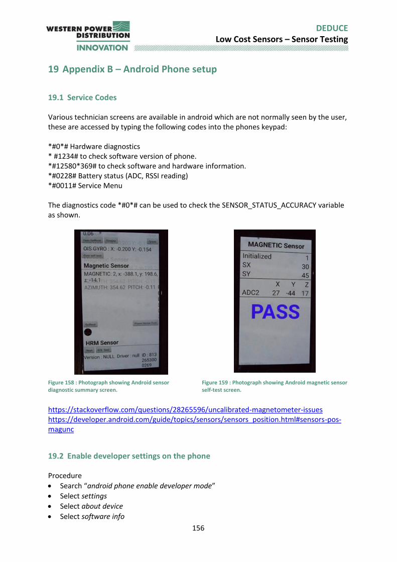
156
DEDUCE Low Cost Sensors – Sensor Testing
19 Appendix B – Android Phone setup
19.1 Service Codes Various technician screens are available in android which are not normally seen by the user, these are accessed by typing the following codes into the phones keypad: *#0*# Hardware diagnostics * #1234# to check software version of phone. *#12580*369# to check software and hardware information. *#0228# Battery status (ADC, RSSI reading) *#0011# Service Menu The diagnostics code *#0*# can be used to check the SENSOR_STATUS_ACCURACY variable as shown.
Figure 158 : Photograph showing Android sensor diagnostic summary screen.
Figure 159 : Photograph showing Android magnetic sensor self-test screen.
https://stackoverflow.com/questions/28265596/uncalibrated-magnetometer-issues https://developer.android.com/guide/topics/sensors/sensors_position.html#sensors-pos-magunc
19.2 Enable developer settings on the phone Procedure
Search “android phone enable developer mode”
Select settings
Select about device
Select software info

157
DEDUCE Low Cost Sensors – Sensor Testing
Select build no and tap this 7 times
This gives developer options at the bottom of the settings menu
Go back to settings
Select developer options
Select USB debugging
Turn this on
19.3 Upload the App to the Phone The software is written in a package called Android Studio To load the software from Android studio to the phone
Plug the USB cable from the computer into the phone
On the menu bar of Android studio there is a picture of a green triangle and a green triangle next to traffic lights. Either will do but the traffic light option allows extra debugging. Click on this
Select deployment target
Select real devices (as opposed to a simulated or emulated device)
Choose the phone from the list and click ok At this point it is probable that extra libraries will be needed (either to deal with the device or Android version or randomly!). The software will tell you it needs to install these. Click ok and the software will download libraries and download software to phone. The phone will launch automatically.
19.4 Using the Deduce App on the phone
Go to settings
Select the site (e.g. Castle Black) ultimately this will be a list of substations
Choose the server – for this report that is bim
Use the slider to move between pause and data capture. A counter increments when data is captured but is difficult to see if this is at too high a rate.
There is a button to delete the readings off the phone (but not the server)
19.5 Viewing the data The server is located at Bim.shef.ac.uk/sensormonitor/view_data.php Select the site and the click refresh Data can be copied and pasted in html or as csv.
158
DEDUCE Low Cost Sensors – Sensor Testing
Information on the sensors can be found at Developer.android.com/reference/android/hardware/sensorevent.html
19.6 Checking the server To ensure the server is ok Go to bim/shef.ac.uk/sensormonitor/sync_test.php Send false readings to the data base to test
Randomise to set a random field
Record to pretend to record this
Upload to upload to the server
Select nothing under server id and when upload is clicked the server selects an ID number and sends it back to appear on the screen.
19.7 Changing the smartphone app Java code The software is version controlled through Github.com There are two versions of code – 1 to set up the server and the other to deal with the phone App. To access the code a login is needed with Github. The login ID needs to be emailed to the software owner so that access to edit may be granted. In Android studio’s
In the menu bar select VCS (version control software)
Select check out from version control under Github
Link to https://github.com/NeilStrickland/sensormonitor_client.git
Select either the sensor monitor server or sensor monitor client and select clone
This downloads into the Android studios and should launch automatically
After changes have been made these can be committed back to Github (little up arrow and in the menu bar)
This is currently under a public repository. A private repository costs $84 pa.
Note: when this is being setup for the first time it will take a while with lots of additional file downloads.
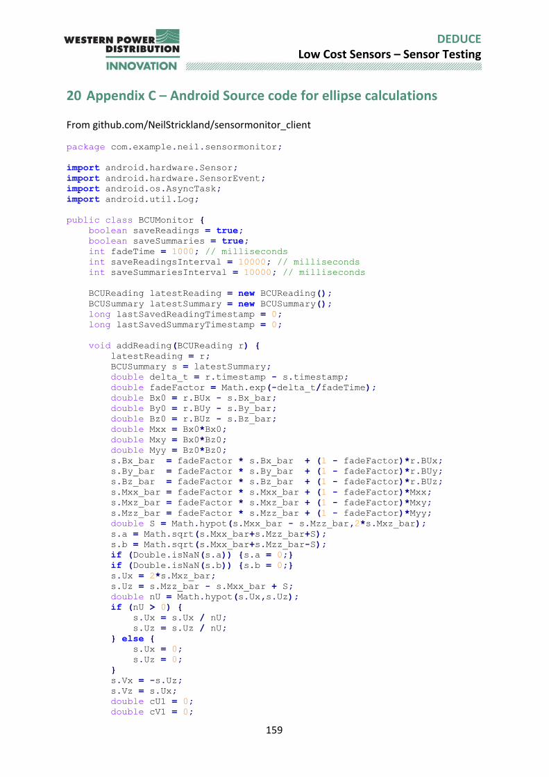
159
DEDUCE Low Cost Sensors – Sensor Testing
20 Appendix C – Android Source code for ellipse calculations From github.com/NeilStrickland/sensormonitor_client
package com.example.neil.sensormonitor;
import android.hardware.Sensor;
import android.hardware.SensorEvent;
import android.os.AsyncTask;
import android.util.Log;
public class BCUMonitor {
boolean saveReadings = true;
boolean saveSummaries = true;
int fadeTime = 1000; // milliseconds
int saveReadingsInterval = 10000; // milliseconds
int saveSummariesInterval = 10000; // milliseconds
BCUReading latestReading = new BCUReading();
BCUSummary latestSummary = new BCUSummary();
long lastSavedReadingTimestamp = 0;
long lastSavedSummaryTimestamp = 0;
void addReading(BCUReading r) {
latestReading = r;
BCUSummary s = latestSummary;
double delta_t = r.timestamp - s.timestamp;
double fadeFactor = Math.exp(-delta_t/fadeTime);
double Bx0 = r.BUx - s.Bx_bar;
double By0 = r.BUy - s.By_bar;
double Bz0 = r.BUz - s.Bz_bar;
double Mxx = Bx0*Bx0;
double Mxy = Bx0*Bz0;
double Myy = Bz0*Bz0;
s.Bx_bar = fadeFactor * s.Bx_bar + (1 - fadeFactor)*r.BUx;
s.By_bar = fadeFactor * s.By_bar + (1 - fadeFactor)*r.BUy;
s.Bz_bar = fadeFactor * s.Bz_bar + (1 - fadeFactor)*r.BUz;
s.Mxx_bar = fadeFactor * s.Mxx_bar + (1 - fadeFactor)*Mxx;
s.Mxz_bar = fadeFactor * s.Mxz_bar + (1 - fadeFactor)*Mxy;
s.Mzz_bar = fadeFactor * s.Mzz_bar + (1 - fadeFactor)*Myy;
double S = Math.hypot(s.Mxx_bar - s.Mzz_bar,2*s.Mxz_bar);
s.a = Math.sqrt(s.Mxx_bar+s.Mzz_bar+S);
s.b = Math.sqrt(s.Mxx_bar+s.Mzz_bar-S);
if (Double.isNaN(s.a)) {s.a = 0;}
if (Double.isNaN(s.b)) {s.b = 0;}
s.Ux = 2*s.Mxz_bar;
s.Uz = s.Mzz_bar - s.Mxx_bar + S;
double nU = Math.hypot(s.Ux,s.Uz);
if (nU > 0) {
s.Ux = s.Ux / nU;
s.Uz = s.Uz / nU;
} else {
s.Ux = 0;
s.Uz = 0;
}
s.Vx = -s.Uz;
s.Vz = s.Ux;
double cU1 = 0;
double cV1 = 0;
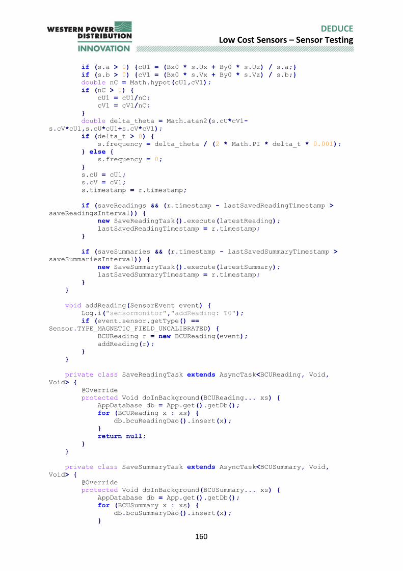
160
DEDUCE Low Cost Sensors – Sensor Testing
if (s.a > 0) {cU1 = (Bx0 * s.Ux + By0 * s.Uz) / s.a;}
if (s.b > 0) {cV1 = (Bx0 * s.Vx + By0 * s.Vz) / s.b;}
double nC = Math.hypot(cU1,cV1);
if (nC > 0) {
cU1 = cU1/nC;
cV1 = cV1/nC;
}
double delta_theta = Math.atan2(s.cU*cV1-
s.cV*cU1,s.cU*cU1+s.cV*cV1);
if (delta_t > 0) {
s.frequency = delta_theta / (2 * Math.PI * delta_t * 0.001);
} else {
s.frequency = 0;
}
s.cU = cU1;
s.cV = cV1;
s.timestamp = r.timestamp;
if (saveReadings && (r.timestamp - lastSavedReadingTimestamp >
saveReadingsInterval)) {
new SaveReadingTask().execute(latestReading);
lastSavedReadingTimestamp = r.timestamp;
}
if (saveSummaries && (r.timestamp - lastSavedSummaryTimestamp >
saveSummariesInterval)) {
new SaveSummaryTask().execute(latestSummary);
lastSavedSummaryTimestamp = r.timestamp;
}
}
void addReading(SensorEvent event) {
Log.i("sensormonitor","addReading: T0");
if (event.sensor.getType() ==
Sensor.TYPE_MAGNETIC_FIELD_UNCALIBRATED) {
BCUReading r = new BCUReading(event);
addReading(r);
}
}
private class SaveReadingTask extends AsyncTask<BCUReading, Void,
Void> {
@Override
protected Void doInBackground(BCUReading... xs) {
AppDatabase db = App.get().getDb();
for (BCUReading x : xs) {
db.bcuReadingDao().insert(x);
}
return null;
}
}
private class SaveSummaryTask extends AsyncTask<BCUSummary, Void,
Void> {
@Override
protected Void doInBackground(BCUSummary... xs) {
AppDatabase db = App.get().getDb();
for (BCUSummary x : xs) {
db.bcuSummaryDao().insert(x);
}
161
DEDUCE Low Cost Sensors – Sensor Testing
return null;
}
}
}
162
DEDUCE Low Cost Sensors – Sensor Testing
21 Appendix D – Arduino Source code used for testing Code for the Arduino Uno and LinkitOne boards was written in a form of C++ using the Arduino IDE on a PC and uploaded to the boards via USB cable. The various digital sensors and other add-on boards (Wi-Fi, LCD display) were selected because open source Arduino libraries are available for them. This meant that they can be setup and controlled with a few lines of code, avoiding the need to send and receive numerous serial data commands. The following libraries were added in the Arduino IDE.
Adafruit_LSM9DS0
Adafruit_Sensor
SparkFunMPU9250-DMP
#include <Wire.h>
#include <SPI.h>
#include <Adafruit_LSM9DS0.h>
#include <Adafruit_Sensor.h>
#include <SparkFunMPU9250-DMP.h>
boolean LSM9DSO_found = false;
boolean MPU9250_found = false;
unsigned long timeNow = 0;
unsigned long mSecInHour = 3600000;
unsigned long TimeNow =0;
int millisecs =0;
int seconds = 0;
byte minutes = 0;
byte hours = 0;
int raw_x;
int raw_y;
int raw_z;
int accel_raw_x;
int accel_raw_y;
int accel_raw_z;
int raw_x_9250;
int raw_y_9250;
int raw_z_9250;
int raw_accel_x_9250;
int raw_accel_y_9250;
int raw_accel_z_9250;
int raw_a0;
int raw_a1;
int raw_a2;
// i2c
Adafruit_LSM9DS0 lsm = Adafruit_LSM9DS0();
// You can also use software SPI
//Adafruit_LSM9DS0 lsm = Adafruit_LSM9DS0(13, 12, 11, 10, 9);
// Or hardware SPI! In this case, only CS pins are passed in
//Adafruit_LSM9DS0 lsm = Adafruit_LSM9DS0(10, 9);
163
DEDUCE Low Cost Sensors – Sensor Testing
MPU9250_DMP imu;
void setupSensor()
{
// 1.) Set the accelerometer range (2G,4G,6G,8G,16G )
lsm.setupAccel(lsm.LSM9DS0_ACCELRANGE_2G);
// 2.) Set the magnetometer sensitivity (2GAUSS,4GAUSS,8GAUSS,12GAUSS)
lsm.setupMag(lsm.LSM9DS0_MAGGAIN_12GAUSS);
// 3.) Setup the gyroscope (245DPS,500DPS,2000DPS)
// lsm.setupGyro(lsm.LSM9DS0_GYROSCALE_245DPS);
}
void setup()
{
pinMode(A0, INPUT);
pinMode(A1, INPUT);
pinMode(A2, INPUT);
#ifndef ESP8266
while (!Serial); // will pause Zero, Leonardo, etc until serial
console opens
#endif
Serial.begin(9600);
// Try to initialise and warn if we couldn't detect the chip
if (!lsm.begin())
{
Serial.println(F("Oops ... unable to initialize the LSM9DS0. Check
your wiring!"));
while (1); { Serial.println(F("Found LSM9DS0 9DOF, measurements in
Gauss"));}
}
else
{
LSM9DSO_found = true;
}
// if (imu.begin() != INV_SUCCESS)
// { while (1) { Serial.println("No MPU-9250 found, Check
connections"); }
// imu.setSensors(INV_XYZ_ACCEL | INV_XYZ_COMPASS); // Enable chosen
sensors:
// imu.setAccelFSR(2); // Set accel = +/-2g (2, 4, 8, 16g allowed) FSR is
+/- 4912 uT
// imu.setLPF(188); // Set accel & gyro LPF corner freq 188, 98, 42, 20,
10, 5 Hz allowed
// imu.setSampleRate(4); // Set accel/gyro sample rate 4Hz to 1kHz
allowed
// imu.setCompassSampleRate(1); // Set mag sample rate (1-100Hz allowed)
// MPU9250_found = true;
// }
Serial.println(F("MilliSecsApprox,TimeElapsed, mag_x, mag_y, mag_z, "));
Serial.println(F("accel_x, accel_y, accel_z, a0, a1, a2 "));
Serial.println(F(""));
}
void loop()
{
164
DEDUCE Low Cost Sensors – Sensor Testing
TimeNow = millis();
hours = TimeNow/mSecInHour;
minutes = (TimeNow-(hours*mSecInHour))/(mSecInHour/60);
seconds = (TimeNow-(hours*mSecInHour)-(minutes*(mSecInHour/60)))/1000;
millisecs = TimeNow-(hours*mSecInHour)-(minutes*(mSecInHour/60))-
(seconds*1000);
// lsm.read();
// if ( imu.dataReady() )
// { imu.update(UPDATE_ACCEL | UPDATE_COMPASS);}
// raw_x = lsm.magData.x;
// raw_y = lsm.magData.y;
// raw_z = lsm.magData.z;
// accel_raw_x = lsm.accelData.x;
// accel_raw_y = lsm.accelData.y;
// accel_raw_z = lsm.accelData.z;
if (MPU9250_found)
{
raw_x_9250 = 1000 * imu.calcMag(imu.mx);
raw_y_9250 = 1000 * imu.calcMag(imu.my);
raw_z_9250 = 1000 * imu.calcMag(imu.mz);
raw_accel_x_9250 = 1000 * imu.calcAccel(imu.ax);
raw_accel_y_9250 = 1000 * imu.calcAccel(imu.ay);
raw_accel_z_9250 = 1000 * imu.calcAccel(imu.az);
}
raw_a0 = analogRead(A0);
raw_a1 = analogRead(A1);
raw_a2 = analogRead(A2);
Serial.print(TimeNow);
Serial.print(", ");
Serial.print(hours);
Serial.print(":");
Serial.print(minutes);
Serial.print(":");
Serial.print(seconds);
Serial.print(".");
if (millisecs<100) // need to add leading zeros for fractional
millisecs
{ Serial.print("0"); }
if (millisecs<10)
{ Serial.print("0"); }
Serial.print(millisecs);
Serial.print(", ");
if (LSM9DSO_found)
{
Serial.print((int) (raw_x) ); Serial.print(F(", "));
Serial.print((int) (raw_y) ); Serial.print(F(", "));
Serial.print((int) (raw_z) ); Serial.print(F(", "));
Serial.print((int) (accel_raw_x) ); Serial.print(F(", "));
Serial.print((int) (accel_raw_y) ); Serial.print(F(", "));
Serial.print((int) (accel_raw_z) ); Serial.print(F(", "));
}
else { Serial.print("-9999,-9999,-9999,-9999,-9999,-9999,");}
165
DEDUCE Low Cost Sensors – Sensor Testing
if (MPU9250_found)
{
Serial.print((int) (raw_x_9250) ); Serial.print(F(", "));
Serial.print((int) (raw_y_9250) ); Serial.print(F(", "));
Serial.print((int) (raw_z_9250) ); Serial.print(F(", "));
Serial.print((int) (raw_accel_x_9250) ); Serial.print(F(", "));
Serial.print((int) (raw_accel_y_9250) ); Serial.print(F(", "));
Serial.print((int) (raw_accel_z_9250) ); Serial.print(F(", "));
}
else { Serial.print("-9999,-9999,-9999,-9999,-9999,-9999,");}
Serial.print((int) (raw_a0) ); Serial.print(F(", "));
Serial.print((int) (raw_a1) ); Serial.print(F(", "));
Serial.print((int) (raw_a2) ); Serial.print(F(" "));
Serial.println(F(""));
}
166
DEDUCE Low Cost Sensors – Sensor Testing
22 Appendix E – Raspberry Pi code import math
import time
import datetime
import threading
import mysql.connector
import RPi.GPIO as GPIO
import Adafruit_GPIO.SPI as SPI
import Adafruit_MCP3008
def current_timestamp():
epoch = datetime.datetime.utcfromtimestamp(0)
current_datetime = datetime.datetime.now()
return round((current_datetime - epoch).total_seconds() *
1000.0)
class SensorMonitor:
def __init__(self):
self.site_id = 1
self.BCU_reading_site_id = 0
self.watcher = None
self.connection = None
self.cursor = None
self.mcp = None
self.current_BCU_summary = BCU_summary()
self.current_BCU_summary.site_id = self.site_id
def GPIO_setup(self):
# Software SPI configuration:
# note this software sets the GPIO mode to be GPIO pin
related
CLK = 18
MISO = 23
MOSI = 24
CS = 25
self.mcp = Adafruit_MCP3008.MCP3008(clk=CLK, cs=CS,
miso=MISO, mosi=MOSI)
#set GPIO pin 4 - physical pin 7 to be a push button input
GPIO.setup(4, GPIO.IN, pull_up_down=GPIO.PUD_DOWN)
#set GPIO 21- physical pin 40 as an LED output - to go high
when recording
GPIO.setup(21,GPIO.OUT)
def GPIO_start(self):
#detect when this has been pushed and if so call logging
routine
GPIO.add_event_detect(4,GPIO.RISING,callback=self.handle_button)
def database_setup(self):
167
DEDUCE Low Cost Sensors – Sensor Testing
self.connection =
mysql.connector.connect(user='sensormonitor',
password='qvZ5nINAfHJvYlaq',
host='localhost',
database='sensormonitor')
self.cursor = self.connection.cursor()
def next_BCU_reading_site_id(self):
i = self.BCU_reading_site_id
self.BCU_reading_site_id = i+1
return i+1
def take_BCU_reading(self):
r = BCU_reading()
r.read(self.mcp)
r.site_id = self.site_id
r.site_record_id = self.next_BCU_reading_site_id()
return r
def handle_button(self,channel):
print("Button was pushed!")
if self.watcher is None:
print("Starting")
self.watcher = Watcher(self)
self.watcher.start()
else:
print("Stopping")
self.watcher.stop()
self.watcher.join()
self.watcher = None
class BCU_reading:
add_query = ("INSERT INTO tbl_BCU_readings"
"(site_id,site_record_id,timestamp,BUx,BUy,BUz)"
"VALUES (%s, %s, %s, %s, %s,%s)")
fmt = '| {0:>6} | {1:>6} | {2:>6} | {3:>9} | {4:>4} | {5:>4} |
{6:>4} |'
def __init__(self):
self.id = 0
self.site_id = 0
self.site_record_id = 0
self.timestamp = 0
self.BUx = 0
self.BUy = 0
self.BUz = 0
def read(self,mcp):
self.timestamp = current_timestamp()
self.BUx = mcp.read_adc(0)
self.BUy = mcp.read_adc(1)
self.BUz = mcp.read_adc(2)
def save(self,cursor):
168
DEDUCE Low Cost Sensors – Sensor Testing
values=(self.site_id,self.site_record_id,self.timestamp,
self.BUx,self.BUy,self.BUz)
cursor.execute(self.add_query,values)
self.id = cursor.lastrowid
def show(self):
print(self.fmt.format(self.id,self.site_id,self.site_record_id,self.
timestamp,
self.BUx,self.BUy,self.BUz))
class BCU_summary:
add_query = ("INSERT INTO tbl_BCU_summaries"
"(site_id,site_record_id,timestamp,Bx_bar,By_bar,Bz_bar,Mxx_bar,Mxz_
bar,Mzz_bar,a,b,Ux,Uz,Vx,Vz,cU,cV,frequency)"
"VALUES (%s, %s, %s, %s, %s, %s, %s, %s, %s, %s, %s, %s,
%s, %s, %s, %s, %s, %s)")
fmt = '| {0:>6} | {1:>6} | {2:>6} | {3:>9} | {4:>4} | {5:>4} |
{6:>4} |{7:>4} |{8:>4} | {9:>4} |{10:>4} |{11:>4} |{12:>4} |{13:>4}
|{14:>4} |{15:>4} |{16:>4} |{17:>4} |{18:>4} |'
def __init__(self):
self.fadeTime = 1000.0 # milliseconds
self.id = 0
self.site_id = 0
self.site_record_id = 0
self.timestamp = 0
self.Bx_bar = 0
self.By_bar = 0
self.Bz_bar = 0
self.Mxx_bar = 0
self.Mxz_bar = 0
self.Mzz_bar = 0
self.a = 0
self.b = 0
self.Ux = 0
self.Uz = 0
self.Vx = 0
self.Vz = 0
self.cU = 0
self.cV = 0
self.frequency = 0
self.BUx=0
self.BUy=0
self.BUz=0
self.last_save_time = current_timestamp()
self.save_interval = 10000 # milliseconds
self.latest_reading = None
def add_reading(self,r):
self.latest_reading = r
delta_t = r.timestamp - self.timestamp
fadeFactor = math.exp(-delta_t/self.fadeTime)
169
DEDUCE Low Cost Sensors – Sensor Testing
Bx0 = r.BUx - self.Bx_bar
By0 = r.BUy - self.By_bar
Bz0 = r.BUz - self.Bz_bar
Mxx = Bx0*Bx0
Mxy = Bx0*Bz0
Myy = Bz0*Bz0
self.Bx_bar = fadeFactor * self.Bx_bar + (1 -
fadeFactor)*r.BUx
self.By_bar = fadeFactor * self.By_bar + (1 -
fadeFactor)*r.BUy
self.Bz_bar = fadeFactor * self.Bz_bar + (1 -
fadeFactor)*r.BUz
self.Mxx_bar = fadeFactor * self.Mxx_bar + (1 -
fadeFactor)*Mxx
self.Mxz_bar = fadeFactor * self.Mxz_bar + (1 -
fadeFactor)*Mxy
self.Mzz_bar = fadeFactor * self.Mzz_bar + (1 -
fadeFactor)*Myy
S = math.hypot(self.Mxx_bar - self.Mzz_bar,2*self.Mxz_bar)
self.a = math.sqrt(self.Mxx_bar+self.Mzz_bar+S)
self.b = math.sqrt(self.Mxx_bar+self.Mzz_bar-S)
if (math.isnan(self.a)):
self.a = 0
if (math.isnan(self.b)):
self.b = 0
self.Ux = 2*self.Mxz_bar
self.Uz = self.Mzz_bar - self.Mxx_bar + S
nU = math.hypot(self.Ux,self.Uz)
if (nU > 0):
self.Ux = self.Ux / nU
self.Uz = self.Uz / nU
else:
self.Ux = 0
self.Uz = 0
self.Vx = -self.Uz
self.Vz = self.Ux
cU1 = 0
cV1 = 0
if (self.a > 0):
U1 = (Bx0 * self.Ux + By0 * self.Uz) / self.a
if (self.b > 0):
cV1 = (Bx0 * self.Vx + By0 * self.Vz) / self.b
nC = math.hypot(cU1,cV1)
if (nC > 0):
cU1 = cU1/nC
cV1 = cV1/nC
delta_theta = math.atan2(self.cU*cV1-
self.cV*cU1,self.cU*cU1+self.cV*cV1)
if (delta_t > 0):
self.frequency = delta_theta / (2 * math.pi * delta_t *
0.001)
else:
self.frequency = 0
self.cU = cU1
self.cV = cV1
170
DEDUCE Low Cost Sensors – Sensor Testing
self.timestamp = r.timestamp
def should_save(self):
return ((self.timestamp - self.last_save_time) >
self.save_interval)
def save(self,cursor):
self.site_record_id = self.site_record_id + 1
values=(self.site_id,self.site_record_id,self.timestamp,
self.Bx_bar,self.By_bar,self.Bz_bar,self.Mxx_bar,
self.Mxz_bar,self.Mzz_bar,self.a,self.b,self.Ux,
self.Uz,self.Vx,self.Vz,self.cU,self.cV,self.frequency)
cursor.execute(self.add_query,values)
self.id = cursor.lastrowid
self.last_save_time = current_timestamp()
def show(self):
print(self.fmt.format(self.id,self.site_id,self.site_record_id,self.
timestamp,
self.Bx_bar,self.By_bar,self.Bz_bar,self.Mxx_bar,
self.Mxz_bar,self.Mzz_bar,self.a,self.b,self.Ux,
self.Uz,self.Vx,self.Vz,self.cU,self.cV,self.frequency))
class Watcher(threading.Thread):
def __init__(self,monitor):
super(Watcher, self).__init__()
self.monitor = monitor
self._stop_event = threading.Event()
def stop(self):
self._stop_event.set()
def stopped(self):
return self._stop_event.is_set()
def run(self):
while (not self._stop_event.is_set()):
GPIO.output(21,1)
m = self.monitor
r = m.take_BCU_reading()
r.save(m.cursor)
r.show()
s = m.current_BCU_summary
s.add_reading(r)
if s.should_save():
s.save(m.cursor)
s.show()
GPIO.output(21,0)
def handle_button(channel):
171
DEDUCE Low Cost Sensors – Sensor Testing
global watcher
print("Button was pushed!")
if watcher is None:
print("Starting")
watcher = Watcher()
watcher.start()
else:
print("Stopping")
watcher.stop()
watcher.join()
watcher = None
sm = SensorMonitor()
sm.database_setup()
sm.GPIO_setup()
print('Reading MCP3008 values, press Ctrl-C to quit...')
print('-' * 57)
current_datetime = datetime.datetime.now()
print ("Current time %s" % current_datetime)
sm.GPIO_start()
while True:
time.sleep(10)
172
DEDUCE Low Cost Sensors – Sensor Testing
23 Appendix F – IOIO board code package ioio.examples.simple; import ioio.lib.api.AnalogInput; import ioio.lib.api.DigitalOutput; import ioio.lib.api.IOIO; import ioio.lib.api.PwmOutput; import ioio.lib.api.exception.ConnectionLostException; import ioio.lib.util.BaseIOIOLooper; import ioio.lib.util.IOIOLooper; import ioio.lib.util.android.IOIOActivity; import android.os.Bundle; import android.widget.SeekBar; import android.widget.TextView; import android.widget.ToggleButton; public class IOIOSimpleApp extends IOIOActivity { private TextView textView_; private SeekBar seekBar_; private ToggleButton toggleButton_; @Override public void onCreate(Bundle savedInstanceState) { super.onCreate(savedInstanceState); setContentView(R.layout.main); textView_ = (TextView) findViewById(R.id.TextView); seekBar_ = (SeekBar) findViewById(R.id.SeekBar); toggleButton_ = (ToggleButton) findViewById(R.id.ToggleButton); enableUi(false); } class Looper extends BaseIOIOLooper { private AnalogInput input_; private PwmOutput pwmOutput_; private DigitalOutput led_; @Override public void setup() throws ConnectionLostException { led_ = ioio_.openDigitalOutput(IOIO.LED_PIN, true); input_ = ioio_.openAnalogInput(40); pwmOutput_ = ioio_.openPwmOutput(12, 100); enableUi(true);
173
DEDUCE Low Cost Sensors – Sensor Testing
} @Override public void loop() throws ConnectionLostException, InterruptedException { setNumber(input_.getVoltage()); pwmOutput_.setPulseWidth(500 + seekBar_.getProgress() * 2); led_.write(!toggleButton_.isChecked()); Thread.sleep(10); } @Override public void disconnected() { enableUi(false); } } @Override protected IOIOLooper createIOIOLooper() { return new Looper(); } private void enableUi(final boolean enable) { runOnUiThread(new Runnable() { @Override public void run() { seekBar_.setEnabled(enable); toggleButton_.setEnabled(enable); } }); } private void setNumber(float f) { final String str = String.format("%.4f", f); runOnUiThread(new Runnable() { @Override public void run() { textView_.setText(str); } }); } }