Embed Size (px)
Citation preview
Decomposition of the mean difference
of a linear combination of variates∗
Paolo Radaelli - Michele Zenga†
Dipartimento di Metodi Quantitativi
per le Scienze Economiche ed Aziendali
Universita degli Studi di Milano-Bicocca
1 Introduction
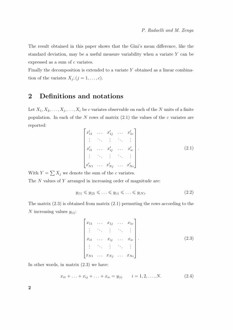
In this paper we show, in an elementary way, that the mean difference of the sum
Y of the variates X1, X2, . . . , Xj, . . . , Xc, can be obtained as the difference of the
sum of the mean differences of each variate Xj with a non-negative quantity that
measures the departure of the data matrix from the uniform ranking (cograduation)
matrix. The mean difference ∆(Y ) of Y is equal to the sum∑
∆ (Xj) of the mean
differences of each variate Xj only if there is a “uniform ranking” among the varia-
tes.
By utilizing the decomposition of ∆ (Y ) we have decomposed, in an analogous way,
the Gini’s concentration ratio of a sum of non-negative variates.
∗A previous version of this work can be found in Zenga and Radaelli [2002] and has been
presented at the Fourth International Conference on Statistical Data Analysis based on the L1-
Norm and Related Methods - University of Neuchatel, Switzerland, see Radaelli and Zenga [2002].†The present work reflects the common thinking of the two authors, even if, more specifically,
M. Zenga wrote sections 1, 2 and 3, while P. Radaelli wrote the remaining sections.
1
P. Radaelli and M. Zenga
The result obtained in this paper shows that the Gini’s mean difference, like the
standard deviation, may be a useful measure variability when a variate Y can be
expressed as a sum of c variates.
Finally the decomposition is extended to a variate Y obtained as a linear combina-
tion of the variates Xj; (j = 1, . . . , c).
2 Definitions and notations
Let X1, X2, . . . , Xj, . . . , Xc be c variates observable on each of the N units of a finite
population. In each of the N rows of matrix (2.1) the values of the c variates are
reported:
x′11 . . . x′
1j . . . x′1c
.... . .
.... . .
...
x′i1 . . . x′
ij . . . x′ic
.... . .
.... . .
...
x′N1 . . . x′
Nj . . . x′Nc
. (2.1)
With Y =∑
Xj we denote the sum of the c variates.
The N values of Y arranged in increasing order of magnitude are:
y(1) 6 y(2) 6 . . . 6 y(i) 6 . . . 6 y(N). (2.2)
The matrix (2.3) is obtained from matrix (2.1) permuting the rows according to the
N increasing values y(i):
x11 . . . x1j . . . x1c
.... . .
.... . .
...
xi1 . . . xij . . . xic
.... . .
.... . .
...
xN1 . . . xNj . . . xNc
. (2.3)
In other words, in matrix (2.3) we have:
xi1 + . . . + xij + . . . + xic = y(i) i = 1, 2, . . . , N. (2.4)
2
Decomposition of the mean difference of a linear combination of variates
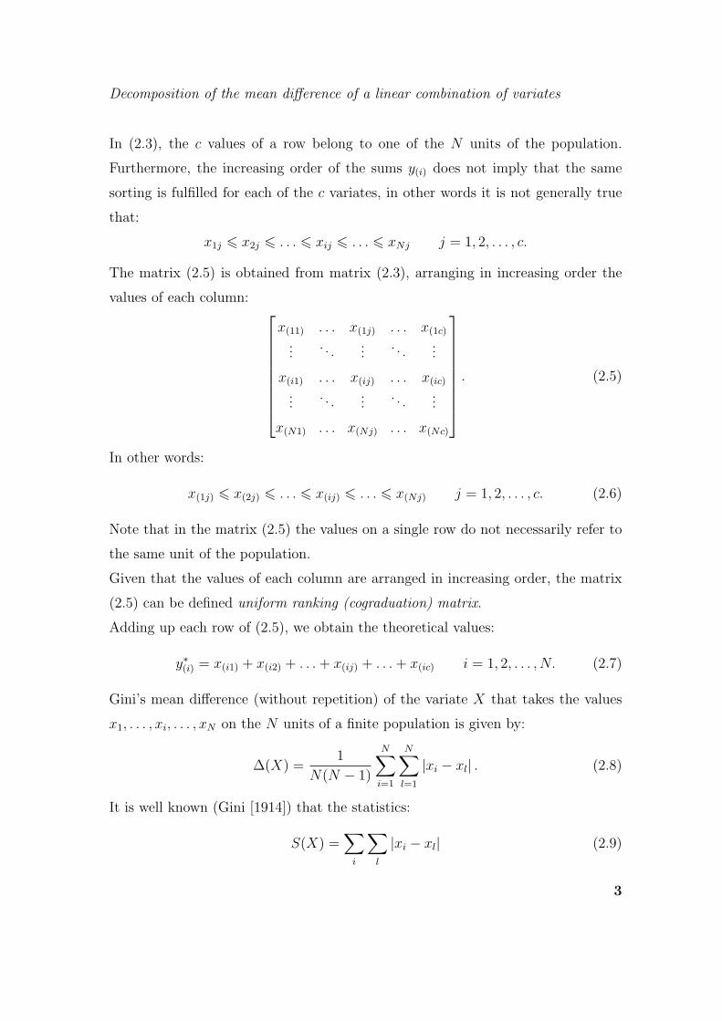
In (2.3), the c values of a row belong to one of the N units of the population.
Furthermore, the increasing order of the sums y(i) does not imply that the same
sorting is fulfilled for each of the c variates, in other words it is not generally true
that:
x1j 6 x2j 6 . . . 6 xij 6 . . . 6 xNj j = 1, 2, . . . , c.
The matrix (2.5) is obtained from matrix (2.3), arranging in increasing order the
values of each column:
x(11) . . . x(1j) . . . x(1c)
.... . .
.... . .
...
x(i1) . . . x(ij) . . . x(ic)
.... . .
.... . .
...
x(N1) . . . x(Nj) . . . x(Nc)
. (2.5)
In other words:
x(1j) 6 x(2j) 6 . . . 6 x(ij) 6 . . . 6 x(Nj) j = 1, 2, . . . , c. (2.6)
Note that in the matrix (2.5) the values on a single row do not necessarily refer to
the same unit of the population.
Given that the values of each column are arranged in increasing order, the matrix
(2.5) can be defined uniform ranking (cograduation) matrix.
Adding up each row of (2.5), we obtain the theoretical values:
y∗(i) = x(i1) + x(i2) + . . . + x(ij) + . . . + x(ic) i = 1, 2, . . . , N. (2.7)
Gini’s mean difference (without repetition) of the variate X that takes the values
x1, . . . , xi, . . . , xN on the N units of a finite population is given by:
∆(X) =1
N(N − 1)
N∑i=1
N∑l=1
|xi − xl| . (2.8)
It is well known (Gini [1914]) that the statistics:
S(X) =∑
i
∑l
|xi − xl| (2.9)
3

P. Radaelli and M. Zenga
is given by:
S(X) = 2∑
i
x(i)(2i − N − 1). (2.10)
3 Decomposition of the mean difference of a sum
The mean difference of the variate Y =∑
Xj is given by:
∆(Y ) =S(Y )
N(N − 1)(3.1)
where, according to (2.10):
S(Y ) =∑
i
∑l
|yi − yl| = 2∑
i
y(i)(2i − N − 1). (3.2)
Substituting (2.4) in (3.2) we have:
S(Y ) =2N∑
i=1
(c∑
j=1
xij
)(2i − N − 1)
=∑
j
2∑
i
xij(2i − N − 1). (3.3)
We can rewrite (3.3) as follows:
S(Y ) =∑
j
2∑
i
(x(ij) − x(ij) + xij
)(2i − N − 1)
=∑
j
2∑
i
x(ij)(2i − N − 1) − 2∑
j
∑i
(x(ij) − xij
)(2i − N − 1). (3.4)
From (2.10):
S(Xj) = 2N∑
i=1
x(ij)(2i − N − 1),
thus:
S(Y ) =∑
j
S(Xj) − 2∑
j
∑i
(x(ij) − xij
)(2i − N − 1). (3.5)
The sum∑
j
∑i
(x(ij) − xij
)(2i − N − 1) is equal to:
= 2∑
j
∑i
(x(ij) − xij
)i − (N + 1)
∑j
∑i
(x(ij) − xij
).
4

Decomposition of the mean difference of a linear combination of variates
Now, since the sum∑
i
(x(ij) − xij
)= 0, for each j = 1, 2, . . . , c, it derives that:∑
j
∑i
(x(ij) − xij
)(2i − N − 1) = 2
∑j
∑i
(x(ij) − xij
)i
and, substituting in (3.5), we get:
S(Y ) =∑
j
S(Xj) − 4∑
j
∑i
(x(ij) − xij
)i. (3.6)
By theorem 368 of Hardy et al. [1952, p. 261], the sum:
N∑i=1
i xij
is greatest when the values xij, i = 1, . . . , N are arranged in increasing order, that
is:N∑
i=1
i xij 6N∑
i=1
i x(ij).
Therefore, for each j = 1, . . . , c, we have:∑i
(x(ij) − xij
)i > 0 (3.7)
with equality only if xij = x(ij), i = 1, . . . N .
It derives that: ∑j
∑i
(x(ij) − xij
)i > 0 (3.8)
with equality only if xij = x(ij) ∀i, j; that is when the matrix (2.3) is equal to the
uniform ranking matrix (2.5).
From (3.6) and (3.8) we get:
S(Y ) = S(X1 + X2 + . . . + Xc) 6∑
j
S(Xj). (3.9)
The non-negative term 4∑
j
∑i
(x(ij) − xij
)i can be interpreted as a measure of
departure of the data matrix (2.3) from the uniform ranking (cograduation) matrix
(2.5).
5

P. Radaelli and M. Zenga
Dividing (3.6) by N(N − 1) we obtain the subtractive decomposition for the Gini’s
mean difference of Y :
∆(Y ) = ∆(X1 + . . . + Xc) =∑
j
∆(Xj) −4
N(N − 1)
∑j
∑i
(x(ij) − xij
)i. (3.10)
Obviously:
∆(Y ) = ∆(X1 + X2 + . . . + Xc) 6∑
j
∆(Xj) (3.11)
with equality only in the case of uniform ranking of the c variates.
Zenga [2003] derived from decomposition (3.10) the following normalized distribu-
tive compensation index:
C = 1 − ∆(Y )∑cj=1 ∆(Xj)
= 1 − S(Y )∑cj=1 S(Xj)
whose range is [0; 1] in particular:
C = 0 if there is no compensation among the c variates i.e. there is uniform ranking
(co-graduation);
C = 1 if there is maximum compensation among the c variates i.e. Y is constantly
equal to M1(Y ).
The compensation index C was also investigated by Maffenini [2003] who decompo-
ses C in order to evaluate the contribution of each variate to the overall compensa-
tion; furthermore the author studies the index behaviour in the case of independence
among the variates and applies the methodology to italian families incomes.
Moreover Borroni and Zenga [2003] propose a test of concordance based on the di-
stributive compensation ratio C and compare it with other classical rank correlation
methods such as the Spearman’s rho and the Kendall’s tau. Some developments on
the power of this test are the object of the investigation by Borroni and Cazzaro
[2005].
6

Decomposition of the mean difference of a linear combination of variates
4 Decomposition of Gini’s concentration ratio of
a sum
In this section we assume that the c variates Xj are non-negative and that their
mean values are positive:
M1 (Xj) =1
N
∑i
xij > 0 j = 1, 2, . . . , c. (4.1)
Obviously:
M1(Y ) =∑
j
M1(Xj) > 0. (4.2)
Gini’s concentration ratio of a non-negative variate X with M1(X) > 0, is defined
by:
R(X) =∆(X)
2M1(X). (4.3)
Dividing both terms in (3.10) by 2M1(Y ), we obtain:
R(Y ) =∆(Y )
2M1(Y )
=∆(X1) + . . . + ∆(Xc)
2M1(Y )− 4
2M1(Y )N(N − 1)
∑j
∑i
(x(ij) − xij
)i
=
∆(X1)
2M1(X1)2M1(X1) + . . . +
∆(Xc)
2M1(Xc)2M1(Xc)
2M1(Y )−
2∑∑(
x(ij) − xij
)i
M1(Y )N(N − 1)
=R(X1)M1(X1) + . . . + R(Xc)M1(Xc)
M1(X1) + . . . + M1(Xc)−
2∑∑(
x(ij) − xij
)i
M1(Y )N(N − 1).
The share of the variate Xj on the sum Y is given by:
ωj =
∑i xij∑
j
∑i xij
=NM1(Xj)
NM1(Y )=
M1(Xj)
M1(Y ); (4.4)
obviously∑
j ωj = 1.
Thus the decomposition of R(Y ) can be rewritten as:
R(Y ) =∑
j
R (Xj) ωj −2
N(N − 1)M1(Y )
∑j
∑i
(x(ij) − xij
)i. (4.5)
7

P. Radaelli and M. Zenga
Equation (4.5) is an easy decomposition that allows Gini’s concentration ratio of
a sum to be obtained as the difference of the weighted arithmetic mean of concen-
tration ratios of each variate Xj with a non-negative quantity that measures the
departure of the data matrix (2.3) from the uniform ranking (cograduation) matrix
(2.5).
5 Comparison with others Gini’s concentration
ratio decompositions
5.1 The decomposition proposed by Rao
Rao [1969] proposed two decompositions of Gini’s concentration ratio: the first one
is by sub-populations, the second one is by components of income1. In this section
we compare the latter with the decomposition (4.5).
Let xij be the income of the i−th family (i = 1, . . . , N) due to the j−th component
Xj (j = 1, . . . , c). The total income of the i − th family is given by: yi =∑
j xij.
The whole income composition of the N families can be reported in a matrix similar
to (2.1).
Suppose to permute the rows of the matrix (2.1) so that the families are arranged
in increasing order according to their total incomes y(i) (matrix (2.3)).
The objective of this approach is to explain the inequality of total incomes by the
inequalities observable for each of the c income sources. In order to reach this result,
Rao considers, for each income component, two different sortings of the N families:
i) in the first one the values of each income component are sorted in increasing
order of magnitude; in other words for the j − th component we have:
x(1j) 6 . . . 6 x(ij) 6 . . . 6 x(Nj)
1The subject is also discussed in Kakwani [1980].
8

Decomposition of the mean difference of a linear combination of variates
The result is a uniform ranking (cograduation) matrix (2.5);
ii) in the second one the income components are sorted in increasing order ac-
cording to their total incomes (matrix (2.3)).
The families are then partitioned, for both sortings, in k subsets so that each set
includes N/k families.
In order to make the comparison with decomposition (4.5) easier we set k = N so
that each subset includes only one family.
Let
•
q′ij =i∑
t=1
xtj i = 1, . . . , N
indicate the cumulative sums of the j−th component incomes in matrix (2.3);
•
q′ij =i∑
t=1
x(tj) i = 1, . . . , N
be the same cumulative sums in matrix (2.5).
The value of Gini’s concentration ratio for the j − th income component (j − th
column of matrix (2.5)) R(Xj) = ∆(Xj)/2M1(Xj) can be obtained by the following
formula related to the Lorenz curve (Gini [1914]):
R(Xj) =
∑N−1i=1
(i M1(Xj) − q′ij
)∑N−1i=1 i M1(Xj)
=
∑N−1i=1 (pi − qij)∑N−1
i=1 pi
(5.1)
where pi =i
Nand qij =
q′ijN M1(Xj)
.
Rao applies formula (5.1) also on the cumulative sums q′ij obtaining the statistics:
R(Xj) =
∑N−1i=1
(i M1(Xj) − q′ij
)∑N−1i=1 i M1(Xj)
=
∑N−1i=1 (pi − qij)∑N−1
i=1 pi
(5.2)
where qij =q′ij
N M1(Xj).
9

P. Radaelli and M. Zenga
Note that R(Xj) is not Gini’s concentration ratio since the N values xij in a column
of matrix (2.3) are not necessarily in increasing order.2
Furthermore Rao shows that:
−R(Xj) 6 R(Xj) 6 R(Xj) (5.3)
where the lower and the upper bounds are reached respectively if in the j − th
column of matrix (2.3) the N families j− th incomes are in descending or ascending
order.
Rao shows that the concentration ratio R(Y ), computed on the total incomes,
can be obtained as the difference of the weighted arithmetic mean of components
concentration ratios, with weights given by the shares (4.4) of each component on
the total income, with a non-negative quantity that Rao defined “an overall measure
of the extent to which component-inequalities offset each other”. Using the notation
above, Rao’s decomposition is:
R(Y ) =∑
j
R(Xj) ωj −∑
j
R(Xj) ωj
[1 − R(Xj)
R(Xj)
]. (5.4)
Comparing decompositions (4.5) and (5.4) we note that, for both, we have to sub-
tract a non-negative term from the weighted arithmetic mean of concentration ratios
computed on each income component. These terms are respectively:
2
N(N − 1)M1(Y )
∑j
∑i
(x(ij) − xij
)i (5.5)
and: ∑R(Xj) ωj
[1 − R(Xj)
R(Xj)
]. (5.6)
Obviously (5.5) is equal to (5.6) but they are different in the way they have been
obtained and in their interpretation. The term depends, in both cases, on the
2It is not necessary true that:
pi > qij i = 1, . . . , N − 1.
10

Decomposition of the mean difference of a linear combination of variates
different families sorting for individual components with respect to the one obtained
for the total income. The interpretation is clear in (5.5) given that we consider the
individual weighted differences(x(ij) − xij
)i, while on the contrary, in (5.6) the
interpretation is not clear since the term to be subtracted depends on the ratios
R(Xj)/R(Xj). Furthermore, we do not know whether it is advisable to compute
“concentration ratios” on values in non ascending order and obtain values which
may be negative for a measure that by definition (and traditional use in literature)
should lie in the interval [0; 1]. In other words the measure R(Xj) can be hardly
explained.
5.2 The decomposition proposed by Lerman and Yitzhaki
Lerman and Yitzhaki [1984; 1985] propose a decomposition of the overall Gini
coefficient by income sources. In particular the authors show that each source’s
contribution to the Gini coefficient may be viewed as the product of three factors:
• the source’s Gini coefficient;
• the source’s share of total income;
• the Gini correlation between the source and the rank of total income.
The point of departure is the relationship between the Gini’s mean difference and
the covariance; this relation was pointed out by De Vergottini [1950]3 in a paper
concerning a general expression for concentration indexes4 despite it is frequently
ascribed to Stuart [1954].5
This relation states that the Gini’s mean difference with repetition of a variable X
is equal to four times the covariance between the variable and its rank:
∆′(X) = 4 Cov [X; FX(X)] (5.7)
3See also Zenga [1987, p. 47].4This approach has been followed also in Dancelli [1987].5See for example David [1968], Lerman and Yitzhaki [1984] and Balakrishnan and Rao [1998,
p. 497].
11

P. Radaelli and M. Zenga
where FX denotes the cumulative distribution of X.
For a variate X that takes the values x1, . . . , xi, . . . , xN on the N units of a finite
population, (5.7) can be rewritten as:
∆′(X) =1
N2
N∑i=1
N∑l=1
|xi − xl|
=4 Cov
[X,
r(X)
N
]=
2
N2
∑xi [2r(xi) − N − 1]
=2
N2
∑x(i) [2i − N − 1]
(5.8)
where r(xi) is the rank of i − th value.
In this framework, Yitzhaki and Olkin [1991] (see also Olkin and Yitzhaki [1992]
and Schechtman and Yitzhaki [1999]) define, for two random variables X and Y
with continuous distribution functions FX and FY , respectively, and a continuous
bivariate distrbution FX,Y , the Gini covariance between X and Y as:
Gcov (X, Y ) ≡ Cov [X; FY (Y )] . (5.9)
A measure of association between X and Y , see Schechtman and Yitzhaki [1987]
for details, can be defined as:
Γ (X, Y ) =Cov [X; FY (Y )]
Cov [X; FX (X)](5.10)
and:
Γ (Y,X) =Cov [Y ; FX (X)]
Cov [Y ; FY (Y )]. (5.11)
In our framework, the mean difference (with repetition) of the variate Y =c∑
j=1
Xj
12

Decomposition of the mean difference of a linear combination of variates
is, according to (5.7):
∆′(Y ) =4 Cov [Y ; FY (Y )]
=4c∑
j=1
Cov [Xj; FY (Y )]
=4c∑
j=1
Cov [Xj; FY (Y )]
Cov[Xj; FXj
(Xj)] Cov
[Xj; FXj
(Xj)]
=c∑
j=1
Γj ∆′(Xj) (5.12)
where:
Γj = Γ (Xj, Y ) =Cov [Xj; FY (Y )]
Cov[Xj; FXj
(Xj)] (5.13)
is the Gini correlation (5.10) between the j − th component Xj and the sum Y .
It must be observed that (5.13) is equivalent to the ratio between Rao’s (5.2) and
(5.1):
Γj =R(Xj)
R(Xj). (5.14)
In order to compare (5.12) with the decomposition here proposed, we rewrite (3.10)
for the mean difference with repetition:
∆′(Y ) =c∑
j=1
∆′(Xj) −4
N2
c∑j=1
N∑i=1
(x(ij) − xij
)i (5.15)
and (5.12) as:
∆′(Y ) =c∑
j=1
∆′(Xj) −c∑
j=1
∆′(Xj) (1 − Γj) . (5.16)
13

P. Radaelli and M. Zenga
Clearly:6
4
N2
c∑j=1
N∑i=1
(x(ij) − xij
)i =
c∑j=1
∆′(Xj) (1 − Γj) .
For a fixed j:
4
N2
N∑i=1
(x(ij) − xij
)i = ∆′(Xj) (1 − Γj) (5.17)
vanishes if and only if Γj = +1 that is when there is a perfect positive Gini corre-
lation between Xj and Y or, equivalently, when Xj and Y are cograduated.
This comparison highlights that the term to be subtracted to the sum of the mean
differences of the variates Xj, (j = 1, . . . , c) in order to obtain the mean difference
of Y in (5.15) can be interpreted as a measure of departure from the situation of
perfect positive Gini correlation between each variate Xj and the sum Y .
Dividing both terms in (5.16) by 2M1(Y ), we obtain:
R(Y ) =∆′(Y )
2M1(Y )=
c∑j=1
Γj∆′(Xj)
2M1(Y )
=c∑
j=1
Γj∆′(Xj)
2M1(Xj)
M1(Xj
M1(Y )
=c∑
j=1
Γj R(Xj) ωj (5.18)
6
c∑j=1
∆′(Xj) (1 − Γj) =c∑
j=1
4 Cov[Xj ;FXj
(Xj)](
1 − Cov [Xj ;FY (Y )]Cov
[Xj ;FXj (Xj)
])
=4c∑
j=1
{Cov
[Xj ;FXj
(Xj)]− Cov [Xj ;FY (Y )]
}=
2N2
c∑j=1
{N∑
i=1
xij [2r(xij) − N − 1] −N∑
i=1
xij [2r(yi) − N − 1]
}
=4
N2
c∑j=1
N∑i=1
xij [r(xij) − r(yi))]
=4
N2
c∑j=1
N∑i=1
(x(ij) − xij
)i.
14

Decomposition of the mean difference of a linear combination of variates
where ωj is the j’s share of total income (see (4.4)).
In order to point out the relation between Rao’s and Lerman and Yitzhaki’s de-
compositions, we observe that (5.18) can be rewritten as:
R(Y ) =c∑
j=1
R(Xj) ωj −c∑
j=1
R(Xj) ωj [1 − Γj] (5.19)
that, given (5.14), becomes:
R(Y ) =c∑
j=1
R(Xj) ωj −c∑
j=1
R(Xj) ωj
[1 − R(Xj)
R(Xj)
](5.20)
which is Rao’s decomposition (5.4).
6 Decomposition of the mean difference of a li-
near combination
In this section we provide an extension of the decomposition shown in section 3 to
the more general case of a linear combination of variates.
Let
Y = α1X1 + . . . + αjXj + . . . + αcXc =c∑
j=1
αjXj (6.1)
denotes the linear combination of the c variates Xj with coefficients αj 6= 0 (j =
1, . . . , c).
If we denote with:
Zj = αjXj j = 1, . . . , c
Y in (6.1) is simply the sum of the ”new” variates Zj, (j = 1, . . . , c) so we can
decompose Gini’s mean difference of Y according to (3.10) as:
∆(Y ) = ∆(Z1 + . . . + Zc) =∑
j
∆(Zj) −4
N(N − 1)
∑j
∑i
(z(ij) − zij
)i (6.2)
where, for each j, the values zij are sorted according to the their increasing total
y(i) and the values z(ij) are sorted themselves.
15

P. Radaelli and M. Zenga
In order to express ∆(Y ) as a function of the original variates Xj we observe that:
•∆(Zj) = |αj| ∆(Xj) j = 1, . . . , c; (6.3)
•zij = αj xij j = 1, . . . , c; i = 1, . . . , N ; (6.4)
•
z(ij) =
αj x(ij) if αj > 0
αj x(N−i+1 j) if αj < 0j = 1, . . . , c; i = 1, . . . , N. (6.5)
If we define the function:
ij =N + 1
2+
[2i − N − 1
2
]sgn (αj) =
i if αj > 0
N − i + 1 if αj < 0j = 1, . . . , c (6.6)
where:
sgn (k) =
+1 if k > 0
−1 if k < 0
it is possibile to get a unique expression for (6.5):
z(ij) = αj x(ijj) j = 1, . . . , c; i = 1, . . . , N. (6.7)
Finally (6.2) can be rewritten with respect to the original variates Xj as follows:
∆(Y ) =∑
j
|αj| ∆(Xj) −4
N(N − 1)
∑j
αj
∑i
(x(ijj) − xij
)i (6.8)
7 Decomposition of Gini’s concentration ratio of
a linear combination
As in section 4 we assume that the c variates Zj are non-negative and that their
mean values are positive:
M1 (Zj) =1
N
∑i
zij > 0 j = 1, 2, . . . , c (7.1)
16

Decomposition of the mean difference of a linear combination of variates
so that:
M1 (Y ) =c∑
j=1
M1 (Zj) > 0. (7.2)
This means that, with respect to the original variates Xj, we should have, for each
j = 1, . . . , c:
αj > 0 if Xj > 0
αj < 0 if Xj 6 0.
From now on we suppose, without loss of generality, that αj > 0 and Xj > 0 for
j = 1, . . . , c.
Gini’s concentration ratio of Y can be decomposed as follows:
R(Y ) =c∑
j=1
R(Zj) ωj −2
N(N − 1)M1(Y )
∑j
∑i
(z(ij) − zij
)i. (7.3)
where:
ωj =NM1(Zj)
NM1(Y )=
M1(Zj)
M1(Y )
denotes the share of the variate Zj on the sum Y .
With respect to the original variates Xj we have:
R(Zj) =∆(Zj)
2 M1 (Zj)=
αj ∆(Xj)
2 αj M1 (Xj)= R(Xj) j = 1, . . . , c
and:
M1(Y ) =c∑
j=1
M1 (Zj) =c∑
j=1
αjM1 (Xj) .
Finally we can rewrite decomposition (7.3) as follows
R(Y ) =c∑
j=1
R(Xj) ωj −2
N(N − 1)∑
j αjM1 (Xj)
∑j
αj
∑i
(x(ij) − xij
)i. (7.4)
Concluding remarks
In this paper we show an easy subtractive decomposition for the Gini’s mean diffe-
rence ∆(Y ) of a variate Y obtained as the sum of c variates. In this decomposition
17

P. Radaelli and M. Zenga
the uniform ranking (cograduation) matrix (2.5) plays a central role given that
Gini’s mean difference of the sum is no greater than the sum of Gini’s mean dif-
ferences of the variates added up with equality only if the data matrix (2.3) is a
uniform ranking (cograduation) matrix.
By utilizing the decomposition of ∆(Y ) we get a simple analogous decomposition
for the Gini’s concentration ratio R(Y ).
Furthermore we compare the decomposition obtained for R(Y ) with the decompo-
sitions proposed by Rao [1969] and Lerman and Yitzhaki [1984; 1985].
Finally in sections 6 and 7 we extend the decompositions of the Gini’s mean diffe-
rence and concentration ratio to the more general case of a linear combination of
variates.
Key words
Gini’s Mean difference; Subtractive decomposition; Uniform ranking (cograduation)
matrix; Gini’s concentration ratio
18

References
Balakrishnan, N. and Rao, C. (1998). Order Statistics: Thoery & Methods, vo-
lume 16 of Handbook of Statistics. North-Holland.
Borroni, C. and Cazzaro, M. (2005). Some Developments about a New Nonpara-
metric Test Based on Gini’s Mean Difference. (to be presented in International
Conference in Memory of Two Eminent Social Scientists: C. Gini and M. O.
Lorenz. Their impact in the XX-th century development of probability, statistics
and economics - Siena).
Borroni, C. and Zenga, M. (2003). A Test of Concordance Based on the Distri-
butive Compensation Ratio. Rapporto di Ricerca 51, Dipartimento di Metodi
Quantitativi per le Scienze Economiche ed Aziendali - Universita degli Studi di
Milano-Bicocca.
Dancelli, L. (1987). In Tema di Relazioni e di Discrodanze fra Indici di Variabilita e
di Concentrazione. In Zenga, M., editor, La Distribuzione Personale del Reddito:
Problemi di formazione, di ripartizione e di misurazione. Vita e Pensiero.
David, H. (1968). Gini’s Mean Difference Rediscovered. Biometrika, 55(3):573–575.
De Vergottini, M. (1950). Sugli Indici di Concentrazione. Statistica, X(4):445–454.
Gini, C. (1914). Sulla Misura della Concentrazione e della Variabilita dei Caratteri.
In Atti del Reale Istituto Veneto di Scienze, Lettere ed Arti. Anno Accademico
1913-1914 -, volume Tomo LXXIII - Parte seconda, pages 1201–1248. Venezia -
Premiate Officine Grafiche C. Ferrari.
Hardy, G., Littlewood, J., and Polya, G. (1952). Inequalities. Cambridge University
Press, 2nd edition.
Kakwani, N. (1980). Income Inequality and Poverty. Methods of Estimation and
Policy Applications. Oxford University Press.
19

REFERENCES
Lerman, R. and Yitzhaki, S. (1984). A Note on The Calculation and Interpretation
of the Gini Index. Economics Letters, 15:363–368.
Lerman, R. and Yitzhaki, S. (1985). Income Inequality Effects by Income Source: A
New Approach and Applications to the United States. The Review of Economics
and Statistics, 67(1):151–156.
Maffenini, W. (2003). Osservazioni sull’Indice di Compensazione Distributiva. Rap-
porto di Ricerca 57, Dipartimento di Metodi Quantitativi per le Scienze Econo-
miche ed Aziendali - Universita degli Studi di Milano-Bicocca. (Forthcoming in
Statistica).
Olkin, I. and Yitzhaki, S. (1992). Gini Regression Analysis. International Statistical
Review, 60(2):185–196.
Radaelli, P. and Zenga, M. (2002). Decomposition of the Mean Difference of the Sum
of K Variables. Abstract of contributed papers. Fourth International Conference
on the L1 − Norm and Related Methods - University of Nuechatel, Switzerland.
Rao, V. (1969). Two Decompositions of Concentration Ratio. Journal of the Royal
Statistical Society. Series A (General), 132(3):418–425.
Schechtman, E. and Yitzhaki, S. (1987). A Measure of Association Based on Gini’s
Mean Difference. Communications in Statistics, 16(1):207–231.
Schechtman, E. and Yitzhaki, S. (1999). On the Proper Bounds of the Gini Corre-
lation. Economics Letters, 63:133–138.
Stuart, A. (1954). The Correlation Between Variate-Values and Ranks in Samples
From a Continuos Distribution. The British Journal of Statistical Psychology,
VII(1):37–44.
Yitzhaki, S. and Olkin, I. (1991). Concentration Indeces and Concentration Curves.
In Mosler, K. and Scarsini, M., editors, Stochastic Orders and Decision Under
20
Risk, volume 19 of Lecture Notes - Monograph Series. Institute of Mathematical
Statistics - Hayward California.
Zenga, M. (1987). Concentration Measures. In Naddeo, A., editor, Italian Contribu-
tions to the Methodology of Statistics, pages 42–51. Societa Italiana di Statistica
- Cleup Padova.
Zenga, M. (2003). Distributive Compensation Ratio Derived from the Decomposi-
tion of the Mean Difference of a Sum. Statistica & Applicazioni, I(1):19–28.
Zenga, M. and Radaelli, P. (2002). Decomposition of the Mean Difference of the Sum
of Variates. Rapporto di Ricerca 42, Dipartimento di Metodi Quantitativi per le
Scienze Economiche ed Aziendali - Universita degli Studi di Milano-Bicocca.
21