Embed Size (px)
Citation preview

PROBLEMY EKOROZWOJU – PROBLEMS OF SUSTAINABLE DEVELOPMENT
2017, vol. 12, no 2, 27-35
Decomposition Analysis of the Greenhouse Gas Emissions in the European Union
Analiza rozkładu emisji gazów cieplarnianych w krajach Unii
Europejskiej
Magdaléna Drastichová
VŠB-Technical University of Ostrava, Faculty of Economics, Department of Regional
and Environmental Economics, Sokolská 33, 701 21 Ostrava, Czech Republic
E-mail: [email protected]
Abstract Climate change is a significant threat to sustainable development (SD). Using the Log-Mean Divisia Index Method
(LMDI) a decomposition of the data on the greenhouse gas (GHG) emissions in the European Union (EU) in 2000
-2013 is carried out. To detect if decoupling of the environmental variable represented by the GHG emissions from
the economic variable represented by the GDP was taking place in the EU economy, the changes of the GHG
emissions were divided into three effects. These factors include the economic activity (scale), the composition or
structure of the EU economy with respect to the countries, and GHG intensity of the countries. The aim of the
paper is to detect if decoupling of the GHG emissions from the GDP development in the EU took place and to
detect the factors of this development. The intensity effect was mainly responsible for the reduction of the GHG
emissions in the EU while the scale effect contributed to their increase. The role of the composition effect was
only marginal; however, it was positive. As the intensity effect often showed the high negative values, the total
effect was often negative as well, which means that decoupling of GHG emissions from GDP took place.
Key words: decomposition, climate change, European Union (EU), Greenhouse Gas Emissions (GHGs), Log-
Mean Divisia Index Method (LMDI), Kyoto Protocol, sustainable development
JEL Classification: Q51, Q54, Q56, F64
Streszczenie Zmiany klimatyczne stanowią istotne zagrożenie dla zrównoważonego rozwoju (ZR). Przy pomocy metody LMDI
przeprowadzono analizę rozkładu emisji gazów cieplarnianych w krajach Unii Europejskiej (UE) w okresie lat
2010-2013. Aby sprawdzić, czy decoupling zmiennej środowiskowej reprezentowanej przez emisję gazów cie-
plarnianych od zmiennej ekonomicznej reprezentowanej przez PKB w kontekście zmian emisji gazów cieplarnia-
nych zachodzi we Wspólnocie, uwzględniono następujące efekty: aktywność ekonomiczną (skalę), skład i struk-
turę europejskiej ekonomii z uwzględnieniem różnic charakterystycznych dla poszczególnych krajów i poziomu
ich emisji gazów cieplarnianych. Celem artykułu jest potwierdzenie, czy decoupling emisji gazów cieplarnianych
od wzrostu PKB faktycznie zachodzi i jakie czynniki na niego wpływają. Efekt intensywności okazał się być
odpowiedzialny głównie za zmniejszenie emisji gazów cieplarnianych w Europie, podczas gdy efekt skali przy-
czyniał się do wzrostu tej emisji. Efekt struktury odgrywał rolę marginalną, choć pozytywną. Efekt intensywności
zwykle charakteryzował się wysokimi wartościami ujemnymi, to samo odnosiło się do efektu całkowitego, co
oznacza, że decoupling emisji gazów cieplarnianych od PKB faktycznie zachodzi.
Słowa kluczowe: dekompozycja, zmiany klimatyczne, Unia Europejska, emisja gazów cieplarnianych, metoda
LMDI, Protokół z Kioto, rozwój zrównoważony
Drastichová/Problemy Ekorozwoju/Problems of Sustainable Development 2/2017, 27-35
28
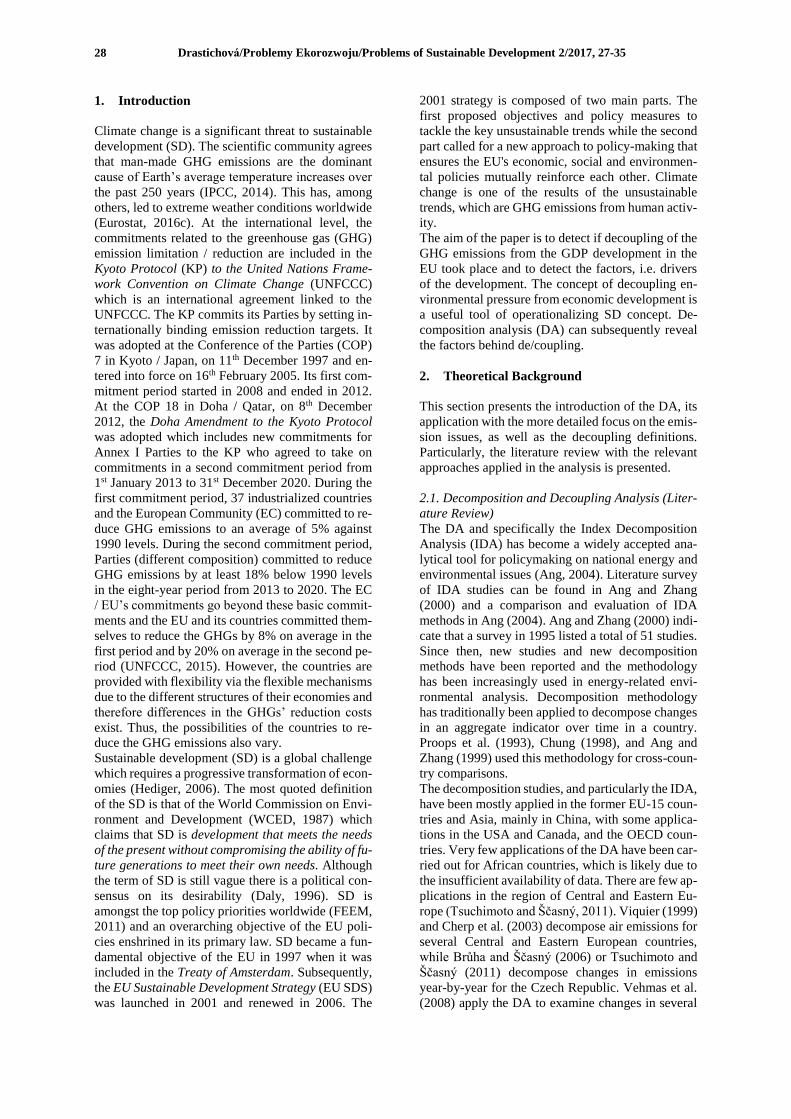
1. Introduction
Climate change is a significant threat to sustainable
development (SD). The scientific community agrees
that man-made GHG emissions are the dominant
cause of Earth’s average temperature increases over
the past 250 years (IPCC, 2014). This has, among
others, led to extreme weather conditions worldwide
(Eurostat, 2016c). At the international level, the
commitments related to the greenhouse gas (GHG)
emission limitation / reduction are included in the
Kyoto Protocol (KP) to the United Nations Frame-
work Convention on Climate Change (UNFCCC)
which is an international agreement linked to the
UNFCCC. The KP commits its Parties by setting in-
ternationally binding emission reduction targets. It
was adopted at the Conference of the Parties (COP)
7 in Kyoto / Japan, on 11th December 1997 and en-
tered into force on 16th February 2005. Its first com-
mitment period started in 2008 and ended in 2012.
At the COP 18 in Doha / Qatar, on 8th December
2012, the Doha Amendment to the Kyoto Protocol
was adopted which includes new commitments for
Annex I Parties to the KP who agreed to take on
commitments in a second commitment period from
1st January 2013 to 31st December 2020. During the
first commitment period, 37 industrialized countries
and the European Community (EC) committed to re-
duce GHG emissions to an average of 5% against
1990 levels. During the second commitment period,
Parties (different composition) committed to reduce
GHG emissions by at least 18% below 1990 levels
in the eight-year period from 2013 to 2020. The EC
/ EU’s commitments go beyond these basic commit-
ments and the EU and its countries committed them-
selves to reduce the GHGs by 8% on average in the
first period and by 20% on average in the second pe-
riod (UNFCCC, 2015). However, the countries are
provided with flexibility via the flexible mechanisms
due to the different structures of their economies and
therefore differences in the GHGs’ reduction costs
exist. Thus, the possibilities of the countries to re-
duce the GHG emissions also vary.
Sustainable development (SD) is a global challenge
which requires a progressive transformation of econ-
omies (Hediger, 2006). The most quoted definition
of the SD is that of the World Commission on Envi-
ronment and Development (WCED, 1987) which
claims that SD is development that meets the needs
of the present without compromising the ability of fu-
ture generations to meet their own needs. Although
the term of SD is still vague there is a political con-
sensus on its desirability (Daly, 1996). SD is
amongst the top policy priorities worldwide (FEEM,
2011) and an overarching objective of the EU poli-
cies enshrined in its primary law. SD became a fun-
damental objective of the EU in 1997 when it was
included in the Treaty of Amsterdam. Subsequently,
the EU Sustainable Development Strategy (EU SDS)
was launched in 2001 and renewed in 2006. The
2001 strategy is composed of two main parts. The
first proposed objectives and policy measures to
tackle the key unsustainable trends while the second
part called for a new approach to policy-making that
ensures the EU's economic, social and environmen-
tal policies mutually reinforce each other. Climate
change is one of the results of the unsustainable
trends, which are GHG emissions from human activ-
ity.
The aim of the paper is to detect if decoupling of the
GHG emissions from the GDP development in the
EU took place and to detect the factors, i.e. drivers
of the development. The concept of decoupling en-
vironmental pressure from economic development is
a useful tool of operationalizing SD concept. De-
composition analysis (DA) can subsequently reveal
the factors behind de/coupling.
2. Theoretical Background
This section presents the introduction of the DA, its
application with the more detailed focus on the emis-
sion issues, as well as the decoupling definitions.
Particularly, the literature review with the relevant
approaches applied in the analysis is presented.
2.1. Decomposition and Decoupling Analysis (Liter-
ature Review)
The DA and specifically the Index Decomposition
Analysis (IDA) has become a widely accepted ana-
lytical tool for policymaking on national energy and
environmental issues (Ang, 2004). Literature survey
of IDA studies can be found in Ang and Zhang
(2000) and a comparison and evaluation of IDA
methods in Ang (2004). Ang and Zhang (2000) indi-
cate that a survey in 1995 listed a total of 51 studies.
Since then, new studies and new decomposition
methods have been reported and the methodology
has been increasingly used in energy-related envi-
ronmental analysis. Decomposition methodology
has traditionally been applied to decompose changes
in an aggregate indicator over time in a country.
Proops et al. (1993), Chung (1998), and Ang and
Zhang (1999) used this methodology for cross-coun-
try comparisons.
The decomposition studies, and particularly the IDA,
have been mostly applied in the former EU-15 coun-
tries and Asia, mainly in China, with some applica-
tions in the USA and Canada, and the OECD coun-
tries. Very few applications of the DA have been car-
ried out for African countries, which is likely due to
the insufficient availability of data. There are few ap-
plications in the region of Central and Eastern Eu-
rope (Tsuchimoto and Ščasný, 2011). Viquier (1999)
and Cherp et al. (2003) decompose air emissions for
several Central and Eastern European countries,
while Brůha and Ščasný (2006) or Tsuchimoto and
Ščasný (2011) decompose changes in emissions
year-by-year for the Czech Republic. Vehmas et al.
(2008) apply the DA to examine changes in several

Drastichová/Problemy Ekorozwoju/Problems of Sustainable Development 2/2017, 27-35
29
indicators. Their analysis is mainly focused on the
indicators in the EU SDIs set and the DA carried out
is based on the Advanced Sustainability Analysis
(ASA) approach and a revised Sun/Shapley decom-
position technique.
Overall, the IDA has also become a useful tool in en-
ergy and environmental analysis in general (Ang and
Zhang, 2000) and as a part of such analysis also one
of the common methods of the emissions trends anal-
ysis (Tsuchimoto and Ščasný, 2011) including CO2
emission topics. As climate change and GHG emis-
sions became a global issue in 1990s, IDA was first
extended from energy consumption to energy-re-
lated CO2 emission studies in 1991. Since then many
studies have been reported for various countries and
emission sectors. Xu and Ang (2013) elaborated a
comprehensive literature survey and revealed the rel-
ative contributions of key effects on changes in the
aggregate carbon intensity by emission sector and by
country. Concerning IDA methodology, decomposi-
tion models for analyzing emission changes are
slightly more complex than those for energy con-
sumption changes. More factors are normally in-
cluded in the IDA identity and a larger dataset is gen-
erally needed. Thus, IDA is a useful analytical tool
for studying the drivers of changes in CO2 emissions.
In energy-related CO2 emission studies, more effects
are included as the aggregate emissions depend on
the fuel mix in energy consumption (Xu and Ang,
2013). Xu and Ang (2013) also concluded that that
energy intensity change was generally the key driver
of changes in the aggregate carbon intensity in most
sectors and countries. In most cases, it contributed to
decreases in the aggregate carbon intensity. If energy
intensity is taken as a proxy for energy efficiency,
improvements in energy efficiency have been the
main driver of decreases in the aggregate carbon in-
tensity for most sectors in most countries. The con-
tribution of activity structure change and that of car-
bon factor change have been less significant. While
there were some uniform patterns among countries
with respect to the underlying developments of the
aggregate carbon intensity, there were also diversi-
ties, which led to differences in development among
countries. This has implications on future develop-
ment of CO2 emissions, especially of the developing
countries. This also indicates that to reduce growth
in future CO2 emissions, countries should focus
more on activity structure and carbon factor. De-
scription and application of the DA to CO2 emissions
in Germany can be found in Seibel (2003).
2.2. Decoupling Definition and Indicators
The aim of the Paper is to detect if decoupling of
GHG emissions from GDP development took place.
The decoupling concept refers to breaking the link
between two variables, often referred to as the driv-
ing force, mainly economic growth expressed in
terms of GDP, and the environmental pressures, such
as the use of natural resources (materials, energy,
land, etc.), the generation of waste, and the emission
of pollutants to air or water, etc. Thus, decoupling
indicates breaking the link between environmental
bads and economic goods (OECD, 2002). It points
out the relative growth rates of a direct pressure on
the environment and of an economically relevant
variable to which it is causally linked. The purpose
of decoupling indicators is to monitor the interde-
pendence between these two different spheres and
they usually measure the decoupling of the environ-
mental pressure from the economic growth over a
given period (OECD, 2003). Decoupling occurs
when the growth rate of the economic driving force
exceeds the growth rate of the environmental pres-
sure over a given period. It can be either absolute or
relative. The first takes place when environmental
variable is stable or decreasing while the economic
one is growing. Decoupling is relative when the en-
vironmental variable is growing, but at a lower rate
than the economic variable (OECD, 2002). Gener-
ally, decoupling is the process that is inevitable to
draw closer and achieve the SD path. Therefore, de-
coupling is also applied in the monitoring of the SD
in the EU using the decoupling indicators
(Drastichová, 2014).
3. Data and Methodology
In this section the source of used data, the indicators
and the applied DA methodology are introduced.
3.1. Data
The used indicators related to the climate change are
included in the Sustainable Development Indicators
(SDIs) set for monitoring of the EU SDS which are
presented in ten themes. They include more than 130
indicators, while ten of them were identified as head-
line indicators (Eurostat, 2016b).
The annual GHG emissions are estimated and re-
ported under the UNFCCC, the KP and the Decision
280/2004/EC. The EU as a party to the UNFCCC re-
ports annually its GHG inventory for the year t-2 and
within the area covered by its Member States. The
inventory also constitutes the EU-15 submission un-
der the KP while the Kyoto basket includes six
gases: carbon dioxide (CO2), methane (CH4), nitrous
oxide (N2O), hydrofluorocarbons (HFCs), perfluoro-
carbons (PFCs), and sulphur hexafluoride (SF6). The
impact of land use, land use changes and forestry
(LULUCF) on the GHG inventories is excluded. In-
ternational aviation is included. Emissions are
weighted according to the global warming potential
of each gas. Emissions in CO2-equivalents are ob-
tained using their global warming potential (GWP)
where the following weighting factors are used:
CO2=1, CH4=21 and N2O=310, SF6=23900. HFCs
and PFCs comprise a large number of different gases
that have different GWPs (Eurostat, 2016c). The
GHG (in CO2 equivalent) indexed to 1990 indicator
shows trends in total man-made emissions of the
Drastichová/Problemy Ekorozwoju/Problems of Sustainable Development 2/2017, 27-35
30
Kyoto basket of GHGs. The indicator does not in-
clude emissions and removals related to LULUCF,
nor does it include emissions from international mar-
itime transport. GHG emissions from international
aviation are included (not included in the data, which
is indexed to the Kyoto base year because these
emissions are not covered by the KP).
The GHG emissions indicators are included in the
EU SDI used for the assessment of the progress to-
wards the objectives and targets of the EU SDS. The
latter indicator, i.e. indexed to 1990, serves as a
headline indicator for the whole Climate Change and
Energy theme and the former, i.e. in million tonnes,
as one of the operational indicators for the Climate
Change subtheme in this theme.
It is important to choose the appropriate GDP indi-
cator for this analysis. As the EU-28 is analysed, data
of Eurostat (Eurostat, 2016a) are used. Firstly, GDP
in chain linked volumes (CLV) (2010), million euro,
and secondly, GDP in current prices, million Pur-
chasing Power Standards (PPS) are used. When PPS
series are used, different price levels between coun-
tries are removed and they should be used for cross-
country comparisons in a specific year but they do
not constitute time series. Chain-linked level series
are created by successively applying previous year's
price's growth rates to the current price figure of a
specific reference year, in this case 2010. On the
other hand, chain-linking involves the loss of addi-
tivity for all years except the reference year and the
directly following year, as these are the only periods
expressed in prices of the reference year. For other
years, chain-linked components of GDP will not sum
to chain-linked GDP, and chain-linked Member
States' GDP will not sum to chain-linked EU GDP.
However, there are no GDP figures, which allow for
comparisons in two dimensions, both time and geo-
graphic area. GDP in CLV PPS to a reference year
should be used to compare countries over time, but
it does not exist (Eurostat, 2014). Thus, both above-
mentioned GDP indicators are applied in the DA to
better estimate the effect of the factors.
As it was explained above, chain-linking involves
the loss of additivity and the sum of EU countries
GDP figures in chain-linked volumes does not ex-
actly equal to the EU-28’s aggregate level. For GDP
in CLV the highest deviation reached 0.199%
(2000). In the case of GDP in PPS, the deviations are
only marginal while the highest reached only 0.012
% (2013). As the EU economy is the subject of the
analysis and its structure is bases on the countries, it
would be difficult to redistribute these deviations
among the countries. However, in percentage terms,
these deviations are relatively low and therefore, the
results of the analysis can still be regarded as relia-
ble.
3.2. Methodology
The DA is aimed at explaining the channels through
which certain factors affect a variable (Tsuchimoto
and Ščasný, 2011). Thus, the different factors need
to be identified whereas this is fully a case-specific
issue (Vehmas et al., 2008). There are two basic
streams of DA, concretely the SDA, which is based
on input-output (IO) models, and the IDA founded
on index theory. While the SDA can distinguish be-
tween a variety of technological and final demand
effects which IDA is not able to detect and can also
capture the indirect effects, i.e. the effect of a direct
change in demand of one sector on the inputs of other
sectors, the IDA merely considers the direct effects,
but requires less data. However, the simplicity and
flexibility of the IDA methodology make it easy to
be adopted in comparison to the SDA where IO ta-
bles are required (Ang, 2004). The starting point of
any DA is to create an equation by means of which
the relations between a dependent variable and sev-
eral underlying causes, i.e. factors, are defined. In
that equation, the product of all the factors has to be
equal to the variable, the change of which is analyzed
in this DA. The selected factors are often the ratios
where the denominator of one factor is equal to the
numerator of the next one. As regards the DA in the
environmental field, the environmentally-related
variable is often decomposed into three factors
which affect its development. The first, scale, or ac-
tivity factor, measures the change in the aggregate
associated with a change in the overall level of the
activity. The second, composition, or structural fac-
tor, is related to changes in the structure of the econ-
omy, i.e. the change in the aggregate linked to the
change in the mix of the activity by sub-category. It
is usually measured via the share of partial, often
sectoral, production in overall production assuming
the constant scale of economy and technologies.
Thirdly, intensity, or technique factor, expresses the
input intensity of a partial / sectoral production, such
as the material, or emission intensity to produce a
unit of an output. More generally, it is the change in
the aggregate associated with changes in the sub-cat-
egory environmental intensities (Tsuchimoto and
Ščasný, 2011).
For the IDA various decomposition methods can be
formulated to quantify the impacts of the factors
changes on the aggregate. The two most important
decomposition approaches are the methods based on
the Divisia Index including the LMDI and those
based on the Laspeyres Index (Ang, 2004). For both
categories, the decomposition can be performed ad-
ditively or multiplicatively and the choice between
the two is arbitrary (Ang, 2004). In multiplicative de-
composition the ratio change of an aggregate, and in
the additive approach its difference change, is de-
composed (Ang, 2004). The differences lie in ease of
result presentation and interpretation (Ang and
Zhang, 2000). For the Divisia index based methods,
Ang and Choi (1997) proposed a refined Divisia
method based on the multiplicative form using a log-
arithmic mean weight function instead of the arith-
metic mean weight function.

Drastichová/Problemy Ekorozwoju/Problems of Sustainable Development 2/2017, 27-35
31
ATable 1. Formulas for Multiplicative and Additive LMDI Decomposition, source: Ščasný and Tsuchimoto (2011), Ang and Zhang
(2000), own elaboration
Multiplicative LMDI Additive LMDI
𝐸𝑡𝑜𝑡𝑎𝑙 =𝐸𝑇
𝐸0 = 𝐸𝑥1 × 𝐸𝑥2 × 𝐸𝑥3𝑥 … × 𝐸𝑥𝑛 (2) ∆𝐸𝑡𝑜𝑡𝑎𝑙 = 𝐸𝑇 − 𝐸0 = ∆𝐸𝑥1 + ∆𝐸𝑥2 + ∆𝐸𝑥3 + ⋯ + ∆𝐸𝑥𝑛 (3)
𝐸𝑡𝑜𝑡𝑎𝑙 =𝐸𝑇
𝐸0 = 𝐸𝑎𝑐𝑡 × 𝐸𝑠𝑡𝑟 × 𝐸𝑖𝑛𝑡 (4) ∆𝐸𝑡𝑜𝑡𝑎𝑙 = 𝐸𝑇 − 𝐸0 = ∆𝐸𝑎𝑐𝑡 + ∆𝐸𝑠𝑡𝑟 + ∆𝐸𝑖𝑛𝑡 (5)
𝐸𝑥𝑘 = 𝑒𝑥𝑝 (∑𝐿(𝐸𝑖
𝑇,𝐸𝑖0)
𝐿(𝐸𝑇,𝐸0)𝑖 𝑥 𝑙𝑛 (𝑥𝑘,𝑖
𝑇
𝑥𝑘,𝑖0 )) (6) 𝐸𝑥𝑘 = ∑ 𝐿(𝐸𝑖
𝑇 , 𝐸𝑖0)𝑖 × 𝑙𝑛 (
𝑥𝑘,𝑖𝑇
𝑥𝑘,𝑖0 ) (7)
Table 2. Description of Variables and Formulas used in the Analysis, source: Ščasný and Tsuchimoto (2011), Ang and Zhang
(2000), author’s elaboration
Formula Indication Description
𝐺𝐻𝐺
= ∑ 𝐺𝐻𝐺𝑖
𝑖
Greenhouse Gas
Emissions
𝐺𝐻𝐺𝑖: GHG emissions in country i; GHG: total GHG emissions in the EU; (in
tonnes, in period t )
∆tGDP; 𝐺𝐷𝑃
= ∑ 𝐺𝐷𝑃
𝑖
Scale effect
The scale (activity) effect: the effect of change in performance of whole economy
on the GHG change, i.e. the effect of the economic growth; 𝐺𝐷𝑃𝑖: GDP in country
i; GDP: overall GDP of the whole EU economy (in period t).
∆t
GDPi
GDP (𝑆𝑖)
Composition ef-
fect
The composition (structural) effect: the effect of changes in countries’ GDP on the
change in GHG emissions levels.
∆𝑡𝐺𝐻𝐺𝑖
𝐺𝐷𝑃𝑖 (𝐼𝑖) Intensity effect
The intensity effect: the effect of changes in GHG emissions intensity across coun-
tries. The GHG intensities in country i in period t: the ratio between the GHG and
the production in GDP terms in the EU countries: 𝐼𝑖 = 𝐺𝐻𝐺𝑖/𝐺𝐷𝑃𝑖.
The logarithmic mean of two positive numbers x and
y is defined as:
𝐿(𝑥, 𝑦) =𝑦−𝑥
𝑙𝑛(𝑦
𝑥)
; 𝐼𝑓 𝑥 ≠ 𝑦, 𝑜𝑡ℎ𝑒𝑟𝑤𝑖𝑠𝑒 𝐿(𝑥, 𝑦) = 𝑥; (1)
From the theoretical foundation viewpoint, the
LMDI I methods seem to be the most appropriate
ones. They comply with basic tests for a good index
number, i.e. the factor-reversal test as well the time-
reversal test. It is a perfect, i.e. no residual decompo-
sition. Multiplicative and additive DA results are
linked by a simple formula. The multiplicative
LMDI I also possesses the additive property in the
log form. Next, the quantitative foundation of the ap-
plied DA using the LMDI is presented by Eq. 2 – 12.
This method is used because it complies with the
property of perfect decomposition, i.e. no residuals
are generated and there is a clear linkage between the
additive and the multiplicative decomposition. The
general formulas are included in Tab. 1. For the mul-
tiplicative LMDI decomposition, the formulas are
presented in the first column, expressed by Eq. 2, 4,
6 and for the additive LMDI in the second column
by Eq. 3, 5, 7. Total environmental effect (Etotal) from
period 0 to period T is generally decomposed into n
factors where Exk denotes the contribution of kth fac-
tor to the change in total environmental effect from
0 to T (Eq. 2 and 3). In terms of three-factor DA Etotal
is divided into an activity effect (Eact), a structural
effect (Estr) and an intensity effect (Eint) (Eq. 4 and
5). Applying the LMDI methodology, the three ef-
fects are calculated from Eq. 6 and 7, using the log-
arithmic weights for the corresponding effects,
where i denotes countries.
Regarding the appropriate properties of the additive
form of LMDI decomposition, it is described in de-
tail. Resulting from Eq. 7, the three effects are calcu-
lated:
∆𝐸𝑎𝑐𝑡 = (∑ 𝐿(𝐸𝑖0; 𝐸𝑖
𝑇)𝑛𝑖=1 ∗ ln (
𝑌𝑇
𝑌0)), (8)
∆𝐸𝑠𝑡𝑟 = (∑ 𝐿(𝐸𝑖0; 𝐸𝑖
𝑇)𝑛𝑖=1 ∗ ln (
𝑆𝑖𝑇
𝑆𝑖0)), (9)
∆𝐸𝑖𝑛𝑡 = (∑ 𝐿(𝐸𝑖0; 𝐸𝑖
𝑇)𝑛𝑖=1 ∗ ln (
𝐼𝑖𝑇
𝐼𝑖0)), (10)
where symbols Y, S, I indicate the scale, structure
and intensity effect respectively and according to the
Eq. 1 we obtain:
𝐿(𝐸𝑖0; 𝐸𝑖
𝑇) = 𝐸𝑖
𝑇−𝐸𝑖0
ln 𝐸𝑖𝑇−ln 𝐸𝑖
0. (11)
Applying the IDA to the relation of GHG emissions
and GDP development, the variables and formulas
are described in Tab. 2. As the analysis is aimed at
the EU and its countries, the structural effect is based
on the structure of the EU, i.e. its countries. This
kind of analysis is crucial to examine the SD path in
the EU, because this methodology is applied to the
issue of decoupling, i.e. the one operationalizing SD,
putting this concept into practise. Moreover, this
analysis is applied to the EU SDIs that are the main
indicators for monitoring the EU SDS. These indica-
tors are organized in a theme-oriented framework
and thus the concrete interlinks among the SD issues
are less visible. So, they can be clearly detected us-
ing the DA.
Using the additive decomposition, the total GHG
emissions in the EU in period t is split into three
components:

Drastichová/Problemy Ekorozwoju/Problems of Sustainable Development 2/2017, 27-35
32
AFigure 1. GHG emissions (in CO2 equivalent) indexed to 1990 (base year = 100) Source: Eurostat (2016c)
Table 3. Results of the year-by-year DA using GDP in CVL (2010) Source: author’s calculations
2001 2002 2003 2004 2005 2006 2007 2008 2009 2010 2011 2012 2013
S
2.221 1.336 1.317 2.529 2.065 3.328 3.053 0.496
-
4.326 2.081 1.720
-
0.475 0.186
C
0.160 0.308 0.442 0.382 0.332 0.438 0.485 0.463 0.191
-
0.066 0.096 0.061 0.080
I
-1.482
-
2.466
-
0.025
-
2.864
-
3.059
-
3.828
-
4.594
-
3.067
-
3.068 0.220
-
4.902
-
1.041
-
2.097
T
0.900
-
0.823 1.734 0.048
-
0.662
-
0.062
-
1.055
-
2.108
-
7.203 2.235
-
3.086
-
1.455
-
1.832
Note: S – scale effect; C - Composition Effect; I – Intensity Effect; T – Total Change (Effect)
∆tGHG = ∑ ∆t𝐺𝐷𝑃 + ∆tGDPi
𝐺𝐷𝑃i +∆t𝐺𝐻𝐺i
GDPi= ∑ 𝑌 + 𝑆𝑖 + 𝐼𝑖 ,𝑛
𝑖=1 (12)
where all the components are described in Tab. 2 (i
– the country, t – the period).
4. Results of Analysis
Firstly, the EU countries’ results of meeting the KP
commitments and subsequently the results of LMDI
decomposition of GHG emissions are presented in
this section.
4.1. The GHG emissions development in the EU
Many of the EU countries achieved significant pro-
gress towards meeting the commitments of the KP in
the first and also in the second period while some
countries have already met the commitments of the
second one (see Fig. 1). Nine transition economies,
except for Cyprus, Malta, Slovenia and Poland,
achieved the GHG emissions reduction by more than
30% in 2013 compared to 1990, while three of them,
i.e. Lithuania, Latvia and Romania, even more than
50%. The emissions increased only in seven coun-
tries including Cyprus and Malta showing the high-
est growth (more than 40%), three Southern coun-
tries, Ireland and Austria. Twelve countries already
achieved the higher reduction than 20% in 2012 and
thirteen in 2013. The EU as a whole showed the re-
duction of 19.85% in 2013 and thus significant pro-
gress has been made towards meeting the Kyoto
commitments.
The development of the GHG emissions can be as-
sessed as quite positive, when significant reduction
1 As it was mentioned in Section 2.1., chain-linking in-
volves the loss of additivity and thus the growth rates of
the aggregate slightly differ from the growth of the sum of
was achieved. The only two cases of significant in-
crease occurred in small island states, Malta and Cy-
prus, both with low level of the overall GHG emis-
sions (3.125 and 9.045 mill. tonnes in 2013 respec-
tively). The transitive economies have had great po-
tential to reduce GHG emissions due to the ineffi-
cient resource use in the former regime and the ma-
jority of them showed the highest drops (Fig. 1). The
countries with the highest total emissions, Germany
and the United Kingdom (604.272 and 976.326 mill.
tonnes in 2013 respectively), also showed significant
drop of emissions compared to 1990. The progress
of other major producers of GHGs, such as France,
Italy, Poland, Spain and Netherlands, was slower.
The varied progress is the result of differences in the
structures of economies, their resource base and a
range of other factors affecting their possibilities to
reduce GHG emissions.
4.2. Decomposition Analysis of GHG emissions in
the EU
The results of the year-by-year DA are presented in
Tab. 3 using GDP in CVL (2010) and in Tab. 4 using
GDP in PPS as indicators of economic activity. Be-
fore the results of the DA are assessed, the annual
changes of GDP and GHG emissions are investi-
gated to detect if decoupling took place. For GDP
this results from the first line of Tab. 3 for GDP in
CLV1 and Tab. 4 for GDP in PPS while the last lines
of these Tables show the GHG emissions changes.
There is only one year in the monitored period with
no decoupling at all, i.e. 2003. The absolute decou-
pling took place in 2002, in every year from 2005 to
the GPDs of the EU countries. However, the direction re-
mains the same and the differences are quite marginal.
41,81
42,96
43,85
80,15100,12 141,29
143,77
020406080
100120140

Drastichová/Problemy Ekorozwoju/Problems of Sustainable Development 2/2017, 27-35
33
A
Table 4. Results of the year-by-year DA using GDP in PPS, source: author’s calculations
2001 2002 2003 2004 2005 2006 2007 2008 2009 2010 2011 2012 2013
S
4.092 3.616 1.620 4.922 4.362 5.611 5.810 0.614
-
5.650 4.350 2.923 1.881 0.846
C 0.114 0.295 0.352 0.350 0.143 0.254 0.390 0.277 0.267 0.188 0.122 0.145 0.032
I
-3.306
-
4.734
-
0.238
-
5,223
-
5.167
-
5.927
-
7.255
-
2.998
-
1.820
-
2.303
-
6.131
-
3.481
-
2.711
T
0.900
-
0.823 1.734 0.048
-
0.662
-
0,062
-
1.055
-
2.108
-
7.203 2.235
-
3.086
-
1.455
-
1.832
Note: S – scale effect; C - Composition Effect; I – Intensity Effect; T – Total Change (Effect)
Figure 2. Results of DA using GDP in CVL (2010) in the overall and two partial periods, source: author’s calculations
2008, in 2011 and 2013. In 2001 and 2004, the rela-
tive decoupling occurred as the GHG emissions an-
nually increased but as slower rate than GDP. In
2009, the most significant effects of the economic
crisis became evident as both GDP and GHG emis-
sions dropped, but the emissions decreased more sig-
nificantly. The results for 2010 and 2012 are not
clear. In 2010, there is no decoupling when GDP in
CLV is used and the relative decoupling when GDP
in PPS is used due to the fact that emissions annually
increased, but the GDP in PPS increased more and
GDP in CLV less than GHG emissions. Emissions
dropped in 2012, similarly GDP in CLV, but at lower
rate. On the other hand, GDP in PPS slightly in-
creased. It is obvious that the results in more recent
period, since 2009, have significantly been affected
by the effects of the economic crisis.
As regards the overall / average change, the scale and
composition effects are positive and the intensity and
total effects are negative for both indicators. The in-
tensity effect followed by the scale effect reached the
highest levels when GDP in PPS is used. For GDP in
CVL these numbers are relatively lower. On the
other hand, the composition effect showed the low-
est absolute value; lower when GDP in PPS is used.
Concerning the annual changes, the scale and com-
position effects are predominantly positive. The
scale effect was only negative in 2009 for both and
in 2012 when GDP in CVL is used. The composition
effect is only negative in 2010 when GDP in CVL is
used and still positive when GDP in PPS is used as
the indicator of economic activity. The intensity ef-
fect is still negative except for 2010 when GDP in
CLV is used. Thus in 2010 the results diverge con-
cerning the direction of the composition and inten-
sity effect. The results correspond with the kind of
decoupling indicated above and those of the more re-
cent period can still be affected by the economic cri-
sis. Although the intensity effect in 2013 helped re-
duce the overall GHG, the scale effect was low due
to the very slow economic growth.
The changes for the overall and two partial periods
are depicted in Fig. 2 and 3. These results confirm
those of the year-by-year DA. The intensity effect
showed the highest extent, but it is negative. This
also affected the total effect, which is negative as
well (except for period 2000-2006), but lower in ab-
solute values, because it is also affected by other two
effects, which were positive in overall as well as in
both partial periods. While the scale effect also
showed the relative higher absolute values, the com-
position effect was only marginal.
Comparing Fig. 2 and 3, it can be seen that the extent
of the scale and intensity effect is relatively higher
when GDP in PPS is used, but the application of this
indicator led to the lower extent of the composition
effect, except for period 2006-2013.
It can be concluded that the intensity effect has
mainly been responsible for the reduction of the
GHG emissions in the EU while the scale effect has
contributed to their increase. However, in the overall
and both partial periods the intensity effect showed
the higher absolute value. The role of composition
effect was only marginal, however, it was positive
and in period 2000–2006, the positive effects out-
weighed the negative intensity effect and the GHG
emissions increased. In the second partial period
2006-2013 and the overall period 2000-2013, the
GHG emissions dropped due to the significant con-
tribution of the negative intensity effect.
This results from the effort of the EU and its coun-
tries to meet the international commitments, particu-
14,361%
3,141%
-30,388%
-12,886%
2,409% 1,258%
-17,516%-13,848%
12,856%
2,090%
-13,830%
1,116%
-32%
-27%
-22%
-17%
-12%
-7%
-2%
3%
8%
13%
Scale Effect Composition Effect Intensity Effect Total Change
13/00 13/06 06/00

Drastichová/Problemy Ekorozwoju/Problems of Sustainable Development 2/2017, 27-35
34
A
Figure 3. Results of DA using GDP in PPS in the overall and two partial periods, source: author’s calculations
larly those of the KP, and of a large number of cor-
responding laws, strategies to reduce GHG emis-
sions, such as the long term EU SDS and Europe
2020 strategy, many initiatives, mitigation and adap-
tation measures. These activities also respond to the
commitments included in the primary law of the EU,
where in the wording of the Lisbon Treaty, Union
policy on the environment shall contribute to the ob-
jectives of promoting measures at international level
to deal with regional or worldwide environmental
problems, and in particular combating climate
change (EU, 2012). The structure of the EU institu-
tions has also been adapted to better meet the objec-
tives related to combating climate change (e.g. estab-
lishment of the Directorate-General for Climate Ac-
tion in the European Commission). The significant
effort to reduce GHG emissions and the impacts of
climate change still needs to be deepened not only in
the EU, but also worldwide, as the effects are still
more visible. Although some flexibility in commit-
ments of the countries is inevitable due to their dif-
ferent conditions, the major producers should take
responsibility and apply appropriate structural re-
forms. As it results from the analysis, the role of the
composition effect in the EU has been marginal. The
EU is composed of the countries with significant dif-
ferences in the overall GHG emissions and success-
ful reduction mainly depends on the major produc-
ers. On the other hand, the international aspects of
this issue should also be considered.
5. Conclusions
The aim of the paper was to detect if decoupling of
the GHG emissions from the GDP development in
the EU took place and to detect the factors of the de-
velopment. The IDA and the LMDI method were ap-
plied to examine the GHG emissions development in
the EU. The EU as a whole showed significant re-
duction of GHG emissions and thus the steady pro-
gress has been made towards meeting the Kyoto
commitments. However, the progress varied among
the countries. This is the result of distinction be-
tween the structures of their economies, their re-
source base and other factors affecting their reduc-
tion possibilities.
In the monitored period 2000-2013 and the second
partial period 2006-2013, the GHG emissions
dropped in the EU due to the significant contribution
of the negative intensity effect. The intensity effect
was mainly responsible for the reduction of the GHG
emissions in the EU while the scale effect contrib-
uted to their increase. The role of composition effect
was only marginal; however, it was positive. In the
overall period 2000-2013 and both partial periods,
the intensity effect showed the higher absolute value.
Only in the first partial period 2000-2006, the posi-
tive scale and composition effects together out-
weighed the negative intensity effect and the GHG
emissions increased. However, this trend was al-
ready reversed. As regards the year-by-year DA, the
results are similar; the major exception is the year
2009 with the negative scale effect caused by the
economic recession. The total change of GHG emis-
sions was negative in the majority of the years and
decoupling took place, often its absolute alternative.
No decoupling was typical only of 2003, but the
more recent years were affected by the economic cri-
sis and the results are ambiguous. The economic
problems, such as the most recent economic crisis,
can significantly affect the results. In 2009, the GDP
as well as GHG emissions dropped while the emis-
sions dropped more significantly. This is not the re-
sult of structural reforms, but economic problems
and recession. While the absolute decoupling oc-
curred in the last monitored year 2013, it was also
not only affected by the negative intensity effect, but
also by very small scale effect.
Thus, the appropriate structural reforms are needed
to further reduce the GHG intensity of the GDP, i.e.
to strengthen the negative intensity effect, which can
lead to the reduction of the GHG emissions also by
stronger economic growth. The EU should continue
in institutional improvements, adopting appropriate
legislation and strategies to combat climate change.
The major producers should intensify their efforts
and the international aspects of the problem should
be taken into account.
32,525%
2,581%
-47,992%
-12,886%
9,857%
1,300%
-25,005%
-13,848%
24,351%
1,515%
-24,749%
1,116%
-48%
-38%
-28%
-18%
-8%
2%
12%
22%
32%
Scale Effect Composition Effect Intensity Effect Total Change
13/00 13/06 06/00

Drastichová/Problemy Ekorozwoju/Problems of Sustainable Development 2/2017, 27-35
35
References
1. ANG B. W., 2004, Decomposition analysis for
policymaking in energy: which is the preferred
method?, in: Energy Policy, vol. 32, no 9,
p.1131-1139.
2. ANG B.W., CHOI K. H., 1997, Decomposition
of Aggregate Energy and Gas Emission
Intensities for Industry: A Refined Divisia Index
Method, in: Energy Journal, vol.18, no 3, p.59-
73.
3. ANG B. W., ZHANG, F. Q., 2000, Survey of
Index Decomposition Analysis in Energy and
Environmental Studies, in: Energy, vol. 25, no
12, p. 1149-1176.
4. ANG B.W., ZHANG F. Q., 1999, Inter-regional
Comparisons of Energy-related CO2 Emissions
using the Decomposition Technique, in:
Energy, vol. 24, no 4, p. 297-305.
5. BRŮHA, J., ŠČASNÝ, M., 2006, Economic
Analysis of Driving Forces of Environmental
Burden during the Transition Process: EKC
hypothesis testing in the Czech Republic. Paper
presented at the 3rd Annual Congress of
Association of Environmental and Resource
Economics (AERE), Kyoto, 4-7 July, 2006.
6. DALY H. E., 1996, Beyond Growth: he
Economics of Sustainable Development,
Beacon Press, Boston.
7. DRASTICHOVÁ M., 2014, Monitoring
Sustainable Development and Decoupling in the
EU, in: Ekonomická revue - Central European
Review of Economic Issues, vol. 17, no 3,
p.125‒140.
8. EU, 2012, Consolidated Version of the Treaty
on the Functioning of the European Union.
Official Journal of the European Union, C
326/132.
9. EUROSTAT, 2016a, Data. Database. Economy
and Finance, http://ec.europa.eu/eurostat/data/
database (10.12.2016).
10. EUROSTAT, 2016b, Sustainable development
indicators. Indicators, http://ec.europa.eu/euro-
stat/web/sdi/indicators (10.12.2016).
11. EUROSTAT, 2016c, Sustainable development
indicators. Indicators. Climate change and
energy, http://ec.europa.eu/eurostat/web/sdi/ind
icators/climate-change-and-energy
(15.12.2016).
12. EUROSTAT, 2014,. Eurostat Metadata.
Annual National Accounts (nama_10) http://
ec.europa.eu/eurostat/cache/metadata/en/nama
_10_esms.htm (16.12.2016).
13. FEEM, 2011, Sustainability Index.
Methodological Report http://www.feemsi.org/
documents/methodological_report2011.pdf
(10.12.2016).
14. HEDIGER W., 2006. Weak and Strong
Sustainability, Environmental Conservation and
Economic Growth, in: Natural Resource
Modeling, vol. 19, no 3, pp. 359-394.
15. CHERP A., KOPTEVA I., MNATSAKANIAN
R., 2003, Economic transition and
environmental sustainability: effects of
economic restructuring on air pollution in the
Russian Federation, in: Journal of Environ-
mental Management, vol. 68, no 2, p.141-151.
16. IPCC, 2014, Summary for policymakers. In:
Climate Change 2014: Impacts, Adaptation,
and Vulnerability. Part A: Global and Sectoral
Aspects. Contribution of Working Group II to
the Fifth Assessment Report of the
Intergovernmental Panel on Climate Change.
Cambridge, United Kingdom and New York,
NY, USA: Cambridge University Press, p. 1-32.
17. OECD, 2002, Sustainable Development. Indi-
cators to measure Decoupling of Environmental
Pressure from Economic Growth. [SG/SD
(2002) 1/FINAL.], OECD, Paris.
18. OECD, 2003, OECD Environmental Indicators.
Development, Measurement and Use [Refe-
rence Paper], OECD, Paris.
19. PROOPS J. L. R., FABER M., WAGENHALS
G., 1993. Reducing CO2 Emissions: a
Comparative Input-Output Study for Germany
and the UK. Springer, Berlin.
20. CHUNG H. S., 1998, Industrial Structure and
Source of Carbon Dioxide Emissions in East
Asia: Estimation and Comparison, in: Energy
and Environment, vol. 9 no 5, p. 509-533.
21. SEIBEL S., 2003, Decomposition analysis of
carbon dioxide-emission changes in Germany -
Conceptual framework and empirical results.
European Communities, Luxembourg.
22. TSUCHIMOTO F., ŠČASNÝ M., 2011,
Decomposition Analysis of Air Pollutant in the
Czech Republic. Paper submitted to 18th
Annual Conference of the European association
of Environmental and Resource Economists
(EAERE), Roma 29 June – 2 July 2011.
23. UNFCCC, 2015, Kyoto Protocol, UN.
24. VEHMAS J., LUUKKANEN J.,
PIHLAJAMÄKI M., 2008, Decomposition
Analysis of EU Sustainable Development
Indicators. Final Report of the DECOIN project
(Development and Comparison of
Sustainability Indicators), Deliverable D3.1 of
WP3, Turku School of Economics, Finland
Futures Research Centre, Turku.
25. VIGUIER L. 1999, Emissions of SO2, NOx and
CO2 in Transition Economies: Emission
Inventories and Divisia index Analysis, in:
Energy Journal, vol. 20, no 2, p.59-87.
26. WCED, 1987, Our common future. Oxford
University Press, Oxford.
27. XU X. Y., ANG B. W., 2013, Index
Decomposition Analysis applied to CO2
Emission Studies, in: Ecological Economics,
vol. 93, p.313-329.

Drastichová/Problemy Ekorozwoju/Problems of Sustainable Development 2/2017, 27-35
36