Decomposition Algorithms with Parametric Gomory Cuts for

Two-Stage Stochastic Integer Programs

Dinakar Gade, Simge Kucukyavuz, Suvrajeet Sen

Integrated Systems Engineering

210 Baker Systems, 1971 Neil Avenue

The Ohio State University, Columbus OH 43210

gade.6,kucukyavuz.2,sen.22@osu.edu

August 15, 2012

Abstract

We consider a class of two-stage stochastic integer programs with binary variables in the first

stage and general integer variables in the second stage. We develop decomposition algorithms

akin to the L-shaped or Benders’ methods by utilizing Gomory cuts to obtain iteratively tighter

approximations of the second-stage integer programs. We show that the proposed methodology

is flexible in that it allows several modes of implementation, all of which lead to finitely con-

vergent algorithms. We illustrate our algorithms using examples from the literature. We report

computational results using the stochastic server location problem instances which suggest that

our decomposition-based approach scales better with increases in the number of scenarios than

a state-of-the art solver which was used to solve the deterministic equivalent formulation.

Keywords: Two-stage stochastic integer programs, Gomory cuts, L-Shaped method, Benders’

decomposition, Lexicographic dual simplex, finite convergence

1 Introduction

The Gomory fractional cutting plane algorithm [16] is one of the earliest cutting plane algorithms

developed to solve pure integer programs. A few years after the introduction of the fractional

cuts, Gomory introduced mixed integer cuts [17] which have been successfully incorporated

into branch-and-bound methods to solve mixed integer programs [4, 8]. Gomory cuts and

their extensions have also been a subject of numerous theoretical studies in the mixed integer

programming area [14, 18, 10]. Similarly, the Benders’ decomposition [5] and L-shaped methods

[38] are amongst the earliest and most successful classes of algorithms for solving stochastic linear

programs and stochastic integer programs with continuous variables in the second stage. Recent

studies [36, 31] extend these algorithms to accommodate binary variables in the second stage.

However, these methods do not accommodate models that require general integer variables in the

This work is supported in part by NSF-CMMI Grant 1100383.

1

second stage. For such instances, the introduction of Gomory cuts would provide significantly

stronger approximations as has been demonstrated for deterministic MILP instances. Despite

the fact that the crux of the methodology (i.e. Gomory cuts, Benders/L-shaped method) has

been in existence for over four decades, the only study that has attempted to integrate these

tools within one algorithm for stochastic integer programs (SIP) is the work of Carøe and Tind

[12]. However, their framework creates first-stage approximations that are very challenging to

optimize. In this paper, we provide a first bridge by devising a finite L-shaped decomposition

algorithm that is driven by parametric Gomory cuts in the second stage. These Gomory cuts

will be parametrized by the first-stage decisions, thus allowing us to adopt a decomposition

framework. This algorithm can be used to solve two-stage stochastic integer programs with

binary first-stage and pure integer second-stage variables. We show that the steps involved in

the algorithm are not only computationally attractive, but also flexible in that they allow several

implementations depending on the requirements of the specific instance under consideration.

Let ω be a random vector defined on a probability space (Ω,F ,P) and let E[·] denote the

usual mathematical expectation operator taken with respect to ω. A standard mathematical

formulation for two-stage SIPs is given in (1)-(7).

min c>x+ E [f(x, ω)] (1)

Ax ≥ b (2)

x ∈ X (3)

where for a particular realization ω of ω, f(x, ω) is defined as

f(x, ω) = min y0 (4)

y0 − g(ω)>y = 0 (5)

W (ω)y = r(ω)− T (ω)x (6)

y ∈ Y. (7)

The sets X ⊆ Rn1+ and Y ⊆ R × Rn2

+ impose discrete, binary or continuous restrictions on the

variables. Here, c ∈ Qn1 , A ∈ Qm1×n1 , b ∈ Qm1 , g(ω) ∈ Qn2 , W (ω) ∈ Qm2(ω)×n2 , T (ω) ∈Qm2(ω)×n1 and r(ω) ∈ Qm2(ω).

Two-stage stochastic programs fall under the large umbrella of optimization problems under

uncertainty. In two-stage stochastic programs with recourse, the decision maker must choose a

vector of current decisions x at a cost c>x under the constraints (2)-(3) before the realization of

the random vector ω. Upon the realization of a particular ω of ω referred to as a scenario, the

decision maker chooses a vector of decisions y in response to the realization ω. The second-stage

decisions incur a cost g(ω)>y under the constraints (6)-(7). The second-stage matrix W (ω) is

referred to as the recourse matrix. The decisions made in the first stage impact the second-stage

constraints through the technology matrix T (ω). We let X := x : (2) − (3) denote the set

of first-stage solutions and Y (x, ω) := y : (5) − (7) denote the set of second-stage feasible

solutions for a given x ∈ X and ω. Typically, the first stage corresponds to strategic or capital

investment decisions and the second stage corresponds to operational decisions made in response

to uncertain events. The most commonly used objective function of two-stage recourse models

is to minimize the first-stage costs and the expected future costs of the second stage. In this

2

paper, we assume that X = x ∈ Bn1 and Y = y ∈ Z× Zn2+ .

Stochastic programs of the type (1)-(7) are amongst the most challenging classes of optimiza-

tion problems. In addition to the usual “curse of dimensionality” due to the multi-dimensional

integral in the expectation calculation of (1), these models have to contend with difficulties

arising from integer recourse problems of the second stage. In order to mitigate some of the

difficulties, we make the following assumptions:

(A1) ω has a finite support on Ω.

(A2) All the data elements in the second stage g(ω),W (ω), r(ω), T (ω) are integral.

(A3) The set X is non-empty.

(A4) Y (x, ω) 6= ∅ for all (x, ω) ∈ X × Ω.

(A5) |E[f(x, ω)]| < +∞.

Because of assumption (A1), the expectation in (1) can be replaced by a weighted sum and one

can write the so-called deterministic equivalent formulation (DEF), which may be viewed as a

large-scale integer program:

min c>x+∑ω∈Ω

pωy0(ω) (8)

Ax ≥ b (9)

y0(ω)− g(ω)>y(ω) = 0, ω ∈ Ω (10)

T (ω)x+W (ω)y(ω) = r(ω), ω ∈ Ω (11)

x ∈ X , y(ω) ∈ Y, ω ∈ Ω, (12)

where P(ω = ω) =: pω. Note that in the decomposed formulation (1)-(7), the dependence of y-

variables on ω is implicit. On the other hand, for the DEF, we express the dependence of y on the

scenario explicitly using ω as an argument since we need to distinguish between the second-stage

solutions for different ω. Throughout the paper, the arguments for y or lack thereof, will be clear

from the context. Assumption (A2) is without loss of generality since the original rational data

can be scaled by a suitable constant to obtain integer coefficients with the same representation.

Assumption (A3) ensures the existence of at least one feasible first-stage solution within a

compact subset of the [0, 1] cube in Rn1 . Assumption (A4) can be enforced for most practical

problems by introducing artificial variables and penalizing the artificial variables in the second-

stage objective. Note that Assumption (A4) implies E[f(x, ω)] <∞. Stochastic programs that

satisfy this assumption are said to possess the relatively complete recourse property. We further

assume in (A5) that the SIP has a finite optimum, i.e., E[f(x, ω)] > −∞ to ensure that the

problem is well defined.

The DEF can be input to an off-the-shelf mixed integer programming (MIP) solver. However,

as is often the case in stochastic programming, one encounters a large number of scenarios which

imposes large memory and computational burden on the solver. One approach to deal with this

difficulty is to work with smaller problems by decomposing the DEF into a first-stage problem

and a collection of second-stage scenario problems. This is possible since for a given x ∈ X,

the scenario problems can be solved independently. Benders’ decomposition or the L-Shaped

method exploit this decomposability and reformulate the problem in the space of the (x, η)-

3

variables as follows:

minx∈Xc>x+ η : η ≥ E[f(x, ω)]. (13)

In an L-shaped algorithm, one constructs sequentially tighter approximations of E[f(x, ω)].

When the second stage is a linear program, f(·, ω) is a convex piecewise linear function and

since E[f(·, ω)] is a convex combination of such functions, it continues to satisfy convexity.

Thus, it is possible to construct approximations of E[f(x, ω)] by using the so-called ‘optimality

cuts’, which are affine. When the second stage is an integer program, f(·, ω) is only lower

semicontinuous and in general non-convex (see Blair and Jeroslow [9], Schultz [28]). Thus,

approximating E[f(x, ω)] becomes a challenge when the second-stage variables are integers.

For SIP problems with pure integer recourse decisions, this paper addresses the following

questions that have remained unresolved to date:

1. Can the expected recourse function E[f(x, ω)] be approximated by piecewise linear func-

tions of the first-stage variables? Such approximations allow the master program to possess

the same structure as in standard Benders’ decomposition, which assumes linear programs

in the second-stage.

2. Is it possible to avoid solving the scenario subproblems to IP optimality in each iteration?

3. Is it possible to design a finitely convergent decomposition algorithm using only cutting

planes to approximate the feasible set of the second-stage?

Our paper resolves these questions with affirmative answers for problems with binary variables

in the first stage and general integer variables in the second stage. As the paper unfolds, we will

discuss the implications of these answers in greater technical depth.

The remainder of the paper is organized as follows: In Section 2, we discuss relevant liter-

ature. In Section 3, we develop a decomposition algorithm driven by parametric Gomory cuts

for the second stage. Section 4 discusses alternative implementations of our main algorithm.

Section 5 deals with the convergence of the algorithms presented in Sections 3 and 4. In Section

6, we illustrate our algorithms using examples from the literature. We report our preliminary

computational experience in Section 7.

2 Literature

For a general introduction to stochastic programming, we refer the reader to Birge and Louveaux

[7] and for surveys on stochastic mixed integer programming (SMIP), to Louveaux and Schultz

[21] and Sen [30]. To aid the discussion of literature, we use a classification scheme to represent

the various classes of two-stage stochastic mixed integer programs. This scheme is based on the

variable restrictions represented by X and Y. We use the sets B,C,D to denote the stages of

the stochastic program that have binary, continuous and discrete variables, respectively. For

example, the class of problems considered in this paper have B = 1, 2, C = ∅, D = 2, i.e.,

binary variables may appear in both stages, no continuous variables may appear in either stage

and general integer variables may appear in the second stage.

Laporte and Louveaux’s [20] L-shaped algorithm was one of the earliest decomposition meth-

ods for SMIPs. Their algorithm solves problems with B = 1, 2, C = 2 and D = 2. They

solve second-stage mixed integer programs to optimality at each iteration and construct first-

stage cuts using the objective function values of the second-stage problems. The potential

4

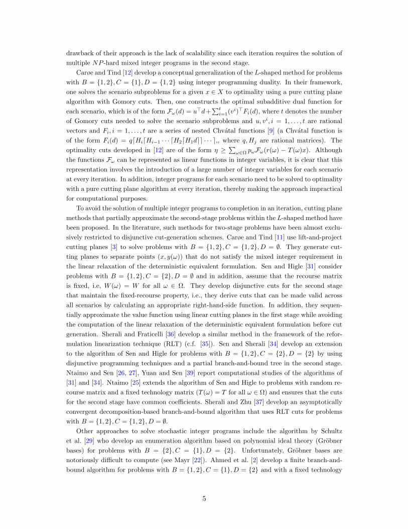
drawback of their approach is the lack of scalability since each iteration requires the solution of

multiple NP -hard mixed integer programs in the second stage.

Carøe and Tind [12] develop a conceptual generalization of the L-shaped method for problems

with B = 1, 2, C = 1, D = 1, 2 using integer programming duality. In their framework,

one solves the scenario subproblems for a given x ∈ X to optimality using a pure cutting plane

algorithm with Gomory cuts. Then, one constructs the optimal subadditive dual function for

each scenario, which is of the form Fω(d) = u>d+∑ti=1(vi)>Fi(d), where t denotes the number

of Gomory cuts needed to solve the scenario subproblems and u, vi, i = 1, . . . , t are rational

vectors and Fi, i = 1, . . . , t are a series of nested Chvatal functions [9] (a Chvatal function is

of the form Fi(d) = qdHidHi−1 · · · dH2dH1dee · · · e,, where q,Hj are rational matrices). The

optimality cuts developed in [12] are of the form η ≥∑ω∈Ω pωFω(r(ω) − T (ω)x). Although

the functions Fω can be represented as linear functions in integer variables, it is clear that this

representation involves the introduction of a large number of integer variables for each scenario

at every iteration. In addition, integer programs for each scenario need to be solved to optimality

with a pure cutting plane algorithm at every iteration, thereby making the approach impractical

for computational purposes.

To avoid the solution of multiple integer programs to completion in an iteration, cutting plane

methods that partially approximate the second-stage problems within the L-shaped method have

been proposed. In the literature, such methods for two-stage problems have been almost exclu-

sively restricted to disjunctive cut-generation schemes. Carøe and Tind [11] use lift-and-project

cutting planes [3] to solve problems with B = 1, 2, C = 1, 2, D = ∅. They generate cut-

ting planes to separate points (x, y(ω)) that do not satisfy the mixed integer requirement in

the linear relaxation of the deterministic equivalent formulation. Sen and Higle [31] consider

problems with B = 1, 2, C = 2, D = ∅ and in addition, assume that the recourse matrix

is fixed, i.e, W (ω) = W for all ω ∈ Ω. They develop disjunctive cuts for the second stage

that maintain the fixed-recourse property, i.e., they derive cuts that can be made valid across

all scenarios by calculating an appropriate right-hand-side function. In addition, they sequen-

tially approximate the value function using linear cutting planes in the first stage while avoiding

the computation of the linear relaxation of the deterministic equivalent formulation before cut

generation. Sherali and Fraticelli [36] develop a similar method in the framework of the refor-

mulation linearization technique (RLT) (c.f. [35]). Sen and Sherali [34] develop an extension

to the algorithm of Sen and Higle for problems with B = 1, 2, C = 2, D = 2 by using

disjunctive programming techniques and a partial branch-and-bound tree in the second stage.

Ntaimo and Sen [26, 27], Yuan and Sen [39] report computational studies of the algorithms of

[31] and [34]. Ntaimo [25] extends the algorithm of Sen and Higle to problems with random re-

course matrix and a fixed technology matrix (T (ω) = T for all ω ∈ Ω) and ensures that the cuts

for the second stage have common coefficients. Sherali and Zhu [37] develop an asymptotically

convergent decomposition-based branch-and-bound algorithm that uses RLT cuts for problems

with B = 1, 2, C = 1, 2, D = ∅.Other approaches to solve stochastic integer programs include the algorithm by Schultz

et al. [29] who develop an enumeration algorithm based on polynomial ideal theory (Grobner

bases) for problems with B = 2, C = 1, D = 2. Unfortunately, Grobner bases are

notoriously difficult to compute (see Mayr [22]). Ahmed et al. [2] develop a finite branch-and-

bound algorithm for problems with B = 1, 2, C = 1, D = 2 and with a fixed technology

5

matrix. Kong et al. [19] study problems with B = 1, 2, C = ∅, D = 1, 2 and in addition

assume that the technology, recourse matrices and the second-stage cost functions are fixed.

Unlike the algorithms discussed in this paragraph, we make no assumptions on the elements of

input data that are affected by the random variables.

Our overall approach is similar to the one taken in [31] in that we iteratively approximate

the second-stage problems using cutting planes. Sen and Higle [31] use disjunctive cuts whereas

we use Gomory cuts within our decomposition algorithm. In Section 6 we compare and contrast

the features of their algorithm with ours using an example.

3 Parametric Gomory Cuts for Decomposition

In this section, we develop a decomposition algorithm driven by Gomory cutting planes to solve

stochastic integer programs. Our approach does not attempt to solve multiple integer scenario

sub-problems in a single iteration but instead, solves only linear programs in the second stage

and generates violated cuts. In order to develop such an approach, we derive valid inequalities of

the form π(ω)>y(ω) ≥ π0(x, ω). Because the right hand side π0 is a function of x, we will refer

to them as parametric Gomory cuts. Toward this end let S(x, ω) := clconv((x, y0(ω), y(ω)) ∈Bn1 × Z× Zn2

+ : y0(ω)− g(ω)>y = 0, T (ω)x+W (ω)y(ω) = r(ω)). Let T c(ω),W c(ω), rc(ω) be

appropriately dimensioned rational matrices so that S(x, ω) = (x, y0(ω), y(ω)) ∈ Rn1+ ×R×R

n2+ :

T c(ω)x + W c(ω)(y0(ω), y(ω)) ≥ rc(ω). Let x denote an extreme point of conv(X). Since the

restriction S(x, ω)∩(x, y0(ω), y(ω)) : x = x yields a face of S(x, ω), the extreme points of the

set Y c(x, ω) := (y0(ω), y(ω)) ∈ R × Rn2+ : W c(ω)(y0(ω), y(ω)) ≥ rc(ω) − T c(ω)x are integral.

We exploit this facial or extreme-point property of binary vectors to derive valid inequalities

π(ω)>y(ω) ≥ π0(x, ω) with π0(·, ω) affine. Affine right hand side functions are clearly desirable

since they are easy to evaluate and they result in first-stage approximations that are piecewise

linear and convex.

In order to derive valid inequalities within a decomposition algorithm, suppose that a binary

first-stage vector x′ is given. Without loss of generality, we can derive the cut coefficients in

a translated space for which the point x′ is the origin. Once the cut coefficients are obtained

in the translated space, it will be straightforward to transform these coefficients to be valid

in the original space. Because x is binary, such translation is equivalent to replacing every

non-zero element xj by its complement, 1− xj . Thus, without loss of generality we will derive

the parametric Gomory cut for a generalized origin x = 0. Let (x, ω) ∈ X × Ω be given and

let B(x, ω) denote an optimal basis of the LP relaxation of the second stage problem. With

this basis, we associate index sets B(x, ω) and N (x, ω) which correspond to basic and nonbasic

variables respectively, and denote N(x, ω) as the submatrix corresponding to non-basic columns.

For ease of exposition, we drop the dependence on (x, ω) and y,B,N,B,N will be in reference

to (x, ω) while T,W, r will be in reference to ω. With a slight abuse of notation, the derivation

here uses x to denote points in the translated space. Multiplying (5)-(6) by B−1 we obtain

yB +B−1NyN = B−1

(0

r − Tx

)=: h(x). (14)

6

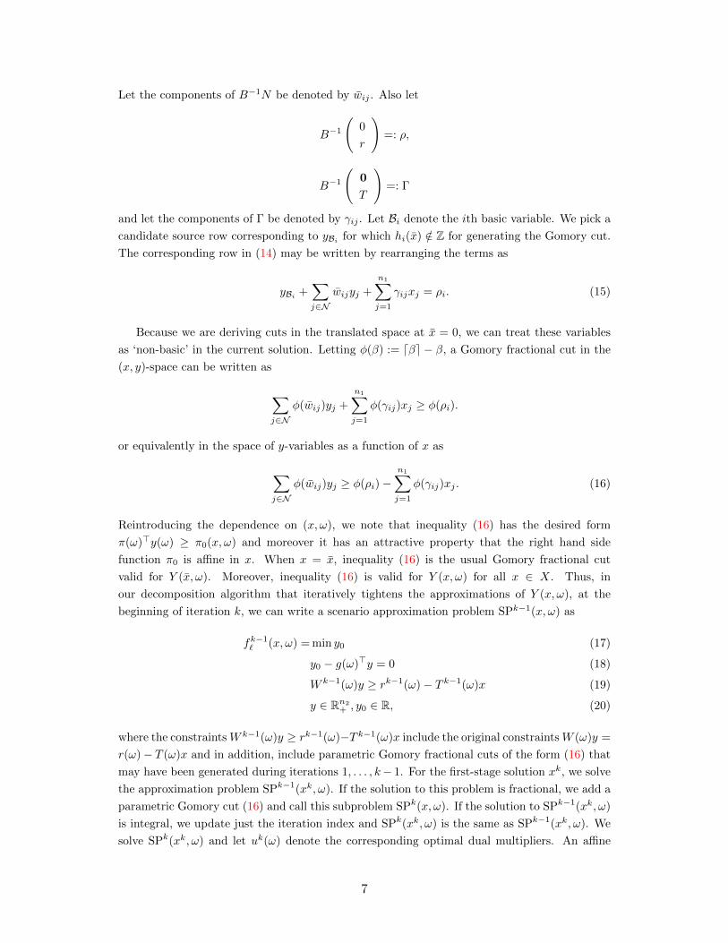
Let the components of B−1N be denoted by wij . Also let

B−1

(0

r

)=: ρ,

B−1

(0

T

)=: Γ

and let the components of Γ be denoted by γij . Let Bi denote the ith basic variable. We pick a

candidate source row corresponding to yBi for which hi(x) /∈ Z for generating the Gomory cut.

The corresponding row in (14) may be written by rearranging the terms as

yBi +∑j∈N

wijyj +

n1∑j=1

γijxj = ρi. (15)

Because we are deriving cuts in the translated space at x = 0, we can treat these variables

as ‘non-basic’ in the current solution. Letting φ(β) := dβe − β, a Gomory fractional cut in the

(x, y)-space can be written as

∑j∈N

φ(wij)yj +

n1∑j=1

φ(γij)xj ≥ φ(ρi).

or equivalently in the space of y-variables as a function of x as

∑j∈N

φ(wij)yj ≥ φ(ρi)−n1∑j=1

φ(γij)xj . (16)

Reintroducing the dependence on (x, ω), we note that inequality (16) has the desired form

π(ω)>y(ω) ≥ π0(x, ω) and moreover it has an attractive property that the right hand side

function π0 is affine in x. When x = x, inequality (16) is the usual Gomory fractional cut

valid for Y (x, ω). Moreover, inequality (16) is valid for Y (x, ω) for all x ∈ X. Thus, in

our decomposition algorithm that iteratively tightens the approximations of Y (x, ω), at the

beginning of iteration k, we can write a scenario approximation problem SPk−1(x, ω) as

fk−1` (x, ω) = min y0 (17)

y0 − g(ω)>y = 0 (18)

W k−1(ω)y ≥ rk−1(ω)− T k−1(ω)x (19)

y ∈ Rn2+ , y0 ∈ R, (20)

where the constraintsW k−1(ω)y ≥ rk−1(ω)−T k−1(ω)x include the original constraintsW (ω)y =

r(ω)− T (ω)x and in addition, include parametric Gomory fractional cuts of the form (16) that

may have been generated during iterations 1, . . . , k− 1. For the first-stage solution xk, we solve

the approximation problem SPk−1(xk, ω). If the solution to this problem is fractional, we add a

parametric Gomory cut (16) and call this subproblem SPk(x, ω). If the solution to SPk−1(xk, ω)

is integral, we update just the iteration index and SPk(xk, ω) is the same as SPk−1(xk, ω). We

solve SPk(xk, ω) and let uk(ω) denote the corresponding optimal dual multipliers. An affine

7

under-estimator of E[f(x, ω)], or an optimality cut can be generated as follows:

η −∑ω∈Ω

pω(uk(ω))>(rk(ω)− T k(ω)x) ≥ 0. (21)

Thus, a lower bounding approximation for (13) at iteration k, denoted by MPk, can be written

as follows:

min c>x+ η (22)

Ax ≥ b (23)

η −∑ω∈Ω

pω(ut(ω))>(rt(ω)− T t(ω)x) ≥ 0, t = 1, . . . , k (24)

x ∈ Bn1 , η ∈ R. (25)

Remark 1. Note that unlike standard Benders’ decomposition, the second-stage LP relaxation

in this algorithm is updated from one iteration to the next, and moreover, these approximations

include affine functions of first-stage variables. These lifted cuts are then used to obtain affine

approximations of second-stage (IP) value functions. In this sense, for the class of problems

studied here, the lifting allows us to overcome complicated sub-additive functions as proposed

by Carøe and Tind [12].

Remark 2. The reader might recall that for mixed binary second-stage recourse problems, Sen

and Higle [31] present a similar algorithm using disjunctive cuts. However, those cuts give rise

to piecewise linear concave functions for π0(x, ω) and as a result require further convexification

for use within a Benders’ type method.

Before stating the decomposition algorithm, we introduce the following additional notation.

An iteration of the algorithm is denoted by k and LBk, UBk denote the lower and upper bounds

on the optimal objective function value of SIP at iteration k. A decomposition algorithm with

parametric Gomory cuts in the second stage is given in Algorithm 1.

The algorithm executes as follows: We initialize the master problem with no optimality cuts,

and subproblems using their linear relaxations. We start with some x1 ∈ X. In iteration k,

using the first-stage solution xk, we solve the scenario approximation problems SPk−1(xk, ω) for

each ω ∈ Ω. If the second-stage solutions for each scenario are integral, it implies that we have

found a feasible solution and we update the best upper bound UBk+1. On the other hand, for

each scenario ω for which the solution y(ω) is non-integral, we generate a Gomory cut (16) from

the smallest index row whose right hand side is fractional. With the cut added to the current

approximation, we obtain the matrices W k(ω), T k(ω), rk(ω). We solve the resulting problem

SPk(xk, ω) using the lexicographic dual simplex method and update the best upper bound if

integer solutions are obtained for SPk(xk, ω) for all ω ∈ Ω. If no cut is generated for a scenario ω,

the matrices W k(ω), T k(ω), rk(ω) are set to W k−1(ω), T k−1(ω), rk−1(ω), respectively. We then

construct an optimality cut (21) using the optimal dual multipliers of the SPk(xk, ω). We solve

the updated master problem MPk using branch-and-bound, to obtain a first-stage solution xk+1

and a lower bound LBk+1 for the SIP and increment the iteration index. We repeat this process

until the stopping condition, UBk = LBk is met. In a computer implementation, alternate

stopping criteria can be used, for example, for a pre-specified tolerance ε, we can terminate the

algorithm when UBk − LBk < ε.

8

Algorithm 1 Decomposition with Parametric Gomory Cuts for 2-Stage SIP

1: Initialization: k ← 1, LB1 ← −∞, UB1 ← +∞, W 0(ω) ← W (ω), T 0(ω) ← T (ω), r0(ω) ←r(ω). Let x1 ∈ X.

2: while LBk < UBk do3: Solve SPk−1(xk, ω) for all ω ∈ Ω using the lexicographic dual simplex method.4: if the solution to SPk−1(xk, ω), y(ω) ∈ Z× Zn2 for all ω ∈ Ω then5: Put W k(ω)←W k−1(ω), T k(ω)← T k−1(ω), rk(ω)← rk−1(ω).6: Update UBk+1 ← min(UBk, c>xk +

∑ω∈Ω pωf

k` (xk, ω)).

7: else8: For all ω ∈ Ω s.t. Ik(ω) := i ∈ 0, . . . , n2 : yi(ω) /∈ Z 6= ∅, choose the source row

corresponding to the smallest index i ∈ Ik(ω) and generate Gomory fractional cut (16).Add the cut to SPk−1(x, ω) to get W k(ω), T k(ω), rk(ω). Put W k(ω)←W k−1(ω), T k(ω)←T k−1(ω), rk(ω)← rk−1(ω) for all ω with Ik(ω) = ∅.

9: Solve SPk(xk, ω) for all ω with Ik(ω) 6= ∅ using the lexicographic dual simplex method.10: If the solution to SPk(xk, ω), y(ω) ∈ Z × Zn2 , update UBk+1 ← min(UBk, c>xk +∑

ω∈Ω pωfk` (xk, ω)).

11: end if12: Add optimality cut (21) to MPk and solve MPk.13: Set xk+1, LBk+1 to the optimal first-stage solution and objective of MPk, respectively.14: k ← k + 1.15: end while16: return xk, c>xk +

∑ω∈Ω pωf

k` (xk, ω).

We conclude this section by noting that Algorithm 1 is also applicable when continuous and

general integer variables are present in the first stage, but their coefficients in the technology

matrix are zeros.

4 Alternative Implementations

In this section, we develop the following alternative implementations of Algorithm 1.

1. Multiple cuts in the first stage (multicut implementation)

2. A round of cuts in the second stage

3. Parametric Gomory mixed integer cuts in the second stage

4. Fixed recourse matrix

5. Partial branch-and-cut for binary second stage.

The first two implementations are relatively straightforward, while the last three require greater

discussion and are described in subsections 4.1-4.3.

The multicut version [6] of this algorithm approximates the value function f(x, ω) for each

ω ∈ Ω by adding |Ω| optimality cuts in the first stage. Disaggregated cuts in the first stage may

reduce the number of main iterations performed since more information is passed on to the first

stage. A potential drawback is that if there are many scenarios, the large number of first-stage

cuts may slow down the solution of the master problems.

An alternative implementation of our algorithm incorporates multiple violated Gomory cuts

in the second stage per iteration, potentially as many as the number of fractional variables for

each scenario. This approach of adding cutting planes from all rows corresponding to fractional

9

variables is referred to as adding a round of cuts. In the mixed integer programming literature,

a number of authors demonstrate the computational superiority of adding a round of cuts over

adding a single cut in each iteration (see for example [4]).

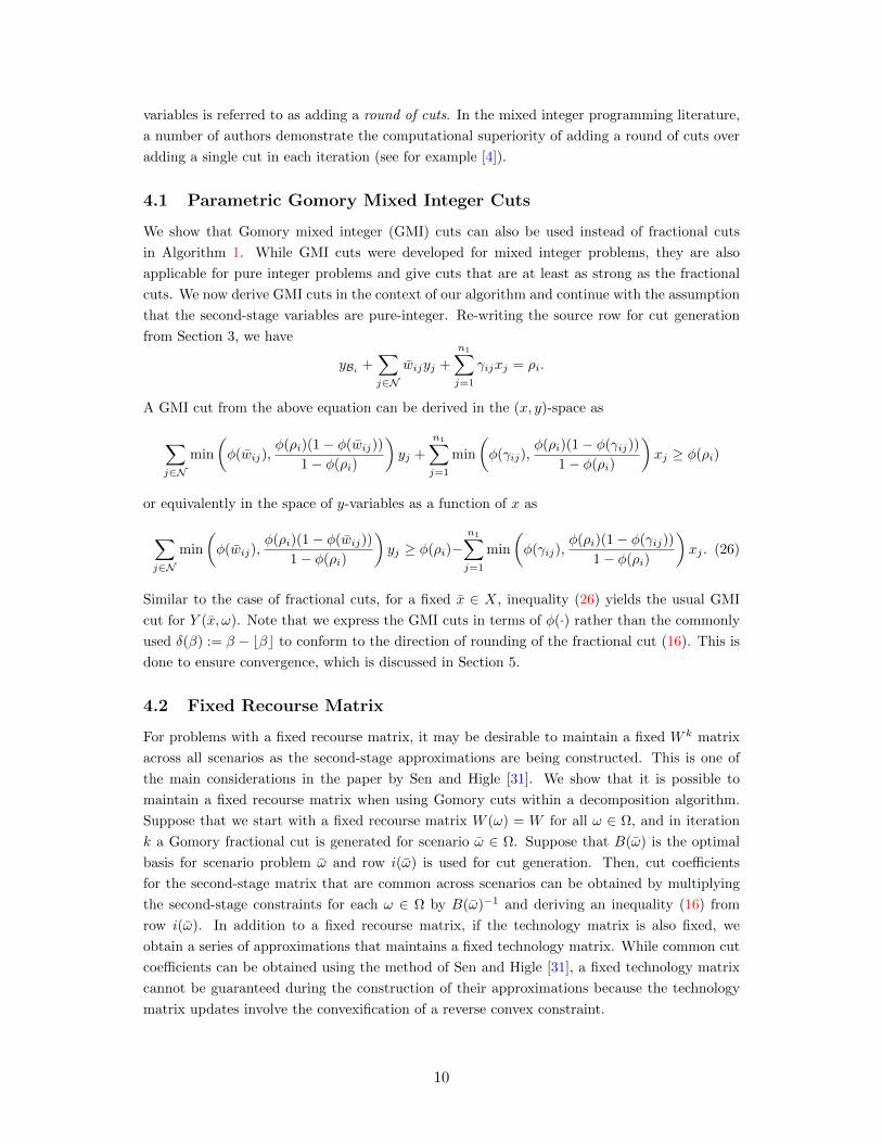
4.1 Parametric Gomory Mixed Integer Cuts

We show that Gomory mixed integer (GMI) cuts can also be used instead of fractional cuts

in Algorithm 1. While GMI cuts were developed for mixed integer problems, they are also

applicable for pure integer problems and give cuts that are at least as strong as the fractional

cuts. We now derive GMI cuts in the context of our algorithm and continue with the assumption

that the second-stage variables are pure-integer. Re-writing the source row for cut generation

from Section 3, we have

yBi+∑j∈N

wijyj +

n1∑j=1

γijxj = ρi.

A GMI cut from the above equation can be derived in the (x, y)-space as

∑j∈N

min

(φ(wij),

φ(ρi)(1− φ(wij))

1− φ(ρi)

)yj +

n1∑j=1

min

(φ(γij),

φ(ρi)(1− φ(γij))

1− φ(ρi)

)xj ≥ φ(ρi)

or equivalently in the space of y-variables as a function of x as

∑j∈N

min

(φ(wij),

φ(ρi)(1− φ(wij))

1− φ(ρi)

)yj ≥ φ(ρi)−

n1∑j=1

min

(φ(γij),

φ(ρi)(1− φ(γij))

1− φ(ρi)

)xj . (26)

Similar to the case of fractional cuts, for a fixed x ∈ X, inequality (26) yields the usual GMI

cut for Y (x, ω). Note that we express the GMI cuts in terms of φ(·) rather than the commonly

used δ(β) := β − bβc to conform to the direction of rounding of the fractional cut (16). This is

done to ensure convergence, which is discussed in Section 5.

4.2 Fixed Recourse Matrix

For problems with a fixed recourse matrix, it may be desirable to maintain a fixed W k matrix

across all scenarios as the second-stage approximations are being constructed. This is one of

the main considerations in the paper by Sen and Higle [31]. We show that it is possible to

maintain a fixed recourse matrix when using Gomory cuts within a decomposition algorithm.

Suppose that we start with a fixed recourse matrix W (ω) = W for all ω ∈ Ω, and in iteration

k a Gomory fractional cut is generated for scenario ω ∈ Ω. Suppose that B(ω) is the optimal

basis for scenario problem ω and row i(ω) is used for cut generation. Then, cut coefficients

for the second-stage matrix that are common across scenarios can be obtained by multiplying

the second-stage constraints for each ω ∈ Ω by B(ω)−1 and deriving an inequality (16) from

row i(ω). In addition to a fixed recourse matrix, if the technology matrix is also fixed, we

obtain a series of approximations that maintains a fixed technology matrix. While common cut

coefficients can be obtained using the method of Sen and Higle [31], a fixed technology matrix

cannot be guaranteed during the construction of their approximations because the technology

matrix updates involve the convexification of a reverse convex constraint.

10

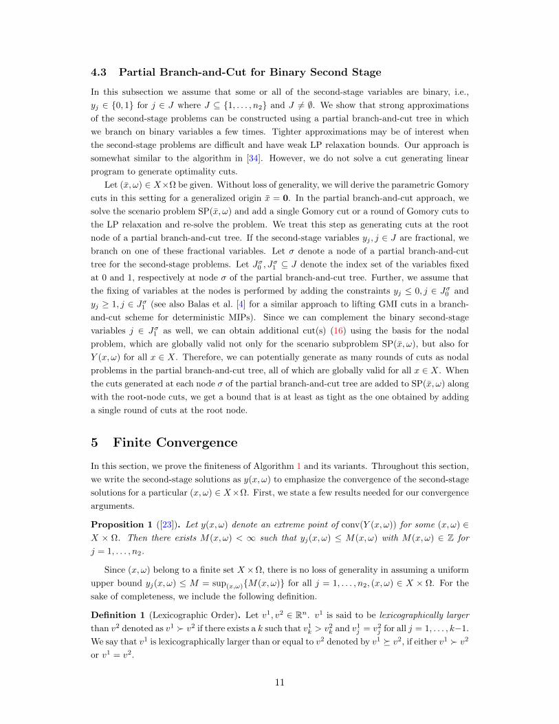
4.3 Partial Branch-and-Cut for Binary Second Stage

In this subsection we assume that some or all of the second-stage variables are binary, i.e.,

yj ∈ 0, 1 for j ∈ J where J ⊆ 1, . . . , n2 and J 6= ∅. We show that strong approximations

of the second-stage problems can be constructed using a partial branch-and-cut tree in which

we branch on binary variables a few times. Tighter approximations may be of interest when

the second-stage problems are difficult and have weak LP relaxation bounds. Our approach is

somewhat similar to the algorithm in [34]. However, we do not solve a cut generating linear

program to generate optimality cuts.

Let (x, ω) ∈ X×Ω be given. Without loss of generality, we will derive the parametric Gomory

cuts in this setting for a generalized origin x = 0. In the partial branch-and-cut approach, we

solve the scenario problem SP(x, ω) and add a single Gomory cut or a round of Gomory cuts to

the LP relaxation and re-solve the problem. We treat this step as generating cuts at the root

node of a partial branch-and-cut tree. If the second-stage variables yj , j ∈ J are fractional, we

branch on one of these fractional variables. Let σ denote a node of a partial branch-and-cut

tree for the second-stage problems. Let Jσ0 , Jσ1 ⊆ J denote the index set of the variables fixed

at 0 and 1, respectively at node σ of the partial branch-and-cut tree. Further, we assume that

the fixing of variables at the nodes is performed by adding the constraints yj ≤ 0, j ∈ Jσ0 and

yj ≥ 1, j ∈ Jσ1 (see also Balas et al. [4] for a similar approach to lifting GMI cuts in a branch-

and-cut scheme for deterministic MIPs). Since we can complement the binary second-stage

variables j ∈ Jσ1 as well, we can obtain additional cut(s) (16) using the basis for the nodal

problem, which are globally valid not only for the scenario subproblem SP(x, ω), but also for

Y (x, ω) for all x ∈ X. Therefore, we can potentially generate as many rounds of cuts as nodal

problems in the partial branch-and-cut tree, all of which are globally valid for all x ∈ X. When

the cuts generated at each node σ of the partial branch-and-cut tree are added to SP(x, ω) along

with the root-node cuts, we get a bound that is at least as tight as the one obtained by adding

a single round of cuts at the root node.

5 Finite Convergence

In this section, we prove the finiteness of Algorithm 1 and its variants. Throughout this section,

we write the second-stage solutions as y(x, ω) to emphasize the convergence of the second-stage

solutions for a particular (x, ω) ∈ X×Ω. First, we state a few results needed for our convergence

arguments.

Proposition 1 ([23]). Let y(x, ω) denote an extreme point of conv(Y (x, ω)) for some (x, ω) ∈X × Ω. Then there exists M(x, ω) < ∞ such that yj(x, ω) ≤ M(x, ω) with M(x, ω) ∈ Z for

j = 1, . . . , n2.

Since (x, ω) belong to a finite set X ×Ω, there is no loss of generality in assuming a uniform

upper bound yj(x, ω) ≤ M = sup(x,ω)M(x, ω) for all j = 1, . . . , n2, (x, ω) ∈ X × Ω. For the

sake of completeness, we include the following definition.

Definition 1 (Lexicographic Order). Let v1, v2 ∈ Rn. v1 is said to be lexicographically larger

than v2 denoted as v1 v2 if there exists a k such that v1k > v2

k and v1j = v2

j for all j = 1, . . . , k−1.

We say that v1 is lexicographically larger than or equal to v2 denoted by v1 v2, if either v1 v2

or v1 = v2.

11

Let β− := min(β, 0) and β+ := max(0, β). From Proposition 1, it follows that if y(x, ω) ∈Y (x, ω) for (x, ω) ∈ X × Ω, then n2∑

j=1

gj(ω)+M,M, . . . ,M

> y(x, ω)

n2∑j=1

gj(ω)−M, 0, . . . , 0

> . (27)

The proof of convergence of Gomory’s fractional cutting plane algorithm relies on the lexi-

cographic dual simplex method [24, 23]. In this version of the simplex method, one begins with

and maintains simplex tableaus that are lexicographically dual feasible, i.e., tableaus that are

dual feasible and have all the nonbasic columns lexicographically smaller than zero. This is

accomplished by using a lexicographic pivoting rule. This approach ensures that the simplex

method does not cycle, and furthermore, guarantees that the lexicographically smallest optimal

solution to the linear program, if it exists, is found in finitely many steps.

The following is a key result that establishes a rounding property of the Gomory fractional

cutting plane algorithm and is used to prove the finiteness of Gomory’s fractional cutting plane

algorithm.

Proposition 2 ([24]). Let (x, ω) ∈ X × Ω be given. Let yt(x, ω) denote the lexicographically

smallest optimal solution to SPt(x, ω), t = k− 1, k, where the updated subproblem SPk is formed

by adding a Gomory cut (16) corresponding to the smallest index source row of the fractional

solution yk−1(x, ω). Let ik denote the index of the variable used to form the Gomory cut, and

define

αk(x, ω) :=(yk−1

0 (x, ω), yk−11 (x, ω), . . . , yk−1

ik−1(x, ω), dyk−1ik

(x, ω)e, 0, . . . , 0)>. (28)

Then,

yk(x, ω) αk(x, ω) yk−1(x, ω).

The following result shows that for a given x ∈ X, we obtain a lexicographically increasing

sequence of αk(x, ω)’s.

Lemma 1. Let (x, ω) ∈ X × Ω be given and let t, k denote two iterations such that t > k, and

xk = xt = x and yj(x, ω) are non-integral for j = k, t. Then αt(x, ω) αk(x, ω).

Proof. It is sufficient to prove the result for the case in which t denotes the first iteration

following k for which xt = xk = x. For xk = x, we have

yk(xk, ω) αk(xk, ω),

using Proposition 2. Since the inequalities added during iterations k + 1, . . . , t − 1 are valid

for Y (x, ω) for all x ∈ X and yj(x, ω) is the lexicographically smallest optimal solution for

SPj(x, ω), j = k, t− 1, we have for xt = x

yt−1(xt, ω) yk(xk, ω).

Furthermore, from (28) we have

αt(xt, ω) yt−1(xt, ω),

12

and the result follows.

The next result shows that in the worst case, Algorithm 1 finds integral solutions to the

second-stage problems for a given (x, ω) ∈ X × Ω. In the following, if no cuts are generated at

iteration k for scenario ω, yk−1(xk, ω) and yk(xk, ω) will denote the same vector.

Lemma 2. Let (x, ω) ∈ X×Ω be given. Then there exists an integer K(x, ω), 0 < K(x, ω) <∞such that either the algorithm terminates in k < K(x, ω) iterations or yk(x, ω) ∈ Z × Zn2

+ and

fk` (x, ω) = f(x, ω) for all k ≥ K(x, ω).

Proof. Let K(x, ω) := k1, k2, . . . , ks, . . . denote a set of increasing iteration numbers such that

k ∈ K(x, ω) if and only if xk = x. From Lemma 1, it follows that if yki−1(xki , ω), ki ∈ K(x, ω)

is fractional, then,

αk1(xk1 , ω) ≺ αk2(xk2 , ω) ≺ · · · ≺ αks(xks , ω) ≺ · · · .

Furthermore, from Proposition 2, we have yk(xk, ω) αk(xk, ω) for all k. Since there are only

finitely many y(x, ω) that satisfy (27), this implies that in the worst case, we obtain an integer

optimal solution to SPk(x, ω) at some k = K(x, ω) ∈ K(x, ω). Finally, since the cuts generated

for x ∈ X such that x 6= x during iterations k /∈ K(x, ω) are also valid for Y (x, ω), in any

iteration k ≥ K(x, ω), we also have yk(x, ω) ∈ Z× Zn2+ and fk` (x, ω) = f(x, ω).

The next result shows that Algorithm 1 is finite.

Theorem 1. Suppose that Assumptions (A1)-(A5) are satisfied. Then, Algorithm 1 finds an

optimal solution to (1)-(7) with X = x ∈ Bn1 and Y = y ∈ Z × Zn2+ in finitely many

iterations.

Proof. Let K = sup(x,ω)∈X×ΩK(x, ω), where K(x, ω) is defined in Lemma 2. Since there are

finitely many (x, ω) ∈ X × Ω, Lemma 2 implies that K <∞. It follows that in the worst case,

for k ≥ K, we obtain yk(xk, ω) ∈ Z × Zn2+ and fk` (xk, ω) = f(xk, ω), for all ω ∈ Ω and no

second-stage cuts are generated after iteration k > K. Then, the convergence of Algorithm 1

follows from the convergence of the Benders’ or L-shaped methods.

Corollary 1. Suppose that Assumptions (A1)-(A5) are satisfied.

(a) The multicut, round-of-cuts, and the Gomory mixed integer-cut implementations find an

optimal solution to (1)-(7) with X = x ∈ Bn1 and Y = y ∈ Z × Zn2+ in finitely many

iterations.

(b) Suppose that we begin with a fixed recourse matrix W (ω) = W for all ω ∈ Ω. Then the fixed

recourse matrix implementation finds an optimal solution to (1)-(7) with X = x ∈ Bn1and Y = y ∈ Z× Zn2

+ in finitely many iterations.

(c) The branch-and-cut implementation finds an optimal solution to (1)-(7) with X = x ∈Bn1 and Y = y ∈ Z× Zn2

+ , 0 ≤ yj ≤ 1, j ∈ J, where J ⊆ 1, . . . , n2, J 6= ∅, in finitely

many iterations.

Proof. The convergence of all the alternative implementations follows automatically from the

arguments given in Lemmas 1 and 2. Indeed, this is obvious for the multicut implementation. For

the round-of-cuts and the partial branch-and-cut implementations, since all the cuts including

13

the one generated from the first fractional source row are present, these results hold. For the

Gomory mixed integer cut implementation, it can be shown that Proposition 2 holds (c.f. [17])

and as a result, Lemmas 1 and 2 hold for this case as well. For the fixed recourse matrix

implementation, although only one scenario is used to derive the common cuts, note that in the

worst case, Gomory cuts for each scenario will be generated eventually. Thus, Lemma 1 holds

and convergence follows.

Several remarks are in order.

Remark 3. Note that in Line 3 of the algorithm, the lexicographic dual simplex method only

ensures the convergence of the simplex method. However, the lexicographic dual simplex method

in Line 9 is crucial to ensure the rounding property of Proposition 2 when Gomory cuts are added

to the LP subproblems and re-optimized.

Remark 4. A number of finite cutting plane algorithms for deterministic MIP problems rely

on ‘memory’ to prove finiteness. For example, in the case of disjunctive cutting plane methods

for MIPs, one maintains a memory of row indices for binary MIPs [33, 3] or a tree for general

bounded MIPs [13] to obtain sequential convexification. These ideas are carried over to the

SMIP case to show convergence of the decomposition algorithms based on disjunctive methods

[31]. On the other hand, in Gomory’s algorithm one can implicitly associate a lexicographic

enumeration tree [23] that automatically provides this memory. For the SIP case, we can

associate a lexicographic enumeration tree for each Y (x, ω) where (x, ω) ∈ X × Ω. Although

a particular x ∈ X may reappear only after a few iterations, Lemma 1 shows that the trees

corresponding to Y (x, ω), ω ∈ Ω are preserved and they get pruned whenever cuts are generated

for these sets. In this sense, Lemma 1 offers a broader characterization of convergence of

algorithms that use Gomory cuts.

Remark 5. In the algorithms for SMIPs based on the disjunctive decomposition schemes, higher

dimensional cut generating linear programs (CGLPs), which themselves have the structure of

two-stage stochastic linear programs, are solved to obtain cuts and the right-hand sides functions.

On the other hand, the parametric Gomory cuts developed in our framework can be obtained

by relatively simple operations. Indeed, the computationally expensive tasks for computing cuts

in our algorithm involve lexicographic pivoting and computing Γ(ω) and ρ(ω). Zanette et al.

[40] suggest guidelines for the implementation of a method that obtains the lexicographically

smallest solution without performing lexicographic pivots.

6 Examples from the Literature

In this section we illustrate Algorithm 1 using examples from the literature. Our goal here

is to illustrate the algorithm via a prototype and exclude any extraneous features. Therefore,

we first implement Algorithm 1 in MATLAB (version 2011b). Our implementation includes a

full-tableau lexicographic dual simplex method to solve the subproblems. We solve the master

problems using pure branch-and-bound with CPLEX. The second-stage cuts are derived from a

source row as Chvatal cuts [14], which are equivalent to the fractional cuts and ensure integer cut

coefficients. Consider the following example that appears in Sen et al. [32], which is a variation

of an example from Schultz et al. [29].

14

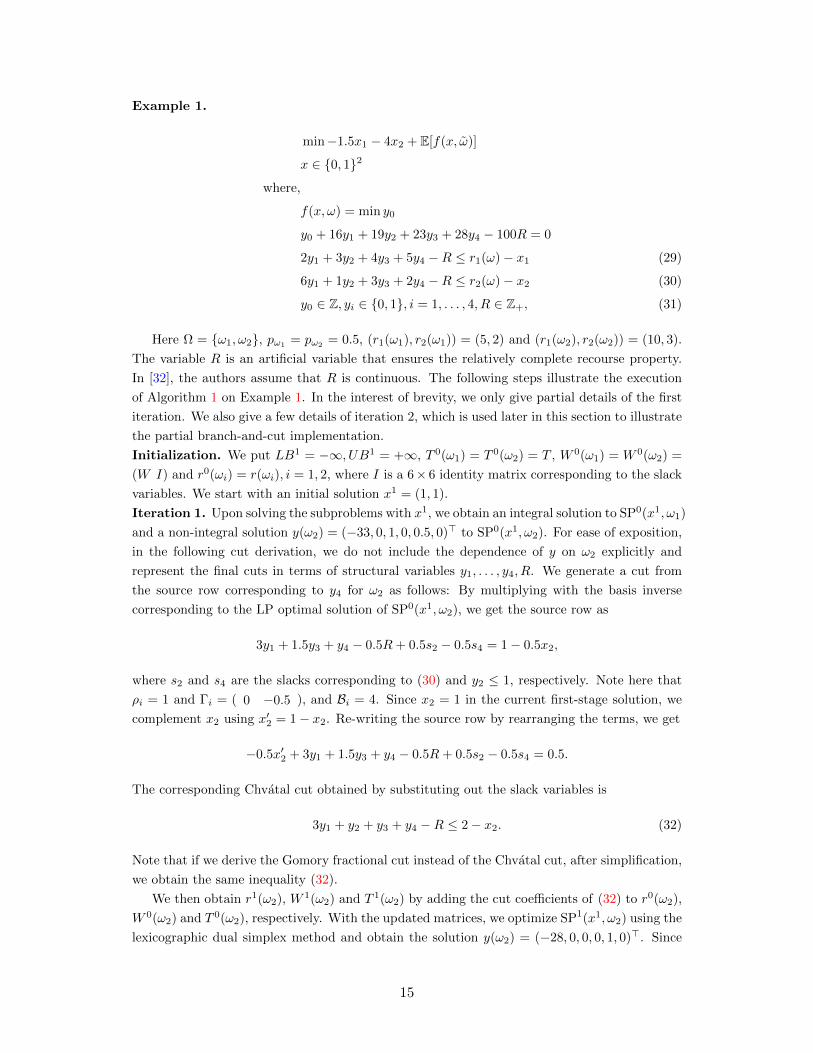
Example 1.

min−1.5x1 − 4x2 + E[f(x, ω)]

x ∈ 0, 12

where,

f(x, ω) = min y0

y0 + 16y1 + 19y2 + 23y3 + 28y4 − 100R = 0

2y1 + 3y2 + 4y3 + 5y4 −R ≤ r1(ω)− x1 (29)

6y1 + 1y2 + 3y3 + 2y4 −R ≤ r2(ω)− x2 (30)

y0 ∈ Z, yi ∈ 0, 1, i = 1, . . . , 4, R ∈ Z+, (31)

Here Ω = ω1, ω2, pω1= pω2

= 0.5, (r1(ω1), r2(ω1)) = (5, 2) and (r1(ω2), r2(ω2)) = (10, 3).

The variable R is an artificial variable that ensures the relatively complete recourse property.

In [32], the authors assume that R is continuous. The following steps illustrate the execution

of Algorithm 1 on Example 1. In the interest of brevity, we only give partial details of the first

iteration. We also give a few details of iteration 2, which is used later in this section to illustrate

the partial branch-and-cut implementation.

Initialization. We put LB1 = −∞, UB1 = +∞, T 0(ω1) = T 0(ω2) = T , W 0(ω1) = W 0(ω2) =

(W I) and r0(ωi) = r(ωi), i = 1, 2, where I is a 6× 6 identity matrix corresponding to the slack

variables. We start with an initial solution x1 = (1, 1).

Iteration 1. Upon solving the subproblems with x1, we obtain an integral solution to SP0(x1, ω1)

and a non-integral solution y(ω2) = (−33, 0, 1, 0, 0.5, 0)> to SP0(x1, ω2). For ease of exposition,

in the following cut derivation, we do not include the dependence of y on ω2 explicitly and

represent the final cuts in terms of structural variables y1, . . . , y4, R. We generate a cut from

the source row corresponding to y4 for ω2 as follows: By multiplying with the basis inverse

corresponding to the LP optimal solution of SP0(x1, ω2), we get the source row as

3y1 + 1.5y3 + y4 − 0.5R+ 0.5s2 − 0.5s4 = 1− 0.5x2,

where s2 and s4 are the slacks corresponding to (30) and y2 ≤ 1, respectively. Note here that

ρi = 1 and Γi = ( 0 −0.5 ), and Bi = 4. Since x2 = 1 in the current first-stage solution, we

complement x2 using x′2 = 1− x2. Re-writing the source row by rearranging the terms, we get

−0.5x′2 + 3y1 + 1.5y3 + y4 − 0.5R+ 0.5s2 − 0.5s4 = 0.5.

The corresponding Chvatal cut obtained by substituting out the slack variables is

3y1 + y2 + y3 + y4 −R ≤ 2− x2. (32)

Note that if we derive the Gomory fractional cut instead of the Chvatal cut, after simplification,

we obtain the same inequality (32).

We then obtain r1(ω2), W 1(ω2) and T 1(ω2) by adding the cut coefficients of (32) to r0(ω2),

W 0(ω2) and T 0(ω2), respectively. With the updated matrices, we optimize SP1(x1, ω2) using the

lexicographic dual simplex method and obtain the solution y(ω2) = (−28, 0, 0, 0, 1, 0)>. Since

15

Table 1: Decomposition with Gomory cuts for Example 1

k x fk−1` (xk, ω1) fk−1

` (xk, ω2) fk` (xk, ω1) fk` (xk, ω2) Cuts LBk+1 UBk+1

1 (1,1) −19 −33 - −28 1 −41.5 −292 (1,0) −25.14 −47 −25 - 1 −39 −293 (0,0) −30.38 −47 -28.33 - 1 −37.67 −294 (0,0) −28.33 −47 -28 - 1 −37.5 −37.5

we have obtained a feasible solution, we update the upper bound UB2 = −29. Using the dual

multipliers for the scenario subproblems, we construct an optimality cut (21). The updated

master problem MP1 is

min−1.5x1 − 4x2 + η

η ≥ 16.5x2 − 40

x ∈ 0, 12, η ∈ R.

The solution of this master problem yields a lower bound LB2 = −41.5 with x2 = (1, 0).

Iteration 2. The scenario solution with x2 = (1, 0) is y(ω1) = (−25.1538, 0.1154, 1, 0, 0.1538, 0)>

for ω1 and y(ω2) is integral. The cut corresponding to y0 for ω1 is

6y1 + 2y2 + 3y3 + 3y4 − 2R ≤ 4− x1. (33)

Note that we substituted out y0 from the cut and expressed it in terms of the structural variables.

Updating the matrices for ω1 using this cut and optimizing SP2(x2, ω1), we get a new solution

y(ω1) = (−25, 0.0556, 1, 0.2222, 0, 0)>. Since we have not found a feasible solution, we set

UB3 = UB2 = 29. We add the optimality cut η ≥ 3.167x1 + 4.5x2 − 39 and when we solve the

updated master problem, we a new lower bound lower bound LB3 = −39 and x3 = (0, 0).

In Tables 1 and 2, we provide a summary of iterations of our algorithm and the D2 algorithm

of Sen and Higle [31], respectively on Example 1. In these tables, k indicates the iteration

number, fk−1` (xk, ωs), s = 1, 2 denote the objective function values of the LP relaxation of

the scenario sub-problems and fk` (xk, ωs), s = 1, 2, denote the objective function values after

Gomory cut addition at iteration k. If no cut is generated for a scenario, it is indicated by

‘-’. Finally, Cuts, LBk+1 and UBk+1 denote the number of Gomory cuts added in the second

stage, the lower and upper bounds, respectively at the end of the iteration. From these tables, we

observe that using Algorithm 1, we obtain the optimal solution with one additional iteration than

number of iterations used by the D2 algorithm. However, as discussed earlier, cut generation

in the D2 algorithm involves the solution of higher dimensional CGLP and right-hand-side

convexification linear programs. On the other hand, cut generation in Algorithm 1 is relatively

inexpensive. Another advantage of our algorithm is that we can warm-start the dual simplex

method for the scenario subproblems using the basis generated in the previous iteration. In

total, only 13 lexicographic dual simplex pivots are performed in the second stage during the

execution of Algorithm 1 in the MATLAB implementation.

Next, we illustrate how globally valid cuts can be generated when branch-and-cut is in-

corporated into the second-stage problems using Example 1. We focus our attention on it-

16

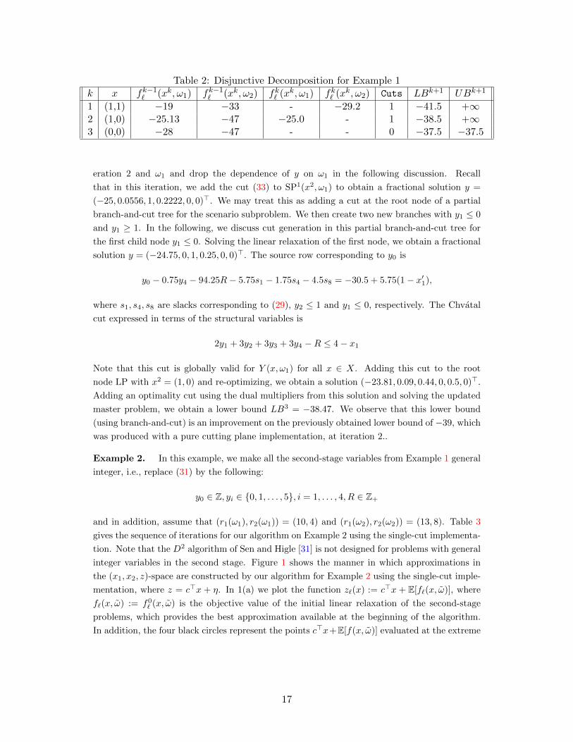
Table 2: Disjunctive Decomposition for Example 1

k x fk−1` (xk, ω1) fk−1

` (xk, ω2) fk` (xk, ω1) fk` (xk, ω2) Cuts LBk+1 UBk+1

1 (1,1) −19 −33 - −29.2 1 −41.5 +∞2 (1,0) −25.13 −47 −25.0 - 1 −38.5 +∞3 (0,0) −28 −47 - - 0 −37.5 −37.5

eration 2 and ω1 and drop the dependence of y on ω1 in the following discussion. Recall

that in this iteration, we add the cut (33) to SP1(x2, ω1) to obtain a fractional solution y =

(−25, 0.0556, 1, 0.2222, 0, 0)>. We may treat this as adding a cut at the root node of a partial

branch-and-cut tree for the scenario subproblem. We then create two new branches with y1 ≤ 0

and y1 ≥ 1. In the following, we discuss cut generation in this partial branch-and-cut tree for

the first child node y1 ≤ 0. Solving the linear relaxation of the first node, we obtain a fractional

solution y = (−24.75, 0, 1, 0.25, 0, 0)>. The source row corresponding to y0 is

y0 − 0.75y4 − 94.25R− 5.75s1 − 1.75s4 − 4.5s8 = −30.5 + 5.75(1− x′1),

where s1, s4, s8 are slacks corresponding to (29), y2 ≤ 1 and y1 ≤ 0, respectively. The Chvatal

cut expressed in terms of the structural variables is

2y1 + 3y2 + 3y3 + 3y4 −R ≤ 4− x1

Note that this cut is globally valid for Y (x, ω1) for all x ∈ X. Adding this cut to the root

node LP with x2 = (1, 0) and re-optimizing, we obtain a solution (−23.81, 0.09, 0.44, 0, 0.5, 0)>.

Adding an optimality cut using the dual multipliers from this solution and solving the updated

master problem, we obtain a lower bound LB3 = −38.47. We observe that this lower bound

(using branch-and-cut) is an improvement on the previously obtained lower bound of −39, which

was produced with a pure cutting plane implementation, at iteration 2..

Example 2. In this example, we make all the second-stage variables from Example 1 general

integer, i.e., replace (31) by the following:

y0 ∈ Z, yi ∈ 0, 1, . . . , 5, i = 1, . . . , 4, R ∈ Z+

and in addition, assume that (r1(ω1), r2(ω1)) = (10, 4) and (r1(ω2), r2(ω2)) = (13, 8). Table 3

gives the sequence of iterations for our algorithm on Example 2 using the single-cut implementa-

tion. Note that the D2 algorithm of Sen and Higle [31] is not designed for problems with general

integer variables in the second stage. Figure 1 shows the manner in which approximations in

the (x1, x2, z)-space are constructed by our algorithm for Example 2 using the single-cut imple-

mentation, where z = c>x + η. In 1(a) we plot the function z`(x) := c>x + E[f`(x, ω)], where

f`(x, ω) := f0` (x, ω) is the objective value of the initial linear relaxation of the second-stage

problems, which provides the best approximation available at the beginning of the algorithm.

In addition, the four black circles represent the points c>x+E[f(x, ω)] evaluated at the extreme

17

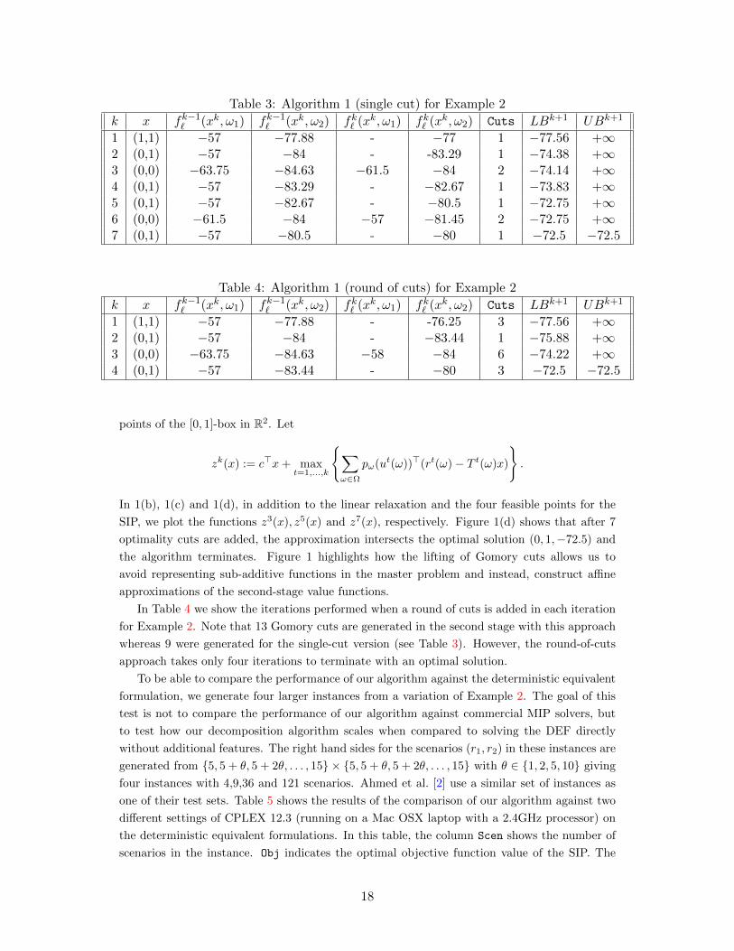
Table 3: Algorithm 1 (single cut) for Example 2

k x fk−1` (xk, ω1) fk−1

` (xk, ω2) fk` (xk, ω1) fk` (xk, ω2) Cuts LBk+1 UBk+1

1 (1,1) −57 −77.88 - −77 1 −77.56 +∞2 (0,1) −57 −84 - -83.29 1 −74.38 +∞3 (0,0) −63.75 −84.63 −61.5 −84 2 −74.14 +∞4 (0,1) −57 −83.29 - −82.67 1 −73.83 +∞5 (0,1) −57 −82.67 - −80.5 1 −72.75 +∞6 (0,0) −61.5 −84 −57 −81.45 2 −72.75 +∞7 (0,1) −57 −80.5 - −80 1 −72.5 −72.5

Table 4: Algorithm 1 (round of cuts) for Example 2

k x fk−1` (xk, ω1) fk−1

` (xk, ω2) fk` (xk, ω1) fk` (xk, ω2) Cuts LBk+1 UBk+1

1 (1,1) −57 −77.88 - -76.25 3 −77.56 +∞2 (0,1) −57 −84 - −83.44 1 −75.88 +∞3 (0,0) −63.75 −84.63 −58 −84 6 −74.22 +∞4 (0,1) −57 −83.44 - −80 3 −72.5 −72.5

points of the [0, 1]-box in R2. Let

zk(x) := c>x+ maxt=1,...,k

∑ω∈Ω

pω(ut(ω))>(rt(ω)− T t(ω)x)

.

In 1(b), 1(c) and 1(d), in addition to the linear relaxation and the four feasible points for the

SIP, we plot the functions z3(x), z5(x) and z7(x), respectively. Figure 1(d) shows that after 7

optimality cuts are added, the approximation intersects the optimal solution (0, 1,−72.5) and

the algorithm terminates. Figure 1 highlights how the lifting of Gomory cuts allows us to

avoid representing sub-additive functions in the master problem and instead, construct affine

approximations of the second-stage value functions.

In Table 4 we show the iterations performed when a round of cuts is added in each iteration

for Example 2. Note that 13 Gomory cuts are generated in the second stage with this approach

whereas 9 were generated for the single-cut version (see Table 3). However, the round-of-cuts

approach takes only four iterations to terminate with an optimal solution.

To be able to compare the performance of our algorithm against the deterministic equivalent

formulation, we generate four larger instances from a variation of Example 2. The goal of this

test is not to compare the performance of our algorithm against commercial MIP solvers, but

to test how our decomposition algorithm scales when compared to solving the DEF directly

without additional features. The right hand sides for the scenarios (r1, r2) in these instances are

generated from 5, 5 + θ, 5 + 2θ, . . . , 15 × 5, 5 + θ, 5 + 2θ, . . . , 15 with θ ∈ 1, 2, 5, 10 giving

four instances with 4,9,36 and 121 scenarios. Ahmed et al. [2] use a similar set of instances as

one of their test sets. Table 5 shows the results of the comparison of our algorithm against two

different settings of CPLEX 12.3 (running on a Mac OSX laptop with a 2.4GHz processor) on

the deterministic equivalent formulations. In this table, the column Scen shows the number of

scenarios in the instance. Obj indicates the optimal objective function value of the SIP. The

18

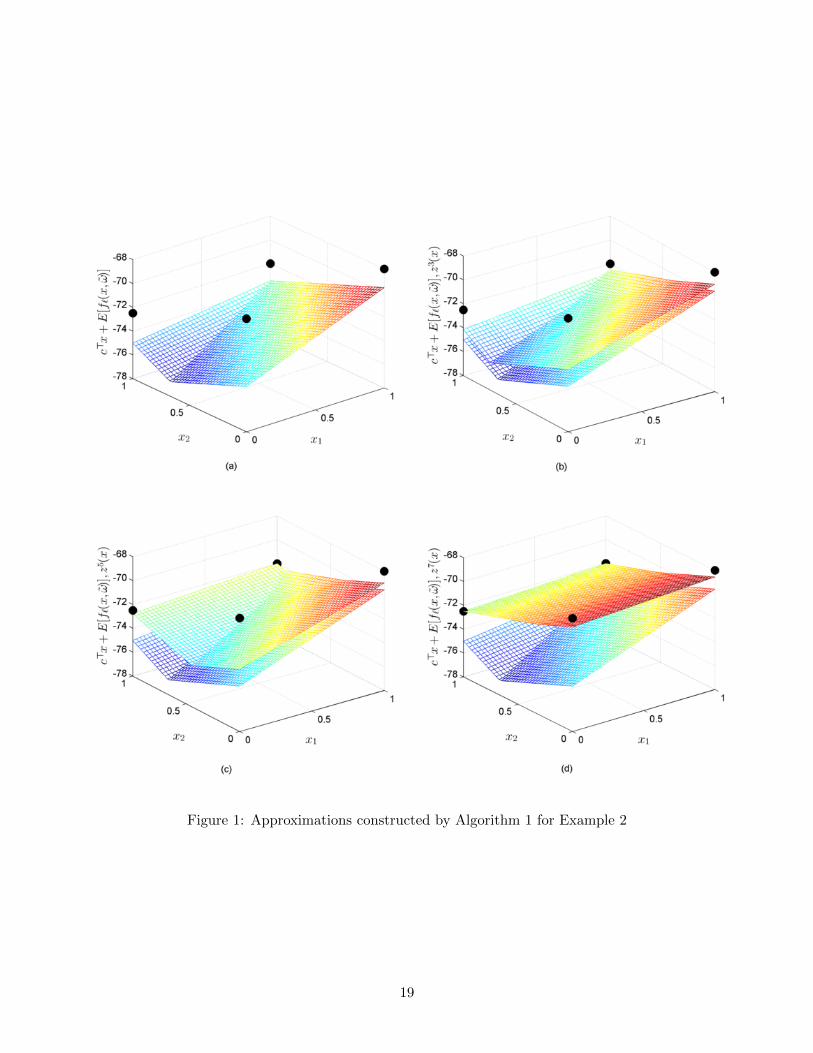
Figure 1: Approximations constructed by Algorithm 1 for Example 2

19

Table 5: Comparison of Algorithm 1 and the DEFScen Obj Vars Cons GDD-S GDD-R B&B B&B+Gom

4 −63.50 22 24 7 (0, 13) 7 (0, 32) 54 2 (6)9 −65.67 47 54 8(0, 43) 6 (0, 76) 324 19 (17)36 −66.83 182 216 10(1, 183) 6 (0, 384) 1.53E7∗ 206 (50)121 −67.17 607 726 10(1, 634) 6 (0, 1302) 7.52E6∗ 11359 (167)

columns Vars and Cons indicate the number of columns and rows in the deterministic equivalent

formulation, respectively. For entries under the columns GDD-S (single-cut) and GDD-R (round-

of-cuts), we report the number of iterations of the decomposition algorithm with Gomory cuts,

followed by two numbers within parentheses: the first number denotes the total number of non-

root nodes over all iterations explored by the CPLEX’s branch-and-bound tree for the master

program (stage 1) with cuts, presolve and heuristics turned off. The second number denotes the

total number of Gomory cuts added in the second stage over all iterations. Since our algorithmic

design includes only pure branch-and-bound (first-stage) and pure cutting planes in the second-

stage, our comparisons with CPLEX in this section is also done with comparable settings to

exclude any extraneous features. Thus, we compare two sets of runs using CPLEX: the column

B&B indicates the number of pure branch-and-bounds nodes explored by CPLEX on the DEF.

The column B&B + Gom shows the number of nodes explored by CPLEX along with the number

of cuts added in the parenthesis when we use pure branch-and-bound with Gomory cuts. The

solution times for all entries in the columns GDD-S, GDD-R, B&B, B&B + Cuts are less than 5

seconds, except when indicated by an asterisk. An asterisk next to an entry implies that the

stipulated time limit of 15 minutes was exceeded. It is important to note that these times are

obtained using a prototyping script (i.e. MATLAB), which is a far-cry from the technology

underlying CPLEX based on a C/C++ platform that has been developed over the past two

decades. In Section 7 we present an initial implementation of Algorithm 1 utilizing such a

platform.

From the columns GDD-S and GDD-R in Table 5, we see that the number of master problems

solved remains relatively stable as the number of scenarios increases. In addition, the master

programs are far smaller in size than the DEF, and as a result the total number of nodes explored

for the master problems is negligible for these instances. Although a larger number of cuts are

generated in the round-of-cuts version than the single-cut version, the additional computational

effort spent in deriving these cuts is trivial and moreover, the number of master programs solved

reduces significantly for the last three instances. When CPLEX branch-and-bound is run on

the DEF with cuts, presolve and heuristics turned off, the performance is quite poor for the

last two instances. In fact, CPLEX exceeds the time limit of 15 minutes after solving millions

of nodes for the last two instances. When Gomory cuts are turned on, CPLEX’s performance

improves with fewer nodes explored. However, even on these relatively small problems the lack

of scalability of the DEF is evident, as for the last instance, over eleven thousand branch-and-cut

nodes are explored by CPLEX. Based on the instances tested here we see that the number of

iterations of the decomposition-based cutting plane procedure is quite stable, relative to CPLEX

branch-and-bound or branch-and-cut on the DEF.

20

7 Preliminary Computational Experience

In this section, we describe a preliminary implementation of the decomposition algorithm with

Gomory cuts using the single-cut implementation. We implement the algorithm in C integrated

with IBM ILOG CPLEX 12.4 using the C callable library API where CPLEX is used to solve

the master problem and subproblems. We conduct our tests on a Windows XP operating system

running on a 2.66 GHz Intel CoreQuad processor with 4GB RAM. We compile our code using

Visual Studio 2008.

We test our implementation on instances of the stochastic server location problem (SSLP)

[26] with at least 50 scenarios. These instances are available online as a part of the stochastic

integer programming test problem library (SIPLIB). The original instances have B = 1, 2,C = 2 and D = ∅. We convert these instances to pure integer second stage by changing the

declaration of the continuous variables to integers. Our implementation also includes a version

of the lexicographic dual simplex described in [40, 1]. Although the lexicographic dual simplex is

needed for theoretical convergence, we do not observe a significant impact on our computational

tests on the SSLP test instances (see [15] for details). Hence, we report our tests with the regular

dual simplex method.

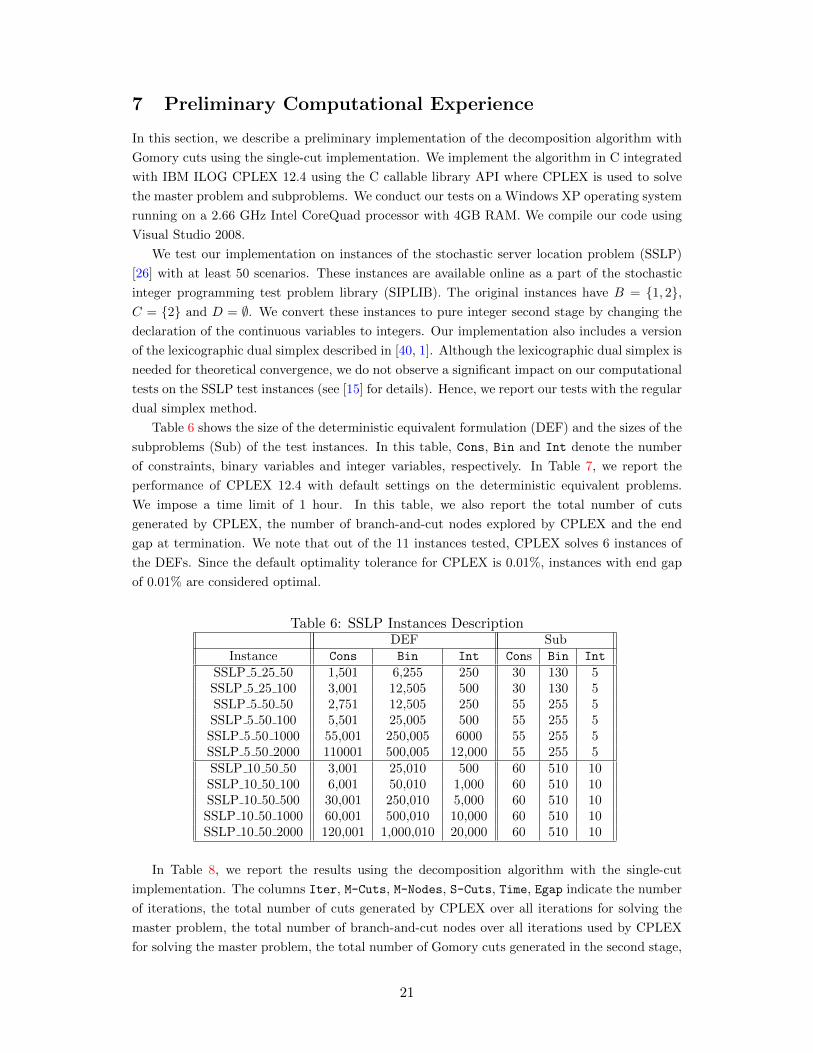
Table 6 shows the size of the deterministic equivalent formulation (DEF) and the sizes of the

subproblems (Sub) of the test instances. In this table, Cons, Bin and Int denote the number

of constraints, binary variables and integer variables, respectively. In Table 7, we report the

performance of CPLEX 12.4 with default settings on the deterministic equivalent problems.

We impose a time limit of 1 hour. In this table, we also report the total number of cuts

generated by CPLEX, the number of branch-and-cut nodes explored by CPLEX and the end

gap at termination. We note that out of the 11 instances tested, CPLEX solves 6 instances of

the DEFs. Since the default optimality tolerance for CPLEX is 0.01%, instances with end gap

of 0.01% are considered optimal.

Table 6: SSLP Instances DescriptionDEF Sub

Instance Cons Bin Int Cons Bin Int

SSLP 5 25 50 1,501 6,255 250 30 130 5SSLP 5 25 100 3,001 12,505 500 30 130 5SSLP 5 50 50 2,751 12,505 250 55 255 5SSLP 5 50 100 5,501 25,005 500 55 255 5SSLP 5 50 1000 55,001 250,005 6000 55 255 5SSLP 5 50 2000 110001 500,005 12,000 55 255 5SSLP 10 50 50 3,001 25,010 500 60 510 10SSLP 10 50 100 6,001 50,010 1,000 60 510 10SSLP 10 50 500 30,001 250,010 5,000 60 510 10SSLP 10 50 1000 60,001 500,010 10,000 60 510 10SSLP 10 50 2000 120,001 1,000,010 20,000 60 510 10

In Table 8, we report the results using the decomposition algorithm with the single-cut

implementation. The columns Iter, M-Cuts, M-Nodes, S-Cuts, Time, Egap indicate the number

of iterations, the total number of cuts generated by CPLEX over all iterations for solving the

master problem, the total number of branch-and-cut nodes over all iterations used by CPLEX

for solving the master problem, the total number of Gomory cuts generated in the second stage,

21

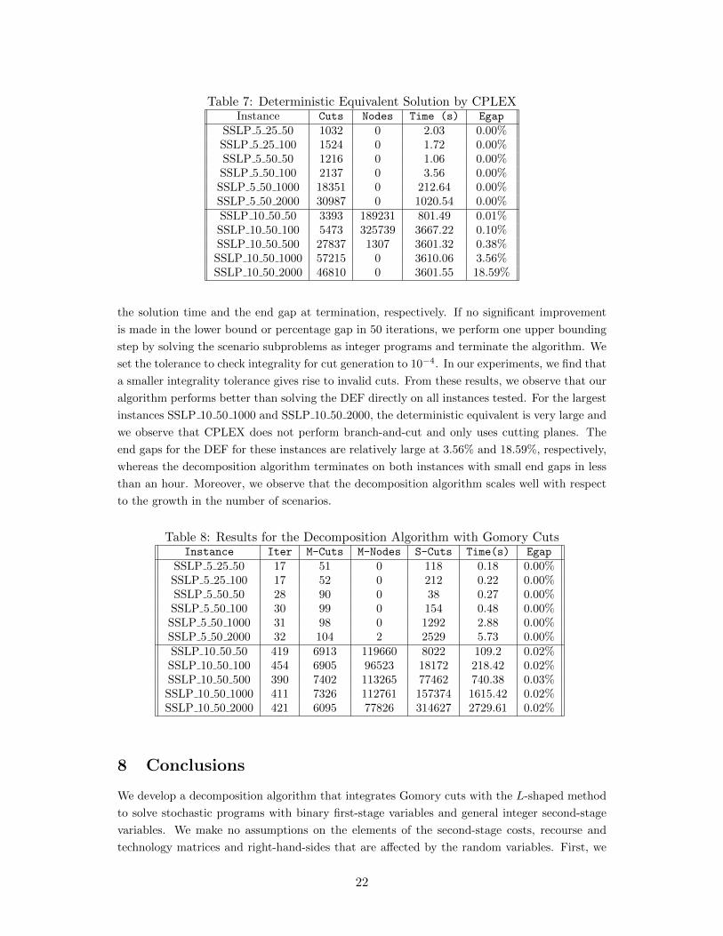
Table 7: Deterministic Equivalent Solution by CPLEXInstance Cuts Nodes Time (s) Egap

SSLP 5 25 50 1032 0 2.03 0.00%SSLP 5 25 100 1524 0 1.72 0.00%SSLP 5 50 50 1216 0 1.06 0.00%SSLP 5 50 100 2137 0 3.56 0.00%SSLP 5 50 1000 18351 0 212.64 0.00%SSLP 5 50 2000 30987 0 1020.54 0.00%SSLP 10 50 50 3393 189231 801.49 0.01%SSLP 10 50 100 5473 325739 3667.22 0.10%SSLP 10 50 500 27837 1307 3601.32 0.38%SSLP 10 50 1000 57215 0 3610.06 3.56%SSLP 10 50 2000 46810 0 3601.55 18.59%

the solution time and the end gap at termination, respectively. If no significant improvement

is made in the lower bound or percentage gap in 50 iterations, we perform one upper bounding

step by solving the scenario subproblems as integer programs and terminate the algorithm. We

set the tolerance to check integrality for cut generation to 10−4. In our experiments, we find that

a smaller integrality tolerance gives rise to invalid cuts. From these results, we observe that our

algorithm performs better than solving the DEF directly on all instances tested. For the largest

instances SSLP 10 50 1000 and SSLP 10 50 2000, the deterministic equivalent is very large and

we observe that CPLEX does not perform branch-and-cut and only uses cutting planes. The

end gaps for the DEF for these instances are relatively large at 3.56% and 18.59%, respectively,

whereas the decomposition algorithm terminates on both instances with small end gaps in less

than an hour. Moreover, we observe that the decomposition algorithm scales well with respect

to the growth in the number of scenarios.

Table 8: Results for the Decomposition Algorithm with Gomory CutsInstance Iter M-Cuts M-Nodes S-Cuts Time(s) Egap

SSLP 5 25 50 17 51 0 118 0.18 0.00%SSLP 5 25 100 17 52 0 212 0.22 0.00%SSLP 5 50 50 28 90 0 38 0.27 0.00%SSLP 5 50 100 30 99 0 154 0.48 0.00%SSLP 5 50 1000 31 98 0 1292 2.88 0.00%SSLP 5 50 2000 32 104 2 2529 5.73 0.00%SSLP 10 50 50 419 6913 119660 8022 109.2 0.02%SSLP 10 50 100 454 6905 96523 18172 218.42 0.02%SSLP 10 50 500 390 7402 113265 77462 740.38 0.03%SSLP 10 50 1000 411 7326 112761 157374 1615.42 0.02%SSLP 10 50 2000 421 6095 77826 314627 2729.61 0.02%

8 Conclusions

We develop a decomposition algorithm that integrates Gomory cuts with the L-shaped method

to solve stochastic programs with binary first-stage variables and general integer second-stage

variables. We make no assumptions on the elements of the second-stage costs, recourse and

technology matrices and right-hand-sides that are affected by the random variables. First, we

22

address the question whether the expected recourse function E[f(x, ω)] can be approximated by

a lower bounding problem that has the same properties as a Benders’ master problem. We show

that the algorithm generates piecewise linear convex approximations of the expected recourse

function. Next, we address the question on devising an algorithm that avoids solving the scenario

subproblems to integer optimality in every iteration. Our algorithm iteratively constructs LP-

based approximations of the integer second-stage subproblems. Finally, we address the issue of

finite convergence of a decomposition algorithm that uses only cutting planes to approximate the

second-stage subproblems by developing parameterized Gomory cuts that are constructed using

relatively simple operations. Although Gomory cuts for SIP were first introduced in a conceptual

framework in Carøe and Tind [12], we believe that our algorithm is the first incorporation of

parametric Gomory cuts within the L-shaped method that creates computationally amenable

first-stage approximations for two-stage SIP. Further, we show that the nature of convergence

of our algorithm has a robust characterization in that it can be extended to numerous settings

and allowing alternative implementations without the need to modify the convergence proofs.

As a result of our development, we can now allow both parametric disjunctive as well as

parametric Gomory cuts to be included within finitely convergent decomposition algorithms

for SIP. Such disparate collections of cuts have proven to be indispensable for the success of

branch-and-cut algorithms in deterministic MIP, and we are hopeful that the introduction of

Gomory cuts within a decomposition algorithm will be just as valuable for SIP. Our prelimi-

nary computational results are promising and demonstrate the scalability of our algorithm with

respect to the growth in the number of scenarios. A detailed computational study of the algo-

rithms developed here with the lexicographic dual simplex method and other extensions will be

reported in a subsequent paper.

Acknowledgment

We thank the two referees for their suggestions that improved the paper.

References

1. Achterberg, T.: SCIP: solving constraint integer programs. Mathematical Programming

Computation 1(1), 1–41 (2009)

2. Ahmed, S., Tawarmalani, M., Sahinidis, N.: A finite branch-and-bound algorithm for two-

stage stochastic integer programs. Mathematical Programming 100(2), 355–377 (2004)

3. Balas, E., Ceria, S., Cornuejols, G.: A lift-and-project cutting plane algorithm for mixed

0–1 programs. Mathematical Programming 58(1), 295–324 (1993)

4. Balas, E., Ceria, S., Cornuejols, G., Natraj, N.: Gomory cuts revisited. Operations Research

Letters 19(1), 1–9 (1996)

5. Benders, J.: Partitioning procedures for solving mixed-variables programming problems.

Numerische Mathematik 4(1), 238–252 (1962)

6. Birge, J., Louveaux, F.: A multicut algorithm for two-stage stochastic linear programs.

European Journal of Operational Research 34(3), 384–392 (1988)

23

7. Birge, J., Louveaux, F.: Introduction to stochastic programming. 2 edn. Springer (2011)

8. Bixby, R., Rothberg, E.: Progress in computational mixed integer programming: a look

back from the other side of the tipping point. Annals of Operations Research 149(1), 37–41

(2007)

9. Blair, C., Jeroslow, R.: The value function of an integer program. Mathematical Program-

ming 23(1), 237–273 (1982)

10. Borozan, V., Cornuejols, G.: Minimal valid inequalities for integer constraints. Mathematics

of Operations Research 34(3), 538–546 (2009)

11. Carøe, C., Tind, J.: A cutting-plane approach to mixed 0-1 stochastic integer programs.

European Journal of Operational Research 101(2), 306–316 (1997)

12. Carøe, C., Tind, J.: L-shaped decomposition of two-stage stochastic programs with integer

recourse. Mathematical Programming 83(1), 451–464 (1998)

13. Chen, B., Kucukyavuz, S., Sen, S.: Finite disjunctive programming characterizations for

general mixed-integer linear programs. Operations Research 59(1), 202–210 (2011)

14. Chvatal, V.: Edmonds polytopes and a hierarchy of combinatorial problems. Discrete

Mathematics 4(4), 305–337 (1973)

15. Gade, D.: Algorithms and reformulations for large-scale integer and stochastic integer pro-

grams. Ph.D. thesis, The Ohio State University (2012)

16. Gomory, R.: Outline of an algorithm for integer solutions to linear programs. Bulletin of

the American Mathematical Society 64(5), 275–278 (1958)

17. Gomory, R.: An algorithm for the mixed integer problem. Tech. Rep. RM-2597, RAND

Corporation (1960)

18. Gomory, R.: Some polyhedra related to combinatorial problems. Linear Algebra and its

Applications 2(4), 451–558 (1969)

19. Kong, N., Schaefer, A., Hunsaker, B.: Two-stage integer programs with stochastic right-

hand sides: a superadditive dual approach. Mathematical Programming 108(2), 275–296

(2006)

20. Laporte, G., Louveaux, F.: The integer L-shaped method for stochastic integer programs

with complete recourse. Operations Research Letters 13(3), 133–142 (1993)

21. Louveaux, F., Schultz, R.: Stochastic integer programming. In: Shapiro, A., Ruszczynski,

A. (eds.) Stochastic Programming, Handbooks in Operations Research and Management

Science, vol. 10, pp. 213–266. Elsevier (2003)

22. Mayr, E.: Some complexity results for polynomial ideals. Journal of complexity 13(3),

303–325 (1997)

24

23. Nemhauser, G., Wolsey, L.: Integer and combinatorial optimization. John Wiley & Sons,

New York (1988)

24. Nourie, F., Venta, E.: An upper bound on the number of cuts needed in Gomory’s method

of integer forms. Operations Research Letters 1(4), 129–133 (1982)

25. Ntaimo, L.: Disjunctive decomposition for two-stage stochastic mixed-binary programs with

random recourse. Operations Research 58(1), 229–243 (2010)

26. Ntaimo, L., Sen, S.: The million-variable march for stochastic combinatorial optimization.

Journal of Global Optimization 32(3), 385–400 (2005)

27. Ntaimo, L., Sen, S.: A comparative study of decomposition algorithms for stochastic combi-

natorial optimization. Computational Optimization and Applications 40(3), 299–319 (2008)

28. Schultz, R.: Continuity properties of expectation functions in stochastic integer program-

ming. Mathematics of Operations Research 18(3), 578–589 (1993)

29. Schultz, R., Stougie, L., van der Vlerk, M.: Solving stochastic programs with integer re-

course by enumeration: A framework using Grobner basis. Mathematical Programming

83(1), 229–252 (1998)

30. Sen, S.: Algorithms for stochastic mixed-integer programming models. In: Aardal, K.,

Nemhauser, G., Weismantel, R. (eds.) Discrete Optimization, Handbooks in Operations

Research and Management Science, vol. 12, pp. 515–558. Elsevier (2003)

31. Sen, S., Higle, J.: The C3 theorem and a D2 algorithm for large scale stochastic mixed-

integer programming: set convexification. Mathematical Programming 104(1), 1–20 (2005)

32. Sen, S., Higle, J., Ntaimo, L.: A summary and illustration of disjunctive decomposition

with set convexification. In: Woodruff, D. (ed.) Network Interdiction and Stochastic Integer

Programming, pp. 105–125. Springer (2003)

33. Sen, S., Sherali, H.: On the convergence of cutting plane algorithms for a class of nonconvex

mathematical programs. Mathematical Programming 31(1), 42–56 (1985)

34. Sen, S., Sherali, H.: Decomposition with branch-and-cut approaches for two-stage stochastic

mixed-integer programming. Mathematical Programming 106(2), 203–223 (2006)

35. Sherali, H., Adams, W.: A reformulation-linearization technique for solving discrete and

continuous nonconvex problems, Nonconvex Optimization and its Applications, vol. 31.

Kluwer Academic Publishers (1999)

36. Sherali, H., Fraticelli, B.: A modification of Benders’ decomposition algorithm for discrete

subproblems: An approach for stochastic programs with integer recourse. Journal of Global

Optimization 22(1), 319–342 (2002)

37. Sherali, H., Zhu, X.: On solving discrete two-stage stochastic programs having mixed-integer

first-and second-stage variables. Mathematical Programming 108(2), 597–616 (2006)

25

38. Van Slyke, R., Wets, R.: L-shaped linear programs with applications to optimal control and

stochastic programming. SIAM Journal of Applied Mathematics 17(4), 638–663 (1969)

39. Yuan, Y., Sen, S.: Enhanced cut generation methods for decomposition-based branch and

cut for two-stage stochastic mixed-integer programs. INFORMS Journal on Computing

21(3), 480–487 (2009)

40. Zanette, A., Fischetti, M., Balas, E.: Lexicography and degeneracy: can a pure cutting

plane algorithm work? Mathematical Programming 130(1), 1–24 (2010)

26