Decomposing Wage Distributions using Recentered

Influence Function Regressions

Sergio Firpo

PUC-Rio

Nicole Fortin

UBC

Thomas Lemieux

UBC and NBER

June 2007

Abstract

We propose a two-stage procedure to decompose changes or differences in the

distribution of wages (or of other variables). In the first stage, distributional

changes are divided into a wage structure effect and a composition effect using

a reweighting method. The reweighting allows us to estimate directly these two

components of the decomposition without having to estimate a structural wage-

setting model. In the second stage, the two components are further divided into the

contribution of each explanatory variable using novel recentered influence function

(RIF) regressions. These regressions estimate directly the impact of the explana-

tory variables on the distributional statistic of interest. The paper generalizes the

popular Oaxaca-Blinder decomposition method by extending the decomposition to

any distributional measure (besides the mean) and by allowing for a much more

flexible wage setting model. We illustrate the practical aspects of the procedure

by analyzing how polarization of U.S. male wages that took place between the late

1980s and the mid 2000s was affected by factors such as de-unionization, education,

occupations and industry changes.

1 Introduction

Distributional issues have attracted a lot of attention in labor economics over the last

fifteen years. One important factor behind the resurgence of interest for distributional

issues is the large increase in wage inequality in the United States and several other coun-

tries. There is also growing literature looking at wages differentials between subgroups

that goes beyond simple mean comparisons. For example, several recent papers such

as Albrecht, Bjorklund and Vroman (2003) look at whether the gender gap is larger in

the upper tail than in the lower tail of the wage distribution because of a “glass ceil-

ing”. More generally, there is increasing interest for distributional impacts of various

programs or interventions. In all these cases, the key question of economic interest is

which factors account for changes (or differences) in distributions. For example, did

wage inequality increase because education or other wage setting factors became more

unequally distributed, or because the return to these factors changed over time?

In response to these important questions, a number of decomposition procedures have

been suggested to untangle the sources of changes or differences in wage distributions.

Popular methods used in the wage inequality literature include the “plug-in” proce-

dure of Juhn, Murphy, and Pierce (1993), the reweighting procedure of DiNardo, Fortin,

and Lemieux (1996), and, more recently, the quantile-based decomposition method of

Machado and Mata (2005).1 Unfortunately, none of these methods can be used to de-

compose general distributional measures in the same way means can be decomposed using

the conventional Oaxaca-Blinder method.

As is well known, the Oaxaca-Blinder procedure provides a way of 1) decomposing

changes or differences in mean wages into a wage structure effect and a composition effect,

and 2) further dividing these two components into the contribution of each covariate. The

leading problem with the above mentioned decomposition methods is that they cannot

be used to divide the composition effect into the role of each covariate. So while it is

natural to ask to what extent changes in the distribution of education have contributed

to the growth in wage inequality, this particular question has not been answered in the

literature for lack of available decomposition methods. Similarly, we do not know the

contribution of male-female differences in experience to the male-female difference in

median wages for lack of available methods. In contrast, this question is straightforward

to answer in the case of the mean using a Oaxaca-Blinder decomposition.

In this paper, we propose a two-stage procedure to perform Oaxaca-Blinder type

1See also Gosling, Machin and Meghir (2000) for a related quantile decomposition method.

1

decompositions on any distributional measure, and not only the mean. The first stage

of our approach consists of decomposing the distributional statistic of interest into a

wage structure and a composition component using a reweighting approach, where the

weights are either parametrically or non-parametrically estimated. As in the related

program evaluation literature, we show that ignorability and common support are key

assumptions required to identify separately the wage structure and composition effects.

Provided that these assumptions are satisfied, the underlying wage setting model can be

as general as possible. The idea of the first stage is thus very similar to DiNardo, Fortin,

and Lemieux (1996). A first contribution here is to clarify the assumptions required for

identification, in the case of other distributional statistics besides the mean, by drawing a

parallel with the program evaluation (treatment effect) literature. A related contribution

is to provide analytical formulas for the standard errors of the reweighting estimates.

In the second stage, we further divide the wage structure and composition effects

into the contribution of each covariate, just as in the usual Oaxaca-Blinder decompo-

sition. This is done using a novel regression-based method proposed by Firpo, Fortin,

and Lemieux (2006) to estimate the effect of changes in covariates on any distributional

statistics such as the median, inter-quartile ranges, or the Gini coefficient. The idea of

the method is to replace the dependent variable by the corresponding recentered influ-

ence function (RIF) for the distributional statistics of interest. The influence function is

a widely used concept in robust statistics and is easy to compute. As a result, the (re-

centered) influence function regressions proposed by Firpo, Fortin, and Lemieux (2006)

are as easy to estimate as ordinary least squares regressions.

We illustrate how our procedure works in practice by looking at changes in the dis-

tribution of male wages in the United States between the late 1980s and the mid 2000s.

This period is quite interesting from a distributional point of view as inequality increased

in the top end of the wage distribution, but decreased in the low end of the distribution,

a phenomena that Autor, Katz and Kearney (2006) have called the polarization of the

U.S. labor market. We use our method to investigate the source of change in wages at

different points of the wage distribution by decomposing the changes at various wage

quantiles. The results indicate that no single factor appears to be able to explain the

polarization of the labor market. De-unionization accounts for some of the decreasing

wage inequality at the low end and increasing inequality at the top end. The continu-

ing growth in returns to education, especially at a level above high school, is the most

important source of growth in top-end inequality, but it cannot explain changes at the

low-end. Changes in industrial and occupational structure of the workforce, and in the

2

effect of industry and occupation, explain very little of the changes in inequality. This

suggest that explanations such as the growth in high-tech sectors or the wage decline in

“routine occupations” (Autor, Levy, and Murnane, 2003) have little impact on changes

in the wage distribution, once education and other factors are controlled for.2

The remainder of the paper is organized as follows. Section 2 discusses the decom-

position problem and reviews the strengths and weaknesses of existing procedures. The

identification of the proposed decomposition procedure is addressed in Section 3. Section

4 discusses estimation and inference, and illustrates how the decomposition methodology

works in the case of the mean, the median, and the variance. Section 5 provides an em-

pirical application of the methodology to the changes in the distribution of male wages

in the United States between the late 1980s and the mid 2000s.

2 The Decomposition Problem and Shortcomings of

Existing Methods

Before presenting our method in detail, it is useful to first review the case of the mean

for which the standard Oaxaca-Blinder method is very well known. To simplify the

exposition of the paper, we will work with the case where the outcome variable, Y , is the

wage, though our approach can be used for any other outcome variable. The Oaxaca-

Blinder method can be used to divide a difference in mean wages between two groups,

or overall mean wage gap, into a composition effect linked to differences in covariates

between the two groups, and a wage structure effect linked to differences in the return to

these covariates between the two groups. The two groups are labelled as t = 0, 1. In the

original papers by Oaxaca (1974) and Blinder (1973), the two groups used were either

men and women, or blacks and whites. More generally, the two groups can be a control

and a treatment group, or similar groups of individuals at two points in time, as in the

wage inequality literature.

We first review how the Oaxaca-Blinder decomposition provides a straightforward

way of dividing up the contribution of each covariate to both composition and wage

structure effects. We then move to the case of more general distributional parameters to

point out that existing methods do not provide a way of decomposing differences in these

distributional parameters into the contribution of each covariate (to the composition and

wage structure effect).

2Indeed, the growth in returns to insurance, real estate and financial sales occupations dwarfs thegrowth in returns to high tech occupations, such as engineering and computer occupations.

3

2.1 The Mean

We focus on differences in the wage distributions of two groups, 1 and 0. For a worker

i, let Y1i be the wage that would be paid in group 1, and Y0i the wage that would be

paid in group 0. Since a given individual i is only observed in one of the two groups, we

either observe Y1i or Y0i, but never both. Therefore, for each i we can define the observed

wage, Yi, as Yi = Y1i · Ti + Y0i · (1 − Ti), where Ti = 1 if individual i is observed in group

1, and Ti = 0 if individual i is observed in group 0. There is also a vector of covariates

X ∈ X ⊂ RK that we can observe in both groups.

In the standard Oaxaca-Blinder decomposition, the conditional expectation of Y given

X is assumed to be linear so that

E[Yti|X] = Xiβt + εti, for t = 0, 1. (1)

where E[εti|Xi, T = t] = 0. Define the overall mean wage gap as ∆µO, and consider

dividing the overall mean gap into a wage structure effect, ∆µS and a composition effect,

∆µX . Averaging over X, the mean wage gap ∆µ

O can be written as

∆µO = E[E(Y |X,T = 1)] − E[E(Y |X,T = 0)]

= E[Y |T = 1] − E[Y |T = 0]

= E [X|T = 1]β1 + E [ε1|T = 1] − (E [X|T = 0] β0 + E [ε0|T = 0])

Under the linearity assumption, E [εt|T = t] = 0 because E [εt|X,T = t] = 0, and the

expression reduces to

∆µO = E [X|T = 1]β1 − E [X|T = 0] β0

= E [X|T = 1] (β1 − β0) + (E [X|T = 1] − E [X|T = 0]) β0

= ∆µS + ∆µ

X,

The first term on the next to last line of the equation is the wage structure effect,

∆µS , while the second term is the composition effect, ∆µ

X. Note that the reference group

used to compute the wage structure here is the group 1, though the decomposition could

also be performed using group 0 instead as the reference group. The wage structure and

4

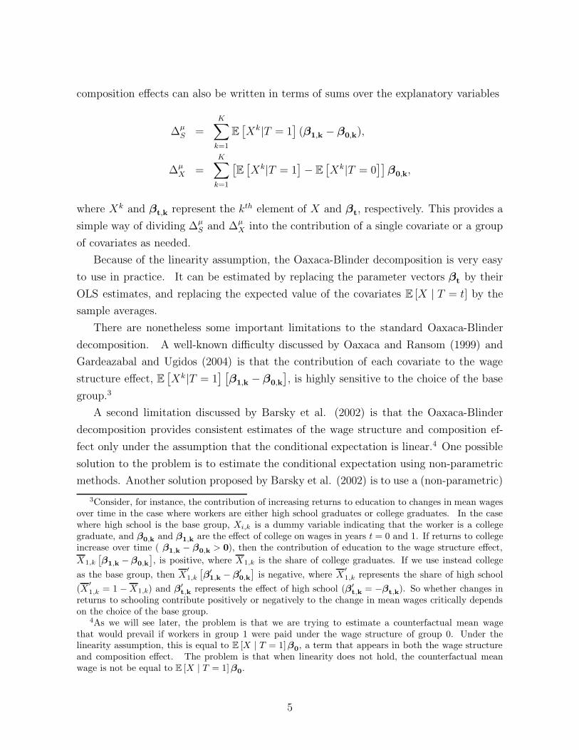
composition effects can also be written in terms of sums over the explanatory variables

∆µS =

K∑

k=1

E[Xk|T = 1

](β1,k − β0,k),

∆µX =

K∑

k=1

[E[Xk|T = 1

]− E

[Xk|T = 0

]]β0,k,

where Xk and βt,k represent the kth element of X and βt, respectively. This provides a

simple way of dividing ∆µS and ∆µ

X into the contribution of a single covariate or a group

of covariates as needed.

Because of the linearity assumption, the Oaxaca-Blinder decomposition is very easy

to use in practice. It can be estimated by replacing the parameter vectors βt by their

OLS estimates, and replacing the expected value of the covariates E [X | T = t] by the

sample averages.

There are nonetheless some important limitations to the standard Oaxaca-Blinder

decomposition. A well-known difficulty discussed by Oaxaca and Ransom (1999) and

Gardeazabal and Ugidos (2004) is that the contribution of each covariate to the wage

structure effect, E[Xk|T = 1

] [β1,k − β0,k

], is highly sensitive to the choice of the base

group.3

A second limitation discussed by Barsky et al. (2002) is that the Oaxaca-Blinder

decomposition provides consistent estimates of the wage structure and composition ef-

fect only under the assumption that the conditional expectation is linear.4 One possible

solution to the problem is to estimate the conditional expectation using non-parametric

methods. Another solution proposed by Barsky et al. (2002) is to use a (non-parametric)

3Consider, for instance, the contribution of increasing returns to education to changes in mean wagesover time in the case where workers are either high school graduates or college graduates. In the casewhere high school is the base group, Xi,k is a dummy variable indicating that the worker is a collegegraduate, and β0,k and β1,k are the effect of college on wages in years t = 0 and 1. If returns to collegeincrease over time ( β1,k − β0,k > 0), then the contribution of education to the wage structure effect,X1,k

[β1,k − β0,k

], is positive, where X1,k is the share of college graduates. If we use instead college

as the base group, then X′1,k

[β′

1,k − β′0,k

]is negative, where X

′1,k represents the share of high school

(X′1,k = 1 − X1,k) and β′

t,k represents the effect of high school (β′t,k = −βt,k). So whether changes in

returns to schooling contribute positively or negatively to the change in mean wages critically dependson the choice of the base group.

4As we will see later, the problem is that we are trying to estimate a counterfactual mean wagethat would prevail if workers in group 1 were paid under the wage structure of group 0. Under thelinearity assumption, this is equal to E [X | T = 1]β0, a term that appears in both the wage structureand composition effect. The problem is that when linearity does not hold, the counterfactual meanwage is not be equal to E [X | T = 1]β0.

5

reweighting approach as in DiNardo, Fortin and Lemieux (1996) to perform the decom-

position. The advantage of this solution is that it can be applied to more general

distributional statistics. The disadvantage of both of these solutions, however, is that

they do not provide direct ways, in general, of further dividing the contribution of each

covariate to the wage structure and composition effects.5

2.2 Other Distributional Statistics

The reweighting procedure proposed by DiNardo, Fortin and Lemieux (1996) provides

consistent estimates of the wage structure and composition effects for any distributional

statistic of interest under a set of assumptions discussed later in the paper. What this

type of procedure does not provide, however, is a general way further dividing up the

contribution of each single covariate to the wage structure and composition effect. One

exception is the case of dummy covariates where a conditional reweighting procedure can

then be used.6 One problem is that this approach is not easily extended to covariates

other than dummy variables. Furthermore, with many dummy covariates, one would

have to compute a large number of conditional reweighting factors to account for the

contribution of each covariate.

In the case of quantiles, Machado and Mata (2005) propose a decomposition proce-

dure based on (conditional) quantile regression methods.7 They consider the following

regression model for the τ th quantile of Y conditional on the covariates X (τ goes from

0 to 1):

Qτ(Y |X) = Xβ(τ ).

In principle, running such quantile regressions for all possible quantiles should describe

5We discuss the case of reweighting in more detail below. In the case where the conditional expectationE(Yi|Xi, T = t) is estimated non-parametrically, a whole different procedure would have to be used toseparate the wage structure into the contribution of each covariate. For instance, average derivativemethods could be used to estimate an effect akin to the β coefficients used in standard decompositions.Unfortunately, these methods are difficult to use in practice, and would not be helpful in dividing upthe composition effect into the contribution of each individual covariate.

6Both DiNardo and Lemieux (1997) and DiNardo, Fortin, and Lemieux (1996) discuss the case wherethe dummy covariate is union status. DiNardo and Lemieux (1997) compute a “total” effect of unionsby contrasting the actual distribution of wages to the distribution among non-union workers reweightedto have the same characteristics as the whole sample of workers. DiNardo, Fortin, and Lemieux (1996)compute the contribution of unions to the composition effect by contrasting actual changes in the wagedistribution to changes that would have prevailed if the rate of unionization, conditional on other charac-teristics, had remained constant over time. The contribution of unions to the wage structure effect canthen be obtained by taking the difference between the total contribution of unions and the contributionof unions to the composition effect only.

7See also Albrecht, van Vuuren and Vroman (2004) for more details on the Machado Mata procedure.

6

the whole conditional distribution of wages. One can then use the β(τ ) estimated for

one group to construct a counterfactual distribution for the other group, and then use

this counterfactual distribution to compute the overall composition and wage structure

effect.8 Furthermore, if one plugs in the β(τ ) pertaining to a single covariate only, it is

then possible to estimate the contribution of this covariate to the wage structure effect,

as in the Oaxaca-Blinder decomposition.

There are however, a number of drawbacks to this procedure. First and foremost,

it does not provide a way of dividing up the composition effect into the contribution of

each single covariate.9 Second, it is computationally difficult to implement as it involves

estimating a large number of quantile regressions, and conducting large scale simulations.

Third, as in the case of the mean, the decomposition is only consistent if the right

functional form is used for quantiles. Since the right functional form has to be chosen

for each and every quantiles, making sure that the specification is correct is a very difficult

empirical exercise.10

Other methods have been suggested by Juhn, Murphy, and Pierce (1993), Fortin

and Lemieux (1998) and Donald, Green, and Paarsch (2000) to decompose changes in

distributional statistics beyond the mean. These procedures have various strengths and

weaknesses. Most importantly, they all share the same shortcoming as Machado and

Mata (2005) in that they do not provide a way of dividing up the composition effect into

the contribution of each individual covariate.

In summary, currently available methods can be used to compute the overall wage

structure and composition effects for various distributional statistics. We build on this in

8Both Machado and Mata (2005) and Albrecht et al. (2003) use conditional quantile regressions toconstruct counterfactual unconditional wage distribution. Machado and Mata (2005) draw n numbersat random to choose the quantiles, estimate the conditional quantile coefficients from the first group,then for each quantile draw a random sample from the covariates of the alternate group and generatethe counterfactual wages. Albrecht et al. (2003) modify this procedure by choosing quantiles 1 through99, and by taking 100 draws for each quantile.

9Machado and Mata (2005) suggest using an unconditional reweighting procedure to compute thecontribution of a covariate to the composition effect. For example, in the case of unions, they wouldsuggest reweighting all union (or non-union) observations by a fixed factor. Unfortunately, doing soalso changes the distribution of other covariates that are differently distributed in the union and non-union sectors. As a result, the proposed procedure does not provide an estimate of the contribution ofunions, holding the distribution of other covariates fixed. Doing so would require using a conditionalreweighting factor, as in DiNardo, Fortin and Lemieux (1996). As discussed above, it is not clear howthis can be implemented when covariates are not dummy variables. Furthermore, if one uses these typesof reweighting procedures anyway, then everything that can be computed using the Machado and Mataprocedure can also be computed using a (simpler) reweighting procedure.

10Furthermore, if the correct functional form is not linear, it is then difficult to compute the contri-bution of each covariate to the wage structure effect, since there is no longer a single β(θ) coefficientassociated to a given covariate, as in the linear case.

7

the current paper by suggesting to estimate these two overall effects using a reweighting

procedure. Available methods are much more limited, however, when it comes to further

dividing the wage structure and, especially, the composition effect into the contribution

each covariate. The main contribution of the paper is to suggest a simple regression-

based procedure to remedy this shortcoming building on recent work by Firpo, Fortin,

and Lemieux (2006).

3 Identification

3.1 Wage Structure and Composition Effects

Following the treatment effect literature (Rosenbaum and Rubin, 1983, Heckman 1990,

Heckman and Robb 1985, 1986), we focus on differences in the wage distributions between

two groups, 1 and 0, or the “group effect”. Suppose we could observe a random sample

of N = N1 + N0 individuals, where N1 and N0 are the number of individuals in each

group and we index individuals by i = 1, . . . , N . We define the probability that an

individual i is in group 1 as p, whereas the conditional probability that an individual i

is in group 1 given X = x, is p(x) = Pr[T = 1|X = x], sometimes simply called the

“propensity-score”.

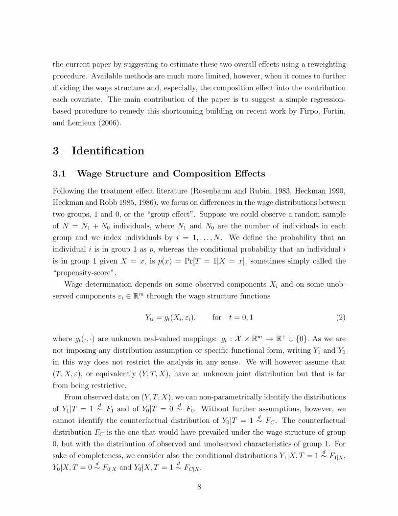
Wage determination depends on some observed components Xi and on some unob-

served components εi ∈ Rm through the wage structure functions

Yti = gt(Xi, εi), for t = 0, 1 (2)

where gt(·, ·) are unknown real-valued mappings: gt : X × Rm → R+ ∪ {0}. As we are

not imposing any distribution assumption or specific functional form, writing Y1 and Y0

in this way does not restrict the analysis in any sense. We will however assume that

(T,X, ε), or equivalently (Y, T,X), have an unknown joint distribution but that is far

from being restrictive.

From observed data on (Y, T,X), we can non-parametrically identify the distributions

of Y1|T = 1d∼ F1 and of Y0|T = 0

d∼ F0. Without further assumptions, however, we

cannot identify the counterfactual distribution of Y0|T = 1d∼ FC . The counterfactual

distribution FC is the one that would have prevailed under the wage structure of group

0, but with the distribution of observed and unobserved characteristics of group 1. For

sake of completeness, we consider also the conditional distributions Y1|X,T = 1d∼ F1|X,

Y0|X,T = 0d∼ F0|X and Y0|X,T = 1

d∼ FC|X.

8

We typically analyze the difference in wage distributions between groups 1 and 0 by

looking at some functionals of these distributions. Let ν be a functional of the conditional

joint distribution of (Y1, Y0) |T , that is ν : Fν → R, and Fν is a class of distribution

functions such that F ∈ Fν if ‖ν (F )‖ < +∞. The difference in the ν’s between the two

groups is called here the ν-overall wage gap, which is basically the difference in wages

measured in terms of the distributional statistic ν:11

∆νO = ν (F1) − ν (F0) = ν1 − ν0. (3)

We can use the fact that X is potentially unevenly distributed across groups to

decompose equation (3) into two parts:

∆νO = (ν1 − νC) + (νC − ν0) = ∆ν

S + ∆νX (4)

where the first term ∆νS reflects the effect of differences in the “wage structure”, which is

summarized by the gt(·, ·) functions. Therefore, this first term corresponds to the effect

on ν of a change from g1(·, ·) to g0(·, ·) keeping the distribution of (X, ε)|T = 1 constant.

With no other restrictions, the second term ∆νX will correspond to effects of changes in

the distribution of (X, ε), keeping the “wage structure” g0(·, ·) constant, that is, the effect

of changes in distribution from the one of (X, ε)|T = 1 to that of (X, ε)|T = 0. This is

called the composition effect.

If we impose no assumption on the functional form of gt(·, ·) functions, then the first

term of the sum, ∆νS, will reflect changes in the gt(·, ·) functions only if we are able to fix

the distribution of observables and unobservables at the distribution prevailing for group

1, that is, the distribution of (X, ε)|T = 1. As long as FC is identifiable, we will be able

to construct νC.

The key point however is that the second term of the sum ∆νX will not necessarily

reflect only changes in the distribution of X. By definition, it reflects changes in the joint

distribution of (X, ε). The requirement for ∆νX to only reflect changes in the distribution

ofX is that ε be independent of T givenX. We will see that this conditional independence

assumption is also crucial for identification of FC and, therefore, of νC .

Note that had we imposed assumptions on (i) the format of g1(·, ·) and g0(·, ·), and

on (ii) the conditional expectation of ε given X and T , then we could have relaxed the

conditional independence assumption. This is what we did in section 2.1 when considering

11We will sometimes refer to the functional ν(FZ) simply as νZ . In the Oaxaca-Blinder decompositiondiscussed earlier, the parameter ν equals the mean (ν = µ) and ∆ν

O is the total difference in mean wages.

9

again the Oaxaca-Blinder decomposition where it is assumed that g1(X, ε) = Xᵀβ1 + ε1,

g0(X, ε0) = Xᵀβ0 + ε0, and that E [εt|X,T = t] = 0.

Our contribution here is to establish conditions for identification of ∆νS and ∆ν

X,

where the latter only reflects changes in the distribution of X, (i) for a general ν, (ii)

with no functional form assumptions on g1(·, ·) and g0(·, ·), and (iii) with no parametric

assumption on the joint distribution of (Y, T,X).

Under the common assumptions of Ignorability and Overlapping Support, we can

identify the parameters of interest and be sure that the interpretation given to the de-

composition terms is the desired one. The ignorability assumption has become popular

in empirical research following a series of papers by Rubin and coauthors and by Heck-

man and coauthors.12 In the program evaluation literature, this assumption is sometimes

called unconfoundedness and allows identification of the treatment effect on the treated

sub-population.

Assumption 1 [Ignorability]: Let (T,X, ε) have a joint distribution. For all x in X :

ε is independent of T given X = x.

The Ignorability assumption should be analyzed in a case-by-case situation, as it is

more plausible in some cases than in others. In our case, it states that the distribution of

the unobserved explanatory factors in the wage determination is the same across groups

1 and 0, once we condition on a vector of observed components.13 Now consider the

following assumption about the support of the covariates distribution:

Assumption 2 [Overlapping Support]: For all x in X , p(x) = Pr[T = 1|X = x] < 1.

Furthermore, Pr[T = 1] > 0.

The Overlapping Support assumption requires that there be an overlap in observable

characteristics across groups, in the sense that there no value of x in X such that it

is only observed among individuals in group 1.14 Under these two assumptions, we are

able to identify the parameters of the counterfactual distribution of Y0|T = 1d∼ FC. In

order to see how the identification result works, let us define first three relevant weighing

12See, for instance, Rosenbaum and Rubin (1983, 1984), Heckman, Ichimura, and Todd (1997) andHeckman, Ichimura, Smith, and Todd, (1998).

13This rules out selection into group 1 or 0 based on unobservables.14This is not a restrictive assumption when looking at changes in the wage dsitribution over time.

Problems could arise, however, in gender wage gap decompositions where some of the detailed occupa-tions are only held by men or by women.

10

functions:

ω1(T ) ≡ T

pω0(T ) ≡ 1 − T

1 − pωC(T,X) ≡

(p(X)

1 − p(X)

)·(

1 − T

p

).

The first two reweighting functions transform features of the marginal distribution of

Y into features of the conditional distribution of Y1 given T = 1, and of Y0 given T = 0.

The third reweighing function transforms features of the marginal distribution of Y into

features of the counterfactual distribution of Y0 given T = 1. We are now able to state

our first identification result:

Theorem 1 [Inverse Probability Weighing]:

Under Assumptions 1 and 2:

(i)

Ft (y) = E [ωt(T ) · 1I{Y ≤ y}] t = 0, 1

(ii)

FC (y) = E [ωC(T,X) · 1I{Y ≤ y}]

Identification of FC implies identification of ν (FC) and therefore of ∆νS and ∆ν

X.

Furthermore, because of the ignorability assumption, we know that differences between

the conditional distributions of (X, ε) |T = 1 and of (X, ε) |T = 0 correspond only to

differences in the conditional distributions FX |T=1 and FX |T=0. Thus, ∆νX will only reflect

changes in distribution of X. We state these results more precisely in the following

theorem.

Theorem 2 [Identification of Wage Structure and Composition Effects]:

Under Assumptions 1 and 2:

(i) ∆νS, ∆ν

X are identifiable from data on (Y, T,X);

(ii) if g1 (·, ·) = g0 (·, ·) then ∆νS = 0;15

(iii) if FX |T=1 ∼ FX |T=0, then ∆νX = 0

In Theorem 2, the identification of ∆νS and ∆ν

X follows from the realization that these

quantities can be expressed as functionals of the distributions obtained by weighing the

observations with the inverse probabilities of belonging to group 0 or 1 given T , as stated

15Note that even if g1(·, ε) = h1(ε) and g0(·, ε) = h0(ε) the result from Theorem 2 is unaffected. Theintuition is that since (X, ε) have a joint distribution, we can use the available information on thatdistribution to reweigh the effect of the ε’s on Y .

11

in Theorem 1. Note that the non-parametric identification of either the wage determi-

nation functions g1(·, ·) and g0(·, ·), or the distribution function of ε are not necessary

for the effects ∆νS and ∆ν

X to be identified. Therefore, methods based on conditional

mean restrictions (the Oaxaca-Blinder decomposition approach) and methods based on

conditional quantile restrictions (the Machado-Mata approach) are based on too strong

identification conditions that can be easily relaxed if we are simply interested in the terms

∆νS and ∆ν

X.

Part (ii) of Theorem 2 also states that when there are no group differences in the

wage determination functions, then we should find no wage structure effects, while part

(iii) states that if there are no group differences in the distribution of the covariates,

there will be no composition effects.

3.2 The RIF Regressions

One key contribution of the paper, as discussed in section 2, is to further divide the wage

structure and composition effect into the contribution of each individual covariate. To do

so, we use the method proposed by Firpo, Fortin and Lemieux (2006, FFL from hereon)

to compute partial effects of changes in distribution of covariates on a given functional

of the distribution of Yt|T . The method works by providing a linear approximation to

a non-linear functional of the distribution. Thus, through collecting the leading term of

a von Mises (1947) expansion, FFL approximate those non-linear functionals by expec-

tations, which are defined as linear functionals or statistics of the distribution. Finally,

that approximation method allows one to apply the law of iterated expectations to the

distributional statistics of interest and thus to compute approximate partial effects of a

single covariate on the functional being approximated.

The details of the method are summarized as follows. Consider again a general

functional ν = ν (F ). Recall the definition of the influence function (Hampel, 1974),

IF, introduced as a measure of robustness of ν to outlier data when F is replaced by

the empirical distribution: IF(y; ν, F ) = limε→0 (ν(Fε) − ν(F ))/ε, where Fε(y) = (1 −ε)F + εδy, 0 ≤ ε ≤ 1 and where δy is a distribution that only puts mass at the value y.

To simplify notation, write IF(y; ν, F ) = IF(y; ν). It can be shown that, by definition,∫∞−∞ IF(y; ν) dF (y) = 0.

We use a recentered version of the influence function RIF(y; ν) = ν(F ) + IF(y; ν),

12

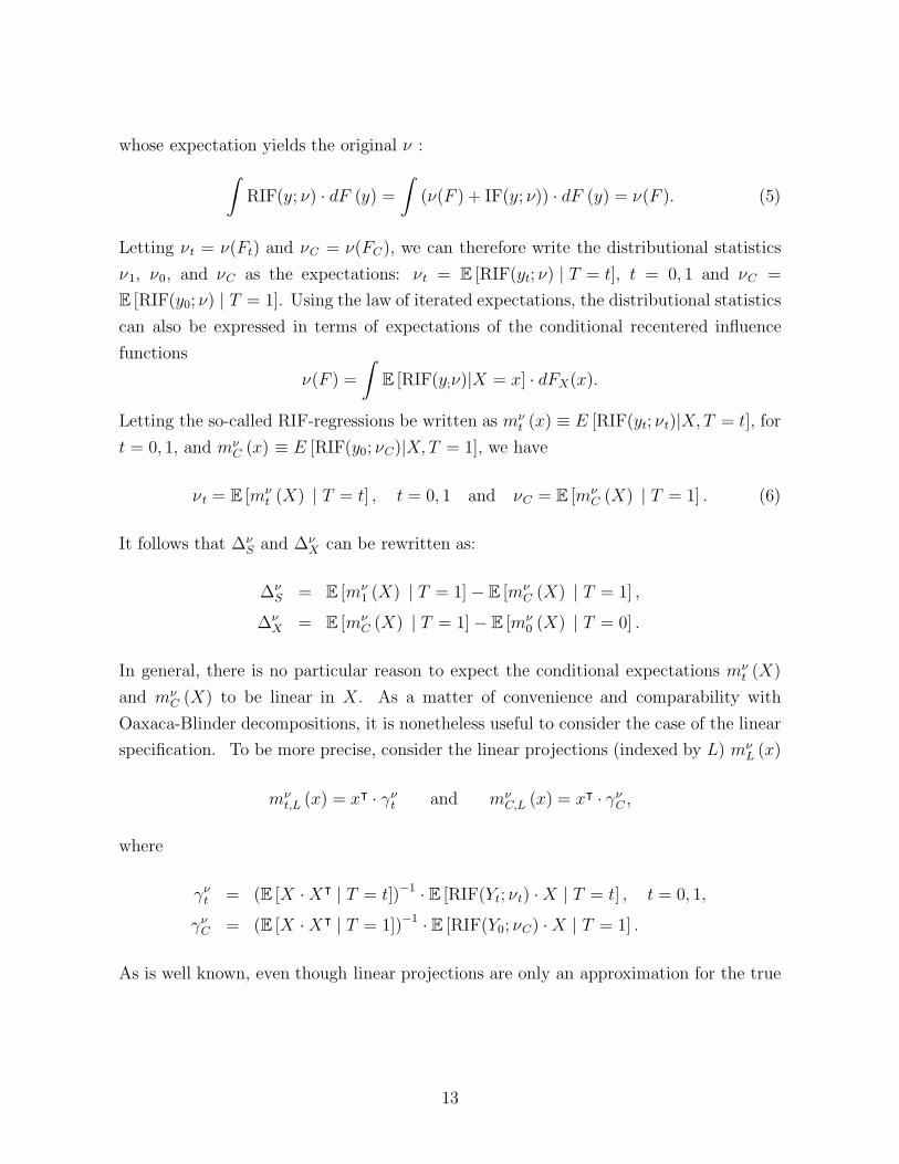
whose expectation yields the original ν :

∫RIF(y; ν) · dF (y) =

∫(ν(F ) + IF(y; ν)) · dF (y) = ν(F ). (5)

Letting νt = ν(Ft) and νC = ν(FC), we can therefore write the distributional statistics

ν1, ν0, and νC as the expectations: νt = E [RIF(yt; ν) | T = t], t = 0, 1 and νC =

E [RIF(y0; ν) | T = 1]. Using the law of iterated expectations, the distributional statistics

can also be expressed in terms of expectations of the conditional recentered influence

functions

ν(F ) =

∫E [RIF(y;ν)|X = x] · dFX(x).

Letting the so-called RIF-regressions be written as mνt (x) ≡ E [RIF(yt; νt)|X,T = t], for

t = 0, 1, and mνC (x) ≡ E [RIF(y0; νC)|X,T = 1], we have

ν t = E [mνt (X) | T = t] , t = 0, 1 and νC = E [mν

C (X) | T = 1] . (6)

It follows that ∆νS and ∆ν

X can be rewritten as:

∆νS = E [mν

1 (X) | T = 1] − E [mνC (X) | T = 1] ,

∆νX = E [mν

C (X) | T = 1] − E [mν0 (X) | T = 0] .

In general, there is no particular reason to expect the conditional expectations mνt (X)

and mνC (X) to be linear in X. As a matter of convenience and comparability with

Oaxaca-Blinder decompositions, it is nonetheless useful to consider the case of the linear

specification. To be more precise, consider the linear projections (indexed by L) mνL (x)

mνt,L (x) = xᵀ · γν

t and mνC,L (x) = xᵀ · γν

C ,

where

γνt = (E [X ·Xᵀ | T = t])−1 · E [RIF(Yt; νt) ·X | T = t] , t = 0, 1,

γνC = (E [X ·Xᵀ | T = 1])−1 · E [RIF(Y0; νC) ·X | T = 1] .

As is well known, even though linear projections are only an approximation for the true

13

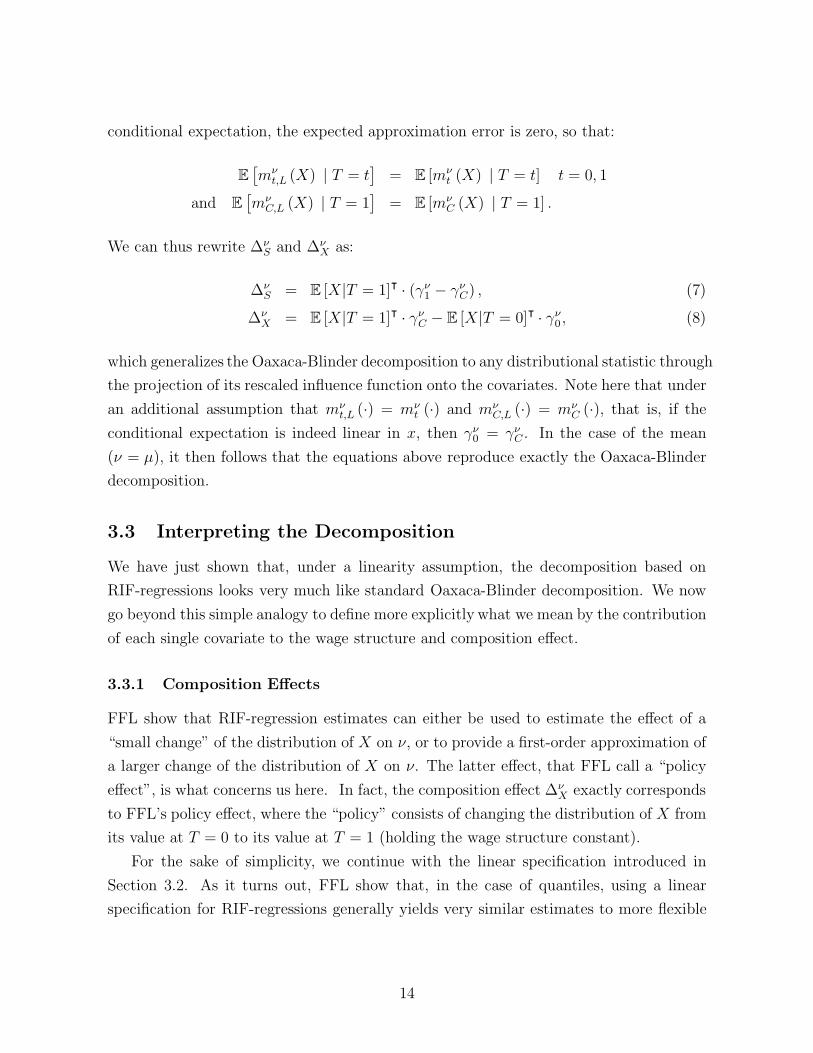
conditional expectation, the expected approximation error is zero, so that:

E[mν

t,L (X) | T = t]

= E [mνt (X) | T = t] t = 0, 1

and E[mν

C,L (X) | T = 1]

= E [mνC (X) | T = 1] .

We can thus rewrite ∆νS and ∆ν

X as:

∆νS = E [X|T = 1]ᵀ · (γν

1 − γνC) , (7)

∆νX = E [X|T = 1]ᵀ · γν

C − E [X|T = 0]ᵀ · γν0, (8)

which generalizes the Oaxaca-Blinder decomposition to any distributional statistic through

the projection of its rescaled influence function onto the covariates. Note here that under

an additional assumption that mνt,L (·) = mν

t (·) and mνC,L (·) = mν

C (·), that is, if the

conditional expectation is indeed linear in x, then γν0 = γν

C . In the case of the mean

(ν = µ), it then follows that the equations above reproduce exactly the Oaxaca-Blinder

decomposition.

3.3 Interpreting the Decomposition

We have just shown that, under a linearity assumption, the decomposition based on

RIF-regressions looks very much like standard Oaxaca-Blinder decomposition. We now

go beyond this simple analogy to define more explicitly what we mean by the contribution

of each single covariate to the wage structure and composition effect.

3.3.1 Composition Effects

FFL show that RIF-regression estimates can either be used to estimate the effect of a

“small change” of the distribution of X on ν, or to provide a first-order approximation of

a larger change of the distribution of X on ν. The latter effect, that FFL call a “policy

effect”, is what concerns us here. In fact, the composition effect ∆νX exactly corresponds

to FFL’s policy effect, where the “policy” consists of changing the distribution of X from

its value at T = 0 to its value at T = 1 (holding the wage structure constant).

For the sake of simplicity, we continue with the linear specification introduced in

Section 3.2. As it turns out, FFL show that, in the case of quantiles, using a linear

specification for RIF-regressions generally yields very similar estimates to more flexible

14

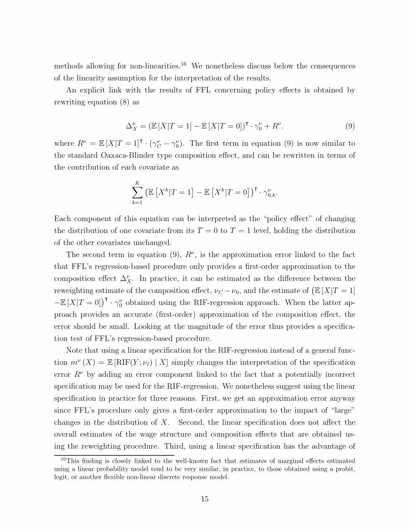
methods allowing for non-linearities.16 We nonetheless discuss below the consequences

of the linearity assumption for the interpretation of the results.

An explicit link with the results of FFL concerning policy effects is obtained by

rewriting equation (8) as

∆νX = (E [X|T = 1] − E [X|T = 0])ᵀ · γν

0 +Rν . (9)

where Rν = E [X|T = 1]ᵀ · (γνC − γν

0). The first term in equation (9) is now similar to

the standard Oaxaca-Blinder type composition effect, and can be rewritten in terms of

the contribution of each covariate as

K∑

k=1

(E[Xk|T = 1

]− E

[Xk|T = 0

])ᵀ · γν0,k.

Each component of this equation can be interpreted as the “policy effect” of changing

the distribution of one covariate from its T = 0 to T = 1 level, holding the distribution

of the other covariates unchanged.

The second term in equation (9), Rν , is the approximation error linked to the fact

that FFL’s regression-based procedure only provides a first-order approximation to the

composition effect ∆νX. In practice, it can be estimated as the difference between the

reweighting estimate of the composition effect, νC −ν0, and the estimate of(E [X|T = 1]

−E [X|T = 0])ᵀ · γν

0 obtained using the RIF-regression approach. When the latter ap-

proach provides an accurate (first-order) approximation of the composition effect, the

error should be small. Looking at the magnitude of the error thus provides a specifica-

tion test of FFL’s regression-based procedure.

Note that using a linear specification for the RIF-regression instead of a general func-

tion mν (X) = E [RIF(Y ; νt) | X] simply changes the interpretation of the specification

error Rν by adding an error component linked to the fact that a potentially incorrect

specification may be used for the RIF-regression. We nonetheless suggest using the linear

specification in practice for three reasons. First, we get an approximation error anyway

since FFL’s procedure only gives a first-order approximation to the impact of “large”

changes in the distribution of X. Second, the linear specification does not affect the

overall estimates of the wage structure and composition effects that are obtained us-

ing the reweighting procedure. Third, using a linear specification has the advantage of

16This finding is closely linked to the well-known fact that estimates of marginal effects estimatedusing a linear probability model tend to be very similar, in practice, to those obtained using a probit,logit, or another flexible non-linear discrete response model.

15

providing a much simpler interpretation of the decomposition, as in the Oaxaca-Blinder

decomposition. Our suggestion is thus to use the linear specification but also look at the

size of the specification error to make sure that the FFL approach provides an accurate

enough approximation for the problem at hand.

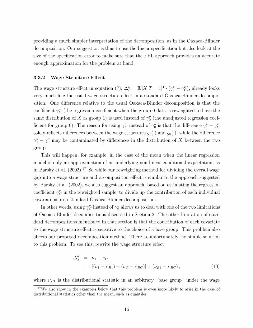
3.3.2 Wage Structure Effect

The wage structure effect in equation (7), ∆νS = E [X|T = 1]ᵀ · (γν

1 − γνC), already looks

very much like the usual wage structure effect in a standard Oaxaca-Blinder decompo-

sition. One difference relative to the usual Oaxaca-Blinder decomposition is that the

coefficient γνC (the regression coefficient when the group 0 data is reweighted to have the

same distribution of X as group 1) is used instead of γν0 (the unadjusted regression coef-

ficient for group 0). The reason for using γνC instead of γν

0 is that the difference γν1 − γν

C

solely reflects differences between the wage structures g1(·) and g0(·), while the difference

γν1 − γν

0 may be contaminated by differences in the distribution of X between the two

groups.

This will happen, for example, in the case of the mean when the linear regression

model is only an approximation of an underlying non-linear conditional expectation, as

in Barsky et al. (2002).17 So while our reweighting method for dividing the overall wage

gap into a wage structure and a composition effect is similar to the approach suggested

by Barsky et al. (2002), we also suggest an approach, based on estimating the regression

coefficient γνC in the reweighted sample, to divide up the contribution of each individual

covariate as in a standard Oaxaca-Blinder decomposition.

In other words, using γνC instead of γν

0 allows us to deal with one of the two limitations

of Oaxaca-Blinder decompositions discussed in Section 2. The other limitation of stan-

dard decompositions mentioned in that section is that the contribution of each covariate

to the wage structure effect is sensitive to the choice of a base group. This problem also

affects our proposed decomposition method. There is, unfortunately, no simple solution

to this problem. To see this, rewrite the wage structure effect

∆νS = ν1 − νC

= [(ν1 − νB1) − (νC − νBC)] + (νB1 − νBC) , (10)

where νB1 is the distributional statistic in an arbitrary “base group” under the wage

17We also show in the examples below that this problem is even more likely to arise in the case ofdistributional statistics other than the mean, such as quantiles.

16

structure g1(·, ·), while νBC is the distributional statistic for the same base group under

the wage structure g0(·, ·). The term ν1 − νB1 represents the “policy effect” of changing

the distribution of X from its value in the base group to its T = 1 value under the wage

structure g1(·, ·), while νC − νBC represents the corresponding policy effect under the

wage structure g0(·, ·). Since there is no dispersion in X in a base group of workers with

similar characteristics, switching to the actual distribution of X will typically result in

more wage dispersion. The overall wage structure effect is, thus, equal to the difference

in the dispersion enhancing effect under g1(·, ·) and g0(·, ·), respectively, plus a “residual”

difference in the distributional statistic in the base group, νB1−νBC. Unless this residual

change is invariant to the choice of the base group, the contribution of each covariate to

the wage structure will be sensitive to the choice of base group.

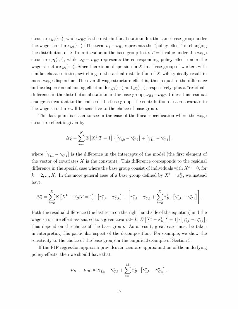
This last point is easier to see in the case of the linear specification where the wage

structure effect is given by

∆νS =

K∑

k=2

E[Xk|T = 1

]·[γν

1,k − γνC,k

]+[γν

1,1 − γνC,1

],

where[γ1,1 − γC,1

]is the difference in the intercepts of the model (the first element of

the vector of covariates X is the constant). This difference corresponds to the residual

difference in the special case where the base group consist of individuals with Xk = 0, for

k = 2, ...,K. In the more general case of a base group defined by Xk = xkB, we instead

have:

∆νS =

K∑

k=2

E[Xk − xk

B|T = 1]·[γν

1,k − γνC,k

]+

[γν

1,1 − γνC,1 +

K∑

k=2

xkB ·[γν

1,k − γνC,k

]].

Both the residual difference (the last term on the right hand side of the equation) and the

wage structure effect associated to a given covariate k, E[Xk − xk

B|T = 1]·[γν

1,k − γνC,k

],

thus depend on the choice of the base group. As a result, great care must be taken

in interpreting this particular aspect of the decomposition. For example, we show the

sensitivity to the choice of the base group in the empirical example of Section 5.

If the RIF-regression approach provides an accurate approximation of the underlying

policy effects, then we should have that

νB1 − νBC ≈ γν1,k − γν

C,k +M∑

k=1

xkB ·[γν

1,k − γνC,k

].

17

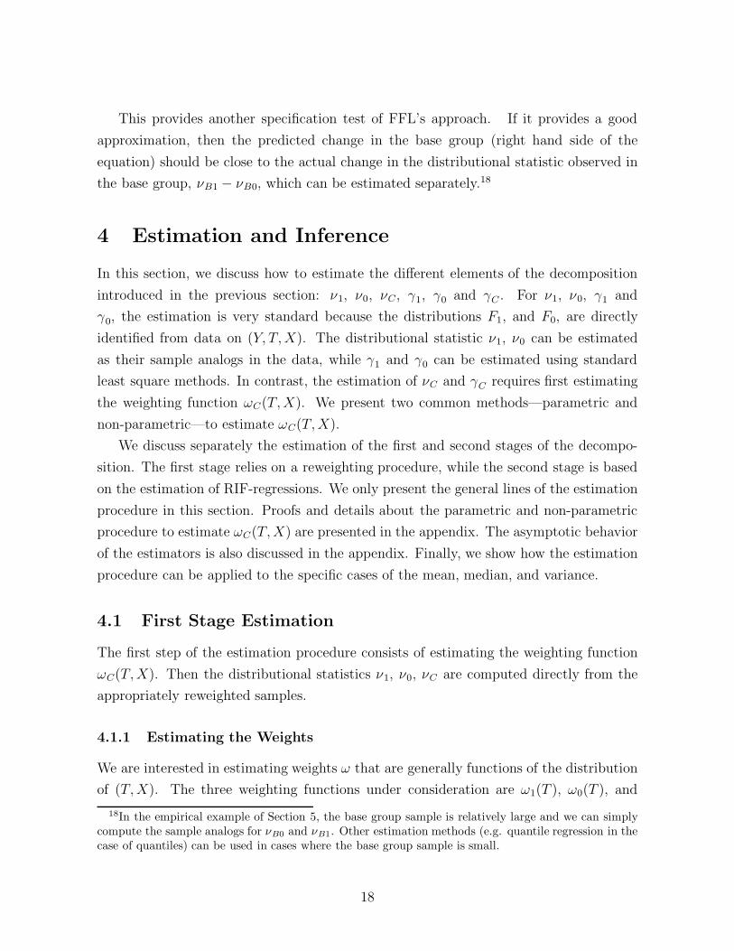
This provides another specification test of FFL’s approach. If it provides a good

approximation, then the predicted change in the base group (right hand side of the

equation) should be close to the actual change in the distributional statistic observed in

the base group, νB1 − νB0, which can be estimated separately.18

4 Estimation and Inference

In this section, we discuss how to estimate the different elements of the decomposition

introduced in the previous section: ν1, ν0, νC, γ1, γ0 and γC . For ν1, ν0, γ1 and

γ0, the estimation is very standard because the distributions F1, and F0, are directly

identified from data on (Y, T,X). The distributional statistic ν1, ν0 can be estimated

as their sample analogs in the data, while γ1 and γ0 can be estimated using standard

least square methods. In contrast, the estimation of νC and γC requires first estimating

the weighting function ωC(T,X). We present two common methods—parametric and

non-parametric—to estimate ωC(T,X).

We discuss separately the estimation of the first and second stages of the decompo-

sition. The first stage relies on a reweighting procedure, while the second stage is based

on the estimation of RIF-regressions. We only present the general lines of the estimation

procedure in this section. Proofs and details about the parametric and non-parametric

procedure to estimate ωC(T,X) are presented in the appendix. The asymptotic behavior

of the estimators is also discussed in the appendix. Finally, we show how the estimation

procedure can be applied to the specific cases of the mean, median, and variance.

4.1 First Stage Estimation

The first step of the estimation procedure consists of estimating the weighting function

ωC(T,X). Then the distributional statistics ν1, ν0, νC are computed directly from the

appropriately reweighted samples.

4.1.1 Estimating the Weights

We are interested in estimating weights ω that are generally functions of the distribution

of (T,X). The three weighting functions under consideration are ω1(T ), ω0(T ), and

18In the empirical example of Section 5, the base group sample is relatively large and we can simplycompute the sample analogs for νB0 and νB1. Other estimation methods (e.g. quantile regression in thecase of quantiles) can be used in cases where the base group sample is small.

18

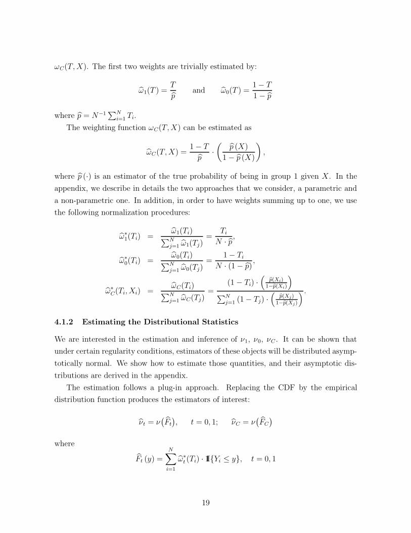
ωC(T,X). The first two weights are trivially estimated by:

ω1(T ) =T

pand ω0(T ) =

1 − T

1 − p

where p = N−1∑N

i=1 Ti.

The weighting function ωC(T,X) can be estimated as

ωC(T,X) =1 − T

p·(

p (X)

1 − p (X)

),

where p (·) is an estimator of the true probability of being in group 1 given X. In the

appendix, we describe in details the two approaches that we consider, a parametric and

a non-parametric one. In addition, in order to have weights summing up to one, we use

the following normalization procedures:

ω∗1(Ti) =

ω1(Ti)∑Nj=1 ω1(Tj)

=Ti

N · p ,

ω∗0(Ti) =

ω0(Ti)∑Nj=1 ω0(Tj)

=1 − Ti

N · (1 − p),

ω∗C(Ti,Xi) =

ωC(Ti)∑Nj=1 ωC(Tj)

=(1 − Ti) ·

(p(Xi)

1−p(Xi)

)

∑Nj=1 (1 − Tj) ·

(p(Xj)

1−p(Xj)

) .

4.1.2 Estimating the Distributional Statistics

We are interested in the estimation and inference of ν1, ν0, νC . It can be shown that

under certain regularity conditions, estimators of these objects will be distributed asymp-

totically normal. We show how to estimate those quantities, and their asymptotic dis-

tributions are derived in the appendix.

The estimation follows a plug-in approach. Replacing the CDF by the empirical

distribution function produces the estimators of interest:

νt = ν(Ft

), t = 0, 1; νC = ν

(FC

)

where

Ft (y) =N∑

i=1

ω∗t (Ti) · 1I{Yi ≤ y}, t = 0, 1

19

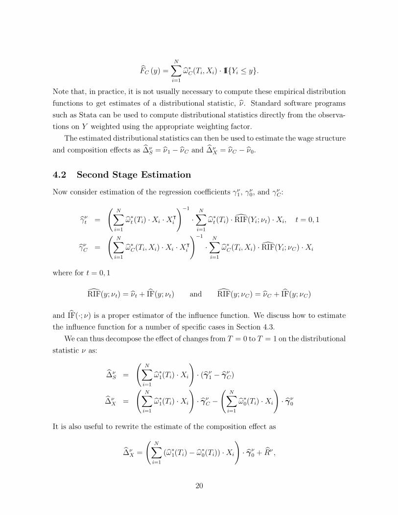
FC (y) =

N∑

i=1

ω∗C(Ti,Xi) · 1I{Yi ≤ y}.

Note that, in practice, it is not usually necessary to compute these empirical distribution

functions to get estimates of a distributional statistic, ν. Standard software programs

such as Stata can be used to compute distributional statistics directly from the observa-

tions on Y weighted using the appropriate weighting factor.

The estimated distributional statistics can then be used to estimate the wage structure

and composition effects as ∆νS = ν1 − νC and ∆ν

X = νC − ν0.

4.2 Second Stage Estimation

Now consider estimation of the regression coefficients γν1, γ

ν0, and γν

C:

γνt =

(N∑

i=1

ω∗t (Ti) ·Xi ·Xᵀ

i

)−1

·N∑

i=1

ω∗t (Ti) · RIF(Yi; νt) ·Xi, t = 0, 1

γνC =

(N∑

i=1

ω∗C(Ti,Xi) ·Xi ·Xᵀ

i

)−1

·N∑

i=1

ω∗C(Ti,Xi) · RIF(Yi; νC) ·Xi

where for t = 0, 1

RIF(y; νt) = νt + IF(y; νt) and RIF(y; νC) = νC + IF(y; νC)

and IF(·; ν) is a proper estimator of the influence function. We discuss how to estimate

the influence function for a number of specific cases in Section 4.3.

We can thus decompose the effect of changes from T = 0 to T = 1 on the distributional

statistic ν as:

∆νS =

(N∑

i=1

ω∗1(Ti) ·Xi

)· (γν

1 − γνC)

∆νX =

(N∑

i=1

ω∗1(Ti) ·Xi

)· γν

C −(

N∑

i=1

ω∗0(Ti) ·Xi

)· γν

0

It is also useful to rewrite the estimate of the composition effect as

∆νX =

(N∑

i=1

(ω∗1(Ti) − ω∗

0(Ti)) ·Xi

)· γν

0 + Rν ,

20

where Rν =(∑N

i=1 ω∗1(Ti) ·Xi

)·(γν

1 − γνC) is the approximation error discussed in Section

3.1. This generalizes the Oaxaca-Blinder decomposition to any distributional statistic,

including the variance or the Gini coefficient.

4.3 Examples

We now turn to the specific cases of the mean, the median, and the variance to illustrate

how the different elements of the decomposition can be computed in these specific cases.

4.4 The Mean

The standard Oaxaca-Blinder decomposition presented in Section 2 is only valid under

the assumption that the underlying “structural” model is linear

Yti = gt(Xi, εti) = Xiβt + εti, if t = 0, 1 (11)

and under the zero conditional mean assumption E(εti|Xi, T ) = 0. In contrast, our two-

stage decomposition neither requires linearity nor the zero conditional mean assumption

(ignorability is sufficient).

In a first stage, we compute the means by reweighting

µt = N−1N∑

i=1

ωt(Ti) · Yi, t = 0, 1 and µC = N−1N∑

i=1

ωC(Ti,Xi) · Yi, (12)

to estimate the wage gaps

∆µO = µ1 − µ0; ∆µ

S = µ1 − µC ; and ∆µX = µC − µ0. (13)

Note, in particular, that we can compute the counterfactual µC without any assumptions

on the functional form of gt(·).In the second stage, we further decompose these expressions into components at-

tributable to each covariate by estimating OLS regressions of the RIF on X for the

T = 0, 1 samples, and the T = 0 sample reweighted to have the same distribution of X

as in T = 1.

As is well known, the influence function of the mean at point y is its deviation from the

mean and, therefore, the rescaled influence function of the mean is simply the observation

21

itself

IF(y;µ) = limε→0

[(1 − ε) · µ+ ε · y − µ]

ε= y − µ, (14)

RIF(y;µ) = IF(y;µ) + µ = y. (15)

As a result, the RIF-regression coefficients in the case of the mean are identical to

standard regression coefficients of Y on X used in the Oaxaca-Blinder decomposition (βt

above), and we have

γµt =

(N∑

i=1

ωt(Ti)XiXi′

)−1

·N∑

i=1

ωt(Ti)XiYi, t = 0, 1

γµC =

(N∑

i=1

ωC(Ti,Xi)XiXi′

)−1

·N∑

i=1

ωC(Ti,Xi)XiYi,

where γµt = βt, and

∆µS = E [X,T = 1]ᵀ · (γµ

1 − γµC) , (16)

∆µX = (E [X|T = 1] − E [X|T = 0])ᵀ · γµ

0 +Rµ. (17)

When the linearity and zero conditional mean assumption of the Oaxaca-Blinder

decomposition are satisfied, it follows that γµC = γµ

0 and Rµ = 0. Our decomposition is

then identical to the Oaxaca-Blinder decomposition. But when these conditions are not

satisfied the two decompositions are different.

4.5 The Median

Quantiles are another set of distributional measures that have been used for the decompo-

sition of wage distributions. In decompositions of the gender wage gap, they are used to

address issues such as glass ceilings and sticky floors. In the example below, they will be

used, for example, to differentiate the impact of unions in the middle of the distribution

from its impact in the tails (Chamberlain, 1994).

The τ -th quantile of the distribution F is defined as the functional, Q(F, τ) =

inf{y|F (y) ≥ τ}, or as qτ for short, and its influence function is:

IF(y; qτ) =τ − 1I {y ≤ qτ}

fY (qτ). (18)

22

The rescaled influence function of the τ th quantile is RIF(y; qτ) = qτ + IF(y; qτ) = qτ +

(τ − 1I{y ≤ qτ})/fY (qτ).

A leading example of an estimator in this class is the median. The influence function

of the median, ψme, is

IF(y;me) =(1/2 − 1I{y ≤ me})

f(me),

and the rescaled influence function is RIF(y;me) = me+ (1/2 − 1I{y ≤ me})/f(me).

The decomposition of the median proceeds along the same steps as in the case of the

mean. In the first stage, the estimates of met, t = 0, 1 and meC are obtained by reweight-

ing as met = arg minq

∑Ni=1 ωt(Ti)· |Yi − q|, t = 0, 1 and meC = arg minq

∑Ni=1 ωC(Ti)·

|Yi − q|. Note that these estimates can simply be computed using standard software

packages with the appropriate weighting factor.

The estimators for the gaps are computed as:

∆meO = me1 − me0; ∆me

S = me1 − meC and ∆meX = meC − me0. (19)

In the second stage, we estimate the linear RIF-regressions. First, the rescaled influ-

ence function is computed for each observation by plugging the sample estimate of the

quantile, qτ , and estimating the density at the sample quantile, f (qτ). For example,

for the median of Y1|T = 1, we would use RIF(y;me1) = me1 +(f1 (me1)

)−1

· (1/2 −1I{y ≤ me1}) where f1 (·) is a consistent estimator for the density of Y1|T = 1, f1 (·). For

example, kernel methods can be used to estimate the density (see FFL for more detail).

The RIF-regressions are then estimated by replacing the usual dependent variable,

Y , by the estimated value of RIF(y;me1). Standard software packages can be used to do

so. The resulting regression coefficients are

γmet =

(N∑

i=1

ωt(Ti)XiXi′

)−1

·N∑

i=1

ωt(Ti)XiRIF(Yi;met), t = 0, 1, (20)

γmeC =

(N∑

i=1

ωC(Ti,Xi)XiXi′

)−1

·N∑

i=1

ωC(Ti,Xi)XiRIF(Yi;meC). (21)

Similarly to the case of the mean, we get:

∆meS = E [X,T = 1]ᵀ · (γme

1 − γmeC ) , (22)

∆meX = (E [X|T = 1] − E [X|T = 0])ᵀ · γme

0 + Rme, (23)

23

where Rme = E [X|T = 1]ᵀ · (γmeC − γme

0 ).

4.6 The Variance

There are other applications where it is useful to decompose the impact of covariates on

the variance of the distributions of wages. Examples include the compression effect of

unions and of public sector wage setting.

As before, the estimators of the gaps can be computed as:

∆σ2

O = σ21 − σ2

0; ∆σ2

S = σ21 − σ2

C and ∆σ2

X = σ2C − σ2

0, (24)

using the reweighting scheme σ2t = N−1

∑Ni=1 ωt(Ti) · (Yi − µt)

2, t = 0, 1, and σ2C =

N−1∑N

i=1 ωC(Ti) · (Yi − µC)2. The influence function of the variance is well-known to be

IF(y;σ2) =

(y −

∫z · dFY (z)

)2

− σ2, (25)

and the rescaled influence function is the first term of this expression RIF(y;σ2) =(y −

∫z · dFY (z)

)2= (Y − µ)2.

The decomposition in terms of individual covariates, such as union coverage, follows

by replacing RIF(·;me) by RIF(·;σ2) in equations (20), (21), (22), and (23).

4.7 The Gini

Finally, another popular measure of wage inequality is the Gini. Recall that Gini coeffi-

cient is defined as

νGC(FY ) = 1 − 2µ−1R(FY ) (26)

where R(FY ) =∫ 1

0GL(p;FY )dp with p(y) = FY (y) and where GL(p;FY ) the generalized

Lorenz ordinate of FY is given by GL(p;FY ) =∫ F−1(p)

−∞ z dFY (z). The generalized Lorenz

curve tracks the cumulative total of y divided by total population size against the cu-

mulative distribution function and the generalized Lorenz ordinate can be interpreted as

the proportion of earnings going to the 100p% lowest earners.

As shown in Monti (1991), the influence function of the Gini coefficient is

IF(y; νGC ) = A2(FY ) +B2(FY )y + C2(y;FY ) (27)

24

where

A2(FY ) = 2µ−1R(FY )

B2(FY ) = 2µ−2R(FY )

C2(y;FY ) = −2µ−1 [y [1 − p(y)] +GL (p(y);FY )]

with R(FY ) and GL(p(y);FY ) as defined in equation (26). Thus the recentered influence

function of the Gini is simply

RIF(y; νGC) = 1 +B2(FY )y + C2(y;FY ) (28)

In estimation, the GL coordinates are computed using a series of discrete data points

y1, . . . yN , where observations have been ordered so that y1 ≤ y2 ≤ . . . ≤ yN , so that

pt(yi) =

∑ij=1 ωt(Tj)∑Nj=1 ωt(Tj)

, GLt(p(yi)) =

∑ij=1 ωt(Tj) · Yj∑N

j=1 ωt(Tj)t = 0, 1

pC(yi) =

∑ij=1 ωC(Tj)∑Nj=1 ωC(Tj)

, GLC(p(yi)) =

∑ij=1 ωC(Tj) · Yj∑N

j=1 ωC(Tj)

where the numerators are the sum up the i ordered values of Y . The R(Ft), t = 0, 1 and

R(FC) are obtained by numerical integration of GLt(p(yi)) over pt(yi), and of GLC(p(yi))

over pC(yi).19 The estimates of νGC(Ft), t = 0, 1 and νGC(FC) are obtained by subtituting

R(Ft) and R(FC), as well as µt and µC , into equation (26). We can then compute the

gaps for the changes in the Gini coefficient as in equation(24).

Similar substitutions into equation (28) allows the estimation of RIF(y; νGCt ), t = 0, 1

and RIF(y; νGCC ). As before, the decomposition in terms of individual covariates, follows

by replacing RIF(·;me) by RIF(·; νGC) in equations (20), (21), (22), and (23).

5 Empirical Application: Changes in Male Wage In-

equality between 1988 and 2005

It is well known that wage inequality increased sharply in the United States over the

last 30 years. Using various distributional methods, Juhn, Murphy and Pierce (1993)

19In pratice, we simply use STATA integ command.

25

and DiNardo, Fortin and Lemieux (1996) show that inequality expanded all through the

wage distribution during the 1980s. In particular, both the “90-50 gap” (the difference

between the 90th and the 50th quantile of log wages) and the “50-10 gap” increased

during this period.

Since the late 1980s, however, changes in inequality have increasingly been concen-

trated in the top end of the wage distribution. In fact, Autor, Katz and Kearney (2006)

show that while the 90-50 gap kept expanding over the last 15 years, the 50-10 gap

declined during the same period. They refer to these recent changes as an increased po-

larization of the labor market. An obvious question is why wage dispersion has changed

so differently at different points of the distribution. Autor, Katz and Kearney (2006)

suggest that technological change is a possible answer, provided that computerization re-

sulted in a decline in the demand for skilled but “routine” tasks that used to be performed

by workers around the middle of the wage distribution.20

Lemieux (2007) reviews possible explanations for the increased polarization in the

labor market, including the technological-based explanation of Autor, Katz and Kearney.

He suggests that if this explanation is an important one, then changes in relative wages

by occupation, i.e. the contribution of occupations to the wage structure effect, should

play an important role in changes in the wage distribution. Furthermore, since it is well

know that education wage differentials kept expanding during after the late 1980s (e.g.

Deschenes 2004), the contribution of education to the wage structure effect is another

leading explanation for inequality changes over this period.

Existing studies also show that composition effects played an important role over the

1988-2005 period. Lemieux (2006b) shows that all the growth in residual inequality over

this period is due to composition effects linked to the fact that the workforce became older

and more educated, two factors associated with more wage dispersion. Furthermore,

Lemieux (2007) argues that de-unionization, another composition effect the way it is

defined in this paper, still contributed to the changes in the wage distribution over this

period.

These various explanations can all be categorized in terms of the respective contribu-

tions of various sets of factors (occupations, unions, education, experience, etc.) to either

wage structure or composition effects. This makes the decomposition method proposed

in this paper ideally suited for estimating the contribution of each of these possible ex-

20This technological change explanation was first suggested by Autor, Levy, and Murnane (2003). Italso implies that the wages of both skilled (e.g. doctors) and unskilled (e.g. truck drivers) non-routinejobs, at the top and low end of the wage distribution, increased relative to those of “routine” workers inthe middle of the wage distribution.

26

planations to changes in the wage distribution. Applying our method to this issue fills

an important gap in the literature, since no existing study has systematically attempted

to estimate the contribution of each of the aforementioned factors to recent changes in

the U.S. wage distribution.21

Our empirical analysis is based on data for men from the 1988-90 and 2003-05 Outgo-

ing Rotation Group (ORG) Supplements of the Current Population Survey. The data files

were processed as in Lemieux (2006b) who provides detailed information on the relevant

data issues. The wage measure used is an hourly wage measure computed by dividing

earnings by hours of work for workers not paid by the hour. For workers paid by the

hour, we use a direct measure of the hourly wage rate. In light of the above discussion,

the key set of covariates on which we focus are education (six education groups), poten-

tial experience (nine groups), union coverage, and occupation (17 categories). We also

include controls for industry (14 categories), marital status, and race in all the estimated

models. The sample means for all these variables are provided in Table A1.22

To capture the rich pattern of change in the wage distribution between 1988-1990

and 2003-05, we decompose the changes in 19 different wage quantiles (from the 5th

to the 95th quantile) equally spread over the whole wage distribution. This enables

us to see whether different factors have different impacts at different points of the wage

distribution. Using this flexible approach, as opposed to summary measures of inequality

like the Gini coefficient or the variance of log wages, is important since wage dispersion

changes very differently at different points of the distribution during this period.

5.1 RIF-Regressions

Before showing the decomposition results, we first present some estimates from the RIF-

regressions for the different wage quantiles, and for the variance of log wages and the

Gini coefficient. From equation (18), we compute IF(yi; qτ) for each observation using the

sample estimate of qτ , and the kernel density estimate of f (qτ) using the Epanechnikov

kernel and a bandwidth of 0.06. In addition to the reweighting factors discussed in

Sections 3 and 4, we also use CPS sample weights throughout the empirical analysis. In

practice, this means that we multiply the relevant reweighting factor with CPS sample

21Autor, Katz and Kearney (2005) use the Machado and Mata (2005) method to decompose changesat each quantile into a “price” (wage structure) and “quantity” (composition) effect. They do not furtherconsider, however, the contribution of each individual covariate to the wage structure effect, except forseparating the contribution of (all) covariates from the residual change in inequality. See also Lemieux(2002) for a similar decomposition based on a reweighting procedure.

22Table A2 gives the details of the occupation and industry categories used.

27

weight.

The RIF-regression coefficients for the 10th, 50th, and 90th quantiles in 1988-90 and

2003-05, along with their (robust) standard errors are reported in Table 1. The RIF-

regression coefficients for the variance and the Gini are reported in Table 2. Detailed

estimates for each of the 19 quantiles from the 5th to the 95th are also reported in Figure

1. Both Table 1 and the first panel of Figure 1 show that the effect of the union status

across the different quantiles is highly non-monotonic. In both 1988-90 and 2003-2005,

the effect first increases up to around the median, and then declines. The union effect

even turns negative for the 90th and 95th quantiles. On the whole, unions tend to reduce

wage inequality, since the wage effect tends to be larger for lower than higher quantiles

of the wage distribution. As shown by the RIF-regressions for the more global measures

of inequality–the variance of log wages and the Gini coefficient–displayed in Table 2, the

effect of unions on these measures is negative, although the magnitude of that effect has

decreased over time. This is consistent with the well-known result (e.g. Freeman, 1980)

that unions tend to reduce the variance of log wages for men.

More importantly, the results also indicate that unions increase inequality in the

lower end of the distribution, but decrease inequality even more in the higher end of

the distribution. For example, the estimates in Table 1 for 1988-90 imply that a 10

percent increase in the unionization rate would increase the 50-10 gap by 0.024, but

decrease the 90-50 gap by 0.043.23 As we will see later in the decomposition results, this

means that the continuing decline in the rate of unionization can account for some of the

“polarization” of the labor market (decrease in inequality at the low-end, but increase in

inequality at the top end).

The results for unions also illustrate an important feature of RIF regressions for quan-

tiles, namely that they capture the effect of covariates on both between- and within-group

component of wage dispersion. As made clear in the numerical exercise below, the within-

effect of unions on log wages across quantiles is negatively sloped (reduces inequality)

while the between effect is positively sloped (increases inequality). The different relative

strength of between and within effects at different quantiles explain the inverse U-shaped

effect of unions. This is in sharp contrast with the effect of unions found in conditional

quantile regressions which capture only within-group effects and is thus only negatively

sloped.

23These numbers are obtained by multiplying the change in the unionization rate (0.1) by the differencebetween the effects at the 50th and 10th quantiles (0.394-0.158=0.236), and at the 90th and 50th quantiles(–0.053-0.394=-0.429).

28

The RIF-regression estimates in Table 1 for other covariates also capture between-

and within-group effects, just as in the case of unions. Consider, for instance, the case

of college education. Table 1 and Figure 1 show that the effect of college increases

monotonically as a function of percentiles. In other words, increasing the fraction of the

workforce with a college degree has a larger impact on higher than lower quantiles. The

reason why the effect is monotonic is that education increases both the level and the

dispersion of wages (see, e.g. Lemieux, 2006a). As a result, both the within- and the

between-group effects go in the same direction of increasing inequality. Similarly, the

effect of experience also tends to be monotonic as experience has a positive impact on

both the level and the dispersion of wages.

Another clear pattern that emerges in Figure 1 is that, for most inequality enhancing

covariates, i.e. those with a positively sloped curve, the inequality enhancing effect

increases over time. In particular, the slopes for high levels of education (college graduates

and post-graduates) and high wage occupations (financial sales, doctors and lawyers)

become clearly steeper over time. This suggests that these covariates make a positive

contribution to the wage structure effect.

There are some changes in the contribution of occupations and industries that are

consistent with technological change, however these changes are dwarfed the ones asso-

ciated with other explanations. For example, there are some increases in the returns to

engineering and computer occupations, and in high-tech service industries, but these are

extremely small in comparison to the increases in the insurance, real estate and financial

sales occupations. There are increases in the penalties to routine production occupa-

tions in the upper-middle of wage distribution and at the lower end of the distribution.

There are also decreases in the penalties to some low skilled non-routine occupations

and associated industries, such as service occupations and truck driving and the retail

industry, but these changes in relatively small. In summary, the changes in the rewards

and penalties associated with occupations and industries are likely too modest to account

for a significant share of the changes in the wage structure between 1988 and 2005.

To help interpret the results, we now present a simulation exercise to illustrate how

the between and within-group effects work in the case of union before returning to the

main decomposition results.

5.1.1 Numerical Example of Between- and Within-Group Effects of Unions

It is well known in the literature that unions have an inequality enhancing effect because

they increase the conditional mean of wages, which creates a wedge between otherwise

29

comparable union and non-union workers. This between-group effect is offset, however,

by the within-group effect linked to the fact that unions reduce the conditional dispersion

of wages. In the case of the variance, it is easy to write down an analytical expression

for the between- and within-group effects (see, for example, Card, Lemieux, and Riddell,

2004) and see under which conditions one effect dominates the other. It is much harder

to know, however, whether the between- or the within-group effect tends to dominate at

different points of the wage distribution.

We illustrate the effect of unions at each percentile of the wage distribution using a

simple simulation exercise presented in Figure A1. We assume that union and non-union

(log) wages are normally distributed with standard deviations of 0.2 and 0.4, respectively.

The union wage gap is set to 0.3 (mean log wages of 2.3 and 2.0 in the union and non-

union sectors). The overall density of wages is obtained by adding the densities from the

union and non-union sectors, assuming a 25 percent unionization rate. Since no other

covariates are included in the example, the “effect” of unions at each percentile of the

overall distribution is simply the difference between the average value of the recentered

influence function for union and non-union workers.24

Panel A of Figure A1 shows the between-group effect at each percentile. The effect is

obtained by setting the standard deviation in the union sector at 0.4 (same as non-union)

to isolate the impact linked to the fact that the mean log wage is 0.3 larger in the union

than non-union sector. Since the curve in Panel A is positively sloped, the between-group

effect increases inequality. In contrast, the within-group effect of unions illustrated in

Panel B reduces inequality since the curve is negatively sloped instead. This effect is

obtained by setting mean log wages in both the union and non-union sector to 2.0, to

isolate the impact of the wage compression effect of unions.

The total effect of unions that includes both the between- and within-group com-

ponents is shown in Panel C of the figure. The effect looks qualitatively similar to the

actual union effect estimates reported in Figure 1. The effect of unions first becomes

larger in the lower half of the distribution, but turns around and becomes negative by

the time we reach the 90th percentile. Roughly speaking, we see that the inequality

enhancing between-group effect dominates in the lower end of the distribution, while the

24The effect is equal to [FN (qτ ) − FU (qτ )]/f (qτ ), where f (qτ ) = U · fU (qτ ) + (1 − U ) · fN (qτ ),U is the unionization rate (0.25 here), and fs (·) and Fs (·) are the normal PDF and CDF in theunion (s = U ) and non-union (s = N ) sectors. This result can also be directly obtained by notingthat since the overall CDF is F (qτ ) = U · FU (qτ ) + (1 − U ) · FN (qτ ), the total differential (holdingτ = F (qτ ) constant) is 0 = −[FN (qτ ) − FU (qτ )] · dU + [U · fU (qτ ) + (1 − U ) · fN (qτ )] · dqτ , so thatdqτ /dU = [FN (qτ ) − FU (qτ )]/f (qτ ) since f (qτ ) = U · fU (qτ ) + (1 − U ) · fN (qτ ).

30

inequality reducing within-group effect dominates in the upper end of the distribution.

Note that unlike the case of the variance where the between- and within-group effects

add-up exactly, these two effects do not directly add-up in the case of quantiles because

of the underlying non-linear structure of the model.

The last panel of Figure A1 provides a different type of intuition for the inverse U-

shaped nature of the effect of unions. The panel shows the CDF of wages for union,

non-union, and all (25 percent union, 75 percent non-union) workers. The CDF for all

workers, F (·), is simply the weighted average of the CDF for union, FU (·), and non-

union, FN (·), workers:

F (qτ) = U · FU (qτ) + (1 − U ) · FN (qτ) .

Since there are very few union workers below a log wage of about 2 in the example,

the overall CDF in that part of the distribution is essentially just the non-union CDF,

FN (qτ), times the constant 1−U . The higher is the unionization rate, the lower is 1−U ,

and the flatter is (1 − U ) · FN (qτ). Panel D indeed shows that the CDF for all workers

below about 2.0 (the dotted line) is flatter than the non-union CDF. The horizontal

distance between the CDF with (dotted line) and without unions (the non-union CDF)

thus increases as a function of percentiles in this part of the distribution. Since this

horizontal distance corresponds to a wage impact of unions for a given percentile, this

means that this wage effect first increases as a function of percentiles, just like in Panel

C. But once we get above 2.0, the horizontal distance between the CDF curves for non-

union and all workers starts decreasing as we hit the mass of union workers who have

more evenly distributed wages (i.e. a steeper CDF). This accounts for the reversal of the

union effect shown in Panel C.

5.2 Decomposition Results

The results of the decomposition are presented in Figure 2. Table 3 also summarizes

the results for the standard measure of top-end (90-50 gap) and low-end (50-10) wage

inequality, as well as for the variance of log wages and the Gini coefficient. The base

group used in the decomposition consists of non-union, white, and married men with

some college education, and 20 to 24 years of potential experience.25 The covariates used

in the RIF-regression models are those discussed above and listed in Table A1. A richer

25We also present an alternative set of results in Figure A2 when high school education is used insteadof some college as the base group.

31

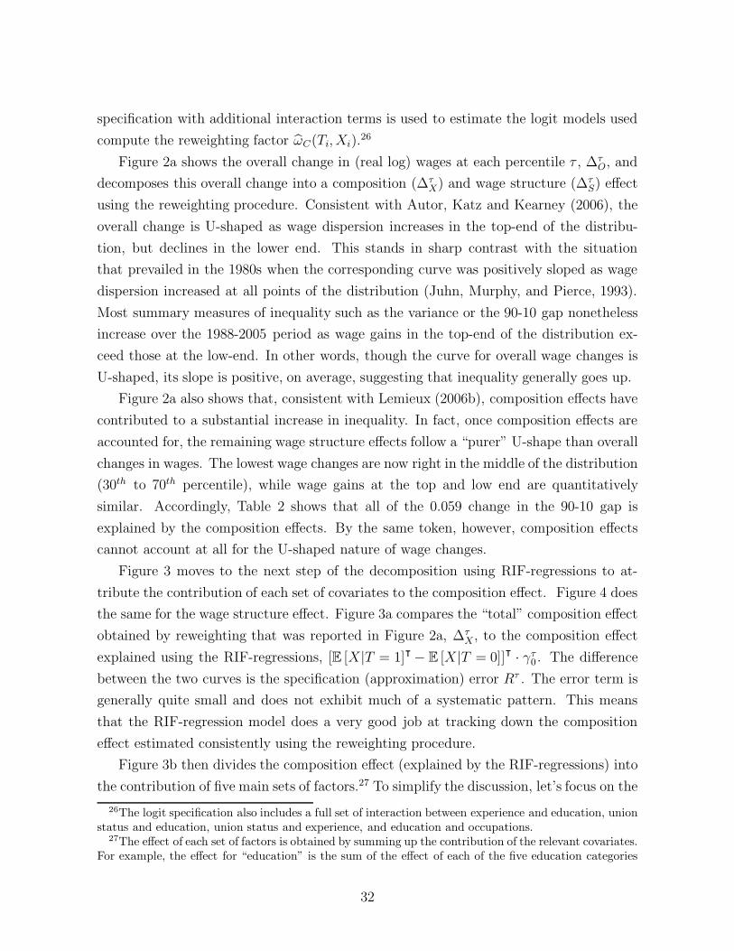
specification with additional interaction terms is used to estimate the logit models used

compute the reweighting factor ωC(Ti,Xi).26

Figure 2a shows the overall change in (real log) wages at each percentile τ , ∆τO, and

decomposes this overall change into a composition (∆τX) and wage structure (∆τ

S) effect

using the reweighting procedure. Consistent with Autor, Katz and Kearney (2006), the

overall change is U-shaped as wage dispersion increases in the top-end of the distribu-

tion, but declines in the lower end. This stands in sharp contrast with the situation

that prevailed in the 1980s when the corresponding curve was positively sloped as wage

dispersion increased at all points of the distribution (Juhn, Murphy, and Pierce, 1993).

Most summary measures of inequality such as the variance or the 90-10 gap nonetheless

increase over the 1988-2005 period as wage gains in the top-end of the distribution ex-

ceed those at the low-end. In other words, though the curve for overall wage changes is

U-shaped, its slope is positive, on average, suggesting that inequality generally goes up.

Figure 2a also shows that, consistent with Lemieux (2006b), composition effects have

contributed to a substantial increase in inequality. In fact, once composition effects are

accounted for, the remaining wage structure effects follow a “purer” U-shape than overall

changes in wages. The lowest wage changes are now right in the middle of the distribution

(30th to 70th percentile), while wage gains at the top and low end are quantitatively

similar. Accordingly, Table 2 shows that all of the 0.059 change in the 90-10 gap is

explained by the composition effects. By the same token, however, composition effects

cannot account at all for the U-shaped nature of wage changes.

Figure 3 moves to the next step of the decomposition using RIF-regressions to at-

tribute the contribution of each set of covariates to the composition effect. Figure 4 does

the same for the wage structure effect. Figure 3a compares the “total” composition effect

obtained by reweighting that was reported in Figure 2a, ∆τX, to the composition effect

explained using the RIF-regressions, [E [X|T = 1]ᵀ − E [X|T = 0]]ᵀ · γτ

0. The difference

between the two curves is the specification (approximation) error Rτ . The error term is

generally quite small and does not exhibit much of a systematic pattern. This means

that the RIF-regression model does a very good job at tracking down the composition

effect estimated consistently using the reweighting procedure.

Figure 3b then divides the composition effect (explained by the RIF-regressions) into

the contribution of five main sets of factors.27 To simplify the discussion, let’s focus on the

26The logit specification also includes a full set of interaction between experience and education, unionstatus and education, union status and experience, and education and occupations.

27The effect of each set of factors is obtained by summing up the contribution of the relevant covariates.For example, the effect for “education” is the sum of the effect of each of the five education categories

32

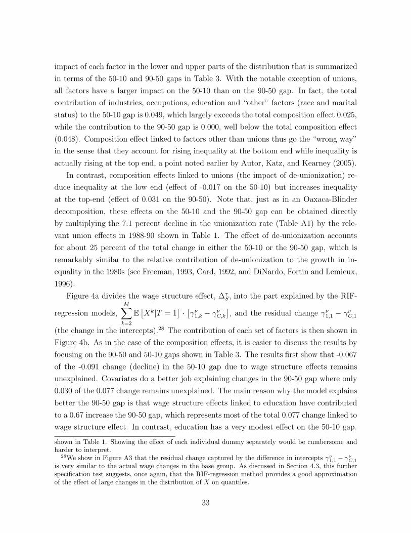
impact of each factor in the lower and upper parts of the distribution that is summarized

in terms of the 50-10 and 90-50 gaps in Table 3. With the notable exception of unions,

all factors have a larger impact on the 50-10 than on the 90-50 gap. In fact, the total

contribution of industries, occupations, education and “other” factors (race and marital

status) to the 50-10 gap is 0.049, which largely exceeds the total composition effect 0.025,

while the contribution to the 90-50 gap is 0.000, well below the total composition effect

(0.048). Composition effect linked to factors other than unions thus go the “wrong way”

in the sense that they account for rising inequality at the bottom end while inequality is

actually rising at the top end, a point noted earlier by Autor, Katz, and Kearney (2005).

In contrast, composition effects linked to unions (the impact of de-unionization) re-

duce inequality at the low end (effect of -0.017 on the 50-10) but increases inequality

at the top-end (effect of 0.031 on the 90-50). Note that, just as in an Oaxaca-Blinder

decomposition, these effects on the 50-10 and the 90-50 gap can be obtained directly

by multiplying the 7.1 percent decline in the unionization rate (Table A1) by the rele-

vant union effects in 1988-90 shown in Table 1. The effect of de-unionization accounts

for about 25 percent of the total change in either the 50-10 or the 90-50 gap, which is

remarkably similar to the relative contribution of de-unionization to the growth in in-

equality in the 1980s (see Freeman, 1993, Card, 1992, and DiNardo, Fortin and Lemieux,

1996).

Figure 4a divides the wage structure effect, ∆τS, into the part explained by the RIF-

regression models,M∑

k=2

E[Xk|T = 1

]·[γν

1,k − γνC,k

], and the residual change γν

1,1 − γνC,1

(the change in the intercepts).28 The contribution of each set of factors is then shown in

Figure 4b. As in the case of the composition effects, it is easier to discuss the results by

focusing on the 90-50 and 50-10 gaps shown in Table 3. The results first show that -0.067

of the -0.091 change (decline) in the 50-10 gap due to wage structure effects remains

unexplained. Covariates do a better job explaining changes in the 90-50 gap where only

0.030 of the 0.077 change remains unexplained. The main reason why the model explains

better the 90-50 gap is that wage structure effects linked to education have contributed

to a 0.67 increase the 90-50 gap, which represents most of the total 0.077 change linked to

wage structure effect. In contrast, education has a very modest effect on the 50-10 gap.

shown in Table 1. Showing the effect of each individual dummy separately would be cumbersome andharder to interpret.

28We show in Figure A3 that the residual change captured by the difference in intercepts γν1,1 − γν

C,1

is very similar to the actual wage changes in the base group. As discussed in Section 4.3, this furtherspecification test suggests, once again, that the RIF-regression method provides a good approximationof the effect of large changes in the distribution of X on quantiles.

33

These findings confirm Lemieux (2006a)’s conjecture that the large increase in the return

to post-secondary education has contributed to a convexification of the wage distribution.

Compared to education, the impact of most other factors is relatively modest. For

example, wage structure effects linked to occupations account for some of the decline

in inequality at the low-end, but for little of the growth at the top end. This suggests

that technological changes that reduce wages in routine occupations but increase wages

in non-routine occupation have had a modest impact on the wage structure between

1988-2005, once education is controlled for.

Finally, the total effect of each covariate (wage structure plus composition effect) is

reported in Figure 2b and in the bottom panel of Table 3. Unions and education are

clearly the two dominant explanations for recent changes in the wage distribution. In

both cases, the total effect of these factors on the 90-50 gap is about 0.04-0.05 larger

than the effect on the 50-10 gap. This goes a substantial way towards explaining the

polarization of the labor market, i.e. why the 90-50 gap increased by 0.19 more than the

50-10 gap.

6 Conclusion

We propose a two-stage method to decompose changes in the distribution of wages (or

other outcome variables). In stage 1, distributional changes are divided into a wage struc-

ture effect and a composition effect using a reweighting method. In stage 2, these two

components are further divided into the contribution of each individual covariate using a

novel influence function regression technique introduced by Firpo, Fortin, and Lemieux

(2006). This two-stage procedure generalizes the popular Oaxaca-Blinder decomposi-

tion method by extending the decomposition to any distributional measure (besides the

mean), and allowing for a much more flexible wage setting model. Other procedures have

been suggested for performing part of this decomposition for distributional parameters

besides the means. One important advantage of our procedure is that it is easy to use

in practice, as it simply involves estimating a logit model (first stage) and running least-

square regressions (second stage). Another advantage is that it can be used to divide the

contribution of each covariate to the composition effect, something that other existing

methods cannot do.

We illustrate the workings of our method by looking at changes in male wage inequal-

ity in the United States between 1988 and 2005. This is an interesting case to study

as the wage distribution changed very differently at different points of the distribution,

34

a phenomena that cannot be captured by summary measures of inequality such as the

variance of log wages. Our method is particularly well suited for looking in detail at

the source of wage changes at each percentile of the wage distribution. Our findings

indicate that unions and education are the two most important factors accounting for

the observed changes in the wage distribution over this period.

35

REFERENCES

Albrecht, J., A. Bjorklund, and S. Vroman (2003): “Is There a Glass Ceiling

in Sweden?” Journal of Labor Economics, 21: 145-178

Albrecht, J., A. van Vuuren, and S. Vroman (2004), “Decomposing the Gender

Wage Gap in the Netherlands with Sample Selection Adjustments ”IZA Discussion

Paper No. 1400, Bonn: Institute for the Study of Labor.

Autor, D.H., Katz, L.F. and M.S. Kearney (2005), “Rising Wage Inequality:

The Role of Composition and Prices,” NBER Working Paper No. 11628, Cam-

bridge: National Bureau of Economic Research.

Autor, D.H., Katz, L.F. and M.S. Kearney (2006), “The Polarization of the

U.S. Labor Market,” American Economic Review 96, 189–194.

Autor, D.H., F. Levy, and R.J. Murnane (2003), “The Skill Content Of Re-

cent Technological Change: An Empirical Exploration”, Quarterly Journal of Eco-

nomics, 118(4) 1279-1333.

Barsky, R., J. Bound, K. Charles, and J. Lupton (2002), “Accounting for the

Black-White Wealth Gap: A Nonparametric Approach,”Journal of the American

Statistical Association, 97(459), 663-673.

Blinder, A., (1973), “Wage Discrimination: Reduced Form and Structural Estimates,”

Journal of Human Resources, 8, 436-455.

Card, D. (1992) “The Effects of Unions on the Distribution of Wages: Redistribution

or Relabelling?” NBER Working Paper 4195, Cambridge: Mass.: National Bureau

of Economic Research, 1992.

Card, D., T. Lemieux and W.C. Riddell, (2004) “Unions and Wage Inequal-

ity,”Journal of Labor Research, 25, 519-562.

Cramer, (1946) Mathematical Methods of Statistics, Princeton, NJ: Princeton Univer-

sity Press.

Chamberlain, G. (1994): Quantile Regression Censoring and the Structure of Wages,

in Advances in Econometrics ed. by C. Sims. Elsevier: New York.

36

Deschenes, O. (2004): “Unobserved Ability, Comparative Advantage, and the Rising

Return to Education in the United States: A Cohort-Based Approach” UC Santa

Barbara mimeo.

DiNardo, J., N.M. Fortin, and T. Lemieux, (1996), “Labor Market Institutions

and the Distribution of Wages, 1973-1992: A Semiparametric Approach,” Econo-

metrica, 64, 1001-1044.

DiNardo, J., and T. Lemieux, (1997), “Diverging Male Inequality in the United

States and Canada, 1981-1988: Do Institutions Explain the Difference,” Industrial

and Labor Relations Review, 50(4), 629-651.

Donald, S.G., D.A. Green, and H.J. Paarsch (2000), “Differences in Wage Dis-

tributions between Canada and the United States: An Application of a Flexible

Estimator of Distribution Functions in the Presence of Covariates Source” The

Review of economic studies, 67(4), 609-633.

Ferguson, T., (1996), A Course in Large Sample Theory, Boca Raton, FL: Chapman

& Hall/CRC.

Firpo, S. (2004), “Efficient Semiparametric Estimation of Quantile Treatment Effects,”

UBC Department of Economics Discussion Paper, No. 04-01. The Changing Dis-

tribution of Male Wages in the U.K.

Firpo,S. Fortin, N.M., and T. Lemieux (2006) “Unconditional Quantile Regres-

sions,” Unpublished Manuscript, UBC and PUC-Rio.

Fortin, N.M., and T. Lemieux (1998), Rank Regressions, Wage Distributions, and

the Gender Gap, Journal of Human Resources, 33, 610–643.

Freeman, R.B. (1980), “Unionism and the Dispersion of Wages,’ Industrial and Labor

Relations Review, 34, 3-23.

Freeman, R.B.. (1993), “How Much has Deunionization Contributed to the Rise of

Male Earnings Inequality?’ In Sheldon Danziger and Peter Gottschalk, eds. Uneven

Tides: Rising Income Inequality in America. New York: Russell Sage Foundation,

133-63.

Gardeazabal, J., and A. Ugidos (2004), “More on the Identification in Detailed

Wage Decompositions,” Review of Economics and Statistics 86(4), 1034–57.

37

Gosling, A., S. Machin and C. Meghir (2000), “The Changing Distribution of

Male Wages in the U.K. ” Review of Economic Studies 67(4), 635 - 666.

Heckman, J., H. Ichimura, and P. Todd, (1997), “Matching as an Econometric

Evaluation Estimator,” Review of Economic Studies, 65(2), 261-294.

Heckman, J., H. Ichimura, J. Smith, and P. Todd, (1998), “Characterizing

Selection Bias Using Experimental Data,” Econometrica, 66, 1017-1098.

Hirano, K., G. Imbens, and G. Ridder, (2003), “Efficient Estimation of Average

Treatment Effects Using the Estimated Propensity Score,” Econometrica 71, 1161–

1189.

Juhn, C., K. Murphy, and B. Pierce, (1993), “Wage Inequality and the Rise in

Returns to Skill,” The Journal of Political Economy, 101, 410-442.

Koenker, R., and G. Bassett, (1978), “Regression Quantiles,” Econometrica, 46,

33-50.

Lemieux, T., (2002), “Decomposing Changes in Wage Distributions: a Unified Ap-

proach,” The Canadian Journal of Economics, 35, 646-688.

Lemieux, T., (2006a), “Post-secondary Education and Increasing Wage Inequality”,

American Economic Review 96(2), 195-199.

Lemieux, T., (2006b),“Increasing Residual Wage Inequality: Composition Effects,

Noisy Data, or Rising Demand for Skill?”, American Economic Review 96(3), 461-

498.

Lemieux, T., (2007), “The Changing Nature of Wage Inequality”, Journal of Popula-

tion Economics, forthcoming.

Lemieux, T., D. Card and W.C. Riddell (2004), “Unions and Wage Inequality”,

Journal of Labor Research 25(4), 519–62.

Machado, J. and J. Mata, (2005), “Counterfactual Decomposition of Changes in

Wage Distributions Using Quantile Regression”, Journal of Applied Econometrics,

20, 445–465.

Monti, A. C., (1991) “The Study of the Gini Concentration Ratio by Means of the

Influence Function,”Statistica, 51 561577.

38

Newey, W., (1995), “Convergence Rates for Series Estimators,” in Advances in Econo-

metrics and Qualitative Economics: Essays in Honor of C.R. Rao, G. Maddala,

P.C. Phillips, and T.N. Srinivasan, eds., Cambridge US, Basil-Blackwell.

Newey, W., (1997), “Convergence Rates and Asymptotic Normality for Series Esti-

mators,” Journal of Econometrics, 79, 147-168.

Oaxaca, R., (1973), “Male-Female Wage Differentials in Urban Labor Markets,” In-

ternational Economic Review, 14(3), 693-709.

Oaxaca, R. and M.R. Ransom (1999), “Identification in Detailed Wage Decompo-

sitions,” Review of Economics and Statistics 81(1), 154–157.

Rosenbaum, P., and D. Rubin, (1983), “The Central Role of the Propensity Score

in Observational Studies for Causal Effects,” Biometrika, 70, 41-55.

von Mises, R. (1947) On the asymptotic distribution of differentiable statistical func-

tions. The Annals of Mathematical Statistics, 18, 309—348.

39

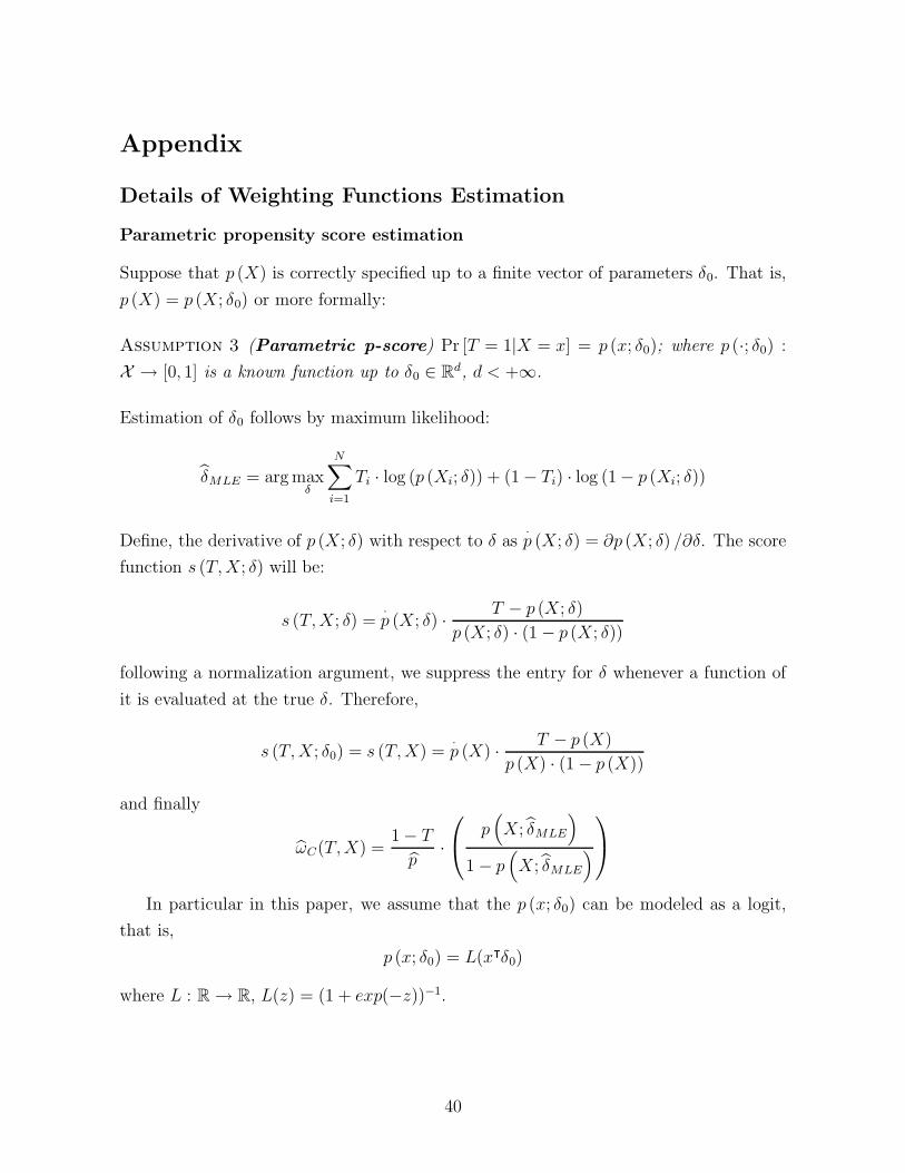
Appendix

Details of Weighting Functions Estimation

Parametric propensity score estimation

Suppose that p (X) is correctly specified up to a finite vector of parameters δ0. That is,

p (X) = p (X; δ0) or more formally:

Assumption 3 (Parametric p-score) Pr [T = 1|X = x] = p (x; δ0); where p (·; δ0) :

X → [0, 1] is a known function up to δ0 ∈ Rd, d < +∞.

Estimation of δ0 follows by maximum likelihood:

δMLE = arg maxδ

N∑

i=1

Ti · log (p (Xi; δ)) + (1 − Ti) · log (1 − p (Xi; δ))

Define, the derivative of p (X; δ) with respect to δ as·p (X; δ) = ∂p (X; δ) /∂δ. The score

function s (T,X; δ) will be:

s (T,X; δ) =·p (X; δ) · T − p (X; δ)

p (X; δ) · (1 − p (X; δ))

following a normalization argument, we suppress the entry for δ whenever a function of

it is evaluated at the true δ. Therefore,

s (T,X; δ0) = s (T,X) =·p (X) · T − p (X)

p (X) · (1 − p (X))

and finally

ωC(T,X) =1 − T

p·

p(X; δMLE

)

1 − p(X; δMLE

)

In particular in this paper, we assume that the p (x; δ0) can be modeled as a logit,

that is,

p (x; δ0) = L(xᵀδ0)

where L : R → R, L(z) = (1 + exp(−z))−1.

40

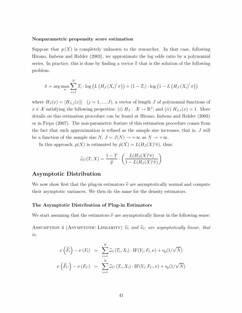
Nonparametric propensity score estimation

Suppose that p (X) is completely unknown to the researcher. In that case, following

Hirano, Imbens and Ridder (2003), we approximate the log odds ratio by a polynomial

series. In practice, this is done by finding a vector π that is the solution of the following

problem:

π = arg maxπ

N∑

i=1

Ti · log(L(HJ (Xi)

′ π))

+ (1 − Ti) · log(1 − L

(HJ (Xi)

′ π))

where HJ (x) = [HJ, j(x)] (j = 1, ..., J), a vector of length J of polynomial functions of

x ∈ X satisfying the following properties: (i) HJ : X → RJ ; and (ii) HJ, 1(x) = 1. More

details on this estimation procedure can be found at Hirano, Imbens and Ridder (2003)

or in Firpo (2007). The non-parametric feature of this estimation procedure comes from

the fact that such approximation is refined as the sample size increases, that is, J will

be a function of the sample size N, J = J(N) → +∞ as N → +∞.

In this approach, p(X) is estimated by p(X) = L(HJ (X)′π), thus:

ωC(T,X) =1 − T

p·(

L(HJ (X)′π)

1 − L(HJ (X)′π)

)

Asymptotic Distribution

We now show first that the plug-in estimators ν are asymptotically normal and compute

their asymptotic variances. We then do the same for the density estimators.

The Asymptotic Distribution of Plug-in Estimators

We start assuming that the estimators ν are asymptotically linear in the following sense:

Assumption 4 (Asymptotic Linearity) νt and νC are asymptotically linear, that

is,

ν(Ft

)− ν (Ft) =

N∑

i=1

ωt (Ti,Xi) · IF(Yi;Ft, ν) + op(1/√N)

ν(FC

)− ν (FC) =

N∑

i=1

ωC (Ti,Xi) · IF(Yi;FC, ν) + op(1/√N)

41

Assumption 4 establishes that estimators are either exactly linear, as those that are

based on sample moments, or they can be linearized and the remainder term will approach

zero as the sample size increases.

An additional technical assumption is that the influence function are square integrable

and its conditional expectation given X differentiable. To simplify notation, let us write

IF(Yt;F, ν) = ψνt (Y ).

Assumption 5 [Influence Function] For all weighting functions ω considered,

(i) E[(ψν

t (Y ;Ft))2] <∞, E

[(ψν

C (Y ;FC))2] <∞ and

(ii) E [ψνt (Y ;Ft) |X = x] E [ψν

C (Y ;FC) |X = x] and are continuously differentiable for

all x in X .

Under ignorability both types of estimators (parametric and non-parametric first step)

for ν1, ν0, and νC proposed before will remain asymptotically linear. The theorem below

consider both the parametric and non-parametric two cases.

Theorem 3 [Asymptotic Normality of the ν Estimators]:

Under assumptions 1, 2, 4 and 5:

(i-ii)√N · (νt − νt) = 1√

N

∑Ni=1 ωt(Ti) · ψν (Yi;Ft) + op(1)

D→ N (0, Vt), t = 0, 1

(iii) (a) if in addition, Assumption 3 holds, then:

√N · (νC − νC) =

1√N

N∑

i=1

ωC(Ti,Xi) · ψν (Yi;FC)

+ (ω1(Ti) − ωC(Ti,Xi)) ··p (Xi)

′

p (Xi)· (E [s (T,X) · s (T,X)ᵀ])

−1

· E

[ ·p (X)

1 − p (X)· E [ψν

C (Y ;FC) | X,T = 0]

]+ op(1)

D→ N (0, VC,P )

(iii) (b) otherwise, if in addition we assume [non-parametric], then:

√N · (νC − νC) =

1√N

N∑

i=1

ωC(Ti,Xi) · ψν (Yi;FC)

+ (ω1(Ti) − ωC(Ti,Xi)) · E [ψνC (Y ;FC) | Xi, T = 0] + op(1)

D→ N (0, VC,NP )

where

Vt = E[(ωt(T ) · ψν

t (Y ;Ft))2] , t = 0, 1

42

VC,P = E

[(ωC(T,X) · ψν (Y ;FC)

+ (ω1(T ) − ωC(T,X)) ··p (X)′

p (X)· (E [s (T,X) · s (T,X)ᵀ])

−1

· E

[ ·p (X)

1 − p (X)· E [ψν

C (Y ;FC) | X,T = 0]

])2]

VC,NP = E

[(ωC(T,X) · ψν (Y,X;FC)

+ (ω1(T )− ωC(T,X)) · E [ψνC (Y,X;FC) | X,T = 0]

)2]

Proofs

Proof of Theorem 1: A proof can be found in Firpo (2007b).

�

Proof of Theorem 2: Part (i) is straightforward and follows from identification of the

functionals ν1, ν0 and νC, a direct consequence of identification of F1, F0 and FC. Part

(ii) follows from the fact that

F1 (y) = E [E [1I{g1 (X, ε) ≤ y} | T = 1,X]]

=E[E [1I{g0 (X, ε) ≤ y} | T = 1,X]

+E [1I{g1 (X, ε) ≤ y} − 1I{g0 (X, ε) ≤ y} | T = 1,X] ]

= FC (y) + F1−0 (y)

where

F1−0 (y) = E [E [1I{g1 (X, ε) ≤ y} − 1I{g0 (X, ε) ≤ y} | T = 1,X]]

thus, if g1 (·, ·) = g0 (·, ·), then for all y, F1−0 (y) = 0 and

ν1 = ν (F1) = ν (FC + F1−0) = ν (FC) = νC .

43

Part (iii) follows by a similar argument:

F0 (y) =

∫Pr [Y0 ≤ y | T = 0,X = x] · dFX |T (x|0) · dx

=

∫Pr [Y0 ≤ y | T = 0,X = x] · dFX |T (x|1) · dx

+

∫Pr [Y0 ≤ y | T = 0,X = x] ·

(dFX |T (x|0) − dFX |T (x|1)

)· dx

= FC (y) + F∆ (y)

where

F∆ (y) =

∫Pr [Y0 ≤ y | T = 0,X = x] · d

(FX |T (x|0) − FX |T (x|1)

)· dx

thus if FX |T (·|1) = FX |T (·|0), then for all x, FX |T (x|1) − FX |T (x|0) = 0 and therefore,

for all y, F∆ (y) = 0 and

ν0 = ν (F0) = ν (FC + F∆) = ν (FC) = νC .

�

Proof of Theorem 3 A proof of parts (i), (ii) and (iii) (b) can be found in Firpo

(2007b). A proof of part (iii) (a) can be found in Chen, Hong and Tarozzi (2006).

�

44

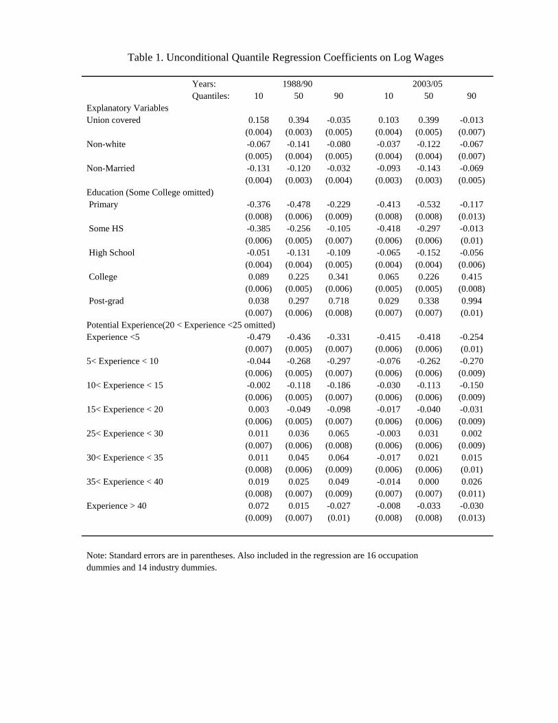
Table 1. Unconditional Quantile Regression Coefficients on Log Wages Years: 1988/90 2003/05 Quantiles: 10 50 90 10 50 90 Explanatory Variables Union covered 0.158 0.394 -0.035 0.103 0.399 -0.013 (0.004) (0.003) (0.005) (0.004) (0.005) (0.007) Non-white -0.067 -0.141 -0.080 -0.037 -0.122 -0.067 (0.005) (0.004) (0.005) (0.004) (0.004) (0.007) Non-Married -0.131 -0.120 -0.032 -0.093 -0.143 -0.069 (0.004) (0.003) (0.004) (0.003) (0.003) (0.005) Education (Some College omitted) Primary -0.376 -0.478 -0.229 -0.413 -0.532 -0.117 (0.008) (0.006) (0.009) (0.008) (0.008) (0.013) Some HS -0.385 -0.256 -0.105 -0.418 -0.297 -0.013 (0.006) (0.005) (0.007) (0.006) (0.006) (0.01) High School -0.051 -0.131 -0.109 -0.065 -0.152 -0.056 (0.004) (0.004) (0.005) (0.004) (0.004) (0.006) College 0.089 0.225 0.341 0.065 0.226 0.415 (0.006) (0.005) (0.006) (0.005) (0.005) (0.008) Post-grad 0.038 0.297 0.718 0.029 0.338 0.994 (0.007) (0.006) (0.008) (0.007) (0.007) (0.01) Potential Experience(20 < Experience <25 omitted) Experience <5 -0.479 -0.436 -0.331 -0.415 -0.418 -0.254 (0.007) (0.005) (0.007) (0.006) (0.006) (0.01) 5< Experience < 10 -0.044 -0.268 -0.297 -0.076 -0.262 -0.270 (0.006) (0.005) (0.007) (0.006) (0.006) (0.009) 10< Experience < 15 -0.002 -0.118 -0.186 -0.030 -0.113 -0.150 (0.006) (0.005) (0.007) (0.006) (0.006) (0.009) 15< Experience < 20 0.003 -0.049 -0.098 -0.017 -0.040 -0.031 (0.006) (0.005) (0.007) (0.006) (0.006) (0.009) 25< Experience < 30 0.011 0.036 0.065 -0.003 0.031 0.002 (0.007) (0.006) (0.008) (0.006) (0.006) (0.009) 30< Experience < 35 0.011 0.045 0.064 -0.017 0.021 0.015 (0.008) (0.006) (0.009) (0.006) (0.006) (0.01) 35< Experience < 40 0.019 0.025 0.049 -0.014 0.000 0.026 (0.008) (0.007) (0.009) (0.007) (0.007) (0.011) Experience > 40 0.072 0.015 -0.027 -0.008 -0.033 -0.030 (0.009) (0.007) (0.01) (0.008) (0.008) (0.013) Note: Standard errors are in parentheses. Also included in the regression are 16 occupation dummies and 14 industry dummies.

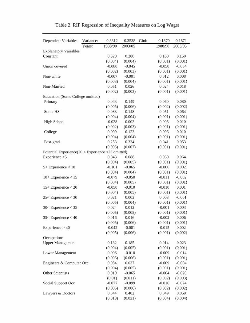
Table 2. RIF Regression of Inequality Measures on Log Wages

Dependent Variables Variance: 0.3312 0.3538 Gini: 0.1870 0.1871

Years: 1988/90 2003/05 1988/90 2003/05Explanatory VariablesConstant 0.320 0.280 0.160 0.150

(0.004) (0.004) (0.001) (0.001)Union covered -0.080 -0.045 -0.050 -0.034

(0.002) (0.003) (0.001) (0.001)Non-white -0.007 -0.001 0.012 0.008

(0.003) (0.004) (0.001) (0.001)Non-Married 0.051 0.026 0.024 0.018

(0.002) (0.003) (0.001) (0.001)Education (Some College omitted) Primary 0.043 0.149 0.060 0.080

(0.005) (0.006) (0.002) (0.002) Some HS 0.083 0.148 0.051 0.064

(0.004) (0.004) (0.001) (0.001) High School -0.028 0.002 0.005 0.010

(0.002) (0.003) (0.001) (0.001) College 0.099 0.123 0.006 0.010

(0.004) (0.004) (0.001) (0.001) Post-grad 0.253 0.334 0.041 0.053

(0.005) (0.007) (0.001) (0.001)Potential Experience(20 < Experience <25 omitted)Experience <5 0.043 0.088 0.060 0.064

(0.004) (0.005) (0.001) (0.001)5< Experience < 10 -0.101 -0.065 -0.006 0.002

(0.004) (0.004) (0.001) (0.001)10< Experience < 15 -0.079 -0.050 -0.011 -0.002

(0.004) (0.005) (0.001) (0.001)15< Experience < 20 -0.050 -0.010 -0.010 0.001

(0.004) (0.005) (0.001) (0.001)25< Experience < 30 0.021 0.002 0.003 -0.001

(0.005) (0.004) (0.001) (0.001)30< Experience < 35 0.024 0.012 -0.001 0.003

(0.005) (0.005) (0.001) (0.001)35< Experience < 40 0.016 0.016 -0.002 0.006

(0.005) (0.006) (0.001) (0.001)Experience > 40 -0.042 -0.001 -0.015 0.002

(0.005) (0.006) (0.001) (0.002)Occupations Upper Management 0.132 0.185 0.014 0.023

(0.004) (0.005) (0.001) (0.001)Lower Management 0.006 -0.010 -0.009 -0.014

(0.006) (0.006) (0.001) (0.001)Engineers & Computer Occ. 0.034 0.037 -0.009 -0.004

(0.004) (0.005) (0.001) (0.001)Other Scientists 0.010 -0.065 -0.004 -0.020

(0.01) (0.011) (0.002) (0.003)Social Support Occ -0.077 -0.099 -0.016 -0.024

(0.005) (0.006) (0.002) (0.002)Lawyers & Doctors 0.344 0.402 0.049 0.069

(0.018) (0.021) (0.004) (0.004)

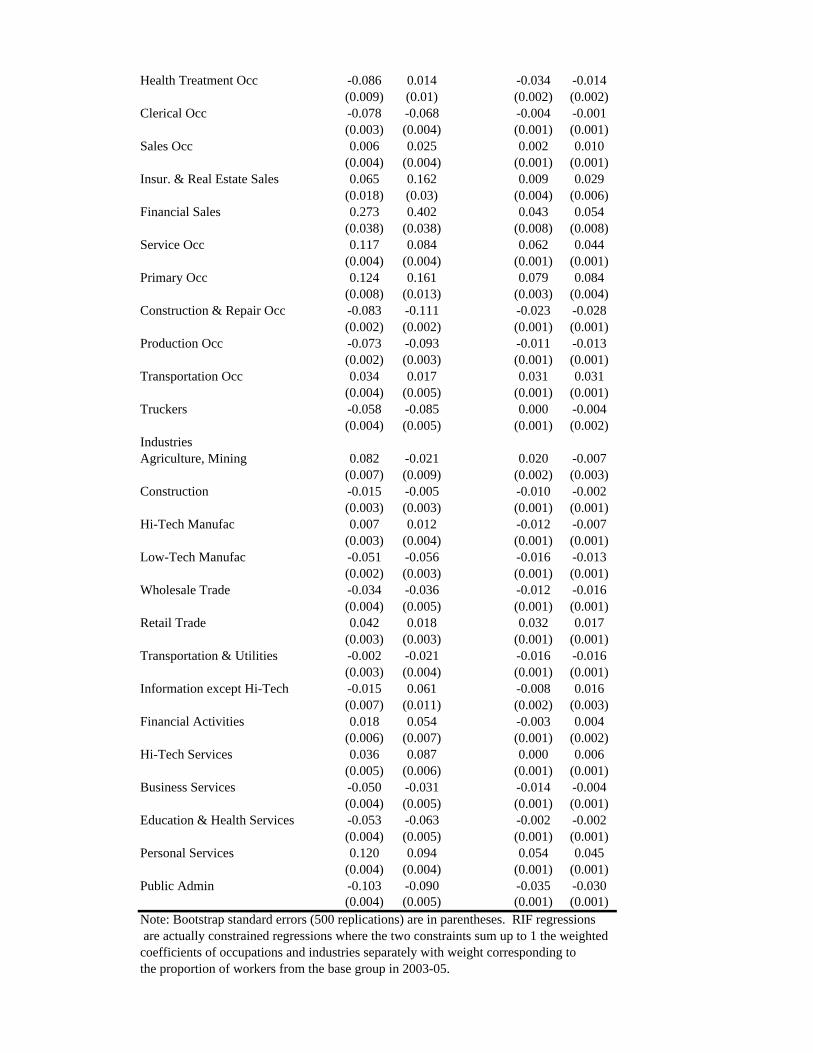
Health Treatment Occ -0.086 0.014 -0.034 -0.014(0.009) (0.01) (0.002) (0.002)

Clerical Occ -0.078 -0.068 -0.004 -0.001(0.003) (0.004) (0.001) (0.001)

Sales Occ 0.006 0.025 0.002 0.010(0.004) (0.004) (0.001) (0.001)

Insur. & Real Estate Sales 0.065 0.162 0.009 0.029(0.018) (0.03) (0.004) (0.006)

Financial Sales 0.273 0.402 0.043 0.054(0.038) (0.038) (0.008) (0.008)

Service Occ 0.117 0.084 0.062 0.044(0.004) (0.004) (0.001) (0.001)

Primary Occ 0.124 0.161 0.079 0.084(0.008) (0.013) (0.003) (0.004)

Construction & Repair Occ -0.083 -0.111 -0.023 -0.028(0.002) (0.002) (0.001) (0.001)

Production Occ -0.073 -0.093 -0.011 -0.013(0.002) (0.003) (0.001) (0.001)

Transportation Occ 0.034 0.017 0.031 0.031(0.004) (0.005) (0.001) (0.001)

Truckers -0.058 -0.085 0.000 -0.004(0.004) (0.005) (0.001) (0.002)

IndustriesAgriculture, Mining 0.082 -0.021 0.020 -0.007

(0.007) (0.009) (0.002) (0.003)Construction -0.015 -0.005 -0.010 -0.002

(0.003) (0.003) (0.001) (0.001)Hi-Tech Manufac 0.007 0.012 -0.012 -0.007

(0.003) (0.004) (0.001) (0.001)Low-Tech Manufac -0.051 -0.056 -0.016 -0.013

(0.002) (0.003) (0.001) (0.001)Wholesale Trade -0.034 -0.036 -0.012 -0.016

(0.004) (0.005) (0.001) (0.001)Retail Trade 0.042 0.018 0.032 0.017

(0.003) (0.003) (0.001) (0.001)Transportation & Utilities -0.002 -0.021 -0.016 -0.016

(0.003) (0.004) (0.001) (0.001)Information except Hi-Tech -0.015 0.061 -0.008 0.016

(0.007) (0.011) (0.002) (0.003)Financial Activities 0.018 0.054 -0.003 0.004

(0.006) (0.007) (0.001) (0.002)Hi-Tech Services 0.036 0.087 0.000 0.006

(0.005) (0.006) (0.001) (0.001)Business Services -0.050 -0.031 -0.014 -0.004

(0.004) (0.005) (0.001) (0.001)Education & Health Services -0.053 -0.063 -0.002 -0.002

(0.004) (0.005) (0.001) (0.001)Personal Services 0.120 0.094 0.054 0.045

(0.004) (0.004) (0.001) (0.001)Public Admin -0.103 -0.090 -0.035 -0.030

(0.004) (0.005) (0.001) (0.001)Note: Bootstrap standard errors (500 replications) are in parentheses. RIF regressions are actually constrained regressions where the two constraints sum up to 1 the weighted coefficients of occupations and industries separately with weight corresponding to the proportion of workers from the base group in 2003-05.

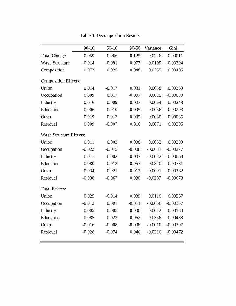
Table 3. Decomposition Results

90-10 50-10 90-50 Variance GiniTotal Change 0.059 -0.066 0.125 0.0226 0.00011Wage Structure -0.014 -0.091 0.077 -0.0109 -0.00394Composition 0.073 0.025 0.048 0.0335 0.00405

Composition Effects:Union 0.014 -0.017 0.031 0.0058 0.00359Occupation 0.009 0.017 -0.007 0.0025 -0.00080Industry 0.016 0.009 0.007 0.0064 0.00248Education 0.006 0.010 -0.005 0.0036 -0.00293Other 0.019 0.013 0.005 0.0080 -0.00035Residual 0.009 -0.007 0.016 0.0071 0.00206

Wage Structure Effects:Union 0.011 0.003 0.008 0.0052 0.00209Occupation -0.022 -0.015 -0.006 -0.0081 -0.00277Industry -0.011 -0.003 -0.007 -0.0022 -0.00068Education 0.080 0.013 0.067 0.0320 0.00781Other -0.034 -0.021 -0.013 -0.0091 -0.00362Residual -0.038 -0.067 0.030 -0.0287 -0.00678

Total Effects: Union 0.025 -0.014 0.039 0.0110 0.00567Occupation -0.013 0.001 -0.014 -0.0056 -0.00357Industry 0.005 0.005 0.000 0.0042 0.00180Education 0.085 0.023 0.062 0.0356 0.00488Other -0.016 -0.008 -0.008 -0.0010 -0.00397Residual -0.028 -0.074 0.046 -0.0216 -0.00472

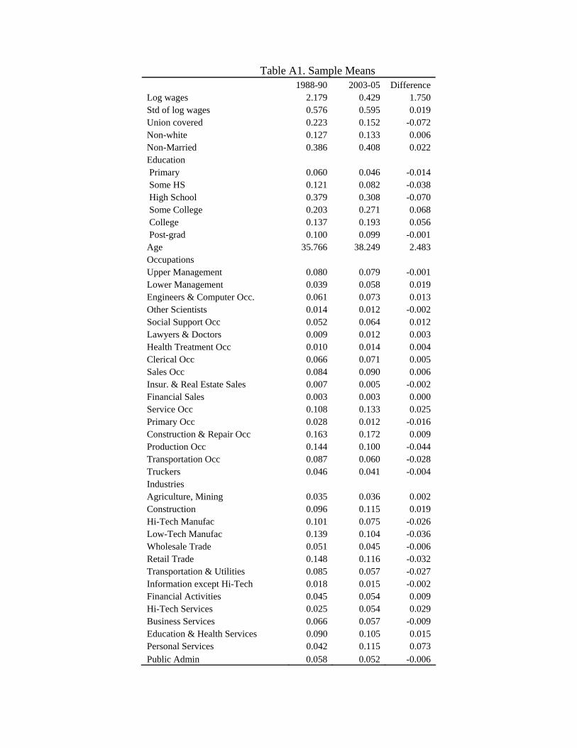
Table A1. Sample Means 1988-90 2003-05 Difference Log wages 2.179 0.429 1.750 Std of log wages 0.576 0.595 0.019 Union covered 0.223 0.152 -0.072 Non-white 0.127 0.133 0.006 Non-Married 0.386 0.408 0.022 Education Primary 0.060 0.046 -0.014 Some HS 0.121 0.082 -0.038 High School 0.379 0.308 -0.070 Some College 0.203 0.271 0.068 College 0.137 0.193 0.056 Post-grad 0.100 0.099 -0.001 Age 35.766 38.249 2.483 Occupations Upper Management 0.080 0.079 -0.001 Lower Management 0.039 0.058 0.019 Engineers & Computer Occ. 0.061 0.073 0.013 Other Scientists 0.014 0.012 -0.002 Social Support Occ 0.052 0.064 0.012 Lawyers & Doctors 0.009 0.012 0.003 Health Treatment Occ 0.010 0.014 0.004 Clerical Occ 0.066 0.071 0.005 Sales Occ 0.084 0.090 0.006 Insur. & Real Estate Sales 0.007 0.005 -0.002 Financial Sales 0.003 0.003 0.000 Service Occ 0.108 0.133 0.025 Primary Occ 0.028 0.012 -0.016 Construction & Repair Occ 0.163 0.172 0.009 Production Occ 0.144 0.100 -0.044 Transportation Occ 0.087 0.060 -0.028 Truckers 0.046 0.041 -0.004 Industries Agriculture, Mining 0.035 0.036 0.002 Construction 0.096 0.115 0.019 Hi-Tech Manufac 0.101 0.075 -0.026 Low-Tech Manufac 0.139 0.104 -0.036 Wholesale Trade 0.051 0.045 -0.006 Retail Trade 0.148 0.116 -0.032 Transportation & Utilities 0.085 0.057 -0.027 Information except Hi-Tech 0.018 0.015 -0.002 Financial Activities 0.045 0.054 0.009 Hi-Tech Services 0.025 0.054 0.029 Business Services 0.066 0.057 -0.009 Education & Health Services 0.090 0.105 0.015 Personal Services 0.042 0.115 0.073 Public Admin 0.058 0.052 -0.006

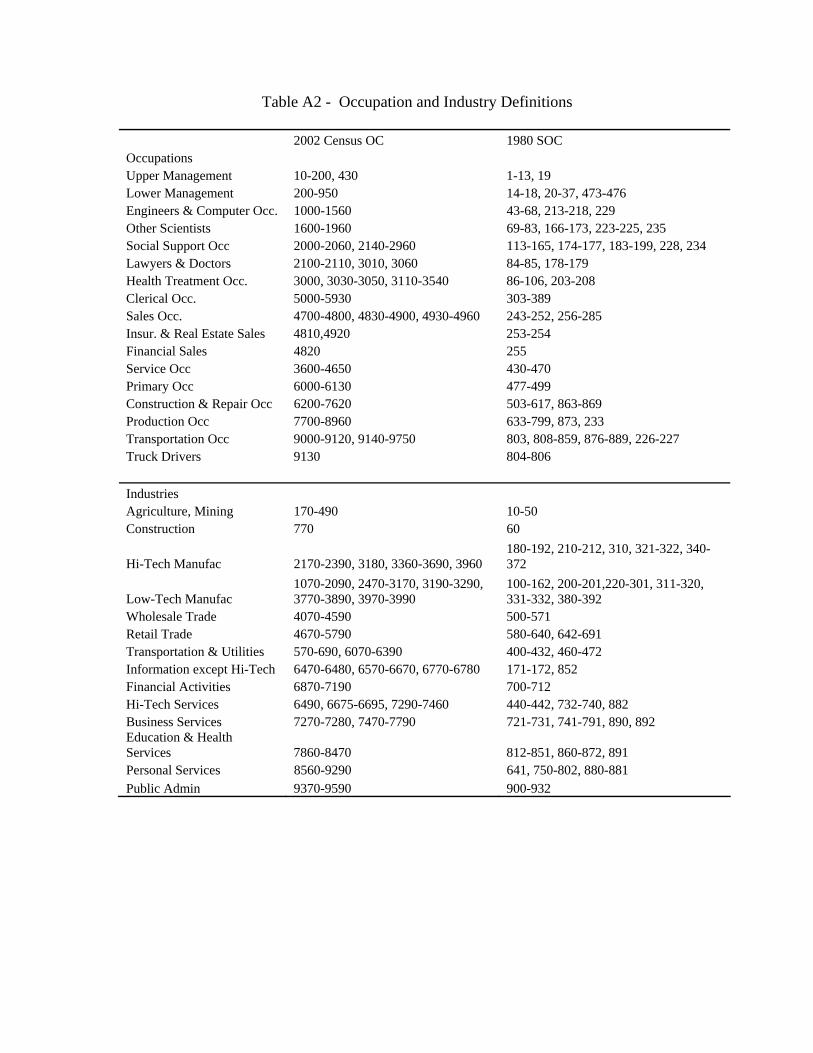
Table A2 - Occupation and Industry Definitions 2002 Census OC 1980 SOC Occupations Upper Management 10-200, 430 1-13, 19 Lower Management 200-950 14-18, 20-37, 473-476 Engineers & Computer Occ. 1000-1560 43-68, 213-218, 229 Other Scientists 1600-1960 69-83, 166-173, 223-225, 235 Social Support Occ 2000-2060, 2140-2960 113-165, 174-177, 183-199, 228, 234 Lawyers & Doctors 2100-2110, 3010, 3060 84-85, 178-179 Health Treatment Occ. 3000, 3030-3050, 3110-3540 86-106, 203-208 Clerical Occ. 5000-5930 303-389 Sales Occ. 4700-4800, 4830-4900, 4930-4960 243-252, 256-285 Insur. & Real Estate Sales 4810,4920 253-254 Financial Sales 4820 255 Service Occ 3600-4650 430-470 Primary Occ 6000-6130 477-499 Construction & Repair Occ 6200-7620 503-617, 863-869 Production Occ 7700-8960 633-799, 873, 233 Transportation Occ 9000-9120, 9140-9750 803, 808-859, 876-889, 226-227 Truck Drivers 9130 804-806 Industries Agriculture, Mining 170-490 10-50 Construction 770 60

Hi-Tech Manufac 2170-2390, 3180, 3360-3690, 3960 180-192, 210-212, 310, 321-322, 340-372

Low-Tech Manufac 1070-2090, 2470-3170, 3190-3290, 3770-3890, 3970-3990

100-162, 200-201,220-301, 311-320, 331-332, 380-392

Wholesale Trade 4070-4590 500-571 Retail Trade 4670-5790 580-640, 642-691 Transportation & Utilities 570-690, 6070-6390 400-432, 460-472 Information except Hi-Tech 6470-6480, 6570-6670, 6770-6780 171-172, 852 Financial Activities 6870-7190 700-712 Hi-Tech Services 6490, 6675-6695, 7290-7460 440-442, 732-740, 882 Business Services 7270-7280, 7470-7790 721-731, 741-791, 890, 892 Education & Health Services 7860-8470 812-851, 860-872, 891 Personal Services 8560-9290 641, 750-802, 880-881 Public Admin 9370-9590 900-932

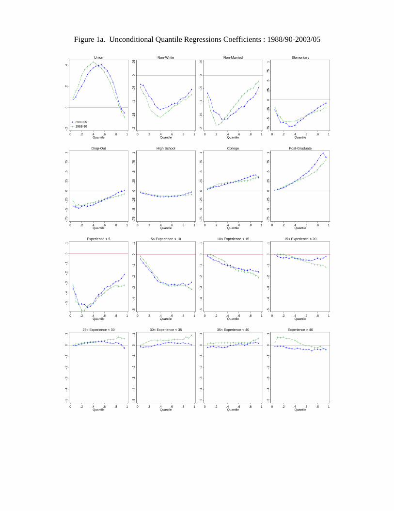
Figure 1a. Unconditional Quantile Regressions Coefficients : 1988/90-2003/05

-.20

.2.4

0 .2 .4 .6 .8 1Quantile

2003-051988-90

Union

-.2-.1

5-.1

-.05

0.0

5

0 .2 .4 .6 .8 1Quantile

Non-White

-.2-.1

5-.1

-.05

0.0

5

0 .2 .4 .6 .8 1Quantile

Non-Married

-.75

-.5-.2

50

.25

.5.7

51

0 .2 .4 .6 .8 1Quantile

Elementary

-.75

-.5-.2

50

.25

.5.7

51

0 .2 .4 .6 .8 1Quantile

Drop-Out

-.75

-.5-.2

50

.25

.5.7

51

0 .2 .4 .6 .8 1Quantile

High School

-.75

-.5-.2

50

.25

.5.7

51

0 .2 .4 .6 .8 1Quantile

College

-.75

-.5-.2

50

.25

.5.7

51

0 .2 .4 .6 .8 1Quantile

Post-Graduate

-.5-.4

-.3-.2

-.10

.1

0 .2 .4 .6 .8 1Quantile

Experience < 5

-.5-.4

-.3-.2

-.10

.1

0 .2 .4 .6 .8 1Quantile

5< Experience < 10

-.5-.4

-.3-.2

-.10

.1

0 .2 .4 .6 .8 1Quantile

10< Experience < 15

-.5-.4

-.3-.2

-.10

.1

0 .2 .4 .6 .8 1Quantile

15< Experience < 20

-.5-.4

-.3-.2

-.10

.1

0 .2 .4 .6 .8 1Quantile

25< Experience < 30

-.5-.4

-.3-.2

-.10

.1

0 .2 .4 .6 .8 1Quantile

30< Experience < 35

-.5-.4

-.3-.2

-.10

.1

0 .2 .4 .6 .8 1Quantile

35< Experience < 40

-.5-.4

-.3-.2

-.10

.1

0 .2 .4 .6 .8 1Quantile

Experience > 40

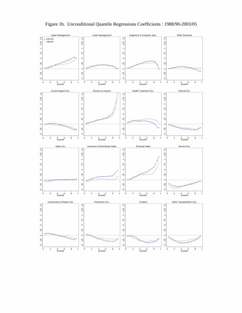
Figure 1b. Unconditional Quantile Regressions Coefficients : 1988/90-2003/05

-.5-.2

50

.25

.5.7

51

1.25

1.5

0 .2 .4 .6 .8 1Quantile

2003-051988-90

Upper Management

-.5-.2

50

.25

.5.7

51

1.25

1.5

0 .2 .4 .6 .8 1

Quantile

Lower Management

-.5-.2

50

.25

.5.7

51

1.25

1.5

0 .2 .4 .6 .8 1Quantile

Engineers & Computer spec.

-.5-.2

50

.25

.5.7

51

1.25

1.5

0 .2 .4 .6 .8 1Quantile

Other Scientists

-.5-.2

50

.25

.5.7

51

1.25

1.5

0 .2 .4 .6 .8 1Quantile

Social Support Occ.

-.5-.2

50

.25

.5.7

51

1.25

1.5

0 .2 .4 .6 .8 1Quantile

Doctors & Lawyers

-.5-.2

50

.25

.5.7

51

1.25

1.5

0 .2 .4 .6 .8 1Quantile

Health Treatment Occ.

-.5-.2

50

.25

.5.7

51

1.25

1.5

0 .2 .4 .6 .8 1Quantile

Clerical Occ.

-.5-.2

50

.25

.5.7

51

1.25

1.5

0 .2 .4 .6 .8 1Quantile

Sales Occ.

-.5-.2

50

.25

.5.7

51

1.25

1.5

0 .2 .4 .6 .8 1Quantile

Insurance & Real Estate Sales

-.5-.2

50

.25

.5.7

51

1.25

1.5

0 .2 .4 .6 .8 1Quantile

Financial Sales

-.5-.2

50

.25

.5.7

51

1.25

1.5

0 .2 .4 .6 .8 1Quantile

Service Occ.

-.5-.2

50

.25

.5.7

51

1.25

1.5

0 .2 .4 .6 .8 1Quantile

Construction & Repair Occ.

-.5-.2

50

.25

.5.7

51

1.25

1.5

0 .2 .4 .6 .8 1Quantile

Production Occ.

-.5-.2

50

.25

.5.7

51

1.25

1.5

0 .2 .4 .6 .8 1Quantile

Truckers

-.5-.2

50

.25

.5.7

51

1.25

1.5

0 .2 .4 .6 .8 1Quantile

Other Transportation Occ.

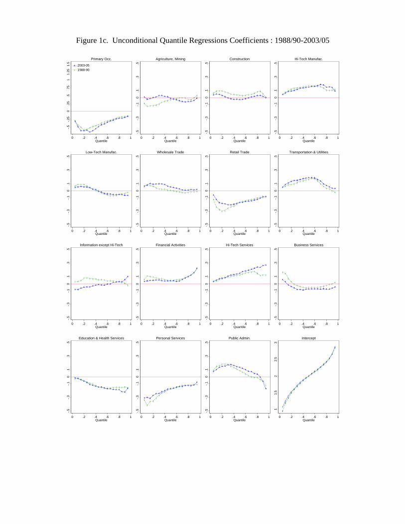
Figure 1c. Unconditional Quantile Regressions Coefficients : 1988/90-2003/05

-.5-.2

50

.25

.5.7

51

1.25

1.5

0 .2 .4 .6 .8 1Quantile

2003-051988-90

Primary Occ.

-.5-.3

-.10

.1.3

.5

0 .2 .4 .6 .8 1Quantile

Agriculture, Mining

-.5-.3

-.10

.1.3

.5

0 .2 .4 .6 .8 1Quantile

Construction

-.5-.3

-.10

.1.3

.5

0 .2 .4 .6 .8 1Quantile

Hi-Tech Manufac.

-.5-.3

-.10

.1.3

.5

0 .2 .4 .6 .8 1Quantile

Low-Tech Manufac.

-.5-.3

-.10

.1.3

.5

0 .2 .4 .6 .8 1Quantile

Wholesale Trade

-.5-.3

-.10

.1.3

.5

0 .2 .4 .6 .8 1Quantile

Retail Trade

-.5-.3

-.10

.1.3

.5

0 .2 .4 .6 .8 1Quantile

Transportation & Utilities

-.5-.3

-.10

.1.3

.5

0 .2 .4 .6 .8 1Quantile

Information except Hi-Tech

-.5-.3

-.10

.1.3

.5

0 .2 .4 .6 .8 1Quantile

Financial Activities

-.5-.3

-.10

.1.3

.5

0 .2 .4 .6 .8 1Quantile

Hi-Tech Services

-.5-.3

-.10

.1.3

.5

0 .2 .4 .6 .8 1Quantile

Business Services

-.5-.3

-.10

.1.3

.5

0 .2 .4 .6 .8 1Quantile

Education & Health Services

-.5-.3

-.10

.1.3

.5

0 .2 .4 .6 .8 1Quantile

Personal Services

-.5-.3

-.10

.1.3

.5

0 .2 .4 .6 .8 1Quantile

Public Admin.

11.

52

2.5

3

0 .2 .4 .6 .8 1Quantile

Intercept

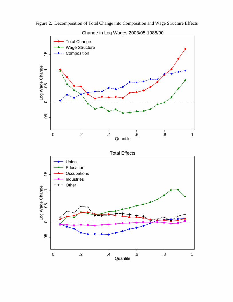
Figure 2. Decomposition of Total Change into Composition and Wage Structure Effects

-.05

0.0

5.1

.15

Log

Wag

e C

hang

e

0 .2 .4 .6 .8 1Quantile

Total ChangeWage StructureComposition

Change in Log Wages 2003/05-1988/90

-.05

0.0

5.1

.15

Log

Wag

e C

hang

e

0 .2 .4 .6 .8 1Quantile

UnionEducationOccupationsIndustriesOther

Total Effects

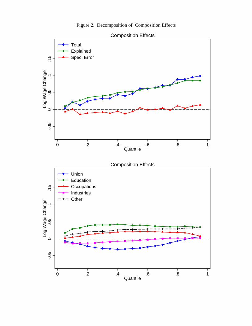
Figure 2. Decomposition of Composition Effects

-.05

0.0

5.1

.15

Log

Wag

e C

hang

e

0 .2 .4 .6 .8 1Quantile

TotalExplainedSpec. Error

Composition Effects

-.05

0.0

5.1

.15

Log

Wag

e C

hang

e

0 .2 .4 .6 .8 1Quantile

UnionEducationOccupationsIndustriesOther

Composition Effects

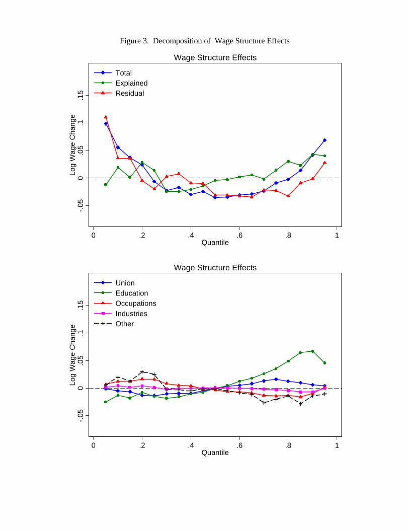
Figure 3. Decomposition of Wage Structure Effects

-.05

0.0

5.1

.15

Log

Wag

e C

hang

e

0 .2 .4 .6 .8 1Quantile

TotalExplainedResidual

Wage Structure Effects

-.05

0.0

5.1

.15

Log

Wag

e C

hang

e

0 .2 .4 .6 .8 1Quantile

UnionEducationOccupationsIndustriesOther

Wage Structure Effects

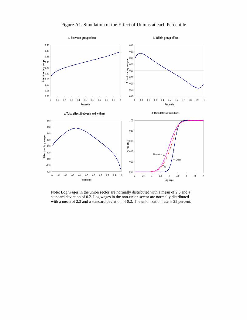
Figure A1. Simulation of the Effect of Unions at each Percentile

a. Between-group effect

0.00

0.05

0.10

0.15

0.20

0.25

0.30

0.35

0.40

0.45

0 0.1 0.2 0.3 0.4 0.5 0.6 0.7 0.8 0.9 1

Percentile

Effe

ct o

n lo

g w

age

b. Within-group effect

-0.40

-0.30

-0.20

-0.10

0.00

0.10

0.20

0.30

0.40

0 0.1 0.2 0.3 0.4 0.5 0.6 0.7 0.8 0.9 1

Percentile

Effe

ct o

n lo

g w

ages

c. Total effect (between and within)

-0.20

-0.10

0.00

0.10

0.20

0.30

0.40

0.50

0.60

0 0.1 0.2 0.3 0.4 0.5 0.6 0.7 0.8 0.9 1

Percentile

Effe

ct o

n lo

g w

ages

d. Cumulative distributions

0.00

0.20

0.40

0.60

0.80

1.00

0 0.5 1 1.5 2 2.5 3 3.5 4

Log wage

Perc

entil

e

Union

Non-union

All

Note: Log wages in the union sector are normally distributed with a mean of 2.3 and a standard deviation of 0.2. Log wages in the non-union sector are normally distributed with a mean of 2.3 and a standard deviation of 0.2. The unionization rate is 25 percent.

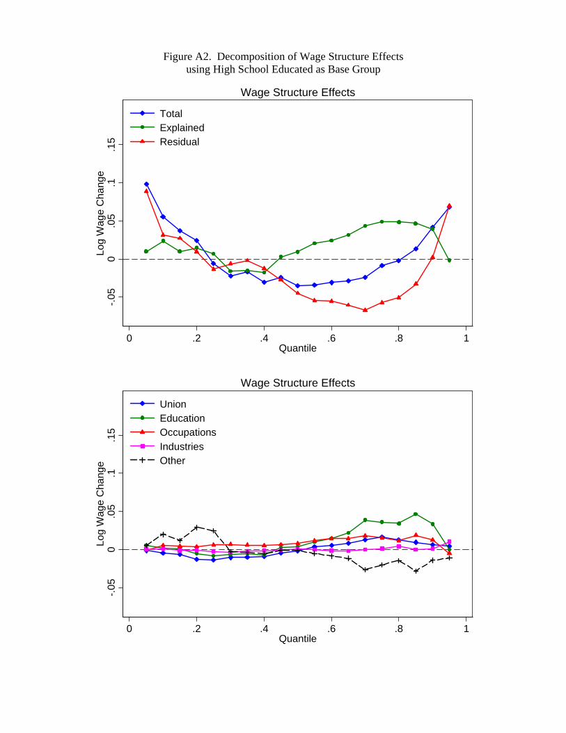
Figure A2. Decomposition of Wage Structure Effects using High School Educated as Base Group

-.05

0.0

5.1

.15

Log

Wag

e C

hang

e

0 .2 .4 .6 .8 1Quantile

TotalExplainedResidual

Wage Structure Effects-.0

50

.05

.1.1

5Lo

g W

age

Cha

nge

0 .2 .4 .6 .8 1Quantile

UnionEducationOccupationsIndustriesOther

Wage Structure Effects

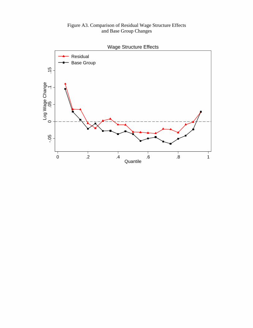
Figure A3. Comparison of Residual Wage Structure Effects and Base Group Changes

-.05

0.0

5.1

.15

Log

Wag

e C

hang

e

0 .2 .4 .6 .8 1Quantile

ResidualBase Group

Wage Structure Effects