Decomposing Wage Distributions: Estimation and Inference

Sergio FirpoUBC and PUC-Rio

Nicole FortinUBC

Thomas LemieuxUBC

Preliminary and incomplete, July 2005

Abstract

The paper generalizes the standard Oaxaca-Blinder decomposition (a popular tool ofpolicy analysis) in two important ways: 1) by applying this type of decomposition to anydistributional features and not only the mean, and 2) by allowing for a much more �exiblewage setting model. In this paper, we focus on wage decompositions but the method alsoapplies to any other outcome variable. We estimate directly the elements of the decompo-sition instead of �rst estimating a structural wage-setting model, and indirectly computingthe elements of the decomposition using structural parameters. We propose a two-stepmethod to do the decomposition. In Step 1, overall wage gap is divided into a wage struc-ture e¤ect and a composition e¤ect using a (propensity score) reweighting method. In Step2, these two terms are further divided into the contribution of each individual explanatoryvariable using a (novel) in�uence function projection technique. Finally, we illustrate howthe method works in practice using three empirical examples.

1

1 Introduction

Oaxaca-Blinder decompositions are a popular tool of policy analysis that have been appliedto a wide range of empirical problems. Two key advantages of the approach is that it issimple to implement and easy to interpret. However, simplicity and convenience come at somecosts. First, the procedure can only be used to decompose the mean of outcome variables. Forexample, the initial application of the decomposition was to the case of gender wage gap. More,recently, however, there has been growing interest for how the gender gap varies at di¤erentpoints of the wage distribution (glass ceiling, etc.). More importantly, the large increase inwage an earnings inequality in the United States over the last 25 years have raised a numberof equations about how factors like education and experience a¤ects the dispersion, as opposedto the mean, of wages and earnings.

A second, and less appreciated, limitation of the Oaxaca-Blinder decomposition is thatusing a simple linear speci�cation may bias the decomposition. This important point hasbeen illustrated Barsky et al. (2002) in the case of the black-white wage wealth gap and isillustrated in Figure 1. The problem is that wage equations have to be used to construct acounterfactual mean wage (e.g. the wage women would earn if they were paid like men). Unlessthe wage equation correctly captures the (potentially complicated) conditional expectation ofwages given covariates, the decomposition results will be misleading. As we explain below,this problem is magni�ed in the case of distributional parameters besides the means where thewhole conditional distribution of wages would have to be correctly speci�ed.

In this paper, we propose an alternative two-step procedure to generalize Oaxaca-Blinderdecompositions to any distributional parameters of interest. We illustrate the working ofour method in the case of the wages where we are interested in separating the e¤ect of the�wage structure� from �composition e¤ects�. An important feature of our approach is thatwe directly estimate the elements of the decomposition while letting the underlying modelfor the wage structure as general as possible, instead of attempting to estimate a potentiallycomplicated distributional models of wage setting. Our approach is related to the programevaluation literature where, for example, the average treatment e¤ect is estimated without�rst estimating an underlying structural model. We clearly state, however, the assumptionsrequired to interpret the "wage structure" e¤ect as purely re�ecting changes in the underlyingparameters of the wage setting equation.

The �rst step of our approach consists of estimating the wage structure and compositione¤ects using a reweighting approach (parametric or non-parametric). We show that the keyassumption required here is that the error terms in the wage equation are ignorable. Providedthat the assumption is satis�ed, the underlying wage setting model can be as general as possible.The idea of your �rst step is very similar to DiNardo, Fortin, Lemieux (1996). Our maincontribution here is to clarify the assumptions required for identi�cation by drawing a parallelwith the program evaluation literature, and providing analytical formulas for the standarderrors.

In the second step, we further decompose the wage structure and composition e¤ects intothe contribution of each individual covariate, just like this is usually done with the Oaxaca-Blinder decomposition. To do so, we introduce a novel method based on linear projectionsof the in�uence function on the covariates, x. Intuitively, the in�uence function represents thecontribution of each observation i to the the distributional statistic of interest (mean, median,etc.). This is simply Yi (Yi�� to be precise) in the case of the mean, but the in�uence function

2

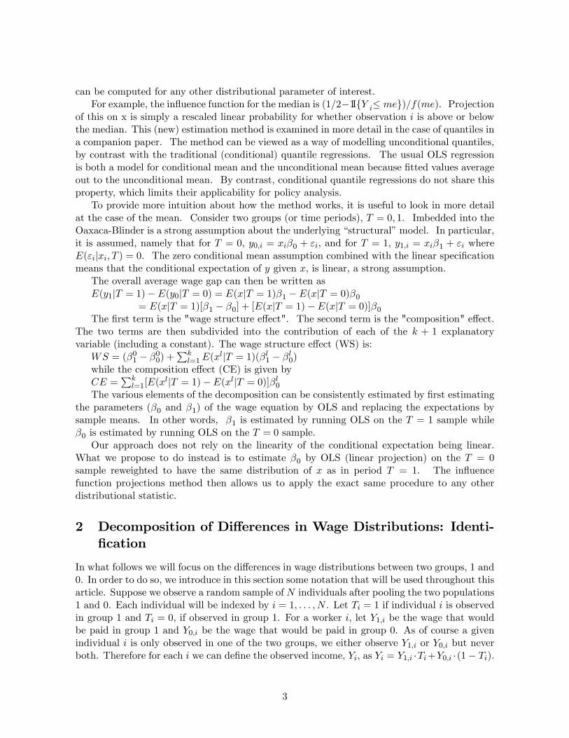
can be computed for any other distributional parameter of interest.For example, the in�uence function for the median is (1=2�1IfY i� meg)=f(me). Projection

of this on x is simply a rescaled linear probability for whether observation i is above or belowthe median. This (new) estimation method is examined in more detail in the case of quantiles ina companion paper. The method can be viewed as a way of modelling unconditional quantiles,by contrast with the traditional (conditional) quantile regressions. The usual OLS regressionis both a model for conditional mean and the unconditional mean because �tted values averageout to the unconditional mean. By contrast, conditional quantile regressions do not share thisproperty, which limits their applicability for policy analysis.

To provide more intuition about how the method works, it is useful to look in more detailat the case of the mean. Consider two groups (or time periods), T = 0; 1. Imbedded into theOaxaca-Blinder is a strong assumption about the underlying �structural�model. In particular,it is assumed, namely that for T = 0, y0;i = xi�0 + "i; and for T = 1, y1;i = xi�1 + "i whereE("ijxi; T ) = 0. The zero conditional mean assumption combined with the linear speci�cationmeans that the conditional expectation of y given x, is linear, a strong assumption.

The overall average wage gap can then be written asE(y1jT = 1)� E(y0jT = 0) = E(xjT = 1)�1 � E(xjT = 0)�0

= E(xjT = 1)[�1 � �0] + [E(xjT = 1)� E(xjT = 0)]�0The �rst term is the "wage structure e¤ect". The second term is the "composition" e¤ect.

The two terms are then subdivided into the contribution of each of the k + 1 explanatoryvariable (including a constant). The wage structure e¤ect (WS) is:

WS = (�01 � �00) +Pkl=1E(x

ljT = 1)(�l1 � �l0)while the composition e¤ect (CE) is given byCE =

Pkl=1[E(x

ljT = 1)� E(xljT = 0)]�l0The various elements of the decomposition can be consistently estimated by �rst estimating

the parameters (�0 and �1) of the wage equation by OLS and replacing the expectations bysample means. In other words, �1 is estimated by running OLS on the T = 1 sample while�0 is estimated by running OLS on the T = 0 sample.

Our approach does not rely on the linearity of the conditional expectation being linear.What we propose to do instead is to estimate �0 by OLS (linear projection) on the T = 0sample reweighted to have the same distribution of x as in period T = 1. The in�uencefunction projections method then allows us to apply the exact same procedure to any otherdistributional statistic.

2 Decomposition of Di¤erences in Wage Distributions: Identi-�cation

In what follows we will focus on the di¤erences in wage distributions between two groups, 1 and0. In order to do so, we introduce in this section some notation that will be used throughout thisarticle. Suppose we observe a random sample of N individuals after pooling the two populations1 and 0. Each individual will be indexed by i = 1; : : : ; N . Let Ti = 1 if individual i is observedin group 1 and Ti = 0, if observed in group 1. For a worker i, let Y1;i be the wage that wouldbe paid in group 1 and Y0;i be the wage that would be paid in group 0. As of course a givenindividual i is only observed in one of the two groups, we either observe Y1;i or Y0;i but neverboth. Therefore for each i we can de�ne the observed income, Yi, as Yi = Y1;i �Ti+Y0;i �(1� Ti).

3

Finally, suppose there is a vector of covariates X 2 X � Rr that we can observe in both groups.Hence, for the individual i we will observe Xi.

Wage determination depends on X and on some unobserved components " 2 Rm throughY1;i = g1(Xi; "i) and Y0;i = g0(Xi; "i), where g1(�; �) and g0(�; �) are unknown real-valued map-pings: for j = 0; 1, gj : Rr�Rm ! R+[f0g:We call each one of those gj (�) functions the wagestructure prevailing at group j. As we are not imposing any distribution assumption or speci�cfunctional form, writing Y1 and Y0 in this way does not restrict the analysis in any sense. Notethat in fact, it may even be the case that for some j in f0; 1g, gj(�; ") = hj("), or in other words,X does not a¤ect the wage structure process for a given group. We will however assume that(T;X; ") have an unknown joint distribution but that is far from being restrictive.

Given sequence to the de�nitions, for a given value x of X, we de�ne the �propensity-score�as the proportion of people in the combined population of two groups that is in group 1, giventhat those people have X = x, that is, p(x) = Pr[T = 1jX = x]. The unconditional proportionof people in group 1 is p which will be assumed to be positive.

Note that from our sample of size N of (Y; T;X) we can estimate the distributions ofY1; XjT = 1 and Y0; XjT = 0, respectively, FY1;XjT (�jT = 1) and FY0;XjT (�jT = 0), or in ashortened notation simply FY1;XjT=1 and FY1;XjT=0: Without further assumptions, we cannothowever estimate the distribution of Y0; XjT = 1, FY0;XjT=1, which is the distribution thatwould have prevailed with the wage structure of group 0 but with individuals from group 1.This distribution will be a counterfactual distribution.

We are interested in analyzing the di¤erence in wage distributions between groups 1 and 0by looking at some �nite parameters of those distributions. Let � be such parameter de�nedas a functional of wage distributions or, more generally, a functional of the conditional jointdistribution of (Y1; Y0; X) jT , that is � : F� ! Rk and F� is a class of distribution functions suchthat F 2 F� if � (F ) < +1 and F (�) is continuously di¤erentiable in the support (Y1; Y0; X) jT ,with positive �rst derivative, f (�). In order to simplify notation, de�ne W1 = [Y1; X

0]0, W0 =[Y0; X

0]0, and W = [Y;X 0]0. The functionals we are interested in are typically �nite vectors ofparameters. However, in a special case, we will also be interested in the density f (y1; y0; xjt),which, given the continuity assumption, will be completely determined by F and, therefore, canbe written as � (F ) with dimension being k = +1.

The di¤erence in the ��s between the two groups is called here the overall wage gap (mea-sured in terms of �) or alternatively, the �-total wage gap, ��O:

��O = ��FW1jT=1

�� �

�FW0jT=0

�(1)

Note that Equation 1 is a simple di¤erence in the parameter �. Interesting examples of thosesimple di¤erences are several. They could be, for example, di¤erence in means (E [Y1jT = 1]�E [Y0jT = 0]), di¤erence in medians, (me (Y1jT = 1)�me (Y0jT = 0)), di¤erence in other quan-tiles, di¤erence in projection coe¢ cients ((E [X �X 0jT = 1])�1�E [X � Y1jT = 1]�(E [X �X 0jT = 0])�1�E [X � Y0jT = 0]). We can use the fact that X is potentially unevenly distributed across groupsand try to control for that by decomposing Equation ��O in two parts:

1

��O =��W1jT=1 � �W0jT=1

�+��W0jT=1 � �W0jT=0

�(2)

The �rst term of the sum is the di¤erence in the parameter � between groups 1 and 0 ifall individuals under consideration were from group 1. This is the e¤ect of changes in the

1We will sometimes refer to the functional �(FZ) simply as �Z :

4

�wage structure�, which is summarized by the functions g1(�; �) and g0(�; �): Therefore this �rstterm corresponds to the e¤ect in � of a change from g1(�; �) to g0(�; �) keeping the distribution(X; ")jT = 1.

The second term corresponds to changes in the distribution of (X; "), keeping the �wagestructure�g0(�; �). In particular, the change is from (X; ")jT = 1 to (X; ")jT = 0. This is oftencalled the composition e¤ect.

Note that unless we impose restrictions on the distributions of (T;X; ") we cannot sayanything about the �rst term re�ecting di¤erences in the wage structure �controlling for theX�s� only. Actually, if we had �xed constant only the distribution of X�s, those di¤erenceswould be confounded by the presence of unobservable components that are part of the wagedetermination. By the same reason, without further restrictions, we cannot say anything aboutthe second term being the composition e¤ect of changes on X only. Again, it will be confoundedby changes in the distribution " across groups as well.

Under identi�cation assumptions however, ��O can be written as the sum of two identi�ablee¤ects, ��S , which corresponds to changes in wage structure keeping the distribution of X �xedas of FXjT=1; and ��C , the composition e¤ect of changing the distribution of X: from FXjT=1to FXjT=0. In order to identify those decomposition terms, we need the following condition tohold:

Assumption 1 Let (T;X; ") have a joint distribution. For all x in X : " is independent of Tgiven X = x:

Some comments on Assumption 1 follow. First, this assumption has become popular in em-pirical research after a series of papers by Rubin and coauthors and by Heckman and coauthors2.In the program evaluation literature, this assumption is sometimes called unconfoundedness andallows identi�cation of the treatment e¤ect on the treated sub-population. Assumption 1 shouldbe analyzed in a case-by-case situation, as for many exercises it is plausible to hold. In our case,it states that the distribution of the unobserved explaining factors of the wage determinationis the same across groups 1 and 0 once we condition on a vector of observed components.

We also make an overlap assumption:

Assumption 2 For all x in X , p(x) < 1: Furthermore, 0 < Pr[T = 1]:

Under Assumption 2 there is overlap in observable characteristics across groups, in the sensethat it does not exist a value of x in X such that it is only observed among people in group 1.

We de�ne three weighing functions that will be very useful in our identi�cation results:

!1(T ) =T

p

!0(T ) =1� T1� p

!0j1(T;X) =

�p(X)

1� p(X)

���1� pp

�� 1� T1� p :

We are now able to state the following result on identi�cation of ��S and ��C :

2See, for instance, Rosenbaum and Rubin (1983 and 1984), Heckman, Ichimura, and Todd (1997) and Heck-man, Ichimura, Smith, and Todd, (1998).

5

Lemma 1 Under Assumptions 1 and 2,(i)

FW1jT=1(w) = E

"!1(T ) �

r+1Yl=1

1IfW l� wlg#

FW0jT=0(w) = E

"!0(T ) �

r+1Yl=1

1IfW l� wlg#

FW0jT=1(w) = E

"!0j1(T;X) �

r+1Yl=1

1IfW l� wlg#

(ii) ��S = �W1jT=1 � �W0jT=1 and ��C = �W0jT=1 � �W0jT=0 are identi�able.

3

At this point, is worth having a simple example for illustration purposes. Consider thedi¤erence in means �Y1jT=1 � �Y0jT=0:

�Y1jT=1 � �Y0jT=0 =��Y1jT=1 � �Y0jT=1

�+��Y0jT=1 � �Y0jT=0

�and let us focus on each part of the previous sum separately:

�Y1jT=1 � �Y0jT=1 = E [g1 (X; ") j T = 1]� E [g0 (X; ") j T = 1]= E [g1 (X; ") j T = 1]� E [E [g0 (X; ") j X;T = 1] j T = 1]

but by Assumption 1:

E [g1 (X; ") j T = 1]� E [E [g0 (X; ") j X;T = 1] j T = 1]= E [g1 (X; ") j T = 1]� E [E [g0 (X; ") j X;T = 0] j T = 1]

and expanding it using integrals:

E [g1 (X; ") j T = 1]� E [E [g0 (X; ") j X;T = 0] j T = 1]

=

Z �Z(g1 (x; �)� g0 (x; �)) dF"jX (� j x)

�dFXjT=1 (x j T = 1)

so it is clear that such di¤erence is attributable only to di¤erences (in a average or mean sense) inthe gj (�)�s. The expression

R(g1 (x; �)� g0 (x; �)) dF"jX (� j x) is the so-called �average partial

e¤ect� at a given level X = x of migrating from group 0 to group 1. Its integral using thedistribution of covariates at T = 1 yields the average wage gap.

Now, going back to previous expression, note that

E [g1 (X; ") j T = 1]� E [E [g0 (X; ") j X;T = 0] j T = 1]= E [Y1 j T = 1]� E [E [Y0 j X;T = 0] j T = 1]

3Note that even if g1(�; ") = h1(") and g0(�; ") = h0(") the result from Lemma 1 is una¤ected. The intuitionis that since (X; ") have a joint distribution, we can use the available information on that distribution to reweighthe e¤ect of the "�s on Y .

6

which from de�nition of Y1 and Y0. Now, using Y = Y1 � T + Y0 � (1� T ):

E [Y1 j T = 1]� E [E [Y0 j X;T = 0] j T = 1]= E [Y j T = 1]� E [E [Y j X;T = 0] j T = 1]

= E�T

p� Y�� E

�E��

1� T1� p (X)

�� Y j X

�j T = 1

�and the last equality follows by using twice the law of iterated expectations and Assumption 2.Now, using the Bayes�rule, the weights de�nition, and dividing and multiplying by 1 � p, wehave:

E�T

p� Y�� E

�E��

1� T1� p (X)

�� Y j X

�j T = 1

�= E [!1(T ) � Y ]� E

�p (X)

p� E��

1� T1� p (X)

�� Y j X

��= E [!1(T ) � Y ]� E

��p (X)

1� p (X)

���1� pp

�� E��1� T1� p

�� Y j X

��= E [!1(T ) � Y ]� E

�!0j1(T;X) � Y

�which proves that �Y1jT=1 � �Y0jT=1, or simply �

�S is expressible in terms of observed data

(Y; T;X).Now, we want to see that and that �Y0jT=1 � �Y0jT=0 can also be identi�ed from the data

and that it re�ects only di¤erences in the distribution (in this case, in a average sense) of theX�s. result. Using the law of iterated expectations and the ignorability assumption:

�Y0jT=1 � �Y0jT=0 = E [g0 (X; ") j T = 1]� E [g0 (X; ") j T = 0]= E [E [g0(X; ") j X;T = 1] j T = 1]� E [E [g0(X; ") j X;T = 0] j T = 1]+ E [E [g0(X; ") j X;T = 0] j T = 1]� E [E [g0(X; ") j X;T = 0] j T = 0]

= E [E [g0(X; ") j X] j T = 1]� E [E [g0(X; ") j X] j T = 1]+ E [E [g0(X; ") j X;T = 0] j T = 1]� E [E [g0(X; ") j X;T = 0] j T = 0]

= 0 + E [E [g0(X; ") j X;T = 0] j T = 1]� E [E [g0(X; ") j X;T = 0] j T = 0]

and since E [g0(X; ") j X;T = 0] is a function of X only, the last expression captures onlydi¤erences in the distributions of XjT = 1 and XjT = 0, �xing the wage structure as the oneof group 0 (by using the g0 (�).function).

A comment on the general result. Non-parametric identi�cation of either the income struc-ture functions g1(�; �) and g0(�; �), or the distribution function of " are not necessary for thee¤ects ��S and �

�C to be identi�ed. Therefore, methods based on conditional mean restrictions

(the Oaxaca-Blinder extension approach) and methods based on conditional quantile restric-tions (the Machado-Mata approach) are based on too strong identi�cation conditions that canbe easily relaxed if the �nal interest is in the terms ��S and �

�C .

We can now turn our attention to estimation and inference. We will consider two separatecases. In the �rst one, the weighting functions are parametrically estimated. In the second case,we estimate those weighting functions non-parametrically, as they will be functions of observed(T;X). In both cases, we derive the distribution theory of �nal estimators.

7

3 Decomposition of Di¤erences in Wage Distributions: Estima-tion and Inference

We proceed in this section in the following way. In subsection 3:1, we discuss how one wouldestimate each of the previous parameters by means of a two-step approach. Then in subsection3:2 we discuss the asymptotic behavior of their estimators.

3.1 First Step Estimation

We now present the estimation procedure for each one of the following three quantities ��FW1jT=1

�;

��FW0jT=0

�and �

�FW0jT=1

�. Note that for the �rst two quantities, estimation is very stan-

dard as the distributions of W1jT = 1 and W0jT = 0 are identi�ed from data on (Y; T;X). Theone that requires special attention is estimation of �

�FW0jT=1

�but that can be dealt with the

reweighing scheme under the ignorability assumption. For implementation of the reweightingprocedure, we need to compute the weighting function. We now present two usual methods todeal with that problem.

3.1.1 Estimating the Weights

We are interested in estimating weights ! that are generally functions of the distribution of(T;X). The three weighting functions under consideration are !1j1(T ), !0j0(T ), and !0j1(T;X).The �rst two weights are trivially estimated by:

b!1j1(T ) =Tbp

b!0j0(T ) =1� T1� bp

where bp = N�1PNi=1 Ti.

The weighting function !0j1(T;X) can be estimated by:

b!0j1(T;X) = 1� T1� bp �

�1� bpbp

��� bp (X)1� bp (X)

�The issue is how to estimate the probability of being in group 1 given X. Consider �rst aparametric approach.

Parametric propensity score estimation Suppose that p (X) is correctly speci�ed up to a�nite vector of parameters �0. That is, p (X) = p (X; �0). Estimation of �0 follows by maximumlikelihood:

b�MLE = argmax�

NXi=1

Ti � log (p (X; �)) + (1� Ti) � log (1� p (X; �))

De�ne, the derivative of p (X; �) with respect to � as�p (X; �) = @p (X; �) =@�. The score

function s (T;X; �) will be:

s (T;X; �) =�p (X; �) � T � p (X; �)

p (X; �) � (1� p (X; �))

8

following a normalization argument, we suppress the entry for � whenever a function of it isevaluated at the true �. Therefore,

s (T;X; �0) = s (T;X) =�p (X) � T � p (X)

p (X) � (1� p (X))

and �nally

b!0j1(T;X) = 1� T1� bp �

�1� bpbp

��

0@ p�X;b�MLE

�1� p

�X;b�MLE

�1A

Nonparametric propensity score estimation Suppose that p (X) is completely unknownto the researcher. In that case, following Hirano, Imbens and Ridder (2003), we approximatethe log odds ratio by a polynomial series. In practice, this is done by �nding a vector b� that isthe solution of the following problem:

�̂ = argmax�

NXi=1

Ti � log�L�HK (Xi)

0 ���+ (1� Ti) � log

�1� L

�HK (Xi)

0 ���

where L : R! R, L(z) = (1+ exp(�z))�1; and HK(x) = [HK; j(x)] (j = 1; :::;K), a vector oflength K of polynomial functions of x 2 X satisfying the following properties: (i) HK : X !RK ; and (ii) HK; 1(x) = 1. If we want HK(x) to include polynomials of x up to the order n,then it is su¢ cient to choose K such that K � (n+1)R. The non-parametric estimation comesfrom the fact that such approximation is re�ned as the sample size increases, that is, K will bea function of the sample size N; K = K(N)! +1 as N ! +1.

In that approach, p(x) is estimated by p̂(x) = L(HK(x)0�̂), thus:

b!0j1(T;X) = 1� T1� bp �

�1� bpbp

���

L(HK(x)0�̂)

1� L(HK(x)0�̂)

�In Appendix we state a set of assumptions that will guarantee uniform convergence of b!(�),

which will be used in deriving the asymptotic properties of our �nal estimators.

3.1.2 Reweighting Estimates of Distributions

We are interested in the estimation and inference of �W1jT=1, �W0jT=0, �W0jT=1 and their di¤er-ences. ��O, �

�S and �

�C . It can be shown that under certain regularity conditions, estimators

of those objects will be distributed asymptotically normally. We now show how to estimatethose quantities and derive their asymptotic distributions for two major cases: �nite vector ofparameters, just called � and the density f (�).

Start with the �nite vector of parameters. Estimation follows by a plug-in approach. Thequantity �Z = � (FZ) is just the functional � evaluated at the distribution FZ . Replacing thec.d.f. by the empirical distribution function produces the estimators of interest: b�Y1jT=1 =

9

�� bFY1jT=1�; b�Y0jT=0 = �

� bFY0jT=0�;b�Y0jT=1 = �� bFY0jT=1� where

bFW1jT=1(w) = N�1NXi=1

b!1(Ti) � r+1Yl=1

1IfW i;l� wlg

bFW0jT=0(w) = N�1NXi=1

b!0(Ti) � r+1Yl=1

1IfW i;l� wlg

bFW0jT=1(w) = N�1NXi=1

b!0j1(Ti; Xi) � r+1Yl=1

1IfW i;l� wlg

To be concrete, consider three examples: the mean �, the medianme, and the variance �2 of theconditional distributions Y1jT = 1, Y0jT = 0 and Y0jT = 1. Starting with the mean: b�Y1jT=1 =N�1PN

i=1 b!1j1(Ti) � Yi; b�Y0jT=0 = N�1PNi=1 b!0j0(Ti) � Yi; and b�Y0jT=1 = N�1PN

i=1 b!0j1(Ti) � Yi.The median will be estimated by: cmeY1jT=1 = argminq

PNi=1 b!1j1(Ti) � jYi � qj; cmeY0jT=0 =

argminqPNi=1 b!0j0(Ti) � jYi � qj; and cmeY0jT=1 = argminqPN

i=1 b!0j1(Ti) � jYi � qj. Finally, the

variance will be: b�2Y1jT=1 = N�1PNi=1 b!1j1(Ti) ��Yi � b�Y1jT=1�2; b�2Y0jT=0 = N�1PN

i=1 b!0j0(Ti) ��Yi � b�Y0jT=0�2; and b�2Y0jT=1 = N�1PN

i=1 b!0j1(Ti) � �Yi � b�Y0jT=1�2.The densities fW1jT (wjt) and fW0jT (wjt) cannot be estimated by the plug-in method using

�� bF� since bF does not have a density and, therefore, � � bF� is not de�ned. However, estimationfollows by a weighted kernel density estimation. Note that three densities of our interest can bede�ned as the following limiting functionals fWj jT (wjt = s) = limh!0

�h�1 � E [Kh (Wj � w) jT = s]

,

where j; s = 0; 1, Kh (�) is a Rr+1 ! R kernel function such that Kh (Wj � w) = h�1 �K�Wj;1�w1

h1;Wj;2�w2

h2; : : : ;

Wj;r+1�wr+1hr+1

�, h =

Qr+1l=1 hl and [h1; : : : ; hr+1]

0 is an r + 1 vector of

bandwidths. The expectations inside the limits can be identi�ed as they are just particu-lar cases of Theorem 1: fWj jT (wjt = s) = limh!0

�h�1 � E

�!jjs(Ti; Xi) �Kh (W � w)

�, for

j; s = 0; 1. The associated estimators are, therefore:

bfW1jT (wjt = 1) = N�1 �NXi=1

b!1j1(Ti) �Kh (Wi � w)

bfW0jT (wjt = 0) = N�1 �NXi=1

b!0j0(Ti) �Kh (Wi � w)

bfW0jT (wjt = 1) = N�1 �NXi=1

b!0j1(Ti; Xi) �Kh (Wi � w)

Such approximation of f (�) by bf (�) is re�ned as the sample size increases, that is, h will be afunction of the sample size N; h = h(N)! 0 as N ! +1.

3.1.3 Asymptotic Distribution

We now show that the plug-in estimators b� are asymptotically normal and compute theirasymptotic variances. We start assuming that the estimators b� are asymptotically linear in thefollowing sense:

10

Assumption 3 (Asymptotic Linearity) If fZ1; Z1; : : : ; ZNg; a random sample of size N

from FZ were available then the plug-in estimator �� bFZ� of � (FZ) could be expressed as

�� bFZ� = � (FZ) +N

�1PNi=1

� (Zi;FZ) + op

�1=pN�, where bFZ (z) = N�1PN

i=1 1IfZi� zg.

There are estimators of functionals of the data distribution that are exactly linear, as thosethat are based on sample moments. There are others that can be linearized and the remainderterm will approach zero as the sample size increases. One example of an estimator in thatclass is the sample median. The in�uence function of the sample median, me is known to be

me (z;FZ) =�dFZ(z)dz jz=me

��1� (1=2� 1Ifz � meg). For the other examples already discussed,

the respective in�uence functions are � (z;FZ) = z � �, for the mean, and �2(z;FZ) =�

z �R� � dFZ (�)

�2 � �2 for the variance,.Under ignorability the estimators b�W1jT=1, b�W0jT=0, and b�W0jT=1, proposed in a previ-

ous section will remain asymptotically linear. We consider two cases: Parametric and non-parametric �rst step:

Theorem 1 (a) Under the above assumptions:

(i)pN �

�b�W1jT=1 � �W1jT=1�= 1p

N

PNi=1 !1j1(Ti) � �

�Yi; Xi;FW1jT=1

�+ op(1)

D! N�0; V1j1

�,

(ii)pN �

�b�W0jT=0 � �W0jT=0�= 1p

N

PNi=1 !0j0(Ti) � �

�Yi; Xi;FW0jT=0

�+ op(1)

D! N�0; V0j0

�(iii) (a) if in addition we assume [parametric], then:

pN �

�b�W0jT=1 � �W0jT=1�=

1pN

NXi=1

!0j1(Ti; Xi) � ��Yi; Xi;FW0jT=1

�+�!1j1(Ti)� !0j1(Ti; Xi)

���p (Xi)

0

p (Xi)��E�s (T;X) � s (T;X)0

���1� E" �

p (X)

1� p (X) � E� ��Y;X;FW0jT=1

�j X;T = 0

�#+ op(1)

D! N�0; V0j1;P

�(iii) (b) otherwise, if in addition we assume [non-parametric], then:

pN �

�b�W0jT=1 � �W0jT=1�=

1pN

NXi=1

!0j1(Ti; Xi) � ��Yi; Xi;FW0jT=1

�+�!1j1(Ti)� !0j1(Ti; Xi)

�� E� ��Y;X;FW0jT=1

�j Xi; T = 0

�+ op(1)

D! N�0; V0j1;NP

�where

V1j1 = Eh�!1j1(T ) � �

�Y;X;FW1jT=1

��2iV0j0 = E

h�!0j0(T ) � �

�Y;X;FW0;XjT=0

��2i

11

V0j1;P = E

" !0j1(T;X) � �

�Y;X;FW0jT=1

�+�!1j1(T )� !0j1(T;X)

���p (X)0

p (X)��E�s (T;X) � s (T;X)0

���1� E" �

p (X)

1� p (X) � E� ��Y;X;FW0jT=1

�j X;T = 0

�#!2#

V0j1;NP = E

" !0j1(T;X) � �

�Y;X;FW0jT=1

�+�!1j1(T )� !0j1(T;X)

�� E� ��Y;X;FW0jT=1

�j X;T = 0

�!2#

The density estimators bfWj jT (wjt = s), j; s = 0; 1 are, for a �xed bandwidth h, exactlylinear. The derivation of the asymptotic distribution of those estimators follows the samestructure of plug-in estimators, but a stronger smoothness condition has to be imposed, sincenow two simultaneous approximations are taking place: the p-score estimation (and the associ-ated smoothness parameter K(N)) and the density estimation (and the associated smoothnessparameter h(N)).

Theorem 2 (a) Under the above assumptions:

(i)pN � h �

� bfW1jT=1 (w)� fW1jT=1 (w)�D! N

��1j1 (w) ; V1j1 (w)

�,

(ii)pN � h �

� bfW0jT=0 (w)� fW0jT=0 (w)�D! N

��0j0 (w) ; V0j0 (w)

�(iii) (a) if in addition we assume [parametric], then:pN � h �

� bfW0jT=1 (w)� fW0jT=1 (w)�D! N

��0j1 (w) ; V0j1;P (w)

�(iii) (b) otherwise, if in addition we assume [non-parametric], then:pN � h �

� bfW0jT=1 (w)� fW0jT=1 (w)�D! N

��0j1 (w) ; V0j1;NP (w)

�where

V1j1 (w) = fW1jT=1 (w) �Z(K (u))2 du

V0j0 (w) = fW0jT=0 (w) �Z(K (u))2 du

V0j1;P (w) = E

" !0j1(T;X) �Kh (W � w)

+�!1j1(T )� !0j1(T;X)

���p (X)0

p (X)��E�s (T;X) � s (T;X)0

���1� E" �

p (X)

1� p (X) � E [Kh (W � w) j X;T = 0]#!2#

12

V0j1;NP (w) = E

" !0j1(T;X) �Kh (W � w)

+�!1j1(T )� !0j1(T;X)

�� E [Kh (W � w) j X;T = 0]

!2#

and

�1j1 (w) =h2

2tr

�Zuu0K (u) du

��@2fW1jT=1 (w)

@w@w0

!

�0j0 (w) =h2

2tr

�Zuu0K (u) du

��@2fW0jT=0 (w)

@w@w0

!

�0j1 (w) =h2

2tr

0@�Z uu0K (u) du

��@2�fW1jT=1 (w) �

p(x)p�(1�p(x))

�@w@w0

1A

3.1.4 Variance Estimation

We now show how to estimate the asymptotic variance of estimators that we have presentedso far. We then state some su¢ cient conditions for that estimator to be consistent. The fourobjects that we need to estimate are V1j1, V0j0, V0j1;P and V0j1;NP . Respective estimation ofV1j1and V0j0 follows trivially by:

bV1j1 = N�1NXi=1

�b!1j1(Ti) � b � �Yi; Xi; bFW1jT=1

��2bV0j0 = N�1

NXi=1

�b!0j0(Ti) � b � �Yi; Xi; bFW0jT=0

��2where b � (�; �) is a consistent estimator of � (�; �). For example, for the median of Y1jT = 1,

we would use b me �y; bFY1jT=1� = � bfY1jT=1 �cmeY1jT=1���1 � (1=2 � 1Ify � cmeY1jT=1g) wherebfY1jT=1 (�) is a consistent estimator for the density of Y1jT = 1, fY1jT=1 (�).Estimation of both V0j1;P and V0j1;NP are more complex as they involve in both cases

estimation of E� ��Y;X;FW0jT=1

�j X;T = 0

�. We propose estimating that by:

bE � � �Y;X;FW0jT=1�j X;T = 0

�= HK (X)

0 b where

b = NXi=1

b!0j0(Ti) �HK(Xi) �HK(Xi)0!�1

�NXj=1

b!0j0(Tj) �HK(Xj) � b � �Yj ; Xj ; bFW0jT=1

�

13

Thus:

bV0j1;P = N�1NXi=1

b!0j1(Ti; Xi) � b � �Yi; Xi; bFW0;XjT=1

�+�b!1j1(Ti)� b!0j1(Ti; Xi)� �

�p�Xi;b��0

p�Xi;b��

�

0@ NXj=1

s�Tj ; Xj ;b�� � s�Tj ; Xj ;b��0

1A�1 � NXl=1

�p�Xl;b��0

1� p�Xl;b�� �HK (Xl)0 b

!2

and

bV0j1;NP = N�1NXi=1

b!0j1(Ti; Xi)�b � �Yi; Xi; bFW0;XjT=1

�+�b!1j1(Ti)� b!0j1(Ti; Xi)��HK (Xi)0 b

!2

Theorem 3 : (Consistent Estimation of the Asymptotic Variance): Under the aboveassumptions, bV�� � V�� = op(1).

3.2 Second Step: In�uence Function Projections

Let�s �rst illustrate how the second step of our estimation procedure works in the case of themean, where we have

�W1jT=1 = E(Y1jX;T = 1), �W0jT=0 = E(Y0jX;T = 0), and �W0jT=1 = E(Y0jX;T = 1):Estimates b� of the ��s are obtained by computing sample means of Y using the three

estimated weights b!1, b!0 and b!1j0. For example,bE(Y1jX;T = 1) =PNi=1 b!1(Ti)Yi:

Now consider the three sets of projection coe¢ cients:

b 1 =

NXi=1

b!1(Ti)XiXi0!�1 � NXi=1

b!1(Ti)XiYib 0 =

NXi=1

b!0(Ti)XiXi0!�1 � NXi=1

b!1(Ti)XiYib 0j1 =

NXi=1

b!0j1(Ti; Xi)XiXi0!�1

�NXi=1

b!0j1(Ti; Xi)XiYiBy de�nition, it follows thatb�W1jT=1 =

bE [X;T = 1] b 1, b�W0jT=0 =bE [X;T = 0] b 0, andb�W0jT=1 =

bE [X;T = 1] b 0j1.We can thus rewrite the decomposition for the mean as:

b��O =

� bE [X;T = 1] b 1 � bE [X;T = 1] b 0j1�+� bE [X;T = 1] b 0j1 � bE [X;T = 0] b 0�

14

This is very similar to the standard Oaxaca-Blinder decomposition except that the counter-factual mean wage is bE [X;T = 1] b 0j1 instead of bE [X;T = 1] b 0 in the standard decomposition.This di¤erence between b 0j1 and b 0 is linked to the Shortcoming 2 of the standard decompo-sition mentioned above. We later show an empirical example where this di¤erence turns outto be quite important

Let �(Y ) be the in�uence function for the mean, where �(Y ) = Y � �. Consider therescaled in�uence function

��(Y ) = �+ �(Y ) = Y .In the case of the median, the rescaled in�uence function is�me(Y ) = me+ (1=2� 1IfY � meg)=f(me).More generally, the rescaled in�uence function of the qth quantile yq is�q(Y ) = yq + (q � 1IfY � yqg)=f(yq).The rescaled in�uence function can be computed for each observation by plugging the sample

estimate of the quantile, byq, and estimating the density at the sample quantile, bf(byq).Since the rescaled in�uence function is equal to Y in the case of the mean, the projections

used above turn out to be projection of the rescaled in�uence functions on X. By analogy,rescaled in�uence function for other distributional parameters such as quantiles can also beprojected on X. For example, for the qth quantile we have:

b q1 =

NXi=1

b!1(Ti)XiXi0!�1 � NXi=1

b!1(Ti)Xib�q1(Yi)b q0 =

NXi=1

b!0(Ti)XiXi0!�1 � NXi=1

b!1(Ti)Xib�q0(Yi)b q0j1 =

NXi=1

b!0j1(Ti; Xi)XiXi0!�1

�NXi=1

b!0j1(Ti; Xi)Xib�q1j0(Yi)We can thus decompose this quantile as:b�qO =

� bE [X;T = 1] b q1 � bE [X;T = 1] b q0j1�+� bE [X;T = 1] b q0j1 � bE [X;T = 0] b q0�

This generalizes the Oaxaca-Blinder decomposition to any quantile. The same techniquecan also be used to decomposition standard distributional measures like the variance or theGini coe¢ cient.

4 Empirical Applications

We use di¤erent empirical applications to illustrate various features of our decompositionmethod. We focus on three particular issues The �rst issue we look at the issues we lookat in this section are:

1. Illustrate speci�cation problems in the standard decomposition by running Mincer wageequations for men in 1973 and 2003

15

2. Show how in�uence function projection work by looking at the e¤ect of unions on wagesby quantiles of the wage distribution (and contrast with traditional quantile regressions

3. Decompose 1973-2003 changes in wage inequality (variance and 90-10 gap).

4.1 Mispeci�cation of a Mincer-type wage equation

Table 2 shows standard estimates of a Mincer wage equation for men in 1973 and 2003. The1973 data are from the May Supplement of the Current Population Survey (CPS). The 2003data are from the Outgoing Rotation Groups (ORG) Supplement of the CPS. More detail onthe these data is provided in Lemieux (2005). We both report the most standard version of theMincer equation where log wages are regressed on a linear function of years of education and aquadratic function of potential experience, as well as a extended speci�cation where a quarticspeci�cation in experience is used (as in Murphy and Welch, 1990).

The Mincer equation is an interesting case to explore because there is growing evidence thatthe e¤ect of education on wages has become more and more convex over time (Deschenes, 2002,Mincer 1997). This is thus a prime case where the simple linear speci�cation is likely incorrect,and where the estimates from a linear speci�cation may well depend on the distribution ofcharacteristics. For example, since the level of education has increased substantially over time,estimating the Mincer equation by OLS in 2003 should yield a larger e¤ect of education on wageswhen the 2003 distribution of characteristics is used than when the 2003 data is reweighted toget the same distribution of characteristics as in 1973.

Table 1 shows that this is indeed what happens. For example, in the models with quadraticexperience (columns 1 to 3), the return to education increase from 0.068 in 1973 to 0.111 in2003, a 0.043 increase. Column 3 shows estimates from a model in which the 2003 data hasbeen reweighted to the 1973 distribution of education and experience.4 In terms of the previousnotation, the coe¢ cients in columns 3 are b 0j1 (T=0 for 2003, T=1 for 1973) compared to b 0for column 2. The returns to education decreases from 0.111 to 0.101, which represents abouta quarter of the increase between 1973 and 2003. This means that using a linear speci�cationfor education overstates the increase in the "price" of education because the true conditionalexpectation function is convex and the level of education is higher in 2003 than in 1973. Interms of a Oaxaca-Blinder decomposition, this means that the decomposition would attributeto changes in the regression coe¢ cients (i.e. to �price e¤ects�) a component linked to mis-speci�cation of the conditional expectation function. Our alternative decomposition �corrects�for this problem by using b 0j1 instead of b 0. The results with the quartic speci�cation forexperience (columns 4 to 6) are very similar.

There is a much smaller change in the return to experience than in the return to education.For example, the coe¢ cient on the linear term increases from 0.042 in 1973 to 0.046 in 2003.Reweighting actually reduces the coe¢ cient instead to 0.038. Figure 2 shows that the samepattern of results holds for the whole experience pro�le. This means that the whole increase inthe experience pro�le (and even more) is a spurious consequence of the fact that 1) the simpleMincer equation is mispeci�ed in 2003, and 2) the distribution of characteristics change in sucha way that the linear approximation becomes steeper than in 1973 (just like �tting the modein Figure 1 for higher values of X yields a steeper regression curve).

4Reweighting is performed by estimating a logit with a full set of esperience and education dummies, plus aset of interactions between education dummies and a quartic in experience.

16

We conclude from this �rst example that mispeci�cation problems can substantially biasthe standard Oaxaca-Blinder decomposition.

4.2 In�uence Function Projections

To illustrate how the in�uence function projections work in practice, we focus on the impact ofunion on wages (for men) which is well known to have a di¤erential impacts at di¤erent pointsin the wage distribution (Card (1996)). There are several reasons for this. First, union bothincrease the conditional mean of wages (the �between�e¤ect) and decrease the conditional dis-tribution of wages. This means that unions tend to increase wages in low wage quantiles whereboth the between and within group e¤ects go in the same direction, but can decrease wages inhigh wage quantiles where the between and within group e¤ects go in opposite directions. Thisis compounded by the fact that the union wage gap generally declines for higher that lowerskills levels.

Table 2 shows detailed estimates of in�uence function projections at the 10th, 50th and 90th

quantiles using 1984 ORG CPS data for men. The results are also compared with the OLSbenchmark. Interestingly, the e¤ect of unions �rst increase from 0.203 at the 10th quantileto 0.339 at the median before turning negative (-0.124) at the 90th quantile. Notice also howthe e¤ect of education changes at the di¤erent quantiles. For example, the e¤ect of post-graduate education (relative to high school) increases from 0.143 at the 10th quantile, to 0.512at the median and 0.880 at the 90th quantile. Since both high school graduates and collegepost-graduates are relatively unlikely to be in the lowest ten percent of the wage distribution,post-graduate education has relatively little e¤ect. By contrast, post-graduate education greatlyincreases the probability of earning above the 90th quantile, thus explaining the much largercoe¢ cient at this quantile.

Table 3 contrast the e¤ect of unions in our in�uence function projections to standard esti-mates based on (conditional) quantile regressions. Remember the key di¤erence between thetwo methods. The in�uence function projections indicate the impact of unions (in this case) onthe unconditional quantiles of wages, while quantile regressions indicate the impact of unionson conditional quantiles. The quantile regression estimates in the second of Table 3 show, asexpected, that unions increase the location of the conditional wage distribution (i.e. positivee¤ect on the median) but also reduce conditional wage dispersion. This explains why the e¤ectof unions monotonically declines as quantiles increase. One cannot infer from the quantile re-gressions, however, what is the overall e¤ect of unions on the unconditional wage distribution.The key problem is that, unlike conditional means, conditional quantiles do not aggregate upto unconditional quantiles. For example, the fact that unions increase the conditional medianby 0.196 does not say anything about the e¤ect of unions on the unconditional median.

In fact, the �rst row of Table 3 show that the e¤ect of unions on unconditional quantilesestimated using our in�uence function projections are quite di¤erent from the conditional quan-tile estimates. For instance, the e¤ect on the median (0.339) largely exceed the conditionalquantile regression estimate of 0.196. Furthermore, the e¤ect is a non-monotonic function ofquantiles. The e¤ect �rst increases from 0.054 at the 5th quantile to 0.374 at the 25th quantilebefore declining to eventually reach a large negative e¤ect of -0.229 at the 95th quantile. Thelarge e¤ect at the top end re�ects the fact that compression e¤ects dominate everything elseat the top end. Union wages are more compressed and do not exhibit the �fat�upper tail ofthe non-union wage distribution. As a result, unions have large and negative impact on theprobability of earning less more than the 95th quantile.

17

The story for the lowest quantiles is a bit di¤erent. In 1984, the 5th quantile turns outto exactly be the minimum wage of $3.35. The wage density is quite high because of thebunching at the minimum wage, which explains why estimated coe¢ cients are relatively small(the inverse of the density appears in the equation for the in�uence function). Intuitively, theidea is that unions and other wage determination variables have little impact at the bottom ofthe wage distribution because everybody is bunched up at the minimum wage anyway.

4.3 Decomposing 1973-2003 changes in the wage distribution

We �nally show in Table 4 how our two step procedure can be used to decompose four parame-ters, the mean, the median, the variance and the 90-10 gap, of the wage distribution between1973 and 2003. The date used are once again the May 1973 and the 2003 ORG CPS for men.The �rst step estimates are obtained by �tting the logit model discussed above to reweightthe 2003 wage distribution. The second step estimates are obtained by running the in�uencefunction projections on a set of education (six) and experience dummies (nine). Instead of re-porting the elements of the decomposition for each dummy, we sum up the e¤ects for educationand experience.

In the case of the mean, remember that the (rescaled) in�uence function is simply ��(Y ) =Y . In the case of the variance we have ��

2(Y ) = (Y � �)2. The in�uence function for the

median is de�ned earlier while the one of the 90-10 gap is just the di¤erence between the twocorresponding in�uence functions:

�90�10(Y ) = �:9(Y )��:1(Y ) = (y:9�y:1)+(:9�1IfY � y:9g)=f(y:9)�(:1�1IfY � y:1g)=f(y:1):The results in column 1 and 2 show that the small decline in the mean and the larger decline

in the median are due to the o¤setting impact of wage structure and composition e¤ects. Forexample, the large secular increase in educational achievement should have resulted in a 0.174increase in the mean and 0.248 increase in the median. This was more than o¤set by thegeneral decline in wages (wage structure e¤ects).

To the best of you knowledge, no Oaxaca-Blinder type decomposition for the median (incolumn 2) have ever been reported in the literature. This illustrates the usefulness of ourprosed method since the median is a fairly standard distributional parameters. The medianis also of particular policy interest since policy measures may or may not be supported by amajority of the population depending on the impact on the median.

Finally, the results of columns 3 and 4 con�rm existing �ndings about the sources of changesin wage inequality. Both wage structure and composition e¤ects (Lemieux, 2005) are important.Changes in returns to education are also a more important component of changes in the wagestructure than changes in returns to experience.

18

REFERENCES

Abadie, A., (2005), �Semiparametric Di¤erence-in-Di¤erences Estimators,�Review of Eco-nomic Studies.

Bishop, J., J. Formby, and P. Thistle, (1992) �Convergence of the South and Non-SouthIncome Distributions, 1969-1979,�The American Economic Review, Vol. 82, No. 1., pp.262-272.

Blinder, A., (1973), �Wage Discrimination: Reduced Form and Structural Estimates,�Jour-nal of Human Resources, 8, 436-455.

Bourguignon, F., F. Ferreira, P. Leite, (2002) �Beyond Oaxaca-Blinder: accountingfor di¤erences in household income distributions across countries�PUC-Rio, TD #452.

Cramér, (1946)

Cowell, F., (1995), Measuring Inequality. (2nd edition). Harvester Wheatsheaf, HemelHempstead.

DiNardo, J., (2002), �Propensity Score Reweighting and Changes in Wage Distributions�,Unpublished paper, University of Michigan, Department of Economics.

DiNardo, J., N. Fortin, and T. Lemieux, (1996), �Labor Market Institutions and theDistribution of Wages, 1973-1992: A Semiparametric Approach,�Econometrica, 64, 1001-1044.

Ferguson, T., (1996), A Course in Large Sample Theory,

Firpo, S. (2004), �E¢ cient Semiparametric Estimation of Quantile Treatment E¤ects,�UBCDepartment of Economics Discussion Paper, No. 04-01.

Heckman, J., H. Ichimura, and P. Todd, (1997), �Matching as an Econometric EvaluationEstimator,�Review of Economic Studies, 65(2), 261-294.

Heckman, J., H. Ichimura, J. Smith, and P. Todd, (1998), �Characterizing SelectionBias Using Experimental Data,�Econometrica, 66, 1017-1098.

Hirano, K., G. Imbens, and G. Ridder, (2003), �E¢ cient Estimation of Average Treat-ment E¤ects Using the Estimated Propensity Score,�forthcoming, Econometrica.

Hoeffding, W., (1948)

Juhn, C., K. Murphy, and B. Pierce, (1993), �Wage Inequality and the Rise in Returnsto Skill,�The Journal of Political Economy, 101, 410-442.

Koenker, R., and G. Bassett, (1978), �Regression Quantiles,�Econometrica, 46, 33-50.

Lehmann, E., (1998), Elements of Large Sample Theory.

Lemieux, T., (2002), �Decomposing Changes in Wage Distributions: a Uni�ed Approach,�The Canadian Journal of Economics, 35, 646-688.

19

Machado, J. and J. Mata, (2004), �Counterfactual Decomposition of Changes in WageDistributions Using Quantile Regression�, Journal of Applied Econometrics, (forthcom-ing).

Newey, W., (1995), �Convergence Rates for Series Estimators,�in Advances in Econometricsand Qualitatice Economics: Essays in Honor of C.R. Rao, G. Maddal, P.C. Phillips, andT.N. Srinivasan, eds., Cambridge US, Basil-Blackwell.

Newey, W., (1997), �Convergence Rates and Asymptotic Normality for Series Estimators,�Journal of Econometrics, 79, 147-168.

Oaxaca, R., (1973), �Male-Female Wage Di¤erentials in Urban Labor Markets,� Interna-tional Economic Review, 14, 693-709.

Rosenbaum, P., and D. Rubin, (1983), �The Central Role of the Propensity Score inObservational Studies for Causal E¤ects,�Biometrika, 70, 41-55.

van der Vaart, A., (1998), Asymptotic Statistics.

Wand, M. and M. Jones, (1994), Kernel Smoothing. Chapman & Hall/CRC.

20

Figu

re 1

: Mis

peci

fied

Con

ditio

nal E

xpec

tatio

n Fu

nctio

n

0.00

1.00

2.00

3.00

4.00

5.00

6.00

00.

20.

40.

60.

81

1.2

1.4

1.6

1.8

2

X va

riabl

e

Y variable

Con

ditio

nal

expe

ctat

ion

Line

ar re

gres

sion

fit

over

dis

tribu

tion

of X

at T

=0 (X

~U(0

,1))

A

B C

Figu

re 2

: Exp

erie

nce

prof

iles

estim

ated

in th

e 19

73 a

nd 2

003

CPS

0.00

0.10

0.20

0.30

0.40

0.50

0.60

0.70

0.80

05

1015

2025

3035

40

Year

s of

exp

erie

nce

Return to experience

2003

1973

2003

rew

eigh

ted

to19

73 d

istri

butio

n of

X

Tabl

e 1:

Min

cer e

quat

ions

for m

en, 1

973

and

2003

1973

2003

2003

1973

2003

2003

rew

eigh

ted

rew

eigh

ted

Edu

catio

n0.

068

0.11

10.

101

0.06

90.

113

0.10

3(0

.001

)(0

.001

)(0

.001

)(0

.001

)(0

.001

)(0

.001

)

Exp

erie

nce

0.04

20.

046

0.03

80.

087

0.08

00.

073

(0.0

01)

(0.0

01)

(0.0

00)

(0.0

03)

(0.0

03)

(0.0

02)

Exp

er^2

-0.0

68-0

.080

-0.0

55-0

.402

-0.2

93-0

.248

(/100

)(0

.002

)(0

.001

)(0

.001

)(0

.026

)(0

.023

)(0

.017

)

Exp

er^3

0.08

20.

041

0.02

8(/1

000)

(0.0

08)

(0.0

08)

(0.0

05)

Exp

er^4

-0.0

06-0

.002

0.00

0(/1

0000

)(0

.001

)(0

.001

)(0

.001

)

Table 2: OLS vs Infuence function projections, 1984 CPS

Influence function projectionsOLS 10th 50th 90th

(1) (2) (3) (4)

Union 0.184 0.203 0.339 -0.124(0.003) (0.006) (0.005) (0.007)

Nonwhite -0.132 -0.126 -0.154 -0.103(0.005) (0.008) (0.007) (0.010)

Married 0.137 0.201 0.150 0.042(0.004) (0.006) (0.005) (0.008)

Educ 0-8 -0.353 -0.303 -0.469 -0.261(0.007) (0.011) (0.010) (0.014)

Educ 9-11 -0.188 -0.355 -0.194 -0.074(0.005) (0.008) (0.007) (0.010)

Educ 13-15 0.131 0.052 0.173 0.161(0.004) (0.007) (0.006) (0.009)

Educ 16 0.409 0.201 0.472 0.599(0.005) (0.008) (0.007) (0.010)

Educ 17+ 0.476 0.143 0.512 0.880(0.005) (0.009) (0.008) (0.011)

Exper 0-4 -0.547 -0.599 -0.639 -0.455(0.006) (0.011) (0.010) (0.014)

Exper 5-9 -0.263 -0.078 -0.356 -0.375-0.006 -0.010 -0.009 -0.013

Exper 10-14 -0.146 -0.037 -0.186 -0.250(0.006) (0.010) (0.009) (0.013)

Exper 15-19 -0.056 -0.026 -0.074 -0.081(0.006) (0.011) (0.010) (0.014)

Exper 25-29 0.036 0.003 0.038 0.078(0.007) (0.012) (0.011) (0.015)

Exper 30-34 0.039 0.000 0.034 0.082(0.007) (0.012) (0.011) (0.016)

Exper 35-39 0.041 0.021 0.029 0.073(0.008) (0.013) (0.012) (0.016)

Exper 40+ 0.010 0.041 0.006 -0.030(0.008) (0.013) (0.012) (0.016)

Tabl

e 3:

Com

parin

g un

ion

effe

ct in

influ

ence

func

tion

and

quan

tile

regr

essi

on m

odel

5th

10th

25th

50th

75th

90th

95th

Influ

ence

func

tion

0.05

40.

203

0.37

40.

339

0.07

4-0

.124

-0.2

29re

gres

sion

s(0

.003

)(0

.006

)(0

.006

)(0

.005

)(0

.005

)(0

.007

)(0

.011

)

Qua

ntile

0.30

90.

295

0.26

10.

196

0.14

00.

095

0.06

9re

gres

sion

s(0

.007

)(0

.003

)(0

.001

)(0

.001

)(0

.004

)(0

.006

)(0

.005

)

Not

e: E

stim

ated

usi

ng 1

984

CP

S d

ata.

Oth

er re

gres

sors

are

the

sam

e as

in T

able

2.

Table 4: Decomposition of 1973-2003 changes in wage distribution

Mean Median Variance 90-10

Overall 1973-2003 change -0.030 -0.067 0.109 0.252

Wage structure effect -0.241 -0.314 0.064 0.109 Education 0.042 0.012 0.033 0.065 Experience 0.012 -0.011 -0.011 0.007 Constant -0.295 -0.315 0.041 0.037

Composition effect 0.211 0.247 0.045 0.143 Education 0.174 0.248 0.006 0.018 Experience 0.027 0.033 0.032 0.078 Constant 0.009 -0.034 0.007 0.047

Note: First-step model estimated using logit model with full set of experience and education dummies, plus interaction between quarticin experience and education dummies. Second step model estimatedusing dummies for 6 education categories and 9 experience categoriesshown in Table 2. Omitted group is high schol graduates with 20-24years of experience. The "experience" and "education" effects in thetable are the sum of the effects for education and experience dummies.