applied sciences

Article

Decision Support Simulation Method for ProcessImprovement of Intermittent Production Systems

Péter Tamás ID

Faculty of Mechanical Engineering and Informatics, Institute of Logistics, University of Miskolc,3515 Miskolc-Egyetemváros, Hungary; alttpeti@gmail.com; Tel.: +36-(70)-409-5713

Received: 20 August 2017; Accepted: 13 September 2017; Published: 15 September 2017

Abstract: Nowadays production system processes are undergoing sweeping changes. The trendsinclude an increase in the number of product variants to be produced, as well as the reduction ofthe production’s lead time. These trends were induced by new devices of the industry’s 4.0, namelythe Internet of Things and cyber physical systems. The companies have been applying intermittentproduction systems (job production, batch production) because of the increase in the number ofproduct variants. Consequently, increasing the efficiency of these systems has become especiallyimportant. The aim of development in the long term—not achievable in many cases—is the realizationof unique production, with mass production’s productivity and lower cost. The improvementof complex production systems can be realized efficiently only through simulation modeling.A standardized simulation method for intermittent production systems has not been elaborated so far.In this paper, I introduce a simulation method for system improvement and present its applicationpossibilities and a practical example.

Keywords: intermittent production system; simulation; process improvement; investigational method

1. Introduction

Continuous improvement of production processes based on customer demands is necessary inorder to increase or maintain competitiveness. The only companies that can stay competitive in the longterm are those that are able to carry out continuous improvements and adapt to external environmentalchanges in all the companies’ areas [1]. If we take into consideration the sweeping changes in thetransformation of production systems in the last 50 years and the developmental possibilities thatarise from the technological progress, we can see that process improvement is a very importantresearch area [2]. The general trends are the satisfaction of unique customer demands, as well asa reduction in production lead time [3,4]. These trends create some new challenges that can only beovercome with intensive improvement of intermittent production systems. Process improvement canrefer to the production systems to be realized. Intermittent production systems are especially complexbecause in the material flow routes for products/product families the technological equipment’soperation time and changeover time often differ, as do the applied unit load making devices [4,5].In practice, improvement can be realized by using the lean philosophy’s device system [5,6]. However,the application of simulation modeling technology is becoming more prominent because of theprocessing’s increasing complexity and developmental demand. We can explain simulation as a methodfor making a computer model on the basis of the real/planned systems; consequently, we examinethese systems’ status changes [3]. We can classify the simulation models according to several aspects.If the simulation model’s input data contain stochastic variables, we can speak about a stochasticsimulation model; otherwise, the simulation model is deterministic [7].

We can distinguish discrete and continuous simulation models on the basis of anotherclassification aspect. The system’s status will be changed in the discrete points of time in the case of the

Appl. Sci. 2017, 7, 950; doi:10.3390/app7090950 www.mdpi.com/journal/applsci

Appl. Sci. 2017, 7, 950 2 of 16

discrete model and at every point of time in the case of the continuous model [8,9]. Basically, the discretesimulation models are used for the production areas [10,11]. Simulation modeling has been applied inboth continuous production systems [12,13] and intermittent production systems (for example: processimprovement [14], production scheduling [10], etc.). Besides the examination of production systems,simulation modeling has been applied in other areas as well (for example: disaster logistics [15],port logistics [16], air circulation in a tennis hall [17], and electric distribution [18]). The objective of thesimulation examinations can be the determination of selected system parameters at different modelsettings [19,20], simulation examination of real-time systems [21–23], or optimizing the workingsof assigned systems [24,25] for intermittent manufacturing systems. Such examinations have beencarried out by discrete event controlled simulation modeling [19–25] or Petri nets [26–29]. Discreteevent controlled simulation modeling has become increasingly important due to its applicabilityand flexibility. However, the studies have only examined the production processes of one productfamily (in which the examined products’ material flow routes are the same) and/or containseveral simplifications.

These studies do not explain how we can create a simulation investigational model in the case ofthe most complex intermittent manufacturing systems. There is a need for a simulation investigationalmodel for intermittent production systems that is able to analyze the logistical processes of more thanone product family simultaneously, where the parameters of the logistical processes can differ fromeach other (e.g., operation times, changeover times, batch sizes, or types of the unit load formingdevices), as well as having numerous material flow nodes and backflows. The ability to model suchsystems is very important because the complexity of manufacturing systems will increase in the futureas a result of the diversification of customer needs.

We have carried out numerous research projects [6,30–32] in recent years and have gaineda great deal of experience in simulation modeling technology. I have elaborated a general simulationinvestigational method based on our experience that is able to examine the operation of even the mostcomplex intermittent production systems. Here I introduce the applied framework’s most importantcharacteristics and the elaborated simulation method for the making of the simulation examination,present the method’s application possibilities, and give a short example related to an intermittentmanufacturing system. I wanted to introduce the investigational method’s working with real companydata as well, but it was not possible due to confidentiality obligations.

2. Introduction of the Applied Simulation’s Framework

We applied the Plant Simulations’ framework 10.1 for the elaborated simulation investigationalmethod. This framework was made by Siemens PLM Software. Naturally the elaborated investigationalmethod can be applied to other simulation frameworks as well (for example: simul8, arena, etc.).

The applied framework most important characteristics are [33]:

• Discrete event-controlled operation: The framework enables the model’s fast running becausethe software will only examine the next important event (for example: arrival of a truck, makinga product, etc.).

• Object-oriented approach: The framework contains predefined objects whose behavior can beset with predefined input data columns in most events (we can use the simtalk programminglanguage if necessary).

• Graphical display possibility: There are numerous types of diagrams and functions for displayingthe created model’s output data.

• Animation display possibility: We can also execute the created simulation models with the useof animation.

• Interactive working: Modification of the input data is possible while the simulation is running(the simulations’ operation will change because of the modification).

Appl. Sci. 2017, 7, 950 3 of 16

• Connection possibility to external databases: We can connect the simulations’ framework toexternal databases (for example: Oracle, SQL, ODBC, XML, etc.).

The simulation framework’s most important structural elements are:

• Class library: This element contains all the objects for making the simulation model. The classlibrary’s one object name is “class,” which object parameters can modify arbitrarily, as well ascreating new classes (by copy or inheritance).

• Toolbox: This element enables faster access to the objects. These objects exist in the class library aswell. Consequently, there is a close link between the toolbox’s and the class library’s objects.

• Modeling area: Actually, a simulation model can be made in a “frame” (the “frame” is a modelingarea for the simulation model). We can create several frames within a frame (in horizontal and/orvertical structures) to enhance transparency (for example: if we have to make a simulation modelof a manufacturing plant we can use a frame for the raw material warehouse, another frame forthe production system and so on).

• Console: We can gain some information about the current status of the simulation model objectswhile the simulation model is running (for example: values of variables, failure messages, etc.).

3. Simulation of Investigational Method for Intermittent Manufacturing Systems

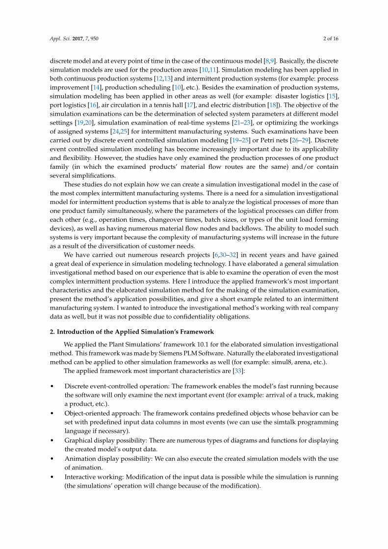
There are numerous possibilities to improving a production system’s logistics processes(for example: reduction of changeover time, reduction of operation time, installation of newtechnological equipment, etc.). However, their effects are difficult to forecast in the case of intermittentmanufacturing systems. In practice, it may be that an intended improvement will not reach itsaim (predefined productivity, etc.), which can lead to unsatisfied customer demands. In addition,the long-term examination of improvement possibilities can result in a competitive disadvantage.We introduce here the steps for a simulation of investigational method for performing more efficientintermittent production system examinations. With improvement, decision lead time can be decreasedand efficiency can be increased. Figure 1 shows the elaborated simulation investigational model’s steps.

Step 1. Determination of the simulation examination’s aims: There can be numerous objectivesregarding the simulation examination of the production systems:

• Elimination of planning failure.• Comparison of planning alternatives.• Determination of the logistics system’s capability.• Comparison of the management strategy versions.• Determination of the more efficient production program.• Examination of the planned development’s effects, etc.

Step 2. Definition of the examined system: We have to define the examined system’s boundaries(for example: a production line, total production system, etc.).

Step 3. Investigation of the system working: After the examined system’s boundaries have beendefined, the simulation model maker has to become familiar with material and information flowfeatures of the examined logistics system.

Step 4. Realization of simulation model of the material flow system: We have to create theexamined material flow system’s simulation model (this model does not contain the moveable unitsand unit load making devices), taking into consideration the following. We can simplify the modelingprocess using standardized objects. Thus, we have elaborated a technological operation object thatis able to realize all operation types. We suggest using the simulation model’s predefined objects fortransportation and warehousing tasks. We can create a basic model with the location of the necessaryobjects and creation of the material flow relation. We have to complement the simulation model withthe Plant Simulation’s objects in those cases where we need to carry out special tasks such as human

Appl. Sci. 2017, 7, 950 4 of 16

work or special material handling activities. The essential objects of the material flow system to becreated are as follows.Appl. Sci. 2017, 7, 950 4 of 17

Figure 1. Steps of the simulation investigation method of intermittent manufacturing systems.

(1). Technological objects class: We can distinguish four types of technological operations in an intermittent production system:

• Single operation: This technological workplace makes an operation on one product in a work cycle (for example: screw driving, turning, drilling, etc.).

• Parallel operation: This technological workplace makes an operation on several products in a work cycle (for example: heat treatment, painting, etc.).

• Assembly operation: This technological workplace makes one product out of several products in a work cycle.

• Disassembly operation: This technological workplace makes several products from one product in a work cycle.

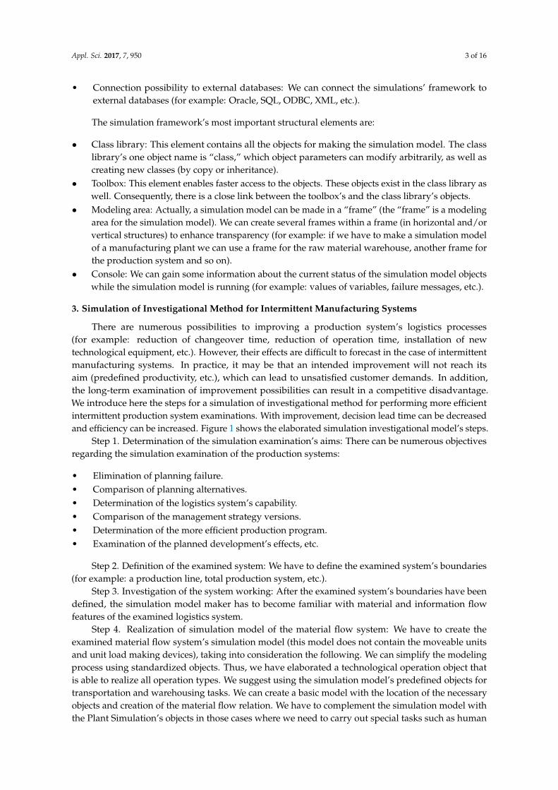
We have elaborated a simulation object (Figure 2) for the standardized modeling of all the technological operations. This allows for simpler and more standardized object control. If we are required to use a number of technological operation objects, in the interest of transparency we can use the frame object (a frame object can contain one or more technological objects).

Figure 2. Technological objects class.

Introduction of the elements of the technological objects class (Figure 2):

• Objects 1, 2: Input buffer object. • Object 3: Assembly tasks modeling object. • Object 4: Disassembly tasks modeling object. • Object 5: Parallel tasks modeling object.

Figure 1. Steps of the simulation investigation method of intermittent manufacturing systems.

(1). Technological objects class: We can distinguish four types of technological operations in anintermittent production system:

• Single operation: This technological workplace makes an operation on one product in a workcycle (for example: screw driving, turning, drilling, etc.).

• Parallel operation: This technological workplace makes an operation on several products ina work cycle (for example: heat treatment, painting, etc.).

• Assembly operation: This technological workplace makes one product out of several products ina work cycle.

• Disassembly operation: This technological workplace makes several products from one productin a work cycle.

We have elaborated a simulation object (Figure 2) for the standardized modeling of all thetechnological operations. This allows for simpler and more standardized object control. If we arerequired to use a number of technological operation objects, in the interest of transparency we can usethe frame object (a frame object can contain one or more technological objects).

Appl. Sci. 2017, 7, 950 4 of 17

Figure 1. Steps of the simulation investigation method of intermittent manufacturing systems.

(1). Technological objects class: We can distinguish four types of technological operations in an intermittent production system:

• Single operation: This technological workplace makes an operation on one product in a work cycle (for example: screw driving, turning, drilling, etc.).

• Parallel operation: This technological workplace makes an operation on several products in a work cycle (for example: heat treatment, painting, etc.).

• Assembly operation: This technological workplace makes one product out of several products in a work cycle.

• Disassembly operation: This technological workplace makes several products from one product in a work cycle.

We have elaborated a simulation object (Figure 2) for the standardized modeling of all the technological operations. This allows for simpler and more standardized object control. If we are required to use a number of technological operation objects, in the interest of transparency we can use the frame object (a frame object can contain one or more technological objects).

Figure 2. Technological objects class.

Introduction of the elements of the technological objects class (Figure 2):

• Objects 1, 2: Input buffer object. • Object 3: Assembly tasks modeling object. • Object 4: Disassembly tasks modeling object. • Object 5: Parallel tasks modeling object.

Figure 2. Technological objects class.

Introduction of the elements of the technological objects class (Figure 2):

• Objects 1, 2: Input buffer object.

Appl. Sci. 2017, 7, 950 5 of 16

• Object 3: Assembly tasks modeling object.• Object 4: Disassembly tasks modeling object.• Object 5: Parallel tasks modeling object.• Object 6: Output buffer. The finished products will go to the next operation in direct mode

(the product will be transmitted to the next workplace) or indirect mode (the unit load will betransmitted to the next workplace). The transmission will take place on the basis of the datatable’s data for the technological operation (see Step 6).

• Object 7: This object enables the placement of the unit load formation device (the productappearing on Object 6 will be loaded on Object 7’s unit load formation device in the case ofindirect transmission).

Table 1 presents the objects applied in technological operations (the control of the technologicalobject’s operation will be realized on the basis of the technological object’s data table; see Step 6).

Table 1. Applied objects in the case of technological operations.

Operation Type TransmissionMode Obj. 1 Obj. 2 Obj. 3 Obj. 4 Obj. 5 Obj. 6 Obj. 7

Simple Operation Direct X X X XIndirect X X X X X

Parallel Operation Direct X X X XIndirect X X X X X

Assembly Operation Direct X X X X XIndirect X X X X X X

Disassembly Operation Direct X X X XIndirect X X X X X

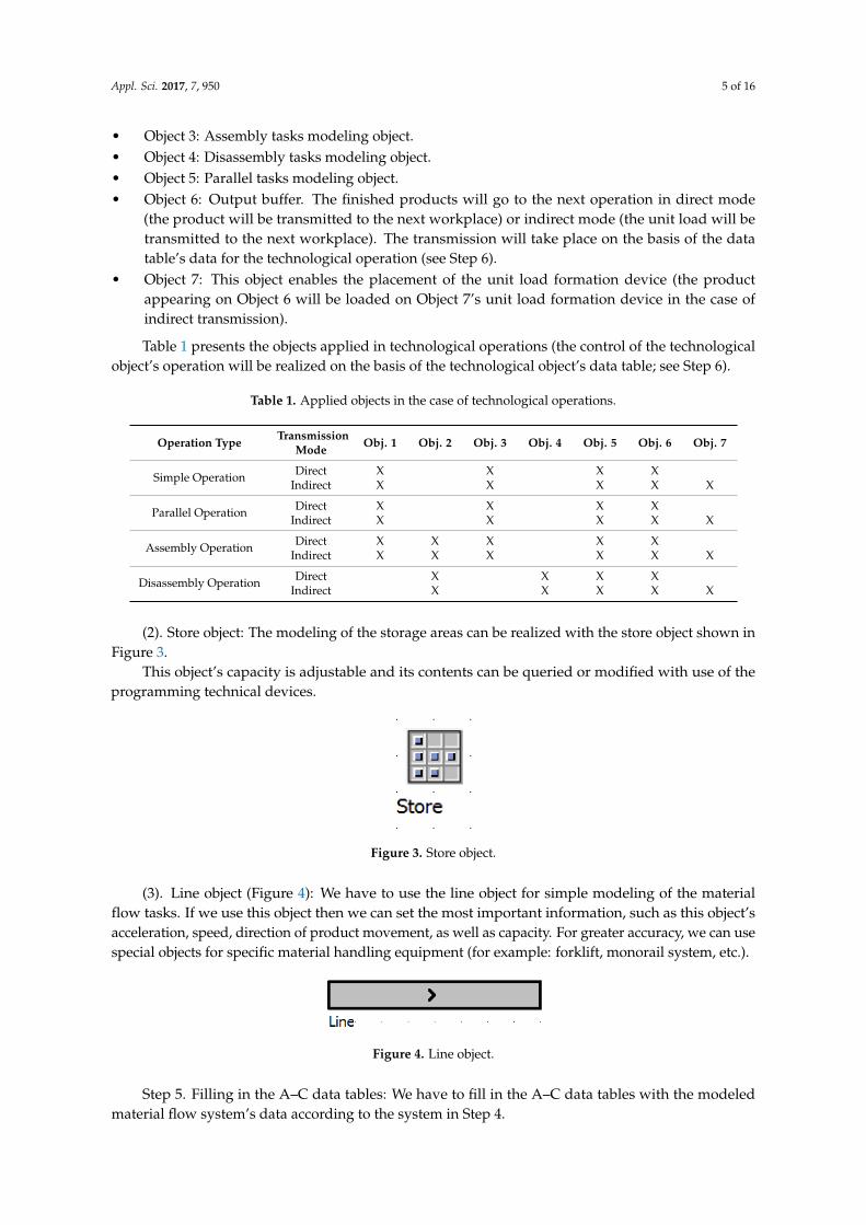
(2). Store object: The modeling of the storage areas can be realized with the store object shown inFigure 3.

This object’s capacity is adjustable and its contents can be queried or modified with use of theprogramming technical devices.

Appl. Sci. 2017, 7, 950 5 of 17

• Object 6: Output buffer. The finished products will go to the next operation in direct mode (the product will be transmitted to the next workplace) or indirect mode (the unit load will be transmitted to the next workplace). The transmission will take place on the basis of the data table’s data for the technological operation (see Step 6).

• Object 7: This object enables the placement of the unit load formation device (the product appearing on Object 6 will be loaded on Object 7’s unit load formation device in the case of indirect transmission).

Table 1 presents the objects applied in technological operations (the control of the technological object’s operation will be realized on the basis of the technological object’s data table; see Step 6).

Table 1. Applied objects in the case of technological operations.

Operation Type Transmission Mode Obj. 1 Obj. 2 Obj. 3 Obj. 4 Obj. 5 Obj. 6 Obj. 7

Simple Operation Direct X X X X

Indirect X X X X X

Parallel Operation Direct X X X X

Indirect X X X X X

Assembly Operation Direct X X X X X

Indirect X X X X X X

Disassembly Operation Direct X X X X

Indirect X X X X X

(2). Store object: The modeling of the storage areas can be realized with the store object shown in Figure 3.

This object’s capacity is adjustable and its contents can be queried or modified with use of the programming technical devices.

Figure 3. Store object.

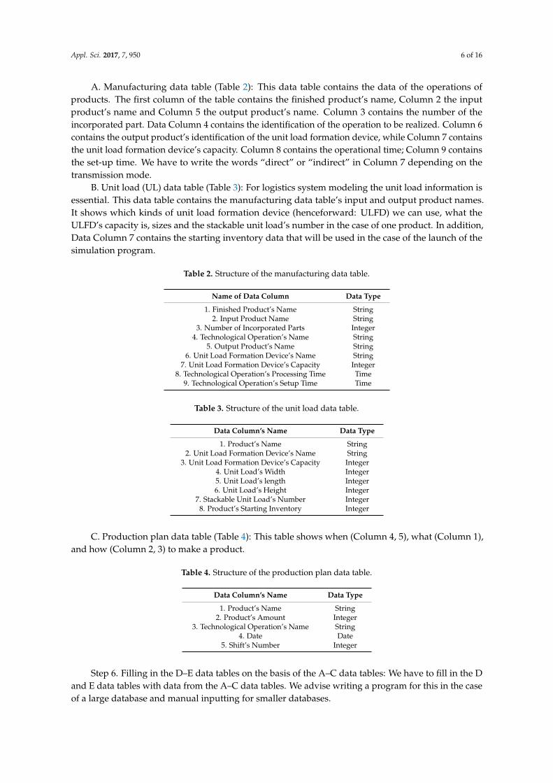
(3). Line object (Figure 4): We have to use the line object for simple modeling of the material flow tasks. If we use this object then we can set the most important information, such as this object’s acceleration, speed, direction of product movement, as well as capacity. For greater accuracy, we can use special objects for specific material handling equipment (for example: forklift, monorail system, etc.).

Figure 4. Line object.

Step 5. Filling in the A–C data tables: We have to fill in the A–C data tables with the modeled material flow system’s data according to the system in Step 4.

A. Manufacturing data table (Table 2): This data table contains the data of the operations of products. The first column of the table contains the finished product’s name, Column 2 the input product’s name and Column 5 the output product’s name. Column 3 contains the number of the incorporated part. Data Column 4 contains the identification of the operation to be realized. Column 6 contains the output product’s identification of the unit load formation device, while Column 7

Figure 3. Store object.

(3). Line object (Figure 4): We have to use the line object for simple modeling of the materialflow tasks. If we use this object then we can set the most important information, such as this object’sacceleration, speed, direction of product movement, as well as capacity. For greater accuracy, we can usespecial objects for specific material handling equipment (for example: forklift, monorail system, etc.).

Appl. Sci. 2017, 7, 950 5 of 17

• Object 6: Output buffer. The finished products will go to the next operation in direct mode (the product will be transmitted to the next workplace) or indirect mode (the unit load will be transmitted to the next workplace). The transmission will take place on the basis of the data table’s data for the technological operation (see Step 6).

• Object 7: This object enables the placement of the unit load formation device (the product appearing on Object 6 will be loaded on Object 7’s unit load formation device in the case of indirect transmission).

Table 1 presents the objects applied in technological operations (the control of the technological object’s operation will be realized on the basis of the technological object’s data table; see Step 6).

Table 1. Applied objects in the case of technological operations.

Operation Type Transmission Mode Obj. 1 Obj. 2 Obj. 3 Obj. 4 Obj. 5 Obj. 6 Obj. 7

Simple Operation Direct X X X X

Indirect X X X X X

Parallel Operation Direct X X X X

Indirect X X X X X

Assembly Operation Direct X X X X X

Indirect X X X X X X

Disassembly Operation Direct X X X X

Indirect X X X X X

(2). Store object: The modeling of the storage areas can be realized with the store object shown in Figure 3.

This object’s capacity is adjustable and its contents can be queried or modified with use of the programming technical devices.

Figure 3. Store object.

(3). Line object (Figure 4): We have to use the line object for simple modeling of the material flow tasks. If we use this object then we can set the most important information, such as this object’s acceleration, speed, direction of product movement, as well as capacity. For greater accuracy, we can use special objects for specific material handling equipment (for example: forklift, monorail system, etc.).

Figure 4. Line object.

Step 5. Filling in the A–C data tables: We have to fill in the A–C data tables with the modeled material flow system’s data according to the system in Step 4.

A. Manufacturing data table (Table 2): This data table contains the data of the operations of products. The first column of the table contains the finished product’s name, Column 2 the input product’s name and Column 5 the output product’s name. Column 3 contains the number of the incorporated part. Data Column 4 contains the identification of the operation to be realized. Column 6 contains the output product’s identification of the unit load formation device, while Column 7

Figure 4. Line object.

Step 5. Filling in the A–C data tables: We have to fill in the A–C data tables with the modeledmaterial flow system’s data according to the system in Step 4.

Appl. Sci. 2017, 7, 950 6 of 16

A. Manufacturing data table (Table 2): This data table contains the data of the operations ofproducts. The first column of the table contains the finished product’s name, Column 2 the inputproduct’s name and Column 5 the output product’s name. Column 3 contains the number of theincorporated part. Data Column 4 contains the identification of the operation to be realized. Column 6contains the output product’s identification of the unit load formation device, while Column 7 containsthe unit load formation device’s capacity. Column 8 contains the operational time; Column 9 containsthe set-up time. We have to write the words “direct” or “indirect” in Column 7 depending on thetransmission mode.

B. Unit load (UL) data table (Table 3): For logistics system modeling the unit load information isessential. This data table contains the manufacturing data table’s input and output product names.It shows which kinds of unit load formation device (henceforward: ULFD) we can use, what theULFD’s capacity is, sizes and the stackable unit load’s number in the case of one product. In addition,Data Column 7 contains the starting inventory data that will be used in the case of the launch of thesimulation program.

Table 2. Structure of the manufacturing data table.

Name of Data Column Data Type

1. Finished Product’s Name String2. Input Product Name String

3. Number of Incorporated Parts Integer4. Technological Operation’s Name String

5. Output Product’s Name String6. Unit Load Formation Device’s Name String

7. Unit Load Formation Device’s Capacity Integer8. Technological Operation’s Processing Time Time

9. Technological Operation’s Setup Time Time

Table 3. Structure of the unit load data table.

Data Column’s Name Data Type

1. Product’s Name String2. Unit Load Formation Device’s Name String

3. Unit Load Formation Device’s Capacity Integer4. Unit Load’s Width Integer5. Unit Load’s length Integer6. Unit Load’s Height Integer

7. Stackable Unit Load’s Number Integer8. Product’s Starting Inventory Integer

C. Production plan data table (Table 4): This table shows when (Column 4, 5), what (Column 1),and how (Column 2, 3) to make a product.

Table 4. Structure of the production plan data table.

Data Column’s Name Data Type

1. Product’s Name String2. Product’s Amount Integer

3. Technological Operation’s Name String4. Date Date

5. Shift’s Number Integer

Step 6. Filling in the D–E data tables on the basis of the A–C data tables: We have to fill in the Dand E data tables with data from the A–C data tables. We advise writing a program for this in the caseof a large database and manual inputting for smaller databases.

Appl. Sci. 2017, 7, 950 7 of 16

D. Control data table (Table 5): The control data table shows what kinds of operations the partsneed to go through in order to make the finished product. The control data table has to be created on thebasis of the manufacturing data table’s data (the product’s manufacturing’s process can be built on thebasis of the manufacturing data table’s data Column 1–5). Modification of the product’s manufacturingprocess is done modifying of the control data table’s data. The control data table’s contains a finishedproduct’s manufacturing process where the first column’s product names are the same. If a productgoes through an operation then its name will change. Consequently the previous operation’s outputproduct (Data Column 3) will be the following operation’s input product (Data Column 2). The controldata table shows how output product (Column data 3) proceeds from the input product (Columndata 2) through the operations (Data Column 4 and so on). We have to mark those cells’ value with“1” where the given product’s (line) assigned operation (Column) will be realized. A chained list willbe created regarding the finished products where the final step’s result will be the finished products.The control data table contains all of the finished products’ material flow.

Table 5. Structure of the control data table.

Data Column’s Name Data Type

1. Finished product’s Name String2. Input Product’s Name String

3. Output Product’s Name String4. Technological Operation 1 String5. Technological Operation 2 String

. . . . . . String

E. Technological operation data table (Table 6): This data table will be filled on the basis of theproduction plan, control, and the manufacturing data tables. This data table is created in the caseof every technological operation, and tables contain the activities to be realized. The data table willshow which input product (Data Column 2) do we need to work on, what the size of the series is(Data Column 3), what the material catering’s starting station is (Data Column 4), what the workedproduct’s ULFD is (Data Column 6), and the ULFD capacity (Data Column 7). In addition, this datatable contains the product processing’s operation time (Data Column 8) and set up time (Data Column9). Programming is suggested for bigger databases.

Step 7. Definition and adaptation of the evaluation indicators: We have to define the indicatorsto be examined while taking into consideration the investigational objectives and then adjust theindicators in the simulation model (for example: maximum stock level, operating costs, etc.).

Most simulation framework systems are able to visualize the examined indicator’s data(for example: frequency function, distribution function, diagrams), which contributes to moreefficient decision-making.

Table 6. Structure of the technological operation data table.

Data Column’s Name Data Type

1. Finished Product’s Name String2. Input Product’s Name String

3. Product’s Number Integer4. Source Object’s Name String

5. Output Product’s Name String6. ULFD’s Name String

7. ULFD’s Capacity Integer8. Technological Operation’s Processing Time Time

9. Technological Operation’s Setup Time Time

Step 8. Creation and running the simulation program: We have to run the simulation program inthe following way. The first step is creation of the movable units (products, ULFD) and starting stocks

Appl. Sci. 2017, 7, 950 8 of 16

on the basis of the unit load data table. Next the manufacturing processes’ control has to be realizedon the basis of the technological object data table (every object has such a data table). The data tables’instructions have to be performed line by line. The chosen indicator’s value has to be determined byrunning the simulation model.

Step 9. Evaluation of the determined results: We have to evaluate the determined indicators’values after the simulation has been run.

Step 10. Making the decision: After the evaluation, we have to make decisions about a newexamination (Step 5) or realization of the improvement (Step 11).

4. Possible Applications of a Decision-Making Simulation Method

Continuous changes of the product types and amounts to be produced based on customer needsresults in frequent re-planning of the logistics processes of intermittent production systems. The effectsof the alteration to be realized can be difficult to forecast because of the examined system’s complexity;consequently, it is necessary to reduce the decision risks by high precision determination of differentlogistics indicators. The value of the needed indicators can be determined by the elaborated simulationinvestigational method; thus, the improvement decision can be made with minimum risk. We examinea planned system’s working by application of the investigational method, where the decision’s resultcan be realization of the examined system or execution of a new examination with modified parametersbased on the values of the determined indicators. We have to execute the simulation examinationswhile obtaining the necessary data for the final decision. This can be a repetitive process. The elaboratedinvestigational method is suitable for the following cases:

(1). Decision support for determination of the storage capacity to be created: Precise determinationof the storage capacity needed for a system to be realized can cause significant difficulty because of thecomplexity of the processes. In such cases the necessary controls and alterations can be executed bythe elaborated simulation method.

Most important indicator:

- Maximum stock level: This is how to determine the maximum storage capacity need(s) regardingone or more storage systems. The maximum stock level of the storage system s can be calculatedas follows:

QMaxs = max

t∈ΘS

{qSo + qsbz − qskt

}, (1)

where ΘS is the date when stock movements were executed, qSo is the starting stock level,qsbt contains the stocked in amounts, qskt the stocked out product quantities regarding date t.

(2). Decision support for determination of the material handling equipment’s efficient utilization:The working strategy and efficiency of the material handling equipment can be difficult toevaluate before the realization of the examined system regarding the intermittent productionsystems, but the necessary controls and alterations can be executed by using elaborated simulationinvestigational method.

Most important indicators:

- Rate of the effective route length: This expresses what percentage of the material handlingequipment’s total traveled route length was executed without an unladen vehicle. The rate of theeffective route length in case of the material handling equipment m can be calculated as follows:

RUm = ∑

d∈ΘUm

(ld)/ ∑d∈Θm

(ld), (2)

where Θm is a set containing the identification of the traveled route sections for the materialhandling equipment m, ΘU

m includes the identification of the effective route sections, and ldindicates the length of the route section d according to Equation (2).

Appl. Sci. 2017, 7, 950 9 of 16

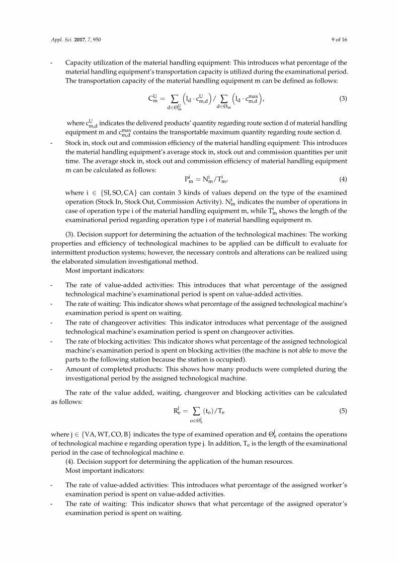
- Capacity utilization of the material handling equipment: This introduces what percentage of thematerial handling equipment’s transportation capacity is utilized during the examinational period.The transportation capacity of the material handling equipment m can be defined as follows:

CUm = ∑

d∈ΘUm

(ld · cU

m,d

)/ ∑

d∈Θm

(ld · cmax

m,d

), (3)

where cUm,d indicates the delivered products’ quantity regarding route section d of material handling

equipment m and cmaxm,d contains the transportable maximum quantity regarding route section d.

- Stock in, stock out and commission efficiency of the material handling equipment: This introducesthe material handling equipment’s average stock in, stock out and commission quantities per unittime. The average stock in, stock out and commission efficiency of material handling equipmentm can be calculated as follows:

Pim = Ni

m/Tim, (4)

where i ∈ {SI, SO, CA} can contain 3 kinds of values depend on the type of the examinedoperation (Stock In, Stock Out, Commission Activity). Ni

m indicates the number of operations incase of operation type i of the material handling equipment m, while Ti

m shows the length of theexaminational period regarding operation type i of material handling equipment m.

(3). Decision support for determining the actuation of the technological machines: The workingproperties and efficiency of technological machines to be applied can be difficult to evaluate forintermittent production systems; however, the necessary controls and alterations can be realized usingthe elaborated simulation investigational method.

Most important indicators:

- The rate of value-added activities: This introduces that what percentage of the assignedtechnological machine’s examinational period is spent on value-added activities.

- The rate of waiting: This indicator shows what percentage of the assigned technological machine’sexamination period is spent on waiting.

- The rate of changeover activities: This indicator introduces what percentage of the assignedtechnological machine’s examination period is spent on changeover activities.

- The rate of blocking activities: This indicator shows what percentage of the assigned technologicalmachine’s examination period is spent on blocking activities (the machine is not able to move theparts to the following station because the station is occupied).

- Amount of completed products: This shows how many products were completed during theinvestigational period by the assigned technological machine.

The rate of the value added, waiting, changeover and blocking activities can be calculatedas follows:

Rje = ∑

o∈Θje

(to)/Te (5)

where j ∈ {VA, WT, CO, B} indicates the type of examined operation and Θje contains the operations

of technological machine e regarding operation type j. In addition, Te is the length of the examinationalperiod in the case of technological machine e.

(4). Decision support for determining the application of the human resources.Most important indicators:

- The rate of value-added activities: This introduces what percentage of the assigned worker’sexamination period is spent on value-added activities.

- The rate of waiting: This indicator shows that what percentage of the assigned operator’sexamination period is spent on waiting.

Appl. Sci. 2017, 7, 950 10 of 16

- The rate of changeover activities: This indicator introduces the percentage of the assignedoperator’s examination period spent on changeover activities.

- The rate of blocking activities: This indicator shows the percentage of the assigned operator’sexamination period spent idle due to blocking activities (the person is not able to move the partsto the following station because of the station’s occupation).

- Amount of completed products: This shows the number of products completed during theinvestigational period by the assigned operator.

The rate of the value-added, waiting, changeover, and blocking activities can be calculatedas follows:

Rkh = ∑

o∈Θkh

(t0)/Th, (6)

where k ∈ {VA, WT, CO, B} indicates the type of examined operation and Θkh contains the operations of

the human resource h regarding the operation type k. In addition, Th is the length of the examinationalperiod in case of the human resource h.

In most cases, the above indicators give appropriate support for making an improved decision,although in some special examinations it may be necessary to examine other indicators as well e.g., if wehave to define the floor area for storage instead of storage capacity need). In addition, visualizing thedetermined indicator values with diagrams can provide relevant help to support decision-making.

5. Application of the Elaborated Simulation Investigational Method

In this section, we will introduce the elaborated investigational method through an imaginedassembly cell’s examination.

Steps of the examination:Step 1. Determination of the simulation examination’s aims: The main objective is the

determination of the inter-operational store’s floor area’s size. There can be necessary the realization ofthe examination in many cases, e.g., if the product structure to be produced or the production planwill change at a relevant complexity manufacturing system in the future [6].

Step 2. Definition of the examined system: the examined manufacturing cell contains 16 stagesoperations and seven stages of inter-operation storage. These objects will get the parts from themanufacturing plant and send the completed parts to the finished goods storage.

Step 3. Investigation of the system working: we defined the most important characteristics inorder to describe the working of the examined system (e.g., operational time, mode of the working,changeover time, applied unit load forming device, unit load forming device’s capacity, mode ofmaterials handling in case of every product). We want to create a complex manufacturing cell in orderto test the method.

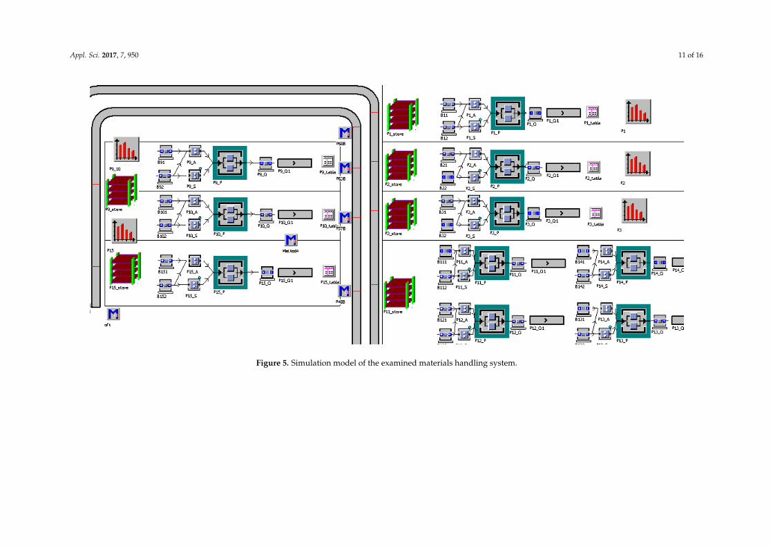
Step 4. Realization of simulation model of the material flow system: we placed the materialflow system’s objects on the basis of instructions in Section 3 (16 operations, seven stages of theinter-operational storage, traffic routes), as well as defining the material flow connections betweenthese objects (Figure 5). The inter-operational storage is realized on floor level with stacking.

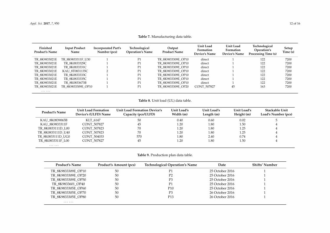
Step 5. Filling in the A–C data tables: Uploading the manufacturing data table (Table 7), unit loaddata table (Table 8), and the production plan data table (Table 9) with the investigational data. Step 5in Section 3 gives guidance for interpreting Tables 7–9.

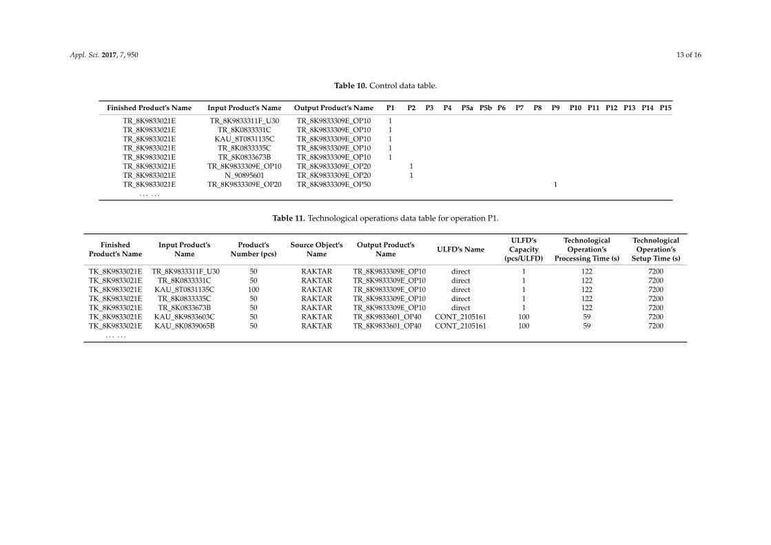
Step 6. Filling in Data tables D and E on the basis of data from A–C data tables: in this step thedata of the control data table (Table 10) is input from the manufacturing (A) and the production plan(C) data tables. In addition the production plan (C), manufacturing (A) and the control (D) data tables’data are input to the technological operation data table (Table 11). We have to fill out a data table foreach operation (16 operations). We can automate this upload (for large databases), or we can input itmanually (for small databases). Step 5 in Section 3 gives guidance for interpreting Tables 10 and 11.

Appl. Sci. 2017, 7, 950 11 of 16Appl. Sci. 2017, 7, x FOR PEER REVIEW 11 of 17

Figure 5. Simulation model of the examined materials handling system. Figure 5. Simulation model of the examined materials handling system.

Appl. Sci. 2017, 7, 950 12 of 16

Table 7. Manufacturing data table.

FinishedProduct’s Name

Input ProductName

Incorporated Part’sNumber (pcs)

TechnologicalOperation’s Name

OutputProduct Name

Unit LoadFormation

Device’s Name

Unit LoadFormation

Device’s Name

TechnologicalOperation’s

Processing Time (s)

SetupTime (s)

TR_8K9833021E TR_8K9833311F_U30 1 P1 TR_8K9833309E_OP10 direct 1 122 7200TR_8K9833021E TR_8K0833329C 1 P1 TR_8K9833309E_OP10 direct 1 122 7200TR_8K9833021E TR_8K0833331C 1 P1 TR_8K9833309E_OP10 direct 1 122 7200TR_8K9833021E KAU_8T0831135C 2 P1 TR_8K9833309E_OP10 direct 1 122 7200TR_8K9833021E TR_8K0833333C 1 P1 TR_8K9833309E_OP10 direct 1 122 7200TR_8K9833021E TR_8K0833335C 1 P1 TR_8K9833309E_OP10 direct 1 122 7200TR_8K9833021E TR_8K0833673B 1 P1 TR_8K9833309E_OP10 direct 1 122 7200TR_8K9833021E TR_8K9833309E_OP10 1 P1 TR_8K9833309E_OP20 CONT_507827 45 163 7200

. . . . . .

Table 8. Unit load (UL) data table.

Product’s Name Unit Load FormationDevice’s (ULFD) Name

Unit Load Formation Device’sCapacity (pcs/ULFD)

Unit Load’sWidth (m)

Unit Load’sLength (m)

Unit Load’sHeight (m)

Stackable UnitLoad’s Number (pcs)

KAU_8K0839065B KLT_6147 50 0.40 0.60 0.02 5KAU_8K9833311F CONT_507827 45 1.20 1.80 1.50 4

TR_8K0833111D_L00 CONT_507823 70 1.20 1.80 1.25 4TR_8K0833111D_U40 CONT_507823 70 1.20 1.80 1.25 4TR_8K0833111D_UG0 CONT_504033 570 1.80 2.40 0.74 4TR_8K0833311F_L00 CONT_507827 45 1.20 1.80 1.50 4

. . . . . .

Table 9. Production plan data table.

Product’s Name Product’s Amount (pcs) Technological Operation’s Name Date Shifts’ Number

TR_8K9833309E_OP10 50 P1 25 October 2016 1TR_8K9833309E_OP20 50 P2 25 October 2016 1TR_8K9833309E_OP50 50 P3 25 October 2016 1TR_8K9833601_OP40 50 P1 25 October 2016 1

TR_8K9833305E_OP60 50 P10 25 October 2016 1TR_8K9833305E_OP70 50 P3 26 October 2016 1TR_8K9833305E_OP80 50 P13 26 October 2016 1

. . . . . .

Appl. Sci. 2017, 7, 950 13 of 16

Table 10. Control data table.

Finished Product’s Name Input Product’s Name Output Product’s Name P1 P2 P3 P4 P5a P5b P6 P7 P8 P9 P10 P11 P12 P13 P14 P15

TR_8K9833021E TR_8K9833311F_U30 TR_8K9833309E_OP10 1TR_8K9833021E TR_8K0833331C TR_8K9833309E_OP10 1TR_8K9833021E KAU_8T0831135C TR_8K9833309E_OP10 1TR_8K9833021E TR_8K0833335C TR_8K9833309E_OP10 1TR_8K9833021E TR_8K0833673B TR_8K9833309E_OP10 1TR_8K9833021E TR_8K9833309E_OP10 TR_8K9833309E_OP20 1TR_8K9833021E N_90895601 TR_8K9833309E_OP20 1TR_8K9833021E TR_8K9833309E_OP20 TR_8K9833309E_OP50 1

. . . . . .

Table 11. Technological operations data table for operation P1.

FinishedProduct’s Name

Input Product’sName

Product’sNumber (pcs)

Source Object’sName

Output Product’sName ULFD’s Name

ULFD’sCapacity

(pcs/ULFD)

TechnologicalOperation’s

Processing Time (s)

TechnologicalOperation’s

Setup Time (s)

TK_8K9833021E TR_8K9833311F_U30 50 RAKTAR TR_8K9833309E_OP10 direct 1 122 7200TK_8K9833021E TR_8K0833331C 50 RAKTAR TR_8K9833309E_OP10 direct 1 122 7200TK_8K9833021E KAU_8T0831135C 100 RAKTAR TR_8K9833309E_OP10 direct 1 122 7200TK_8K9833021E TR_8K0833335C 50 RAKTAR TR_8K9833309E_OP10 direct 1 122 7200TK_8K9833021E TR_8K0833673B 50 RAKTAR TR_8K9833309E_OP10 direct 1 122 7200TK_8K9833021E KAU_8K9833603C 50 RAKTAR TR_8K9833601_OP40 CONT_2105161 100 59 7200TK_8K9833021E KAU_8K0839065B 50 RAKTAR TR_8K9833601_OP40 CONT_2105161 100 59 7200

. . . . . .

Appl. Sci. 2017, 7, 950 14 of 16

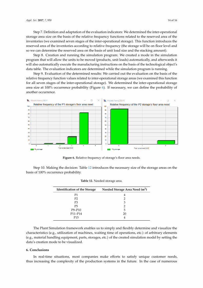
Step 7. Definition and adaptation of the evaluation indicators: We determined the inter-operationalstorage area size on the basis of the relative frequency functions related to the reserved area of theinventories (we examined seven stages of the inter-operational storage). This function introduces thereserved area of the inventories according to relative frequency (the storage will be on floor level andso we can determine the reserved area on the basis of unit load size and the stacking amount).

Step 8. Creation and running the simulation program: We created a mode in the simulationprogram that will allow the units to be moved (products, unit loads) automatically, and afterwards itwill also automatically execute the manufacturing instructions on the basis of the technological object’sdata table. The evaluation indicators are determined while the simulation program is running.

Step 9. Evaluation of the determined results: We carried out the evaluation on the basis of therelative frequency function values related to inter-operational storage areas (we examined this functionfor all seven stages of the inter-operational storage). We determined the inter-operational storagearea size at 100% occurrence probability (Figure 6). If necessary, we can define the probability ofanother occurrence.

Appl. Sci. 2017, 7, x FOR PEER REVIEW 14 of 17

Step 7. Definition and adaptation of the evaluation indicators: We determined the inter-operational storage area size on the basis of the relative frequency functions related to the reserved area of the inventories (we examined seven stages of the inter-operational storage). This function introduces the reserved area of the inventories according to relative frequency (the storage will be on floor level and so we can determine the reserved area on the basis of unit load size and the stacking amount).

Step 8. Creation and running the simulation program: We created a mode in the simulation program that will allow the units to be moved (products, unit loads) automatically, and afterwards it will also automatically execute the manufacturing instructions on the basis of the technological object’s data table. The evaluation indicators are determined while the simulation program is running.

Step 9. Evaluation of the determined results: We carried out the evaluation on the basis of the relative frequency function values related to inter-operational storage areas (we examined this function for all seven stages of the inter-operational storage). We determined the inter-operational storage area size at 100% occurrence probability (Figure 6). If necessary, we can define the probability of another occurrence.

Figure 6. Relative frequency of storage’s floor area needs.

Step 10. Making the decision: Table 12 introduces the necessary size of the storage areas on the basis of 100% occurrence probability.

Table 12. Needed storage area.

Identification of the Storage Needed Storage Area Need (m2) P1 4 P2 2 P3 3 P5 2

P9–P10 5 P11–P14 20

P15 4

The Plant Simulation framework enables us to simply and flexibly determine and visualize the characteristics (e.g., utilization of machines, waiting time of operations, etc.) of arbitrary elements (e.g., material handling equipment, parts, storages, etc.) of the created simulation model by setting the data’s creation mode to be visualized.

Figure 6. Relative frequency of storage’s floor area needs.

Step 10. Making the decision: Table 12 introduces the necessary size of the storage areas on thebasis of 100% occurrence probability.

Table 12. Needed storage area.

Identification of the Storage Needed Storage Area Need (m2)

P1 4P2 2P3 3P5 2

P9–P10 5P11–P14 20

P15 4

The Plant Simulation framework enables us to simply and flexibly determine and visualize thecharacteristics (e.g., utilization of machines, waiting time of operations, etc.) of arbitrary elements(e.g., material handling equipment, parts, storages, etc.) of the created simulation model by setting thedata’s creation mode to be visualized.

6. Conclusions

In real-time situations, most companies make efforts to satisfy unique customer needs,thus increasing the complexity of the production systems in the future. In the case of numerous

Appl. Sci. 2017, 7, 950 15 of 16

complex logistics systems, application of a decision support simulation method is required for makingappropriate improvement decisions.

Such a method examines production systems where the parameters of the logistics processes ofproduct families can significantly differ from each other (in operation times, changeover times, batch sizes,types of the unit load forming devices, etc.) and where material flow nodes and backflows occur.

After a review of the literature, it was found that simulation examinations have tended to berelated to production processes of one product family and/or contained several simplifications; I havenot found any other elaborated simulation investigational method that enables the realization ofsimulation examination regarding every type of intermittent production system. In order to eliminatethis gap, in this paper I have elaborated and introduced a decision support simulation method basedon my practical experience. Realization of the simulation investigational model can take less timethan in earlier methods (the modeling steps are clear and simple to implement) and we can alsoexamine every complex intermittent production systems (production systems in the automotive orelectronic industries, etc.) using the elaborated investigational method. The method focuses on theindicators of present and the future intermittent production systems that are most important for makinga correct improvement decision or for avoiding possible improvement failures (e.g., low productivity,small storage capacity, etc.), without discussing the optimization possibilities of the intermittentproduction system.

Future aims are to work out data structures that enable the automatic creation of the investigationmodel. If this can be realized, the investigation’s lead time will be reduced. Elaboration and adaptationof several optimization algorithms is another potential research area (e.g., route planning, volume oftime schedule of production, etc.).

Acknowledgments: The described research was carried out as part of the EFOP-3.6.1-16-00011 “Younger andRenewing University—Innovative Knowledge City—institutional development of the University of Miskolcaiming at intelligent specialization” project implemented in the framework of the Szechenyi 2020 program.The realization of this project is supported by the European Union, co-financed by the European Social Fund.

Conflicts of Interest: The authors declare no conflict of interest.

References

1. Womack, J.P.; Jones, D.T. Lean Thinking; Simon & Schuster Inc.: Delran, NJ, USA, 2008.2. Rother, M.; Shook, J. Learning to See: Value Stream Mapping to Add Value and Eliminate Muda; Lean Enterprise

Institute: Cambridge, MA, USA, 2003.3. Cselényi, J.; Illés, B. Planning and Controlling of Material Flow Systems; Textbook; Miskolci Egyetemi Kiadó:

Miskolc, Hungary, 2006.4. Tyagi, S.; Choudhary, A.; Cai, X.; Yang, K. Value stream mapping to reduce the lead-time of a product

development process. Int. J. Prod. Econ. 2015, 160, 202–212. [CrossRef]5. Košt’ál, P.; Velíšek, K. Flexible Manufacturing System. World Acad. Sci. Eng. Technol. Int. J. Mech. Aerosp. Ind.

Mechatron. Manuf. Eng. 2011, 5, 917–921.6. Tamás, P. Application of value stream mapping at flexible manufacturing systems. Key Eng. Mater. 2016, 686,

168–173. [CrossRef]7. Bratley, P.; Fox, B.L.; Schrage, L.E. A Guide to Simulation, 2nd ed.; Springer: New York, NY, USA, 1987;

ISBN 978-1-4612-6457-6.8. Tako, A.A.; Robinson, S. The application of discrete event simulation and system dynamics in the logistics

and supply chain context. Decis. Support Syst. 2012, 52, 802–815. [CrossRef]9. Rodic, A.; Mester, G. The Modeling and Simulation of an Autonomous QuadRotor Microcopter in a Virtual

Outdoor Scenario. Acta Polytech. Hung. 2011, 8, 107–122.10. Gubán, M.; Gubán, Á. Production scheduling with genetic algorithm. Adv. Logist. Syst. Theory Pract. 2012, 6,

33–44.11. Sadiku, M.; Tofighi, M. A tutorial on simulation of queueing models. Int. J. Electr. Eng. Educ. 1999, 36,

102–120. [CrossRef]

Appl. Sci. 2017, 7, 950 16 of 16

12. Erdélyi, F.; Tóth, T.; Kulcsár, G.Y.; Mileff, P.; Hornyák, O.; Nehéz, K.; Körei, A. New Models and Methods forIncreasing the Efficiency of Customized Mass Production. J. Mach. Manuf. 2009, 49, 11–17.

13. Despotovic-Zrakic, D.; Barac, D.; Bogdanovic, Z.; Jovanic, B.; Radenkovic, B. Software Environment forLearning Continuous System Simulation. Acta Polytech. Hung. 2014, 11, 107–122. [CrossRef]

14. Solding, P.; Gullander, P. Concepts for simulation based value stream mapping. In Proceedings of the 2009Winter Simulation Conference, Austin, TX, USA, 13–16 December 2009; pp. 2231–2237.

15. D’Uffizi, A.; Simonetti, M.; Stecca, G.; Confessore, G. A Simulation Study of Logistics for Disaster ReliefOperations. Procedia CIRP 2015, 33, 157–162. [CrossRef]

16. Leriche, D.; Oudani, M.; Cabani, A.; Hoblos, G.; Mouzna, J.; Boukachour, J.; El Hilali Alaoui, A. Simulatingnew logistics system of Le Havre Port. IFAC-PapersOnLine 2015, 48, 418–423. [CrossRef]

17. Sui, X.; Han, G.; Chen, F. Numerical simulation on air distribution of a tennis hall winter and evaluation onindoor thermal environment. Eng. Rev. 2014, 34, 109–118.

18. Izadi, M.; Razavi, F. Loss reduction in a distribution system by considering interest rate. Eng. Rev. 2015, 35,179–191.

19. Rybicka, J.; Tiwari, A. Testing a flexible manufacturing system facility production capacity through discreteevent simulation: Automotive case study. World Acad. Sci. Eng. Technol. Int. J. Mech. Aerosp. Ind. Mechatron.Manuf. Eng. 2016, 10, 712–716.

20. Jilcha, K.; Berhan, E.; Sherif, H. Workers and Machine Performance Modeling in Manufacturing SystemUsing Arena Simulation. Comput. Sci. Syst. Biol. 2015. [CrossRef]

21. Arkadiusz, G.; Antoni, S. Simulation Based Analysis of Reconfigurable Manufacturing System Configurations.Appl. Mech. Mater. 2016, 844, 50–59.

22. Renna, P. Allocation improvement policies to reduce process time based on workload evaluation in job shopmanufacturing systems. Int. J. Ind. Eng. Comput. 2017, 8, 373–384. [CrossRef]

23. Kitazawa, M.; Takahashi, S.; Takahashi, T.; Ternao, T. Improving a Cellular Manufacturing System throughReal Time-Simulation and -Measurement. In Proceedings of the 2016 IEEE 40th Annual Computer Softwareand Applications Conference (COMPSAC), Atlanta, GA, USA, 10–14 June 2016. [CrossRef]

24. Song, B.; Hutabarat, W.; Tiwari, A. Integrating optimization of simulation for flexible manufacturingsystem. In Proceedings of the 14th International Conference on Manufacturing Research, Loughborough,UK, 6–8 September 2016. [CrossRef]

25. Hachicha, W.; Triki, H. Manufacturing System Design Based on Axiomatic Design: Case of Assembly Line.J. Ind. Eng. Manag. 2017. [CrossRef]

26. Martinez, J.; Muro, P.; Silva, M. Modelling, Validation and Software Implementation of Production SystemsUsing High-Level Petri Nets. In Proceedings of the IEEE Conference on Robotics and Automation, Raleigh,NC, USA, 31 March–3 April 1987; pp. 307–314.

27. Hillion, H.P. Timed Petri Nets and Application to Multi-Stage Production Systems; Advances in Petri Nets;Springer: New York, NY, USA, 1989.

28. Abdul-Hussin, M.H. Elementary Siphons of Petri Nets and Deadlock Control in FMS. J. Comput. Commun.2015, 1–12. [CrossRef]

29. Li, Z.W.; Zhou, M.C. Elementary siphons of Petri nets and their application to deadlock prevention in flexiblemanufacturing systems. IEEE Trans. Syst. Man Cybern. A 2004, 34, 38–51. [CrossRef]

30. Tamás, P.; Illés, B. Simulation examination of logistics systems in the automotive industry. J. Prod. Eng. 2015,18, 69–72.

31. Tamás, P.; Illés, B.; Tollár, S. Simulation of a flexible manufacturing system. Adv. Logist. Syst. Theory Pract.2012, 6, 25–32.

32. Dobos, P.; Illés, B.; Tamás, P. Conception for selection of adequate warehousing material handling strategy.Adv. Logist. Syst. Theory Pract. 2015, 9, 53–60.

33. Available online: https://www.plm.automation.siemens.com/en/products/tecnomatix/manufacturing-simulation/material-flow/plant-simulation.shtml (accessed on 10 August 2017).

© 2017 by the author. Licensee MDPI, Basel, Switzerland. This article is an open accessarticle distributed under the terms and conditions of the Creative Commons Attribution(CC BY) license (http://creativecommons.org/licenses/by/4.0/).