Embed Size (px)
Citation preview

DECISION MODELING WITH DECISION MODELING WITH MICROSOFT EXCELMICROSOFT EXCEL
Copyright 2001Prentice Hall
Chapter 5Chapter 5
LINEAR OPTIMIZATION:LINEAR OPTIMIZATION:APPLICATIONSAPPLICATIONS
Part 1Part 1
Chapter 5Chapter 5
LINEAR OPTIMIZATION:LINEAR OPTIMIZATION:APPLICATIONSAPPLICATIONS
Part 1Part 1

IntroductionIntroductionSeveral specific models (which can be used as templates for real-life problems) will be examined in this chapter. These models include:
TRANSPORTATION MODELTRANSPORTATION MODEL
ASSIGNMENT MODELASSIGNMENT MODEL
Management must determine how to send products from various sources to various destinations in order to satisfy requirements at the lowest possible cost.
Allows management to investigate allocating fixed-sized resources to determine the optimal assignment of salespeople to districts, jobs to machines, tasks to computers …

DYNAMIC (MULTIPERIOD) MODELDYNAMIC (MULTIPERIOD) MODEL
MEDIA SELECTION MODELMEDIA SELECTION MODEL
NETWORK MODELSNETWORK MODELS
This model is concerned with designing an effective advertising campaign.
These are models in which coordinated decision making must occur over more than one time period.
FINANCIAL AND PRODUCTION PLANNINGFINANCIAL AND PRODUCTION PLANNING These business models illustrate the joint optimization of both production and financial resources.
These models involve the movement or assignment of physical entities (e.g., money).
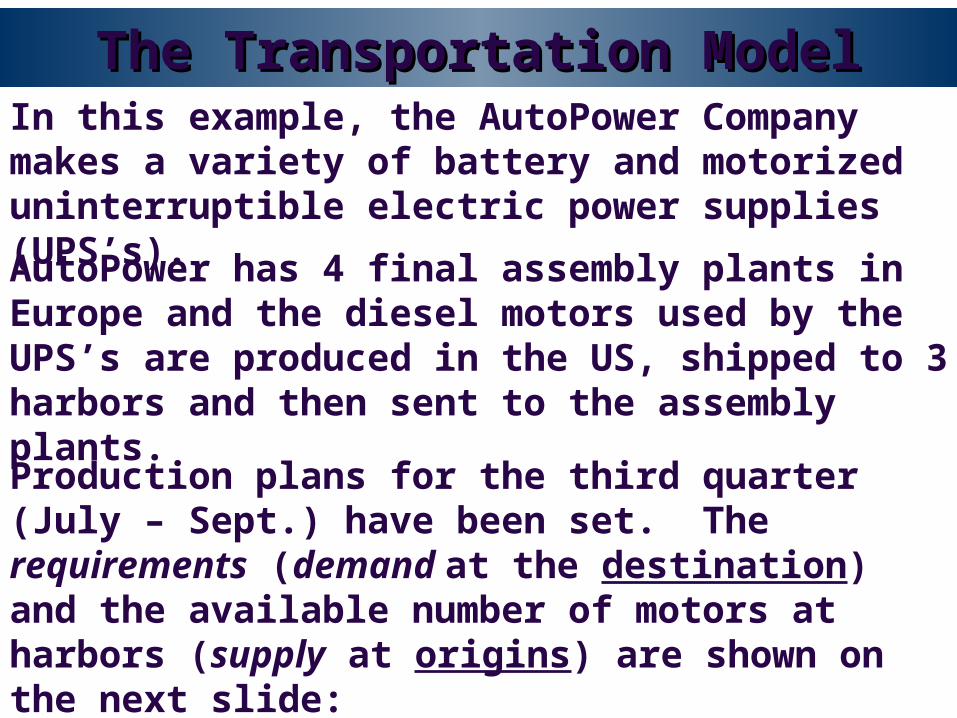
The Transportation ModelThe Transportation ModelIn this example, the AutoPower Company makes a variety of battery and motorized uninterruptible electric power supplies (UPS’s).
AutoPower has 4 final assembly plants in Europe and the diesel motors used by the UPS’s are produced in the US, shipped to 3 harbors and then sent to the assembly plants.
Production plans for the third quarter (July – Sept.) have been set. The requirements (demand at the destination) and the available number of motors at harbors (supply at origins) are shown on the next slide:
DemandDemand
SupplySupply
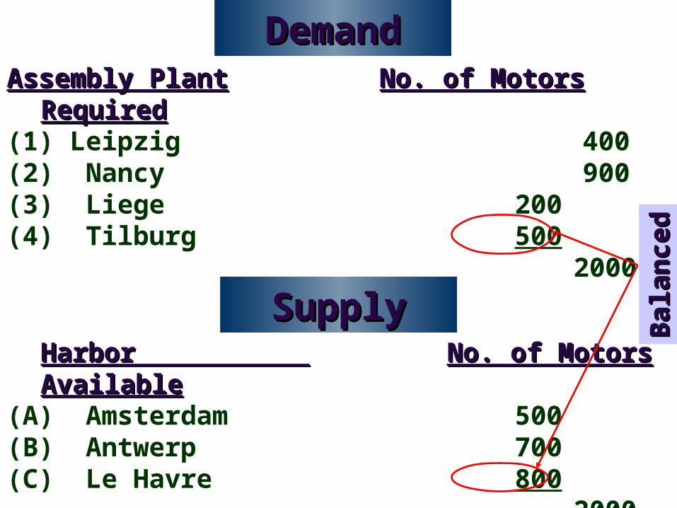
Assembly PlantAssembly Plant No. of Motors RequiredNo. of Motors Required(1) Leipzig 400(2) Nancy 900(3) Liege 200(4) Tilburg 500
2000
Harbor Harbor No. of Motors No. of Motors AvailableAvailable
(A) Amsterdam 500(B) Antwerp 700(C) Le Havre 800
2000
Bal
ance
dB
alan
ced

Graphical presentation of
Le Havre (Le Havre (CC))
800
Antwerp (Antwerp (BB))
700
Amsterdam (Amsterdam (AA))500
SupplySupply
Liege (3)Liege (3)
200
Tilburg (4)Tilburg (4)500
Leipzig (1)Leipzig (1)400
Nancy (2)Nancy (2)900
and Demand:Demand:

The Transportation ModelThe Transportation Model
AutoPower must decide how many motors to send from each harbor (supply) to each plant (demand).
The cost ($, on a per motor basis) of shipping is given below.
TO DESTINATIONTO DESTINATION Leipzig Nancy Liege Leipzig Nancy Liege
TilburgTilburgFROM ORIGINFROM ORIGIN (1) (2) (3) (4)(1) (2) (3) (4)
(A) Amsterdam(A) Amsterdam 120 130 41 59.50
(B) Antwerp(B) Antwerp 61 40 100 110
(C) Le Havre(C) Le Havre 102.50 90 122 42

The goal is to minimize total transportation costminimize total transportation cost.
Since the costs in the previous table are on a per per unit basisunit basis, we can calculate total costtotal cost based on the following matrix (where xij represents the number of units that will be transported from Origin i to Destination j):
TO DESTINATIONTO DESTINATIONFROM ORIGINFROM ORIGIN 1 2 3 41 2 3 4
AA 120xA1 130xA2 41xA3 59.50xA4
BB 61xB1 40xB2 100xB3 110xB4
CC 102.50xC1 90xC2 122xC3 42xC4Total Transportation CostTotal Transportation Cost = 120xA1 + 130xA2 + 41xA3 + … + 122xC3 + 42xC4

The model has two general types of constraintsconstraints.
1. The number of items shipped from a harbor cannot exceed the number of items available.
A constraint is required for each origin that describes the total number of units that can be shipped.
For Amsterdam:For Amsterdam: xA1 + xA2 + xA3 + xA4 < 500
For Antwerp:For Antwerp: xB1 + xB2 + xB3 + xB4 < 700
For Le Havre:For Le Havre: xC1 + xC2 + xC3 + xC4 < 800
Note: We could have used an “=“ instead of “<“ since supply and demand are balanced for this model. However, the supply inequality constraints will be binding at optimality giving the same effect.

2. Demand at each plant must be satisfied.
A constraint is required for each destination that describes the total number of units demanded.
For Leipzig:For Leipzig: xA1 + xB1 + xC1 > 400
For Nancy:For Nancy: xA2 + xB2 + xC2 > 900
For Liege:For Liege: xA3 + xB3 + xC3 > 200
Note: We could have used an “=“ instead of “>“ since supply and demand are balanced for this model. However, the demand inequality constraints will be binding at optimality giving the same effect.
For Tilburg:For Tilburg: xA4 + xB4 + xC4 > 500

Here is the spreadsheet model using Excel
= C4*C9
=SUM (C9:F9)=SUM(C9:C11)
and solved with Solver:
=SUM (C16:F16)=SUM(C16:C18)
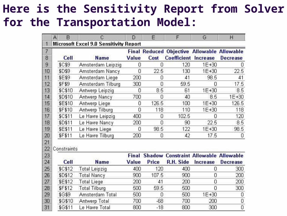
Here is the Sensitivity Report from Solver for the Transportation Model:

Variations on the Transportation ModelVariations on the Transportation Model
Suppose we now want to maximizemaximize the value of the objective function instead of minimizing it.
In this case, we would use the same model, but now the objective function coefficients define the contribution margins (i.e., unit returns) instead of unit costs.
In the Solver dialog, you would check the Max radio button before solving the problem.
Additionally, your interpretation of Solver’s Sensitivity Report would reflect the maximization of the objective function.
Solving Max Transportation ModelsSolving Max Transportation Models

Variations on the Transportation ModelVariations on the Transportation Model
When supply and demand are not equal, then the problem is unbalanced. There are two situations:
When supply is greater than demand:
When Supply and Demand DifferWhen Supply and Demand Differ
In this case, when all demand is satisfied, the remaining supply that was not allocated at each origin would appear as slack in the supply constraint for that origin.
Using inequalities in the constraints (as in the previous example) would not cause any problems in Solver.

Variations on the Transportation ModelVariations on the Transportation Model
In this case, the LP model has no feasible solution. However, there are two approaches to solving this problem:
1. Rewrite the supply constraints to be equalities and rewrite the demand constraints to be < .
Unfulfilled demand will appear as slack on each of the demand constraints when Solver optimizes the model.
When demand is greater than supply:

Variations on the Transportation ModelVariations on the Transportation Model
2. Revise the model to append a placeholder origin, called a dummy origin, with supply equal to the difference between total demand and total supply.
The purpose of the dummy origin is to make the problem balanced (total supply = total demand) so that Solver can solve it.
The cost of supplying any destination from this origin is zero.
Once solved, any supply allocated from this origin to a destination is interpreted as unfilled demand.

Variations on the Transportation ModelVariations on the Transportation Model
Certain routes in a transportation model may be unacceptable due to regional restrictions, delivery time, etc.
In this case, you can assign an arbitrarily large unit cost number (identified as M) to that route.
This will force Solver to eliminate the use of that route since the cost of using it would be much larger than that of any other feasible alternative.
Eliminating Unacceptable RoutesEliminating Unacceptable Routes
Choose M such that it will be larger than any other unit cost number in the model.

Variations on the Transportation ModelVariations on the Transportation Model
Generally, LP models do not produce integer solutions.
The exception to this is the Transportation model. In general:
Integer Valued SolutionsInteger Valued Solutions
If all of the supplies and demands in a If all of the supplies and demands in a transportation model have integer values, transportation model have integer values,
the optimal values of the decision variables the optimal values of the decision variables will also have integer values.will also have integer values.

Variations on the Transportation ModelVariations on the Transportation Model
Zeros in the Allowable Increase/Decrease columns for objective coefficients in the Sensitivity Report indicate that there are alternative optimal solutions.
Using Alternative Optima to Achieve Using Alternative Optima to Achieve Multiple ObjectivesMultiple Objectives
Using the AutoPower example, examine the effects of such occurrences.
Suppose that due to a potential trucker’s strike, you need to find a cheaper transportation schedule that also minimizes the cost of shipping motors out of Le Havre harbor. You would need to shift costs away from Le Havre to reduce AutoPower’s risk.

In this case, the presence of alternative optima would help avoid some of the risk without increasing total costs.From the previous solution, we find that there are an infinite number of alternative optima that produce a minimal cost of $121,450.
So, the original objective can then be recast as an additional total cost constraint, thereby allowing Solver to be given a new OV to minimize.

Here is the modified spreadsheet model.
Note the additional constraint $G$19 < $H$19.
Note that the new solution provides feasible alternatives (no more costly than the original solution), while minimizing Le Havre’s total costs (a shift of $18,000 to other routes).

The Assignment ModelThe Assignment ModelIn general, the Assignment model is the problem of determining the optimal assignment of n “indivisible” agents or objects to n tasks.For example, you might want to assign
Salespeople to sales territories
Computers to networks
Consultants to clients
Service representatives to service calls
Lawyers to cases
Commercial artists to advertising copy
The important constraint is that each person or The important constraint is that each person or machine be assigned to machine be assigned to one and only one taskone and only one task..

The Assignment ModelThe Assignment Model
We will use the AutoPower example to illustrate Assignment problems.
AutoPower Europe’s Auditing ProblemAutoPower Europe’s Auditing Problem
AutoPower’s European headquarters is in Brussels. This year, each of the four corporate vice-presidents will visit and audit one of the assembly plants in June. The plants are located in:
Leipzig, Germany
Liege, Belgium
Nancy, France
Tilburg, the Netherlands

The issues to consider in assigning the different vice-presidents to the plants are:
1. Matching the vice-presidents’ areas of expertise with the importance of specific problem areas in a plant.
2. The time the management audit will require and the other demands on each vice- president during the two-week interval.
3. Matching the language ability of a vice- president with the plant’s dominant language.
Keeping these issues in mind, first estimate the (opportunity) cost to AutoPower of sending each vice-president to each plant.

The following table lists the assignment costs in $000s for every vice-president/plant combination.
PLANTPLANT Leipzig Nancy Liege Leipzig Nancy Liege
TilburgTilburg V.P. (1) (2) (3) (4)V.P. (1) (2) (3) (4)
Finance (F)Finance (F) 24 10 21 11
Marketing (M)Marketing (M) 14 22 10 15
Operations (O)Operations (O) 15 17 20 19
Personnel (P)Personnel (P) 11 19 14 13
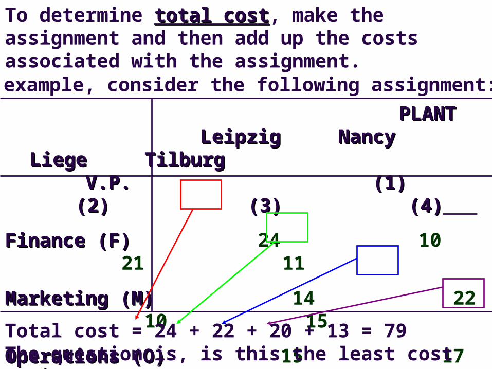
To determine total costtotal cost, make the assignment and then add up the costs associated with the assignment.
PLANTPLANT Leipzig Nancy Liege Leipzig Nancy Liege
TilburgTilburg V.P. (1) (2) (3) (4)V.P. (1) (2) (3) (4)
Finance (F)Finance (F) 24 10 21 11
Marketing (M)Marketing (M) 14 22 10 15
Operations (O)Operations (O) 15 17 20 19
Personnel (P)Personnel (P) 11 19 14 13
For example, consider the following assignment:
Total cost = 24 + 22 + 20 + 13 = 79The question is, is this the least cost assignment?

The Assignment ModelThe Assignment Model
Complete enumeration is the calculation of the total cost of each feasible assignment pattern in order to pick the assignment with the lowest total cost.
Solving by Complete EnumerationSolving by Complete Enumeration
This is not a problem when there are only a few rows and columns (e.g., vice-presidents and plants). However, complete enumeration can quickly become burdensome as the model grows large.

For example, determine the number of alternatives in the AutoPower (4x4) model. Consider assigning the vice-presidents in the order F, M, O, P.
1. F can be assigned to any of the 4 plants.
2. Once F is assigned, M can be assigned to any of the remaining 3 plants.
3. Now O can be assigned to any of the remaining 2 plants.4. P must be assigned to the only remaining plant.
There are 4 x 3 x 2 x 1 = 24 possible solutions. In general, if there are n rows and n columns, then there would be n(n-1)(n-2)(n-3)…(2)(1) = n! (n factorial) solutions. As n increases, n! increases rapidly. Therefore, this may not be the best method.

The Assignment ModelThe Assignment Model
For this model, let xij = number of V.P’s of type i assigned to plant jwhere i = F, M, O, P j = 1, 2, 3, 4
The LP Formulation and SolutionThe LP Formulation and Solution
Notice that this model is balanced since the total number of V.P.’s is equal to the total number of plants.
Remember, only one V.P. (supply) is needed at each plant (demand).

Here is the spreadsheet model using Excel
= C4*C10
=SUM (C10:F10)=SUM(C10:C13)
=SUM (C18:F18)
=SUM(C18:C21)
and solved with Solver:

As a result, the optimal assignment is:
PLANTPLANT Leipzig Nancy Liege Leipzig Nancy Liege
TilburgTilburg V.P. (1) (2) (3) (4)V.P. (1) (2) (3) (4)
Finance (F)Finance (F) 24 10 21 11
Marketing (M)Marketing (M) 14 22 10 15
Operations (O)Operations (O) 15 17 20 19
Personnel (P)Personnel (P) 11 19 14 13 Total Cost ($000’s) = 10 + 10 + 15 + 13 = 48

The Assignment ModelThe Assignment Model
The Assignment model is similar to the Transportation model with the exception that supply cannot be distributed to more than one destination.
Relation to the Transportation ModelRelation to the Transportation Model
In the Assignment model, all supplies and demands are one, and hence integers. Thus, Solver will not produce any fractional allocations.
As a result, in the Solver solution, each decision variable cell will either contain a 0 (no assignment) or a 1 (assignment made).
In general, the assignment model can be formulated In general, the assignment model can be formulated as a transportation model in which the supply at as a transportation model in which the supply at each origin and the demand at each destination = 1.each origin and the demand at each destination = 1.
The Assignment ModelThe Assignment Model
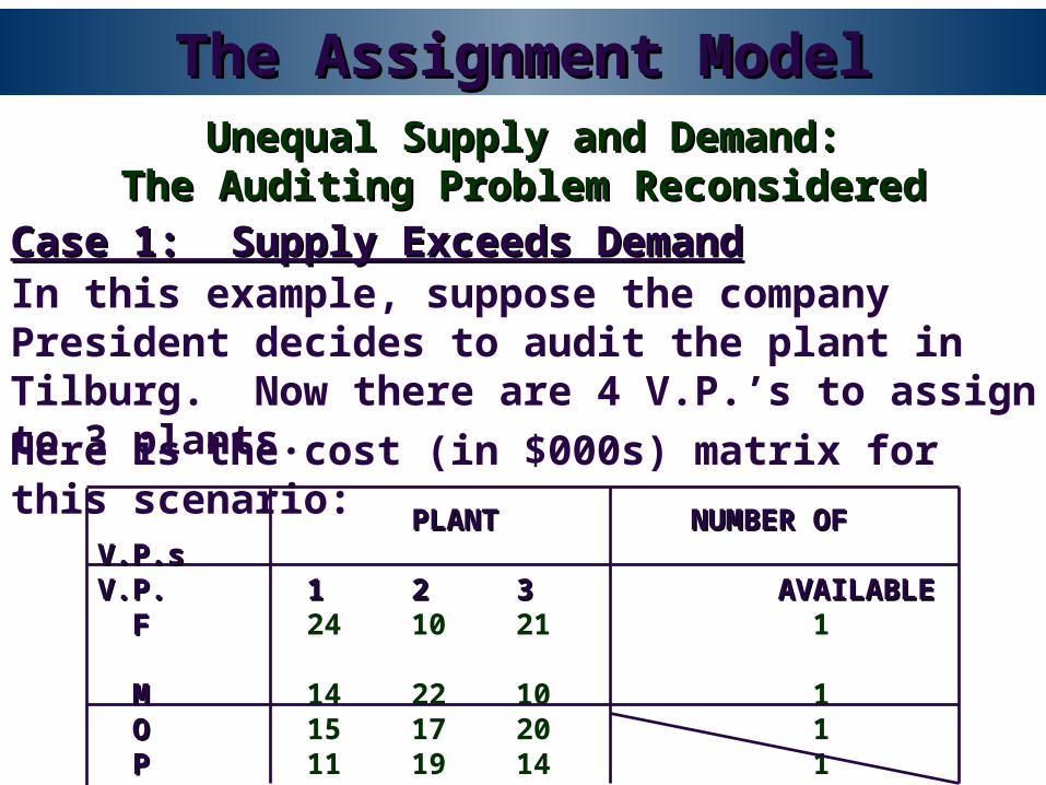
Case 1: Supply Exceeds DemandCase 1: Supply Exceeds Demand
Unequal Supply and Demand:Unequal Supply and Demand:The Auditing Problem ReconsideredThe Auditing Problem Reconsidered
In this example, suppose the company President decides to audit the plant in Tilburg. Now there are 4 V.P.’s to assign to 3 plants.
Here is the cost (in $000s) matrix for this scenario:
PLANTPLANT NUMBER OF V.P.s NUMBER OF V.P.sV.P.V.P. 11 22 33 AVAILABLE AVAILABLE FF 24 10 21 1 MM 14 22 10 1 OO 15 17 20 1 PP 11 19 14 1No. of V.P.s No. of V.P.s 4RequiredRequired 1 1 1 3

To formulate this model, simply drop the constraint that required a V.P. at plant 4 and Solve:
Note that one of the V.P.s has not been assigned to a plant.

The Assignment ModelThe Assignment Model
Case 2: Demand Exceeds SupplyCase 2: Demand Exceeds Supply
Unequal Supply and Demand:Unequal Supply and Demand:The Auditing Problem ReconsideredThe Auditing Problem Reconsidered
In this example, assume that the V.P. of Personnel is unable to participate in the European audit. Now the cost matrix is as follows:
PLANTPLANT NUMBER OF V.P.sNUMBER OF V.P.sV.P.V.P. 11 22 33 44 AVAILABLE AVAILABLE
FF 24 10 21 11 1 MM 14 22 10 15 1 OO 15 17 20 19 1
No. of V.P.s No. of V.P.s 3RequiredRequired 1 1 1 1 4

Demand > Supply: Adding a Dummy V.P.
In this form, the model is infeasible.
To fix this, you can1. Modify the inequalities in the constraints
(similar to the Transportation example)2. Add a dummy V.P. as a placeholder to the
cost matrix (shown below).
PLANTPLANT NUMBER OF V.P.sNUMBER OF V.P.sV.P.V.P. 11 22 33 44 AVAILABLE AVAILABLE
FF 24 10 21 11 1 MM 14 22 10 15 1 OO 15 17 20 19 1DummyDummy 0 0 0 0 1
No. of V.P.s No. of V.P.s 4RequiredRequired 1 1 1 1 4
Zero cost to assign the dummyDummy supply; now supply = demand
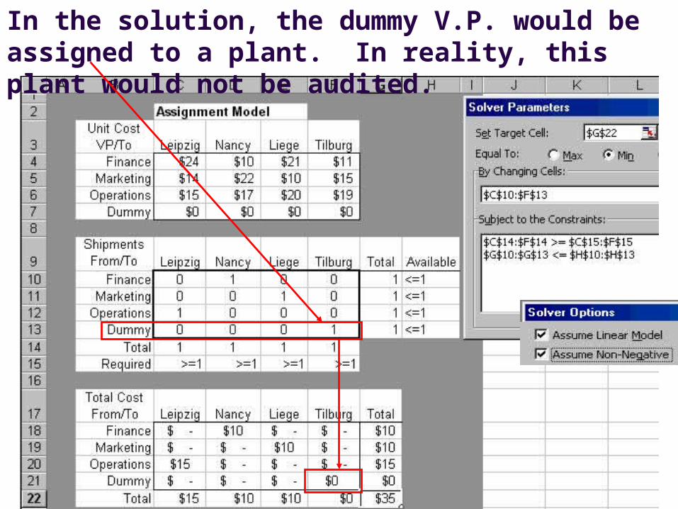
In the solution, the dummy V.P. would be assigned to a plant. In reality, this plant would not be audited.

The Assignment ModelThe Assignment Model
In this Assignment model, the response from each assignment is a profit rather than a cost.
Maximization ModelsMaximization Models
For example, AutoPower must now assign four new salespeople to three territories in order to maximize maximize profitprofit.
The effect of assigning any salesperson to a territory is measured by the anticipated marginal increase in profit contribution due to the assignment.
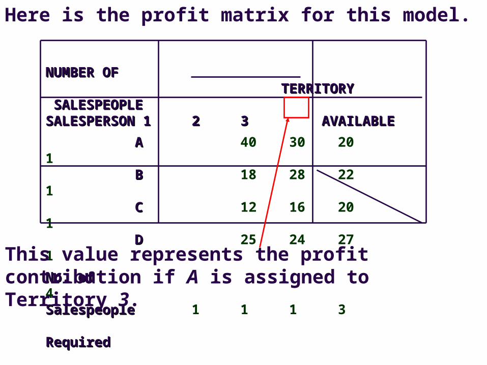
Here is the profit matrix for this model.
NUMBER OFNUMBER OF TERRITORY TERRITORY SALESPEOPLE SALESPEOPLE
SALESPERSONSALESPERSON 11 22 3 AVAILABLE3 AVAILABLE
AA 40 30 20 1 BB 18 28 22 1 CC 12 16 20 1 DD 25 24 27 1
No. of No. of 4 SalespeopleSalespeople 1 1 1 3 RequiredRequired
This value represents the profit contribution if A is assigned to Territory 3.
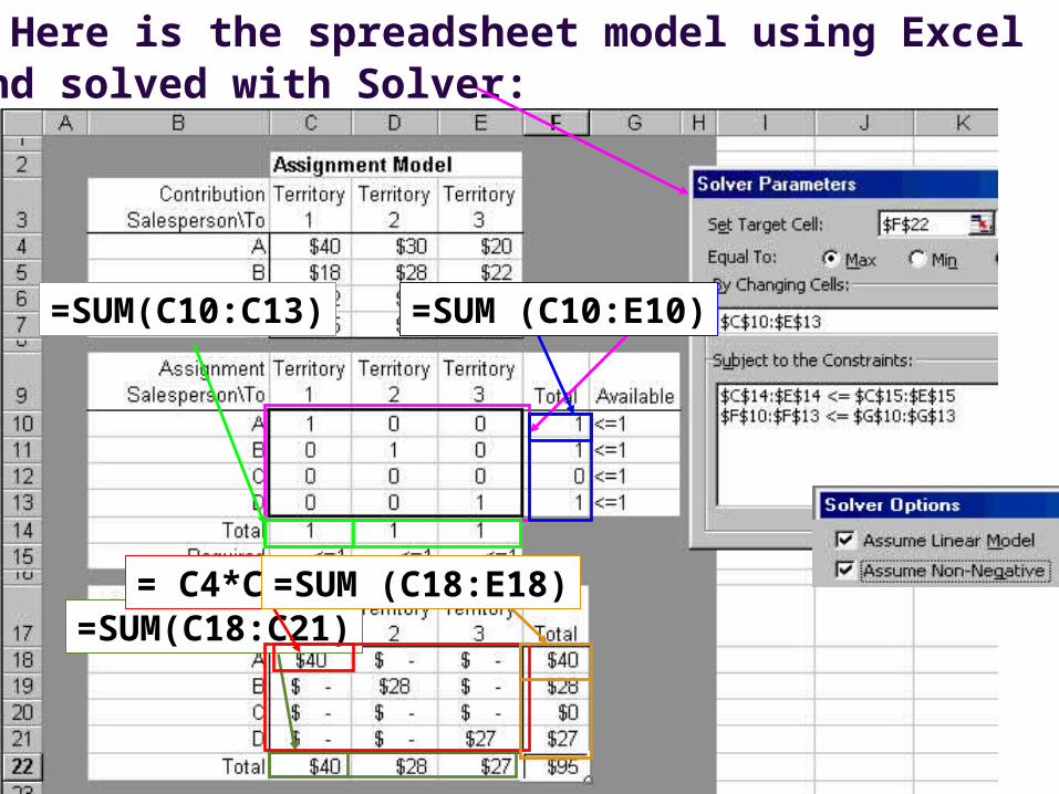
and solved with Solver:
=SUM(C18:C21)
Here is the spreadsheet model using Excel
= C4*C10
=SUM (C10:E10)=SUM(C10:C13)
=SUM (C18:E18)

The Assignment ModelThe Assignment Model
Certain assignments in the model may be unacceptable for various reasons.
Situations with Unacceptable AssignmentsSituations with Unacceptable Assignments
In this case, you can assign an arbitrarily large unit cost (or small unit profit) number to that assignment.
This will force Solver to eliminate the use of that assignment since, for example, the cost of making that assignment would be much larger than that of any other feasible alternative.

The Media Selection ModelThe Media Selection Model
Advertising agencies use Media SelectionMedia Selection models to develop effective advertising campaigns.
The basic question that they try to answer is:How many “insertions” (ads) should the firm purchase in each of several possible media (e.g., radio, TV, newspapers, magazines, and Internet Web pages)?
Constraints on the decision maker are typically:advertising budget
the number of ads in each media
other “rules of thumb” from management

The Media Selection ModelThe Media Selection Model
The law of diminishing returnslaw of diminishing returns may also influence the Media Selection decision. In other words, the effectiveness of an ad decreases as the number of exposures in a medium increases during a specified period of time.
The objective functionobjective function of this model is unusual. Conceptually, the model should find the advertising campaign that maximizes demand and satisfies the budget and other constraints.
However, the approach most often used is to measure the response to an ad in a medium in terms of exposure unitsexposure units.

The Media Selection ModelThe Media Selection Model
An exposure unitexposure unit is a subjective measure based on:
An exposure unit can be thought of as a kind of economic utility.
So the goal is to maximize the total exposure units, taking into account other properties of the model.
The quality of the ad
The desirability of the potential market
In other words, it is an arbitrary measure of the “goodness” of an ad.
The Media Selection ModelThe Media Selection Model
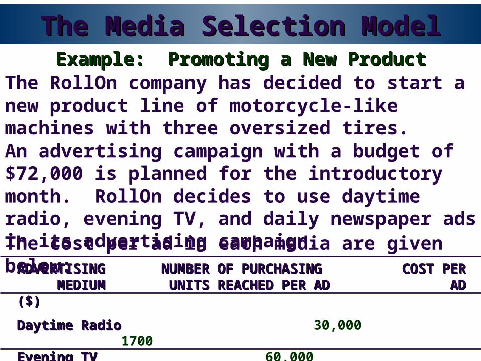
The RollOn company has decided to start a new product line of motorcycle-like machines with three oversized tires.
Example: Promoting a New ProductExample: Promoting a New Product
An advertising campaign with a budget of $72,000 is planned for the introductory month. RollOn decides to use daytime radio, evening TV, and daily newspaper ads in its advertising campaign.
ADVERTISINGADVERTISING NUMBER OF PURCHASINGNUMBER OF PURCHASING COST PERCOST PER MEDIUMMEDIUM UNITS REACHED PER AD UNITS REACHED PER AD AD ($) AD ($)
Daytime RadioDaytime Radio 30,000 1700Evening TVEvening TV 60,000 2800Daily NewspaperDaily Newspaper 45,000 1200
The cost per ad in each media are given below:

Total Exposures vs. Number of Radio Ads
0
200
400
600
800
1000
1200
0 5 10 15 20 25
Number of Ads
To
tal E
xpo
su
res
Slope = 60
It is assumed that each of the
first 10 radio ads has a value of 60
exposure units,
The Media Selection ModelThe Media Selection Model
RollOn arbitrarily selects a scale from 0 to 100 for each ad offering.
Example: Promoting a New ProductExample: Promoting a New Product
and each radio ad after the first
10 is rated as having 40
exposures.
Slope = 40

The previous graph shows that radio adds suffer from diminishing returns (as evidenced by the change in slope from 60 to 40).
RollOn subjectively determines that the first radio ads are more effective than later ones. In addition, they feel that the same situation will occur with TV and newspaper ads.
The exposures per ad for each medium are given below:
ADVERTISINGADVERTISING ALL FOLLOWING ALL FOLLOWING MEDIUMMEDIUM FIRST 10 ADS FIRST 10 ADS ADS ADS
Daytime RadioDaytime Radio 60 40Evening TVEvening TV 80 55Daily NewspaperDaily Newspaper 70 35

Total Exposures vs. Number of Ads
0
200
400
600
800
1000
1200
1400
0 10 20 30
Number of Ads
To
tal E
xpo
su
res
TV
Newspaper
Radio
55
8070
35
60
40
Here is a plot of the total exposures as a function of the number of ads in each medium.

RollOn wants to ensure that the ad campaign will satisfy the following important criteria:
1. No more than 25 ads per medium2. A total of 1,800,000 purchasing units must be reached across all media3. At least ¼ of the ads must appear on TV (blending requirement)
Now, to model this Media Selection model as an LP model, let
x1 = no. of daytime radio ads up to the first 10y1 = no. of daytime radio ads after the first 10x2 = no. of evening TV ads up to the first 10y2 = no. of evening TV ads after the first 10x3 = no. of newspaper ads up to the first 10
y3 = no. of newspaper ads after the first 10

The objective functionobjective function is:
Max 60x1 + 40y1 + 80x2 + 55y2 + 70x3 + 35y3
To determine the constraints,constraints, remember:
x1 + y1 = total radio ads
x2 + y2 = total TV ads
x3 + y3 = total newspaper ads
Also remember that the total advertising expenditure cannot exceed $72,000 and the cost of each radio ad is $1700, each TV ad is $2800 and each newspaper ad is $1200. Therefore, the total expenditure constraint is:
1700x1 + 1700y1 + 2800x2 + 2800y2 + 1200x3 + 1200y3 < 72,000
No. exposures

The constraintsconstraints are:
x1 + y1 < 25
1700x1 + 1700y1 + 2800x2 + 2800y2 + 1200x3 + 1200y3 < 72,000
x2 + y2 < 25x3 + y3 < 25
30,000x1 + 30,000y1 + 60,000x2 + 60,000y2 + 45,000x3 + 45,000y3 > 1,800,000
Total advertising expenditure less than $72,000:
No more than 25 ads in a single medium:
The entire campaign must reach at least 1,800,000 purchasing units:
Cost per ad
No. purchasing units per ad

Blending Constraint (at least ¼ of the ads must appear on event TV) :
x2 + y2
x1 + y1 + x2 + y2 + x3 + y3
> ¼
Using this constraint in Excel will produce a Solver “Conditions for Assume Linear Model are not Satisfied” error message. You can make this constraint linear by multiplying out the denominator:
x2 + y2 > .25(x1 + y1 + x2 + y2 + x3 + y3 )

Here is the Solver setup:
Here is the Excel spreadsheet model after Solving:
= M3*F5 =C5*I5
= C3*C9 = C3*I9
End of Part 1Please continue to Part 2