Embed Size (px)
Citation preview

Decision Making Under Uncertainty
Jim LittleDecision 1
Nov 17 2014
Lecture Overview
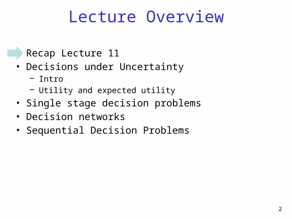
• Recap Lecture 11• Decisions under Uncertainty
– Intro– Utility and expected utility
• Single stage decision problems• Decision networks• Sequential Decision Problems
2
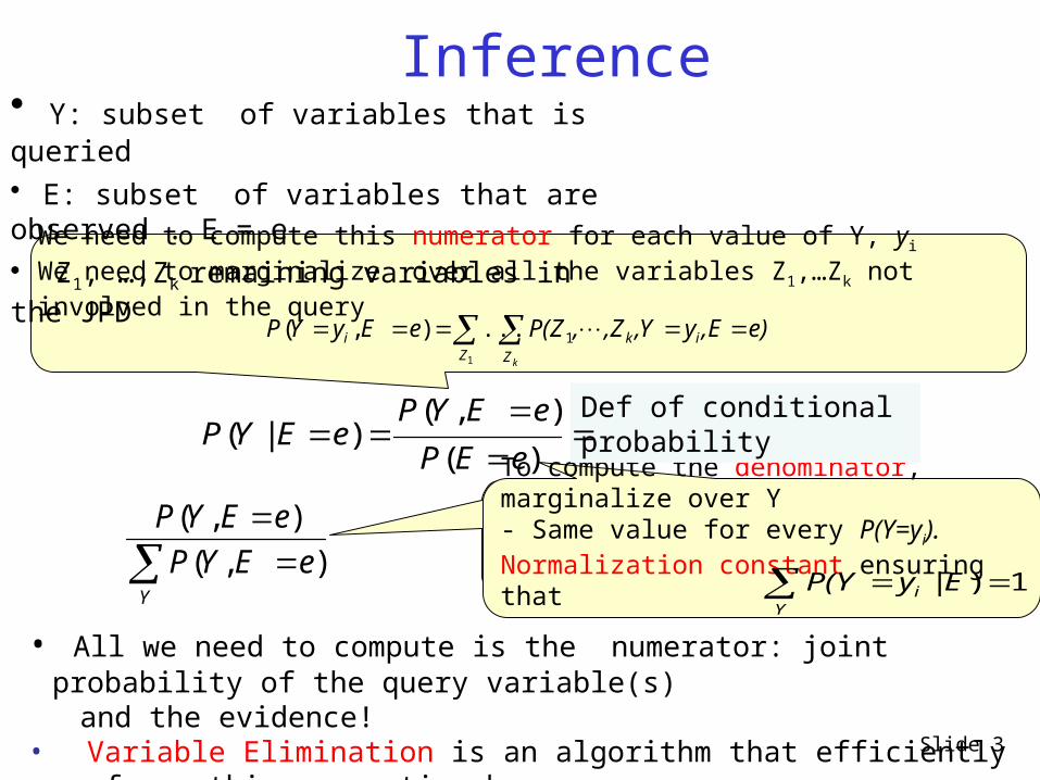
Inference
)(
),()|(
eEP
eEYPeEYP
• All we need to compute is the numerator: joint probability of the query variable(s) and the evidence!• Variable Elimination is an algorithm that efficiently performs this operation by casting it as operations between factors - introduced next
Y
eEYP
eEYP
),(
),(
We need to compute this numerator for each value of Y, yi
We need to marginalize over all the variables Z1,…Zk not involved in the query
kZik
Zi e),Ey,Y,Z,P(ZeEyYP 1
1
...),(
To compute the denominator, marginalize over Y- Same value for every P(Y=yi). Normalization constant ensuring that
Yi EyP(Y 1)|
Def of conditional probability
• Y: subset of variables that is queried
• E: subset of variables that are observed . E = e
• Z1, …,Zk remaining variables in the JPD
Slide 3
4
X Y Z val
t t t 0.1
t t f 0.9
t f t 0.2
t f f 0.8
f t t 0.4
f t f 0.6
f f t 0.3
f f f 0.7
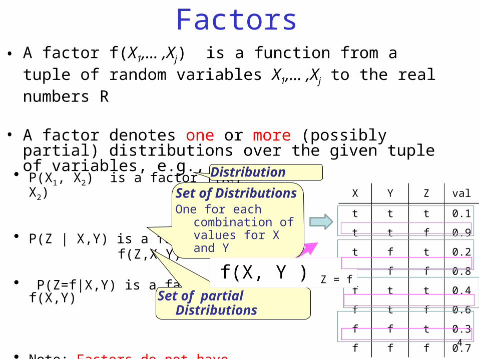
Factors• A factor f(X1,… ,Xj) is a function from a tuple of random
variables X1,… ,Xj to the real numbers R
• A factor denotes one or more (possibly partial) distributions over the given tuple of variables, e.g.,
• P(X1, X2) is a factor f(X1, X2)
• P(Z | X,Y) is a factor f(Z,X,Y)
• P(Z=f|X,Y) is a factor f(X,Y)
• Note: Factors do not have to sum to one
Distribution
Set of DistributionsOne for each combination
of values for X and Y
Set of partial Distributions
f(X, Y ) Z = f
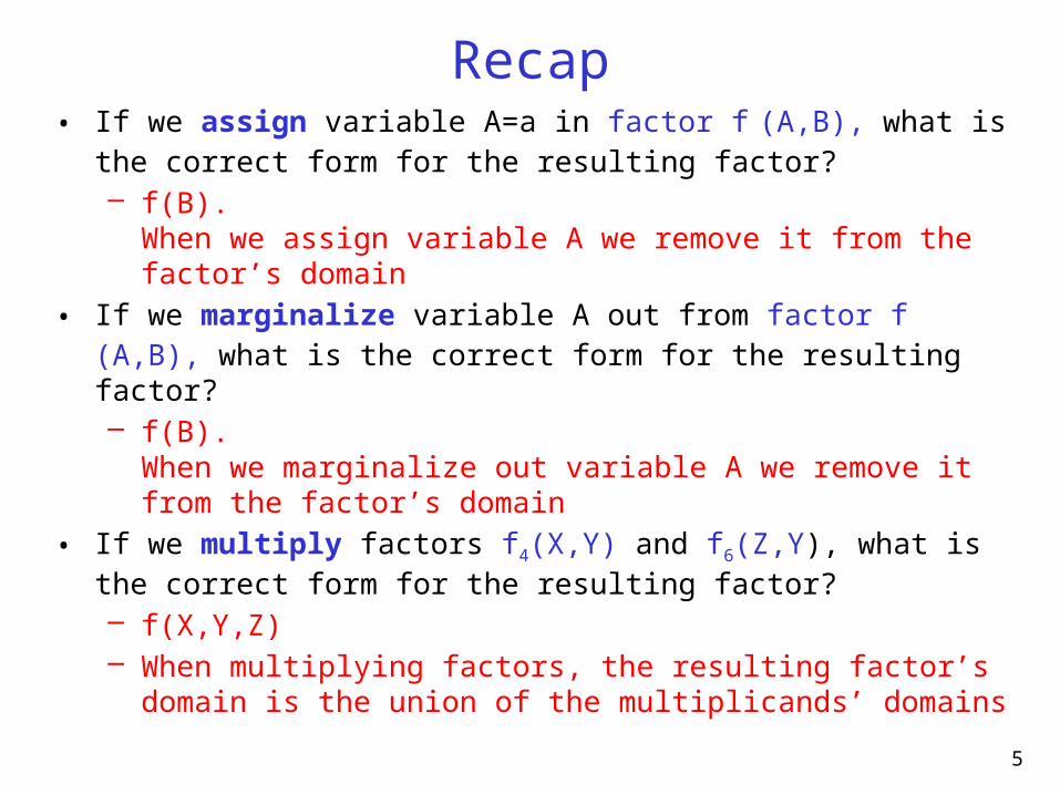
Recap• If we assign variable A=a in factor f (A,B), what is the correct form for the
resulting factor?– f(B).
When we assign variable A we remove it from the factor’s domain
• If we marginalize variable A out from factor f (A,B), what is the correct form for the resulting factor?– f(B).
When we marginalize out variable A we remove it from the factor’s domain
• If we multiply factors f4(X,Y) and f6(Z,Y), what is the correct form for the resulting factor?– f(X,Y,Z)– When multiplying factors, the resulting factor’s domain is the union of the
multiplicands’ domains
5
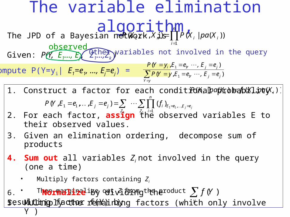
The variable elimination algorithm,
1. Construct a factor for each conditional probability.
2. For each factor, assign the observed variables E to their observed values.
3. Given an elimination ordering, decompose sum of products
4. Sum out all variables Zi not involved in the query (one a time)
• Multiply factors containing Zi
• Then marginalize out Zi from the product
5. Multiply the remaining factors (which only involve Y )
6. Normalize by dividing the resulting factor f(Y) by y
Yf )(
To compute P(Y=yi| E1=e1, …, Ej=ej) =
The JPD of a Bayesian network is
Given: P(Y, E1…, Ej , Z1…,Zk )
))(|( ) , ,P(1
1
n
iiin XpaXPXX
))(,())(|( iiiii XpaXfXpaXP
1
11 ,,1
11 )(),,,(Z
eEeE
n
ii
Zjj jj
k
feEeEYP
observedOther variables not involved in the query
yYjj
jji
e, E, eEyYP
e, E, eEyYP
),(
),(
11
11
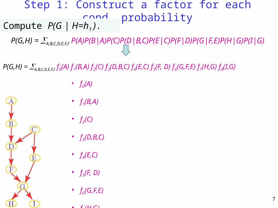
Step 1: Construct a factor for each cond. probability
P(G,H) = A,B,C,D,E,F,I P(A)P(B|A)P(C)P(D|B,C)P(E|C)P(F|D)P(G|F,E)P(H|G)P(I|G)
P(G,H) = A,B,C,D,E,F,I f0(A) f1(B,A) f2(C) f3(D,B,C) f4(E,C) f5(F, D) f6(G,F,E) f7(H,G) f8(I,G)
• f0(A)
• f1(B,A)
• f2(C)
• f3(D,B,C)
• f4(E,C)
• f5(F, D)
• f6(G,F,E)
• f7(H,G)
• f8(I,G)
Compute P(G | H=h1 ).
7
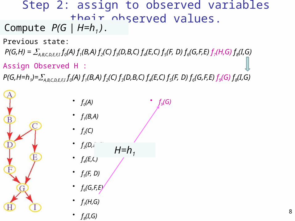
Previous state:
P(G,H) = A,B,C,D,E,F,I f0(A) f1(B,A) f2(C) f3(D,B,C) f4(E,C) f5(F, D) f6(G,F,E) f7(H,G) f8(I,G)
Assign Observed H :
• f9(G)• f0(A)
• f1(B,A)
• f2(C)
• f3(D,B,C)
• f4(E,C)
• f5(F, D)
• f6(G,F,E)
• f7(H,G)
• f8(I,G)
Step 2: assign to observed variables their observed values.
P(G,H=h1)=A,B,C,D,E,F,I f0(A) f1(B,A) f2(C) f3(D,B,C) f4(E,C) f5(F, D) f6(G,F,E) f9(G) f8(I,G)
Compute P(G | H=h1 ).
H=h1
8
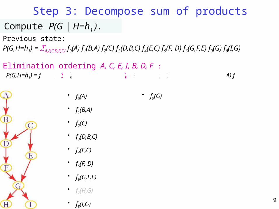
Step 3: Decompose sum of products
Previous state: P(G,H=h1) = A,B,C,D,E,F,I f0(A) f1(B,A) f2(C) f3(D,B,C) f4(E,C) f5(F, D) f6(G,F,E) f9(G) f8(I,G)
Elimination ordering A, C, E, I, B, D, F : P(G,H=h1) = f9(G) F D f5(F, D) B I f8(I,G) E f6(G,F,E) C f2(C) f3(D,B,C) f4(E,C) A f0(A) f1(B,A)
• f9(G)• f0(A)
• f1(B,A)
• f2(C)
• f3(D,B,C)
• f4(E,C)
• f5(F, D)
• f6(G,F,E)
• f7(H,G)
• f8(I,G)
Compute P(G | H=h1 ).
9
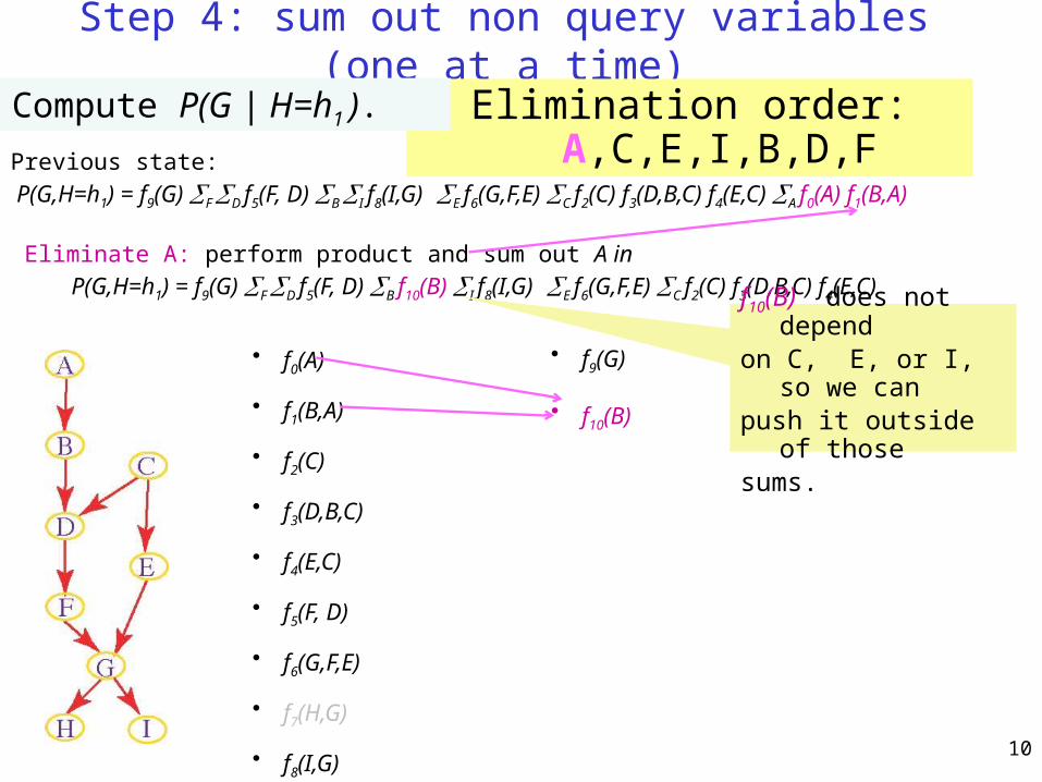
Step 4: sum out non query variables (one at a time)
Previous state:
P(G,H=h1) = f9(G) F D f5(F, D) B I f8(I,G) E f6(G,F,E) C f2(C) f3(D,B,C) f4(E,C) A f0(A) f1(B,A)
Eliminate A: perform product and sum out A in
P(G,H=h1) = f9(G) F D f5(F, D) B f10(B) I f8(I,G) E f6(G,F,E) C f2(C) f3(D,B,C) f4(E,C)
• f9(G)• f0(A)
• f1(B,A)
• f2(C)
• f3(D,B,C)
• f4(E,C)
• f5(F, D)
• f6(G,F,E)
• f7(H,G)
• f8(I,G)
• f10(B)
Elimination order: A,C,E,I,B,D,FCompute P(G | H=h1 ).
f10(B) does not depend on C, E, or I, so we can push it outside of those sums.
10
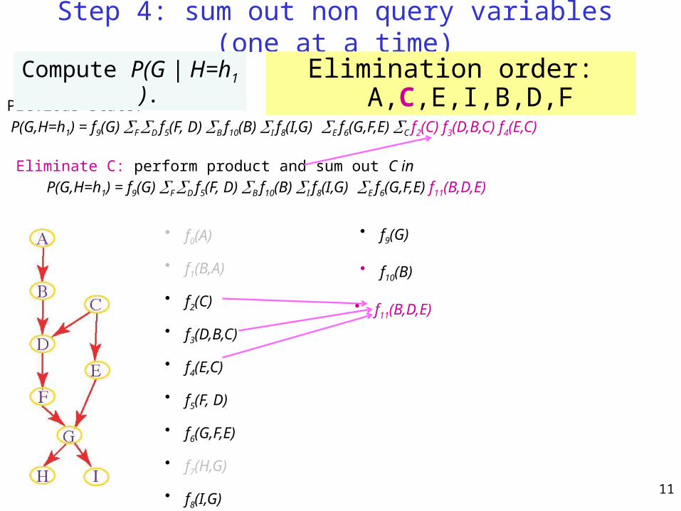
Step 4: sum out non query variables (one at a time)
Previous state:
P(G,H=h1) = f9(G) F D f5(F, D) B f10(B) I f8(I,G) E f6(G,F,E) C f2(C) f3(D,B,C) f4(E,C)
Eliminate C: perform product and sum out C in
P(G,H=h1) = f9(G) F D f5(F, D) B f10(B) I f8(I,G) E f6(G,F,E) f11(B,D,E)
• f9(G)• f0(A)
• f1(B,A)
• f2(C)
• f3(D,B,C)
• f4(E,C)
• f5(F, D)
• f6(G,F,E)
• f7(H,G)
• f8(I,G)
• f10(B)
Compute P(G | H=h1 ). Elimination order: A,C,E,I,B,D,F
• f11(B,D,E)
11
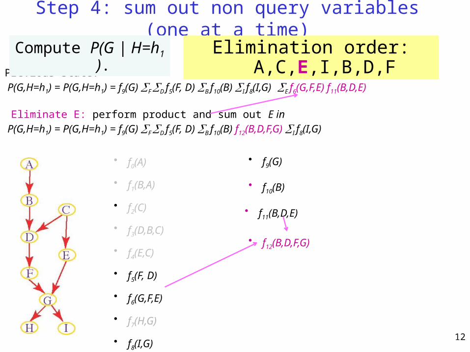
Step 4: sum out non query variables (one at a time)
Previous state:
P(G,H=h1) = P(G,H=h1) = f9(G) F D f5(F, D) B f10(B) I f8(I,G) E f6(G,F,E) f11(B,D,E)
Eliminate E: perform product and sum out E in
P(G,H=h1) = P(G,H=h1) = f9(G) F D f5(F, D) B f10(B) f12(B,D,F,G) I f8(I,G)
• f9(G)• f0(A)
• f1(B,A)
• f2(C)
• f3(D,B,C)
• f4(E,C)
• f5(F, D)
• f6(G,F,E)
• f7(H,G)
• f8(I,G)
• f10(B)
Compute P(G | H=h1 ). Elimination order: A,C,E,I,B,D,F
• f11(B,D,E)
• f12(B,D,F,G)
12
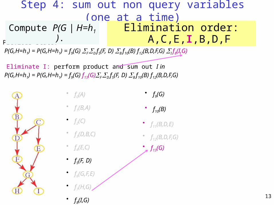
Previous state:
P(G,H=h1) = P(G,H=h1) = f9(G) F D f5(F, D) B f10(B) f12(B,D,F,G) I f8(I,G)
Eliminate I: perform product and sum out I in
P(G,H=h1) = P(G,H=h1) = f9(G) f13(G)F D f5(F, D) B f10(B) f12(B,D,F,G)
• f9(G)• f0(A)
• f1(B,A)
• f2(C)
• f3(D,B,C)
• f4(E,C)
• f5(F, D)
• f6(G,F,E)
• f7(H,G)
• f8(I,G)
• f10(B)
Elimination order: A,C,E,I,B,D,F
• f11(B,D,E)
• f12(B,D,F,G)
• f13(G)
Step 4: sum out non query variables (one at a time)
Compute P(G | H=h1 ).
13
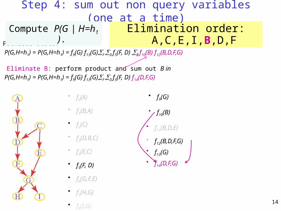
Previous state:
P(G,H=h1) = P(G,H=h1) = f9(G) f13(G)F D f5(F, D) B f10(B) f12(B,D,F,G)
Eliminate B: perform product and sum out B in
P(G,H=h1) = P(G,H=h1) = f9(G) f13(G)F D f5(F, D) f14(D,F,G)
• f9(G)• f0(A)
• f1(B,A)
• f2(C)
• f3(D,B,C)
• f4(E,C)
• f5(F, D)
• f6(G,F,E)
• f7(H,G)
• f8(I,G)
• f10(B)
Elimination order: A,C,E,I,B,D,F
• f11(B,D,E)
• f12(B,D,F,G)
• f13(G)
• f14(D,F,G)
Step 4: sum out non query variables (one at a time)
Compute P(G | H=h1 ).
14
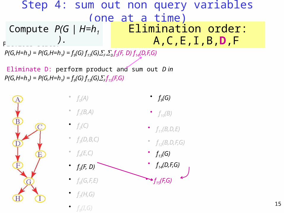
Previous state:
P(G,H=h1) = P(G,H=h1) = f9(G) f13(G)F D f5(F, D) f14(D,F,G)
Eliminate D: perform product and sum out D in
P(G,H=h1) = P(G,H=h1) = f9(G) f13(G)F f15(F,G)
• f9(G)• f0(A)
• f1(B,A)
• f2(C)
• f3(D,B,C)
• f4(E,C)
• f5(F, D)
• f6(G,F,E)
• f7(H,G)
• f8(I,G)
• f10(B)
Elimination order: A,C,E,I,B,D,F
• f11(B,D,E)
• f12(B,D,F,G)
• f13(G)
• f14(D,F,G)
• f15(F,G)
Step 4: sum out non query variables (one at a time)
Compute P(G | H=h1 ).
15
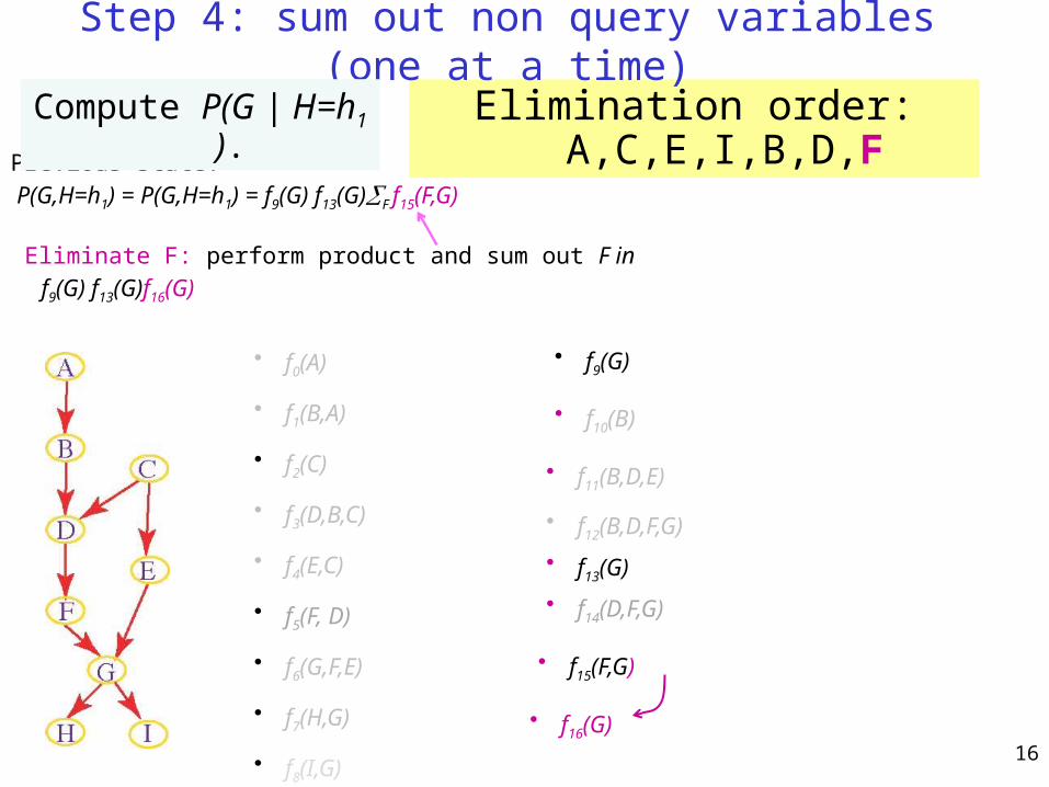
Previous state:
P(G,H=h1) = P(G,H=h1) = f9(G) f13(G)F f15(F,G)
Eliminate F: perform product and sum out F in
f9(G) f13(G)f16(G)
• f9(G)• f0(A)
• f1(B,A)
• f2(C)
• f3(D,B,C)
• f4(E,C)
• f5(F, D)
• f6(G,F,E)
• f7(H,G)
• f8(I,G)
• f10(B)
Elimination order: A,C,E,I,B,D,F
• f11(B,D,E)
• f12(B,D,F,G)
• f13(G)
• f14(D,F,G)
• f15(F,G)
• f16(G)
Step 4: sum out non query variables (one at a time)
Compute P(G | H=h1 ).
16
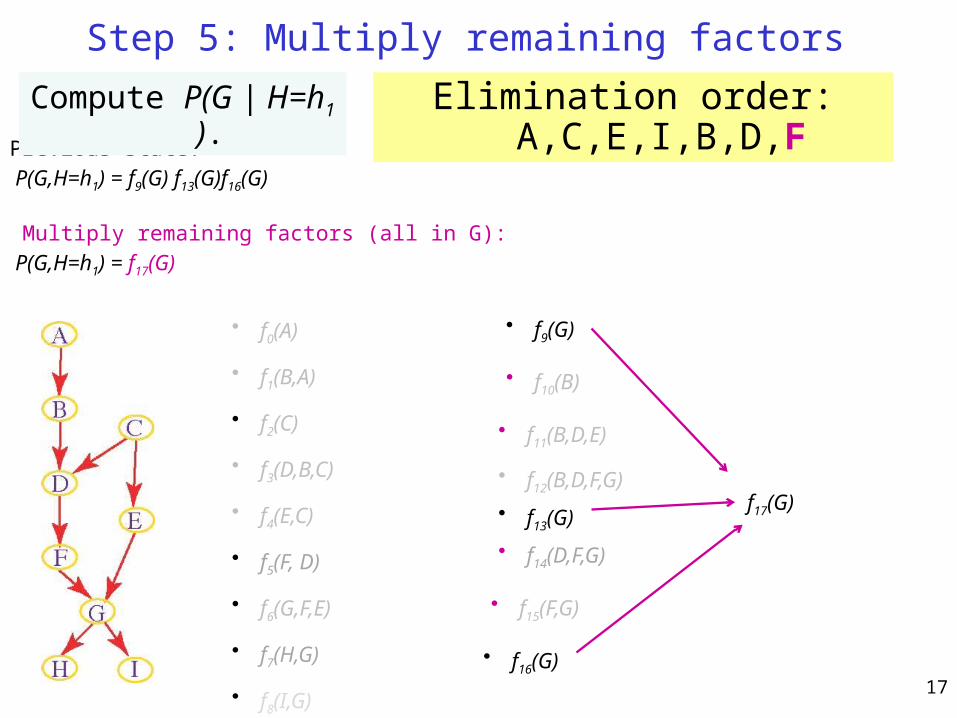
Step 5: Multiply remaining factors
Previous state:
P(G,H=h1) = f9(G) f13(G)f16(G)
Multiply remaining factors (all in G):
P(G,H=h1) = f17(G)
• f9(G)• f0(A)
• f1(B,A)
• f2(C)
• f3(D,B,C)
• f4(E,C)
• f5(F, D)
• f6(G,F,E)
• f7(H,G)
• f8(I,G)
• f10(B)
Compute P(G | H=h1 ). Elimination order: A,C,E,I,B,D,F
• f11(B,D,E)
• f12(B,D,F,G)
• f13(G)
• f14(D,F,G)
• f15(F,G)
• f16(G)
f17(G)
17
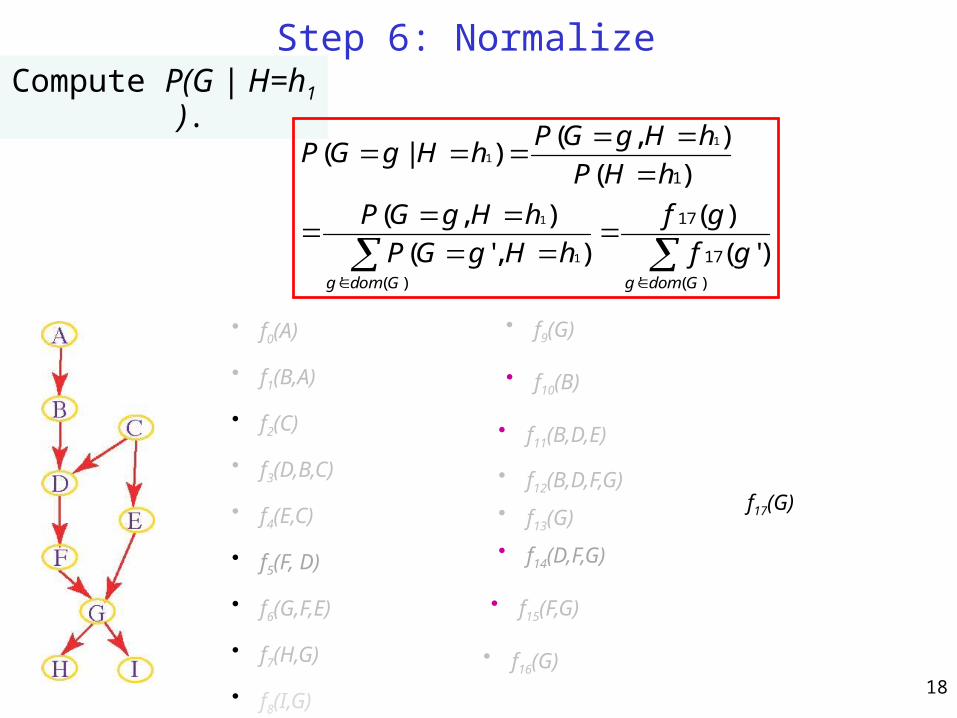
Step 6: Normalize
• f9(G)• f0(A)
• f1(B,A)
• f2(C)
• f3(D,B,C)
• f4(E,C)
• f5(F, D)
• f6(G,F,E)
• f7(H,G)
• f8(I,G)
• f10(B)
Compute P(G | H=h1 ).
• f11(B,D,E)
• f12(B,D,F,G)
• f13(G)
• f14(D,F,G)
• f15(F,G)
• f16(G)
f17(G)
)('
17
17
)('
1
)'(
)(
),'(
),(
)(
),()|(
1
1
1
1
GdomgGdomg
gf
gf
hHgGP
hHgGP
hHP
hHgGPhHgGP
18
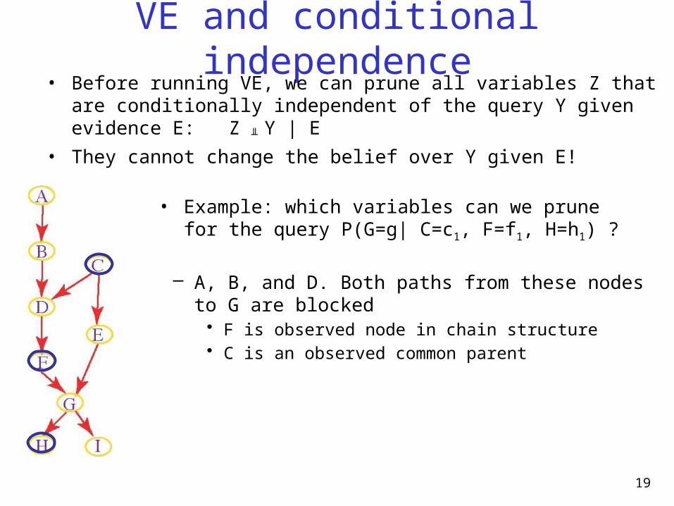
VE and conditional independence• Before running VE, we can prune all variables Z that are conditionally
independent of the query Y given evidence E: Z ╨ Y | E
• They cannot change the belief over Y given E!
19
• Example: which variables can we prune for the query P(G=g| C=c1, F=f1, H=h1) ?
– A, B, and D. Both paths from these nodes to G are blocked • F is observed node in chain structure• C is an observed common parent
20
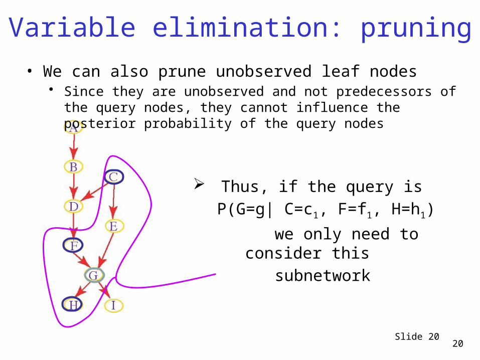
Variable elimination: pruning
Slide 20
Thus, if the query is
P(G=g| C=c1, F=f1, H=h1)
we only need to consider this
subnetwork
• We can also prune unobserved leaf nodes• Since they are unobserved and not predecessors of the query nodes, they
cannot influence the posterior probability of the query nodes
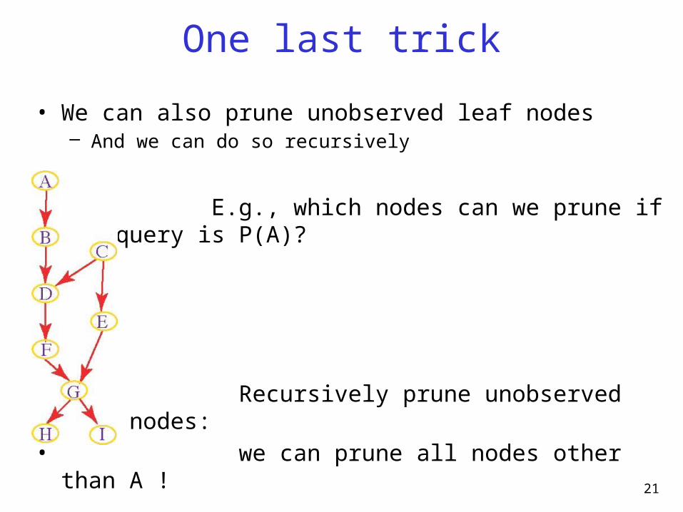
One last trick
• We can also prune unobserved leaf nodes– And we can do so recursively
• E.g., which nodes can we prune if the query is P(A)?
• Recursively prune unobserved leaf nodes:• we can prune all nodes other than A !
21
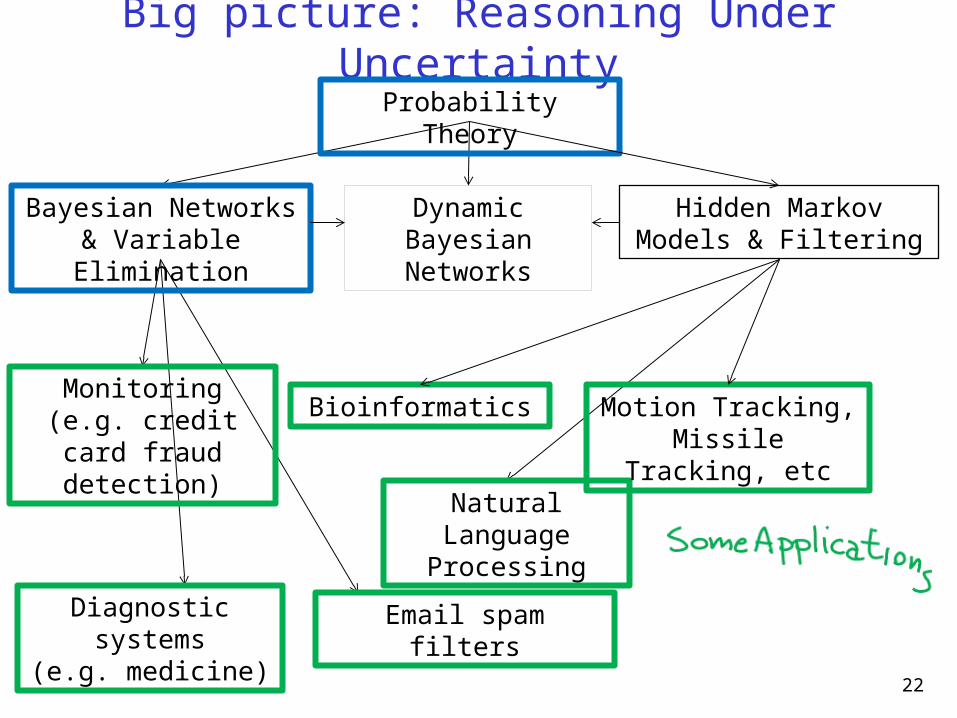
Bioinformatics
Big picture: Reasoning Under Uncertainty
Dynamic Bayesian Networks
Hidden Markov Models & Filtering
Probability Theory
Bayesian Networks & Variable Elimination
Natural Language Processing
Email spam filters
Motion Tracking,Missile Tracking,
etc
Monitoring(e.g. credit card fraud detection)
Diagnostic systems
(e.g. medicine)22
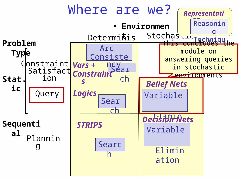
Where are we?• Environment
Problem Type
Query
Planning
Deterministic Stochastic
Constraint Satisfaction Search
Arc Consistency
Search
Search
Logics
STRIPS
Vars + Constraints
Variable
Elimination
Belief Nets
Decision Nets
Static
Sequential
Representation
ReasoningTechnique
Variable
Elimination
This concludes the module on answering queries in stochastic environments
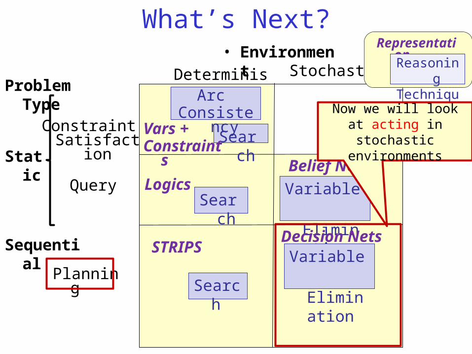
What’s Next?• Environment
Problem Type
Query
Planning
Deterministic Stochastic
Constraint Satisfaction Search
Arc Consistency
Search
Search
Logics
STRIPS
Vars + Constraints
Variable
Elimination
Belief Nets
Decision Nets
Static
Sequential
Representation
ReasoningTechnique
Variable
Elimination
Now we will look at acting in stochastic environments
Lecture Overview
• Recap Lecture 11• Decisions under Uncertainty
– Intro– Utility and expected utility
• Single stage decision problems• Decision networks• Sequential Decision Problems
25
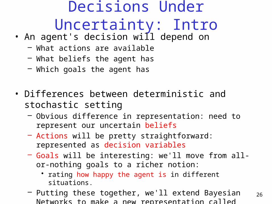
Decisions Under Uncertainty: Intro• An agent's decision will depend on
– What actions are available– What beliefs the agent has– Which goals the agent has
• Differences between deterministic and stochastic setting– Obvious difference in representation: need to represent our uncertain
beliefs– Actions will be pretty straightforward: represented as decision variables– Goals will be interesting: we'll move from all-or-nothing goals to a richer
notion: • rating how happy the agent is in different situations.
– Putting these together, we'll extend Bayesian Networks to make a new representation called Decision Networks
26
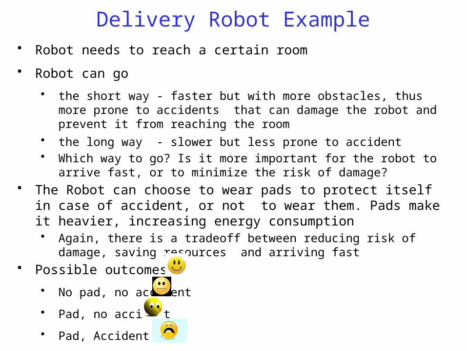
Delivery Robot Example• Robot needs to reach a certain room
• Robot can go
• the short way - faster but with more obstacles, thus more prone to accidents that can damage the robot and prevent it from reaching the room
• the long way - slower but less prone to accident• Which way to go? Is it more important for the robot to arrive fast, or to minimize
the risk of damage?• The Robot can choose to wear pads to protect itself in case of accident, or not
to wear them. Pads make it heavier, increasing energy consumption• Again, there is a tradeoff between reducing risk of damage, saving resources and
arriving fast• Possible outcomes
• No pad, no accident
• Pad, no accident
• Pad, Accident
• No pad, accident
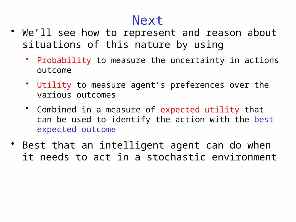
Next• We’ll see how to represent and reason about situations of this
nature by using
• Probability to measure the uncertainty in actions outcome
• Utility to measure agent’s preferences over the various outcomes
• Combined in a measure of expected utility that can be used to identify the action with the best expected outcome
• Best that an intelligent agent can do when it needs to act in a stochastic environment
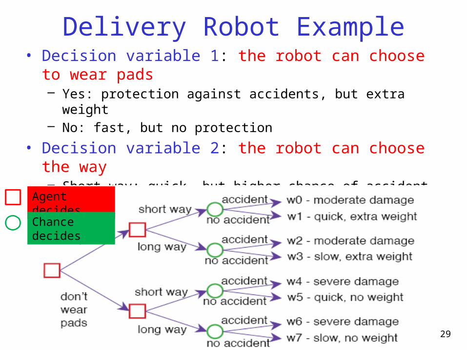
Delivery Robot Example• Decision variable 1: the robot can choose to wear pads
– Yes: protection against accidents, but extra weight– No: fast, but no protection
• Decision variable 2: the robot can choose the way– Short way: quick, but higher chance of accident– Long way: safe, but slow
• Random variable: is there an accident?
Agent decides
Chance decides
29
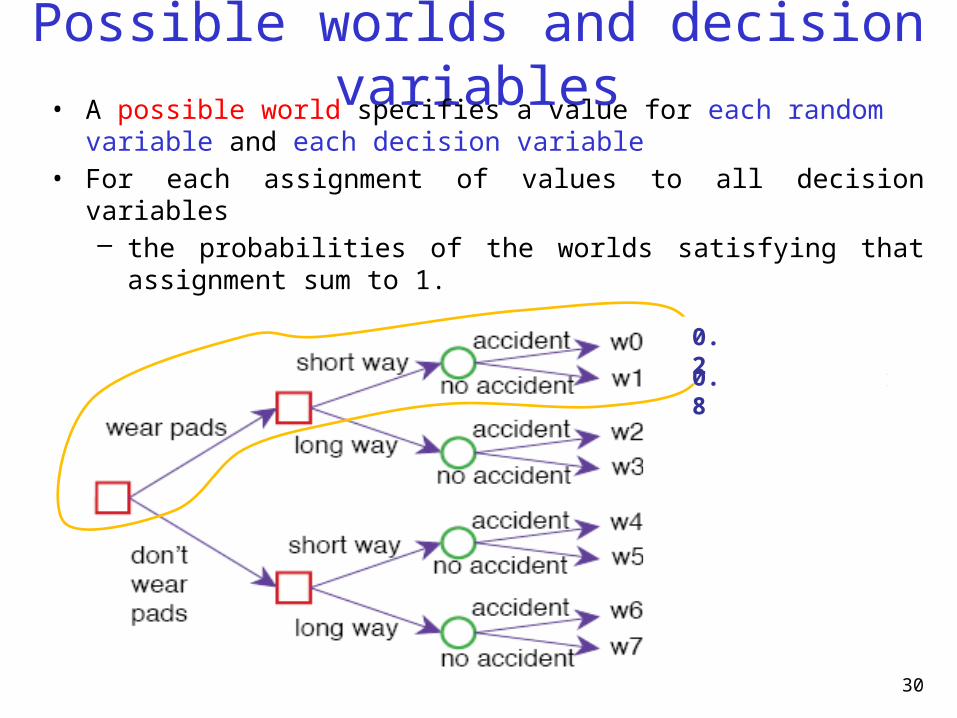
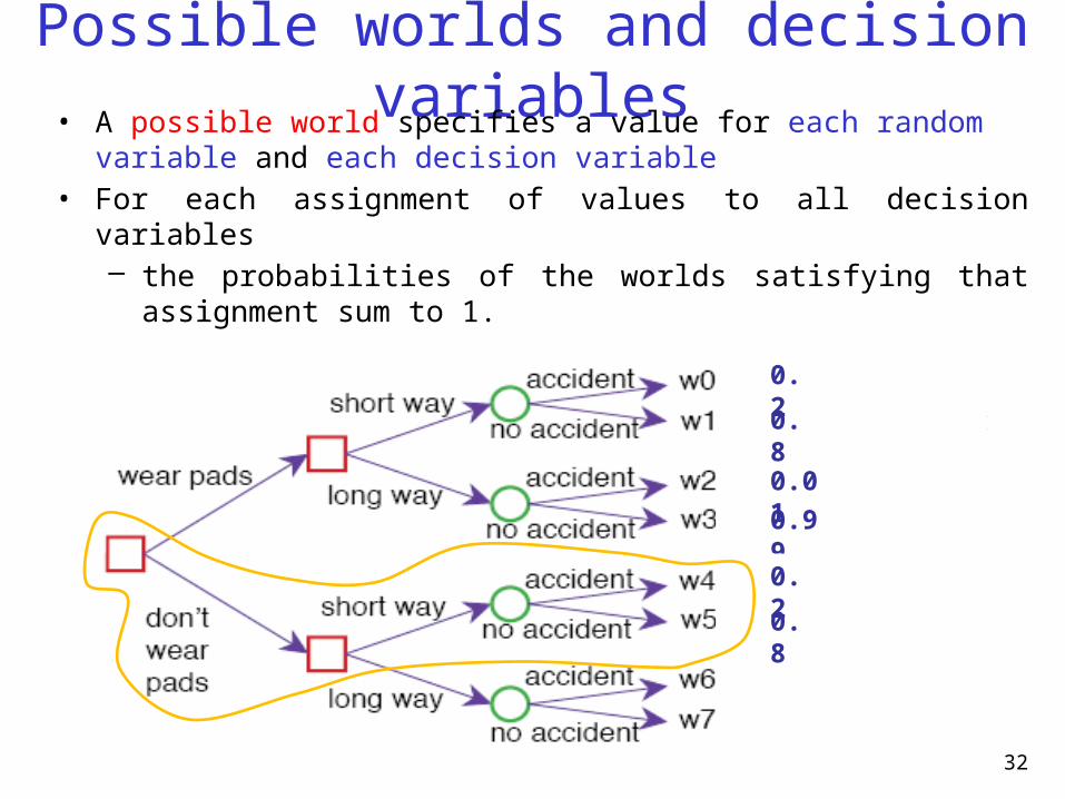
Possible worlds and decision variables• A possible world specifies a value for each random variable and each decision
variable• For each assignment of values to all decision variables
– the probabilities of the worlds satisfying that assignment sum to 1.
0.2
0.8
30
Possible worlds and decision variables
0.01
0.99
0.2
0.8
31
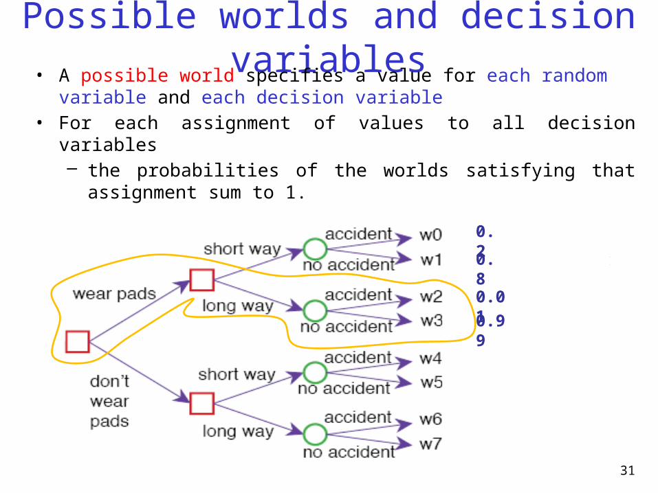
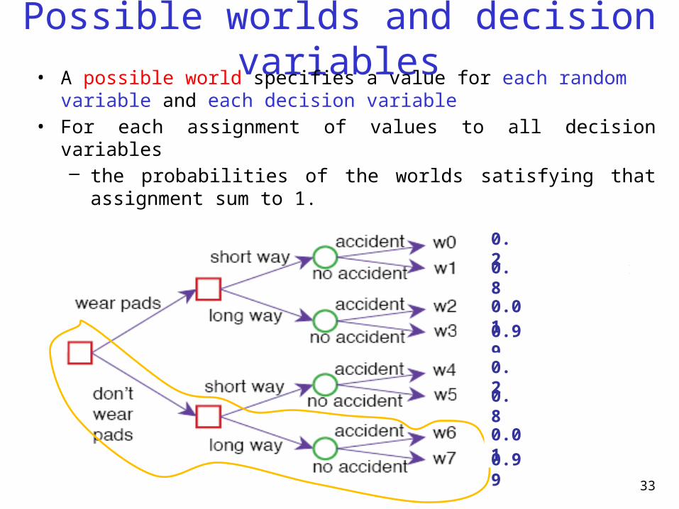
• A possible world specifies a value for each random variable and each decision variable
• For each assignment of values to all decision variables – the probabilities of the worlds satisfying that assignment sum to 1.
Possible worlds and decision variables
0.01
0.99
0.2
0.8
0.2
0.8
32
• A possible world specifies a value for each random variable and each decision variable
• For each assignment of values to all decision variables – the probabilities of the worlds satisfying that assignment sum to 1.
Possible worlds and decision variables
0.01
0.99
0.2
0.8
0.01
0.99
0.2
0.8
33
• A possible world specifies a value for each random variable and each decision variable
• For each assignment of values to all decision variables – the probabilities of the worlds satisfying that assignment sum to 1.
Lecture Overview
• Recap Lecture 11• Decisions under Uncertainty
– Intro– Utility and expected utility
• Single stage decision problems• Decision networks• Sequential Decision Problems
34
Utility• Utility: a measure of desirability of possible worlds to an agent
– Let U be a real-valued function such that U(w) represents an agent's degree of preference for world w
– Expressed by a number in [0,100]
35
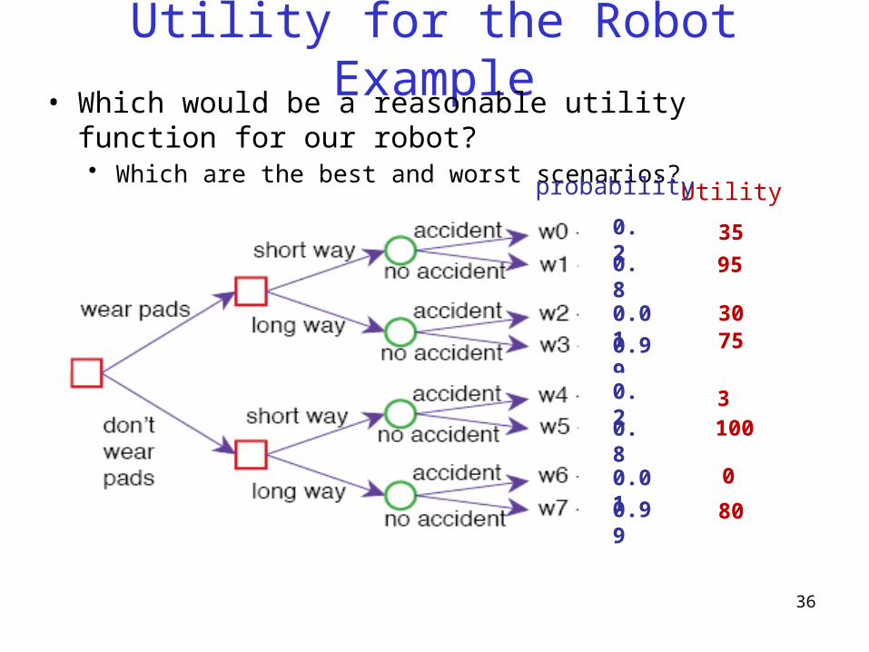
Utility for the Robot Example• Which would be a reasonable utility function for our robot?
• Which are the best and worst scenarios?
0.01
0.99
0.2
0.8
0.01
0.99
0.2
0.8
36
Utilityprobability
35
95
3075
3100
0
80

Utility: Simple Goals– How can the simple (boolean) goal “reach the room” be
specified? B.
A.
C .
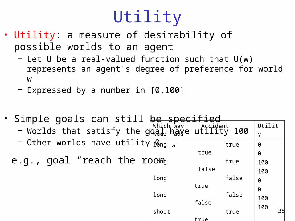
Utility• Utility: a measure of desirability of possible worlds to an agent
– Let U be a real-valued function such that U(w) represents an agent's degree of preference for world w
– Expressed by a number in [0,100]
• Simple goals can still be specified– Worlds that satisfy the goal have utility 100– Other worlds have utility 0
38
Which way Accident Wear Pads
Utility
long true true long true falselong false truelong false falseshort true trueshort true falseshort false trueshort false false
0010010000100100
e.g., goal “reach the room”
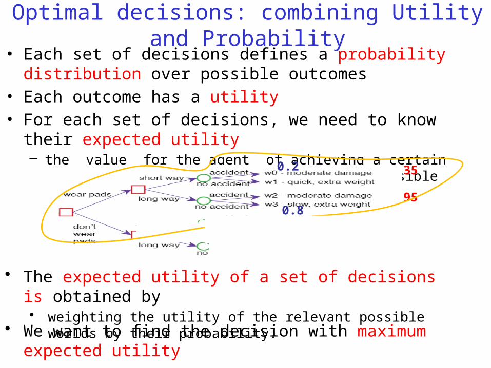
Optimal decisions: combining Utility and Probability• Each set of decisions defines a probability distribution over
possible outcomes• Each outcome has a utility• For each set of decisions, we need to know their expected utility
– the value for the agent of achieving a certain probability distribution over outcomes (possible worlds)
• The expected utility of a set of decisions is obtained by • weighting the utility of the relevant possible worlds by their probability.
35
95
0.2
0.8
• We want to find the decision with maximum expected utility
value of this scenario?
Expected utility of a decision
0.01
0.99
0.2
0.8
0.01
0.99
0.2
0.8
40
Utility
3535
95
probability E[U|D]
3530
75
353
100
350
80
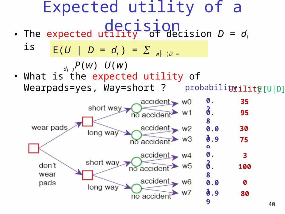
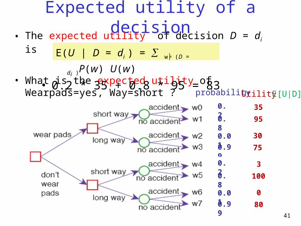
• The expected utility of decision D = di is
• What is the expected utility of Wearpads=yes, Way=short ?
E(U | D = di ) = w╞ (D = di )P(w)
U(w)
Expected utility of a decision
0.01
0.99
0.2
0.8
0.01
0.99
0.2
0.8
41
Utility
3535
95
probability E[U|D]
3530
75
353
100
350
80
• The expected utility of decision D = di is
• What is the expected utility of Wearpads=yes, Way=short ?
E(U | D = di ) = w╞ (D = di )P(w)
U(w)
• 0.2 * 35 + 0.8 * 95 = 83
Expected utility of a decision
0.01
0.99
0.2
0.8
0.01
0.99
0.2
0.8
42
Utility
3535
95
probability E[U|D]
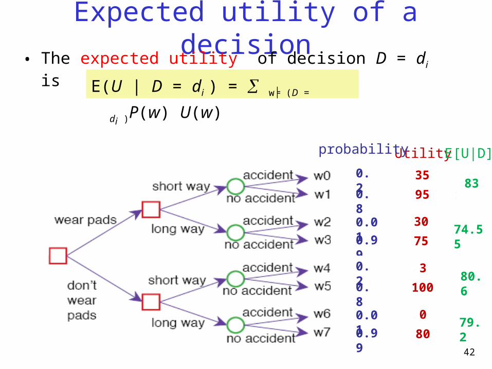
83
3530
75
353
100
350
80
74.55
80.6
79.2
• The expected utility of decision D = di is
E(U | D = di ) = w╞ (D = di )P(w)
U(w)
Lecture Overview
• Recap Lecture 11• Decisions under Uncertainty
– Intro– Utility and expected utility
• Single stage decision problems• Decision networks• Sequential Decision Problems
43
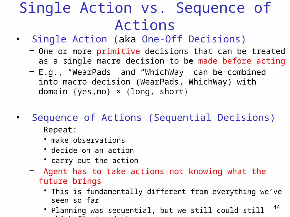
Single Action vs. Sequence of Actions• Single Action (aka One-Off Decisions)
– One or more primitive decisions that can be treated as a single macro decision to be made before acting
– E.g., “WearPads” and “WhichWay” can be combined into macro decision (WearPads, WhichWay) with domain {yes,no} × {long, short}
• Sequence of Actions (Sequential Decisions)– Repeat:
• make observations• decide on an action• carry out the action
– Agent has to take actions not knowing what the future brings• This is fundamentally different from everything we’ve seen so far• Planning was sequential, but we still could still think first and then act
44
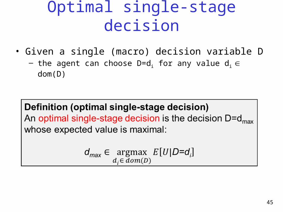
Optimal single-stage decision
• Given a single (macro) decision variable D– the agent can choose D=di for any value di dom(D)
45
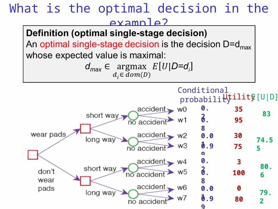
What is the optimal decision in the example?
0.01
0.99
0.2
0.8
0.01
0.99
0.2
0.8
Utility
3535
95
Conditional probability E[U|D]
83
3530
75
353
100
350
80
74.55
80.6
79.2
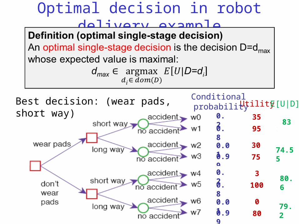
Optimal decision in robot delivery example
0.01
0.99
0.2
0.8
0.01
0.99
0.2
0.8
Utility
3535
95
Conditional probability E[U|D]
83
3530
75
353
100
350
80
74.55
80.6
79.2
Best decision: (wear pads, short way)
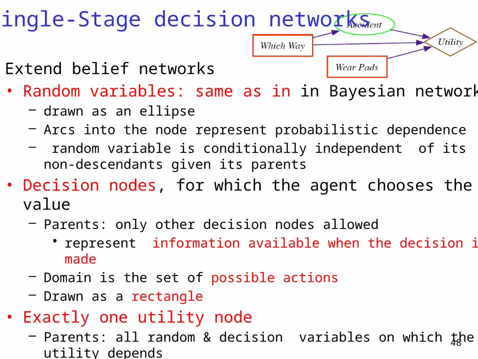
Single-Stage decision networks
Extend belief networks• Random variables: same as in in Bayesian networks
– drawn as an ellipse– Arcs into the node represent probabilistic dependence– random variable is conditionally independent of its non-descendants given its
parents
• Decision nodes, for which the agent chooses the value– Parents: only other decision nodes allowed
• represent information available when the decision is made– Domain is the set of possible actions – Drawn as a rectangle
• Exactly one utility node– Parents: all random & decision variables on which the utility depends– Specifies a utility for each instantiation of its parents– Drawn as a diamond 48
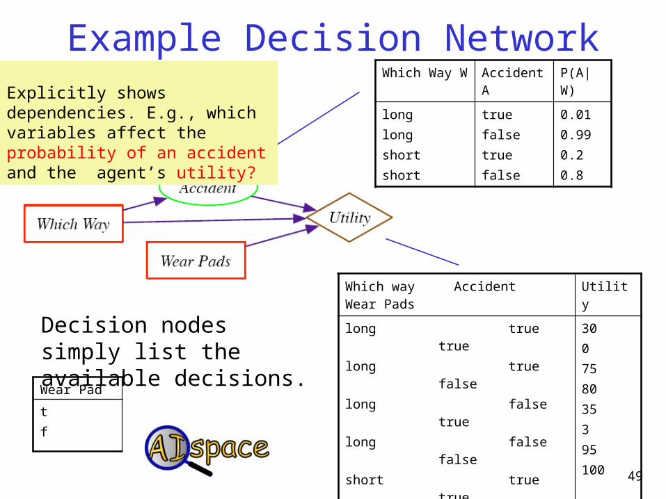
Example Decision Network
Decision nodes simply list the available decisions.
49
Which way Accident Wear Pads
Utility
long true true long true falselong false truelong false falseshort true trueshort true falseshort false trueshort false false
300 75 8035395 100
Which Way W
Accident A
P(A|W)
longlong shortshort
true false true false
0.01 0.99 0.2 0.8
Explicitly shows dependencies. E.g., which variables affect the probability of an accident and the agent’s utility?
Wear Pad
tf
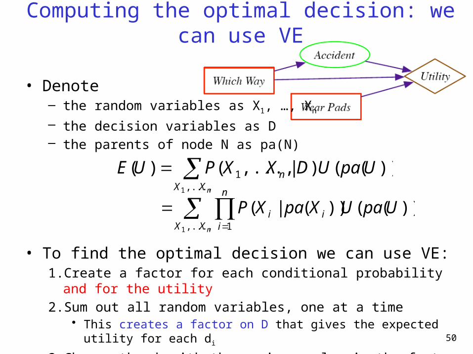
Computing the optimal decision: we can use VE
• Denote– the random variables as X1, …, Xn
– the decision variables as D– the parents of node N as pa(N)
• To find the optimal decision we can use VE:1. Create a factor for each conditional probability and for the utility
2. Sum out all random variables, one at a time• This creates a factor on D that gives the expected utility for each di
3. Choose the di with the maximum value in the factor
nXX
n UpaUDXXPUE,...,
1
1
))(()|,...,()(
nXX
n
iii UpaUXpaXP
,..., 11
))(())(|(
50
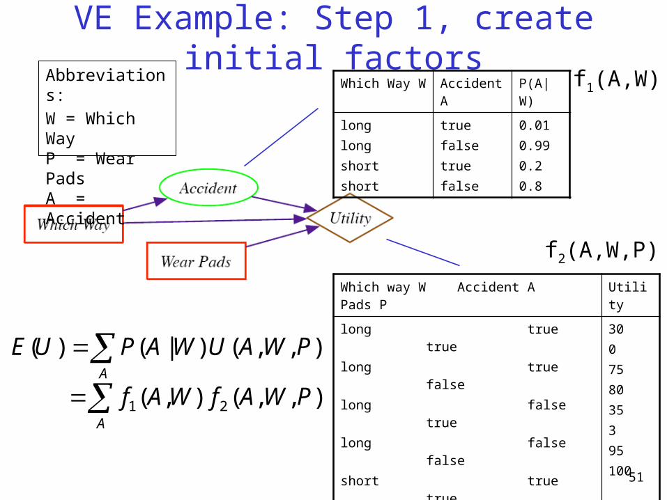
VE Example: Step 1, create initial factors
51
Which way W Accident A Pads P Utility
long true true long true falselong false truelong false falseshort true trueshort true falseshort false trueshort false false
300 75 8035395 100
Which Way W
Accident A
P(A|W)
longlong shortshort
true false true false
0.01 0.99 0.2 0.8
f1(A,W)
f2(A,W,P)
A
PWAUWAPUE ),,()|()(
A
PWAfWAf ),,(),( 21
Abbreviations:
W = Which WayP = Wear PadsA = Accident
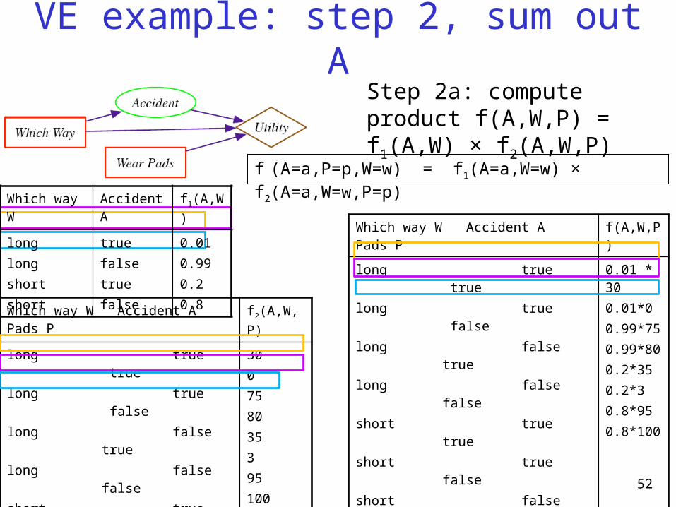
Which way W Accident A Pads P f(A,W,P)
long true true long true falselong false truelong false falseshort true trueshort true falseshort false trueshort false false
0.01 * 300.01*00.99*750.99*800.2*350.2*30.8*95 0.8*100
VE example: step 2, sum out AStep 2a: compute product f(A,W,P) = f1(A,W) × f2(A,W,P)
52
Which way W Accident A Pads P
f2(A,W,P)
long true true long true falselong false truelong false falseshort true trueshort true falseshort false trueshort false false
300 75 8035395 100
f (A=a,P=p,W=w) = f1(A=a,W=w) × f2(A=a,W=w,P=p)Which way
WAccident A
f1(A,W)
longlong shortshort
true false true false
0.01 0.99 0.2 0.8
VE example: step 2, sum out A
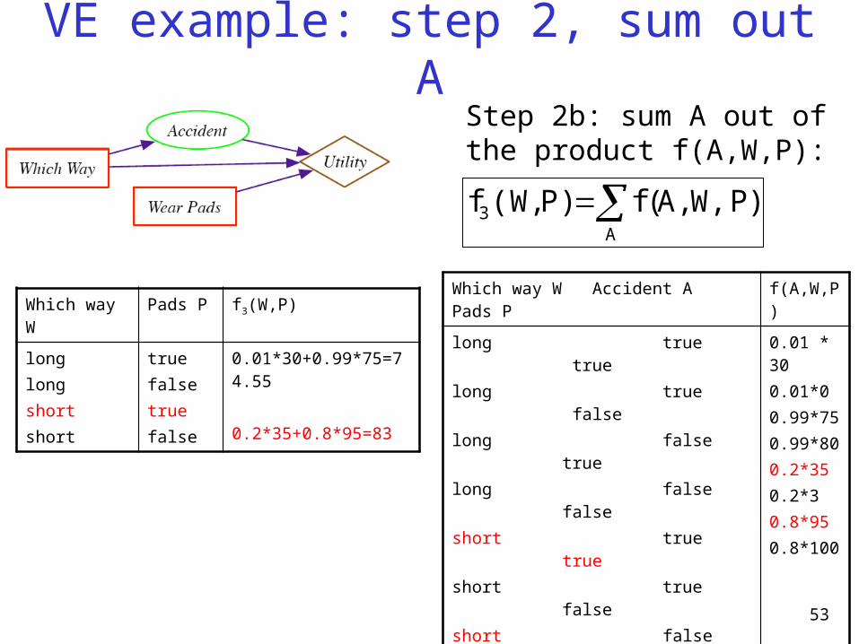
53
Which way W
Pads P f3(W,P)
longlong shortshort
true false true false
0.01*30+0.99*75=74.55
0.2*35+0.8*95=83
Which way W Accident A Pads P f(A,W,P)
long true true long true falselong false truelong false falseshort true trueshort true falseshort false trueshort false false
0.01 * 300.01*00.99*750.99*800.2*350.2*30.8*95 0.8*100
Step 2b: sum A out of the product f(A,W,P):
A3 )PW,A,(f P)(W,f
VE example: step 2, sum out A
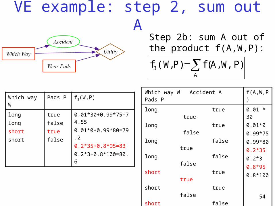
54
Which way W
Pads P f3(W,P)
longlong shortshort
true false true false
0.01*30+0.99*75=74.550.01*0+0.99*80=79.20.2*35+0.8*95=830.2*3+0.8*100=80.6
Which way W Accident A Pads P f(A,W,P)
long true true long true falselong false truelong false falseshort true trueshort true falseshort false trueshort false false
0.01 * 300.01*00.99*750.99*800.2*350.2*30.8*95 0.8*100
Step 2b: sum A out of the product f(A,W,P):
A3 )PW,A,(f P)(W,f
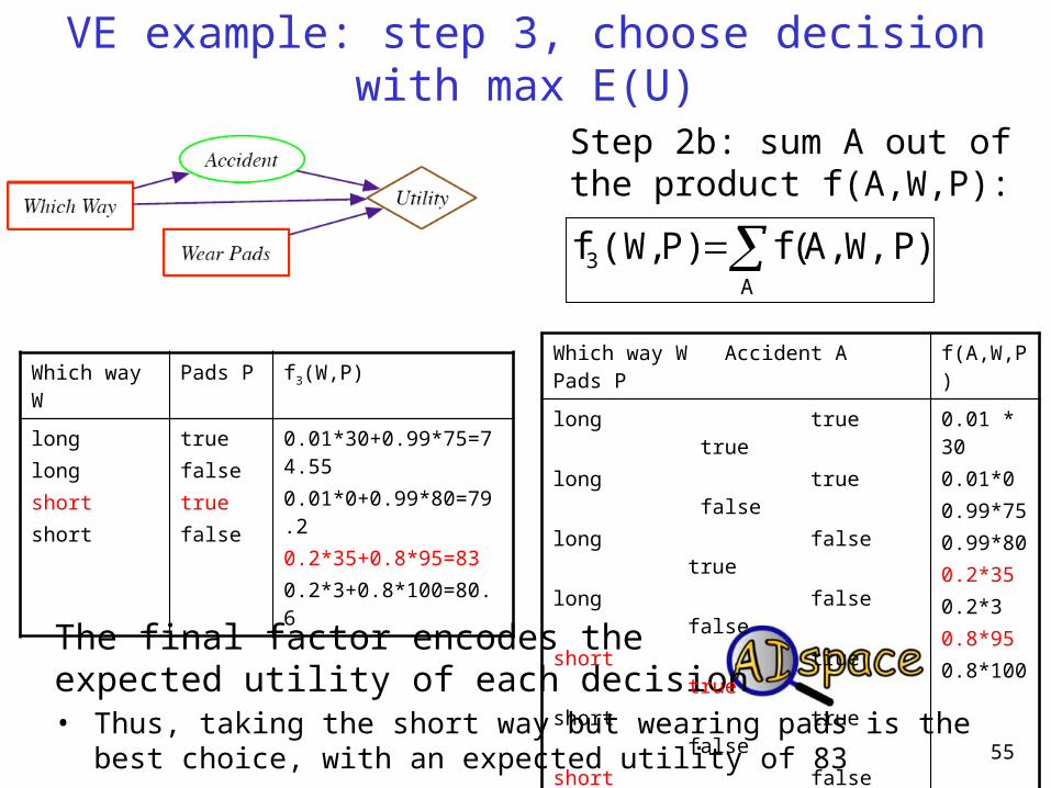
The final factor encodes the expected utility of each decision• Thus, taking the short way but wearing pads is the best choice, with an
expected utility of 83
VE example: step 3, choose decision with max E(U)
55
Which way W
Pads P f3(W,P)
longlong shortshort
true false true false
0.01*30+0.99*75=74.550.01*0+0.99*80=79.20.2*35+0.8*95=830.2*3+0.8*100=80.6
Which way W Accident A Pads P f(A,W,P)
long true true long true falselong false truelong false falseshort true trueshort true falseshort false trueshort false false
0.01 * 300.01*00.99*750.99*800.2*350.2*30.8*95 0.8*100
Step 2b: sum A out of the product f(A,W,P):
A3 )PW,A,(f P)(W,f
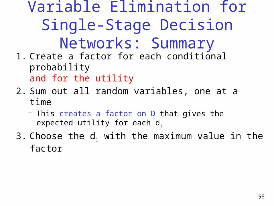
Variable Elimination for Single-Stage Decision Networks: Summary
1. Create a factor for each conditional probability and for the utility
2. Sum out all random variables, one at a time– This creates a factor on D that gives the expected utility for each di
3. Choose the di with the maximum value in the factor
56