Embed Size (px)
Citation preview

Decision making as a model
4. Signal detection: models and measures

1. Hard workGet several points on ROC-curve by inducing several criteria (pay-off, signal frequency)
Compute hit rate and false alarm rate at every criterion Many trials for every point!
Measure or compute A using graphical methods
Nice theorems, but how to proceed in practice?

Certainly 0 1 2 3 4 5 Certainlyno signal a signal
Variant: numeric (un)certainty scale: implies multiple criteria – consumes many trials too
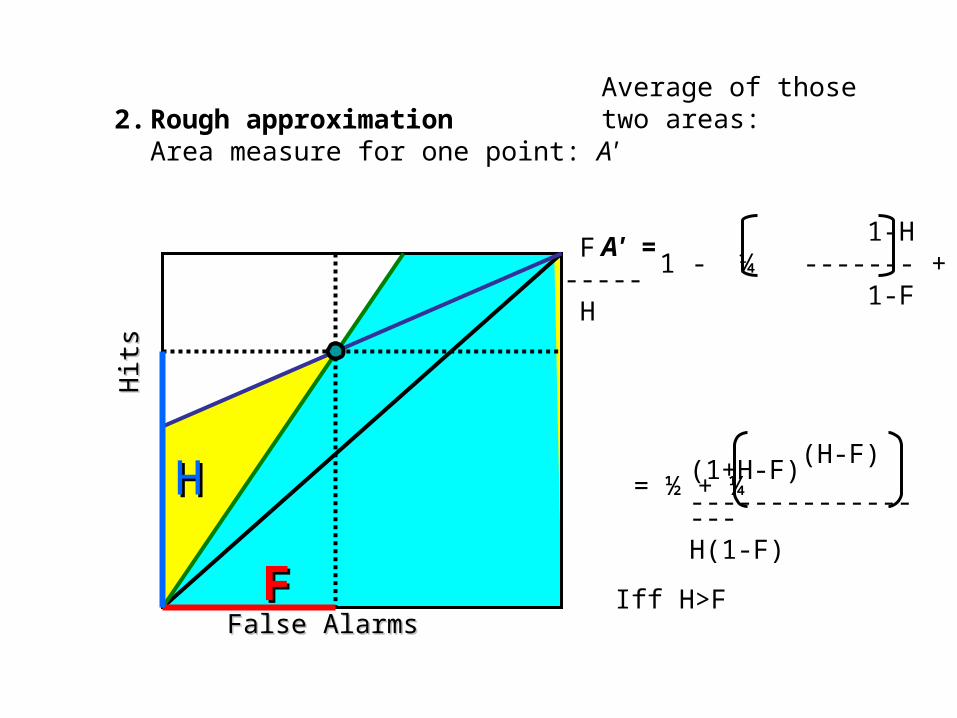
2. Rough approximationArea measure for one point: A'
Hits
Hits
False AlarmsFalse AlarmsFF
HH
Average of those two areas:
A' = 1-H F1 - ¼ ------- + ----- 1-F H
(H-F)(1+H-F)= ½ + ¼ -----------------
H(1-F)
Iff H>F

Comparable measure for criterion/bias: Grier’s B''
H(1 - H) – F(1 – F) B'' = sign(H - F) ------------------------ H(1 - H) + F(1 – F)
if H = 1 - F then B'' = 0
if F = 0, H≠ 0, H≠1 then B'' = 1
if H = 1, F≠0, F≠1, then B'' = -1
HH
FF
FALSE ALARM RATE
HIT
RA
TE
B''= -.4
B''= -.07
B''=
.0
7
B''=
.4
B''= 0
Isobias curves

3. Introducing assumptions
Even when several points ara available, they may not lie on a nice curve
Then you might fit a curve, but which one?
Every curve reflects some (implicit) assumptions about distributions
Save labor: more assumptions less measurement(but the assumptions may not be justified)

Simplest model:
noise and signal distributions normal with equal variance
One point (PH, PFA pair) is sufficient
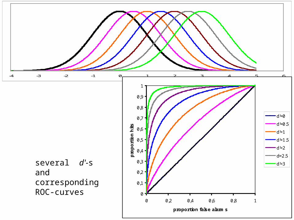
Normal distributions are popular (there are other models!)
0
0,05
0,1
0,15
0,2
0,25
0,3
0,35
0,4
0,45
-4 -3 -2 -1 0 1 2 3 4 5

Example: in an experiment with noise trials and signal trials these results were obtained:
Hit rate: .933, False Alarm rate .309(.067 misses and .691 correct rejections)
Normal distributions: via corresponding z-scores the complete model can be reconstructed:

z.309 = .5
z.933 = - 1.5
distance: d´ = 2 measure for “sensitivity”
.933
.309.309
hf
hβ = ---- = .37 fMeasure forbias/criterion
-4 -3 -2 -1 0 1 2 3 4 5 6
0
0,1
0,2
0,3
0,4
0,5
0,6
0,7
0,8
0,9
1
0 0,2 0,4 0,6 0,8 1
proportion false alarms
pro
po
rtio
n h
its
d'=0
d'=0.5
d'=1
d'=1.5
d'=2
d=2.5
d'=3several d'-s and corresponding ROC-curves

Gaussian models: preliminary
Standaard normal curveM=0, sd = 1
Transformations:
Φ(z) P
Φ-1(P) or: Z(P) z see tabels and standard software
1 φ(z)= e-z2/2 √2π
z Φ(z) = -∞ φdx
∫z
P

PH
PFA
zH
zFA
Roc-curve PH = f(PFA)
Z-transformation ROC-curve
P z zH = f(zFA)
λλ
Nice way to plot several (PFA, PH) points
-

Regression line
zH = a1zFA+ b1,
Minimize (squared) deviations zH : Underestimation of a
Compromise: average of regression lines
ZH = ½(a1+1/a2)ZFA + ½(b1+b2/a2)
Plotting with regression line?
Regresionline
zFA= a2zH + b2
Minimize (squared) deviations zFA : Overestimation of a

zH
zFA
d'
Equal variance model:
zH = zFA + d' d' = zH –zFA
z-plot ROC 45°
PFA = 1- Φ(λ), = Φ(-λ), zFA = -λ
PH = 1 – Φ(-(d' - λ)) = Φ(d' – λ), zH = d' – λ
d'45°
0 λ

ff
β = h/f = φ(zH)/φ(zF)
To get symmety a log transformation is often applied:
log β = log h – log f = ½(z2FA – z2
H )
Criterion/bias:
hh1 -z2/2
φ(z) = ------ e (standard-normal) √(2π)
1 -zH2/2
φ(zH) = ------ e √(2π)
1 -zFA2/2
φ(zFA) = ------ e √(2π)
zFA2 – zH
2
------------ 2
Divide: -------------------- = e

ffhh
λ c
zH + zFA c = - ----------
2
Alternatve: c (aka λcenter),
distance (in sd) between middle (were h=f) and criterion
c = -(d'/2 – λ)
zFA = -λ
d' = zH - zFA
zH – zFA 2zFA c = - ---------- + ----- 2 2

β c
Isobias curves for β en c