Embed Size (px)
Citation preview
Journal of Development Economics 76 (2005) 481–501
www.elsevier.com/locate/econbase
Decentralization and macroeconomic performance in
China: regional autonomy has its costs
Andrew Feltensteina,*, Shigeru Iwatab,1
aInternational Monetary Fund, 700 19th St. NW, Washington, DC 20431, United StatesbDepartment of Economics, University of Kansas, 226L Summerfield Hall, Lawrence, KS 66045, United States
Received 1 May 2002; accepted 1 January 2004
Abstract
We give an empirical examination of the impact of fiscal and economic decentralization in China
on the country’s economic growth and inflation, using a vector autoregressive (VAR) model with
latent variables. Our econometric investigation offers strong evidence that there is a connection
between decentralization and macroeconomic performance in China. Economic decentralization
appears to be positively related to growth in real output for the entire postwar period in China.
Fiscal decentralization seems to have adverse implications for the rate of inflation, especially after
the late 1970s. Decentralization would therefore seem to be good for growth and bad for price
stability.
D 2004 Elsevier B.V. All rights reserved.
JEL classification: E31; H21; O53
Keywords: Fiscal; Decentralization; Stability; China
1. Introduction
This paper investigates empirically whether decentralization in China has been
beneficial for growth and inflation. Decentralization, whether in the form of fiscal
0304-3878/$ -
doi:10.1016/j.
* Corresp
E-mail add1 Tel.: +1
see front matter D 2004 Elsevier B.V. All rights reserved.
jdeveco.2004.01.004
onding author. Tel.: +1 202 6239437; fax: +1 202 623 6440.
resses: [email protected] (A. Feltenstein)8 [email protected] (S. Iwata).
785 8642867.
A. Feltenstein, S. Iwata / Journal of Development Economics 76 (2005) 481–501482
federalism, or in the form of reduced government interference in the private sector, is
generally thought to help an emerging economy. Although the devolution of economic
power has been a central element in the reform process of many transition economies,
there is relatively little empirical work examining the relationship between such
decentralization and changes in the macroeconomy.
Decentralization may improve allocative efficiency, but it may also make stabilization
policies more difficult to carry out. See, e.g., Prudhomme (1994) and Tanzi (1995). China
has instituted rapid economic decentralization, and has simultaneously experienced both
growth and instability. There is a growing consensus in the academic literature about the
mechanisms that create the links between decentralization and economic growth and
inflation in post-reform China (Brandt and Zhu, 2000; Jin et al., 1999; Lardy, 1998;
Naughton, 1995; Yusuf, 1994). A simplified version of such a mechanism may be described
as follows.
Although the aggregate effective tax burden may not have changed, fiscal
decentralization has caused tax revenues to shift from the central government to
regional governments. The regional governments, infused with new revenue,
begin to build local infrastructure. This infrastructure encourages investment, both
of the non-state as well as the state-owned enterprises (SOEs). The non-state
firms tend to respond to the increased local infrastructure with higher rates of
investment than the SOEs, given their greater efficiency. As the SOEs attempt
to keep up with the rates of investment of non-state firms, a further adjustment
occurs. The SOEs, observing the increased rate of capital formation of the non-
state sector, increase their own rate of investment beyond the rate that would
be optimal. The SOEs are able to do so because they have access to local
bank loans that are not justified on economic grounds. This access to the
banking system thereby distinguishes them from the non-state firms.2 The banks
that passively grant these loans are themselves financed by discount lending by the
People’s Bank. The resulting monetary expansion leads to increased inflation, while the
higher output of both the SOEs and non-state enterprises cause an increase in aggregate
real income.
In this paper, we provide a formal empirical examination of decentralization in Chinese
economy, based on published data. We find that (i) decentralization plays indeed a fairly
important role in a VARmodel of growth and inflation, (ii) the pattern of the relation does not
appear to be restricted to the post-reform period, but rather characterizes the entire postwar
economy in China.
The next section will review China’s experiences with decentralization. Section 3 will
discuss our data set, including construction of measures of decentralization. Section 4 will
develop our econometric models, while Section 5 reports the results of estimation and tests
2 This access to local bank loans is a facet of the bsoft budget constraintQ that is a key feature of many
transition economies (see Maskin 1999 and Qian and Xu 1998 for recent theoretical work on the topic). One
might claim that a key distinction between SOEs in China and in a country such as, e.g., Brazil is that the
Brazilian banking system does not lend to the SOEs with the same degree of passivity as does the Chinese
banking system.
A. Feltenstein, S. Iwata / Journal of Development Economics 76 (2005) 481–501 483
that have been carried out with those models. The final section is a summary and
conclusion.
2. Background
2.1. Decentralization in China
Between 1949 and 2001, the Chinese economy experienced frequent cycles, with
economic policy shifting between decentralization and recentralization programs. In the
early 1950s, the Soviet model of central planning shaped the relationships between the
State Council and local governments. The central authority exercised direct administrative
control over local governments through three central planning mechanisms: the physical
planning of production, centralized allocation of materials, and budgetary control of
revenues and expenditures.
Concentration of power at the center reduced the initiative of local governments
and hindered production, leading, in 1957, to the move to decentralization. A wave of
recentralization, however, began in the early 1960s, when almost all large and
medium-sized enterprises were returned to the central authority. A new decentral-
ization movement started in 1964 and continued throughout the Cultural Revolution
period.
Before 1979, China’s budgetary policy essentially consisted in generalized tax
collection and profit remittances controlled by the central government and then
redistributed as needed to the provinces. This system of beating from one potQ was
changed in the 1980 intergovernmental reform, under which different jurisdictions were
assigned different expenditure responsibilities and were also made responsible for
collecting necessary revenues.
Chinese fiscal decentralization has had certain features relevant to our study.3 China has
never had a true central tax administration. All taxes, with the exception of excises, have
been collected by local governments and then shared with the central government.
Accordingly, as decentralization has progressed, local governments that wish to promote
growth have tended to reduce their tax effort and revenue sharing with the central
government. This has resulted in the stagnation of revenue from indirect taxes despite
rapid growth in the economy.
2.2. Growth and inflation
2.2.1. Pre-reform period
The Chinese economy in the pre-reform period has been characterized by a cycle of
policy shifts, or bstop and goQ economic programs. Decentralization programs, intended to
3 For a review of Chinese fiscal decentralization, see Bell et al. (1993), Lardy (1998), Tseng et al. (1994),
Hofman (1993), World Bank (1994, 1996) and G. Ma (1995). A broad historical, as well as analytical, survey of
Chinese fiscal and macroeconomic policies is given in J. Ma (1997).
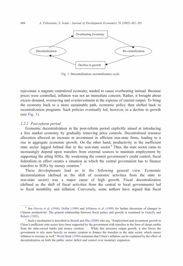
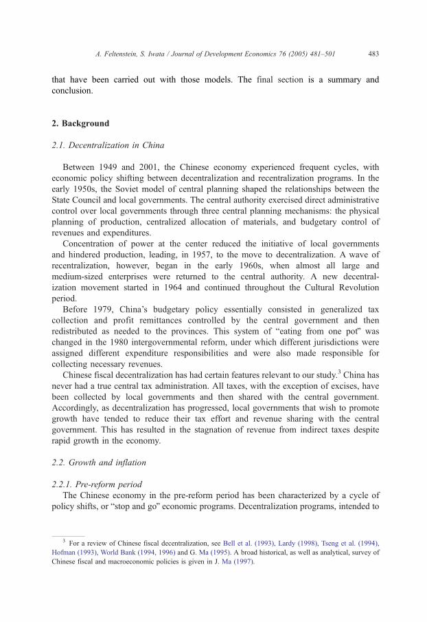
Fig. 1. Decentralization–recentralization cycle.
A. Feltenstein, S. Iwata / Journal of Development Economics 76 (2005) 481–501484
rejuvenate a stagnate centralized economy, tended to cause overheating instead. Because
prices were controlled, inflation was not an immediate concern. Rather, it brought about
excess demand, oversaving and overinvestment at the expense of current output. To bring
the economy back to a more sustainable path, economic policy then shifted back to
recentralization programs. Such policies eventually led, however, to a decline in growth
(see Fig. 1).
2.2.2. Post-reform period
Economic decentralization in the post-reform period explicitly aimed at introducing
a free market economy by gradually removing price controls. Decentralized resource
allocation allowed an increase in investment in efficient non-state firms, leading to a
rise in aggregate economic growth. On the other hand, productivity in the inefficient
state sector lagged behind that in the non-state sector.4 Thus, the state sector came to
increasingly depend upon transfers from external sources to maintain employment by
supporting the ailing SOEs. By weakening the central government’s credit control, fiscal
federalism in effect creates a situation in which the central government has to finance
transfers to SOEs by money creation.5
These developments lead us to the following general view. Economic
decentralization (defined as the shift of economic activities from the state to
non-state sector) was a major cause of high growth. Fiscal decentralization
(defined as the shift of fiscal activities from the central to local governments) led
to fiscal instability and inflation. Conversely, some authors have argued that fiscal
4 See Groves et al. (1994), Dollar (1990) and Jefferson et al. (1999) for further discussion of changes in
Chinese productivity. The general relationship between fiscal policy and growth is examined in Easterly and
Rebelo (1993).5 Such a mechanism is described in Brandt and Zhu (2000) who say, bEmployment and investment growth in
China’s inefficient state sector have been supported by the government with transfers in the form of cheap credits
from the state-owned banks and money creation. . . . While this increases output growth, it also forces the
government to rely more heavily on money creation to finance the transfers to the state sector, which causes
inflation to increase as well.QWorld Bank (1994) maintains that China’s inflation can be explained by the effect of
decentralization on both the public sector deficit and control over monetary expansion.
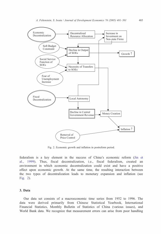
Fig. 2. Economic growth and inflation in postreform period.
A. Feltenstein, S. Iwata / Journal of Development Economics 76 (2005) 481–501 485
federalism is a key element in the success of China’s economic reform (Jin et
al., 1999). Thus, fiscal decentralization, i.e., fiscal federalism, created an
environment in which economic decentralization could exist and have a positive
effect upon economic growth. At the same time, the resulting interaction between
the two types of decentralization leads to monetary expansion and inflation (see
Fig. 2).
3. Data
Our data set consists of a macroeconomic time series from 1952 to 1996. The
data were derived primarily from Chinese Statistical Yearbook, International
Financial Statistics, Monthly Bulletin of Statistics of China (various issues), and
World Bank data. We recognize that measurement errors can arise from poor handling
A. Feltenstein, S. Iwata / Journal of Development Economics 76 (2005) 481–501486
of data and distortions by government bureaucrats. It is also possible that some
observed variables in China do not reflect properly economic activity. In earlier
periods, prices were not market determined but controlled by the central government.
Nonetheless, we treat the data as if there were no serious problems in its quality and
relevance. We do so because we believe that doing so is a useful route to take, at least for a
first trial.6
3.1. GNP and price series
The two basic series for our study are the Chinese real gross national product (GNP)
and the retail price index.7 The series, for the period 1952–1996 are displayed in Fig. 3A,
while their first differences, GNP growth and the inflation rate, are shown in Fig. 3B.
An upward trend in real GNP is interrupted twice by sharp declines in 1961 and 1968
(Fig. 3A). The first drop is about a 35% decline from the previous year, the period
known as the bGreat FamineQ (1959–1961), an outcome of the economic and social
programs of the bGreat Leap Forward.Q The second drop, of about 10%, occurred in
the early part of the Cultural Revolution (1966–1976). The rate of inflation during the
entire 10 years period of the Cultural Revolution was virtually zero (Fig. 3B), a result of
extremely tight price controls. While GNP growth and inflation do not appear to be
correlated over the full period 1952–1996, they do after the initiation of the economic
reform in 1979. The simple correlation is 0.33 for 1952–1996, but this conceals a sharp
contrast between the pre- and post-reform period. The correlation is �0.59 for the
period 1952–1978, while it is 0.71 for the period 1979–1996. This striking change is
consistent with the point mentioned in Section 2.2.2 and emphasized by Brandt and Zhu
(2000).
Table 1 provides the Dickey–Fuller test for GNP and price series. Based on a regression
of growth on a constant, lagged log of GNP, and 2–4 lags of growth, the test t(b) of the unitroot (i.e., b=0) for GNP given no drift (a=0) cannot be rejected. The F-test of a=b=0 is,
however, rejected. Then we test a=0, given that there is a unit root, and find it rejected [t(a)].
7 More precisely, our output series is the national income of the material product system, rather than GNP, as
published data of the latter began in 1978.
6 We treat the data as if there are no measurement errors, not because we have some reasons to believe the
measurement errors are entirely insignificant, but because a careless attempt to correct the data would frequently
make a situationworse and because even biased estimates often carry useful information. For example, some authors
suspect that official data overstate growth and understate inflation during the reform period (Lardy, 1998, Feltenstein
and Ha, 1991, Feltenstein et al., 1990). World Bank (1997) even provides estimates of the size of errors—
overstatement of the rate of growth by about 1.3 percentage points a year for 1986–1995. We experimentally re-
estimated our VAR model with the error corrected data based on the size of errors suggested by World Bank. The
results (not shown) are not importantly different from those reported in Section 5. On the other hand, the relevancy
of the measured variables, e.g., that of the measured price variable under price controls, is to some extent an
empirically testable proposition. We examined whether the price variable plays a qualitatively different role in our
VAR model between the period of the tight price control and the post reform period. When the Cultural Revolution
dummy (1966–1976) was included in the VAR, we found the dummy to not be significant, and there were no
changes in other parameter estimates. Hence, the price controls appear not to have been very important in our VAR
model.
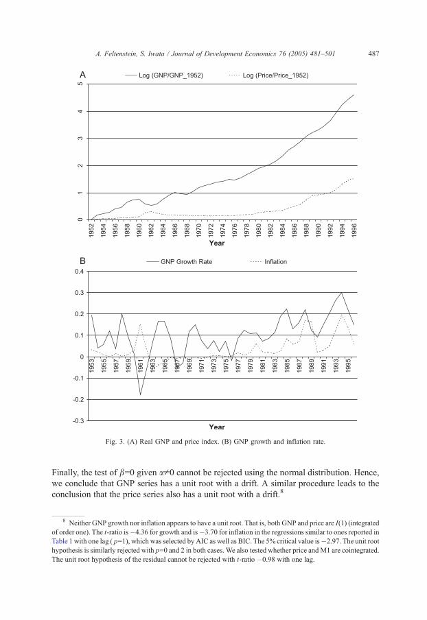
Fig. 3. (A) Real GNP and price index. (B) GNP growth and inflation rate.
A. Feltenstein, S. Iwata / Journal of Development Economics 76 (2005) 481–501 487
Finally, the test of b=0 given ap0 cannot be rejected using the normal distribution. Hence,
we conclude that GNP series has a unit root with a drift. A similar procedure leads to the
conclusion that the price series also has a unit root with a drift.8
8 Neither GNP growth nor inflation appears to have a unit root. That is, both GNP and price are I(1) (integrated
of order one). The t-ratio is�4.36 for growth and is�3.70 for inflation in the regressions similar to ones reported in
Table 1 with one lag ( p=1), which was selected by AIC as well as BIC. The 5% critical value is�2.97. The unit root
hypothesis is similarly rejected with p=0 and 2 in both cases. We also tested whether price and M1 are cointegrated.
The unit root hypothesis of the residual cannot be rejected with t-ratio �0.98 with one lag.
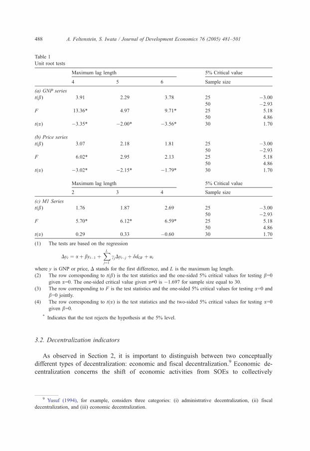
Table 1
Unit root tests
Maximum lag length 5% Critical value
4 5 6 Sample size
(a) GNP series
t(b) 3.91 2.29 3.78 25 �3.00
50 �2.93
F 13.36* 4.97 9.71* 25 5.18
50 4.86
t(a) �3.35* �2.00* �3.56* 30 1.70
(b) Price series
t(b) 3.07 2.18 1.81 25 �3.00
50 �2.93
F 6.02* 2.95 2.13 25 5.18
50 4.86
t(a) �3.02* �2.15* �1.79* 30 1.70
Maximum lag length 5% Critical value
2 3 4 Sample size
(c) M1 Series
t(b) 1.76 1.87 2.69 25 �3.00
50 �2.93
F 5.70* 6.12* 6.59* 25 5.18
50 4.86
t(a) 0.29 0.33 �0.60 30 1.70
(1) The tests are based on the regression
Dyt ¼ a þ byt�1 þXLj¼1
cjDyt�j þ ddGF þ ut
where y is GNP or price, D stands for the first difference, and L is the maximum lag length.
(2) The row corresponding to t(b) is the test statistics and the one-sided 5% critical values for testing b=0given a=0. The one-sided critical value given ap0 is �1.697 for sample size equal to 30.
(3) The row corresponding to F is the test statistics and the one-sided 5% critical values for testing a=0 and
b=0 jointly.
(4) The row corresponding to t(a) is the test statistics and the two-sided 5% critical values for testing a=0given b=0.
* Indicates that the test rejects the hypothesis at the 5% level.
A. Feltenstein, S. Iwata / Journal of Development Economics 76 (2005) 481–501488
3.2. Decentralization indicators
As observed in Section 2, it is important to distinguish between two conceptually
different types of decentralization: economic and fiscal decentralization.9 Economic de-
centralization concerns the shift of economic activities from SOEs to collectively
9 Yusuf (1994), for example, considers three categories: (i) administrative decentralization, (ii) fiscal
decentralization, and (iii) economic decentralization.
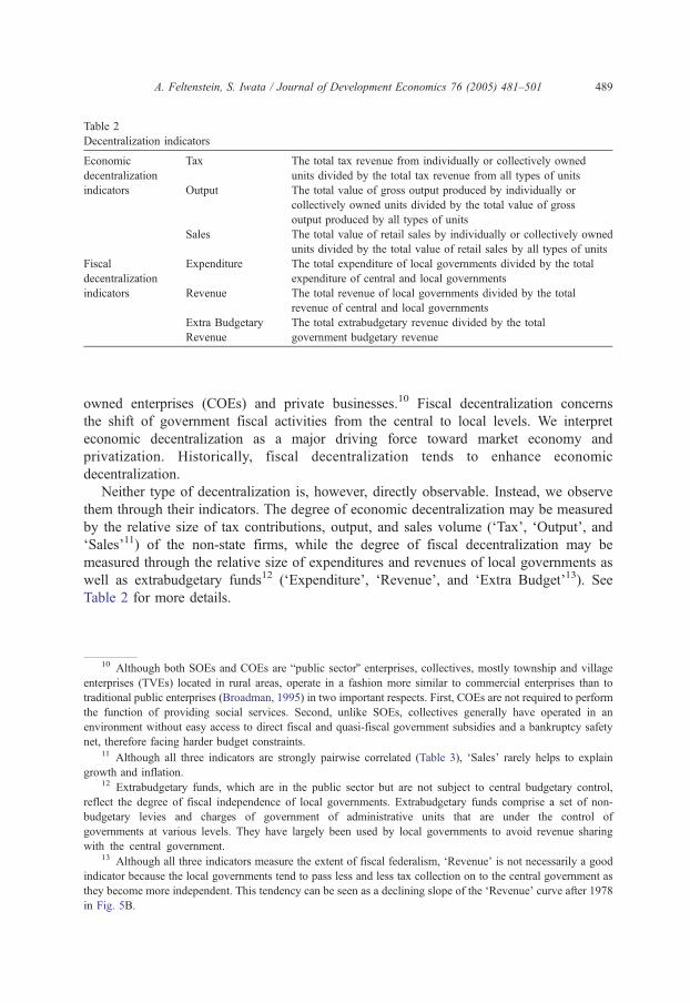
Table 2
Decentralization indicators
Economic
decentralization
indicators
Tax The total tax revenue from individually or collectively owned
units divided by the total tax revenue from all types of units
Output The total value of gross output produced by individually or
collectively owned units divided by the total value of gross
output produced by all types of units
Sales The total value of retail sales by individually or collectively owned
units divided by the total value of retail sales by all types of units
Fiscal
decentralization
indicators
Expenditure The total expenditure of local governments divided by the total
expenditure of central and local governments
Revenue The total revenue of local governments divided by the total
revenue of central and local governments
Extra Budgetary
Revenue
The total extrabudgetary revenue divided by the total
government budgetary revenue
A. Feltenstein, S. Iwata / Journal of Development Economics 76 (2005) 481–501 489
owned enterprises (COEs) and private businesses.10 Fiscal decentralization concerns
the shift of government fiscal activities from the central to local levels. We interpret
economic decentralization as a major driving force toward market economy and
privatization. Historically, fiscal decentralization tends to enhance economic
decentralization.
Neither type of decentralization is, however, directly observable. Instead, we observe
them through their indicators. The degree of economic decentralization may be measured
by the relative size of tax contributions, output, and sales volume (dTaxT, dOutputT, anddSalesT11) of the non-state firms, while the degree of fiscal decentralization may be
measured through the relative size of expenditures and revenues of local governments as
well as extrabudgetary funds12 (dExpenditureT, dRevenueT, and dExtra BudgetT13). SeeTable 2 for more details.
11 Although all three indicators are strongly pairwise correlated (Table 3), dSalesT rarely helps to explain
growth and inflation.12 Extrabudgetary funds, which are in the public sector but are not subject to central budgetary control,
reflect the degree of fiscal independence of local governments. Extrabudgetary funds comprise a set of non-
budgetary levies and charges of government of administrative units that are under the control of
governments at various levels. They have largely been used by local governments to avoid revenue sharing
with the central government.13 Although all three indicators measure the extent of fiscal federalism, dRevenueT is not necessarily a good
indicator because the local governments tend to pass less and less tax collection on to the central government as
they become more independent. This tendency can be seen as a declining slope of the dRevenueT curve after 1978in Fig. 5B.
10 Although both SOEs and COEs are bpublic sectorQ enterprises, collectives, mostly township and village
enterprises (TVEs) located in rural areas, operate in a fashion more similar to commercial enterprises than to
traditional public enterprises (Broadman, 1995) in two important respects. First, COEs are not required to perform
the function of providing social services. Second, unlike SOEs, collectives generally have operated in an
environment without easy access to direct fiscal and quasi-fiscal government subsidies and a bankruptcy safety
net, therefore facing harder budget constraints.
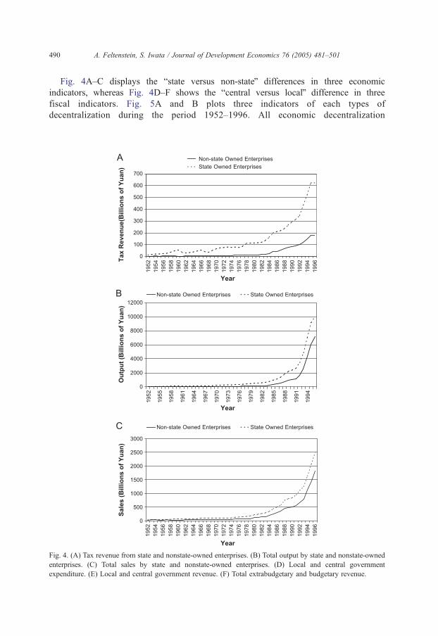
A. Feltenstein, S. Iwata / Journal of Development Economics 76 (2005) 481–501490
Fig. 4A–C displays the bstate versus non-stateQ differences in three economic
indicators, whereas Fig. 4D–F shows the bcentral versus localQ difference in three
fiscal indicators. Fig. 5A and B plots three indicators of each types of
decentralization during the period 1952–1996. All economic decentralization
Fig. 4. (A) Tax revenue from state and nonstate-owned enterprises. (B) Total output by state and nonstate-owned
enterprises. (C) Total sales by state and nonstate-owned enterprises. (D) Local and central government
expenditure. (E) Local and central government revenue. (F) Total extrabudgetary and budgetary revenue.
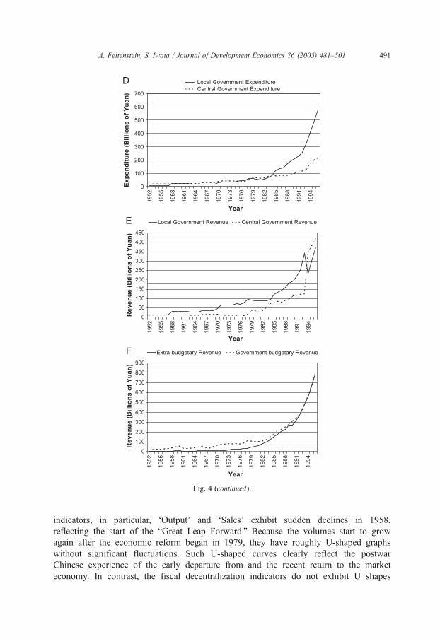
Fig. 4 (continued).
A. Feltenstein, S. Iwata / Journal of Development Economics 76 (2005) 481–501 491
indicators, in particular, dOutputT and dSalesT exhibit sudden declines in 1958,
reflecting the start of the bGreat Leap Forward.Q Because the volumes start to grow
again after the economic reform began in 1979, they have roughly U-shaped graphs
without significant fluctuations. Such U-shaped curves clearly reflect the postwar
Chinese experience of the early departure from and the recent return to the market
economy. In contrast, the fiscal decentralization indicators do not exhibit U shapes
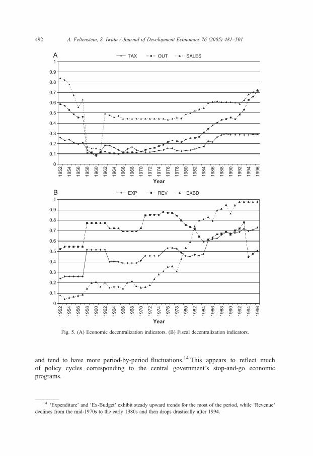
Fig. 5. (A) Economic decentralization indicators. (B) Fiscal decentralization indicators.
A. Feltenstein, S. Iwata / Journal of Development Economics 76 (2005) 481–501492
and tend to have more period-by-period fluctuations.14 This appears to reflect much
of policy cycles corresponding to the central government’s stop-and-go economic
programs.
14 dExpenditureT and dEx-BudgetT exhibit steady upward trends for the most of the period, while dRevenueTdeclines from the mid-1970s to the early 1980s and then drops drastically after 1994.
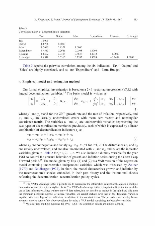
Table 3
Correlation matrix of decentralization indicators
Tax Output Sales Expenditure Revenue Ex-budget
Tax 1.0000
Output 0.8708 1.0000
Sales 0.7693 0.8321 1.0000
Expenditure 0.4553 0.2641 �0.0108 1.0000
Revenue �0.6302 �0.7408 �0.6836 0.0942 1.0000
Ex-budget 0.6518 0.5315 0.3582 0.8399 �0.2454 1.0000
A. Feltenstein, S. Iwata / Journal of Development Economics 76 (2005) 481–501 493
Table 3 reports the pairwise correlation among the six indicators. dTax,T dOutputT anddSalesT are highly correlated, and so are dExpenditureT and dExtra Budget.T
4. Empirical model and estimation method
Our formal empirical investigation is based on a 2�1 vector autoregression (VAR) with
lagged decentralization variables.15 The basic model is written as�y1t
y2t
�¼�
b10
b20
�þ�
b11
b21
�w1;t�1 þ
�b12
b22
�w2;t�1 þ
Xpj¼1
�c11j c12jc21j c22j
��y1;t�j
y2;t�j
�þ�u1t
u2t
�
ð1Þwhere y1 and y2 stand for the GNP growth rate and the rate of inflation, respectively, and
u1 and u2 are serially uncorrelated errors with mean zero vector and nonsingular
covariance matrix. The variables w1 and w2 are unobservable variables representing the
two types of decentralization mentioned previously, each of which is expressed by a linear
combination of decentralization indicators zj as
w1t ¼ a11z1t þ a12z2t þ a13z3t þ e1t
w2t ¼ a21z4t þ a22z5t þ a23z6t þ e2t ð2Þ
where aij are nonnegative and satisfy ai1+ai1+ai1=1 for i=1, 2. The disturbances e1 and e2are serially uncorrelated, and are also uncorrelated with u1 and u2, and zjt are the indicator
variables given in Table 2 for j=1, 2,. . ., 6. We also include a dummy variable for the year
1961 to control the unusual behavior of growth and inflation series during the Great Leap
Forward period.16 The model given by Eqs. (1) and (2) is a VAR version of the regression
model containing unobservable independent variables, which was discussed by Zellner
(1970) and Goldberger (1972). In short, the model characterizes growth and inflation by
the macroeconomic shocks embedded in their past history and the institutional shocks
reflecting the decentralization–recentralization policy cycles.
15 The VAR’s advantage is that it permits one to summarize the information content of the data in a multiple
time series as a set of empirical stylized facts. The VAR’s disadvantage is that it is quite inefficient in terms of the
use of data information. Since we have only 45 data points, it is not possible to include in the right hand side even
the minimum necessary number of lagged variables. We cannot include three lags of the dependent variables
together with three lags of six indicators, in addition to the constant terms. The procedure we develop below
attempts to solve some of the above problems by using a VAR model containing unobservable variables.16 We also tried multiple dummies for 1960–1962. The estimation results are almost identical.
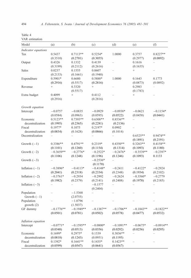
Table 4
VAR estimation
Model (a) (b) (c) (d) (e) (f)
Indicator equations
Tax 0.5437
(0.3510)
0.7113**
(0.2701)
0.5254*
(0.3055)
1.0000 0.3757
(0.2977)
0.8227**
(0.0892)
Output 0.4326
(0.3199)
0.1332
(0.2112)
0.4139
(0.2616)
– 0.1616
(0.1635)
–
Sales 0.0237
(0.2133)
0.1555
(0.1661)
0.0607
(0.1940)
– + –
Expenditure 0.5901*
(0.2916)
0.6680
(0.5517)
0.5888*
(0.2816)
1.0000 0.1643
(0.0873)
0.1773
(0.0892)
Revenue + 0.3320
(0.5517)
+ – 0.2983
(0.1783)
–
Extra budget 0.4099
(0.2916)
+ 0.4112
(0.2816)
– + –
Growth equation
Intercept �0.0757
(0.0584)
�0.0835
(0.0963)
�0.0929
(0.0595)
�0.0938*
(0.0522)
�0.0621
(0.0458)
�0.1154*
(0.0441)
Economic
decentralization
0.5123**
(0.1995)
0.7393**
(0.2365)
0.6308**
(0.2281)
0.8536**
(0.2136)
– –
Fiscal
decentralization
0.1977*
(0.0834)
0.1075
(0.1628)
0.2197*
(0.0866)
0.0902
(0.1014)
– –
Decentralization – – – – 0.6525**
(0.1891)
0.9474**
(0.2191)
Growth (�1) 0.3386**
(0.1101)
0.4791**
(0.1260)
0.2319*
(0.1154)
0.4350**
(0.1314)
0.3263**
(0.1093)
0.4158**
(0.1180)
Growth (�2) �0.3659**
(0.1106)
�0.2776*
(0.1248)
�0.2522*
(0.1196)
�0.2476*
(0.1246)
�0.3539**
(0.1093)
�0.2397*
0.1133
Growth (�3) – – �0.2536*
(0.1170)
– – –
Inflation (�1) �0.3896*
(0.2041)
�0.4113*
(0.2318)
�0.4148*
(0.2334)
�0.2411
(0.2348)
�0.4122*
(0.1934)
�0.2924
(0.2102)
Inflation (�2) �0.3761*
(0.1982)
�0.2934
(0.2379)
�0.2992
(0.2141)
�0.2624
(0.2408)
�0.3560*
(0.1978)
�0.2779
(0.2185)
Inflation (�3) – – �0.1577
(0.2404)
– – –
Population
Growth (�1)
– �1.5368
(2.0755)
– – – –
Population
growth (2)
– �1.0796
(1.5037)
– – – –
GF dummy �0.1776**
(0.0501)
�0.1949**
(0.0781)
�0.1387**
(0.0502)
�0.1706**
(0.0578)
�0.1843**
(0.0477)
�0.1822**
(0.0532)
Inflation equation
Intercept �0.0771*
(0.0348)
�0.1595**
(0.0513)
�0.0800*
(0.0356)
�0.1091**
(0.0292)
�0.0675*
(0.0256)
�0.0914**
(0.0295)
Economic
decentralization
0.1699*
(0.0818)
0.2975*
(0.1243)
0.1539
(0.0951)
0.3036**
(0.1195)
– –
Fiscal
decentralization
0.1392*
(0.0599)
0.1641**
(0.0547)
0.1435*
(0.0641)
0.1423**
(0.0567)
– –
A. Feltenstein, S. Iwata / Journal of Development Economics 76 (2005) 481–501494
Model (a) (b) (c) (d) (e) (f)
Inflation equation
Decentralization – – – – 0.3110**
(0.0983)
0.4432**
(0.1280)
Growth (�1) 0.0598
(0.0637)
0.0828
(0.0723)
0.0819
(0.0707)
0.1011
(0.0735)
0.0721
(0.0653)
0.1169
(0.0695)
Growth (�2) �0.0030
(0.0614)
�0.0043
(0.0625)
�0.0371
(0.0700)
0.0474
(0.0697)
�0.0135
(0.0627)
0.0409
(0.0641)
Growth (�3) – – 0.0566
(0.0710)
– – –
Inflation (�1) 0.4246**
(0.1152)
0.2934*
(0.1283)
0.4065**
(0.1317)
0.4647**
(0.1314)
0.4469**
(0.1157)
0.5068**
(0.1230)
Inflation (�2) �0.5386**
(0.1163)
�0.3502**
(0.1467)
�0.5260**
(0.1275)
�0.5057**
(0.1347)
�0.5350**
(0.1170)
�0.4931**
(0.1270)
Inflation (�3) – – �0.0403
(0.1393)
– – –
M1 Growth (�1) – 0.1416**
(0.033)
– – – –
M1 Growth (�2) – 0.0077
(0.0349)
– – – –
GF dummy 0.1496**
(0.0027)
0.1409**
(0.0266)
0.1441**
(0.0286)
0.1458**
(0.0323)
0.1547**
(0.0270)
0.1554 **
(0.0293)
Log likelihood 245.6336 251.5695 245.8565 240.0178 244.5202 238.0027
AIC �10.6016 �10.3128 �10.7428 �10.6675 �10.5962 �10.4287
(1) Figures in parentheses are standard errors.
(2) GF stands for Great Famine.
(3) + stands for the value of the estimate smaller than 0.0001 in magnitude.
(4) Akaike Information Criterion (AIC) is calculated according to
AIC ¼ � 2=nð Þ loglikelihoodð Þ þ 2K=nð Þwhere K is the number of parameters and n is the sample size.
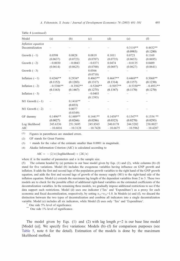
(5) The column headed by (a) pertains to our base model given by Eqs. (1) and (2), while columns (b)–(f)
stand for five variations. Model (b) includes the exogenous variables having influence on GNP growth and
inflation. It adds the first and second lags of the population growth variables to the right hand of the GNP growth
equation, and adds the first and second lags of growth of the money supply (M1) to the right-hand side of the
inflation equation. Model (c) extends the maximum lag length of the dependent variables from 2 to 3. These two
models are to check for the possible effect of additional right-hand variables on the estimated coefficients of the
decentralization variables. In the remaining three models, we gradually impose additional restrictions to see if the
data support such restrictions. Model (d) uses one indicator (dTaxT and dExpenditureT) as a proxy for each
economic and fiscal decentralization, respectively, by setting a11=a21=1.0. In Models (e) and (f), we discard the
distinction between the two types of decentralization and combine all indicators into a single decentralization
variable. Model (e) includes all six indicators, while Model (f) uses only dTaxT and dExpenditureT.* One side 5% level of significance.** One side 1% level of significance.
Table 4 (continued)
A. Feltenstein, S. Iwata / Journal of Development Economics 76 (2005) 481–501 495
The model given by Eqs. (1) and (2) with lag length p=2 is our base line model
[Model (a)]. We specify five variations: Models (b)–(f) for comparison purposes (see
Table 5, note 6 for the detail). Estimation of the models is done by the maximum
likelihood method.
A. Feltenstein, S. Iwata / Journal of Development Economics 76 (2005) 481–501496
5. Empirical results
Our interest centers on the following two questions: First, how important are the two
types of decentralization variables in describing economic growth and inflation in the
postwar economy in China? Second, is there any drastic regime shift in the structure of the
economy in China between pre- and post-reform periods?
5.1. Impact of decentralization
The estimation results for the VAR models are reported in Table 4. The values of the
Akaike Information Criterion (AIC) are similar for all models. There is no single model
that is especially unfavorable from this criterion. The important findings are summarized
as follows: First, two types of decentralization variables, economic and fiscal, are found to
be positive and highly significant (at the 1% or 5% level in most cases) in both the GNP
growth and inflation equations of Models (a)–(d). The single decentralization variables in
Models (e) and (f) are even more significant in both equations. Second, in Models (a)–(d)
the economic decentralization variable is relatively more significant in the GNP growth
equation, while the fiscal decentralization variable is relatively more significant in the
inflation equation.17
The strong association between economic decentralization and GNP growth supports
the view that the institutional change toward a more competitive market has been a cause
of growth in China. The similarly strong association between fiscal decentralization and
inflation favors the view that fiscal federalism often leads to inflation.
In order to go a step further in capturing the structural dynamics of the relation, we
estimate a structural VAR model by adding the decentralization variable to system (1) and
imposing identification restrictions.18 The coefficient estimates for the first two equations
are very close (not shown here) to those of Model (f) in Table 5. Fig. 6 presents the
17 Other findings are (i) highly significant lagged variables in the growth equation and in the inflation
equation are the dependent variables own first and second lags. No lagged growth variables are significant in the
inflation equation. The F-test result (not shown) implies that growth does not Granger cause inflation. (ii) The
estimated weights for the unobserved decentralization variables reveal that dTaxT and dExpenditureT dominate
other variables in economic and fiscal decentralization, respectively. dSalesT has almost no contribution to
explaining GNP growth and inflation. (iii) The strong significance of Great Leap Forward dummies in both
growth and inflation equations shows 1961 to be an outlier.18 For simplicity we do not distinguish fiscal and economic decentralization. The decentralization variable is
constructed using the weights estimated in Model (f). The model is given by
yt ¼ b0 þXpj¼1
&jyt�j þ ut
where yt=[ y1t,y2t,wt], b0 is a 3�1 vector , and &j is a 3�3 matrix of constants. To identify the decentralization
shock, we assume that decentralization is contemporaneously affected by neither the growth nor inflation shocks.
In other words, we assume
C ¼c11 0 0
c21 c22 c23c31 c32 c33
35
24
where ut=Ce t and Var(et)=I3, an identity matrix. We include up to third lags for all three variables in our VAR
model.
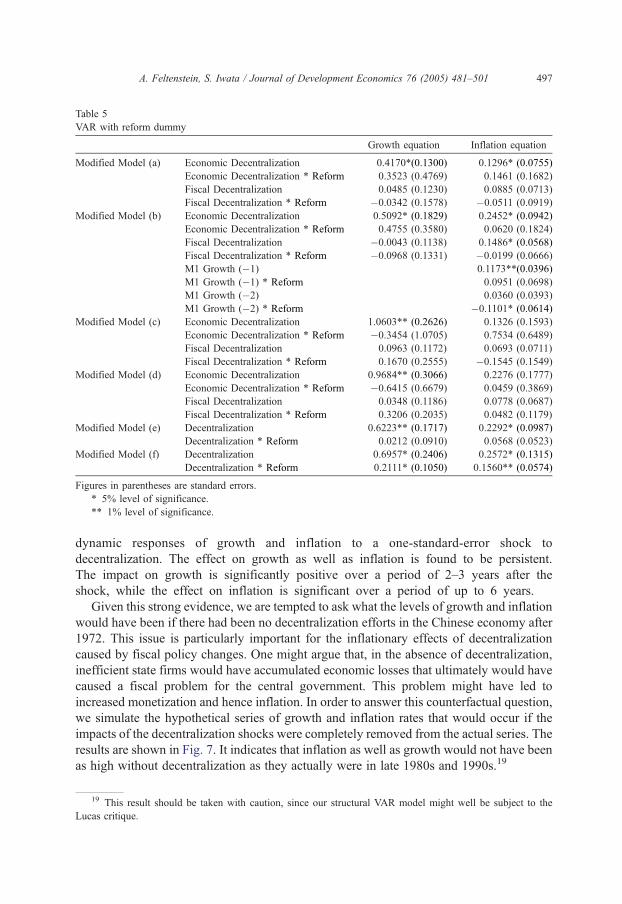
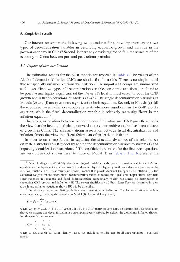
Table 5
VAR with reform dummy
Growth equation Inflation equation
Modified Model (a) Economic Decentralization 0.4170*(0.1300) 0.1296* (0.0755)
Economic Decentralization * Reform 0.3523 (0.4769) 0.1461 (0.1682)
Fiscal Decentralization 0.0485 (0.1230) 0.0885 (0.0713)
Fiscal Decentralization * Reform �0.0342 (0.1578) �0.0511 (0.0919)
Modified Model (b) Economic Decentralization 0.5092* (0.1829) 0.2452* (0.0942)
Economic Decentralization * Reform 0.4755 (0.3580) 0.0620 (0.1824)
Fiscal Decentralization �0.0043 (0.1138) 0.1486* (0.0568)
Fiscal Decentralization * Reform �0.0968 (0.1331) �0.0199 (0.0666)
M1 Growth (�1) 0.1173**(0.0396)
M1 Growth (�1) * Reform 0.0951 (0.0698)
M1 Growth (�2) 0.0360 (0.0393)
M1 Growth (�2) * Reform �0.1101* (0.0614)
Modified Model (c) Economic Decentralization 1.0603** (0.2626) 0.1326 (0.1593)
Economic Decentralization * Reform �0.3454 (1.0705) 0.7534 (0.6489)
Fiscal Decentralization 0.0963 (0.1172) 0.0693 (0.0711)
Fiscal Decentralization * Reform 0.1670 (0.2555) �0.1545 (0.1549)
Modified Model (d) Economic Decentralization 0.9684** (0.3066) 0.2276 (0.1777)
Economic Decentralization * Reform �0.6415 (0.6679) 0.0459 (0.3869)
Fiscal Decentralization 0.0348 (0.1186) 0.0778 (0.0687)
Fiscal Decentralization * Reform 0.3206 (0.2035) 0.0482 (0.1179)
Modified Model (e) Decentralization 0.6223** (0.1717) 0.2292* (0.0987)
Decentralization * Reform 0.0212 (0.0910) 0.0568 (0.0523)
Modified Model (f) Decentralization 0.6957* (0.2406) 0.2572* (0.1315)
Decentralization * Reform 0.2111* (0.1050) 0.1560** (0.0574)
Figures in parentheses are standard errors.
* 5% level of significance.
** 1% level of significance.
A. Feltenstein, S. Iwata / Journal of Development Economics 76 (2005) 481–501 497
dynamic responses of growth and inflation to a one-standard-error shock to
decentralization. The effect on growth as well as inflation is found to be persistent.
The impact on growth is significantly positive over a period of 2–3 years after the
shock, while the effect on inflation is significant over a period of up to 6 years.
Given this strong evidence, we are tempted to ask what the levels of growth and inflation
would have been if there had been no decentralization efforts in the Chinese economy after
1972. This issue is particularly important for the inflationary effects of decentralization
caused by fiscal policy changes. One might argue that, in the absence of decentralization,
inefficient state firms would have accumulated economic losses that ultimately would have
caused a fiscal problem for the central government. This problem might have led to
increased monetization and hence inflation. In order to answer this counterfactual question,
we simulate the hypothetical series of growth and inflation rates that would occur if the
impacts of the decentralization shocks were completely removed from the actual series. The
results are shown in Fig. 7. It indicates that inflation as well as growth would not have been
as high without decentralization as they actually were in late 1980s and 1990s.19
19 This result should be taken with caution, since our structural VAR model might well be subject to the
Lucas critique.
Fig. 6. Impulse responses to the decentralization shock.
A. Feltenstein, S. Iwata / Journal of Development Economics 76 (2005) 481–501498
5.2. Is the post-reform period a new paradigm?
Our models implicitly assume that the Chinese economy has been reacting to
decentralization in the same manner before and after the reform. To determine whether this
assumption is consistent with the data, we first conduct tests for a structural break in 1979.
The standard Chow test based on Model (d) (with F-ratios 1.9246 and 1.7507 for the
growth and inflation equation, respectively) cannot reject the null hypothesis of no
structural break. Similar results are obtained for the other models using likelihood ratio
tests. These results are particularly interesting when compared with the results obtained
when the VAR does not include any decentralization variables. The Chow test statistics
without decentralization variables (3.56 and 4.68 for the growth and inflation equation) are
larger than the critical value at the 5% level (2.53). Failure to include decentralization
indicators would therefore lead to erroneous conclusions supporting a structural break in
1979.20
Given little evidence of structural change in the entire process, we next investigate the
possibility of a change in the impact of decentralization on the economy after 1979. To test
this assumption we modify our Models (a)–(c) by replacing bij with bij+dijdt�1 for i=1, 2
and j=1, 2 in Eq. (1), where dt is a reform dummy defined by dt=1 for tz1979 and=0
otherwise.21 In all modified models except for Model (f) in Table 5, we find no interaction
terms with the reform dummy to be significant.22
20 Perhaps the less than expected support for a structural break might be a result of singling out 1979 as a
break point. The results of the CUSUM test (Brown et al., 1975) (not shown), however, provide clear evidence
against this view. No structural change is observed during the period from 1975 to 1996.21 We call the resulting models the dmodified Models (a)–(c)T. If dij is significantly positive in this model
while is bij not, then the effect of decentralization observed in Table 4 may be specific to the reform period. If bij
is significantly positive while d ij is not, then there is no change in the reaction of the economy to the
decentralization shocks before and after the reform started.22 Although the modified Model (f) shows a somewhat significant effect of the reform dummy, especially in
the inflation equation, we cannot reject the null hypothesis of no change in the impact of the decentralization after
1979. The stability of the coefficients of the decentralization variables in the growth and inflation equations is
confirmed by the results of the rolling vector autoregressions (not shown). Except for the initial period of the
inflation equation, the parameters appear to be stable.
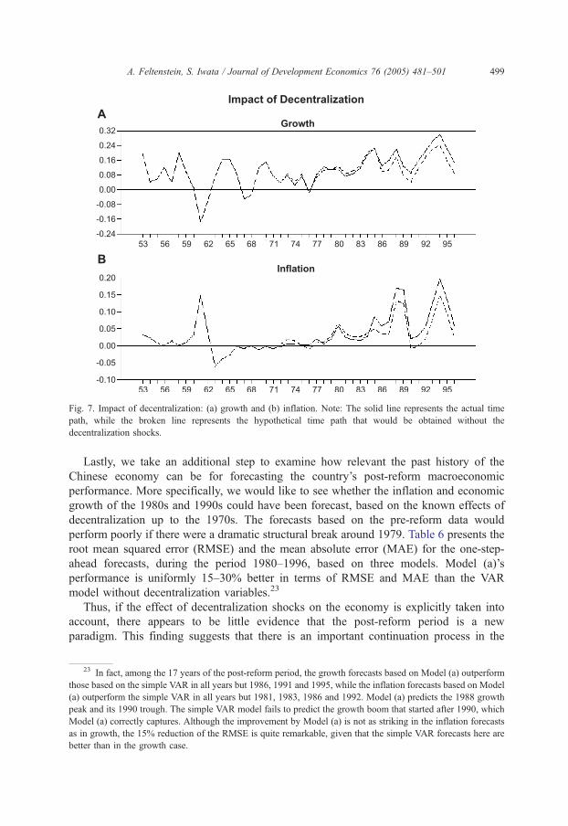
Fig. 7. Impact of decentralization: (a) growth and (b) inflation. Note: The solid line represents the actual time
path, while the broken line represents the hypothetical time path that would be obtained without the
decentralization shocks.
A. Feltenstein, S. Iwata / Journal of Development Economics 76 (2005) 481–501 499
Lastly, we take an additional step to examine how relevant the past history of the
Chinese economy can be for forecasting the country’s post-reform macroeconomic
performance. More specifically, we would like to see whether the inflation and economic
growth of the 1980s and 1990s could have been forecast, based on the known effects of
decentralization up to the 1970s. The forecasts based on the pre-reform data would
perform poorly if there were a dramatic structural break around 1979. Table 6 presents the
root mean squared error (RMSE) and the mean absolute error (MAE) for the one-step-
ahead forecasts, during the period 1980–1996, based on three models. Model (a)’s
performance is uniformly 15–30% better in terms of RMSE and MAE than the VAR
model without decentralization variables.23
Thus, if the effect of decentralization shocks on the economy is explicitly taken into
account, there appears to be little evidence that the post-reform period is a new
paradigm. This finding suggests that there is an important continuation process in the
23 In fact, among the 17 years of the post-reform period, the growth forecasts based on Model (a) outperform
those based on the simple VAR in all years but 1986, 1991 and 1995, while the inflation forecasts based on Model
(a) outperform the simple VAR in all years but 1981, 1983, 1986 and 1992. Model (a) predicts the 1988 growth
peak and its 1990 trough. The simple VAR model fails to predict the growth boom that started after 1990, which
Model (a) correctly captures. Although the improvement by Model (a) is not as striking in the inflation forecasts
as in growth, the 15% reduction of the RMSE is quite remarkable, given that the simple VAR forecasts here are
better than in the growth case.
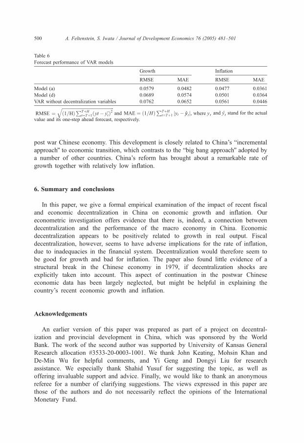
Table 6
Forecast performance of VAR models
Growth Inflation
RMSE MAE RMSE MAE
Model (a) 0.0579 0.0482 0.0477 0.0361
Model (d) 0.0689 0.0574 0.0501 0.0364
VAR without decentralization variables 0.0762 0.0652 0.0561 0.0446
RMSE ¼ffiffiffiffiffiffiffiffiffiffiffiffiffiffiffiffiffiffiffiffiffiffiffiffiffiffiffiffiffiffiffiffiffiffiffiffiffiffiffiffiffiffiffiffiffiffiffiffi1=Hð Þ
PTþHt¼Tþ1 yt � ytð Þ2
qand MAE ¼ 1=Hð Þ
PTþHt¼Tþ1 jyt � yyt j, where yt and yt stand for the actual
value and its one-step ahead forecast, respectively.
A. Feltenstein, S. Iwata / Journal of Development Economics 76 (2005) 481–501500
post war Chinese economy. This development is closely related to China’s bincremental
approachQ to economic transition, which contrasts to the bbig bang approachQ adopted by
a number of other countries. China’s reform has brought about a remarkable rate of
growth together with relatively low inflation.
6. Summary and conclusions
In this paper, we give a formal empirical examination of the impact of recent fiscal
and economic decentralization in China on economic growth and inflation. Our
econometric investigation offers evidence that there is, indeed, a connection between
decentralization and the performance of the macro economy in China. Economic
decentralization appears to be positively related to growth in real output. Fiscal
decentralization, however, seems to have adverse implications for the rate of inflation,
due to inadequacies in the financial system. Decentralization would therefore seem to
be good for growth and bad for inflation. The paper also found little evidence of a
structural break in the Chinese economy in 1979, if decentralization shocks are
explicitly taken into account. This aspect of continuation in the postwar Chinese
economic data has been largely neglected, but might be helpful in explaining the
country’s recent economic growth and inflation.
Acknowledgements
An earlier version of this paper was prepared as part of a project on decentral-
ization and provincial development in China, which was sponsored by the World
Bank. The work of the second author was supported by University of Kansas General
Research allocation #3533-20-0003-1001. We thank John Keating, Mohsin Khan and
De-Min Wu for helpful comments, and Yi Geng and Dongyi Liu for research
assistance. We especially thank Shahid Yusuf for suggesting the topic, as well as
offering invaluable support and advice. Finally, we would like to thank an anonymous
referee for a number of clarifying suggestions. The views expressed in this paper are
those of the authors and do not necessarily reflect the opinions of the International
Monetary Fund.
A. Feltenstein, S. Iwata / Journal of Development Economics 76 (2005) 481–501 501
References
Bell, M., Khor, H.E., Kochhar, K., 1993. China at the Threshold of a Market Economy. International Monetary
Fund, Washington, DC.
Brandt, L., Zhu, X., 2000. Redistribution in a decentralized economy: growth and inflation in China under reform.
Journal of Political Economy 108, 422–439.
Broadman, H.G., 1995. Meeting the challenge of Chinese Enterprise Reform. World Bank Discussion Papers 283.
Brown, R.L., Durbin, J., Evans, J.M., 1975. Techniques for testing the constancy of regression relationships over
time. Journal of the Royal Statistical Society. Series B 37, 149–163.
Dollar, D., 1990. Economic reform and allocative efficiency in China’s state-owned industry. Economic
Development and Cultural Change 34, 89–105.
Easterly, W., Rebelo, S., 1993. Fiscal policy and economic growth: an empirical investigation. Journal of
Monetary Economics 32, 417–458.
Feltenstein, A., Ha, J., 1991. Measurement of repressed inflation in China: the lack of coordination between
monetary policy and price controls. Journal of Development Economics 36, 279–294.
Feltenstein, A., Lebow, D., Van Wijnbergen, S., 1990. Savings, commodity market rationing and the real rate of
interest in China. Journal of Money, Credit and Banking, 234–252 (May).
Goldberger, A., 1972. Maximum-likelihood estimation of regressions containing unobservable independent
variables. International Economic Review 13.
Groves, T., Hong, Y., McMillan, J., Naughton, B., 1994. Autonomy and incentives in Chinese state enterprises.
Quarterly Journal of Economics Review, 183–209.
Hofman, B., 1993. An analysis of Chinese fiscal data over the reform period. China Economic Review 4, 213–230.
Jefferson, G.H., Sigh, I., Xing, J., Zhang, Z., 1999. China’s industrial performance: a review of recent findings.
In: Jefferson, G.H., Singh, I. (Eds.), Enterprise Reform in China: Ownership, Transition, and Performance.
Oxford University Press, New York.
Jin, H., Qian, Y., Weingast, B.R., 1999. Regional decentralization and fiscal incentives: federalism, Chinese style,
Working paper, Department of Economics, University of Maryland.
Lardy, Nicholas R., 1998. China’s Unfinished Economic Revolution. Brooking Institution Press, Washington, DC.
Ma, G., 1995. Income Distribution in the 1980s. China’s Quiet Revolution. St. Martin Press, New York.
Ma, J., 1997. Intergovernmental Relations and Economic Management in China. MacMillan, London.
Maskin, E.S., 1999. Recent theoretical work on the soft budget constraint. American Economic Review 89,
421–425.
Naughton, Barry, 1995. Growing Out of the Plan: Chinese Economic Reform, 1978–1993. Cambridge University
Press, New York.
Prudhomme, R., 1994. bThe dangers of decentralization.Q World Bank, unpublished manuscript.
Qian, Yingyi, Xu, Chenggang, 1998. Innovation and bureaucracy under soft and hard budget constraints. Review
of Economic Studies 66, 156–164.
Tseng, W., Khor, H.E., Kochar, K., Mihaljek, D., Burton, D., 1994. Economic Reform in China: A New Phase.
International Monetary Fund, Washington, DC.
Tanzi, V., 1995. Fiscal Federalism and Decentralization: A Review of Some Efficiency and Macroeconomics
Aspects, ABCDE Conference. The World Bank, Washington DC.
World Bank, 1994. China: Country Economic Memorandum, Macroeconomic Stability in a Decentralized
Economy. The World Bank, Washington DC.
World Bank, 1996. The Chinese Economy: Fighting Inflation, Deepening Reforms. The World Bank,
Washington, DC.
World Bank, 1997. China 2020: Development Challenges in the New Century. The World Bank, Washington, DC.
Yusuf, S., 1994. China’s macroeconomic performance and management during transition. Journal of Economic
Perspectives 8, 71–92.
Zellner, A., 1970. Estimation of regression relationships containing unobservable independent variables.
International Economic Review, 11.