Deadbands, Droop and Inertia Impact on PowerSystem Frequency Distribution

Petr Vorobev, Member, IEEE, David M. Greenwood, Member, IEEE, John H. Bell,

Janusz W. Bialek, Fellow, IEEE, Philip C. Taylor, Senior Member, IEEE, and Konstantin Turitsyn, Member, IEEE

Abstract—Power system inertia is falling as more energy issupplied by renewable generators, and there are concerns aboutthe frequency controls required to guarantee satisfactory systemperformance. The majority of research into the negative effectof low inertia has focused on poor dynamic response followingmajor disturbances, when the transient frequency dip can becomeunacceptable. However, another important practical concern –keeping average frequency deviations within acceptable limits– was mainly out of the sight of the research community. Inthis manuscript we present a method for finding the frequencyprobability density function (PDF) for a given power system. Wepass from an initial stochastic dynamic model to deterministicequations for the frequency PDF, which are analyzed to uncoverkey system parameters influencing frequency deviations. Weshow that system inertia has little effect on the frequencyPDF, making virtual inertia services insufficient for keepingfrequency close to nominal under ambient load fluctuations. Weestablish, that aggregate system droop and deadband width arethe only parameters that have major influence on the averagefrequency deviations, suggesting that energy storage might be anexcellent solution for tight frequency regulation. We also showthat changing the governor deadband width does not significantlyaffect generator movement..

Index Terms—Frequency control, droop control, deadbands,low inertia grids, frequency fluctuations.

I. INTRODUCTION

In electric power systems, primary and secondary frequency

controls are aimed at maintaining a stable system frequency

and restoring power balance [1]. During any major disturbance

(typically a loss of a generating unit) frequency deviates

rapidly from the nominal, triggering all generators partici-

pating in primary response to quickly readjust their output

and restore the power balance. However, even during pre-

fault operation, frequency can drift from its nominal value due

to stochastic load fluctuations, and generators participating in

frequency control constantly readjust their power output in

response. The ability of the system to keep frequency within

This work was supported in part by Skoltech-MIT Next Generationprogram, in part by MIT Undergraduate Research Opportunities Program(UROP), and in part by the Engineering and Physical Sciences ResearchCouncil (EPSRC) under grant number EP/K002252/1

P.Vorobev and J. W. Bialek are with the Skolkovo Institute of Scienceand Technology (Skoltech), Moscow, Russia E-mail: p.vorobev@skoltech.ru,J.Bialek@skoltech.ru

J.H.Bell is with Department of Mechanical Engineering, MassachusettsInstitute of Technology. E-mail: jhbell@mit.edu

D.M. Greenwood and P.C.Taylor are with the School of Electrical andElectronic Engineering, Newcastle University, Newcastle Upon Tyne, U.K.Email: : david.greenwood@ncl.ac.uk; phil.taylor@ncl.ac.uk

K.Turitsyn was with Department of Mechanical Engineering,MassachusettsInstitute of Technology. E-mail: turitsyn@gmail.com

certain limits the majority of the time is one of the major

performance characteristics of a power system.

A number of metrics exist to assess frequency regulation

adequacy; one of the most cited sets of metrics is related to

transient frequency response following a contingency [2]. The

main performance indices considered are the rate of change

of frequency (ROCOF), the frequency nadir – the maximum

frequency drop following a contingency – and a quasi-steady

state frequency deviation [3], [4]. The three major system pa-

rameters which affect these indices are: overall system inertia,

effective droop coefficient, and governor/turbine delays. The

system inertia is by far the most discussed parameter in re-

search literature due to the fact that, unlike the droop response,

it can not be manually tuned; instead, it is determined by the

amount of rotating mass that is synchronously coupled to the

system.

Overall system inertia is considered to be one of the major

factors affecting both ROCOF and frequency nadir during a

transient [3], [5], [6], and decreasing system inertia is one

of the main parameters limiting further increases in renew-

able penetration [7], [8]. Numerous papers are dedicated to

renewable energy resources participating in frequency control,

mostly focusing on wind turbines interfaced with doubly fed

induction machines [9]–[11]. Such a synthetic inertial and

droop response, however, requires continuous operation of the

renewable generator below the maximum power point, which

constitutes a non-zero cost of such services.

Transient frequency response following major disturbances

is not the only metrics that should be considered when assess-

ing frequency regulation adequacy. The system should also be

able to keep the average frequency deviation over extended

periods of time within certain limits. Thus, the so-called

Control Performance Standards (CPS1 and CPS2) [12] issued

by NERC in late 90s imposed a limit on a root mean square

(RMS) frequency deviation over a one year period; a detailed

description, with particular target values, can be found in [13].

While the influence of frequency control settings and power

systems parameters on the transient frequency response has

been extensively studied, there is still little research available

on how those settings affect the RMS frequency deviation. One

of the reasons is that dynamic equations with stochastic terms

should be considered in order to analyze the average frequency

deviations. Moreover, unlike for transient frequency response,

where a single dynamic simulation can provide enough data,

multiple simulations or a single simulation over an extended

period of time are required to get statistically valid results.

A comprehensive framework for modelling power sys-

tem dynamics with stochastic perturbations represented by

an Ornstein-Uhlenbeck process was developed in [14]. The

method was then applied to perform a number of simulations

for transient stability assessment. In a later publication [15]

the authors offered a method for obtaining the noise param-

eters of the load using micro-PMU (Phasor Measurement

Unit) measurement data. In [16] a direct simulation based

on stochastic model was performed to study the frequency

probability distribution function and the results were compared

to real-life data for Irish power system. In a recent study [17]

power system response to random ambient fluctuations, which

can be obtained from PMU data, was used to estimate the

dynamic frequency response at different buses following a

localized disturbance. Finally, the series of works [18]–[20]

presented a study of the compliance of Texas power system

(ERCOT) automatic generation control settings to NERC CPS

standards.

Instead of running lengthy numerical simulations, one can

derive an explicit equation for the probability density function

(PDF) of system frequency. Under the assumption, that the

underlying load fluctuations can be modelled as white noise,

the derivation is straightforward and leads to the, so-called,

Fokker-Planck equation. Such an approach was used in [21]

for probabilistic assessment of power system transient stability.

While the use of Fokker-Planck equation requires certain as-

sumptions about the noise type, it allows one to explicitly find

the probability distribution functions for different system states

bypassing the need for lengthy direct numerical simulations.

Thus, in [22] the performance of different primary frequency

control methods in the presence of random load fluctuations

and measurement noise was analyzed by calculating RMS fre-

quency deviation. Moreover, for linear system representation,

a semi-analytic solution is available which allows for explicit

analysis of the influence of different system parameters on

the probability distribution functions of it’s states. In an early

paper [23] statistical analysis was performed to compare CPS1

and CPS2 standards assuming Gaussian form for probability

distribution function of frequency.

In this manuscript we apply the Fokker-Planck equation to

study probability density functions of frequency deviations in

power systems. We explicitly study the influence of inertia,

droop coefficients, secondary frequency control settings, tur-

bine time-constant and governor deadbands on the distribution

function of frequency deviations. Based on our analysis we

make predictions on how the frequency deviations will change

in future systems with more renewable generation, and suggest

possible ways of improving the performance of frequency

control.

The main contributions of the present manuscript are as

follows:

1) A Fokker-Planck equation for the frequency PDF is

derived and explicitly solved. The influence of system

parameters on the frequency PDF is explicitly estab-

lished and analyzed.

2) Inertia is shown to have little effect on the RMS

frequency deviation, contrary to it’s role in transient

frequency response to contingencies.

3) We demonstrate the effect of governor deadbands, show-

ing that simultaneous decrease in deadbands across the

whole system reduced the RMS frequency deviation

without leading to significantly higher generator wear-

and-tear.

II. MODELLING APPROACH

In this section and Section III we describe our general

approach to studying the long-term frequency distribution in

power systems. Our main purpose is to establish a model that

enables the study of how different system parameters and

control settings affect the long-term frequency distribution.

We start from the general dynamic model with stochastic

perturbations, which is then used to derive an equation for

the frequency deviations probability density function (PDF).

We initially consider a power system with the vector of its

states denoted as x(t) (with N dimensions), for which we

write the set of dynamic equations in a general form:

x(t) = µ(x, t) +Bξ(t) (1)

here µ(x, t) represents the deterministic part of the power

system dynamics, and is usually referred to as the drift term

(in general it is a non-linear function of state vector x with

explicit dependence on time). Stochastic perturbations are

characterized by the diffusion term Bξ(t) where B is an

N×M matrix and ξ(t) is the M -dimensional vector of white

noise (which can be defined as the time derivative of the M -

dimensional Wiener process) with the following properties:

E[ξi(t)] = 0; E[ξi(t1)ξk(t2)] = δikδ(t1 − t2) (2)

where δik is the Kronecker delta and δ(t) is the Dirac delta-

function.One can directly simulate the dynamics caused by the

system (1) (this system in an even more general form was also

reported in [14] and [16]) with some generated white noise

signal and then infer the distribution function for the system

states from the results of these simulations. However, large,

computationally intensive simulations would be needed to

obtain a sufficiently smooth distribution functions. Moreover,

such a direct numerical method will provide limited insight

into the system. As an illustration, Fig.1 provides a histogram

for frequency deviations in the Great Britain (GB) power

system for two separate days - the source is 1 s resolution fre-

quency measurements data available from National Grid [24].

It is evident that on a one-day horizon frequency deviations do

not provide statistically reliable picture – the two histograms in

Fig.1 are very different. On the other hand, averaging over one-

month period is sufficient, which is illustrated by the Fig. 2

where the histograms of frequency deviations for two different

months look almost identical.A natural way of dealing with the shortcomings of direct nu-

merical simulations is to consider probability density function

(PDF) F(x, t) for system states. Under the assumption that

the noise in (1) is white, it is possible to write a deterministic

equation for the PDF. Following standard rules one can derive

the Fokker-Planck equation for F(x, t) [25]:

∂

∂tF(x, t) = −∇T [µF(x, t)] +∇TD∇F(x, t) (3)

-200 -100 -50 0 50 100 2000

250

500

750

1000

1250

Δω (mHz)

NumberofSamples

Fig. 1. Histograms of measured frequency deviations in GB power grid fortwo different days: day 1 - green, day 2 - red.

-200 -100 -50 0 50 100 2000

10000

20000

30000

Δω (mHz)

NumberofSamples

Fig. 2. Histograms of measured frequency deviations in GB power grid fortwo consecutive months, marked by green and red. As can be seen, twohistograms almost coincide.

where ∇ is the Nabla-operator over the space of system states

and D is the diffusion matrix defined as D = BBT /2.

Solution of equation (3) provides a PDF of all system states

x as a function of time. For finding probability density of a

certain state over a long period of time, a stationery form of

equation (3) with zero left-hand side can be used:

∇TD∇F(x, t)−∇T [µF(x, t)] = 0 (4)

In the present manuscript we are interested in the statistical

behaviour of frequency deviations on the timescales of months

(eg. Fig.2), therefore equation (4) will be used throughout the

manuscript.

Both equations (3) and (4) are in general non-linear and

solving them for a large system can be very difficult. However,

both these equation can be efficiently solved for a system

of arbitrary size in a very important case when the drift

term µ(x, t) can be represented as linear function of system

states x with some constant state matrix A. In this case the

corresponding dynamic equations (1) reduce to:

x(t) = Ax+Bξ(t) (5)

If the dynamic system (5) is stable (which we assume, as we

are investigating the pre-fault frequency distributions) then the

stationery equation (4) has solution of the form [25]:

F(x) = (det|2πC|)−1/2 · exp(

−1

2xTC−1x

)

(6)

where the co-variance matrix C is symmetric positive definite

and satisfies the following equation:

AC+CAT = −D (7)

This matrix equation can be solved numerically for a system

of arbitrary dimensions. For the systems with smaller number

of states an analytic solution is possible.

It is true that, in general, the dynamics of a power system is

non-linear. However, linear approximation can be effectively

used if the magnitudes of perturbations are small. As is seen

from the Fig.2, most of the time frequency fluctuations are

within ±100mHz, which is around 0.2% of the nominal value.

Since in this study we are interested in frequency statistical

properties, rather than separate large-deviation events, it is

justified to start form a linearized dynamic model, since it

provides an insight into the problem. Therefore, in Section

III we will assume linear frequency dynamics, validation of

our findings on fully non-linear models will be performed in

Section IV.

III. SOLUTION OF FOKKER-PLANCK EQUATION

In this section we provide a detailed analysis of the solution

of the Fokker-Planck equation for different system models - we

explicitly consider the effects of inertia, turbine time-constant,

secondary control and deadbands. We establish the main

parameters affecting the frequency deviations and provide

references to possible practical outcomes of our findings.

To study frequency fluctuations, we will consider only the

dynamics of the center of inertia (COI) of a power system,

which is justified by the fact that frequency dynamics time-

scales (starting at several seconds) are much larger than the

timescales of inter-area modes as well as dynamic phenomena

associated with high-order generator models [26]. The ade-

quacy of this single area (or single bus) model for frequency

dynamics representation was confirmed by numerous studies

(for eg. [6], [27], [28]). In Section IV we will perform the

validation on a bigger system.

A. Basic Model

We start from a simple model, in which a power system

with only primary frequency control is considered: governor

deadbands, turbine time-constants and secondary frequency

control are assumed to be absent in this initial model. We

assumed that the load stochastic dynamics can be represented

as an Ornstein-Uhlenbeck Process (OUP) [14], [16], [29], [30].

Under these assumptions the system dynamic equations are:

2Hu = −αu− p (8a)

p = − 1

τpp+ bξ (8b)

where we used the following denotations: H - is the system

aggregate inertia time constant, u - per unit frequency devia-

tion from the nominal (i.e. u(t) = (ω(t)−ω0)/ω0), α = 1/R -

is the inverse aggregate dimensionless droop coefficient of the

system (including both generator response and load sensitivity

to frequency), p - per unit load deviation from the base value,

τp is the load fluctuations mean reversal time and b is the

noise amplitude. Instead of b it is more convenient to use the,

so-called, diffusion coefficient D = b2/2. [29].

The stationary Fokker-Planck equation for the combined

frequency and power probability density function F(u, p)

corresponding to the stochastic system (8) can be derived using

(4):

D∂2F∂p2

+1

τp

∂(p · F)

∂p+

1

2H

∂

∂u

[

(αu+ p)F]

= 0 (9)

This equation can be explicitly solved to provide a normal

distribution for F(u, p):

F(u, p) =1

2πκχexp

[

− (p+ αu)2

2κ2− u2

2χ2

]

(10)

with variances κ2 and χ2 given by:

κ2 =2τpDH

2H + ατp; χ2 =

τ2pD

α(2H + ατp)(11)

Function F(u, p) in (10) gives the simultaneous probability

density for frequency and load deviations u and p. The

probability density function for frequency only - F (u) - can

be found from F(u, p) by means of integration over p:

F (u) =

∫ +∞

−∞

F(u, p)dp (12)

Performing integration of (10) over all values of p we find:

F (u) =1√2πσ2

e−u2

2σ2 (13)

with the following closed-form expression for frequency stan-

dard deviation:

σ =

(

Dτ2pα(2H + ατp)

)1/2

(14)

The value of this solution is that it allows one to calculate

the RMS frequency deviation, provided parameters of the

power system are known. In practice, the aggregate inertia

H and inverse droop α are readily available; conversely,

both load mean reversal time τp and diffusion coefficient Dare difficult to measure directly. However, one can use the

formula (14) to predict the effect of the change in inertia

and/or aggregate droop on the frequency deviations provided

the loading conditions do not change significantly.The denominator of expression (14) can be further sim-

plified by considering realistic estimations for the system

parameters: inertia term H is around 5−6 s or smaller for real-

life systems [6], [31], while α – the inverse droop – is typically

in the interval of ∼ 10−20 depending on the number of units

directly participating in primary response [32]. Therefore, the

inertial term in the denominator of (14) is small if the load

mean reversal time τp is significantly greater than ∼ 1 s.

Different estimations for τp are cited in literature [14]–[16],

most of them being well above 1 s. An approximate estimation

for the lower bound on τp can be inferred from considering an

average duration of either low or high frequency events from

historical data. Thus, an average duration of about ∼ 30 s was

cited for US Eastern Interconnection in [33], and a similar

value was obtained in [34] from analysis of the GB system

data. Therefore, in the following we will assume that condition

ατp ≫ H is satisfied. Under this assumption the expression

(14) can be further simplified:

σ =

√

Dτp

α(15)

In this form, the RMS frequency deviation appears to be

independent of the system inertia. Another way of stating this

fact is to calculate the sensitivity of the frequency standard

deviation to changes in the inertia value, given by the formula:

νH =dσ

dH(16)

Differentiating equation (14) we find that νH = −0.19mHz/s(for the values of power system parameters from Table I).This

means that the change of the system inertia constant by

1 s leads to the change of RMS frequency deviation only

by 0.19 mHz in the opposite direction. To avoid confusion,

we once again emphasize that we are only considering the

frequency fluctuations under the ambient load perturbations.

In the case of a sudden major disturbance (such as a loss

of a generating unit), inertia is one of the most important

parameters determining the depth of the frequency dip, and

has already been shown to be one of the main limiting factors

for renewables penetration [2], [4].

Determining the real-life values of system-wide diffusion

D and load reversal time τp would require observation of the

total load fluctuations over the extended period of time, and

subsequent statistical analysis. According to (15) the values

of both parameters can not be obtained from the data on the

system frequency only. However, the product D · τp can be

inferred from the measurements of frequency distribution. In

the rest of the paper we will assume the value of load mean

reversal time τp = 30 s as a base value (unless otherwise

is specified). For the load diffusion coefficient we will use

D = 6 ·10−6 s−1 which provides the value of RMS frequency

deviation close to that obtained from the real-life GB system

data [24]. We will also assume that the aggregate value of

inverse droop provided by generators to be αg = 11 (this

value for GB system is taken from [35]) and assume the load

sensitivity to frequency to be 1.5 p.u., which yields a total

inverse system droop of α = αg + αL = 12.5. The base

values of the parameters used are summarized in Table I.

B. Secondary Frequency Control

Let us now investigate the role of secondary control on the

frequency fluctuations. We assume that secondary control is

realized through an integral term, which should be added to

the right-hand side of equation (8a). Instead of (8), the system

of dynamic equations becomes:

2Hu =− αu− p−Kiθ (17a)

θ = u (17b)

p =− 1

τpp+ bξ (17c)

where Ki is the secondary control parameter with a typical

value around ∼ 0.05 s−1 [36]. The corresponding probability

density function F(u, p, θ) is now a function of three variables

and has a Gaussian form of (6). Using (5), (17), and (7) one

can find the corresponding covariance matrix. After integration

over p and θ, similar to (12), the corresponding frequency

probability density function F (u) can be obtained. It has

the same form as (14) with the following value of standard

deviation σ:

σ =

(

Dτ2pα(2H + ατp +Kiτ2p )

)1/2

(18)

As in the previous case, inertia can be neglected in the

denominator of (18) since for realistic scenarios it is always

H ≪ ατp. In order to evaluate the role of the secondary

control one must compare the second and the third terms in

the denominator of (18).

The combination α/Ki can be understood as an effective

secondary control timescale τs. For α ∼ 10 − 20 and Ki =0.05s−1 one has the following estimation:

τs ≡ α/Ki ∼ 200− 400s (19)

If the mean load reversal time τp is much less than α/Ki

then one can neglect the Ki term in the denominator of

(18); in this case, secondary control does not significantly

affect the frequency distribution. The physical meaning of

τp ≪ α/Ki is that the load fluctuations change sign well

before the secondary control starts to give large enough control

signals to generators. The estimation (19) is confirmed by real-

life data from [33], where the maximum duration of a number

of frequency deviation events was just under 10 minutes.

The opposite limit, when the load mean reversal time is

much bigger than the secondary control effective time, i.e.

τp ≫ α/Ki, one can rewrite the expression (18) in the same

form as (15), with τs instead of τp:

σ =

√Dτsα

(20)

In either case inertia does not significantly affect the frequency

distribution as long as condition H ≪ ατp is satisfied.

C. Turbine Time Constant

Let us now consider the effects of finite turbine time

constants on the frequency distribution. We consider a system

with a single turbine section having the time constant τT .

Dynamic equations for this system have the form:

2Hu =pm − p (21a)

τT pm =− pm − αu (21b)

p =− 1

τpp+ bξ (21c)

where pm is the mechanical power supplied by the turbine.

Similarly to the previous subsection, one can find the PDF

for u, p and pm - F(u, p, pm). After integration over p and

pm the PDF for frequency F (u) with the following standard

deviation σ can be found:

σ =

[

Dτ2p (ατ2T + 2H(τp + τT ))

2αH(ατ2p + 2H(τp + τT ))

]1/2

(22)

Typical values for turbine time-constants are from sub-

second to several seconds [1], [36], which is significantly less

than the load mean reversal time τp. Under these conditions

one would expect the turbine to have little effect on frequency

α=10

α=15

0�0 0�� 1�0 1�� 2�0 2�� 3�00

20

40

60

80

100

τT s)

σmHz)

Fig. 3. Root mean square frequency deviation as a function of turbine time-constant for different values of droop and inertia: the upper and lower groupsof curves correspond to inverse droop of α = 10 and α = 15 respectively.Three curves in each group correspond to inertia time constants of H = 3 s,H = 4.5 s and H = 6 s respectively.

-30 -20 -10 10 20 30ΔωmHz

-1.0

-0.5

0.5

1.0

Δp

Fig. 4. Power-frequency response of a system in the presence of loadsensitivity to frequency (1.5 p.u) and governor deadbands of ±15mHz.

distribution function. Indeed, under the conditions of τT ≪ τpand ατ2T ≪ Hτp turbine time-constant has a limited influence

on the frequency deviation. Fig. 3 gives the frequency standard

deviation (in millihertz) as a function of turbine time-constant

for different values of droop and inertia. Three curves in each

group correspond to three values of inertia - 3 s, 4.5 s, and

6 s respectively. The upper group (larger frequency deviation)

corresponds to aggregate inverse droop of α = 10, while the

lower group corresponds to α = 15. The load mean reversal

time and diffusion coefficients are assumed to be τp = 30 sand D = 6 · 10−6 s−1 for all curves.

From Fig. 3 we infer, that the presence of turbine time delay

makes the RMS frequency deviation more sensitive to inertia,

especially if the inertia itself is small. Specifically, for the

value τT = 3 s we find the sensitivity νh = −1.33 mHz for

H = 6 s and νh = −8.98 mHz for H = 2 s. We can claim

that the sensitivity of the RMS frequency deviation to system

inertia is weak, except in the case of very low inertia. We also

note, that this sensitivity depend strongly on the load mean

reversal time τp (for which we used a rather modest value

of 30 s), and becomes even smaller with the increase of this

parameter.

D. Governor Deadbands

In this section we study the effect of deadbands on the

frequency PDF. In the presence of governor deadbands the

load-frequency response function - denoted here as K(u) - is

no longer linear in u, i.e. K(u) 6= −αu. In this subsection

we consider the Type 2 deadband from [37] where the turbine

output is offset by the deadband width. This corresponds to

the following value of the response function K(u):

K(u) =

−α(u+ udb) + αLudb u ≤ −udb

−αLu −udb < u < udb

−α(u− udb)− αLudb x ≥ udb

(23)

where udb is a per unit deadband - we assume it to be

±15mHz = 0.0003 p.u. [38]. Here αg = 11 p.u. is the

generators aggregate inverse droop and αL = 1.5 p.u. is

the load sensitivity coefficient respectively (see Table I). The

overall inverse droop is thus α = αL + αg = 12.5 p.u. The

response function (23) is shown in the Fig. 4.The system of dynamic equations corresponding to power-

frequency response (23) can no longer be fully linearized to

the form of (5); consequently the corresponding Fokker-Plank

equation is also non-linear and formulas (6) and (7) can not be

used. However, as was established in the previous subsections,

the influence of both secondary frequency control and turbine

dynamics on the frequency PDF is small. Therefore, we can

consider a 2-dimensional system similar to (8) with power

frequency response K(u) neglecting the secondary control and

turbine dynamics altogether:

2Hu = K(u)− p (24a)

p = − 1

τpp+ bξ (24b)

The Fokker-Planck equation corresponding to this dynamic

system is:

D∂2F∂p2

+1

τp

∂(p · F)

∂p− 1

2H

∂

∂u

[

K(u)− p

]

F = 0 (25)

It is also non-linear due to the presence of the K(u)-term, and

can not be solved analytically.To numerically solve equation (25) we employ the finite

element method with static mesh refinement, which enhances

the resolution in the region around the deadband - the sim-

ulation code has been posted online 1. The contour plot of

the PDF for deviations of power and frequency - solution

of Fokker-Planck equation (24) is shown in Fig. 5, system

parameters are given in Table I. The distribution is bi-modal

and frequency tends to spend most of the time outside the

deadbands. Such a bi-modal distribution is fully consistent

with experimentally observed data from a number or real-life

systems: Great Britain [24] (also given by Fig. 2), Ireleand

[16], and Texas [39]. However, we note that the frequency

distribution of the continental Europe power is uni-modal [40],

[41]. One of the reasons for this could be the requirement for

zero intentional deadband [38]. The size of the European grid

with it’s multiple zones can also contribute to ”smoothing” the

deadband region since every zone can have it’s own frequency

response settings.A practically important question related to frequency control

is the influence of deadband width and inertia on the PDF

frequency deviations. It is reasonable to assume that as in-

ertia decreases, the amplitude of frequency deviations due to

1https://github.com/petrvorob/frequencyPDF

-100 -5� 0 5� 100

-����

-����

����

����

����

Δω(mHz)

Δ

P

(p��� )

Fig. 5. Contour graph of a simultaneous probability density function offrequency and power deviations - solution of equation (24). Lower frequenciescorrespond to positive power fluctuations and vice-versa.

Case 1

Case 2

Case 3

-200 -100 -50 0 50 100 200

0.

0.002

0.004

0.006

0.008

Δω(mHz)

PDF

Fig. 6. Effect of power system parameters and primary control settings on thefrequency deviations PD. Case 1: τp = 30 s, D = 6 · 10−6 s−1, α = 12.5,Case 2: τp = 45 s, D = 4 · 10−6 s−1, α = 12.5, Case 3: τp = 30 s,D = 6 · 10−6 s−1, α = 9.2. For Value of the product Dτp is the same forall cases.

-200 -100 -� 0 � 100 200

�

�

�

Δω(mHz)

PDF

H����ωd��15mHz H����ωd��15mHz

H����ωd�����H�

Fig. 7. Effect of deadband width (ωdb = ±15mHz and ωdb = ±36mHz)and system inertia (H = 6 s and H = 2 s) on the frequency deviations PDF.

stochastic load fluctuations will increase. Does that mean that

the deadbands should be increased in response, to reduce the

wear-and-tear of the generator equipment? One of the main

arguments related to this is that the choice of deadband signif-

icantly affects generator’s participation in primary response -

the so-called governor movement [39]. It was initially assumed

that with the narrowing of the deadbands, generators will

spend significantly more time in the outer region, thus being

under moving governor conditions as opposed to constant

power output. In fact, this assumption is not correct as can be

seen from Fig.7 where the frequency deviations PDF is given

for systems with two different deadband sizes - ±15mHzand ±36mHz. As can be seen, frequency tends to spend

most of the time outside of the deadband, irrespective of

its width. For the particular example of Fig. 7 numerical

evaluation over the corresponding PDFs gives the result that

the system is outside of the deadbands about ≈ 89% of time

for the deadband of ±15mHz, and about ≈ 81% of time -

for the deadband of ±36mHz. These results are in excellent

agreement with the experimental data from ERCOT power

system [39], where the simultaneous reduction of deadbands

over the whole system from ±36mHz to ±17mHz lead to

just 5% increase in generator movement for each unit. Another

important conclusion that can be drawn from observing the

PDFs in Fig.7 is that system inertia plays very little role,

which is a consequence of the fact that H ≪ ατp and is

in full agreement with what was established in Subsection III.

An approximate interpretation of the distribution from Fig.

7 is the Gaussian tail on each side of the deadband with the

standard deviation still given by the formula (15). To further

confirm this interpretation, Fig. 6 shows frequency PDFs for

different values of the system parameters. Cases 1 and 2 have

the same droop - α = 12.5 but different values of load mean

reversal time and diffusion coefficient - τp = 30s, D = 6·10−6

s−1 and τp = 45s, D = 4 · 10−6 s−1 respectively (so that

the product Dτp is the same for both cases). Case 3 has the

lower value of inverse droop α = 9.2 which can be interpreted

as 30% additional renewable penetration and retirement of

the corresponding amount of conventional generation, so that

the aggregated primary frequency response becomes weaker.

Inertia is assumed to be H = 6 s for all three cases.

IV. NUMERICAL EVALUATION

A. Linearized model

Efficient solution of Fokker-Planck equation, described in

details in the previous section, is only possible for simplified

models with just few degrees of freedom. Neglecting governor

deadbands yields linear equations, and closed-form analytic

solutions as given by equations (14), (18) and (22) can be

obtained. The advantage of these analytic expressions is that

they explicitly show the dependence of frequency deviations

on every system parameter. Neglecting secondary control and

turbine dynamics for a nonlinear system with deadbands

allows one to obtain a tractable two-dimensional Fokker-

Plank equation (25) even for nonlinear frequency response

function, for which the solution was presented in the Section

III-D. In this subsection we present the results of direct

time-domain numerical simulations over the linearized one-

bus model with non-linear frequency response to validate our

previous findings. A full nonlinear model will be considered

in the next subsection.

As was said, in this subsection we consider the single-

bus approximation [27], however, with a full set of dynamic

variables, including secondary frequency control, governor

H=6s

H=2s

-200 -100 -50 0 50 100 2000

100000

200000

300000

400000

500000

600000

700000

Δω(mHz)

NumberofSamples

Fig. 8. Histograms of frequency deviations for the system (26) with param-eters taken from Table I and two values of inertia time-constant - H = 6 s -red, H = 2 s - green.

deadbands, and turbine dynamics:

2Hu =pm − p−Kiθ (26a)

θ =u (26b)

τT pm =− pm +K(u) (26c)

p =− 1

τpp+ bξ (26d)

The base values of power system parameters in (26) are taken

from the Table I, unless otherwise specified. Simulations are

run for 5 · 105 s with the time step of 0.01 s. All simulations

in this subsection were run on Wolfram Mathematica software

using the ItoProcess module 2.

Fig.8 shows the histograms for frequency deviations for

the system (26) for two values of the inertia time-constant -

H = 6 s and H = 2 s with the remaining parameters as shown

in Table I. We can observe that inertia has a limited effect

on the distribution of frequency deviations - lowering inertia

threefold only leads to an increase of the RMS frequency

deviation from σ = 63 mHz for H = 6 s to σ = 67mHz for H = 2. Thus, the presence of deadbands makes the

frequency deviations less sensitive to inertia, compared to the

case of Subsection III-C. We also note that the presence of

a finite turbine time-constant increases the probability of the

frequency being within the deadband region when compared

to Fig.7. In fact, the result of Fig.8 is in good agreement with

real-life data from Great Britain system shown in Fig.2. It

should be noted that the frequency PDF for the Great Britain

system is not symmetric, contrary to those obtained through

the models in this paper. This is most likely a consequence

of the fact that primary reserve is procured separately for low

and high frequency events, through services called primary

and high frequency response respectively. Mathematically this

is equivalent to different slopes of aggregate droop for positive

and negative frequency deviations.

Fig.9 illustrates the effect of deadband width, presenting the

results of stochastic simulations over the model (26) for two

systems with different values of deadband width - ±15mHzand ±36mHz respectively (with the rest of parameters taken

from Table I). These results are in agreement with the Fig.7

confirming the fact that frequency tends to spend most of the

time outside the deadbands irrespective of the deadband width.

2https://github.com/petrvorob/frequencyPDF

ωdb=15mHz

ωdb=36mHz

-200 -100 -50 0 50 100 2000

100000

200000

300000

400000

500000

600000

700000

Δω(mHz)

NumberofSamples

Fig. 9. Frequency PDF for two systems with different deadband width - greencolor - deadband ±36mHz, red color - deadband ±15mHZ.

Type 2

Type 1

-200 -100 -50 0 50 100 2000

100000

200000

300000

400000

500000

600000

700000

Δω(mHz)

NumberofSamples

Fig. 10. Frequency PDF for two systems with different types of deadbandrealization (according to [37], Appendix B). Green color - Type 1 deadband,red color - Type 2 deadband (same as in Fig.4).

TABLE IBASIC VALUES OF POWER SYSTEM PARAMETERS

Parameter Description Value

H Inertia time-constant 6 s

α Inverse droop of the system 12.5 p u

ωdb Governor deadband width ±15mHz

τp Load mean reversal time 30 s

D Load diffusion coefficient 6 ·10−6 s−1

Ki Secondary control gain 0.05 s−1

τT Mean turbine time-constant 1.5 s

Finally, Fig. 10 shows the frequency distribution for systems

with Type 1 and Type 2 deadband realization (according to

[37]). Throughout the manuscript we have been using the

Type 2 deadband (also shown by Fig. 4) where the frequency

response is offset by the deadband. The Type 1 deadband

realizes fully liner frequency response with abrupt changes of

power output at both ends of the deadband. Since the effective

inverse droop of the Type 1 is bigger (provided the droop

settings are the same for both types), the frequency deviations

are smaller. However, there are concerns about sudden turbine

movements at the deadband boundaries for this case [39].

B. Full model

Let us now verify the findings of the manuscript on a full-

scale nonlinear model. As a case study we use a system shown

in Fig. 11 which is a modified two-area 14 bus system from

[36]. Unlike the simplified model described in the previous

subsection, in this case the full non-linear power flows, sub-

transient generator dynamics, and governor dynamics are in-

Fig. 11. 14 bus test system from [36] used for non-linear simulations.

∆ω (mHz)

-250 -200 -150 -100 -50 0 50 100 150 200 250

Num

ber

of S

am

ple

s

0

500

1000

1500

2000

2500

3000

3500

4000

4500

Identical Settings

Average Settings

Fig. 12. Frequency PDF for power system of Fig. 11 obtained fromsimulations over non-linear model with identical generator and load settings(blue) and varied settings (brown).

cluded within the simulation. The simulations were carried out

using the Matlab Power Systems Toolbox (PST) [42], which

is a standard tool for power system dynamic simulations. The

standard PST functions were modified to allow the droop

response shown in Fig. 4, including the load response and a

generator response with deadband. The secondary control term

was implemented using a trapezoidal approximation, without

a deadband.

In simulations of this subsection we use the same aggregate

parameters as before, given in Table I. We consider two

different cases: first – with uniform parameters of gener-

ators and loads, second – with varied parameters keeping

the aggregate values same in both cases. The parameters of

generators and loads for the second case are given in the Tables

II and III respectively. Fig. 12 shows the frequency PDFs

for these two cases. Both histograms show good agreement

with the prediction given by the Fokker-Plank equation. The

mean absolute percentage error between the two distributions

is 0.15%, illustrating the minimal difference between the

two cases, suggesting that the single area approximation is

acceptable for studying the frequency distribution. Both cases

correspond to a 67 mHz RMS frequency deviation which is

very close to 63 mHz given by linear model (26) with the same

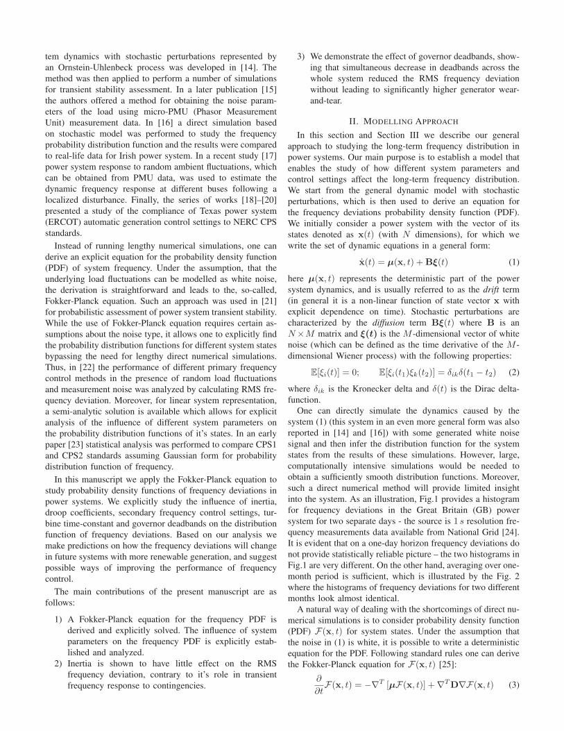
parameters. Fig. 13 illustrates the influence of inertia value

on the frequency PDF for the full nonlinear model. We note,

that in this case the effect is even smaller, than the simplified

linear model gives - lowering inertia from H = 6 s to H = 2s changed the RMS frequency deviation by less than 1 mHz.

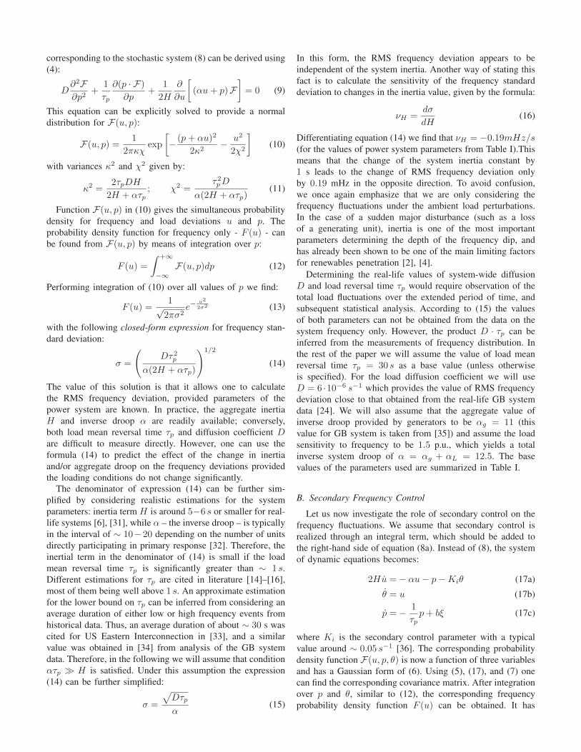
Let us now consider the effect of the system loading level on

the frequency PDF. We use the actual equilibrium loading level

as a base power. Assuming that the relative load fluctuations

TABLE IIVALUES OF INERTIA, INVERSE DROOP, AND TURBINE TIME-CONSTANT

FOR FOUR GENERATORS FOR THE SYSTEM OF FIG. 11 FOR VARIED

SETTINGS

Generator H(s) αg (pu) τT (s)

1 8 13 2

2 10 12 1.75

3 4 10 1.25

4 2 9 1

TABLE IIIVALUES OF LOAD MEAN REVERSAL TIME AND DIFFUSION COEFFICIENTS

FOR TWO LOADS FOR THE SYSTEM OF FIG. 11 FOR VARIED SETTINGS

Load τp (s) D(s−1)

1 25 7.2 · 10−6

2 35 5.1 · 10−6

∆ω (mHz)

-250 -200 -150 -100 -50 0 50 100 150 200 250

Num

ber

of S

am

ple

s

0

500

1000

1500

2000

2500

3000

3500

4000

4500

H = 6s

H = 2s

Fig. 13. Frequency PDF for power system of Fig. 11 obtained fromsimulations over non-linear model for different values of inertia - H = 6s (blue) and H = 2 s (brown).

magnitude is independent of the loading level, all the values

for τp and D stay unchanged in per unit. However, the inverse

droop is proportional to the generator rating rather than the

equilibrium loading level (used as a base power), therefore, a

reduction in the latter effectively corresponds to an increase in

the per unit droop response, unless generating units are being

brought off-line in response to load decrease, thus reducing the

aggregate response. Similarly, since inertia time constant H is

related to base power, reducing the loading level also results in

an increase in total system inertia. The impact of changing the

loading level on the frequency PDF is shown by Fig. 14, with

histograms of the loading levels of 100% and 70%. The lower

loading results in a narrower histogram, and leads to smaller

RMS frequency deviation (51 mHz vs 67 mHz). However, as

was mentioned before, this is only true under the assumption

that all the generating units stay online with the same droop

settings despite the reduction in overall loading level.

V. CONCLUSIONS

We have studied the power system frequency distribution in

the presence of ambient load fluctuations. We considered the

effects of different system parameters on the standard devia-

tion of frequency; the following results can be summarized:

1) Role of inertia and turbine time constant. Under the

assumption (confirmed by real-life data) that the mean

load reversal time τp is at least few decades of seconds,

∆ω (mHz)

-250 -200 -150 -100 -50 0 50 100 150 200 250

Num

ber

of S

am

ple

s

0

500

1000

1500

2000

2500

3000

3500

4000

4500

Part Load

Full Load

Fig. 14. Frequency PDF for power system of Fig. 11 obtained fromsimulations over non-linear model with different loading levels: blue - 100%load, brown - 70% load.

both inertia and turbine time constants have minimal

impact on the frequency standard deviation. This is in

contrast to the case of frequency response to major

contingencies, where exactly these two parameters are of

crucial importance because they determine the size of the

transient frequency dip. On the one hand, this suggests

that reduced system inertia will not cause the increase

of the RMS frequency deviation on it’s own. However,

inertia can be related to some other important parame-

ters, such as aggregate droop. In this case there could be

the correlation between the decrease of inertia and the

increase of the frequency fluctuations (see discussion on

renewables below). Another important conclusion is that

procuring synthetic inertia will not help improving the

RMS frequency deviation and some other measures have

to be taken.

2) Role of governor deadbands. The width of governor

deadbands has a major effect on the frequency dis-

tribution. Frequency tends to spend most of the time

outside the deadband region, regardless of its width.

This suggests that there does not exist any ”optimal”

deadband size, that could substantially reduce wear-and-

tear of generator equipment due to its movement. The

presence of deadbands results in a bi-modal frequency

distribution, which is in excellent agreement with real-

life frequency data from a number of systems [16], [24],

[39].

3) Role of aggregated droop. The aggregate system droop is

the major parameter determining the standard frequency

deviation (eq.(15)). Increasing renewable penetration,

and the corresponding displacement of conventional

generators, can lead to a reduction in the aggregate

system inverse droop α, which will, correspondingly,

cause larger frequency deviations. One of the ways to

deal with the problem is to increase the inverse droop

coefficients of the remaining generators; however, this

could be limited by stability considerations. Use of

energy storage for frequency control could be a solution,

since storage can potentially provide almost deadband-

less and delay-less frequency response [34].

4) Role of renewables penetration. Renewable generation

can bring a number of simultaneous effects to power

system. Reduction of the system inertia is usually cited

as the major one, however, renewable generation could

also increase the effective load diffusion coefficient D,

as well as decreasing the system-wide inverse droop due

to some conventional generation being brought offline

and assuming renewable generators do not participate in

frequency response. Overall, the increased penetration

of renewable sources can lead to substantial increase

of the RMS frequency deviation. According to our

results this problem can not be resolved by procuring

synthetic inertia. The latter can greatly improve the sys-

tem transient response following major contingencies,

but will have minimal effect on the ambient frequency

fluctuations, so that some additional measures have to be

taken. Demanding renewables participation in frequency

response on a continuous basis could be one of such

measures.

REFERENCES

[1] J. Machowski, J. Bialek, and J. Bumby, Power system dynamics: stability

and control. John Wiley & Sons, 2011.[2] J. O’Sullivan, A. Rogers, D. Flynn, P. Smith, A. Mullane, and

M. O’Malley, “Studying the maximum instantaneous non-synchronousgeneration in an island systemfrequency stability challenges in ireland,”IEEE Trans. Power Syst., vol. 29, no. 6, pp. 2943–2951, 2014.

[3] G. Lalor, J. Ritchie, S. Rourke, D. Flynn, and M. J. O’Malley, “Dy-namic frequency control with increasing wind generation,” in Power

Engineering Society General Meeting, 2004. IEEE. IEEE, 2004, pp.1715–1720.

[4] S. Puschel-L, P. Mancarella et al., “Mapping the frequency responseadequacy of the australian national electricity market,” in Universities

Power Engineering Conference (AUPEC), 2017 Australasian. IEEE,2017, pp. 1–6.

[5] F. Teng, V. Trovato, and G. Strbac, “Stochastic scheduling with inertia-dependent fast frequency response requirements,” IEEE Trans. Power

Syst., vol. 31, no. 2, pp. 1557–1566, 2016.[6] A. Ulbig, T. S. Borsche, and G. Andersson, “Impact of low rotational

inertia on power system stability and operation,” IFAC Proceedings

Volumes, vol. 47, no. 3, pp. 7290–7297, 2014.[7] S. EirGrid, “All island tso facilitation of renewables studies,” Eirgrid,

SONI, Dublin, 2010.[8] P. Tielens and D. Van Hertem, “The relevance of inertia in power

systems,” Renewable and Sustainable Energy Reviews, vol. 55, pp. 999–1009, 2016.

[9] R. G. De Almeida and J. P. Lopes, “Participation of doubly fed inductionwind generators in system frequency regulation,” IEEE Trans. Power

Syst., vol. 22, no. 3, pp. 944–950, 2007.[10] D. Gautam, L. Goel, R. Ayyanar, V. Vittal, and T. Harbour, “Control

strategy to mitigate the impact of reduced inertia due to doubly fedinduction generators on large power systems,” IEEE Trans. Power Syst.,vol. 26, no. 1, pp. 214–224, 2011.

[11] F. Teng and G. Strbac, “Evaluation of synthetic inertia provision fromwind plants,” in Power & Energy Society General Meeting, 2015 IEEE.IEEE, 2015, pp. 1–5.

[12] N. Jaleeli and L. S. VanSlyck, “Nerc’s new control performance stan-dards,” IEEE Trans. Power Syst., vol. 14, no. 3, pp. 1092–1099, 1999.

[13] Nerc: Balancing and frequency control. [Online]. Avail-able: https://www.nerc.com/docs/oc/rs/NERC%20Balancing%20and%20Frequency%20Control%20040520111.pdf

[14] F. Milano and R. Zarate-Minano, “A systematic method to model powersystems as stochastic differential algebraic equations,” IEEE Trans.

Power Syst., vol. 28, no. 4, pp. 4537–4544, 2013.[15] C. Roberts, E. M. Stewart, and F. Milano, “Validation of the ornstein-

uhlenbeck process for load modeling based on µpmu measurements,” inPower Systems Computation Conference (PSCC), 2016. IEEE, 2016,pp. 1–7.

[16] F. M. Mele, A. Ortega, R. Zarate-Minano, and F. Milano, “Impactof variability, uncertainty and frequency regulation on power systemfrequency distribution,” in Power Systems Computation Conference

(PSCC), 2016. IEEE, 2016, pp. 1–8.[17] P. Huynh, H. Zhu, Q. Chen, and A. Elbanna, “Data-driven estimation of

frequency response from ambient synchrophasor measurements,” IEEE

Trans. Power Syst., 2018.

[18] H. Chavez, R. Baldick, and S. Sharma, “Regulation adequacy analysisunder high wind penetration scenarios in ercot nodal,” IEEE Trans.

Sustainable Energy, vol. 3, no. 4, pp. 743–750, 2012.[19] H. Chavez, R. Baldick, and J. Matevosyan, “Cps1 compliance-

constrained agc gain determination for a single-balancing authority,”IEEE Trans. Power Syst., vol. 29, no. 3, pp. 1481–1488, 2014.

[20] H. Chvez, R. Baldick, and J. Matevosyan, “The joint adequacy of agcand primary frequency response in single balancing authority systems,”IEEE Trans. on Sustainable Energy, vol. 6, no. 3, pp. 959–966, 2015.

[21] K. Wang and M. L. Crow, “The fokker-planck equation for power systemstability probability density function evolution,” IEEE Trans. Power

Syst., vol. 28, no. 3, pp. 2994–3001, 2013.[22] E. Mallada, “idroop: A dynamic droop controller to decouple power

grid’s steady-state and dynamic performance,” in Decision and Control

(CDC), 2016 IEEE 55th Conference on. IEEE, 2016, pp. 4957–4964.[23] T. Sasaki and K. Enomoto, “Statistical and dynamic analysis of gener-

ation control performance standards,” IEEE Trans. Power Syst., vol. 17,no. 2, pp. 476–481, 2002.

[24] “National grid. frequency data for 2016.” [Online]. Available: https://www.nationalgrid.com/uk/electricity/balancing-services/frequency-response-services/firm-frequency-response?market-information

[25] H. Risken, the Fokker-Plnack Equation: Methods of Solution and Ap-

plications. New York: Springer, 1989.[26] F. Paganini and E. Mallada, “Global performance metrics for synchro-

nization of heterogeneously rated power systems: The role of machinemodels and inertia,” arXiv preprint arXiv:1710.07195, 2017.

[27] J. O’Sullivan, M. Power, M. Flynn, and M. O’Malley, “Modelling offrequency control in an island system,” in Power Engineering Society

1999 Winter Meeting, IEEE, vol. 1. IEEE, 1999, pp. 574–579.[28] G. Lalor, J. Ritchie, D. Flynn, and M. J. O’Malley, “The impact of

combined-cycle gas turbine short-term dynamics on frequency control,”IEEE Trans. Power Syst., vol. 20, no. 3, pp. 1456–1464, 2005.

[29] B. Øksendal, “Stochastic differential equations,” in Stochastic differen-

tial equations. Springer, 2003, pp. 65–84.[30] G. Ghanavati, P. D. Hines, and T. I. Lakoba, “Identifying useful statis-

tical indicators of proximity to instability in stochastic power systems,”IEEE Trans. Power Syst., vol. 31, no. 2, pp. 1360–1368, 2016.

[31] P. M. Ashton, C. S. Saunders, G. A. Taylor, A. M. Carter, and M. E.Bradley, “Inertia estimation of the gb power system using synchrophasormeasurements,” IEEE Trans. Power Syst., vol. 30, no. 2, pp. 701–709,2015.

[32] F. Teng and G. Strbac, “Assessment of the role and value of frequencyresponse support from wind plants,” IEEE Trans. Sustainable Energy,vol. 7, no. 2, pp. 586–595, 2016.

[33] Nerc load-generation and reserves reliability control standards project.[Online]. Available: https://www.energy.gov/sites/prod/files/2016/06/f32/20.%20Martinez%20Load%20Generating%20Reserves.pdf

[34] D. Greenwood, K. Y. Lim, C. Patsios, P. Lyons, Y. S. Lim, and P. Taylor,“Frequency response services designed for energy storage,” Applied

Energy, vol. 203, pp. 115–127, 2017.[35] J. B. Ekanayake, N. Jenkins, and G. Strbac, “Frequency response from

wind turbines,” Wind Engineering, vol. 32, no. 6, pp. 573–586, 2008.[36] P. Kundur, N. J. Balu, and M. G. Lauby, Power system stability and

control. McGraw-hill New York, 1994, vol. 7.[37] P. Pourbeik et al., “Dynamic models for turbine-governors in power

system studies,” IEEE Task Force on Turbine-Governor Modeling, no.2013, 2013.

[38] Y. G. Rebours, D. S. Kirschen, M. Trotignon, and S. Rossignol,“A survey of frequency and voltage control ancillary servicespart i:Technical features,” IEEE Trans. Power Syst., vol. 22, no. 1, pp. 350–357, 2007.

[39] I. Abdur-Rahman, “Frequency regulation: is your plant compliant?introducing wind and solar into the grid highlights the importanceof optimizing power plant frequency regulation capabilities,” Power

Engineering, vol. 114, no. 10, pp. 66–73, 2010.[40] B. Polajzer, D. Dolinar, and J. Ritonja, “Analysis of ace target level for

evaluation of load frequency control performance,” in Energy Conference

(ENERGYCON), 2016 IEEE International. IEEE, 2016, pp. 1–4.[41] “Entso-e supporting document for the network code on load-frequency

control and reserves, june 2013.” [Online]. Available: https://www.

acer.europa.eu/Official documents/Acts of the Agency/Annexes/ENTSO-E%E2%80%99s%20supporting%20document%20to%20the%20submitted%20Network%20Code%20on%20Load-Frequency%20Control%20and%20Reserves.pdf

[42] J. H. Chow and K. W. Cheung, “A toolbox for power system dynamicsand control engineering education and research,” IEEE transactions on

Power Systems, vol. 7, no. 4, pp. 1559–1564, 1992.

Petr Vorobev (M‘15) received his Ph.D. degree intheoretical physics from Landau Institute for Theo-retical Physics, Moscow, in 2010. Currently, he isan Assistant Professor at Skolkovo Institute of Sci-ence and Technology (Skoltech), Moscow, Russia.Before joining Skoltech, he was a Postdoctoral As-sociate at the Mechanical Engineering Departmentof Massachusetts Institute of Technology (MIT),Cambridge. His research interests include a broadrange of topics related to power system dynamicsand control. This covers low frequency oscillations

in power systems, dynamics of power system components, multi-timescaleapproaches to power system modelling, development of plug-and-play controlarchitectures for microgrids.

David M. Greenwood (M14) received the M.Eng.degree in new and renewable energy from DurhamUniversity, Durham, U.K., in 2010 and the Ph.D.degree, for work on real-rime thermal ratings, fromNewcastle University, Newcastle upon Tyne, U.K.,in 2014. He is currently a Senior Research Associateat Newcastle University. His research focusses onflexibility services the role of energy storage withinthe power system.

John H. Bell received his S.B. degree in mechani-cal engineering from the Massachusetts Institute ofTechnology (MIT), Cambridge, in 2018. Currently,he is a masters student in the Mechanical Engineer-ing Department of MIT. His current research inter-ests primarily consist of the dynamics, control, anddesign of robotic and electromechanical systems.This covers topics such as motor control, gait controlfor legged robots, and coordination of compoundrobot-human systems.

Janusz W. Bialek (F11) received M.Eng. (1977)and Ph.D. (1981) degrees from Warsaw Universityof Technology, Warsaw, Poland. He is FoundingDirector of the Center for Energy Systems, SkolkovoInstitute of Science and Technology (Skoltech), Rus-sia, having previously held Chair positions at TheUniversity of Edinburgh (20032009), and DurhamUniversity (20092014). His interests are in smartgrids, energy system integration, power system dy-namics, power system control, power system eco-nomics, and preventing electricity blackouts.

Philip C. Taylor (SM12) received the Engineer-ing Doctorate in the field of intelligent demandside management techniques from the Universityof Manchester Institute of Science and Technology(UMIST), Manchester, U.K., in 2001. He joinedNewcastle University, Newcastle upon-Tyne, U.K.,in April 2013 where he is the Head of the School ofEngineering and holds the Siemens Chair of EnergySystems. He is a visiting Professor at Nanyang Tech-nological University in Singapore and he previouslyheld the DONG Energy Chair in Renewable Energy

and was a Director of the Durham Energy Institute.

Konstantin Turitsyn (M‘09) received the M.Sc.degree in physics from Moscow Institute of Physicsand Technology and the Ph.D. degree in physicsfrom Landau Institute for Theoretical Physics,Moscow, in 2007. He was an Associate Profes-sor at the Mechanical Engineering Department ofMassachusetts Institute of Technology (MIT), Cam-bridge. Before joining MIT, he held the position ofOppenheimer fellow at Los Alamos National Lab-oratory, and KadanoffRice Postdoctoral Scholar atUniversity of Chicago. His research interests encom-

pass a broad range of problems involving nonlinear and stochastic dynamicsof complex systems. Specific interests in energy related fields include stabilityand security assessment, integration of distributed and renewable generation.