De Luca, F., Verderame, G., & Manfredi, G. (2015). Analytical versusobservational fragilities:: the case of Pettino (L’Aquila) damage datadatabase. Bulletin of Earthquake Engineering, 13(4), 1161-1181. DOI:10.1007/s10518-014-9658-1

Peer reviewed version

Link to published version (if available):10.1007/s10518-014-9658-1

Link to publication record in Explore Bristol ResearchPDF-document

University of Bristol - Explore Bristol ResearchGeneral rights

This document is made available in accordance with publisher policies. Please cite only the publishedversion using the reference above. Full terms of use are available:http://www.bristol.ac.uk/pure/about/ebr-terms

1

Analytical versus observational fragilities: the case

of Pettino (L’Aquila) damage data database

De Luca Flavia, Verderame Gerardo M.* , Manfredi G.

Università degli Studi di Napoli Federico II, DiSt, Via Claudio 21, 80125 Napoli

Abstract

A damage data database of 131 reinforced concrete (RC) buildings, collected after 2009 L’Aquila

(Italy) earthquake, is employed for the evaluation of observational fragility curves. The specific

interpretation of damage data allowed carrying out fragility curves for slight, moderate, and

heavy damage, (i.e., DS1, DS2, and DS3), defined according to EMS 98 macroseismic scale.

Observational fragility curves are then employed for the calibration of FAST analytical

methodology. FAST method is a spectral based approach, meant for the estimate of fragility

curves of infilled RC buildings up to DS3, evaluated, again, according to EMS98. Kullback-

Leibler divergence is employed to check the matching between analytical and observational

fragilities. FAST input variables can vary in quite large ranges and the calibration provides a

valuable suggestion for the application of the method in other cases in which field damage data

are not available. Results showed that optimizing values, for the input variables calibrated, are in

good agreement with typical values assumed in literature. Analytical results showed a very

satisfactory agreement with observational data for DS2 and DS3, while systematical

underestimation was found for the case of DS1.

Keywords: L’Aquila earthquake, EMS98, observational fragilities, FAST method, infills.

1. INTRODUCTION

Usability and damage data collected after earthquakes represent a key tool for validation of

analytical vulnerability procedures. Herein, a database of 131 reinforced concrete (RC) buildings

collected after 2009 L’Aquila earthquake, in the neighborhood of Pettino, is employed to carry out

observational fragility curves for Slight, Moderate and Heavy damage states classified according

to EMS 98 (Grünthal et al. 1998). Other than being available outcomes of official usability

inspections collected by Italian National Civil Protection right after the event, further data (e.g.,

transversal and longitudinal dimensions in plan), on the population of buildings, were collected

during independent field surveys (Polidoro, 2010). Notwithstanding the fact that the population is

not so large (131 buildings), the combination of the two sources of information resulted in a quite

accurate database.

Observational fragility curves, carried out in this study, are in good agreement with other

vulnerability results available in literature for the same earthquake (Liel and Lynch 2012), and

based on a larger database. The observational fragilities obtained are then employed for the

calibration of FAST method, a large scale vulnerability approach for infilled RC moment resisting

frames (MRF). This methodology has been applied to different earthquake cases (De Luca et al.

2013a; Manfredi et al. 2013), such as Lorca (2011), Spain, and Emilia (2012), Italy. The approach

belongs to the wider family of vulnerability assessment methodologies based on spectral

displacements (e.g., Kircher et al. 1997; Erdik et al. 2004, among others) in which damage states

are classified according to the 1998 European Macroseismic Scale (Grünthal et al. 1998). On the

other hand, in analogy with other vulnerability approaches available in literature (e.g., Ricci 2010),

it is able to capture the structural contribution provided by nonstructural masonry infills. The latter

represent a key aspect of the method; in fact, recent reconnaissance reports after earthquakes in the

Mediterranean area (e.g., Sezen et al. 2003; Decanini et al. 2004; Ricci et al. 2011a) emphasized

that infills provide a first source of capacity for RC MRF frames. On the other hand, infills’

stiffness contribution often results in a localization of damage at lower storeys (e.g., Ricci et al.

* Corresponding author: verderam@unina.it

2

2013), and local interaction between RC elements and masonry infills can lead to undesirable

brittle failures in the elements (e.g., Vederame et al. 2011). Notwithstanding the fact that FAST

method is not able to capture damage states resulting from brittle failures in RC elements because

of local interaction with masonry infills or because of lack of detailing in transversal

reinforcement; it represents a very straightforward and easy-to-apply approach aimed at capturing

damage states from slight to heavy.

Even if comparisons of FAST with damage data have been made also for Lorca and Emilia

earthquakes (see De Luca et al. 2013a; Manfredi et al. 2013), this is the first case in which damage

data are enough accurate to carry out observational fragility curves to be compared to FAST

analytical fragilities. Thus, it was possible to calibrate input variables of FAST method and select

the optimal choice to get a satisfactory agreement between observational and analytical data.

Optimal variables leading to the best matching between observational results are selected

assuming the Kullback-Leibler divergence (Kullback and Liebler 1951) as measure of

optimization.

Section 2 provides a description of the database and of the hypotheses made to carry out

observational fragilities. Section 3 describes the basis of FAST method and uncertainties

considered for analytical fragility curves. Finally, section 4 and section 5 provide results of the

calibration and main conclusions of this study.

2. PETTINO (L’AQUILA) DAMAGE DATA DATABASE

The database considered in this study is made of 131 infilled RC MRF frames located in

Pettino neighborhood in L’Aquila. Pettino area was very close to the epicenter of the mainshock

event of L’Aquila 2009 earthquake. The 131 buildings are selected according to data collected

from the official post-earthquake inspection forms by Italian National Civil Protection (Polidoro

2010). The 131 buildings are (i) RC buildings, (ii) regular in plan and elevation, and (iii)

characterized by regular distribution of the infills.

In the following, a brief overview of earthquake characteristics and a description of database

characteristics are provided. This information are then employed for the evaluation of

observational fragilities according to the methodology employed by Liel and Lynch (2012), and

described in Porter et al. (2007).

2.1 L’Aquila earthquake

On 6th April 2009, an earthquake of magnitude Mw=6.3 struck the Abruzzo region; the

epicenter was only about 6 km from the city of L’Aquila. The event resulted in casualties and

damage to buildings, lifelines and other infrastructures. The closest stations to the epicenter were

located on the fault trace (AQA, AQV, AQK, AQG). The maximum Peak Ground Acceleration

(PGA) registered was 613.8 cm/s2 on the East-West component of AQV station, whose soil type

was classified according to cross-hole test as type B (Chioccarelli et al. 2009).

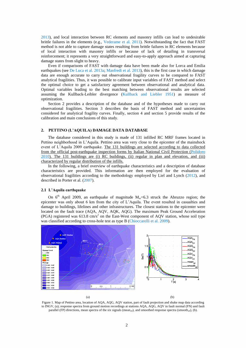
(a) (b)

Figure 1. Map of Pettino area, location of AQA, AQG, AQV station, part of fault projection and shake map data according

to INGV, (a); response spectra from ground motion recordings at stations AQA, AQG, AQV in fault normal (FN) and fault

parallel (FP) directions, mean spectra of the six signals (meanall), and smoothed response spectra (smoothall), (b).

3

The database of 131 buildings is located in Pettino, a neighborhood of L’Aquila. Pettino is

very close to three stations (AQA, AQG, AQV), see Figure 1a. The three stations are located in the

epicentral area and part of Pettino is located within fault projection. In Figure 1b response spectra

from ground motion recordings at stations AQA, AQG and AQV are shown. Recorded signal have

been rotated from North-South (NS) and East-West (EW) (original directions of the

accelerometers) to strike-normal (FN) and strike-parallel (FP) components. Notwithstanding

different evaluations of strike angle available in literature for 2009 L’Aquila earthquake (e.g.,

Walters et al. 2009), strike angle was assumed equal to 127°, according to the evaluation provided

by Istituto Nazionale di Geofisica e Vulcanologia, INGV, (http://itaca.mi.ingv.it/ItacaNet/).

Mean PGA value of the six signals is equal to 0.476g. A smoothed spectrum (smoothall in

Figure 1b), evaluated from the mean spectra of the six signals (meanall in Figure 1b), was

computed through the procedure provided in Malhotra (2006). The smoothed spectrum allows

identifying values of TC and TD for the smoothed Newmark-Hall spectral shape. TC represents the

right bound period of the constant acceleration branch, while TD is the right bound period of

constant velocity branch. TC and TD are equal, respectively to 0.42s and 0.97s.

2.2 Database description and EMS98 classification

The database considered in this study is made of 131 RC buildings, located in the area of

Pettino. These buildings have been inspected after 2009 L’Aquila earthquake; in particular, the

population has been divided in three bins (BIN 1, BIN 2, and BIN 3), defined according two main

criteria. First criterion is a different average PGA characterizing each BIN, second criterion is that

each BIN has approximately the same number of buildings, (see Figure 1a).

The database was assembled through fieldwork (Polidoro 2010) and collection of data

available from official inspection forms (Baggio et al. 2000).

The official Italian inspection form, the so-called AeDES† form, conjugates safety evaluation

and damage assessment (Baggio et al. 2000; Goretti and Di Pasquale 2006). The Italian AeDES

form is made of nine sections. In section 1 are collected all the necessary information for the

identification of the building (e.g., city, municipality, street address). In section 2 general building

information are collected (e.g., number of storeys, interstorey height, average surface in plan, age

of construction). In section 3, building typology (RC, steel, masonry) is identified, and lateral (e.g.,

frame, wall) and horizontal structural systems are classified. Furthermore, in section 3, information

about regularity in elevation and in plan because of the structural system and because of masonry

infills are collected. Section 4 provides damage evaluation for structural components and infill

walls, as it will be discussed above. Section 5 provides information about damage to non-structural

elements (e.g., plaster, chimneys,…), section 6 collects information about danger for usability

caused by adjacent structures, and section 7 is focused on foundations and soil. Finally, section 8

collects risk evaluation and the final outcome of the usability survey, with the possibility to add

further information in section 9. A detailed description of the form is provided in the field manual

by Baggio et al. (2000).

(a) (b) (c)

Figure 2. Examples of damage to infills in the area of Pettino

†Available at http://www.protezionecivile.gov.it/resources/cms/documents/Scheda_AEDES.pdf

4

A further selection with respect to data of Polidoro is made: buildings selected are

approximately rectangular in plan, and they are characterized by approximately regular

distribution of infills in elevation. Database includes each building’s location, street address, area

in plan, and a rough estimation of transversal and longitudinal dimensions. The latter information

(transversal and longitudinal dimensions) is not available in the inspection form, and it was

collected through fieldwork in loco, and further controls were made through Google Maps ®.

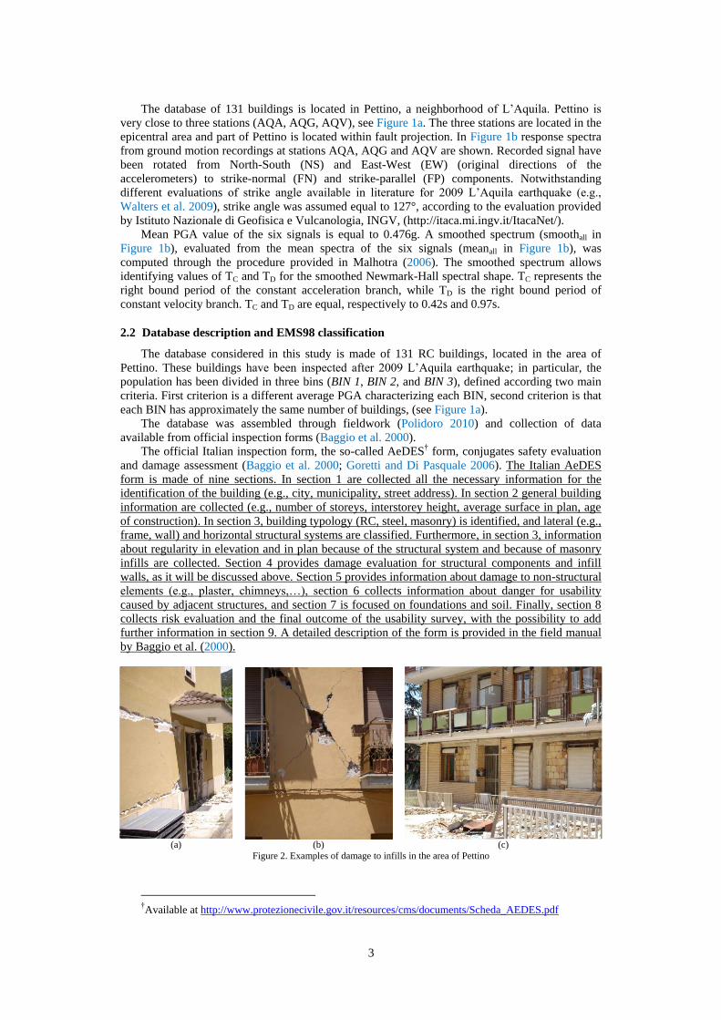
Figure 2 shows some examples of RC buildings in the area of Pettino.

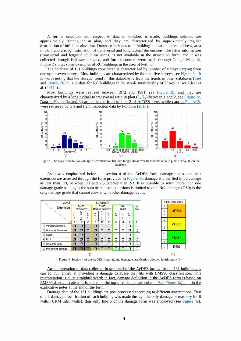
The database of 131 buildings considered is characterized by number of storeys varying from

one up to seven storeys. Most buildings are characterized by three to five storeys, see Figure 3a. It

is worth noting that the storeys’ trend in this database reflects the trends in other databases (Liel

and Lynch, 2012), and data for RC buildings in the whole municipality of L’Aquila, see Ricci et

al. (2011a).

Most buildings were realized between 1972 and 1991, see Figure 3b, and they are

characterized by a longitudinal to transversal ratio in plan (Lx/Ly) between 1 and 2, see Figure 3c.

Data in Figure 3a and 3b are collected from section 2 of AeDES form, while data in Figure 3c

were retrieved by Gis and field inspection data by Polidoro (2010).

(a) (b) (c)

Figure 3. Storeys’ distribution (a), age of construction (b), and longitudinal over transversal ratio in plan, Lx/Ly, (c) in the

database.

As it was emphasized before, in section 4 of the AeDES form, damage states and their

extension are assessed through the form provided in Figure 4a; damage is classified in percentage

as less than 1/3, between 1/3 and 2/3, greater than 2/3. It is possible to select more than one

damage grade as long as the sum of relative extensions is limited to one. Null damage (DS0) is the

only damage grade that cannot coexist with other damage levels.

(a) (b)

Figure 4. Section 4 of the AeDES from (a), and damage classification adopted in this study (b).

An interpretation of data collected in section 4 of the AeDES forms, for the 131 buildings, is

carried out, aimed at providing a damage database that fits with EMS98 classification. This

interpretation is quite straightforward; in fact, damage definition in the AeDES form is based on

EMS98 damage scale as it is stated on the top of each damage column (see Figure 4a), and in the

explicative notes at the end of the form.

Damage data of the 131 buildings are post processed according to different assumptions. First

of all, damage classification of each building was made through the only damage of masonry infill

walls (URM infill walls), thus only line 5 of the damage form was employed (see Figure 4a).

URM infill walls

A

≥DS3B

C

D

≥DS2E

F

G

≥DS1H

I

L DS0

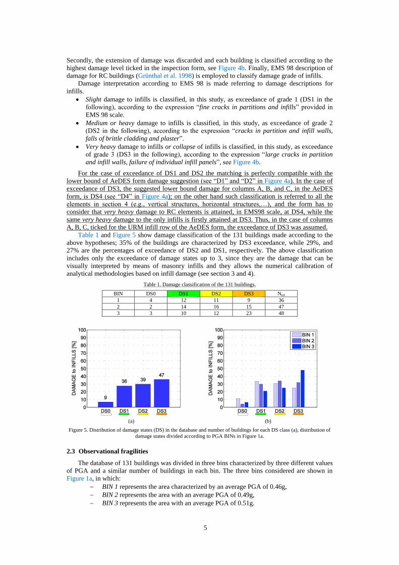
5

Secondly, the extension of damage was discarded and each building is classified according to the

highest damage level ticked in the inspection form, see Figure 4b. Finally, EMS 98 description of

damage for RC buildings (Grünthal et al. 1998) is employed to classify damage grade of infills.

Damage interpretation according to EMS 98 is made referring to damage descriptions for

infills.

Slight damage to infills is classified, in this study, as exceedance of grade 1 (DS1 in the

following), according to the expression “fine cracks in partitions and infills” provided in

EMS 98 scale.

Medium or heavy damage to infills is classified, in this study, as exceedance of grade 2

(DS2 in the following), according to the expression “cracks in partition and infill walls,

falls of brittle cladding and plaster”.

Very heavy damage to infills or collapse of infills is classified, in this study, as exceedance

of grade 3 (DS3 in the following), according to the expression “large cracks in partition

and infill walls, failure of individual infill panels”, see Figure 4b.

For the case of exceedance of DS1 and DS2 the matching is perfectly compatible with the

lower bound of AeDES form damage suggestion (see “D1” and “D2” in Figure 4a). In the case of

exceedance of DS3, the suggested lower bound damage for columns A, B, and C, in the AeDES

form, is DS4 (see “D4” in Figure 4a); on the other hand such classification is referred to all the

elements in section 4 (e.g., vertical structures, horizontal structures,…), and the form has to

consider that very heavy damage to RC elements is attained, in EMS98 scale, at DS4, while the

same very heavy damage to the only infills is firstly attained at DS3. Thus, in the case of columns

A, B, C, ticked for the URM infill row of the AeDES form, the exceedance of DS3 was assumed.

Table 1 and Figure 5 show damage classification of the 131 buildings made according to the

above hypotheses; 35% of the buildings are characterized by DS3 exceedance, while 29%, and

27% are the percentages of exceedance of DS2 and DS1, respectively. The above classification

includes only the exceedance of damage states up to 3, since they are the damage that can be

visually interpreted by means of masonry infills and they allows the numerical calibration of

analytical methodologies based on infill damage (see section 3 and 4).

Table 1. Damage classification of the 131 buildings.

BIN DS0 DS1 DS2 DS3 Ntot

1 4 12 11 9 36

2 2 14 16 15 47

3 3 10 12 23 48

(a) (b)

Figure 5. Distribution of damage states (DS) in the database and number of buildings for each DS class (a), distribution of

damage states divided according to PGA BINs in Figure 1a.

2.3 Observational fragilities

The database of 131 buildings was divided in three bins characterized by three different values

of PGA and a similar number of buildings in each bin. The three bins considered are shown in

Figure 1a, in which:

BIN 1 represents the area characterized by an average PGA of 0.46g,

BIN 2 represents the area with an average PGA of 0.49g,

BIN 3 represents the area with an average PGA of 0.51g.

6

The average PGA of each BIN was extrapolated from the shake map provided by INGV

(http://shakemap.rm.ingv.it/shake/index.html). The shake map in the area of Pettino has been

downscaled according to the PGA ranges provided in Figure 1a; then after the three BINs have

been defined, the weighted mean PGAs for each bin have been evaluated taking into account the

location of the buildings in each bin.

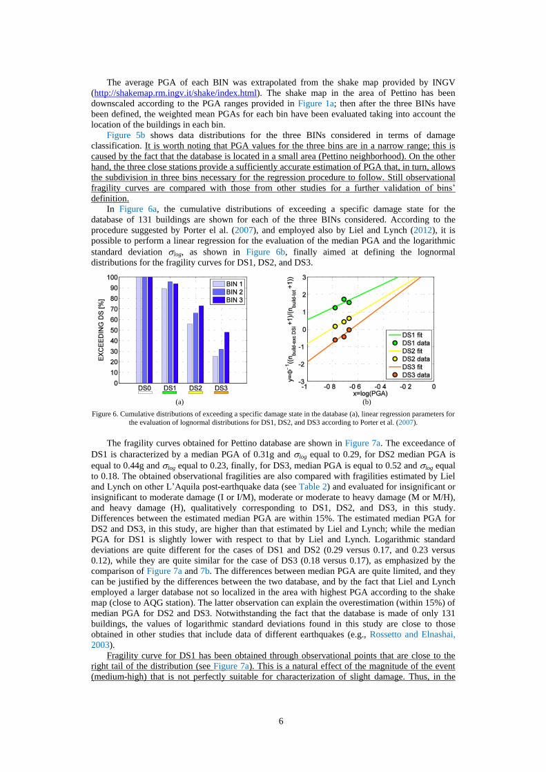
Figure 5b shows data distributions for the three BINs considered in terms of damage

classification. It is worth noting that PGA values for the three bins are in a narrow range; this is

caused by the fact that the database is located in a small area (Pettino neighborhood). On the other

hand, the three close stations provide a sufficiently accurate estimation of PGA that, in turn, allows

the subdivision in three bins necessary for the regression procedure to follow. Still observational

fragility curves are compared with those from other studies for a further validation of bins’

definition.

In Figure 6a, the cumulative distributions of exceeding a specific damage state for the

database of 131 buildings are shown for each of the three BINs considered. According to the

procedure suggested by Porter el al. (2007), and employed also by Liel and Lynch (2012), it is

possible to perform a linear regression for the evaluation of the median PGA and the logarithmic

standard deviation log, as shown in Figure 6b, finally aimed at defining the lognormal

distributions for the fragility curves for DS1, DS2, and DS3.

(a) (b)

Figure 6. Cumulative distributions of exceeding a specific damage state in the database (a), linear regression parameters for

the evaluation of lognormal distributions for DS1, DS2, and DS3 according to Porter et al. (2007).

The fragility curves obtained for Pettino database are shown in Figure 7a. The exceedance of

DS1 is characterized by a median PGA of 0.31g and log equal to 0.29, for DS2 median PGA is

equal to 0.44g and log equal to 0.23, finally, for DS3, median PGA is equal to 0.52 and log equal

to 0.18. The obtained observational fragilities are also compared with fragilities estimated by Liel

and Lynch on other L’Aquila post-earthquake data (see Table 2) and evaluated for insignificant or

insignificant to moderate damage (I or I/M), moderate or moderate to heavy damage (M or M/H),

and heavy damage (H), qualitatively corresponding to DS1, DS2, and DS3, in this study.

Differences between the estimated median PGA are within 15%. The estimated median PGA for

DS2 and DS3, in this study, are higher than that estimated by Liel and Lynch; while the median

PGA for DS1 is slightly lower with respect to that by Liel and Lynch. Logarithmic standard

deviations are quite different for the cases of DS1 and DS2 (0.29 versus 0.17, and 0.23 versus

0.12), while they are quite similar for the case of DS3 (0.18 versus 0.17), as emphasized by the

comparison of Figure 7a and 7b. The differences between median PGA are quite limited, and they

can be justified by the differences between the two database, and by the fact that Liel and Lynch

employed a larger database not so localized in the area with highest PGA according to the shake

map (close to AQG station). The latter observation can explain the overestimation (within 15%) of

median PGA for DS2 and DS3. Notwithstanding the fact that the database is made of only 131

buildings, the values of logarithmic standard deviations found in this study are close to those

obtained in other studies that include data of different earthquakes (e.g., Rossetto and Elnashai,

2003).

Fragility curve for DS1 has been obtained through observational points that are close to the

right tail of the distribution (see Figure 7a). This is a natural effect of the magnitude of the event

(medium-high) that is not perfectly suitable for characterization of slight damage. Thus, in the

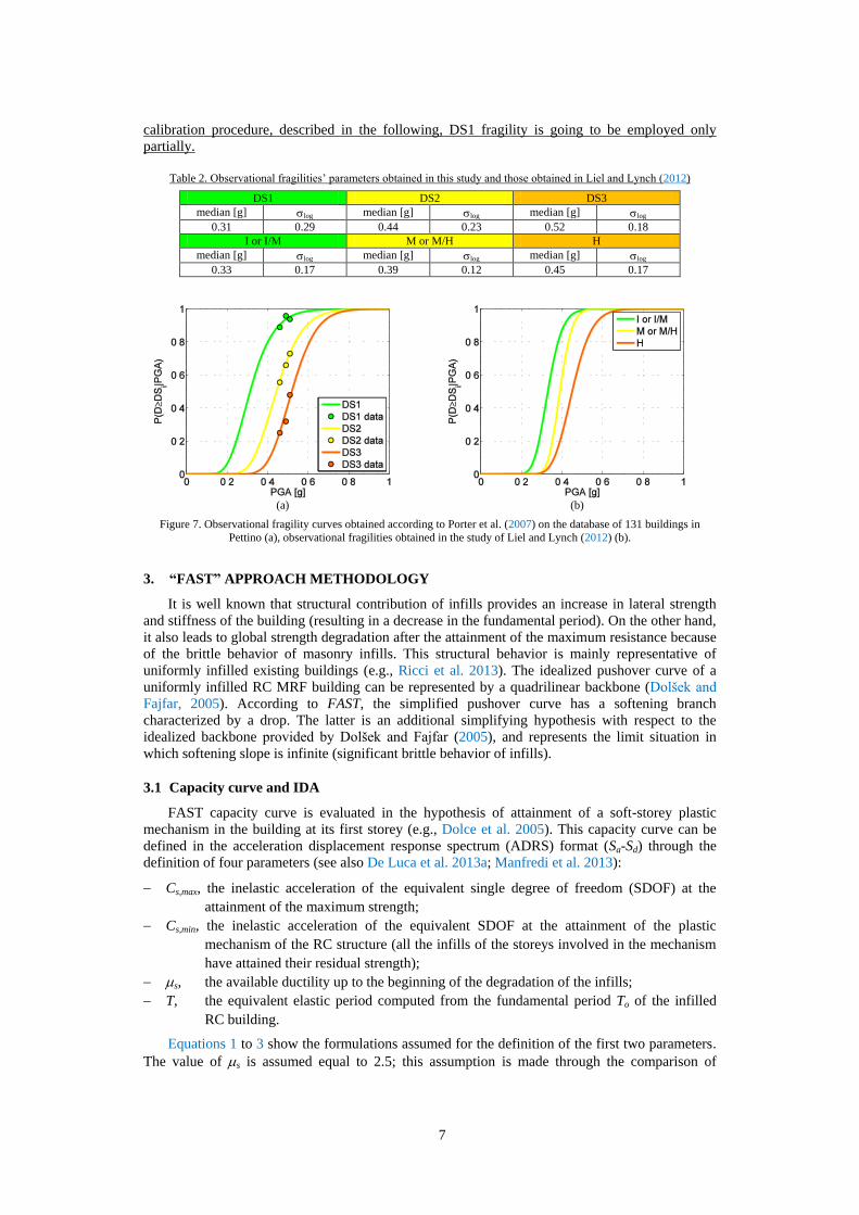
7

calibration procedure, described in the following, DS1 fragility is going to be employed only

partially.

Table 2. Observational fragilities’ parameters obtained in this study and those obtained in Liel and Lynch (2012)

DS1 DS2 DS3

median [g] log median [g] log median [g] log

0.31 0.29 0.44 0.23 0.52 0.18

I or I/M M or M/H H

median [g] log median [g] log median [g] log

0.33 0.17 0.39 0.12 0.45 0.17

(a) (b)

Figure 7. Observational fragility curves obtained according to Porter et al. (2007) on the database of 131 buildings in

Pettino (a), observational fragilities obtained in the study of Liel and Lynch (2012) (b).

3. “FAST” APPROACH METHODOLOGY

It is well known that structural contribution of infills provides an increase in lateral strength

and stiffness of the building (resulting in a decrease in the fundamental period). On the other hand,

it also leads to global strength degradation after the attainment of the maximum resistance because

of the brittle behavior of masonry infills. This structural behavior is mainly representative of

uniformly infilled existing buildings (e.g., Ricci et al. 2013). The idealized pushover curve of a

uniformly infilled RC MRF building can be represented by a quadrilinear backbone (Dolšek and

Fajfar, 2005). According to FAST, the simplified pushover curve has a softening branch

characterized by a drop. The latter is an additional simplifying hypothesis with respect to the

idealized backbone provided by Dolšek and Fajfar (2005), and represents the limit situation in

which softening slope is infinite (significant brittle behavior of infills).

3.1 Capacity curve and IDA

FAST capacity curve is evaluated in the hypothesis of attainment of a soft-storey plastic

mechanism in the building at its first storey (e.g., Dolce et al. 2005). This capacity curve can be

defined in the acceleration displacement response spectrum (ADRS) format (Sa-Sd) through the

definition of four parameters (see also De Luca et al. 2013a; Manfredi et al. 2013):

Cs,max, the inelastic acceleration of the equivalent single degree of freedom (SDOF) at the

attainment of the maximum strength;

Cs,min, the inelastic acceleration of the equivalent SDOF at the attainment of the plastic

mechanism of the RC structure (all the infills of the storeys involved in the mechanism

have attained their residual strength);

s, the available ductility up to the beginning of the degradation of the infills;

T, the equivalent elastic period computed from the fundamental period To of the infilled

RC building.

Equations 1 to 3 show the formulations assumed for the definition of the first two parameters.

The value of s is assumed equal to 2.5; this assumption is made through the comparison of

8

detailed assessment studies available in literature on gravity load designed buildings (Ricci et al.

2013; Verderame et al. 2012a).

max w

s ,max s ,designC C

N m (1)

max w

s ,min s ,designC C

N m (2)

, , ( ) s design a dC S T R R (3)

in which, N is the number of storeys, m is the average mass of each storey normalized by the

building area (e.g., equal to 0.8t/m2 for residential buildings), is a coefficient for the evaluation

of the first mode participant mass with respect to the total mass of the multiple degree of freedom

(MDOF) according to (CEN, 2004), max is the maximum shear stress of the infills according to

Fardis (1997), and equal to 1.30 times the cracking shear stress of the infills (cr), w is the ratio

between the infill area, Aw, (internal+external infills) - evaluated along one of the principal

directions of the building - and the building area Ab.

and are coefficients that account, respectively, for RC elements’ strength contribution at

the attainment of infill peak strength and for the residual strength contribution of the infills at the

attainment of the plastic mechanism of the bare RC structure. Cs,design is the design acceleration

coefficient of the bare structure at the attainment of the plastic mechanism of the bare RC

structure. It can be evaluated made considering obsolete seismic design provisions in terms of

design spectral acceleration, amplified by structural redundancy factor (R) and overstrength

material factor (R), see De Luca et al. (2013a) for details.

Last parameter to be evaluated for the definition of the capacity curve is the equivalent elastic

period T. The first branch of the curve represents both the initial elastic and the post-cracking

behavior occurred in both RC frame and infills. Hence, the equivalent elastic period T of the

idealized capacity curve is higher than the fundamental elastic period T0, correspondent to the

tangent stiffness of the capacity curve. In particular, in this study, T is evaluated through a

relationship with To. In FAST, To is computed through equation 4, (Ricci et al. 2011b), given its

good agreement with experimental data, and the presence of variables already employed in the

evaluation of the simplified capacity curve (see equations 1 and 2). Finally, the switch from T0 to

the equivalent elastic period T is made through the amplification coefficient , calibrated on

analytical data (Manfredi et al. 2012; Verderame et al. 2012a), and equal to 1.40.

0.023 0.0023100

o

w w

H HT

(4)

The simplified capacity curve allows consequent definition of approximate Incremental

Dynamic Analysis curves (IDA or IN2). Capacity curve and approximate IDA curve are related by

an R--T relationship. In the following the R--T relationship, also known as SPO2IDA, by

Vamvatsikos and Cornell (2006), is employed. SPO2IDA provides a relationship between an

engineering demand parameter (EDP), e.g. SDOF displacement (Sd), and an intensity measure

(IM), e.g. elastic spectral acceleration Sa or PGA, and it evaluates record to record variability

providing directly not only median approximate IDA curves but also their 16° and 84° percentiles.

Other FAST applications available in literature (De Luca et al. 2013a; De Luca et al., 2013b;

Manfredi et al. 2013) employed the R--T relationship calibrated on infilled RC buildings by

Dolšek and Fajfar (2004). Both R--Ts provides similar results, and FAST results are not strictly

affected by this choice.

3.2 Damage analysis and seismic capacities

The IDA curve represents the specific building (or building class) relationship between Sd-Sa

of the equivalent SDOF. This relationship allows the transformation of specific displacement

thresholds (for DS1, or DS2, or DS3) in terms of corresponding IM thresholds (in terms of Sa, or

PGA). These IMs values represent the capacity of the structure (or the class of structures) at the

considered DSs in terms of IM. Thus, for the evaluation of the IM capacity, it is firstly necessary

9

to provide an estimation of damage threshold for the specific buildings in terms of spectral

displacement (Sd).

The evaluation of the SDOF displacement corresponding to a specified DS level (Sd|DSi) can be

made through interstorey drift ratios at which the specific DSs are attained (IDR|DSi). DSs in terms

of IDR can be defined through an empirical-mechanical interpretation of damage classification of

the EMS-98 scale (Grünthal et al. 1998). Definition of IDR|DSi is made for the DSs characterized

by a specific definition of infill damage in the EMS98 scale. In particular, such procedure can be

pursued up to DS3:

DS1: fine cracks in partitions and infills. This DS is defined at the end of the phase in

which infills are characterized by an elastic uncracked stiffness. The IDR|DS1 could be

evaluated as the drift characterizing the attainment of the cracking shear in the infill

backbone (Fardis, 1997). Hence, from a mechanical point of view the lateral drift

corresponding to this DS can be defined as the ratio of tangential cracking stress (cr) to the

shear elastic modulus (Gw) of the infills. Considering the values suggested for cr and Gw in

Circolare 617 (02/02//2009) for typical clay hollow bricks employed in Italy, and taking

into account the experimental results in Colangelo (2003; 2012), the range in which IDR|DS1

can vary is [0.02% ÷ 0.1%].

DS2: cracks in partition and infill walls, fall of brittle cladding and plaster. After cracking,

with increasing displacement, a concentration of stresses along the diagonal of the infill

panel takes place, together with an extensive diagonal cracking, up to the attainment of the

maximum resistance. Thus, IDR|DS2 can be assumed at the achievement of maximum

strength in the infills. In a pure mechanical approach, IDR|DS2 could be evaluated as the drift

corresponding to the peak of infill backbone according to Fardis’ model (1997). IDR|DS2

could be assumed in the range [0.2% ÷ 0.4%], whose boundary values are similar,

respectively, to that in Dolšek and Fajfar (2008), and Colangelo (2003; 2012).

DS3: large cracks in partition and infill walls, failure of individual infill panels. At this

stage the generic infill panel shows a significant strength drop with a consequent likely

collapse of the panel. According to Fardis’ backbone, the drift at this stage is strictly

dependent on the softening stiffness of the infill. On the other hand, the softening stiffness

is characterized by a large variability depending on the specific kind of infill (mechanical

properties, type of bricks, etc.). IDR|DS3 could be assumed in the range [0.8% ÷ 1.6%],

whose boundary values are similar respectively to that in Dolšek and Fajfar (2008), and

Colangelo (2003; 2012).

It is worth noting that IDR ranges considered above are characteristic of clay hollow brick

infills, typical in the Mediterranean area, and for which a fair number of experimental tests are

available in literature. Once IDR|DSi is computed, roof displacement ∆|DSi of the MDOF can be

defined through the evaluation of an approximate deformed shape. The switch from roof

displacement ∆|DSi to SDOF displacement Sd|DSi is, then, obtained through the first mode

participation factor1 evaluated according to the tabulated values in ASCE/SEI 41-06 (2007), the

so called coefficient Co (equivalent to 1).

The deformed shape at a given DS level is evaluated according to the following assumptions:

the IDR|DSi is attained at the first storey;

the deformed shape of the (N-1) storeys is evaluated as function of their stiffness with

respect to that expected at the first storey.

In the case of DS1 and DS2, the SDOF displacement Sd|DSi is evaluated according to equation

5 and 6, in which hint is the interstorey height of the building (generally considered equal to 3.0m).

The IDR of the ith (i>1) storey is evaluated considering the inverted triangular distribution of

lateral forces as shown in equation 7, in which Hi and Hj are the heights of the ith and jth storeys

above the level of application of the seismic action (foundation or top of a rigid basement).

Coefficient in equation 5 is the average of the ratio, i=K1/Ki, between the stiffness of the first

storey (K1) and that of the ith storey (Ki); all evaluated considering the only infills’ contribution and

neglecting concrete stiffness contribution at the different storeys.

10

1 2

21

1 N

d|DS , DS int i int

i

S ( IDR h IDR h )

(5)

3 2 int

3 2

1

( )

DS DS

d DS d DS

IDR IDR hS S (6)

1

1

1

(1 )i

i

Ni DS

j

j

HIDR IDR

H

(7)

For DS1, the stiffness of all the storeys is still elastic; hence, is equal to 1.0. For DS2 the

deformed shape is computed considering secant stiffness at the first storey and a combination of

stiffness at the other (N-1) storeys. For DS3, Sd|DS3 is evaluated assuming the same deformed shape

for the (N-1) storeys carried out for DS2. Thus, Sd|DS3 increasing is generated by IDR|DS3, as shown

in equation 7. The latter assumption implies that the unloading stiffness of the (N-1) storeys is

infinite. From a theoretical point of view, can vary in a wide range [0.0 ÷ 1.0]. If =1.0, it means

that each storey has attained the same secant stiffness of the first storey; while in the case of =0

the remaining (N-1) storeys do not provide any contribution to Sd|DS2. In other words, the

coefficient allows evaluating the deformed shape of the remaining (N-1) storeys. In previous

studies it was shown that =0.40 has a fair agreement with observational data (De Luca et al.

2013a; Manfredi et al. 2013; De Luca et al. 2013b).

Sd|DSi for DS1, DS2, and DS3 allows the consequent definition of the spectral acceleration

threshold at a given DS, Sa|DSi through the IDA curve. Given Sa|DSi, the switching to PGA|DSi (i.e.,

PGA threshold at a given DS) is pursued through a spectral scaling procedure. This is the first step

in which it is necessary to assume a spectral shape.

According to data available in each case it is possible to employ a spectral shape from a

recorded accelerograms (De Luca et al. 2013a), or a code spectral shape (Manfredi et al. 2013), or

a smoothed spectral shape (see Figure 1b). The above description of FAST method allows the

definition of the median PGA capacity characterizing the exceedance of DS1, DS2, and DS3 for

infilled RC MRF buildings (PGA|DSi).

An example application of FAST method on a complex model of a single building is provided

in Verderame et al. (2012a) and a comparison with other accurate numerical approaches is

provided.

3.3 Fragility curves and uncertainties

A Monte Carlo simulation, carried out after the definition and characterization of uncertainties

to be considered, allows providing fragility curves through FAST method at the three DS

considered. FAST input variables of the method can be divided in:

variables defining building characteristics (building variables). Building variables are the

number of storeys (N), interstorey height (hint), the ratio between infill area and building

area along a direction (w), and the storey specific mass (m). Such variables depends on

geometrical and usage characteristics of the building;

variables defining the design practice at the time of construction (design variables) for the

area considered, such as the design spectral acceleration Sad(T) or the redundancy factor R

(see equation 3);

variables characterizing material mechanical properties (material variables): such as the

peak shear stress of the infills (max=1.30cr) and the overstrength factor R, mainly

ascribed to the overstrength factor between mean steel yielding strength and design

strength (fym/fd);

variables characterizing damage state thresholds (damage state variables), i.e., IDR|DSi;

variables defining FAST method hypotheses (method variables), i.e., , , , , s.

Notwithstanding the fact that all variables can be characterized by specific uncertainties given

the kind of information available; in the following are described the typical assumption made for

FAST application in this study and in previous studies that employs this methodology.

11

Building and design variables are generally assumed as deterministic. As an example,

interstorey height can be easily estimated from code prescription and literature data (e.g., Bal et al.

2006), as well as the design spectral acceleration Sa,d(T) can be obtained from code prescription at

the age of construction. Ris a result of the design approach that reflects obsolete design practice

more than current capacity design provisions and it is conservatively estimated equal to 1.10. For

rectangular buildings, the estimation of w,i (w,i=2Litw/Ab) can be directly evaluated, if dimensions

in plan of the building are available, through the estimation of a typical thickness for infills (e.g.,

tw=0.20m), or through the assumption of a specific ratio between transversal and longitudinal

dimensions in the class considered (e.g., Figure 3c). Thickness assumption is referred to typical

double layer hollow clay bricks commonly employed in Italy and in the Mediterranean area.

Method variables are assumed as deterministic, , , , and s have been evaluated from

results of numerical investigations (Ricci, 2010; Verderame et al. 2012a; Manfredi et al. 2012;

Ricci et al. 2013); in the following, 0.5, =0, =1.4, and s=2.5. The parameter is evaluated

according to the hypotheses described in the previous section, and its estimate (=0.4), based on

linear degradation of stiffness along the height of the building, has shown to have a fair agreement

with observational damage data (De Luca et al. 2013b).

Random variables assumed for the evaluation of fragility curves are material variables and

damage state variables. Probability Density Functions (PDF) describing the expected values and

the corresponding variability for each one of the variables can be defined according to

experimental data available in literature. As an example, cr can be estimated through experimental

results by Calvi et al. (2004). Steel yield strength can be evaluated through STIL software

(Verderame et al. 2012b), providing statistics about main mechanical characteristics of steel as a

function of few parameters, such as the age of construction and the type of reinforcement (plain or

deformed bars). Considering steel yielding strength as random variable, its PDF can be assumed

equal to that of the overstrength factor R(=fy/fd). Finally, IDR thresholds’ distributions at a given

DS (IDR|DSi) can be evaluated according to data available in Colangelo (2012) and based on

experimental data provided by the same author (Colangelo, 2003).

Record to record variability can be estimated directly through the dispersion of IM given EDP

(Vamvatsikos and Fragiadakis, 2010). Thus, the effect of aleatory randomness can be estimated in

FAST method through SPO2IDA, evaluating log,R according to equation 8.

84% 16%

log,

1ln ln

2

R a aS S (8)

Notwithstanding the fact that spectral acceleration is a more efficient and sufficient intensity

measure with respect to PGA (e.g., Tothong and Cornell, 2007; Jalayer et al. 2012), all FAST

applications employ PGA as IM. This choice is related to the fact that PGA shake maps are easily

available right after events. Moreover, it is worth to note that in the range of period of interest for

infilled RC MRF frames spectral acceleration and PGA are highly correlated. As an example, in

the case of smoothed spectral shape assumed in Figure 1b, spectral acceleration and PGA are

highly correlated up to T equal to 0.6 seconds (Malhotra, 2006). This observation allows switching

from spectral acceleration capacity to PGA capacity through a spectral scaling procedure

discarding the uncertainties introduced by the employment of a different IM. The characterization

of epistemic and aleatory uncertainties allows the definition of fragility curves through FAST.

Thus, given the specific building or class of buildings and defined its building variables and its

design variables, for each random variable considered a PDF is assumed.

A Monte Carlo simulation is performed; a number of samplings for random variables is

carried out. So, a population of samples is generated, each one corresponding to a different set of

values of the defined random variables. Therefore, if Sa (or PGA) capacity, at a given DS, is

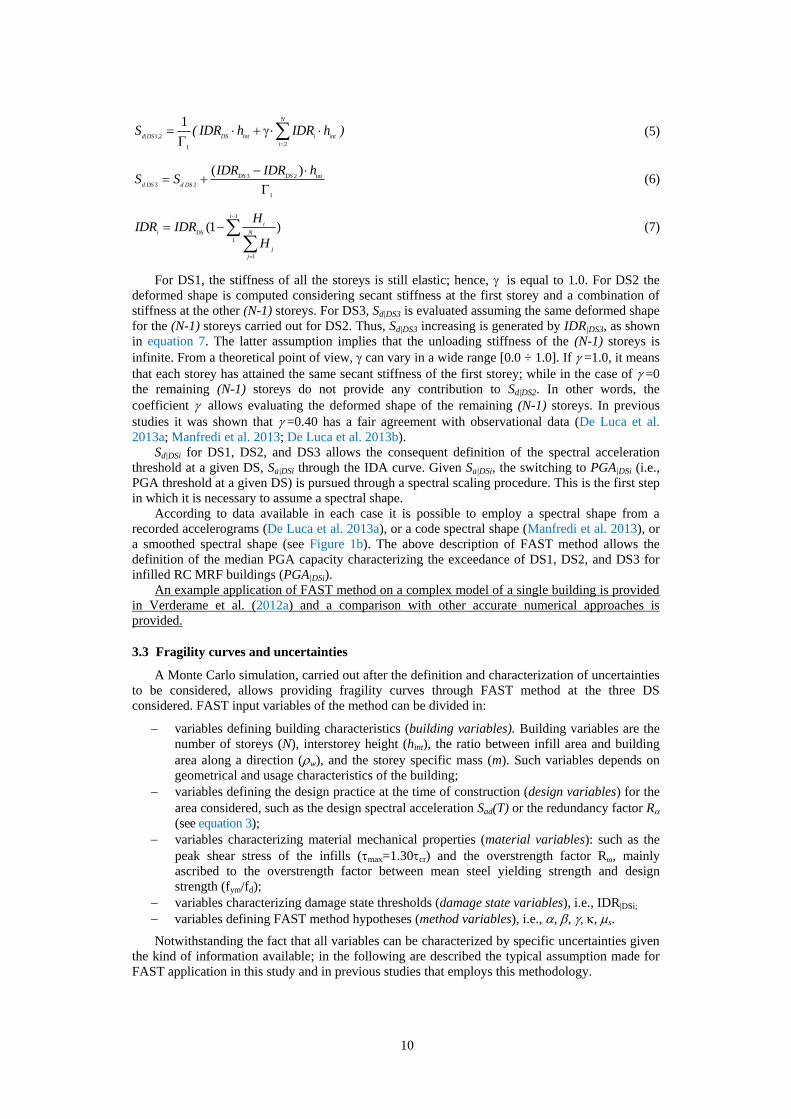
calculated for all the generated samples (see Figure 8), the corresponding cumulative frequency

distributions of the obtained Sa (or PGA) capacities provides the fragility curves at each DS. The

fragility curve at each DS for the single building, independent on the direction, is obtained through

the evaluation of the cumulative frequency distribution of the minimum PGA capacities between

longitudinal and transversal direction (identified by w,x and w,y) for each Monte Carlo sample.

12

Figure 8. Graphical example of generation of fragility curves in FAST method, the black dashed line represent the

estimate through median values of random variables, while grey dashed line represents the jth Monte Carlo sample.

4. FAST CALIBRATION ON PETTINO FRAGILITIES

Observational fragility curves carried out in section 2 allow a calibration of fragilities obtained

via FAST, based on L’Aquila earthquake scenario. The calibration procedure is aimed at defining

key input variables to be assumed in FAST method within ranges that have a counterpart in

experimental and analytical data available in literature. The calibration procedure is carried out in

four basic steps: (i) characterization of input variables from the database; (ii) choice of the

uncertainties to be considered for the evaluation of analytical fragilities; (iii) assumption of the

variables to calibrate, and their numerical ranges; (iv) assumption of an optimizing index to select

the values with the closest agreement between analytical and empirical fragilities.

The first step includes definition of charactering parameters for each building in the database:

N and w are input information provided for each single building (see Figure 3a and 3c). In

particular, the value of w is available for both the directions of the buildings and two capacity

curves are evaluated for each building (one per direction). It is worth noting that for each building

are available dimensions in plan for longitudinal and transversal directions (i.e., Lx, Ly), and w,x

and w,y are computed through the assumption of typical infill thickness. Regarding external infills,

thickness (tw) is considered equal to 20 cm. For the evaluation of internal infills, it is assumed that

their area in each direction is equal to 50% of the area of external infills, in analogy with the

assumption made by Bal et al. (2006). Openings are computed through the strength reduction

coefficients provided by Kakaletsis and Karayannis (2009). In particular, for external infills the

average value of window opening coefficient is assumed (equal to 0.85), while for internal infills

the average value of door opening coefficient is assumed (equal to 0.7). Design is made according

to L’Aquila seismic classification up to 2003 (second category), given age of construction data in

Figure4b, see Ricci et al. (2011a), and Manfredi et al. (2013) for details. R and R are considered

equal to 1.1, and 1.45, respectively, see De Luca et al. (2013a).

The second step of the calibration is the choice of the uncertainties to be considered for the

evaluation of analytical fragilities. Analytical fragilities are the result of four epistemic

uncertainties; in particular cr, and IDR thresholds at each DS considered (IDRDSi). Variability

ascribed to steel yielding strength fy and characterizing R, is not considered, since it is negligible

(≤0.10) with respect to other variables considered in the calibration. For each variable a lognormal

distribution is assumed, and a Monte Carlo simulation is performed for each building of the

database. The fragility curves for the whole database are then collected together to compute

median PGA and standard deviation of logarithms, estimated at each DS. Record to record

variability is not considered since the calibration is provided for the specific scenario of L’Aquila

earthquake. Thus, the approximate IDA for each single building is the median computed through

SPO2IDA. The smooth spectrum in Figure 1b is considered for the switch from Sa to PGA. CoVs

of the random variables considered are not the object of the present calibration. Thus, the whole

process is performed assuming the same CoV for each determination of analytical fragilities at

each DS for the database, and only median values of lognormal distributions vary.

The third step of the calibration process involves the choice of the input variables to be

calibrated. The calibration process will involve median values of the variables characterizing

epistemic uncertainties (cr, IDRDS1, IDRDS2, IDRDS3); Table 3 shows the values assumed for each

13

calibration variable and the assumptions made on the coefficients of variation (CoV) for the

variables. In particular, for cr the CoV value is based on data available in Calvi et al. (2004),

while CoVs for each damage thresholds are those suggested by Colangelo (2012).

The calibration process involves 500 possible combinations of parameters (see the second

column in Table 3) for which the Monte Carlo simulation is performed and results in terms of

fragility curves of the whole database are considered. Medians assumed for the random variables

vary in the ranges provided in section 3.2. Median value of cr is based on experimental, numerical

data (e.g., Colangelo, 2003; Dolsek and Fajfar, 2004), not discarding code suggestions for this

parameter (CS. LL. PP., 2009), covering the range of shear cracking stress for typical Italian

hollow clay brick infills.

Table 3. Simulation values for the calibration of FAST

Calibration Variables Distribution Simulation Values CoV

cr lognormal 0.2 - 0.3 - 0.4 - 0.5 [MPa] 0.30 [Calvi et al. 2004]

IDR|DS1 lognormal 0.2 – 0.4 – 0.6 – 0.8 – 1.0 [‰] 0.67 [Colangelo, 2012]

IDR|DS2 lognormal 2.0 – 2.5 – 3.0 – 3.5 – 4.0 [‰] 0.75 [Colangelo, 2012]

IDR|DS3 lognormal 0.8 – 1.0 – 1.2 – 1.4 – 1.6 [%] 0.50 [Colangelo, 2012]

The fourth step of the calibration is characterized by the choice of a proper optimizing

parameters aimed at compare analytical and observational fragilities. The optimization parameter

selected is the Kullback-Leibler divergence, DKL in the following. In probability theory and

information theory, the DKL is a non-symmetric measure of the difference between two probability

distributions P and Q (Kullback and Leibler, 1951; Kullback, 1959). Specifically, the DKL of Q

from P, denoted DKL(P|Q), is a measure of the information lost when Q is used to approximate P.

Typically, P represents the true distribution of data, observations, or a precisely calculated

theoretical distribution. The measure Q typically represents a theory, model, description, or

approximation of P. If P and Q are continuous random variables and p and q denote the PDF of P

and Q, DKL(P|Q) can be evaluated according to equation 9.

2

( )| log ( )

( )

KL

p xD P Q p x dx

q x (9)

The logarithms in these formulas are taken to base 2, if information is measured in units of

bits; on the other hand, most formulas involving the DKL hold irrespective of log base. DKL(P|Q)

can be seen as the divergence of Q from P as this best relates to the idea that P is considered the

underlying "true" or "best guess" distribution, while Q is some divergent, less good, approximate

distribution. DKL has been used in earthquake engineering as measure of sufficiency of an intensity

measure with respect to another (e.g., Jalayer et al, 2012).

In the context of the calibration provided herein, DKL is seen as the divergence of FAST

analytical fragilities (i.e., Q) with respect to the observational fragilities (i.e., P) provided in

section 2.3 for the three DS considered. Equation 9 is employed considering as p(x), the lognormal

PDF of the observational fragilities, and as q(x) the ith lognormal PDF in terms of PGA, obtained

for the whole population of 131 buildings through Monte Carlo simulations for the ith of the 500

combinations of input variables listed in Table 3. The minimization of DKL evaluated for each DSi

(DKL,DSi) results in one or more than one optimal combinations of cr, and IDR|DSi, that best match

the observational fragilities. It is worth noting that the minimization of DKL,DS1 provides

information on the choice of cr and IDR|DS1, the minimization of DKL,DS2 provides information on

the choice of cr and IDR|DS2, while the minimization of DKL,DS3 provides information on the choice

of cr and IDR|DS3.

The procedure is performed for the three DSs together, so that when evaluating the capacities

in terms of Sd, it is also checked if Sd|DSi is greater or equal with respect to Sd|DSi-1. This kind of

control is made to produce from each simulation a consistent result from FAST at the three DSs,

avoiding that a specific realization provides a Sa and PGA capacity at DSi that is lower with

respect to that evaluated at DSi-1. It is clear that this choice affects also the resulting variability in

the fragility curves at each DS for the single building. Given the ith combination of variables from

the possible 500 combinations considered, the 131 fragilities (one for each building) at each DS

14

are collected together to determine the median PGA and the logarithmic standard deviation of the

lognormal PDF representing the fragility at each DS. Finally, the 500 resulting lognormal PDF

distributions are considered for the evaluation of the DKL,DSi for each of the 500 trials with respect

to the observational fragilities.

4.1 Results

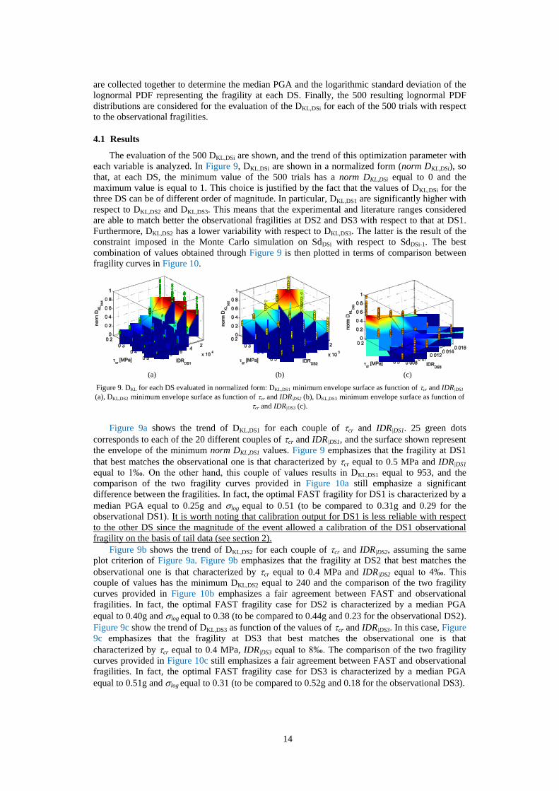
The evaluation of the 500 DKL,DSi are shown, and the trend of this optimization parameter with

each variable is analyzed. In Figure 9, DKL,DSi are shown in a normalized form (norm DKL,DSi), so

that, at each DS, the minimum value of the 500 trials has a norm DKL,DSi equal to 0 and the

maximum value is equal to 1. This choice is justified by the fact that the values of DKL,DSi for the

three DS can be of different order of magnitude. In particular, DKL,DS1 are significantly higher with

respect to DKL,DS2 and DKL,DS3. This means that the experimental and literature ranges considered

are able to match better the observational fragilities at DS2 and DS3 with respect to that at DS1.

Furthermore, DKL,DS2 has a lower variability with respect to DKL,DS3. The latter is the result of the

constraint imposed in the Monte Carlo simulation on SdDSi with respect to SdDSi-1. The best

combination of values obtained through Figure 9 is then plotted in terms of comparison between

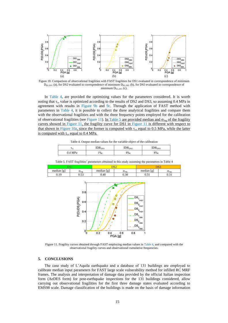
fragility curves in Figure 10.

(a) (b) (c)

Figure 9. DKL for each DS evaluated in normalized form: DKL,DS1 minimum envelope surface as function of cr and IDR|DS1

(a), DKL,DS2 minimum envelope surface as function of cr and IDR|DS2 (b), DKL,DS3 minimum envelope surface as function of

cr and IDR|DS3 (c).

Figure 9a shows the trend of DKL,DS1 for each couple of cr and IDR|DS1. 25 green dots

corresponds to each of the 20 different couples of cr and IDR|DS1, and the surface shown represent

the envelope of the minimum norm DKL,DS1 values. Figure 9 emphasizes that the fragility at DS1

that best matches the observational one is that characterized by cr equal to 0.5 MPa and IDR|DS1

equal to 1‰. On the other hand, this couple of values results in DKL,DS1 equal to 953, and the

comparison of the two fragility curves provided in Figure 10a still emphasize a significant

difference between the fragilities. In fact, the optimal FAST fragility for DS1 is characterized by a

median PGA equal to 0.25g and log equal to 0.51 (to be compared to 0.31g and 0.29 for the

observational DS1). It is worth noting that calibration output for DS1 is less reliable with respect

to the other DS since the magnitude of the event allowed a calibration of the DS1 observational

fragility on the basis of tail data (see section 2).

Figure 9b shows the trend of DKL,DS2 for each couple of cr and IDR|DS2, assuming the same

plot criterion of Figure 9a. Figure 9b emphasizes that the fragility at DS2 that best matches the

observational one is that characterized by cr equal to 0.4 MPa and IDR|DS2 equal to 4‰. This

couple of values has the minimum DKL,DS2 equal to 240 and the comparison of the two fragility

curves provided in Figure 10b emphasizes a fair agreement between FAST and observational

fragilities. In fact, the optimal FAST fragility case for DS2 is characterized by a median PGA

equal to 0.40g and log equal to 0.38 (to be compared to 0.44g and 0.23 for the observational DS2).

Figure 9c show the trend of DKL,DS3 as function of the values of cr and IDR|DS3. In this case, Figure

9c emphasizes that the fragility at DS3 that best matches the observational one is that

characterized by cr equal to 0.4 MPa, IDR|DS3 equal to 8‰. The comparison of the two fragility

curves provided in Figure 10c still emphasizes a fair agreement between FAST and observational

fragilities. In fact, the optimal FAST fragility case for DS3 is characterized by a median PGA

equal to 0.51g and log equal to 0.31 (to be compared to 0.52g and 0.18 for the observational DS3).

15

(a) (b) (c)

Figure 10. Comparison of observational fragilities with FAST fragilities for DS1 evaluated in correspondence of minimum

DKL,DS1 (a), for DS2 evaluated in correspondence of minimum DKL,DS2 (b), for DS3 evaluated in correspondence of

minimum DKL,DS3 (c).

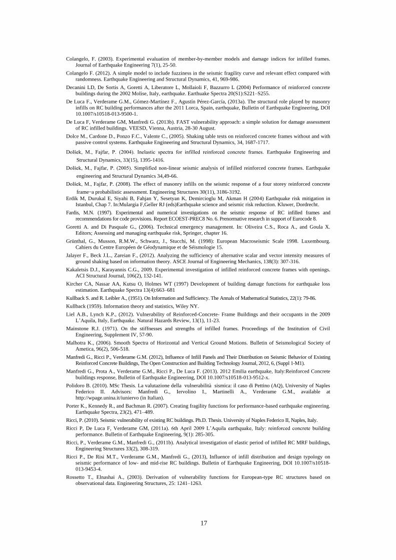
In Table 4, are provided the optimizing values for the parameters considered. It is worth

noting that cr value is optimized according to the results of DS2 and DS3, so assuming 0.4 MPa in

agreement with results in Figure 9b and 9c. Through the application of FAST method with

parameters in Table 4, it is possible to collect the three analytical fragilities and compare them

with the observational fragilities and with the three frequency points employed for the calibration

of observational fragilities (see Figure 11). In Table 5 are provided median and log of the fragility

curves showed in Figure 11, the fragility curve for DS1 in Figure 11 is different with respect to

that shown in Figure 10a, since the former is computed with cr equal to 0.5 MPa, while the latter

is computed with cr equal to 0.4 MPa.

Table 4. Output median values for the variable object of the calibration

cr IDR|DS1 IDR|DS2 IDR|DS3

0.4 MPa 1‰ 4‰ 8‰

Table 5. FAST fragilities’ parameters obtained in this study assuming the parameters in Table 4

DS1 DS2 DS3

median [g] log median [g] log median [g] log

0.19 0.53 0.40 0.38 0.51 0.31

Figure 11. Fragility curves obtained through FAST employing median values in Table 4, and compared with the

observational fragility curves and observational cumulative frequencies.

5. CONCLUSIONS

The case study of L’Aquila earthquake and a database of 131 buildings are employed to

calibrate median input parameters for FAST large scale vulnerability method for infilled RC MRF

frames. The analysis and interpretation of damage data provided by the official Italian inspection

form (AeDES form) for post-earthquake inspections for the 131 buildings considered, allow

carrying out observational fragilities for the first three damage states evaluated according to

EMS98 scale. Damage classification of the buildings is made on the basis of damage information

16

on infill walls from the AeDES form, and though the evaluation of equivalence with EMS98

description of damage to infills for damage states from 1 to 3. The observational fragilities

obtained showed a fair agreement with other fragilities carried out for the same earthquake by

other authors.

Data available for each building of the database allow applying FAST method on the same

database. On the other hand, input data for FAST can vary in quite large intervals according to

experimental and numerical data available in literature. Thus, a calibration procedure on median

variables of the most significant input parameters of the method is carried out. In particular, the

value of the cracking shear stress of the infills, and the interstorey drift (IDR) thresholds, for the

definition of capacity at each damage state, are object of the calibration procedure. The approach

provided allows calibrating median values for each of the four variables considered. Ranges

assumed for each variable considered have always a numerical or experimental counterpart in

literature aimed at obtaining values for each parameter that are compatible with those assumed in

mechanical vulnerability approaches.

Results of calibration emphasize that:

ranges of variables considered allow a fair matching of FAST fragilities with observational

curves for DS2 and DS3 defined according to EMS98;

analytical results are very conservative with respect to observational data for the case of DS1.

FAST method fails to capture the observational fragility at DS1. This result can be justified by

two reasons: (i) the observational classification of DS1 is strictly affected by the operator’s

judgment. DS1 classification often does not have any repair measure as consequence, the building

is very frequently usable, and DS1 mechanical interpretation has weak observational counterpart;

(ii) the database is collected in the epicentral area, characterized by significant values of PGA

registered during the event and the observational DS1 fragility is evaluated on the basis of its right

tail (very high percentiles).

The outcome of the calibration emphasizes the reliability of other FAST applications, since

input variables employed in previous FAST applications, and evaluated on mechanical basis, are

quite similar with the results obtained in this calibration study. Finally, it can be emphasized that

FAST method can be a useful and straightforward method for large scale post-emergency

vulnerability analyses aimed at the prioritization of interventions.

ACKNOWLEDGEMENTS

The work presented has been developed in cooperation with Rete dei Laboratori Universitari di Ingegneria

Sismica—ReLUIS—Linea 1.1.2. for the research program funded by the Dipartimento della Protezione Civile

(2010–2013). The authors would like also to thank Eng. Raffaele Incarnato for his help with GIS data and his

cooperation for the evaluation of observational fragilities, and Dr. Barbara Polidoro for her help with the data

from her M.Sc thesis.

REFERENCES

American Society of Civil Engineers, ASCE, (2007). Seismic Rehabilitation of Existing Buildings, ASCE/SEI 41-06,

Reston, Virginia.

Bal I, Crowley H, Pinho R, Gulay G. (2006). Structural Characterisation of Turkish R/C Building Stock for Loss

Assessment Applications, Proceedings of 1st European Conference of Earthquake Engineering and Seismology,

Geneva, paper n° 603.

Baggio C., Bernardini A., Colozza R., Della Bella M., Di pasquale G., Dolce M., Goretti A., Martinelli A., Orsini G., Papa

F., and Zuccaro G., (2000). Field manual for the I level post-earthquake damage, usability and emergency measures

from. National Seismic Survey and National Group for Defence against Earthquakes.

Calvi GM, Bolognini D, Penna A (2004) Seismic Performance of masonry-infilled RC frames–benefits of slight

reinforcements. Invited lecture to “Sísmica 2004—6◦ Congresso Nacional de Sismologia e Engenharia Sísmica”,

Guimarães, Portugal, April 14–16.

Chioccarelli E, De Luca F, Iervolino I (2009) Preliminary study on L’Aquila earthquake ground motion records, V5.20.

http://www.reluis.it/

CEN, (2004). European Standard EN1998-1:2004. Eurocode 8: Design of structures for earthquake resistance. Part 1:

general rules, seismic actions and rules for buildings. Comité Européen de Normalisation, Brussels.

Circolare del Ministero dei Lavori Pubblici n. 617 del 2/2/2009 (2009) Istruzioni per l’applicazione delle “Nuove norme

tecniche per le costruzioni” di cui al D.M. 14 gennaio 2008. G.U. n. 47 del 26/2/2009 (in Italian).

17

Colangelo, F. (2003). Experimental evaluation of member-by-member models and damage indices for infilled frames.

Journal of Earthquake Engineering 7(1), 25-50.

Colangelo F. (2012). A simple model to include fuzziness in the seismic fragility curve and relevant effect compared with

randomness. Earthquake Engineering and Structural Dynamics, 41, 969-986.

Decanini LD, De Sortis A, Goretti A, Liberatore L, Mollaioli F, Bazzurro L (2004) Performance of reinforced concrete

buildings during the 2002 Molise, Italy, earthquake. Earthuake Spectra 20(S1):S221–S255.

De Luca F., Verderame G.M., Gómez-Martínez F., Agustín Pérez-García, (2013a). The structural role played by masonry

infills on RC building performances after the 2011 Lorca, Spain, earthquake, Bulletin of Earthquake Engineering, DOI

10.1007/s10518-013-9500-1.

De Luca F, Verderame GM, Manfredi G. (2013b). FAST vulnerability approach: a simple solution for damage assessment

of RC infilled buildings. VEESD, Vienna, Austria, 28-30 August.

Dolce M., Cardone D., Ponzo F.C., Valente C., (2005). Shaking table tests on reinforced concrete frames without and with

passive control systems. Earthquake Engineering and Structural Dynamics, 34, 1687-1717.

Dolšek, M., Fajfar, P. (2004). Inelastic spectra for infilled reinforced concrete frames. Earthquake Engineering and

Structural Dynamics, 33(15), 1395-1416.

Dolšek, M., Fajfar, P. (2005). Simplified non-linear seismic analysis of infilled reinforced concrete frames. Earthquake

engineering and Structural Dynamics 34,49-66.

Dolšek, M., Fajfar, P. (2008). The effect of masonry infills on the seismic response of a four storey reinforced concrete

frame—a probabilistic assessment. Engineering Structures 30(11), 3186-3192.

Erdik M, Durukal E, Siyahi B, Fahjan Y, Sesetyan K, Demircioglu M, Akman H (2004) Earthquake risk mitigation in

Istanbul, Chap 7. In:Mulargia F,Geller RJ (eds)Earthquake science and seismic risk reduction. Kluwer, Dordrecht.

Fardis, M.N. (1997). Experimental and numerical investigations on the seismic response of RC infilled frames and

recommendations for code provisions. Report ECOEST-PREC8 No. 6. Prenormative research in support of Eurocode 8.

Goretti A. and Di Pasquale G., (2006). Technical emergency management. In: Oliveira C.S., Roca A., and Goula X.

Editors; Assessing and managing earthquake risk, Springer, chapter 16.

Grünthal, G., Musson, R.M.W., Schwarz, J., Stucchi, M. (1998): European Macroseismic Scale 1998. Luxembourg.

Cahiers du Centre Européen de Géodynamique et de Séismologie 15.

Jalayer F., Beck J.L., Zareian F., (2012). Analyzing the sufficiency of alternative scalar and vector intensity measures of

ground shaking based on information theory. ASCE Journal of Engineering Mechanics, 138(3): 307-316.

Kakaletsis D.J., Karayannis C.G., 2009. Experimental investigation of infilled reinforced concrete frames with openings.

ACI Structural Journal, 106(2), 132-141.

Kircher CA, Nassar AA, Kutsu O, Holmes WT (1997) Development of building damage functions for earthquake loss

estimation. Earthquake Spectra 13(4):663–681

Kullback S. and R. Leibler A., (1951). On Information and Sufficiency. The Annals of Mathematical Statistics, 22(1): 79-86.

Kullback (1959). Information theory and statistics, Wiley NY.

Liel A.B., Lynch K.P., (2012). Vulnerability of Reinforced-Concrete- Frame Buildings and their occupants in the 2009

L’Aquila, Italy, Earthquake. Natural Hazards Review, 13(1), 11-23.

Mainstone R.J. (1971). On the stiffnesses and strengths of infilled frames. Proceedings of the Institution of Civil

Engineering, Supplement IV, 57-90.

Malhotra K., (2006). Smooth Spectra of Horizontal and Vertical Ground Motions. Bulletin of Seismological Society of

Ametica, 96(2), 506-518.

Manfredi G., Ricci P., Verderame G.M. (2012), Influence of Infill Panels and Their Distribution on Seismic Behavior of Existing

Reinforced Concrete Buildings, The Open Construction and Building Technology Journal, 2012, 6, (Suppl 1-M1).

Manfredi G., Prota A., Verderame G.M., Ricci P., De Luca F. (2013). 2012 Emilia earthquake, Italy:Reinforced Concrete

buildings response, Bulletin of Earthquake Engineering, DOI 10.1007/s10518-013-9512-x.

Polidoro B. (2010). MSc Thesis. La valutazione della vulnerabilità sismica: il caso di Pettino (AQ), University of Naples

Federico II. Advisors: Manfredi G., Iervolino I., Martinelli A., Verderame G.M., available at

http://wpage.unina.it/iuniervo (in Italian).

Porter K., Kennedy R., and Bachman R. (2007). Creating fragility functions for performance-based earthquake engineering.

Earthquake Spectra, 23(2), 471–489.

Ricci, P. (2010). Seismic vulnerability of existing RC buildings. Ph.D. Thesis. University of Naples Federico II, Naples, Italy.

Ricci P, De Luca F, Verderame GM, (2011a). 6th April 2009 L’Aquila earthquake, Italy: reinforced concrete building

performance. Bulletin of Earthquake Engineering, 9(1): 285-305.

Ricci, P., Verderame G.M., Manfredi G., (2011b). Analytical investigation of elastic period of infilled RC MRF buildings,

Engineering Structures 33(2), 308-319.

Ricci P., De Risi M.T., Verderame G.M., Manfredi G., (2013), Influence of infill distribution and design typology on

seismic performance of low- and mid-rise RC buildings. Bulletin of Earthquake Engineering, DOI 10.1007/s10518-

013-9453-4.

Rossetto T., Elnashai A., (2003). Derivation of vulnerability functions for European-type RC structures based on

observational data. Engineering Structures, 25: 1241–1263.

18

Sezen H., Whittaker A.S., Elwood K.J., Mosalam K.M., (2003). Performance of reinforced concrete buildings during the

August 17, 1999 Kocaeli, Turkey earthquake, and seismic design and construction practise in Turkey. Engineering

Structures, 25(1):103-114.

Tothong P., Cornell C.A., (2007). Probabilistic seismic demand analysis using advanced ground motion intensity measures,

attenuation relationships, and near fault effects. John A. Blume Earthquake Engineering Center, Department of Civil

and Environmental Engineering, Stanford University, CA 2007.

Vamvatsikos D. and Cornell C.A., (2006). Direct estimation of the seismic demand and capacity of oscillators with multi-

linear static pushovers through Incremental Dynamic Analysis. Earthquake Engineering and Structural Dynamics,

35(9), 1097-1117.

Vamvatsikos D, Fragiadakis M. (2010). Incremental dynamic analysis for estimating seismic performance sensitivity and

uncertainty. Earthquake Engineering and Structural Dynamics, 39: 141-163.

Verderame GM, Polese M, Mariniello C, Manfredi G (2010) A simulated design procedure for the assessment of seismic

capacity of existing reinforced concrete buildings. Advances in Engineering Software 41:323–335.

Verderame GM, De Luca F, Ricci P, Manfredi G. (2011) Preliminary analysis of a soft-storey mechanism after the

2009L’Aquila earthquake. Earthquake Engineering and Structural Dynamics, 40(8): 925-944.

Verderame G.M., De Luca F., De Risi M.T., Del Gaudio C., Ricci P., (2012a). A three level vulnerability approach for

damage assessment of infilled RC buildings: The Emilia 2012 case (V 1.0), available at http://www.reluis.it/.

Verderame GM, Ricci P, Esposito M, Manfredi G (2012b) STIL v1.0–Software per la caratterizzazione delle proprietà

meccaniche degli acciai da c.a. tra il 1950 e il 2000, available at http://www.reluis.it/

Walters R.J., Elliott J.R., D’Agostino N., England P.C., Hunstad I., Jackson J.A., Parsons B., Philips R.J., and Roberts G.,

(2009). The 2009 L’Aquila earthquake (central Italy): a source mechanism and implications for seismic hazard.

Geophysical Research Letters, 36, L17312.