Day-Ahead and Real-Time Modelsfor Large-Scale Energy Storage

Final Project Report

Power Systems Engineering Research Center

Empowering Minds to Engineerthe Future Electric Energy System

Day-Ahead and Real-Time Models for Large-Scale Energy Storage

Final Project Report

Project Team

Kory W. Hedman, Project Leader Arizona State University

Ward Jewell Wichita State University

Graduate Students:

Nan Li Arizona State University

Haneen Aburub Wichita State University

PSERC Publication 15-02

September 2015

For information about this project, contact Kory W. Hedman Arizona State University School of Electrical, Computer, and Energy Engineering P.O. BOX 875706 Tempe, AZ 85287-5706 Phone: 480 965-1276 Fax: 480 965-0745 Email: kory.hedman@asu.edu Power Systems Engineering Research Center The Power Systems Engineering Research Center (PSERC) is a multi-university Center conducting research on challenges facing the electric power industry and educating the next generation of power engineers. More information about PSERC can be found at the Center’s website: http://www.pserc.org. For additional information, contact: Power Systems Engineering Research Center Arizona State University 527 Engineering Research Center Tempe, Arizona 85287-5706 Phone: 480-965-1643 Fax: 480-965-0745 Notice Concerning Copyright Material PSERC members are given permission to copy without fee all or part of this publication for internal use if appropriate attribution is given to this document as the source material. This report is available for downloading from the PSERC website.

2015 Arizona State University. All rights reserved.

i

Acknowledgements

This is the final report for the Power Systems Engineering Research Center (PSERC) research project titled “Day-ahead and real-time models for large-scale energy storage” (project S-61G). We express our appreciation for the support provided by PSERC’s industry members and by the National Renewable Energy Laboratory under the Industry / University Cooperative Research Center program. This work was supported by the U.S. Department of Energy under Contract No. DE-AC36-08GO28308 with the National Renewable Energy Laboratory. Funding provided by the U.S. DOE Office of Energy Efficiency and Renewable Energy Wind and Water Power Technologies Office.

The authors also thank the industry advisors for this project: Aftab Alam (CAISO), Rudy Bombien (DUKE), Hong Chen (PJM), Charlton Clark (DOE), Vikas X. Dawar (NYISO), Paul Denholm (NREL), Erik Ela (EPRI), Bruce Fardanesh (NYPA), Xiaoming Feng (ABB), Eduardo Ibanez (NREL), Nikhil Kumar (GE), Deepak Maragal, (NYPA), Khosrow Moslehi (ABB), Nivad Navid (MISO), Hussam Sehwail (ITC Holdings), Alva Svoboda (PG&E), Xing Wang (Alstom Grid), Sean Wright (EPRI), Zheng Zhou (MISO).

ii

Executive Summary

With the stringent fleet challenges introduced by renewable resources, the need for flexible resources in power systems is higher than ever. Since energy storage has energy shifting and fast-ramping capabilities, it provides an attractive solution to facilitate the integration of high levels of renewable resources. While there are growing interests in energy storage in recent years, the existing market structure does not always account for the characteristics of energy storage. As a result, the full flexibility of energy storage is not being used by the existing energy management systems and market management systems. In this report, the primary goal is to develop commitment and dispatch optimization models that optimally utilize large-scale storage at multiple time scales and horizons as well as to have scalable formulations and algorithms. Due to its significance as the most common form of large-scale energy storage, the work is focused on pumped hydro storage (PHS). The report is presented in two parts.

Part I: A Study of Adjustable-Speed Pumped Storage Hydro Operation in the US Day-ahead Market

The 40 open-loop fixed-speed PHS facilities operating in the U.S. total more than 20 GW of storage capacity, approximately 2% of U.S. generating capacity. In today’s market regions, the generation and pumping of PHS follow consistent daily patterns, pumping at night and generating on peak. With increasing levels of new technologies, like wind, solar, and distributed generation,, it may be that these are not always the periods of time that require these modes of operation. However, advanced optimization of commitment and dispatch schedules is needed in order to determine the optimal operation of these plants. In addition, PHS plants that utilize adjustable speed (AS) pumping technology will provide further flexibility. Full optimization of PHS and other energy storage is computationally difficult and requires additional data, and AS capability adds additional complexity to the optimization.

Part I presents a day-ahead unit commitment and economic dispatch model that allows for the optimization of AS PHS. The model is implemented in open-source optimal power flow software. It is then demonstrated on a reduced 240-bus model of the WECC system to study the future operation of AS technology under two variable renewable penetrations, 6% and 14%, and two different optimization scenarios. The cycling costs for conventional generation are included in the models.

The results show that AS PHS provides benefits in all cases. Energy arbitrage alone, however, may not provide the needed financial incentives for AS PHS, especially when high renewable penetrations are present in the system. Ancillary services markets may provide the additional needed incentives. When the cycling costs of conventional generators are considered, even more cost savings can be obtained by optimizing PHS operations.

Increasing the penetration level of renewables significantly increased the complexity in the system, and this was shown in higher solution times. Optimizing PHS while

iii

considering the cycling cost reduces the total system operating cost and improves the DA market operation. Full optimization of AS PHS while considering the cycling cost resulted in the best total system cost savings, solving time, and PHS revenues. More AS PHS needs to be present in the system as renewable penetrations increase to provide fast ramping to follow renewable variations and thus reduce the cycling of coal and gas generators.

Part II: Enhanced Pumped Hydro Storage Model in Real-Time Operations This part of the report investigates the modeling of different PHS technologies and develops an improved approach to enhance the utilization of the PHS in real-time operation.

Two types of PHS technologies are studied in the report, namely the traditional fixed-speed PHS and the adjustable-speed PHS. For the fixed-speed PHS, the pumping power is fixed and cannot be varied in the pumping mode. Therefore, the fixed-speed PHS can only provide regulation reserves in the generation mode. However, for the adjustable-speed PHS, the power is adjustable in the pumping mode. With this improvement, the adjustable-speed PHS is able to provide regulation and load following reserves in both the pumping and generation mode. It also has higher round-trip efficiencies compared to the fixed-speed PHS. A two-step approach is proposed to evaluate and compare the attractiveness of the fixed-speed and the adjustable-speed PHS in integrating variable renewable generation. The two-step approach simulates the scheduling and the deployment of regulation reserves via AGC. The result shows that the adjustable-speed PHS is able to provide large quantities of regulation reserves in both the generation and the pumping mode. By having the capability to provide regulation reserves in both the generation and pumping mode, the adjustable-speed is a more effective solution to manage the uncertainty and variability introduced by renewable resources.

While energy storage has been considered as an attractive resource to meet the increasing need for flexible resources, existing market structure does not adequately account for the characteristics of energy storage. Today, the existing real-time market has a limited look-ahead time window and do not look hours in advance. As the value of energy storage is dependent on the future value of the resource at a later time stage, the flexibility of energy storage is not being fully utilized by the existing market structure. To enhance the utilization of the PHS in real-time operation, a policy function based approach is proposed in the report. A policy function is a rule that describes the control action as a function of the state. In the report, the policy function is generated using random forest classification algorithms. Given an operating state, the policy function can return a dispatch decision for the PHS taking into account both the current and future operating conditions. By shifting computational complexity to offline analysis, the policy function based approach has minimal added computational difficulty to the existing energy management systems in real-time. In the case study, the result shows that the policy function based approach has better performance compared to the existing approach, where the PHS is operated based schedules that are determined through a prior look-ahead planning stage. The result in the case study also indicates that the policy function based approach has close performance to the stochastic programming model based

iv

benchmark and the perfect-foresight benchmark. By using the proposed approach, the utilization of the PHS is enhanced with minimal added computational difficulty to the existing energy management systems and market management systems.

In summary, the key takeaway points of this project are,

• The fixed-speed PHS and the adjustable-speed PHS are investigated in the report. With increasing renewable penetrations, the case study shows that the adjustable-speed PHS is a more attractive and effective solution to balance the uncertainties introduced by renewable resources.

• In this report, a policy function based approach is proposed to enhance the utilization of the PHS in systems with renewable resources.

• The policy function is generated using a data mining approach, referred to as a classification technique.

• In real-time operations, the policy function can return a decision for the PHS given the system operational conditions, while also taking into account future uncertainties in the system.

• The result shows that the proposed policy function based approach has performance close to a stochastic programming model based benchmark while having minimal added computational difficulty to the existing energy management systems and market management systems.

• While a classification technique is used to generate the policy function in this report, the policy function can also be derived using other techniques or be designed in other forms. The policy function based approach has tractable computational complexity for a large-scale power system and can also effectively enhance the utilization of PHS. The policy function based approach is a scalable approach that can be applied to a “real-world” power system and energy market.

Project Publications: N. Li, C. Uckun, E. Constantinescu, J. R. Birge, K. W. Hedman, and A. Botterud, “Flexible operation of batteries in power system with renewable energy,” IEEE Transactions on Sustainable Energy, under review. N. Li, and K. W. Hedman, “Enhanced utilization of pumped hydro storage in power system operation using policy functions,” IEEE Transactions on Power System, in preparation. N. Li, M. Hedayati and K. W. Hedman, “Using flywheels to provide regulation services for systems with renewable resources,” 2015 IEEE Power and Energy Society General Meeting, accepted.

v

H. Aburub and W. Jewell, "Optimal Generation Planning to Improve Storage Cost and System Conditions," IEEE Power and Energy Society General Meeting, Washington, July 2014.

H. Aburub and W. Jewell, “A Study of Adjustable-Speed Pumped Storage Hydro Operation in the US Day-ahead Market,” to be submitted to IEEE Transactions on Sustainability.

Student Theses: Nan Li. Let Wind Rise – Harnessing Bulk Energy Storage under High Renewable Penetration Levels. PhD dissertation, Arizona State University, Tempe AZ, expected in January 2016. Haneen Aburub, Electric Energy Storage for High Penetration Renewables, PhD Dissertation, Wichita State University, Wichita, Kansas, USA, expected May 2016.

Part I

A Study of Adjustable-Speed Pumped Hydro Storage Operation in the US Day-ahead Market

Haneen Aburub Ward Jewell

Wichita State University

For information about this project, contact Ward Jewell Wichita State University Department of Electrical Engineering and Computer Science Wichita, Kansas, USA 67260-0083 Phone: 316-978-6340 Email: ward.jewell@wichita.edu Power Systems Engineering Research Center The Power Systems Engineering Research Center (PSERC) is a multi-university Center conducting research on challenges facing the electric power industry and educating the next generation of power engineers. More information about PSERC can be found at the Center’s website: http://www.pserc.org. For additional information, contact: Power Systems Engineering Research Center Arizona State University 527 Engineering Research Center Tempe, Arizona 85287-5706 Phone: 480-965-1643 Fax: 480-965-0745 Notice Concerning Copyright Material PSERC members are given permission to copy without fee all or part of this publication for internal use if appropriate attribution is given to this document as the source material. This report is available for downloading from the PSERC website.

2015 Wichita State University. All rights reserved.

i

Table of Contents

Table of Contents ................................................................................................................. i

List of Figures ..................................................................................................................... ii

List of Tables ..................................................................................................................... iii

Nomenclature ..................................................................................................................... iv

1. Introduction ................................................................................................................... 1

1.1 Background ........................................................................................................... 1

1.2 Summary of Chapters ........................................................................................... 2

2. Problem Formulation: Optimization Model.................................................................. 3

3. WECC System Data and Assumptions ......................................................................... 6

3.1 Simulation Time Period ........................................................................................ 6

3.2 WECC PHS Plants ............................................................................................... 6

3.3 WECC Conventional Generators ......................................................................... 7

3.4 Generator Cycling Costs ....................................................................................... 8

3.5 WECC Renewables .............................................................................................. 9

4. Results ......................................................................................................................... 11

4.1 Conventional Generator Cycling Costs Included ............................................... 11

4.2 Conventional Generator Cycling Costs Not Included ........................................ 12

4.3 Effects of Including Conventional Generator Cycling Costs ............................. 13

4.4 Solution Time and PHS Revenues ..................................................................... 14

4.5 Conventional Generator Cycling ........................................................................ 16

5. Conclusions ................................................................................................................. 18

6. Future Work ................................................................................................................ 19

References ......................................................................................................................... 20

ii

List of Figures

Fig. 3.1. WECC model generation mix [8] ......................................................................... 6

Fig. 3.2. Renewables and load generation within the 672-hour simulation horizon. ....... 10

Fig. 4.1. Coal and gas generation for fully-optimized PHS and cycling cost considered under low and high renewables penetration level. ............................................................ 16

Fig. 4.2. Coal and gas generation for no PHS and cycling cost considered under low and high renewables penetration level ..................................................................................... 17

iii

List of Tables

Table 3.1. WECC PHS Plant Specifications ....................................................................... 7

Table 3.2. WECC Conventional Generator Costs .............................................................. 8

Table 3.3. WECC Generator Variable Costs ...................................................................... 9

Table 4.1. High Renewable with Cycling Cost Relative to No PHS Model Case ............ 11

Table 4.2. Low Renewable with Cycling Cost Relative to No PHS Model Case ............ 12

Table 4.3. High Renewable with No Cycling Cost Relative to No PHS Model Case ...... 13

Table 4.4. Low Renewable with No Cycling Cost Relative to No PHS Model Case ...... 13

Table 4.5. High Renewable, effects of considering cycling costs .................................... 14

Table 4.6. Low Renewable, effects of considering cycling costs ..................................... 14

Table 4.7. Solving Time and PHS Revenues .................................................................... 15

iv

Nomenclature

𝐵𝑓 Analogous to the system Y matrix

𝐶𝑐𝑖 Cycling cost function of generator i

𝐶𝐶 Capacity factor of generator i

𝐶𝑔𝑖 Cost function of generator i

𝐶𝑆𝑆𝑖 Start-up cost function of generator i

𝐸𝑠𝑖𝑖 Energy status of PHS plant at time t

𝐸𝑠𝑠𝑠𝑠𝑖 Maximum energy capacity of PHS plant at time t

𝐸𝑠𝑠𝑖𝑠𝑖 Minimum energy capacity of PHS plant at time t

𝐶𝑠𝑠𝑠 Vector of branch flow limit

𝐺𝑠ℎ Vector of approximated active power consumed by shunt elements

𝑃𝑑𝑏 Active power demand at bus b

𝑃𝑔𝑏 Active power generation at bus b

𝑃𝑠ℎ𝑖𝑓𝑖𝑏 Active power shift at bus b

𝑃𝑔𝑖𝑖 Active power output of generator i at time t

𝑃𝑔𝑐𝑖𝑖 Consumed active power of virtual PHS dispatchable load at time t

𝑃𝑔𝑑𝑖𝑖 Produced active power of virtual PHS generator i at time t

𝑃𝑠𝑠𝑠𝑖 Maximum active power output of generator i

𝑃𝑠𝑖𝑠𝑖 Minimum active power output of generator i

𝑃𝑟𝑖 Active power ramping limit of PHS plant i

𝑃𝑠𝑖𝑖 Active power output of PHS plant i at time t

𝑃𝑠𝑠𝑠𝑠𝑖 Maximum active power output of PHS plant i at time t

𝑃𝑠𝑠𝑖𝑠𝑖 Minimum active power output of PHS plant i at time t

𝑢𝑔𝑖𝑖 Commitment status of generator i at time t

v

𝑣𝑔𝑆𝑔𝑖𝑖 Shut-down status of generator i at time t

𝑣𝑔𝑆𝑆𝑖𝑖 Start-up status of generator i at time t

𝜃𝑖 Angle at bus i

𝜃𝑠𝑠𝑠𝑖 Maximum angle at bus i

𝜃𝑠𝑖𝑠𝑖 Minimum angle at bus i

𝜂𝑑𝑖 Discharging efficiency of PHS plant i

𝜂𝑐𝑖 Charging efficiency of PHS plant i

1

1. Introduction

1.1 Background

Energy storage technologies play an increasingly important role in improving the reliability and reducing the production cost of the electric power system by providing energy and ancillary services to the grid. The most common utility-sized energy storage technology is the pumped hydro storage (PHS) [1]. Currently, there are 40 open-loop (using a naturally-flowing stream or reservoir) fixed-speed (FS) PHS plants operating in the U.S. totaling more than 20 GW of storage capacity (approximately 2% of U.S. generating capacity) [2]. In 1929, the Rocky River facility was the first PHS plant constructed in North America on the Housatonic River in Connecticut with a capacity of 31 MW [3]. During the mid- to late 1970s, the significant increase in oil and gas prices and concerns about the security of fuel supplies resulted in building the majority of PHS capacity [1]. Recently, the Federal Energy Regulatory Commission (FERC) had granted preliminary permits for 50 PHS projects with a total of 34 GW capacity over 22 states, which would more than double the existing capacity [2,3]. Many of these projects are for closed-loop sites, and are considering the use of adjustable speed (AS) technology [3,4]. A preliminary permit does not authorize construction; however it strongly indicates the interest in PHS development [4]. The flexibility of PHS, especially with its AS technology, will play an important role in integrating high penetration level of variable renewables due to its fast ramping capability, low operating cost, and the ability of AS technology to vary the power consumed in the pumping and generating modes over a range of values [3,5]. In the U.S. deregulated markets, except for PJM, the PHS operation is sub-optimized by the independent system operators (ISOs) [3]. ISOs require that PHS choose the generation and pumping mode periods in advance of the day-ahead (DA) market, and then the ISO decides the commitment status, energy and ancillary services schedules of the plant in that operation mode. Unlike other ISOs, PJM fully optimizes the PHS in its DA market by also deciding generation and pumping periods [3].

Full optimization of PHS is computationally very difficult and requires additional data sets. This could be seen when the solution time of PJM’s system optimizer was increased 5 to 10 times by the addition of a single PHS plant [3]. In today’s market regions the PHS generation and pumping follow consistent daily patterns (e.g. pumping at night and generation in peak load periods). The unique characteristics of PHS with full optimization will be more needed when there are higher penetrations of variable generation because at that time, the marginal prices have much more volatility throughout the day [3]. Since currently there are no AS PHS plants in the U.S., the work proposed in this paper developed an open-loop AS PHS DA unit commitment and economic dispatch optimization model, which is demonstrated on a reduced 240-bus WECC system to study the future operation of AS technology under different penetration levels of renewables and different optimization scenarios.

2

1.2 Summary of Chapters

This report is structured as follows. In chapter 2, the optimization models are developed. There is one model for full optimization, and another one for a suboptimal solution. Both include AS operation of PHS in both generation and pumping modes.

Chapter 3 presents the data and assumptions used to model the WECC system. New information, including cycling costs for conventional generators, was needed for this research, and is presented in chapter 3.

Chapter 4 presents the results of running the optimization models on the WECC system. Chapter 5 is the conclusions drawn from the work, and chapter 6 presents ideas for continuing work on this subject.

3

2. Problem Formulation: Optimization Model

In this chapter, the optimization model is presented in equations (1) through (24). This model was built in the MATPOWER environment [7] using its standard and extensible optimal power flow (OPF) structure. MATPOWER is a package of MATLAB M-files for solving power flow and optimal power flow problems [7]. For simplicity, DC OPF formulations were used in the model because of its faster solution time. Many industrial and commercial OPF formulations use the DC equations to get satisfactory results [6]. The techniques developed will also apply to ac OPF, but the use of ac OPF in this paper would increase the complexity and solutions times to impractical levels.

The optimization model is formed as a quadratic programming problem that approximate the DA unit commitment (UC) and economic dispatch (ED) market behavior. Quadratic programming is used because MATPOWER does not support defining binary variables that reflect the commitment, start-up, and shut-down status. Quadratic programming is a special form of nonlinear programming in which the objective function is quadratic and all constraints are linear [6].

The objective function developed specifically for this work is shown in equation (1). It includes the conventional quadratic and linear generation cost function 𝐶𝑔, and linear start-up cost function 𝐶𝑆𝑆. It adds to these a linear cycling cost function 𝐶𝑐, which is needed because generators are cycling more to follow variable generation as penetrations of variable generation increase. This is an important contribution of this work and it is discussed in more detail in part B of this section.

Equations (2) through (6) represent the standard DC OPF variables and constraints applied in MATPOWER and other DC OPF models such as [12]. This formulation includes angle 𝜃, active power 𝑃𝑔, branch, and bus power limits [7]. Hydro optimization is presented by equation (7). In Equation (7), all hydro units are assumed to have the same capacity factor (CF) value during the simulation horizon.

The next important contribution of this work is equations (8) through (17), which represent the AS PHS optimization model. In this model, the storage is modeled as dispatchable load 𝑃𝑔𝑐 and generation 𝑃𝑔𝑑, in which the summation of their outputs results in the storage output. Equations (16) and (17) show the full and sub-optimization cases of AS PHS respectively. In equation (16) the PHS can flexibly change its pumping output between the minimum and maximum capacity of the virtual dispatchable load that represents the pumping mode of PHS. In addition, equation (16) allows the full optimization by committing and dispatching the pumping and generating schedules. Unlike equation (16), in equation (17) the pumping and generating times are provided by the PHS owner, which results in a sub-optimal solution.

The UC optimization model is represented by equations (19) through (24). The MATPOWER capability to run an OPF combined with a unit de-commitment for a single time period was applied in this paper. This capability allows it to shut down the most expensive units and thus find the least cost commitment and dispatch [7]. This work

4

extends the work developed in [9] and [13] by adding a detailed ramping model in equation (15) for AS PHS, and its optimization options in equations (16) and (17). The generation UC commitment and cycling operation of conventional generators are important additions to the previous work done in [9] and [13]. These are used to study the benefits of AS PHS in the future variable DA market in the US.

𝑚𝑚𝑚𝜃,𝑃𝑔,𝑃𝑠,𝐸𝑠,𝑢,𝑣𝑆𝑆,𝑣𝑆𝑆 ∑ 𝐶𝑔𝑖(𝑃𝑔𝑖𝑖)𝑖 + ∑ 𝐶𝑐𝑖(𝑖 𝑃𝑔𝑖𝑖 − 𝑃𝑔𝑖(𝑖+1)) + ∑ 𝐶𝑆𝑆𝑖 (𝑣𝑆𝑆𝑖𝑖 )𝑖 (1)

𝜃𝑠𝑖𝑠𝑖 ≤ 𝜃𝑖 ≤ 𝜃𝑠𝑠𝑠𝑖 (2)

𝑃𝑠𝑖𝑠𝑖 ≤ 𝑃𝑔𝑖𝑖 ≤ 𝑃𝑠𝑠𝑠𝑖 (3)

𝐵𝑓𝜃 + 𝑃𝑓,𝑠ℎ𝑖𝑓𝑖 − 𝐶𝑠𝑠𝑠 ≤ 0 (4)

−𝐵𝑓𝜃 − 𝑃𝑓,𝑠ℎ𝑖𝑓𝑖 − 𝐶𝑠𝑠𝑠 ≤ 0 (5)

𝐵𝑏𝜃 + 𝑃𝑠ℎ𝑖𝑓𝑖𝑏 + 𝑃𝑑𝑏 + 𝐺𝑠ℎ − 𝑃𝑔𝑏 ≤ 0 (6)

∑ 𝑃𝑔𝑖 ≤ 𝐶𝐶 ∑ 𝑃max𝑖𝑖𝑖 (7)

−𝑃𝑠𝑠𝑠𝑠𝑖 ≤ 𝑃𝑠𝑖𝑖 ≤ 𝑃𝑠𝑠𝑠𝑠𝑖 (8)

−𝐸𝑠𝑠𝑠𝑠𝑖 ≤ 𝐸𝑠𝑖𝑖 ≤ 𝐸𝑠𝑠𝑠𝑠𝑖 (9)

0 ≤ 𝑃𝑔𝑐𝑖𝑖 ≤𝐸𝑠𝑠𝑠𝑠𝑖 −𝐸𝑠

𝑖(𝑡−1)

𝜂𝑐𝑖 (10)

0 ≤ 𝑃𝑔𝑑𝑖𝑖 ≤ 𝐸𝑠𝑖(𝑖−1)𝜂𝑑𝑖 (11)

0 ≤ ∑ 𝑃𝑔𝑐𝑖𝑖 ≤ 𝐸𝑠𝑠𝑠𝑠𝑖 −𝐸𝑠

𝑖(𝑡−1)

𝜂𝑐𝑖−

𝑃𝑔𝑔𝑖(𝑡−1)

𝜂𝑐𝑖𝜂𝑔𝑖 (12)

0 ≤ ∑ 𝑃𝑔𝑑𝑖𝑖 ≤ 𝐸𝑠𝑖(𝑖−1)𝜂𝑑𝑖 − 𝜂𝑐𝑖 𝜂𝑑𝑖 𝑃𝑔𝑐

𝑖(𝑖−1) (13)

∑ 𝑃𝑔𝑐𝑖𝑖 + ∑ 𝑃𝑔𝑑𝑖𝑖 = 0 (14)

−𝑃𝑟𝑖 ≤ [𝑃𝑔𝑐𝑖𝑖 + 𝑃𝑔𝑑𝑖𝑖 ] − �𝑃𝑔𝑐𝑖(𝑖+1) + 𝑃𝑔𝑑

𝑖(𝑖+1)� ≤ 𝑃𝑟𝑖 (15)

Full optimization:

−𝑃𝑠𝑖𝑖 ≤ 𝑃𝑔𝑐𝑖𝑖 + 𝑃𝑔𝑑𝑖𝑖 ≤ 𝑃𝑠𝑖𝑖 (16)

Sub-optimal solution:

5

−𝑃𝑠𝑠𝑖𝑠𝑖𝑖 ≤ 𝑃𝑔𝑐𝑖𝑖 + 𝑃𝑔𝑑𝑖𝑖 ≤ 𝑃𝑠𝑠𝑠𝑠𝑖𝑖 (17)

−𝑃𝑟𝑖 ≤ 𝑃𝑔𝑖𝑖 − 𝑃𝑔𝑖(𝑖+1) ≤ 𝑃𝑟𝑖 (18)

𝑢𝑔𝑖𝑖 ∈ {0,1} (19)

𝑣𝑔𝑆𝑆𝑖𝑖 ∈ {0,1} (20)

𝑣𝑔𝑆𝑔𝑖𝑖 ∈ {0,1} (21)

𝑢𝑔𝑖𝑖𝑃𝑠𝑖𝑠𝑖 ≤ 𝑃𝑔𝑖𝑖 ≤ 𝑢𝑔𝑖𝑖𝑃𝑠𝑠𝑠𝑖 (22)

𝑢𝑔𝑖𝑖 − 𝑢𝑔𝑖(𝑖−1) = 𝑣𝑔𝑆𝑆𝑖𝑖 − 𝑣𝑔𝑆𝑔𝑖𝑖 (23)

𝑣𝑔𝑆𝑆𝑖𝑖 + 𝑣𝑔𝑆𝑔𝑖𝑖 ≤ 1 (24)

6

3. WECC System Data and Assumptions

This chapter presents the WECC model that was used as a test system for the optimization model developed in part A. The WECC 240-bus model is a realistic test system for the WECC market [8]. The WECC model was reduced to 240-buses by aggregating the bulk transmission system and generators, and estimating the transmission line parameters [8]. The generation mix in the original model is shown in Fig. 3.1.

Fig. 3.1. WECC model generation mix [8]

3.1 Simulation Time Period

The system was simulated to represent the operation of the DA market for 28 days, a total of 672 hours. These represent one typical week in each of the spring, summer, fall, and winter seasons.

3.2 WECC PHS Plants

The reduced WECC system includes four PHS plants aggregated at buses 2638, 3432, 7031, and 7032. Bus 7031 is also connected to a wind plant with 597 MW capacity [8]. Table 3.1 shows the data for the PHS plants. The original model [8] included the data shown in the first four columns of Table 3.1, but did not include variable O&M costs. Variable O&M costs are needed in this optimization work to allow accurate representations of the ramping capability of AS PHS in the optimization model. Variable O&M costs were estimated from data in [10]. Some of the PHS plants had O&M cost data in [10], but others did not. Therefore, the costs for plants in [10] that had similar capacities to the plants in the WECC system were used to represent the WECC plants, The variable O&M costs and the round-trip efficiency of PHS in Table 3.1 are based on a Pacific Northwest National Laboratory (PNNL) report [15].

Coal 18%

Gas 38%

Nuclear 5%

Conventional Hydro 33%

Biomass 1%

Geothermal 1%

Solar 1%

Wind 3%

Renewables 6%

7

Table 3.1. WECC PHS Plant Specifications

PHS Plant Max

Capacity (MW)

Storage Volume (GWh)

Round-trip

Efficiency (%)

Ramp Rate

(MW/min)

Variable O&M Cost

($/MWh)

CASTAI4G 1272 12.72 81 10.6 4

COLOEAST 333 1.332 81 2.78 4

CRAIG 200 1 81 1.67 4

HELMS 1218 186.354 81 10.15 4

3.3 WECC Conventional Generators

Startup costs for generators were not included in the original model [8] because the model was not originally used for unit commitment. They are needed for this work because units will be committed and de-committed. To calculate startup costs, the conventional coal and gas generators from the original model [8] were divided into the following types [11]: • Large coal- sub-critical steam (300-900 MW).

• Large coal- supercritical steam (500-1300 MW).

• Gas- combined cycle

• Gas- simple cycle large frame combustion turbine

• Gas-fired steam (50-700 MW) All the generators were assumed to be in hot start-up status. The total start-up cost of the conventional generators, shown in Table 3.2, includes the cost of starting auxiliary power and operations (chemicals, water, additives, etc.) and cost of startup fuel [11].

8

Table 3.2. WECC Conventional Generator Costs

Generator Type Start-up Cost ($) Cycling Cost ($/MWcap)

Large coal- sub-critical steam 56.16 1.99

Large coal- supercritical steam 59.36 1.72

Gas- combined cycle 31.95 0.33

Gas- simple cycle large frame combustion turbine 23.85 0.88

Gas-fired steam 48.34 1.56

3.4 Generator Cycling Costs

As the penetrations of variable generation have increased, aging fossil units that were originally designed for base load operation [11] have at times been forced to cycle. Cycling refers to the operation of power plants at varying load levels, including on/off, load following, and minimum load operation, in response to changes in system load requirements [11]. When a power plant is turned off and on, the boiler, steam lines, turbine, and auxiliary components face large thermal and pressure stresses, which cause damage [11]. This damage is expected to increase with the increased cycling as future penetration levels of variable renewables continue to increase. AS PHS plants can help in reducing the cycling from conventional generators, but considering the cycling costs of conventional generators will allow more accurate optimization. But cycling cost estimates are needed for this, and were not included in the original model [8]. To address this issue, WECC has been working with software vendors to allow for the consideration of cycling costs, but commercial software is not yet available.

A recent NREL report [11] provided the data for generation cycling costs that are needed to implement the optimization developed in Chapter 2. Flexible conventional generators are built for quick start and fast ramping capabilities, but they are not inexpensive to cycle. The cycling costs used are presented in Table 3.2, in which they were chosen depending on the conventional generation type presented previously in this section.

All generators are assumed to have first order cost functions except gas generators, which were considered to have second order cost functions. The generators’ variable costs, which include variable O&M costs and fuel costs, are shown in Table 3.3 [9]. All coal generators are assumed to have the same 10.414 (MMBTU/MWh) heat rate as in [9], while it differs from one gas generator to another based on the data provided by J. E. Price, and J. Goodin in [8].

9

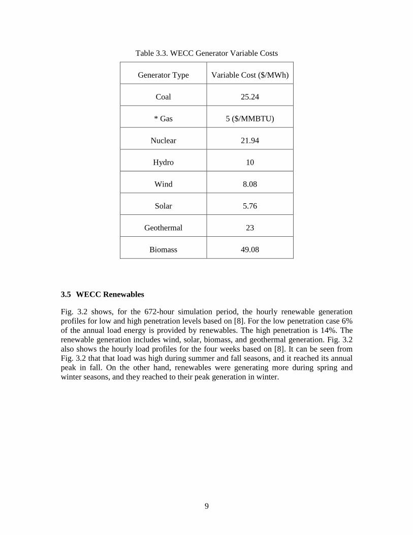
Table 3.3. WECC Generator Variable Costs

Generator Type Variable Cost ($/MWh)

Coal 25.24

* Gas 5 ($/MMBTU)

Nuclear 21.94

Hydro 10

Wind 8.08

Solar 5.76

Geothermal 23

Biomass 49.08

3.5 WECC Renewables

Fig. 3.2 shows, for the 672-hour simulation period, the hourly renewable generation profiles for low and high penetration levels based on [8]. For the low penetration case 6% of the annual load energy is provided by renewables. The high penetration is 14%. The renewable generation includes wind, solar, biomass, and geothermal generation. Fig. 3.2 also shows the hourly load profiles for the four weeks based on [8]. It can be seen from Fig. 3.2 that that load was high during summer and fall seasons, and it reached its annual peak in fall. On the other hand, renewables were generating more during spring and winter seasons, and they reached to their peak generation in winter.

10

Fig. 3.2. Renewables and load generation within the 672-hour simulation horizon.

0

20000

40000

60000

80000

100000

120000

140000

160000

0 168 336 504 672Time (hr)

Load (MW)

High Renewable (MW)

Low Renewable (MW)

11

4. Results

This section presents the results of different study cases for the PHS model, with and without cycling costs, and at the two renewable penetration levels. Results are compared with the base case, which has no PHS.

4.1 Conventional Generator Cycling Costs Included

Tables 4.1 and 4.2 show the results of the cases when cycling costs were considered for high and low renewables penetration levels respectively. The sub-optimized case uses equation (17), in which the pumping and generating times are provided by the PHS owner, but the PHS is dispatched by the ISO within those times. The optimized case uses equation (16), in which the PHS is both committed and dispatched by the ISO. This allows the PHS to flexibly change its pumping output to optimize the pumping and generating schedules.

Table 4.1. High Renewable with Cycling Cost Relative to No PHS Model Case

Renewables Penetration Level (%)

PHS Model Cycling Cost

Total System Cost ($)

Relative Reduction to Without PHS model

(%)

14 %

------------ Considered 1,043,140,602

------------

Sub-optimized Considered 1,040,535,361 0.25%

Fully- optimized Considered 1,006,555,221 3.51%

The results shown in Table 4.1 show a significant reduction in the sub- and fully-optimized operating costs relative to the case with no PHS. The relative reductions are considered significant since the total amount of storage, 3.02 GW/201 GWh, is low relative to the total renewable penetration of 29.14 GW. Table 4.1 shows that the PHS value (the difference between the operating cost and the cost without PHS) in the fully optimized case ($36,585,381) is much higher than its value in the sub-optimized case ($2,605,241). The total energy in the four-week period is 65.3 GWh, making the average energy costs $15.98/MWh for the case with no PHS, $15.94/MWh for the sub-optimized case, and $15.42/MWh for the fully- optimized case.

12

Table 4.2. Low Renewable with Cycling Cost Relative to No PHS Model Case

Renewables Penetration Level (%)

PHS Model Cycling Cost

Total System Cost ($)

Relative Reduction to Without PHS model

(%)

6 %

------------ Considered

1,133,079,936

------------

Sub-optimized Considered

1,129,850,198

0.29%

Fully- optimized Considered

1,094,895,374

3.08%

The lower renewable penetration results shown in Table 4.2 again show significant reductions in the sub- and fully optimized operating costs relative to the case without PHS. In this case the total renewable generation was 3.55 GW. Table 4.2 shows that the PHS value in the fully optimized case ($34,954,824) is much higher than its value in the sub-optimized case ($3,229,739). The average energy costs are $17.36/MWh for the case with no PHS, $17.31/MWh for the sub-optimized case, and $16.78/MWh for the fully- optimized case. Full optimization of PHS provided more operating cost savings in the higher renewables case than the lower renewables. However, the opposite happened with the sub-optimization of PHS in which the savings were more in the low renewables case. Thus, as the renewable penetration level increases, fully optimizing the PHS provides greater benefits to the system.

4.2 Conventional Generator Cycling Costs Not Included

Tables 4.3 and 4.4 show the results of the cases when cycling costs were not considered for high and low renewables penetration level respectively. Costs in each case are lower than the comparable Table 4.1 and 4.2 cases because cycling costs are not included. This comparison is discussed further in Tables 4.5 and 4.6. Both sub- and full-optimization still results in reduced operating costs, with full-optimization providing significantly higher reductions.

13

Table 4.3. High Renewable with No Cycling Cost Relative to No PHS Model Case

Renewables Penetration Level (%)

PHS Model Cycling Cost Total System Cost ($)

Relative Reduction to Without PHS

model (%)

14 %

------------ Not Considered

1,043,140,276

------------

Sub-optimized Not Considered

1,040,535,097

0.25%

Fully- optimized Not Considered

1,006,554,889

3.26%

Table 4.4. Low Renewable with No Cycling Cost Relative to No PHS Model Case

Renewables Penetration Level (%)

PHS Model Cycling Cost Total System Cost ($)

Relative Reduction to Without PHS

model (%)

6 %

------------ Not Considered 1,132,538,377 ------------

Sub-optimized Not Considered 1,129,850,088 0.24%

Fully- optimized Not Considered 1,094,895,249 3.09%

4.3 Effects of Including Conventional Generator Cycling Costs

Tables 4.5 and 4.6 detail the effects of considering cycling costs in scheduling generation with and without PHS. In all cases the total system cost is higher when cycling costs are considered, simply because those costs are added to the base operating cost. The differences are small, however, because for these cases the cycling costs were low compared to total operating costs. They did cause some changes in conventional generator and PHS scheduling, however, so they should be included in future studies.

14

Table 4.5. High Renewable, effects of considering cycling costs

Renewables Penetration Level (%)

PHS Model

Total System Cost ($), cycling cost

considered

Total System Cost ($), cycling cost not

considered

Difference in Cost

(%)

14 %

------------ 1,043,140,602

1,043,140,276 0.000031

Sub-optimized 1,040,535,361

1,040,535,097

0.000025

Fully- optimized 1,006,555,221 1,006,554,889

0.000033

Table 4.6. Low Renewable, effects of considering cycling costs

Renewables Penetration Level (%)

PHS Model

Total System Cost ($), cycling cost

considered

Total System Cost ($), cycling cost not

considered

Difference in Cost

(%)

6 %

------------

1,133,079,936

1,132,538,377 0.048

Sub-optimized

1,129,850,198

1,129,850,088 0.000010

Fully- optimized

1,094,895,374

1,094,895,249 0.000011

4.4 Solution Time and PHS Revenues

Table 4.7 presents the solving time and the PHS revenues for different cases. Table 4.7 shows that adding four PHS units with either sub- or full- optimization to the system increases the solving time between 121 and 223 percent. PHS revenue was calculated by subtracting the pumping cost from the generation revenue. As shown in Table X, the PHS generated revenue in all cases. The revenue may be supplemented by ancillary services markets or other incentives as renewable penetrations increase. Full-optimization increases revenues by more than ten times the sub-optimized revenues.

15

Table 4.7. Solving Time and PHS Revenues

Renewables Penetration Level (%)

PHS Model Cycling Cost Solving Time (sec) PHS Revenue ($)

14 % ------------ Considered 2045.14

Sub-optimized Considered 4119.78 3,096,400

Fully- optimized Considered 4674.73 43,554,546

6 % ------------ Considered 2045.04

Sub-optimized Considered 4727.19 3,172,113

Fully- optimized Considered 4770.74 44,637,755

14 % ------------ Not Considered 1947.48

Sub-optimized Not Considered 19514.52 3,096,376

Fully- optimized

Not Considered 5699.64 43,554,439

6 % ------------ Not Considered 1936.49

Sub-optimized Not Considered

7421.85

3,172,094

Fully- optimized

Not Considered

4371.45

50,276,202

16

4.5 Conventional Generator Cycling

Fig. 4.1 shows the operation of coal and gas generators for both low and high renewable penetrations with the fully-optimized PHS model and cycling costs considered. Most of the load and variable generation following is done by gas-fired generation, but in times of high load and high variability, coal-fired generation is also cycled. This again underscores the importance of considering cycling costs in dispatch calculations. Optimal dispatch of PHS also provides some of load and variable generation following that is needed, reducing the need for such cycling of conventional generation. Fig. 4.2 shows that more AS PHS units will be needed in the future to help with the cycling cost in reducing coal and gas generators cycling when high renewable penetrations are present in the system.

Fig. 4.1. Coal and gas generation for fully-optimized PHS and cycling cost considered under low and high renewables penetration level.

0

10000

20000

30000

40000

50000

60000

70000

0 168 336 504 672Time (hr)

Coal_LowRenewable (MW)

Gas_LowRenewable (MW)

Coal_HighRenewable (MW)

Gas_HighRenewable(MW)

17

Fig. 4.2. Coal and gas generation for no PHS and cycling cost considered under low and high renewables penetration level

0

10000

20000

30000

40000

50000

60000

70000

0 168 336 504 672Time (hr)

Coal_Low Renewable(MW)

Gas_Low Renewable(MW)

Coal_High Renewable(MW)

Gas_High Renewable(MW)

18

5. Conclusions

Simulations of the WECC system show that the conventional sub-optimized case, in which pumping and generation schedules are set by the PHS owner, provides revenue for the PHS owner and reduced system operating costs in both the 6% and 14% renewable penetration cases. The full optimization technique presented in section 2 provides a significant, greater than ten-fold, increase in PHS revenue and decrease in operating cost for all cases.

As renewable penetrations increase, conventional generation will cycle more to follow the variations in renewables. The cost associated with conventional generator cycling was estimated and included in the simulations. While this resulted in a very small change in total operating cost, it did change the dispatch of the generators. PHS mitigated some of the conventional generator cycling.

Increasing the penetration level of renewables increased the complexity of the system, and resulted in higher solution times. Optimizing PHS while considering the cycling cost reduces the total system operating cost and improves the DA market operation. Full optimization of AS PHS while considering the cycling cost resulted in the best total system cost savings, solving time, and PHS revenues. As renewable penetrations increase, more AS PHS can provide fast ramping to follow renewable variations and thus reduce the cycling of coal and gas generators.

19

6. Future Work

The proposed model in this paper will be extended to address modeling AS PHS, both open- and closed-loop, in real-time. The model will be applied on a large-scale system while considering the full-optimization case since none of the ISOs now fully optimize PHS in the real-time market.

A study for penetration levels of renewables higher than the ones presented in this paper, while considering the proposed CO2 emissions standards by the US Environmental Protection Agency (EPA) will be presented in future work.

PHS, especially with its AS capability, will have other applications in the future such as voltage control. A pricing structure will be developed to show the benefit of PHS in this and other ancillary services.

As penetrations of AS PHS increase, comparing modeling the PHS commitment in unit level (as it is modeled today) and plant level will be important to obtain faster convergence times when solving the mixed-integer programming (MIP) problem for unit commitment in the DA market. MIP problems involve the optimization of a linear objective function, subject to linear equality and inequality constraints. Some or all of the variables are required to be integer. One of the main factors that affects the performance of MIP is the number of binary variables and the constraints associated with them [14]. Therefore reducing the computation time and memory size allows more complexity to be added into the UC in the future, such as increasing the number of PHS plants [14]. This idea was based on [14], which provided a new plant level commitment model for FS PHS. The work in [14] has not been published yet.

20

References

[1] E. Ela, B. Kirby, A. Botterud, C. Milostan, I. Krad, and V. Koritarov (2013, Jul.). The Role of Pumped Storage Hydro Resources in Electricity Markets and System Operation. National Renewable Energy Laboratory, Denver, CO. [Online]. Available: http://www.nrel.gov/docs/fy13osti/58655.pdf

[2] Energy Storage Association (June 07). “Pumped Hyroelectric Storage”. [Online]. Available: http://energystorage.org/energy-storage/technologies/pumped-hydroelectric-storage

[3] V. Koritarov, T. Veselka, J. Gasper, B. Bethke, A. Botterud, J. Wang, M. Mahalik, Z. Zhou, and C. Milostan, “Modeling and Analysis of Value of Advanced Pumped Storage Hydropower in the United States” Argonne National Laboratory, Lemont, IL, Final Report, ANL/DIS-14/7, June. 2014.

[4] National Hydro Association (June 08). “Challenges and Opportunities for New Pumped Storage Development”. [Online]. Available: http://www.hydro.org/wpcontent/uploads/2014/01/NHA_PumpedStorage_071212b12.pdf

[5] E. Ela and V. Koritarov (2014, Jul.). Quantifying the Operational Benefits of Conventional and Advanced Pumped Storage Hydro on Reliability and Efficiency, Denver, CO. [Online]. Available: http://www.nrel.gov/docs/fy14osti/60806.pdf

[6] S. Frank, I. Steponavice, and S. Rebennack, “Optimal Power Flow A Bibliographic Survey I”, Energy Systems, September 2012, Volume 3, Issue 3, pp 221-258.

[7] R. D. Zimmerman, C. E. Murillo-Sánchez, and R. J. Thomas, "MATPOWER: Steady-State Operations, Planning and Analysis Tools for Power Systems Research and Education," Power Systems, IEEE Transactions on, vol. 26, no. 1, pp. 12-19, Feb. 2011.

[8] J. E. Price, and J. Goodin, “Reduced Network Modeling of WECC as Market Design Prototype”, July 2011

[9] Z. Hu, "Optimal Generation Expansion Planning with Integration of Variable Renewables and Bulk Energy Storage Systems," Ph.D. dissertation, Dept. Electrical. Eng., Univ. Wichita State, Wichita, KS, 2013.

[10] MWH (June 08). “Tehnical Analysis of Pumped Storage and Integration with Wind Power in the Pacific Northwest”. [Online]. Available: http://www.hydro.org/wp-content/uploads/2011/07/PS-Wind-Integration-Final-Report-without-Exhibits-MWH-3.pdf

21

[11] N. Kumar and P. Besuner, S. Lefton, D. Agan, and D. Hilleman (2012, Apr.). Power Plant Cycling Costs, Denver, CO. [Online]. Available: http://www.nrel.gov/docs/fy12osti/55433.pdf

[12] Carlos E. Murillo-Sanchez, R. D. Zimmerman, C. E., C. Lindsay Anderson, and Robert J. Thomas, Secure Planning and Operations of Systems with Stochastic Sources, Energy Storage, and Active Demand," IEEE Transactions on Smart Grid, vol. 4, no. 4, Dec. 2013.

[13] H. Aburub and W. Jewell, "Optimal Generation Planning to Improve Storage Cost and System Conditions", IEEE Power and Energy Society General Meeting, Washigton, July 2014.

[14] H. Aburub and M. Jin, "A New Commitment Model for Pumped Storage Hydro Resources ", conference paper in preparation.

[15] Pacific Northwest National Laboratory (August 09). “Energy Storage for Power Systems Applications: A Regional Assessment for the Northwest Power Pool”. [Online].Available:http://www.pnl.gov/main/publications/external/technical_reports/PNNL-19300.pdf

Part II

Enhanced Pumped Hydro Storage Model for Real-Time Operations

Nan Li Kory W. Hedman

Arizona State University

For information about this project, contact Kory W. Hedman Arizona State University School of Electrical, Computer, and Energy Engineering P.O. BOX 875706 Tempe, AZ 85287-5706 Phone: 480 965-1276 Fax: 480 965-0745 Email: kory.hedman@asu.edu Power Systems Engineering Research Center The Power Systems Engineering Research Center (PSERC) is a multi-university Center conducting research on challenges facing the electric power industry and educating the next generation of power engineers. More information about PSERC can be found at the Center’s website: http://www.pserc.org. For additional information, contact: Power Systems Engineering Research Center Arizona State University 527 Engineering Research Center Tempe, Arizona 85287-5706 Phone: 480-965-1643 Fax: 480-965-0745 Notice Concerning Copyright Material PSERC members are given permission to copy without fee all or part of this publication for internal use if appropriate attribution is given to this document as the source material. This report is available for downloading from the PSERC website.

2015 Arizona State University. All rights reserved.

i

Table of Contents

Table of Contents ................................................................................................................. i

List of Figures .................................................................................................................... iii

List of Tables ..................................................................................................................... iv

Nomenclature ...................................................................................................................... v

1. Introduction ................................................................................................................... 1

1.1 Background ........................................................................................................... 1

1.2 Summary of Chapters ........................................................................................... 2

2. Evaluation of the Fixed-Speed and the Adjustable-Speed Pumped Hydro Storage Technologies in Systems with Renewable Resources .................................................. 3

2.1 Introduction .......................................................................................................... 3

2.2 Mathematical Modeling of Pumped Hydro Storage ............................................. 4

2.2.1 Traditional Fixed-Speed Pumped Hydro Storage ......................................... 4

2.2.2 Adjustable-Speed Pumped Hydro Storage .................................................... 5

2.3 Mathematical Formulations of the Two-Step Approach ...................................... 6

2.3.1 The First-Step and the 6-Hour Ahead Unit Commitment Model .................. 6

2.3.2 The Second-Step and the 6-Hour Dispatch Model ........................................ 8

2.4 Case Studies ........................................................................................................ 10

2.4.1 IEEE 118-Bus System ................................................................................. 10

2.4.2 Renewable Scenario Generation ................................................................. 10

2.4.3 Simulation Setup ......................................................................................... 11

2.4.4 The First-Step and the 6-Hour Ahead Unit Commitment ........................... 11

2.4.5 The Second-Step and the 6-Hour Dispatch ................................................. 12

2.5 Conclusion .......................................................................................................... 13

3. Enhanced Utilization of Pumped Hydro Storage in Power System Operation using Policy Functions.......................................................................................................... 15

3.1 Introduction ........................................................................................................ 15

3.2 Policy Functions and the Proposed Framework ................................................. 16

3.3 Simulation Setup ................................................................................................ 17

3.4 Day-Ahead Unit Commitment ........................................................................... 18

3.5 Stochastic Simulation and the 24-Hour Dispatch Model ................................... 20

3.6 Generating Policy Function Approximation ...................................................... 22

ii

3.6.1 Classification Model ................................................................................... 22

3.6.2 Hierarchical Classification .......................................................................... 23

3.6.3 Classification Algorithm ............................................................................. 24

3.7 Evaluation of the Performance of the PFA ......................................................... 25

3.8 Case Study and Result Analysis ......................................................................... 25

3.8.1 Data Preparation .......................................................................................... 25

3.8.2 Modeling of Renewable Scenarios .............................................................. 26

3.8.3 Construction of the Classifiers .................................................................... 26

3.8.4 Performance Evaluation of the Proposed PFA ............................................ 28

3.9 Conclusion and Future Work .............................................................................. 32

4. Conclusions ................................................................................................................. 34

References ......................................................................................................................... 35

iii

List of Figures

Fig. 3.1. Overview of the proposed approach ................................................................... 17

Fig. 3.2. Flowchart for the simulation process.................................................................. 18

Fig. 3.3. Illustration of the classifier ................................................................................. 23

Fig. 3.4. Illustration of the hierarchical class structure ..................................................... 24

Fig. 3.5. Relative performance of the proposed PFA based approach .............................. 31

iv

List of Tables

Table 2.1. Parameters Used for the PHS Units ................................................................. 10

Table 2.2. System Results for the 6-Hour Ahead Unit Commitment ............................... 12

Table 2.3. Average Regulation Reserve Capacities Scheduled for the Fixed-Speed and the Adjustable-Speed PHS in Each Time Period .................................................................... 12

Table 2.4. Expected System Results for the 6-hour Dispatch Problem ............................ 13

Table 2.5. Expected Total Regulation Reserves Provided by the Fixed-Speed and Adjustable-Speed PHS in the 6-Hour Dispatch Problem ................................................. 13

Table 2.6. Statistical Description of the Total System Cost in the 6-Hour Dispatch Problem ($) ....................................................................................................................... 13

Table 3.1. Summary of the Input Attributes to the Classifier ........................................... 23

Table 3.2. Summary of the Parameters for the PHS ......................................................... 26

Table 3.3. Discretization of the Generation/Pumping Capacity of the PHS ..................... 27

Table 3.4. Summary of the Final Parameters Obtained by Grid-Search .......................... 28

Table 3.5. Accuracies Estimated for Each Classifier using 10-Fold Cross-Validation .... 28

Table 3.6. Expected System Results for each Method...................................................... 29

Table 3.7. Cost Savings by Using the Proposed PFA Approach ...................................... 29

Table 3.8. Average Computational Time for the Fixed-Schedule and the Policy Function Based Approach (s) ........................................................................................................... 31

v

Nomenclature

ADRRC Average down regulation reserve capacity

AURRC Average up regulation reserve capacity

𝑏 Index of energy storage units

𝑐 Index of contingencies

𝑐𝑔𝑙 (𝑐𝑏𝑙 ) Slope for segment l of piecewise linear cost function for generator g (energy storage b)

𝑐𝑏𝑖𝐿𝐿𝐿 Cost to violate the lower proxy limit determined for energy storage b in period t

𝐶𝑔 (𝐶𝑏) Variable cost function for generator g (energy storage b)

𝑐𝑔𝑁𝐿 (𝑐𝑏𝑁𝐿) No load cost for generator g (energy storage b)

𝑐𝑔𝑅 (𝑐𝑏𝑅) Ramping cost for generator g (energy storage b)

𝑐𝑔𝑆𝑆 (𝑐𝑏𝑆𝑆) Startup cost for generator g (energy storage b)

𝑐𝑏𝑖𝑆𝑈 Cost to violate the upper proxy limit determined for energy

storage b in period t

𝑑𝑠𝑖 Real power demand at node n in period t

𝐷𝐷𝑔 Minimum down time for unit g

𝐸𝑏𝑖 Storage level of the energy storage unit b in period t

𝐸𝑏,𝑖𝐿𝐿𝐿 Lower proxy limit determined by for energy storage b in

period t

𝐸𝑏𝑀𝑖𝑠 Minimum storage capacity of energy storage b

𝐸𝑏𝑀𝑠𝑠 Maximum storage capacity of energy storage b

𝐸𝑏,𝑖𝑆𝑈 Upper proxy limit determined by for energy storage b in

period t

𝐶𝑅𝑅 Number of attributes used for the base learners (decision trees) in a random forest classifier.

vi

g Index of generators

k Index of transmission lines

l Index of line segments of the piecewise linear function

L Number of line segments of the piecewise linear function

m Index for motors at PHS facility b

MILP Mixed-integer linear programming

n Index of buses

𝑁𝐸𝑆 Number of energy storage units

𝑁𝑇 Number of time periods

Nt Number of base learners (decision trees) used in a random forest classifier

𝑃𝑔𝑖 Power output of generator g in period t

𝑃�𝑔𝑖 Desired dispatch point for generator g in period t, determined by previous generation scheduling stage

𝑃𝑘𝑖 Real power flow on transmission line k in period t

𝑃𝑏𝐼𝑠_𝑒𝑠 Maximum pumping power for each motor at pumped hydro

storage facility b

𝑃𝑏𝑖𝐼𝑠 Power absorbed by energy storage unit b in period t

𝑃𝑏𝐼𝑠_𝑠𝑠𝑠

Maximum power absorption for energy storage b

𝑃𝑏𝐼𝑠_min

Minimum power absorption for energy storage b

𝑃𝑔𝑀𝑠𝑠 Maximum real power output for generator g

𝑃𝑘𝑀𝑠𝑠 Maximum MVA rating for transmission line k

𝑃𝑔𝑀𝑖𝑠 Minimum real power output for generator g

𝑃𝑏𝑂𝑢𝑖_𝑠𝑠𝑠

Maximum power output for energy storage b

𝑃𝑏𝑂𝑢𝑖_min

Minimum power output for energy storage b

vii

𝑃𝑏𝑖𝑂𝑢𝑖 Power generated by energy storage unit b in period t

𝑃�𝑏𝑖𝑂𝑢𝑖 Scheduled generation output for energy storage b in period t, determined from previous generation scheduling stage

𝑃𝐿𝑖𝑊𝑖𝑠𝑑 Power output for wind generator w in period t

PFA Policy function approximation

PHS Pumped hydro storage

𝑄𝑖𝑅+_𝑀𝑠𝑠

Maximum up regulation reserve provided by any single generating resource in period t

𝑄𝑖𝑅−_𝑀𝑠𝑠

Maximum down regulation reserve provided by any single generating resource in period t

𝑄𝑖𝑆_𝑀𝑠𝑠

Maximum spinning reserve provided by any single generating resource in period t

𝑟𝑔𝑖𝑆 (𝑟𝑏𝑖𝑆 ) Spinning reserve provided by generator g (energy storage b) in period t

�̅�𝑔𝑖𝑆 (�̅�𝑏𝑖𝑆 ) Scheduled spinning reserve for generator g (energy storage b) in period t, determined by previous generation scheduling stage

𝑟𝑔𝑖𝑅+ (𝑟𝑏𝑖𝑅+) Up regulation reserve provided by generator g (energy storage b) in period t

�̅�𝑔𝑖𝑅+ (�̅�𝑏𝑖𝑅+) Scheduled up regulation reserve for generator g (energy storage b) in period t, determined by previous generation scheduling stage

𝑟𝑔𝑖𝑅− (𝑟𝑏𝑖𝑅−) Down regulation reserve provided by generator g (energy storage b) in period t

�̅�𝑔𝑖𝑅− (�̅�𝑏𝑖𝑅−) Scheduled down regulation reserve for generator g (energy storage b) in period t, determined by previous generation scheduling stage

𝑅𝑔𝑆𝑔 Maximum shut-down ramp rate for generator g

𝑅𝑔𝑆𝑆 Maximum start-up ramp rate for generator g

𝑅𝑔𝑁𝑆 (𝑅𝑏𝑁𝑆) Maximum non-spinning reserve ramp rate for generator g (energy storage b)

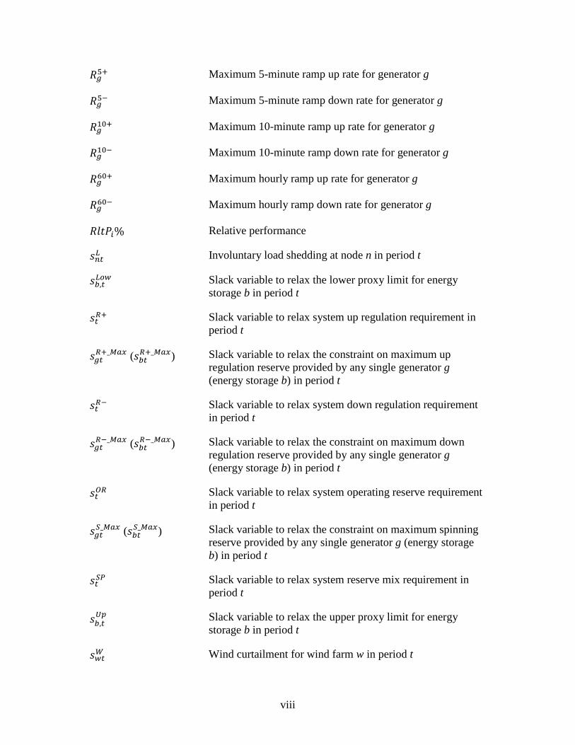
viii

𝑅𝑔5+ Maximum 5-minute ramp up rate for generator g

𝑅𝑔5− Maximum 5-minute ramp down rate for generator g

𝑅𝑔10+ Maximum 10-minute ramp up rate for generator g

𝑅𝑔10− Maximum 10-minute ramp down rate for generator g

𝑅𝑔60+ Maximum hourly ramp up rate for generator g

𝑅𝑔60− Maximum hourly ramp down rate for generator g

𝑅𝑅𝑅𝑃𝑖% Relative performance

𝑠𝑠𝑖𝐿 Involuntary load shedding at node n in period t

𝑠𝑏,𝑖𝐿𝐿𝐿 Slack variable to relax the lower proxy limit for energy

storage b in period t

𝑠𝑖𝑅+ Slack variable to relax system up regulation requirement in period t

𝑠𝑔𝑖𝑅+_𝑀𝑠𝑠 (𝑠𝑏𝑖

𝑅+_𝑀𝑠𝑠) Slack variable to relax the constraint on maximum up regulation reserve provided by any single generator g (energy storage b) in period t

𝑠𝑖𝑅− Slack variable to relax system down regulation requirement in period t

𝑠𝑔𝑖𝑅−_𝑀𝑠𝑠 (𝑠𝑏𝑖

𝑅−_𝑀𝑠𝑠) Slack variable to relax the constraint on maximum down regulation reserve provided by any single generator g (energy storage b) in period t

𝑠𝑖𝑂𝑅 Slack variable to relax system operating reserve requirement in period t

𝑠𝑔𝑖𝑆_𝑀𝑠𝑠 (𝑠𝑏𝑖

𝑆_𝑀𝑠𝑠) Slack variable to relax the constraint on maximum spinning reserve provided by any single generator g (energy storage b) in period t

𝑠𝑖𝑆𝑃 Slack variable to relax system reserve mix requirement in period t

𝑠𝑏,𝑖𝑆𝑈 Slack variable to relax the upper proxy limit for energy

storage b in period t

𝑠𝐿𝑖𝑊 Wind curtailment for wind farm w in period t

ix

t Index of time periods

𝑢𝑔𝑖 Binary unit commitment variable for generator g in period t (0 down, 1 online)

𝑢�𝑔𝑖 Scheduled commitment status for generator g in period t, determined by previous generation scheduling stage (0 down, 1 online)

UC Unit commitment

𝑈𝐷𝑔 Minimum up time for generator g

𝑣𝑔𝑖 Startup variable for generator g in period t (1 for startup, 0 otherwise)

�̅�𝑔𝑖 Scheduled startup for generator g in period t, determined by previous generation scheduling stage (1 for startup, 0 otherwise)

w Index of wind generators

𝑤𝑔𝑖 Shutdown variable for generator g in period t (1 for shutdown, 0 otherwise)

𝑤�𝑔𝑖 Scheduled shutdown for generator g in period t, determined by previous generation scheduling stage (1 for shutdown, 0 otherwise)

𝑧𝑏,𝑠,𝑖𝐼𝑠 Binary variable for the mth motor at the pumped hydro

storage facility b in period t (1 for consumption, 0 for idle)

𝑧𝑏𝑖𝐼𝑠 Binary variable for energy storage b in period t (1 for consumption, 0 for idle)

𝑧𝑏𝑖𝑂𝑢𝑖 Binary variable for energy storage b in period t (1 for production, 0 for idle)

𝛼𝑏𝑅 Minimum duration of time (hour) that the regulation reserve have to be maintained by energy storage b

𝛼𝑏𝑆 Minimum duration of time (hour) that the spinning reserve have to be maintained by energy storage b

𝜃𝑘𝑖+ Bus angle for the “from” bus of line k

𝜃𝑘𝑖− Bus angle for the “to” bus of line k

x

𝜂𝑏𝐼𝑠 Efficiency of the absorbing cycle of energy storage unit g

𝜂𝑏𝑂𝑢𝑖 Efficiency of the generating cycle of energy storage unit g

𝛿𝑘+(𝑚) For any transmission line k with “to” bus n

𝛿𝑘−(𝑚) For any transmission line k with “from” bus n

Ω𝐺 Set of conventional generators

Ω𝐺𝑠 Set of slow-start generators

Ω𝐺𝑓 Set of fast-start generators

∀(𝑚) For any generating unit at bus n

1

1. Introduction

1.1 Background

Due to the increasing environmental concerns and the need for a more sustainable power grid, power systems have seen a fast expansion of renewable resources in recent years. In the U.S, thirty states have enforced Renewable Portfolio Standards (RPS) or other mandated renewable capacities policies by January 2012. In California, the RPS requires that electric utilities should have 33% of their retail sales derived from eligible renewable energy resources by 2020 [4]. By the end of 2012, 60 GW of wind power capacity and 7.2 GW of solar power capacity have been installed in the U.S. [5]. The growing renewable penetration has increased the challenges to balance load with generation and to maintain the reliability of the system. To meet the stringent ramping requirement, more flexible resources are needed in the system.

Driven by the need to integrate high penetration levels of renewable resources and to reduce the costs for serving peak demands, recent interests have been focused on energy storage technologies. Energy storage can shift energy from peak-demand hours to off-peak-demand hours, or absorb excess renewable energy to provide it back to the grid when desired. The fast-ramping capability also makes energy storage a competitive resource to balance the variability and uncertainty in renewable generation. By using energy storage, the cycling of thermal units can be reduced, which is an advantage since many thermal units are not designed to be ramped up and down frequently [6].

As the most commercially matured large-scale energy storage technology, pumped hydro storage (PHS) has the largest installed capacity around the world, which is about 127 GW by 2010 [7]. Compared with other storage technologies, the PHS has the advantages of low capital cost, low maintenance cost and long life expectancies. Traditionally, studies are focused on the price-arbitrage value of PHS [8]-[10]. With the fast expansion of renewable generation during the last decade, new interests have been spent on the application of the PHS to facilitate the integration high levels of renewable resources [11]-[14].

While there are growing interests in energy storage in recent years, existing energy management systems and market management systems do not make full use of the flexibility of storage. One common approach for the utilization of storage is to determine schedules for a future time horizon based on a prior look-ahead time stage. The production and consumption schedule may then be fixed during this time, with limited adjustments. One example of such a strategy is peak shaving. Such approaches do not fully utilize the flexibility of storage as the actual characteristics of the storage are not fully modeled when solving (simultaneously) for the generation dispatch schedule across multiple time horizons while also accounting for uncertainties. With the introduction of high levels of variable renewable resources, it is much more advantageous to operate energy storage with more flexibility.

In this report, the challenges associated with utilizing the PHS in real-time operation are addressed. Distinct from thermal units, the dispatch of energy storage is constrained by their storage levels. The operation of the PHS in current stage has a large impact on the

2

future value of the resource at a later time stage. An inappropriate decision made for the PHS in the current time period could potentially result in insufficient capacity to produce or consume in future time periods. To improve the utilization of the PHS, a policy function based approach is proposed in the report. The proposed approach is aimed at improving the utilization of the PHS in real-time operations while having minimal added computational difficulty to the existing energy and market management systems.

At the same time, the report investigates two types of prevailing PHS technologies, namely the traditional fixed-speed technology and the more advanced adjustable-speed technology. Mathematical models are developed for the two PHS technologies. A two-step approach is proposed to simulate the scheduling and deployment of regulation reserves in systems with renewable resources. The capability of the two PHS technologies to provide regulation reserves are evaluated and compared using the proposed two-step approach.

1.2 Summary of Chapters

This report is structured as follows. In chapter 2, mathematical models are developed for the fixed-speed PHS and the adjustable-speed PHS. A two-step approach is proposed to evaluate and compare the attractiveness of the two PHS technologies in managing the renewable uncertainties in the system.

In chapter 3, a policy function based approach is proposed to enhance the utilization of the PHS in real-time operation. A classification algorithm is used to generate the policy function. The performance of the policy function based approach is compared with other benchmark approaches.

In chapter 4, the conclusions to this report are presented.

3

2. Evaluation of the Fixed-Speed and the Adjustable-Speed Pumped Hydro Storage Technologies in Systems with Renewable Resources

In this chapter, two different PHS technologies are studied, namely the traditional fixed-speed technology and the adjustable-speed technology. The technology principles and operational characteristics are introduced. Mathematical models are developed for the two types of PHS technologies. The capabilities of the two PHS technologies to provide regulation reserves are evaluated and compared using a two-step approach.

2.1 Introduction

The first use of pumped hydroelectric energy storage can be traced back to 1890 in Italy and Switzerland. Today, there are more than two hundred PHS facilities in operation or under planning around the world. As the most widely used bulk energy storage, PHS technologies have been advanced significantly since their first introduction, such as the inclusion of the use of reversible pump-turbines, the integration of power electronic devices, and the improvement of energy-conversion efficiencies. Since the 1990s, a newer PHS technology has been developed and used in commercial operation, which is named the adjustable-speed PHS technology.

For traditional fixed-speed technology, the input power is fixed during the pumping process and the fixed-speed PHS can only provide regulation reserves in the generation mode. However, the adjustable-speed technology provides the PHS the capability to adjust its input power in the pumping mode. With this improvement, the adjustable-speed PHS is able to provide regulation reserves in both the pumping and generation mode. By using the adjustable-speed design, round-trip efficiencies are also improved for the PHS [15]. As renewable penetration increases, the capability to provide regulation reserves in both the pumping and generation model will make the adjustable-speed PHS a more valuable generation resource. Globally, there are about 270 PHS stations currently either in operation or under construction. Among them, 36 facilities are equipped with adjustable-speed machines. Most of the existing adjustable-speed PHS projects are located in China, Japan, India and Europe. In the U.S., none of the existing PHS facilities are equipped with adjustable-speed units. However, several projects in the design or planning stage in the U.S. are considering and evaluating the use of adjustable-speed design.

In this chapter, fixed-speed PHS technologies and adjustable-speed PHS technologies are studied. The technology principles are introduced for the two PHS designs. Mathematical models are developed for the two PHS technologies. A two-step approach is proposed to evaluate and compare the benefits of using the fixed-speed and the adjustable-speed PHS in systems with renewable resources.

4

2.2 Mathematical Modeling of Pumped Hydro Storage

In this subsection, mathematical models are derived for the PHS with fixed-speed design and adjustable-speed design. The focus of the formulations is to capture the differences in the capability of the two PHS technologies to provide ancillary services.

2.2.1 Traditional Fixed-Speed Pumped Hydro Storage

In the U.S., most of the traditional PHS facilities use a pump-turbine equipment design named reversible single-stage Francis pump-turbine, where the machine works as a pump in one direction and acts as a turbine in the other [16]. For this technology, the input power is fixed and cannot be varied in the pumping mode. Therefore, the pumping power for the PHS with fixed-speed technology is either 0 or 100% of the maximum pumping power rating. Depending on the design of the plant, some fixed-speed PHS facilities may be able to increase pumping power in a “block” manner, which is to turn on the motors one by one to increase the pumping power. The mathematical model for a PHS facility with a traditional fixed-speed design can be formulated as

𝑟𝑏𝑖𝑆 + 𝑟𝑏𝑖𝑅+ ≤ 𝑃𝑏𝑂𝑢𝑖_𝑠𝑠𝑠 − 𝑃𝑏𝑖𝑂𝑢𝑖 + 𝑃𝑏𝑖𝐼𝑠,∀𝑏, 𝑅 (2.1)

𝑟𝑏𝑖𝑅+ ≤ 𝑃𝑏𝑂𝑢𝑖_𝑠𝑠𝑠(1 − 𝑧𝑏𝑖𝐼𝑠) − 𝑃𝑏𝑖𝑂𝑢𝑖,∀𝑏, 𝑅 (2.2)

𝛼𝑏𝑆𝑟𝑏𝑖𝑆 + 𝛼𝑏𝑅𝑟𝑏𝑖𝑅+ ≤ 𝜂𝑏𝑂𝑢𝑖(𝐸𝑏𝑖 − 𝐸𝑏𝑀𝑖𝑠),∀𝑏, 𝑅 (2.3)

𝑟𝑏𝑖𝑅− ≤ 𝑃𝑏𝑖𝑂𝑢𝑖,∀𝑏, 𝑅 (2.4)

𝐸𝑏𝑖 = 𝐸𝑏,𝑖−1 + 𝑃𝑏𝑖𝐼𝑠𝜂𝑏𝐼𝑠 − 𝑃𝑏𝑖𝑂𝑢𝑖 𝜂𝑏𝑂𝑢𝑖⁄ ,∀𝑏, 𝑅 (2.5)

𝑃𝑏𝑂𝑢𝑖_𝑠𝑖𝑠𝑧𝑏𝑖𝑂𝑢𝑖 ≤ 𝑃𝑏𝑠𝑖𝑂𝑢𝑖 ≤ 𝑃𝑏

𝑂𝑢𝑖_𝑠𝑠𝑠𝑧𝑏𝑖𝑂𝑢𝑖,∀𝑏, 𝑅 (2.6)

𝑃𝑏𝑖𝐼𝑠 = 𝑃𝑏𝐼𝑠_𝑒𝑠 ∑ 𝑧𝑏,𝑠,𝑖

𝐼𝑠𝑠 ,∀𝑏, 𝑅 (2.7)

𝐸𝑏𝑀𝑖𝑠 ≤ 𝐸𝑏𝑖 ≤ 𝐸𝑏𝑀𝑠𝑠,∀𝑏, 𝑅 (2.8)

𝑧𝑏𝑖𝐼𝑠 ≥ 𝑧𝑏,𝑠,𝑖𝐼𝑠 ,∀𝑏,𝑚, 𝑅 (2.9)

𝑧𝑏𝑖𝑂𝑢𝑖 + 𝑧𝑏𝑖𝐼𝑠 ≤ 1,∀𝑏, 𝑅 (2.10)

𝑧𝑏,𝑠,𝑖𝐼𝑠 , 𝑧𝑏𝑖𝑂𝑢𝑖, 𝑧𝑏𝑖𝐼𝑠 ∈ {0,1},∀𝑏,𝑚, 𝑅. (2.11)

In the above formulation, constraints (2.1)-(2.4) represent the ancillary serves provided by the PHS. Constraint (2.1) and (2.2) indicates that if the PHS is in the idle or generation mode, the sum of spinning and up regulation reserves the PHS can provide is 𝑃𝑏

𝑂𝑢𝑖_𝑠𝑠𝑠 −𝑃𝑏𝑖𝑂𝑢𝑖; if the PHS is in the pumping mode, then the PHS cannot provide up regulation reserve. The maximum spinning reserve the PHS can provide in the pumping mode is 𝑃𝑏𝑂𝑢𝑖_𝑠𝑠𝑠 + 𝑃𝑏𝑖𝐼𝑠, which means the PHS can stop pumping and transition to generation

5

mode to provide spinning reserve. Constraint (2.4) indicates that the fixed-speed PHS can only provide down regulation reserves in the generation mode. Constraints (2.3) guarantees that the PHS has enough energy to provide spinning and regulation reserves. Constraint (2.5) is the energy balance constraint and (2.6) represent the limits on the generation power. The limit on the pumping power is presented in (2.7). In (2.7), 𝑃𝑏

𝐼𝑠_𝑒𝑠 is the maximum pumping power rating for each motor in the PHS facility b, and m is the index for the motors at the facility b. This constraint indicates that if multiple motors are installed at the PHS facility, the pumping power can be increased in a “block” manner. Constraint (2.8) represents the minimum and maximum capacities of the water reservoir of the PHS facility. Constraint (2.9) and (2.10) formulate the relationships between the binary variables. Constraint (2.11) indicates that 𝑧𝑏,𝑠,𝑖

𝐼𝑠 , 𝑧𝑏𝑖𝑂𝑢𝑖 and 𝑧𝑏𝑖𝐼𝑠 are binary variables.

2.2.2 Adjustable-Speed Pumped Hydro Storage

The first adjustable-speed PHS facility was built by Tokyo Electric in Japan in 1990 [17]. One common design for the adjustable-speed PHS is to use a double-fed induction motor-generator. Compared to traditional fixed-speed design, the primary advantage of adjustable-speed technology is that the input power can be varied in the pumping mode. The mathematical model for a PHS facility with an adjustable-speed design is formulated as

𝑟𝑏𝑖𝑆 + 𝑟𝑏𝑖𝑅+ ≤ 𝑃𝑏𝑂𝑢𝑖_𝑠𝑠𝑠 − 𝑃𝑏𝑖𝑂𝑢𝑖 + 𝑃𝑏𝑖𝐼𝑠,∀𝑏, 𝑅 (2.12)

𝛼𝑏𝑆𝑟𝑏𝑖𝑆 + 𝛼𝑏𝑅𝑟𝑏𝑖𝑅+ ≤ 𝜂𝑏𝑂𝑢𝑖(𝐸𝑏𝑠𝑖 − 𝐸𝑏𝑀𝑖𝑠),∀𝑏, 𝑅 (2.13)

𝑟𝑏𝑖𝑅− ≤ 𝑃𝑏𝐼𝑠_𝑠𝑠𝑠 − 𝑃𝑏𝑖𝐼𝑠 + 𝑃𝑏𝑖𝑂𝑢𝑖,∀𝑏, 𝑅 (2.14)

𝛼𝑏𝑅𝑟𝑏𝑖𝑅− ≤ (𝐸𝑏𝑀𝑠𝑠 − 𝐸𝑏,𝑖)/𝜂𝑏𝐼𝑠,∀𝑏, 𝑅 (2.15)

𝐸𝑏𝑖 = 𝐸𝑏,𝑖−1 + 𝑃𝑏𝑖𝐼𝑠𝜂𝑏𝐼𝑠 − 𝑃𝑏𝑖𝑂𝑢𝑖 𝜂𝑏𝑂𝑢𝑖⁄ ,∀𝑏, 𝑅 (2.16)

𝑃𝑏𝑂𝑢𝑖_𝑠𝑖𝑠𝑧𝑏𝑖𝑂𝑢𝑖 ≤ 𝑃𝑏𝑠𝑖𝑂𝑢𝑖 ≤ 𝑃𝑏

𝑂𝑢𝑖_𝑠𝑠𝑠𝑧𝑏𝑖𝑂𝑢𝑖,∀𝑏, 𝑅 (2.17)

𝑃𝑏𝐼𝑠_𝑠𝑖𝑠𝑧𝑏𝑖𝐼𝑠 ≤ 𝑃𝑏𝑖𝐼𝑠 ≤ 𝑃𝑏

𝐼𝑠_𝑠𝑠𝑠𝑧𝑏𝑖𝐼𝑠,∀𝑏, 𝑅 (2.18)

𝑧𝑏𝑖𝑂𝑢𝑖 + 𝑧𝑏𝑖𝐼𝑠 ≤ 1,∀𝑏, 𝑅 (2.19)

𝐸𝑏𝑀𝑖𝑠 ≤ 𝐸𝑏𝑖 ≤ 𝐸𝑏𝑀𝑠𝑠,∀𝑏, 𝑅 (2.20)

𝑧𝑏𝑖𝑂𝑢𝑖, 𝑧𝑏𝑖𝐼𝑠 ∈ {0,1},∀𝑏, 𝑅. (2.21)

In the above formulation, constraints (2.12)-(2.15) represent the ancillary services provided by the adjustable-speed PHS. Constraint (2.12)-(2.15) indicate that the regulation reserves can be provided in both the generation and pumping mode. The energy balance constraint is presented in (2.16). Constraints (2.17) and (2.18) represent the limits on the generation and pumping power of the PHS. Constraint (2.19) indicates

6

that the PHS can only be in one mode at the same time. The minimum and maximum limits on the water reservoir are presented in (2.20).

2.3 Mathematical Formulations of the Two-Step Approach

A two-step approach is proposed to evaluate the capability of the fixed-speed and the adjustable-speed PHS to provide regulation reserves. The proposed approach represents the scheduling and deployment of the regulation reserves. In the first-step, a unit commitment model is used to determine the generation and reserve schedules. In the second-step, a 6-hour dispatch model is used to simulate the activation of the regulation reserves. The mathematical models used in the two-step approach are described in the following subsections. It should be noted that the regulation reserve studied in this chapter can be more accurately categorized as the load following reserve product, since in this study, the regulation reserves are primarily used to address the renewable variability and uncertainty at 10-minute intervals. However, to keep the terminology consistent, the term “regulation reserve” are used instead of “load following reserves” in this chapter.

2.3.1 The First-Step and the 6-Hour Ahead Unit Commitment Model

A 6-hour ahead deterministic unit commitment (UC) problem is formulated in the first-step of the proposed approach. The UC represents a short-term generation scheduling problem, which is typically solved between the day-ahead UC and the real-time economic dispatch. The UC is formulated as a mixed integer linear program (MILP). The UC is modeled with 36 time periods, with each to be a 10-minute interval; note that a 10-minute interval was chosen since the wind data has a 10-minute resolution. Many real-time markets operate on a 5-minute basis; the proposed model can easily accommodate 5-minute intervals. The objective of the UC is to minimize the total system operating cost and the costs to correct system security violations. The system security violation costs include the costs to correct system involuntary load shedding and system reserve requirement violations. The complete formulation is shown in (2.22)-(2.47).

Minimize:

∑ ∑ �𝐶𝑔�𝑃𝑔𝑖� + 𝑐𝑔𝑁𝐿𝑢𝑔𝑖 + 𝑐𝑔𝑆𝑆𝑣𝑔𝑖�𝑖𝑔 + ∑ �𝑐𝑣𝑅+𝑠𝑖𝑅+ + 𝑐𝑣𝑅−𝑠𝑖𝑅− + 𝑐𝑣𝑆𝑃𝑠𝑖𝑆𝑃 + 𝑐𝑣𝑂𝑅𝑠𝑖𝑂𝑅�𝑖 +∑ ∑ 𝑐𝑣𝑅𝑠_Max�𝑠𝑔𝑖

𝑆_𝑀𝑠𝑠 + 𝑠𝑔𝑖𝑅+_𝑀𝑠𝑠 + 𝑠𝑔𝑖

𝑅−_𝑀𝑠𝑠�𝑖𝑔 + ∑ ∑ 𝑐𝑣𝑅𝑠_Max�𝑠𝑏𝑖𝑆_𝑀𝑠𝑠 + 𝑠𝑏𝑖

𝑅+_𝑀𝑠𝑠 +𝑖𝑏

𝑠𝑏𝑖𝑅−_𝑀𝑠𝑠� + ∑ ∑ 𝑐𝑣𝐿𝑠𝑠𝑖𝐿𝑖𝑠 (2.22)

Subject to:

∑ 𝑃𝑔𝑖∀𝑔(𝑠) + ∑ 𝑃𝑘𝑖𝑘∈𝛿+(𝑠) − ∑ 𝑃𝑘𝑖𝑘∈𝛿−(𝑠) + ∑ (𝑃𝑏𝑖𝑂𝑢𝑖 − 𝑃𝑏𝑖𝐼𝑠)∀𝑏(𝑠) = 𝑑𝑠𝑖 − 𝑠𝑠𝑖𝐿 −∑ (𝑃𝐿𝑖𝑊𝑖𝑠𝑑 − 𝑠𝐿𝑖𝑊 )∀𝐿(𝑠) ,∀𝑚, 𝑅 (2.23)

𝑃𝑘𝑖 − 𝐵𝑘(𝜃𝑘𝑖+ − 𝜃𝑘𝑖− ) = 0,∀𝑘, 𝑅 (2.24)

−𝑃𝑘𝑠𝑠𝑠 ≤ 𝑃𝑘𝑖 ≤ 𝑃𝑘𝑠𝑠𝑠 ,∀𝑘, 𝑅 (2.25)

7

𝑃𝑔𝑖 + 𝑟𝑔𝑖𝑅+ + 𝑟𝑔𝑖𝑆 ≤ 𝑃𝑔𝑠𝑠𝑠𝑢𝑔𝑖,∀𝑔, 𝑅 (2.26)

𝑃𝑔𝑠𝑖𝑠𝑢𝑔𝑖 ≤ 𝑃𝑔𝑖 − 𝑟𝑔𝑖𝑅−,∀𝑔, 𝑅 (2.27)

∑ 𝑣𝑔𝑔𝑖𝑔=𝑖−𝑆𝑇𝑔+1 ≤ 𝑢𝑔𝑖, ∀𝑔, 𝑅 ∈ �𝑈𝐷𝑔, … ,𝐷� (2.28)

∑ 𝑤𝑔𝑔𝑖𝑔=𝑖−𝑔𝑇𝑔+1 ≤ 1 − 𝑢𝑔𝑖, ∀𝑔, 𝑅 ∈ �𝐷𝐷𝑔, … ,𝐷� (2.29)

𝑣𝑔𝑖 − 𝑤𝑔𝑖 = 𝑢𝑔𝑖 − 𝑢𝑔,𝑖−1, ∀𝑔, 𝑅 (2.30)

𝑟𝑔𝑖𝑅+ ≤ 𝑅𝑔5+𝑢𝑔𝑖, 𝑟𝑔𝑖𝑅− ≤ 𝑅𝑔5−𝑢𝑔𝑖, ∀𝑔, 𝑅 (2.31)

𝑟𝑔𝑖𝑆 ≤ 𝑅𝑔10+𝑢𝑔𝑖,∀𝑔, 𝑅 (2.32)

𝑟𝑔𝑖𝑁𝑆 ≤ 𝑅𝑔𝑁𝑆(1 − 𝑢𝑔𝑖),∀𝑔, 𝑅 (2.33)

𝑃𝑔,𝑖 − 𝑃𝑔,𝑖−1 ≤ 𝑅𝑔10+𝑢𝑔,𝑖−1 + 𝑅𝑔𝑆𝑆𝑣𝑔𝑖,∀𝑔, 𝑅 (2.34)

𝑃𝑔,𝑖−1 − 𝑃𝑔,𝑖 ≤ 𝑅𝑔10−𝑢𝑔𝑖 + 𝑅𝑔𝑆𝑔𝑤𝑔𝑖,∀𝑔, 𝑅 (2.35)

∑ 𝑟𝑔𝑖𝑅+𝑔 + ∑ 𝑟𝑏𝑖𝑅+𝑏 ≥ 0.02∑ 𝑑𝑠𝑖𝑠 − 𝑠𝑖𝑅+,∀𝑅 (2.36)

∑ 𝑟𝑔𝑖𝑅−𝑔 + ∑ 𝑟𝑏𝑖𝑅−𝑏 ≥ 0.02∑ 𝑑𝑠𝑖𝑠 − 𝑠𝑖𝑅−,∀𝑅 (2.37)

𝑄𝑖𝑂𝑅 ≥ 𝑃𝑔𝑖 + 𝑟𝑔𝑖𝑆 ,∀𝑔, 𝑅 (2.38)

𝑄𝑖𝑂𝑅 ≥ 0.03∑ 𝑑𝑠𝑖𝑠 + 0.05∑ 𝑃𝐿𝑖𝑊𝑖𝑠𝑑𝐿 ,∀𝑅 (2.39)

∑ 𝑟𝑔𝑖𝑆𝑔 + ∑ 𝑟𝑏𝑖𝑆𝑏 + ∑ 𝑟𝑔𝑖𝑁𝑆𝑔 ≥ 𝑄𝑖𝑂𝑅 − 𝑠𝑖𝑂𝑅 ,∀𝑅 (2.40)

∑ 𝑟𝑔𝑖𝑆𝑔 + ∑ 𝑟𝑏𝑖𝑆𝑏 ≥ 0.5𝑄𝑖𝑂𝑅 − 𝑠𝑖𝑆𝑃,∀𝑅 (2.41)

𝑟𝑔𝑖𝑆 ≤ 𝑄𝑖𝑆_𝑀𝑠𝑠 − 𝑠𝑔𝑖

𝑆_𝑀𝑠𝑠 ,∀𝑔, 𝑅 (2.42)

𝑟𝑏𝑖𝑆 ≤ 𝑄𝑖𝑆_𝑀𝑠𝑠 − 𝑠𝑏𝑖

𝑆_𝑀𝑠𝑠,∀𝑏, 𝑅 (2.43)

𝑟𝑔𝑖𝑅+ ≤ 𝑄𝑖𝑅+_𝑀𝑠𝑠 − 𝑠𝑔𝑖

𝑅+_𝑀𝑠𝑠,∀𝑔, 𝑅 (2.44)

𝑟𝑏𝑖𝑅+ ≤ 𝑄𝑖𝑅+_𝑀𝑠𝑠 − 𝑠𝑏𝑖

𝑅+_𝑀𝑠𝑠,∀𝑏, 𝑅 (2.45)

𝑟𝑔𝑖𝑅− ≤ 𝑄𝑖𝑅−_𝑀𝑠𝑠 − 𝑠𝑔𝑖

𝑅−_𝑀𝑠𝑠,∀𝑔, 𝑅 (2.46)

𝑟𝑏𝑖𝑅− ≤ 𝑄𝑖𝑅−𝑀𝑠𝑠 − 𝑠𝑏𝑖

𝑅−_𝑀𝑠𝑠 ,∀𝑏, 𝑅 (2.47)

8

Constraint (2.23) guarantees the power balance at every bus. Constraint (2.24) represents the dc power flow on each line and (2.25) is the line-flow limit constraint. Limits on the power output for each generator are presented in (2.26) and (2.27). The minimum up and down time constraints are shown in (2.28)-(2.30). Constraints (2.31)-(2.33) represent the ramp rates for regulation, spinning and non-spinning reserves for the thermal units. The ramp rate constraints are shown in (2.34) and (2.35).

The system-wide reserve requirement constraints are presented in (2.36)-(2.47). The regulation reserve requirement is set to be 2% of the hourly load, as shown in (2.36) and (2.37). Constraints (2.38)-(2.40) require that the system operating reserve (sum of spinning and non-spinning reserves) should be greater or equal to the single largest generator contingency, or the NREL’s “3+5” reserve rule [18], whichever is greater. The NREL’s “3+5” reserve rule is used to address the renewable uncertainties. Constraint (2.41) indicates that half of the system operating reserve should come from spinning reserve. Constraint (2.42)-(2.47) limit the maximum spinning and regulation reserve that each unit can provide. Similar constraints are also used in [19] and [20]. If too much reserve is scheduled on a single unit, the reserves may not be deliverable due to transmission congestions. The use of constraints (2.42)-(2.47) in this work can be seen as a simple rule to improve the deliverability of the reserves. In constraints (2.42)-(2.47), it is required that the maximum reserve from any single resource should be less or equal to 50% of the reserve requirement. The reserve requirement constraints can be violated for a predetermined penalty price.

For the PHS, the model presented in the previous subsection is used. If the fixed-speed PHS is considered, constraints (2.1)-(2.11) are used in combination with the unit commitment model (2.22)-(2.47). If the adjustable-speed PHS is considered, constraints (2.12)-(2.21) are included in the unit commitment model.

2.3.2 The Second-Step and the 6-Hour Dispatch Model

In the second-step, a 6-hour dispatch problem is formulated to test the UC solution against a large number of wind scenarios. The scheduled regulation reserves are activated in the second-step to address the renewable uncertainties. For the 6-hour dispatch model, thirty-six time periods are included, with each time period representing a 10-minute interval. The 6-hour dispatch problem is an approximation to the real-time dispatch problem with the simplification that all the time periods are solved in one optimization program rather than using a rolling horizon approach; this horizon is chosen to approximate the benefits of adjustable speed PHS. The complete formulation of the 6-hour dispatch problem is presented in (2.48)-(2.70).

Minimize:

∑ ∑ �𝐶𝑔�𝑃𝑔𝑖� + 𝑐𝑔𝑁𝐿𝑢𝑔𝑖 + 𝑐𝑔𝑆𝑆𝑣𝑔𝑖�𝑖𝑔 + ∑ �𝑐𝑣𝑅+𝑠𝑖𝑅+ + 𝑐𝑣𝑅−𝑠𝑖𝑅− + 𝑐𝑣𝑆𝑃𝑠𝑖𝑆𝑃 + 𝑐𝑣𝑂𝑅𝑠𝑖𝑂𝑅�𝑖 +∑ ∑ 𝑐𝑣𝑅𝑠_Max𝑠𝑔𝑖

𝑆_𝑀𝑠𝑠𝑖𝑔 + ∑ ∑ 𝑐𝑣𝑅𝑠_Max𝑠𝑏𝑖

𝑆_𝑀𝑠𝑠𝑖𝑏 + ∑ ∑ 𝑐𝑣𝐿𝑠𝑠𝑖𝐿𝑖𝑠 (2.48)

Subject to:

9

∑ 𝑃𝑔𝑖∀𝑔(𝑠) + ∑ 𝑃𝑘𝑖𝑘∈𝛿+(𝑠) − ∑ 𝑃𝑘𝑖𝑘∈𝛿−(𝑠) + ∑ (𝑃𝑏𝑖𝑂𝑢𝑖 − 𝑃𝑏𝑖𝐼𝑠)∀𝑏(𝑠) = 𝑑𝑠𝑖 − 𝑠𝑠𝑖𝐿 −∑ (𝑃𝐿𝑖𝑊𝑖𝑠𝑑 − 𝑠𝐿𝑖𝑊 )∀𝐿(𝑠) ,∀𝑚, 𝑅 (2.49)

𝑃𝑘𝑖 − 𝐵𝑘(𝜃𝑘𝑖+ − 𝜃𝑘𝑖− ) = 0,∀𝑘, 𝑅 (2.50)

−𝑃𝑘𝑠𝑠𝑠 ≤ 𝑃𝑘𝑖 ≤ 𝑃𝑘𝑠𝑠𝑠 ,∀𝑘, 𝑅 (2.51)

𝑃𝑔𝑠𝑖𝑠𝑢𝑔𝑖 ≤ 𝑃𝑔𝑖 ≤ 𝑃𝑔𝑠𝑠𝑠𝑢𝑔𝑖 − 𝑟𝑔𝑖𝑆 ,∀𝑔, 𝑅 (2.52)

(𝑃�𝑔𝑖 − �̅�𝑔𝑖𝑅−)𝑢𝑔𝑖 ≤ 𝑃𝑔𝑖 ≤ (𝑃�𝑔𝑖 + �̅�𝑔𝑖𝑅+)𝑢𝑔𝑖,∀𝑔 ∈ 𝛺𝐺 , 𝑅 (2.53)

𝑟𝑔𝑖𝑆 ≤ 𝑅𝑔10+𝑢𝑔𝑖,∀𝑔, 𝑅 (2.54)

𝑃𝑔,𝑖 − 𝑃𝑔,𝑖−1 ≤ 𝑅𝑔10+𝑢𝑔,𝑖−1 + 𝑅𝑔𝑆𝑆𝑣𝑔𝑖,∀𝑔, 𝑅 (2.55)

𝑃𝑔,𝑖−1 − 𝑃𝑔,𝑖 ≤ 𝑅𝑔10−𝑢𝑔𝑖 + 𝑅𝑔𝑆𝑔𝑤𝑔𝑖,∀𝑔, 𝑅 (2.56)

𝑢𝑔𝑖 = 𝑢𝑔𝑖 , 𝑣𝑔𝑖 = 𝑣𝑔𝑖,𝑤𝑔𝑖 = 𝑤𝑔𝑖,∀𝑔 ∈ Ω𝐺 , 𝑅 (2.57)

𝑟𝑏𝑖𝑆 ≤ 𝑃𝑏𝑂𝑢𝑖_𝑠𝑠𝑠 − 𝑃𝑏𝑖𝑂𝑢𝑖 + 𝑃𝑏𝑖𝐼𝑠,∀𝑏, 𝑅 (2.58)

𝛼𝑏𝑆𝑟𝑏𝑖𝑆 ≤ 𝜂𝑏𝑂𝑢𝑖(𝐸𝑏𝑖 − 𝐸𝑏𝑀𝑖𝑠),∀𝑏, 𝑅 (2.59)

𝐸𝑏𝑖 = 𝐸𝑏,𝑖−1 + 𝑃𝑏𝑖𝐼𝑠𝜂𝑏𝐼𝑠 − 𝑃𝑏𝑖𝑂𝑢𝑖 𝜂𝑏𝑂𝑢𝑖⁄ ,∀𝑏, 𝑅 (2.60)

𝑃𝑏𝑂𝑢𝑖_𝑠𝑖𝑠𝑧𝑏𝑖𝑂𝑢𝑖 ≤ 𝑃𝑏𝑠𝑖𝑂𝑢𝑖 ≤ 𝑃𝑏

𝑂𝑢𝑖_𝑠𝑠𝑠𝑧𝑏𝑖𝑂𝑢𝑖,∀𝑏, 𝑅 (2.61)

𝑃𝑏𝐼𝑠_𝑠𝑖𝑠𝑧𝑏𝑖𝐼𝑠 ≤ 𝑃𝑏𝑖𝐼𝑠 ≤ 𝑃𝑏

𝐼𝑠_𝑠𝑠𝑠𝑧𝑏𝑖𝐼𝑠,∀𝑏, 𝑅 (2.62)

𝑃�𝑏𝑖𝐸𝑆 − �̅�𝑏𝑖𝑅− ≤ 𝑃𝑏𝑖𝐸𝑆 ≤ 𝑃�𝑏𝑖𝐸𝑆 + �̅�𝑔𝑖𝑅+,∀𝑏, 𝑅 (2.63)

𝑧𝑏𝑖𝑂𝑢𝑖 + 𝑧𝑏𝑖𝐼𝑠 ≤ 1,∀𝑏, 𝑅 (2.64)

𝐸𝑏𝑀𝑖𝑠 ≤ 𝐸𝑏𝑖 ≤ 𝐸𝑏𝑀𝑠𝑠,∀𝑏, 𝑅 (2.65)

𝑄𝑖𝑂𝑅 ≥ 𝑃𝑔𝑖 + 𝑟𝑔𝑖𝑆 ,∀𝑔, 𝑅 (2.66)

∑ 𝑟𝑔𝑖𝑆𝑔 + ∑ 𝑟𝑏𝑖𝑆𝑏 + ∑ 𝑟𝑔𝑖𝑁𝑆𝑔 ≥ 𝑄𝑖𝑂𝑅 − 𝑠𝑖𝑂𝑅 ,∀𝑅 (2.67)

∑ 𝑟𝑔𝑖𝑆𝑔 + ∑ 𝑟𝑏𝑖𝑆𝑏 ≥ 0.5𝑄𝑖𝑂𝑅 − 𝑠𝑖𝑆𝑃,∀𝑅 (2.68)

𝑟𝑔𝑖𝑆 ≤ 𝑄𝑖𝑆_𝑀𝑠𝑠 − 𝑠𝑔𝑖

𝑆_𝑀𝑠𝑠 ,∀𝑔, 𝑅 (2.69)

𝑟𝑏𝑖𝑆 ≤ 𝑄𝑖𝑆_𝑀𝑠𝑠 − 𝑠𝑏𝑖

𝑆_𝑀𝑠𝑠,∀𝑏, 𝑅 (2.70)

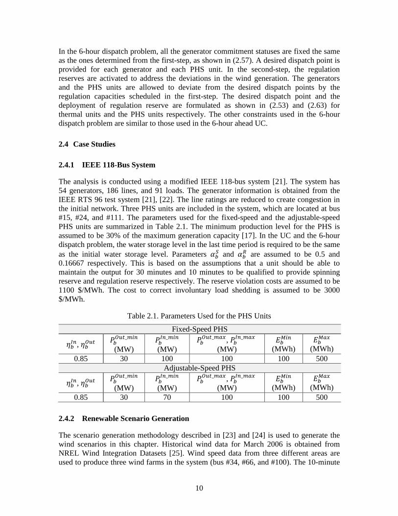
10

In the 6-hour dispatch problem, all the generator commitment statuses are fixed the same as the ones determined from the first-step, as shown in (2.57). A desired dispatch point is provided for each generator and each PHS unit. In the second-step, the regulation reserves are activated to address the deviations in the wind generation. The generators and the PHS units are allowed to deviate from the desired dispatch points by the regulation capacities scheduled in the first-step. The desired dispatch point and the deployment of regulation reserve are formulated as shown in (2.53) and (2.63) for thermal units and the PHS units respectively. The other constraints used in the 6-hour dispatch problem are similar to those used in the 6-hour ahead UC.

2.4 Case Studies

2.4.1 IEEE 118-Bus System

The analysis is conducted using a modified IEEE 118-bus system [21]. The system has 54 generators, 186 lines, and 91 loads. The generator information is obtained from the IEEE RTS 96 test system [21], [22]. The line ratings are reduced to create congestion in the initial network. Three PHS units are included in the system, which are located at bus #15, #24, and #111. The parameters used for the fixed-speed and the adjustable-speed PHS units are summarized in Table 2.1. The minimum production level for the PHS is assumed to be 30% of the maximum generation capacity [17]. In the UC and the 6-hour dispatch problem, the water storage level in the last time period is required to be the same as the initial water storage level. Parameters 𝛼𝑏𝑆 and 𝛼𝑏𝑅 are assumed to be 0.5 and 0.16667 respectively. This is based on the assumptions that a unit should be able to maintain the output for 30 minutes and 10 minutes to be qualified to provide spinning reserve and regulation reserve respectively. The reserve violation costs are assumed to be 1100 $/MWh. The cost to correct involuntary load shedding is assumed to be 3000 $/MWh.

Table 2.1. Parameters Used for the PHS Units

Fixed-Speed PHS

𝜂𝑏𝐼𝑠, 𝜂𝑏𝑂𝑢𝑖 𝑃𝑏𝑂𝑢𝑖_𝑠𝑖𝑠 (MW)

𝑃𝑏𝐼𝑠_𝑠𝑖𝑠

(MW) 𝑃𝑏𝑂𝑢𝑖_𝑠𝑠𝑠, 𝑃𝑏

𝐼𝑠_𝑠𝑠𝑠 (MW)

𝐸𝑏𝑀𝑖𝑠 (MWh)

𝐸𝑏𝑀𝑠𝑠 (MWh)

0.85 30 100 100 100 500 Adjustable-Speed PHS

𝜂𝑏𝐼𝑠, 𝜂𝑏𝑂𝑢𝑖 𝑃𝑏𝑂𝑢𝑖_𝑠𝑖𝑠 (MW)

𝑃𝑏𝐼𝑠_𝑠𝑖𝑠

(MW) 𝑃𝑏𝑂𝑢𝑖_𝑠𝑠𝑠, 𝑃𝑏

𝐼𝑠_𝑠𝑠𝑠 (MW)

𝐸𝑏𝑀𝑖𝑠 (MWh)

𝐸𝑏𝑀𝑠𝑠 (MWh)

0.85 30 70 100 100 500

2.4.2 Renewable Scenario Generation

The scenario generation methodology described in [23] and [24] is used to generate the wind scenarios in this chapter. Historical wind data for March 2006 is obtained from NREL Wind Integration Datasets [25]. Wind speed data from three different areas are used to produce three wind farms in the system (bus #34, #66, and #100). The 10-minute

11

autoregressive integrated moving average (ARIMA) models are used to fit the wind speed data and produce the time series models for each wind farm location. The wind scenarios are then generated for each location using the obtained time series models and an estimate of the aggregate power curves. The generated wind scenarios are normalized with the average such that the resulted forecast error is about 5% to 8%. The mean value of the time series is used in the 6-hour ahead UC as the actual wind forecast.

Using the approach described above, 150 wind scenarios are generated. The case study is conducted for 20% wind penetration level. The wind penetration level is defined as the ratio of total daily wind generation to the total daily demand.

2.4.3 Simulation Setup

The simulation is conducted as follows. Wind scenarios are generated using the approach described in the previous subsection. The 6-hour ahead UC is solved in the first-step using the load and wind data for the first six hours in a day. After the UC is solved, the UC solution is tested against 150 wind scenarios in the second-step to see if the scheduled reserves are able to balance the uncertainty in wind generation. The above process is repeated two times with the fixed-speed PHS and the adjustable-speed PHS in the system respectively. Metrics are reported to evaluate and compare the effectiveness of the fixed-speed PHS and the adjustable-speed PHS in providing regulation reserves.

2.4.4 The First-Step and the 6-Hour Ahead Unit Commitment

In the first-step, the UC is solved with the fixed-speed and the adjustable-speed PHS units in the system respectively. In Table 2.2, the total system cost, involuntary load shedding, wind curtailment and reserve violations are reported for the 6-hour ahead UC. The reserve violations in Table 2.2 represent the sum of all the violations in reserve requirements in the system. In Table 2.3, the average regulation reserve capacity scheduled for the fixed-speed PHS and the adjustable-speed PHS in each time period is presented. The average regulation reserve capacity is calculated as

AURRC = ∑ ∑ 𝑟𝑏𝑡𝑅+

𝑏𝑡𝑁𝑇

(2.71)

ADRRC = ∑ ∑ 𝑟𝑏𝑡𝑅−

𝑏𝑡𝑁𝑇

(2.72)

where AURRC (ADRRC) represents the mean value of the up (down) regulation reserve capacities scheduled for the PHS units in each time period. The parameter 𝑁𝑇 represents the number of time periods included in the 6-hour ahead UC problem. In Table 2.3, the first and the second columns present the average up and down regulation reserve capacities scheduled for the PHS units, while the third and the fourth column show the scheduled regulation reserve capacities for the PHS units in the pumping mode.

As shown in Table 2.2, the total system costs are very close for the cases with the fixed-speed and the adjustable-speed PHS. This is because only the capacities of the reserves are scheduled in the first-step. From Table 2.3, it can be seen that more up regulation

12

reserves are scheduled for the fixed-speed PHS and the adjustable-speed PHS has more down regulation reserves scheduled in each time period. For the adjustable-speed PHS, in average 2.9 MW of up regulation reserves are scheduled in the pumping mode in each time period, which accounts for about 50% of the total up regulation reserves scheduled for the adjustable-speed PHS. For the fixed-speed PHS, since the input power cannot be adjusted during the pumping process, no regulation reserves are scheduled for the fixed-speed PHS while in pumping mode. Since only the reserve capacities are determined in the first-step, the performance of the two PHS technologies is not fully assessed.

Table 2.2. System Results for the 6-Hour Ahead Unit Commitment

PHS Type Total System Cost ($)

Involuntary Load Shedding

(MWh)

Wind Curtailment

(MWh)

Reserve Violations

(MWh) Fixed-Speed 397885 0 4 0

Adjustable-Speed 397848 0 0 0

Table 2.3. Average Regulation Reserve Capacities Scheduled for the Fixed-Speed and the Adjustable-Speed PHS in Each Time Period

PHS Type Average 𝑟𝑏𝑖𝑅+ (MW)

Average 𝑟𝑏𝑖𝑅− (MW)

𝑟𝑏𝑖𝑅+ Provided in the Pumping Mode (MW)

𝑟𝑏𝑖𝑅− Provided in the Pumping Mode (MW)

Fixed-Speed 8.0 8.0 0 0 Adjustable-Speed 5.7 35.5 2.9 0

2.4.5 The Second-Step and the 6-Hour Dispatch

In the second-step, the 6-hour dispatch problem is solved to simulate the activation of the regulation reserves. The expected total system cost, expected involuntary load shedding, expected wind curtailment, and expected reserve violations are reported in Table 2.4 for the cases with the fixed-speed and the adjustable-speed PHS respectively. As shown in Table 2.4, the cases with the adjustable-speed PHS have less involuntary load shedding and lower total system cost compared to the case with the fixed-speed PHS. The relative cost saving by using the adjustable-speed PHS is about $8127, or 1.9% compared to the cases with the fixed-speed PHS.

In Table 2.5, the regulation reserves provided by the PHS in the second-step are presented. The result in Table 2.5 represents the expected value of sum of the regulation reserves provided by all the PHS units in the system across six hours. It can be noted from Table 2.5 that both the up and down regulation reserves provided by the adjustable-speed PHS are higher than the ones provided by the fixed-speed PHS. For adjustable-speed PHS, 6.8 MWh of regulation reserves are provided in the pumping mode, which accounts for about 72% of the total up regulation reserves it provides. This result indicates that the capability of the adjustable-speed PHS to provide regulation reserves is

13

significantly enhanced by being able to vary the input power in the pumping mode. The result in the second-step demonstrates that the adjustable-speed PHS is more flexible and effective in providing regulation reserves in systems with renewable resources than the traditional fixed-speed PHS.

Table 2.4. Expected System Results for the 6-hour Dispatch Problem

PHS Type Total System Cost ($)

Involuntary Load Shedding (MWh)

Wind Curtailment

(MWh)

Reserve Violations

(MWh) Fixed-Speed 427849 9 16 0

Adjustable-Speed 419722 7 23 0

Table 2.5. Expected Total Regulation Reserves Provided by the Fixed-Speed and Adjustable-Speed PHS in the 6-Hour Dispatch Problem

PHS Type Total 𝑟𝑏𝑖𝑅+ (MWh)

Total 𝑟𝑏𝑖𝑅− (MWh)

𝑟𝑏𝑖𝑅+ Provided in Pumping Mode

(MWh)

𝑟𝑏𝑖𝑅− Provided in Pumping Mode

(MWh) Fixed-Speed 1.3 1.3 0 0

Adjustable-Speed 9.4 7.6 6.8 0

A statistical description of the total system cost in the second-step is presented in Table 2.6. From Table 2.6, it can be noted that for the cases with the adjustable-speed PHS, the standard deviation is reduced compared with the cases with the fixed-speed PHS. The minimum values are close for the cases with the fixed-speed and the adjustable-speed PHS. However, the maximum value is lower for the cases with the adjustable-speed PHS. The result in Table 2.6 demonstrates that the adjustable-speed PHS is more effective in managing the uncertainties in renewable resources than the fixed-speed PHS.

Table 2.6. Statistical Description of the Total System Cost in the 6-Hour Dispatch Problem ($)

Fixed-Speed Adjustable-Speed

Mean 427849 419722 Median 413485 411330

Standard Deviation 38127 26490 Minimum 397470 397720 Maximum 571878 516949

2.5 Conclusion

Pumped hydro storage has been considered as an attractive storage solution to facilitate the integration of high levels of renewable resources. Two PHS technologies are introduced and compared in this chapter, namely the fixed-speed and the adjustable-speed

14

PHS. The mathematical models are developed for the two PHS technologies. A two-step approach is proposed to evaluate the performance of the fixed-speed and the adjustable-speed PHS in systems with renewable resources. In the first-step, the scheduling costs and the scheduled regulation reserve capacities are compared for the cases with the fixed-speed and the adjustable-speed PHS. The result shows that for the adjustable-speed PHS, a substantial proportion of regulation reserves are scheduled in the pumping mode. In the second-step, a 6-hour dispatch problem is formulated to simulate the activation of the regulation reserves. It is shown in the second-step that by using the adjustable-speed PHS, the total system costs and the involuntary load shedding are reduced. The regulation reserve provided by the adjustable-speed PHS is much larger than that provided by the fixed-speed PHS. For the adjustable-speed PHS, about 72% of its regulation reserves are provided in the pumping mode. This result demonstrates that by having the capability to vary the input power in the pumping mode, the adjustable-speed PHS is more effective than the fixed-speed PHS in balancing renewable uncertainties in the system.

15

3. Enhanced Utilization of Pumped Hydro Storage in Power System Operation using Policy Functions

Despite the growing interests in energy storage, the existing energy and market management systems do not make full use of the flexibility of the PHS. In this chapter, a policy function based approach is proposed to enhance the utilization of the PHS with minimal added computational difficulty. The study is focused on the real-time operation of the PHS. The performance of the approach is evaluated and compared with other benchmark approaches using the IEEE RTS 24-bus system.

3.1 Introduction

Driven by the rapid integration of high levels of renewable energy, power system has experienced an increasing need for flexible generation resources. As energy storage technologies have the capability to shift energy across hours and follow fast-ramping signal, it provides an attractive solution to facilitate high levels of renewable resources in power systems. In California, an energy storage mandate has been adopted to require the utility companies to install 1325 MW of energy storage by 2020 [26]. As renewable penetration level increases, energy storage is expected to be more valuable to the grid. As the most commercially matured large-scale energy storage technology, the PHS has been widely used around the world. With the fast expansion of renewable generation, new interests have been focused on using the PHS to facilitate the integration of high levels of renewable resources [11]-[14].

While there are growing interests in energy storage in recent years, the existing energy and market management systems do not adequately account for the characteristics of energy storage. Today, a typical way to operate the PHS is to provide an operational schedule based on a prior look-ahead planning stage. As the real-time model has a limited look-ahead timeframe and the operators wish to ensure the PHS has the expected capability in future time periods, the consumption and production of the PHS are fixed during real-time operation, or left with limited room for adjustments. However, as renewable penetration increases, the uncertainties introduced by renewable resources may reduce the effectiveness of such operation approach. By using such a look-ahead planning strategy, the flexibility of the PHS cannot be fully utilized.

In this chapter, the challenges associated with utilizing the PHS in real-time operation with renewable resources are addressed. For storage technologies, the consumption and production capabilities are constrained by their storage levels. As real-time operation has limited look-ahead functionalities, a decision made for the current time period may potentially influence the consumption and production capabilities in future time periods. Therefore, a decision tool is needed to optimally operate the PHS across multiple time periods. The decision tool should be able to make optimal decisions for energy storage in current time period while taking into account future uncertainties. In this chapter, a policy function based approach is proposed to enhance the utilization of the PHS in real-time operation. The policy function based approach is able to address the challenges with uncertainty and limited look-ahead functionality in real-time operation, while having

16

minimal added computational difficulty to the existing energy and market management systems.

3.2 Policy Functions and the Proposed Framework

A policy function is a rule that describes the control action as a function of the state [28]. In power systems, the application of policy functions is not new, such as the use of reserve policies. For example, contingency reserve (quantity) requirement is one kind of reserve policies that is used to ensure the N-1 reliability of the system. However, such contingency reserve requirement only functions as an approximation to the N-1 reliability criterion, since the reserves may not be delivered due to transmission congestions. While stochastic programming models can explicitly formulate the N-1 reliability and implicitly determine both the quantity and location of the reserves, such models are not computational tractable for large-scale power systems. In order to improve the deliverability of reserves with tractable computational complexity, reserve zones are used along with reserve requirements to construct an enhanced reserve policy. The use of reserve requirement and reserve zone can be recognized as a strategy to approximate the function of stochastic programming models while keeping the computational complexity scalable for large-scale power systems.

Following the similar philosophy behind reserve policies, a policy function based approach is developed in this chapter. As policy functions have different forms, the one implemented in this chapter is referred to as the policy function approximation (PFA). For a given state, a PFA returns an action without using the information of future forecast or resorting to any form of imbedded optimization [29]. Different from stochastic programming models, which determine a decision by explicitly considering multiple future realizations, a PFA returns an action for a given state based on the knowledge extracted from prior state and action pairs. Therefore, by using the PFA based approach, computational burden is shifted from real-time to offline-study stages. The proposed PFA is to be utilized along with deterministic models to achieve what could be otherwise accomplished by stochastic programing models, but with tractable computation complexity. While the policy function is primarily developed for the operation of the PHS, the same design philosophy could be generalized to other power system applications.

An overview of the PFA based approach is illustrated in Fig. 3.1. The proposed approach consists of three phases. The first phase is the derivation of the PFAs. In the first phase, a Monte-Carlo based simulation, which is referred to as the stochastic simulation, is performed to obtain optimal schedules for the PHS with possible realizations of the wind generation next day. The data obtained from the stochastic simulation is then used to derive the PFAs. The generation of PFAs is carried out prior to the actual operating stage. It can be conducted as an offline analysis which utilizes historical wind data, or as a day-ahead analysis that relies on day-ahead wind forecasts. The second phase is the selection of the PFAs. This phase is implemented between the day-ahead market (DAM) and the real-time market (RTM). In the second phase, updated wind forecasts are obtained and the derived PFAs are tested against the updated wind forecasts. The policy function that has the best performance is selected. In the third phase, the PFA selected in the second

17

phase is implemented in the real-time market to improve the operational scheme of the PHS.

Enhanced Real-time Market

Day-ahead Market

Test and Choose the Best Policy Function to Use

Monte-Carlo Simulation to Obtain Optimal PHS Schedules

Obtain Policy Functions for PHS

Generate Scenarios

Wind Forecast

1

23

Adjustment teriod after Day-ahead Market

Derive tolicy Cunctions (hffline or Day-ahead Analysis )

Fig. 3.1. Overview of the proposed approach

3.3 Simulation Setup

In this work, the proposed PFA is generated using the day-ahead wind forecasts. A flowchart describing the simulation process is presented in Fig. 3.2. Wind scenarios are first generated and the day-ahead UC is solved. Once the commitment schedule is obtained, stochastic simulation is performed to determine the optimal schedules for the PHS with different wind scenarios. The data obtained from the stochastic simulation is used to generate the PFA. After the PFA is obtained, the performance of the derived PFA is evaluated and compared with other benchmark approaches. The mathematical models involved in the simulation process are described in the following subsections.

18

Generate Renewable Scenarios based on Forecast

Solve Day-Ahead Deterministic Unit Commitment

Perform Stochastic Simulation

Obtain Policy Functions for the PHS

Test Policy Function and Compare with Benchmark Methods

Fig. 3.2. Flowchart for the simulation process

3.4 Day-Ahead Unit Commitment

The day-ahead UC model is formulated as a mixed integer linear program (MILP). It is assumed that the PHS unit is a system asset. The formulation of the UC model is shown in (3.1)-(3.28), where the objective (3.1) is to minimize total system operating costs and violation costs. The violation costs include the costs of involuntary load shedding and the costs of not meeting the reserve requirements. Constraint (3.2) guarantees the power balance at every bus. Constraint (3.3) represents the dc power flow on each line and (3.4) is the line-flow limit constraint. Limits on the power output for each generator are presented in (3.5) and (3.6). The minimum up and down time constraints are shown in (3.7)-(3.9). Constraints (3.10)-(3.12) represent the ramp rates for regulation, spinning and non-spinning reserves for the thermal units. The hourly ramp rate constraints are shown in (3.13) and (3.14). The model for the PHS is shown in constraints (3.15)-(3.23). The PHS included in the study is assumed to be an adjustable-speed PHS. Constraints (3.15)-(3.18) represent the limits on regulation and spinning reserves provided by the PHS. Constraint (3.19) is the energy balance constraint. The limits on consumption and production for the PHS are presented in (3.20) and (3.21). Constraint (3.22) requires that the PHS can only be in one mode at one time period. Constraint (3.23) formulates the limits on the water reservoir of the PHS. The system-wide regulation and spinning reserve requirements constraints are presented in (3.24)-(3.28). The regulation reserve requirement is set to be 2% of the hourly load. The operating reserve (sum of spinning and non-spinning reserves) is required to be greater or equal to the single largest generator contingency plus the NREL’s “3+5” reserve rule [18]. The NREL’s “3+5” reserve rule is used to address the uncertainty in renewable resources. The reserve requirements can be violated for a predetermined penalty price.

Minimize:

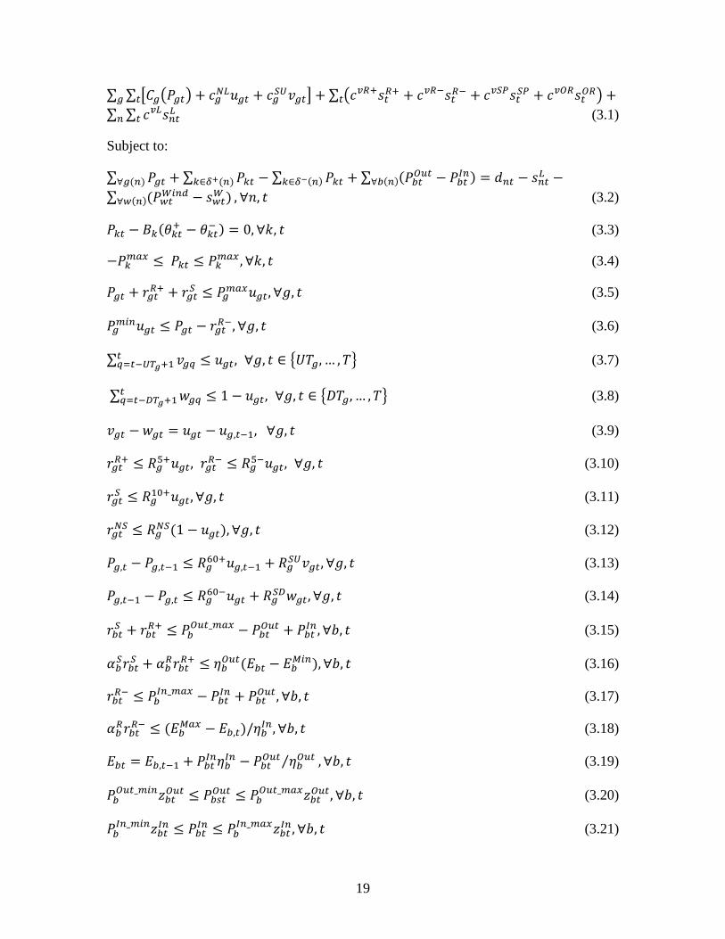
19

∑ ∑ �𝐶𝑔�𝑃𝑔𝑖� + 𝑐𝑔𝑁𝐿𝑢𝑔𝑖 + 𝑐𝑔𝑆𝑆𝑣𝑔𝑖�𝑖𝑔 + ∑ �𝑐𝑣𝑅+𝑠𝑖𝑅+ + 𝑐𝑣𝑅−𝑠𝑖𝑅− + 𝑐𝑣𝑆𝑃𝑠𝑖𝑆𝑃 + 𝑐𝑣𝑂𝑅𝑠𝑖𝑂𝑅�𝑖 +∑ ∑ 𝑐𝑣𝐿𝑠𝑠𝑖𝐿𝑖𝑠 (3.1)

Subject to:

∑ 𝑃𝑔𝑖∀𝑔(𝑠) + ∑ 𝑃𝑘𝑖𝑘∈𝛿+(𝑠) − ∑ 𝑃𝑘𝑖𝑘∈𝛿−(𝑠) + ∑ (𝑃𝑏𝑖𝑂𝑢𝑖 − 𝑃𝑏𝑖𝐼𝑠)∀𝑏(𝑠) = 𝑑𝑠𝑖 − 𝑠𝑠𝑖𝐿 −∑ (𝑃𝐿𝑖𝑊𝑖𝑠𝑑 − 𝑠𝐿𝑖𝑊 )∀𝐿(𝑠) ,∀𝑚, 𝑅 (3.2)

𝑃𝑘𝑖 − 𝐵𝑘(𝜃𝑘𝑖+ − 𝜃𝑘𝑖− ) = 0,∀𝑘, 𝑅 (3.3)

−𝑃𝑘𝑠𝑠𝑠 ≤ 𝑃𝑘𝑖 ≤ 𝑃𝑘𝑠𝑠𝑠 ,∀𝑘, 𝑅 (3.4)

𝑃𝑔𝑖 + 𝑟𝑔𝑖𝑅+ + 𝑟𝑔𝑖𝑆 ≤ 𝑃𝑔𝑠𝑠𝑠𝑢𝑔𝑖,∀𝑔, 𝑅 (3.5)

𝑃𝑔𝑠𝑖𝑠𝑢𝑔𝑖 ≤ 𝑃𝑔𝑖 − 𝑟𝑔𝑖𝑅−,∀𝑔, 𝑅 (3.6)

∑ 𝑣𝑔𝑔𝑖𝑔=𝑖−𝑆𝑇𝑔+1 ≤ 𝑢𝑔𝑖, ∀𝑔, 𝑅 ∈ �𝑈𝐷𝑔, … ,𝐷� (3.7)

∑ 𝑤𝑔𝑔𝑖𝑔=𝑖−𝑔𝑇𝑔+1 ≤ 1 − 𝑢𝑔𝑖, ∀𝑔, 𝑅 ∈ �𝐷𝐷𝑔, … ,𝐷� (3.8)

𝑣𝑔𝑖 − 𝑤𝑔𝑖 = 𝑢𝑔𝑖 − 𝑢𝑔,𝑖−1, ∀𝑔, 𝑅 (3.9)

𝑟𝑔𝑖𝑅+ ≤ 𝑅𝑔5+𝑢𝑔𝑖, 𝑟𝑔𝑖𝑅− ≤ 𝑅𝑔5−𝑢𝑔𝑖, ∀𝑔, 𝑅 (3.10)

𝑟𝑔𝑖𝑆 ≤ 𝑅𝑔10+𝑢𝑔𝑖,∀𝑔, 𝑅 (3.11)

𝑟𝑔𝑖𝑁𝑆 ≤ 𝑅𝑔𝑁𝑆(1 − 𝑢𝑔𝑖),∀𝑔, 𝑅 (3.12)

𝑃𝑔,𝑖 − 𝑃𝑔,𝑖−1 ≤ 𝑅𝑔60+𝑢𝑔,𝑖−1 + 𝑅𝑔𝑆𝑆𝑣𝑔𝑖,∀𝑔, 𝑅 (3.13)

𝑃𝑔,𝑖−1 − 𝑃𝑔,𝑖 ≤ 𝑅𝑔60−𝑢𝑔𝑖 + 𝑅𝑔𝑆𝑔𝑤𝑔𝑖,∀𝑔, 𝑅 (3.14)

𝑟𝑏𝑖𝑆 + 𝑟𝑏𝑖𝑅+ ≤ 𝑃𝑏𝑂𝑢𝑖_𝑠𝑠𝑠 − 𝑃𝑏𝑖𝑂𝑢𝑖 + 𝑃𝑏𝑖𝐼𝑠,∀𝑏, 𝑅 (3.15)

𝛼𝑏𝑆𝑟𝑏𝑖𝑆 + 𝛼𝑏𝑅𝑟𝑏𝑖𝑅+ ≤ 𝜂𝑏𝑂𝑢𝑖(𝐸𝑏𝑖 − 𝐸𝑏𝑀𝑖𝑠),∀𝑏, 𝑅 (3.16)

𝑟𝑏𝑖𝑅− ≤ 𝑃𝑏𝐼𝑠_𝑠𝑠𝑠 − 𝑃𝑏𝑖𝐼𝑠 + 𝑃𝑏𝑖𝑂𝑢𝑖,∀𝑏, 𝑅 (3.17)

𝛼𝑏𝑅𝑟𝑏𝑖𝑅− ≤ (𝐸𝑏𝑀𝑠𝑠 − 𝐸𝑏,𝑖)/𝜂𝑏𝐼𝑠,∀𝑏, 𝑅 (3.18)

𝐸𝑏𝑖 = 𝐸𝑏,𝑖−1 + 𝑃𝑏𝑖𝐼𝑠𝜂𝑏𝐼𝑠 − 𝑃𝑏𝑖𝑂𝑢𝑖 𝜂𝑏𝑂𝑢𝑖⁄ ,∀𝑏, 𝑅 (3.19)

𝑃𝑏𝑂𝑢𝑖_𝑠𝑖𝑠𝑧𝑏𝑖𝑂𝑢𝑖 ≤ 𝑃𝑏𝑠𝑖𝑂𝑢𝑖 ≤ 𝑃𝑏

𝑂𝑢𝑖_𝑠𝑠𝑠𝑧𝑏𝑖𝑂𝑢𝑖,∀𝑏, 𝑅 (3.20)

𝑃𝑏𝐼𝑠_𝑠𝑖𝑠𝑧𝑏𝑖𝐼𝑠 ≤ 𝑃𝑏𝑖𝐼𝑠 ≤ 𝑃𝑏

𝐼𝑠_𝑠𝑠𝑠𝑧𝑏𝑖𝐼𝑠,∀𝑏, 𝑅 (3.21)

20

𝑧𝑏𝑖𝑂𝑢𝑖 + 𝑧𝑏𝑖𝐼𝑠 ≤ 1,∀𝑏, 𝑅 (3.22)

𝐸𝑏𝑀𝑖𝑠 ≤ 𝐸𝑏𝑖 ≤ 𝐸𝑏𝑀𝑠𝑠,∀𝑏, 𝑅 (3.23)

∑ 𝑟𝑔𝑖𝑅+𝑔 + ∑ 𝑟𝑏𝑖𝑅+𝑏 ≥ 0.02∑ 𝑑𝑠𝑖𝑠 − 𝑠𝑖𝑅+,∀𝑅 (3.24)

∑ 𝑟𝑔𝑖𝑅−𝑔 + ∑ 𝑟𝑏𝑖𝑅−𝑏 ≥ 0.02∑ 𝑑𝑠𝑖𝑠 − 𝑠𝑖𝑅−,∀𝑅 (3.25)

𝑄𝑖𝑂𝑅 ≥ 𝑃𝑔𝑖 + 𝑟𝑔𝑖𝑆 + 0.03∑ 𝑑𝑠𝑖𝑠 + 0.05∑ 𝑃𝐿𝑖𝑊𝑖𝑠𝑑𝐿 ,∀𝑔, 𝑅 (3.26)

∑ 𝑟𝑔𝑖𝑆𝑔 + ∑ 𝑟𝑏𝑖𝑆𝑏 + ∑ 𝑟𝑔𝑖𝑁𝑆𝑔 ≥ 𝑄𝑖𝑂𝑅 − 𝑠𝑖𝑂𝑅 ,∀𝑅 (3.27)

∑ 𝑟𝑔𝑖𝑆𝑔 + ∑ 𝑟𝑏𝑖𝑆𝑏 ≥ 0.5𝑄𝑖𝑂𝑅 − 𝑠𝑖𝑆𝑃,∀𝑅 (3.28)

3.5 Stochastic Simulation and the 24-Hour Dispatch Model

After the day-ahead UC is solved, the stochastic simulation is performed to obtain the optimal schedules of the PHS with different wind scenarios. In the stochastic simulation, each wind scenario is solved using a 24-hour dispatch model. In the 24-hour dispatch model, the 24 time periods are solved together in one optimization program. The primary function of the stochastic simulation is to obtain PHS schedules with different wind scenarios assuming that the entire path of the wind scenario is known. After the stochastic simulation is performed, an optimal PHS schedule is determined for each wind scenario. The obtained PHS schedules are then used to generate the PFA that returns an action for the given operating conditions.

The formulation of the 24-hour dispatch model is presented in (3.29)-(3.53). The commitment status for slow units is fixed the same as the ones from day-ahead solution, as shown in (3.33). Also, as shown in (3.35), a desired dispatch point is provided for each slow unit and the slow units can deviate from the desired dispatch point within the 10-minute ramp rate. In the 24-hour dispatch problem, only the generator contingency reserve requirement is modeled (3.40). The other constraints used in the 24-hour dispatch model are similar to those used in the day-ahead UC model.

Minimize:

∑ ∑ �𝐶𝑔�𝑃𝑔𝑖� + 𝑐𝑔𝑁𝐿𝑢𝑔𝑖 + 𝑐𝑔𝑆𝑆𝑣𝑔𝑖�𝑖𝑔 + ∑ ∑ 𝑐𝑣𝐿𝑠𝑠𝑖𝐿𝑖𝑠 + ∑ �𝑐𝑣𝑅+𝑠𝑖𝑅+ + 𝑐𝑣𝑅−𝑠𝑖𝑅− +𝑖𝑐𝑣𝑆𝑃𝑠𝑖𝑆𝑃 + 𝑐𝑣𝑂𝑅𝑠𝑖𝑂𝑅� (3.29)

Subject to:

∑ 𝑃𝑔𝑖∀𝑔(𝑠) + ∑ 𝑃𝑘𝑖𝑘∈𝛿+(𝑠) − ∑ 𝑃𝑘𝑖𝑘∈𝛿−(𝑠) + ∑ (𝑃𝑏𝑖𝑂𝑢𝑖 − 𝑃𝑏𝑖𝐼𝑠)∀𝑏(𝑠) = 𝑑𝑠𝑖 − 𝑠𝑠𝑖𝐿 −∑ (𝑃𝐿𝑖𝑊𝑖𝑠𝑑 − 𝑠𝐿𝑖𝑊 )∀𝐿(𝑠) ,∀𝑚, 𝑅 (3.30)

𝑃𝑘𝑖 − 𝐵𝑘(𝜃𝑘𝑖+ − 𝜃𝑘𝑖− ) = 0,∀𝑘, 𝑅 (3.31)

−𝑃𝑘𝑠𝑠𝑠 ≤ 𝑃𝑘𝑖 ≤ 𝑃𝑘𝑠𝑠𝑠 ,∀𝑘, 𝑅 (3.32)

21

𝑢𝑔𝑖 = 𝑢𝑔𝑖 , 𝑣𝑔𝑖 = 𝑣𝑔𝑖,𝑤𝑔𝑖 = 𝑤𝑔𝑖,∀𝑔 ∈ Ω𝐺𝑠, 𝑅 (3.33)

𝑃𝑔𝑠𝑖𝑠𝑢𝑔𝑖 + 𝑟𝑔𝑖𝑅− ≤ 𝑃𝑔𝑖 ≤ 𝑃𝑔𝑠𝑠𝑠𝑢𝑔𝑖 − 𝑟𝑔𝑖𝑅+ − 𝑟𝑔𝑖𝑆 ,∀𝑔, 𝑅 (3.34)

(𝑃�𝑔𝑖 − 𝑅𝑔10−)𝑢𝑔𝑖 ≤ 𝑃𝑔𝑖 ≤ (𝑃�𝑔𝑖 + 𝑅𝑔10+)𝑢𝑔𝑖,∀𝑔 ∈ 𝛺𝐺𝑠 , 𝑅 (3.35)

𝑃𝑔,𝑖 − 𝑃𝑔,𝑖−1 ≤ 𝑅𝑔60+𝑢𝑔,𝑖−1 + 𝑅𝑔𝑆𝑆𝑣𝑔𝑖,∀𝑔, 𝑅 (3.36)

𝑃𝑔,𝑖−1 − 𝑃𝑔,𝑖 ≤ 𝑅𝑔60−𝑢𝑔𝑖 + 𝑅𝑔𝑆𝑔𝑤𝑔𝑖,∀𝑔, 𝑅 (3.37)

𝑟𝑔𝑖𝑅+ ≤ 𝑅𝑔5+𝑢𝑔𝑖, 𝑟𝑔𝑖𝑅− ≤ 𝑅𝑔5−𝑢𝑔𝑖,∀𝑔, 𝑅 (3.38)

𝑟𝑔𝑖𝑆 ≤ 𝑅𝑔10+𝑢𝑔𝑖,∀𝑔, 𝑅 (3.39)

𝑄𝑖𝑂𝑅 ≥ 𝑃𝑔𝑖 + 𝑟𝑔𝑖𝑆 ,∀𝑔, 𝑅 (3.40)

∑ 𝑟𝑔𝑖𝑅+𝑔 + ∑ 𝑟𝑏𝑖𝑅+𝑏 ≥ 𝑄𝑖𝑅+ − 𝑠𝑖𝑅+,∀𝑅 (3.41)

∑ 𝑟𝑔𝑖𝑅−𝑔 + ∑ 𝑟𝑏𝑖𝑅−𝑏 ≥ 𝑄𝑖𝑅− − 𝑠𝑖𝑅−,∀𝑅 (3.42)

∑ 𝑟𝑔𝑖𝑆𝑔 + ∑ 𝑟𝑏𝑖𝑆𝑏 ≥ 0.5𝑄𝑖𝑂𝑅 − 𝑠𝑖𝑆𝑃,∀𝑅 (3.43)

∑ 𝑟𝑔𝑖𝑆𝑔 + ∑ 𝑟𝑏𝑖𝑆𝑏 + ∑ 𝑟𝑔𝑖𝑁𝑆𝑔 ≥ 𝑄𝑖𝑂𝑅 − 𝑠𝑖𝑂𝑅 ,∀𝑔, 𝑅 (3.44)

𝑟𝑏𝑆 + 𝑟𝑏𝑖𝑅+ ≤ 𝑃𝑏𝑂𝑢𝑖_𝑠𝑠𝑠 − 𝑃𝑏𝑖𝑂𝑢𝑖 + 𝑃𝑏𝑖𝐼𝑠,∀𝑏, 𝑅 (3.45)

𝛽𝑏𝑆𝑟𝑏𝑖𝑆 + 𝛽𝑏𝑅𝑟𝑏𝑖𝑅+ ≤ 𝜂𝑏𝑂𝑢𝑖(𝐸𝑏𝑖 − 𝐸𝑏𝑀𝑖𝑠),∀𝑏, 𝑅 (3.46)

𝑟𝑏𝑅− ≤ 𝑃𝑏𝐼𝑠_𝑠𝑠𝑠 − 𝑃𝑏𝑖𝐼𝑠 + 𝑃𝑏𝑖𝑂𝑢𝑖,∀𝑏, 𝑅 (3.47)

𝛽𝑏𝑅𝑟𝑏𝑖𝑅− ≤ (𝐸𝑏𝑀𝑠𝑠 − 𝐸𝑏𝑖)/𝜂𝑏𝐼𝑠,∀𝑏, 𝑅 (3.48)

𝐸𝑏𝑖 = 𝐸𝑏,𝑖−1 + 𝑃𝑏𝑖𝐼𝑠𝜂𝑏𝐼𝑠 − 𝑃𝑏𝑖𝑂𝑢𝑖 𝜂𝑏𝑂𝑢𝑖⁄ ,∀𝑏, 𝑅 (3.49)

𝑃𝑏𝑂𝑢𝑖_𝑠𝑖𝑠𝑧𝑏𝑖𝑂𝑢𝑖 ≤ 𝑃𝑏𝑖𝑂𝑢𝑖 ≤ 𝑃𝑏

𝑂𝑢𝑖_𝑠𝑠𝑠𝑧𝑏𝑖𝑂𝑢𝑖,∀𝑏, 𝑅 (3.50)

𝑃𝑏𝐼𝑠_𝑠𝑖𝑠𝑧𝑏𝑖𝐼𝑠 ≤ 𝑃𝑏𝑖𝐼𝑠 ≤ 𝑃𝑏

𝐼𝑠_𝑠𝑠𝑠𝑧𝑏𝑖𝐼𝑠,∀𝑏, 𝑅 (3.51)

𝑧𝑏𝑖𝑂𝑢𝑖 + 𝑧𝑏𝑖𝐼𝑠 ≤ 1,∀𝑏, 𝑅 (3.52)

𝐸𝑏𝑀𝑖𝑠 ≤ 𝐸𝑏𝑖 ≤ 𝐸𝑏𝑀𝑠𝑠,∀𝑏, 𝑅 (3.53)

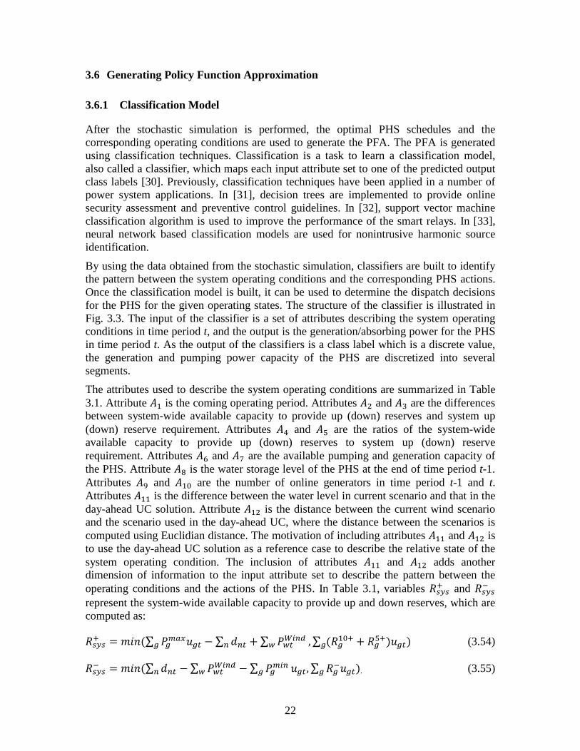
22

3.6 Generating Policy Function Approximation

3.6.1 Classification Model

After the stochastic simulation is performed, the optimal PHS schedules and the corresponding operating conditions are used to generate the PFA. The PFA is generated using classification techniques. Classification is a task to learn a classification model, also called a classifier, which maps each input attribute set to one of the predicted output class labels [30]. Previously, classification techniques have been applied in a number of power system applications. In [31], decision trees are implemented to provide online security assessment and preventive control guidelines. In [32], support vector machine classification algorithm is used to improve the performance of the smart relays. In [33], neural network based classification models are used for nonintrusive harmonic source identification.

By using the data obtained from the stochastic simulation, classifiers are built to identify the pattern between the system operating conditions and the corresponding PHS actions. Once the classification model is built, it can be used to determine the dispatch decisions for the PHS for the given operating states. The structure of the classifier is illustrated in Fig. 3.3. The input of the classifier is a set of attributes describing the system operating conditions in time period t, and the output is the generation/absorbing power for the PHS in time period t. As the output of the classifiers is a class label which is a discrete value, the generation and pumping power capacity of the PHS are discretized into several segments.

The attributes used to describe the system operating conditions are summarized in Table 3.1. Attribute 𝐴1 is the coming operating period. Attributes 𝐴2 and 𝐴3 are the differences between system-wide available capacity to provide up (down) reserves and system up (down) reserve requirement. Attributes 𝐴4 and 𝐴5 are the ratios of the system-wide available capacity to provide up (down) reserves to system up (down) reserve requirement. Attributes 𝐴6 and 𝐴7 are the available pumping and generation capacity of the PHS. Attribute 𝐴8 is the water storage level of the PHS at the end of time period t-1. Attributes 𝐴9 and 𝐴10 are the number of online generators in time period t-1 and t. Attributes 𝐴11 is the difference between the water level in current scenario and that in the day-ahead UC solution. Attribute 𝐴12 is the distance between the current wind scenario and the scenario used in the day-ahead UC, where the distance between the scenarios is computed using Euclidian distance. The motivation of including attributes 𝐴11 and 𝐴12 is to use the day-ahead UC solution as a reference case to describe the relative state of the system operating condition. The inclusion of attributes 𝐴11 and 𝐴12 adds another dimension of information to the input attribute set to describe the pattern between the operating conditions and the actions of the PHS. In Table 3.1, variables 𝑅𝑠𝑠𝑠+ and 𝑅𝑠𝑠𝑠− represent the system-wide available capacity to provide up and down reserves, which are computed as:

𝑅𝑠𝑠𝑠+ = 𝑚𝑚𝑚(∑ 𝑃𝑔𝑠𝑠𝑠𝑢𝑔𝑖𝑔 − ∑ 𝑑𝑠𝑖𝑠 + ∑ 𝑃𝐿𝑖𝑊𝑖𝑠𝑑𝐿 ,∑ (𝑅𝑔10+ + 𝑅𝑔5+)𝑢𝑔𝑖𝑔 ) (3.54)

𝑅𝑠𝑠𝑠− = 𝑚𝑚𝑚(∑ 𝑑𝑠𝑖𝑠 − ∑ 𝑃𝐿𝑖𝑊𝑖𝑠𝑑𝐿 − ∑ 𝑃𝑔𝑠𝑖𝑠𝑔 𝑢𝑔𝑖 ,∑ 𝑅𝑔−𝑢𝑔𝑖𝑔 ). (3.55)

23

Classification Model

Attribute A1 for t

Attribute A2 for t

Attribute An for t

...

hutput Range for tHS in t

Fig. 3.3. Illustration of the classifier

Table 3.1. Summary of the Input Attributes to the Classifier

Attribute Formulation to Calculate the Attribute 𝐴1 𝑅 𝐴2 𝑅𝑠𝑠𝑠+ − (𝑄𝑖𝑅+ + 𝑄𝑖𝑂𝑅) 𝐴3 𝑅𝑠𝑠𝑠− − 𝑄𝑖𝑅− 𝐴4 𝑅𝑠𝑠𝑠+ /(𝑄𝑖𝑅+ + 𝑄𝑖𝑂𝑅) 𝐴5 𝑅𝑠𝑠𝑠− /𝑄𝑖𝑅− 𝐴6 min ((𝐸𝑠𝑠𝑠 − 𝐸𝑔,𝑖−1)/𝜂𝑏𝐼𝑠,𝑃𝑏

𝐼𝑠_𝑠𝑠𝑠) 𝐴7 min (�𝐸𝑔,𝑖−1 − 𝐸𝑠𝑖𝑠�𝜂𝑏𝑂𝑢𝑖,𝑃𝑏

𝑂𝑢𝑖_𝑠𝑠𝑠) 𝐴8 𝐸𝑔,𝑖−1 𝐴9 ∑ 𝑢𝑔𝑖𝑔 𝐴10 ∑ 𝑢𝑔,𝑖−1𝑔 𝐴11 𝐸𝑔,𝑖−1 − 𝐸𝑔0,𝑖−1

𝐴12 �∑ (𝑥𝑠,𝑖 − 𝑥0,𝑖)2𝑇𝑓𝑖=1

3.6.2 Hierarchical Classification

The classifier is used to determine the range of the generation/pumping power of the PHS. The classification problem involved is a multi-class problem, in which case the data records have more than two class labels. To improve the performance of the multi-class classification, a hierarchical classification approach is implemented. Hierarchical classification is a technique to deal with multi-class classification problems. Hierarchical classification takes advantage of a pre-established class taxonomy and builds classifiers at different levels in the hierarchical structure [34]. Fig. 3.4 illustrates the hierarchical structure of the classification problem involved in this chapter. As shown in Fig. 3.4, the involved problem consists of two levels of classification. At the first level, one classifier is constructed to determine the operational mode of the PHS in time period t. This classifier is built using all the data records obtained from the stochastic simulation. At the second level, one classifier is built for the generation and pumping mode respectively.

24

Given the operation mode determined at the first level, the classifiers at the second level are used to determine the generation/pumping power range for the PHS. For the classifiers at the second level, they are built using only the data records that belong to the corresponding operation mode.

PHS Output

Generation Range1

Generation Range2 … Generation

Range NPumpingRange1

Pumping Range2 … Pumping

Range M

PumpingGeneration Idle

Fig. 3.4. Illustration of the hierarchical class structure

3.6.3 Classification Algorithm

The random forest classification algorithm is used to construct the classifiers. Random forest is a class of ensemble classifiers, which combines the prediction outcomes of multiple base learners. In a random forest classifier, the base learners are decision trees. Each decision tree in the random forest classifier is built differently by using different data records or attributes. Therefore, to classify an unseen data record, the data record is run down all the trees in the random forest classifier and each tree makes a prediction. A “voting” scheme is then used to determine the class label for the data record. The base learners in a random forest can be trained using different strategies, such as random input selection or random attribute selection. A detailed discussion of random forests and their variant algorithms are left for the reader to explore in [35]. In this chapter, the random forest algorithm with random attribute selection is used.

Prior to the construction of the classifier, the best combination of parameters should be selected for the classifier. For random forest classifiers, the parameters to be determined are the number of attributes 𝐶𝑅𝑅 used for each base learner, and the number of trees Nt used in the random forest classifier. Parameter 𝐶𝑅𝑅 decides the strength and correlation of random forests. A small value of 𝐶𝑅𝑅 can decrease the correlation between the base learners in the random forest, but at the cost of reducing the strength of the random forest. This is because each base learner is built using a small portion of the input attribute set and may not be able to capture the entire pattern between the input attributes and the output classes. On the other hand, a large value of 𝐶𝑅𝑅 may increase the strength of the base learners, but at the cost of increasing the correlation between the base learners. The selection of the parameter is conducted using a grid-search approach [36].

25

3.7 Evaluation of the Performance of the PFA

After the PFA is built, the performance of the PFA is evaluated and compared with other benchmark approaches. An hourly-dispatch model is formulated for the performance evaluation process. Each hourly-dispatch problem is solved for two consecutive time periods: the current time period and the look-ahead time period. Each time period represents a one-hour interval. The look-ahead period is included primarily to ensure the feasibility of the problem, since generators are required to ramp to the desired dispatch point in the next time period. The hourly-dispatch problem is solved sequentially with a rolling horizon for 24 hours. The hourly-dispatch model is formulated to approximate the real-time operation, but with a lower time resolution than what is typically used by industry today. The formulation of the hourly-dispatch problem is similar to that used for the 24-hour dispatch model (3.29)-(3.53), with the only difference that only two time periods are included in the hourly-dispatch model. For the proposed PFA based approach, an additional constraint is included in the hourly-dispatch problem to represent the generation/pumping power range determined by the PFA. The generation/pumping power range determined by the PFA is converted into a pair of proxy bounds on the water storage level of the PHS, which is formulated as

𝐸𝑏,𝑖𝐿𝐿𝐿 − 𝑠𝑏,𝑖

𝐿𝐿𝐿 ≤ 𝐸𝑏,𝑖 ≤ 𝐸𝑏,𝑖𝑆𝑈 + 𝑠𝑏,𝑖

𝑆𝑈,∀𝑏, 𝑅. (3.56)

In (3.56), 𝐸𝑏,𝑖𝐿𝐿𝐿 and 𝐸𝑏,𝑖

𝑆𝑈 are the proxy lower and upper limits determined by the PFA, and 𝑠𝑏,𝑖

𝐿𝐿𝐿 and 𝑠𝑏,𝑖𝑆𝑈 are the slack variables used to relax the proxy limits when necessary.

The relaxation of the proxy limits are penalized in the objective function. The objective function of the hourly-dispatch problem is formulated as

𝑚𝑚𝑚∑ ∑ �𝐶𝑔�𝑃𝑔𝑖� + 𝑐𝑔𝑁𝐿𝑢𝑔𝑖 + 𝑐𝑔𝑆𝑆𝑣𝑔𝑖�𝑖𝑔 + ∑ ∑ 𝑐𝑣𝐿𝑠𝑠𝑖𝐿𝑖𝑠 + ∑ �𝑐𝑣𝑅+𝑠𝑖𝑅+ + 𝑐𝑣𝑅−𝑠𝑖𝑅− +𝑖

𝑐𝑣𝑆𝑃𝑠𝑖𝑆𝑃 + 𝑐𝑣𝑂𝑅𝑠𝑖𝑂𝑅 + ∑ ∑ (𝑐𝑏𝑖𝐿𝐿𝐿𝑠𝑏,𝑖𝐿𝐿𝐿𝜂𝑏𝑂𝑢𝑖 + 𝑐𝑏𝑖

𝑆𝑈𝑠𝑏,𝑖𝑆𝑈/𝜂𝑏𝐼𝑠)𝑖𝑏 � (3.57)

where the last summation term in (3.57) represents the penalty costs of relaxing the proxy limits on the water storage level. The penalty prices 𝑐𝑏𝑖𝐿𝐿𝐿 and 𝑐𝑏𝑖

𝑆𝑈 are assumed to be the highest marginal cost of the slow unit that is online in time period t. The reasoning of choosing such a penalty price is based on the intuition that constraint (3.56) should be relaxed if all the committed slow units are operating at their maximum output level or do not have any available ramp-up capability; otherwise, a fast unit may have to be committed. The incurred no-load cost and start-up cost for committing an additional fast unit are expected to be more expensive than the future value of the water stored by the PHS.

3.8 Case Study and Result Analysis

3.8.1 Data Preparation

The case study is conducted using the IEEE RTS 24-bus system [21]. The 24-bus system has 35 branches, 32 generators, and 21 loads. The total generation capacity in the system

26

is 3402 MW and the system peak load is 2850 MW. The capacity of line (14-16) is reduced to 350 MW to create congestions in the system. One 100 MW, 500 MWh adjustable-speed PHS unit is located at bus 22. The parameters used for the PHS are summarized in Table 3.2. Due to rough zones, the minimum production level for the PHS is assumed to be 30% of the maximum generation capacity [17]. In the day-ahead UC, an initial water storage level of 200 MWh is assumed for the PHS. It is required in the day-ahead UC and 24-hour dispatch model that at the end of the day, the water storage level should be the same as the initial value. Parameters 𝛼𝑏𝑆 and 𝛼𝑏𝑅 are assumed to be 0.5, with the assumption that a unit should be able to maintain its output for half an hour in order to be qualified to provide spinning and regulation reserves. The cost for correcting involuntary load shedding is assumed to be 3000 $/MWh and the cost for correcting violations in reserve requirement is assumed to be 1100$/MWh.

Table 3.2. Summary of the Parameters for the PHS

𝜂𝑏𝐼𝑠, 𝜂𝑏𝑂𝑢𝑖 𝑃𝑏𝑂𝑢𝑖_𝑠𝑖𝑠 (MW)

𝑃𝑏𝐼𝑠_𝑠𝑖𝑠

(MW) 𝑃𝑏𝑂𝑢𝑖_𝑠𝑠𝑠 , 𝑃𝑏

𝐼𝑠_𝑠𝑠𝑠 (MW)

𝐸𝑏𝑀𝑖𝑠 (MWh)

𝐸𝑏𝑀𝑠𝑠 (MWh)

0.85 30 70 100 100 500

3.8.2 Modeling of Renewable Scenarios

Following the methodology described in [23], an autoregressive integrated moving average (ARIMA) model based approach [24] is used to generate the wind scenarios. Historical wind data for April 2006 is taken from NREL Wind Integration Datasets [25]. The wind data for three different areas are obtained to produce three different wind farms in the system (bus #13, #21 and #23). The original 10-mintue wind speed data is aggregated to produce the hourly wind speed. The hourly ARIMA models are fit for each wind farm and the corresponding scenarios are generated. To reflect the typical day-ahead wind forecast errors reported in [37] and [38], the generated wind scenarios are normalized with the average such that the resulted forecast error is about 20%. The wind data obtained from NREL database is normalized using the same method and is used for the day-ahead UC.

Using the approach described above, 450 wind scenarios are generated. Three hundred scenarios are randomly selected to be used in the stochastic simulation. The other 150 scenarios are used to evaluate the performance of the PFA based approach. The simulation is conducted for 20% wind penetration level. The wind penetration level is defined as the ratio of total daily wind generation to the total daily demand. Wind curtailment is allowed when the system cannot accommodate all of the available wind production.

3.8.3 Construction of the Classifiers

As the output of a classifier is a categorical value, the generation/pumping power capacity of the PHS should be discretized into intervals. In Table 3.3, the discretization of the generation/pumping power capacity is summarized. Note that the power capacity of the PHS is discretized into intervals with medium width. This is to strike a balance

27

between the computational complexity and the performance of the PFA. A finer discretization strategy will require a larger amount of data records, since a small amount of data records may not guarantee that enough data is provided for each of the discretized interval. Another reason to not use a fine discretization strategy is because the classification technique is one kind of data driven methods which utilizes observed data to predict the class label for the unseen data records. Therefore, a classifier is not expected to have an accuracy of 100%. If the generation and pumping capacity of the PHS are discretized into very fine segments, it may increase the possibilities that the dispatch decision of the PHS is misclassified. Therefore, it is reasonable to use a discretization strategy with medium intervals.

Table 3.3. Discretization of the Generation/Pumping Capacity of the PHS

Generation Mode Pumping Mode Range 1 0 - 40% Range 1 0 - 85% Range 2 40% - 70% Range 2 85% - 100% Range 3 70% - 100% – –

For the PFA based approach, three classifiers should be built. One classifier is built to predict the operation mode of the PHS, and the other two classifiers are used to determine the range of generation and pumping power respectively. The parameters used for the three classifiers are selected using the grid-search approach.

The fundamental idea of grid-search is to test various pairs of parameter values and select the parameter pair that provides the best performance. For the grid-search approach, a coarse grid is first used to narrow down the range of the parameter values to a smaller region. Then a finer grid-search is performed in the selected region to identify the best value of the parameters. The grid-search has been proved to be a straightforward and effective approach [36]. For random forest classifiers, the parameters 𝐶𝑅𝑅 and Nt are searched in the range of [3, 4, 5, 6, 7] and [50, 300] respectively. The best parameters obtained for the classifiers are reported in Table 3.4. In Table 3.4, the RF-1 classifier is the first-level classifier used to predict the operation mode of the PHS. Classifiers RF-2P and RF-2G are used to determine the pumping/generation power range of the PHS in pumping and generation mode respectively.

During the grid-search process, cross-validation technique is used to evaluate the performance of the classifiers. Cross-validation is a technique used to estimate the accuracy of a classifier using the training data. In a k-fold cross-validation, the training data is first divided into k subsets of equal size. Each time one subset is used as the unknown data and tested on the classifier built using the rest k-1 subsets. This process is repeated for k times. The final prediction error is obtained by summing up the errors for the k runs. In this approach, each data record is used the same of time for training and exactly once for testing. The cross-validation accuracy provides a fair estimation of the performance of the classification algorithm on unseen data set.

28

Table 3.4. Summary of the Final Parameters Obtained by Grid-Search

Parameter RF-1 RF-2P RF-2G 𝐶𝑅𝑅 125 70 70 Nt 6 4 6

Using the parameters shown in Table 3.5, three classifiers are constructed. The accuracies of the classifiers are estimated using a 10-fold cross-validation and are reported in Table 3.5. The accuracy is defined as the ratio of the correctly classified data records to the total number of data records used in the classifier training process. The grid-search and the construction of the classifiers are implemented using the Scikit-learn machine learning package [39].

Table 3.5. Accuracies Estimated for Each Classifier using 10-Fold Cross-Validation

RF-1 RF-2P RF-2G 84.7% 88.6% 72.7%

3.8.4 Performance Evaluation of the Proposed PFA

After the PFA is obtained, the performance of the PFA based approach is evaluated and compared with the other four benchmarks using 150 wind scenarios. The first benchmark is referred to as the fixed-schedule approach, where the PHS schedule determined by the day-ahead UC is used for the PHS. In this benchmark, a water storage target is provided for the PHS in each time period and the PHS is not allowed to deviate from the water storage target. This benchmark represents a common approach to operate PHS units today, which is to determine a schedule for the PHS through look-ahead policies, such as a look-ahead scheduling stage. The second benchmark is referred to as the fixed-mode approach. In this benchmark, the operation mode of the PHS in each time period is fixed the same as the one from the UC solution. No constraint is enforced on the generation/pumping power of the PHS in each time period. The fixed-mode approach represents a relaxed operational strategy of the fixed-schedule approach, since only the operation mode is fixed in each time period but not the generation/pumping power. Both the fixed-schedule and the fixed-mode approach are solved using the hourly-dispatch problem.

The third benchmark is referred to as the perfect-foresight benchmark. In the perfect-foresight benchmark, all the time periods are solved together using the 24-hour dispatch model. The perfect-foresight benchmark represents an ideal case where all the uncertainties can be perfectly forecasted. The solution obtained by the perfect-foresight benchmark is the best lower bound solution of the 150 wind scenarios tested.

The fourth benchmark is a stochastic programming model based approach. In this benchmark, a two-stage stochastic program is formulated and 60 wind scenarios are included. The 60 wind scenarios are selected from the 300 scenarios used in the stochastic simulation using scenario reduction technique [40]. In the two-stage stochastic

29

program, the water storage level 𝐸𝑏𝑖 is modeled as a first-stage decision and, thus, only one schedule is returned for the PHS after the stochastic program is solved. The stochastic program is formulated similar to the 24-hour dispatch model, with the only differences that multiple scenarios are included and the non-anticipativity constraints are enforced on the water storage level 𝐸𝑏𝑖 in the stochastic program. The duality gap of the stochastic program is set to be 0.4%. After the stochastic program is solved, the determined PHS schedule is used for the PHS in the hourly dispatch problem. The solution obtained by the stochastic programming model based benchmark represents a “competitive” lower bound solution. As the perfect-foresight benchmark represents an ideal situation, which cannot be realized in real life, the stochastic programming benchmark provides a solution that is more realistic but still attractive enough. The same commitment schedule is used for the slow units in the four benchmarks and the PFA based approach.

The expected system results for each approach are summarized in Table 3.6. Four metrics are reported, which are the expected total system costs, expected involuntary load shedding, expected wind curtailment, and expected reserve requirement violations. As shown in Table 3.6, the proposed PFA approach can reduce the involuntary load shedding and the system total costs compared to the fixed-schedule and fixed-mode approaches. The cost savings obtained by using the proposed approach are reported in Table 3.7. Comparing to the fixed-schedule and the fixed-mode benchmarks, the proposed approach can provide cost savings of 1.4% and 2.7% respectively. It should be noted that only one PHS unit is included in the system and the capacity of the PHS is relative small compared to the system peak load and wind generation. As the capacity of the PHS increases and more PHS units are included, the benefit provided by the proposed PFA based approach is expected to increase.

Table 3.6. Expected System Results for each Method

Method Total System Cost ($)

Involuntary Load Shedding

(MWh)

Wind Curtailment

(MWh)

Reserve Requirement

Violations (MWh) PFA 821862 0 213 8 Fixed

Schedule 833134 6 208 3

Fixed Mode 844565 6 155 11

Stochastic Program 819713 0 208 8

Perfect Foresight 817488 0 115 8

Table 3.7. Cost Savings by Using the Proposed PFA Approach

Method Relative Savings to Fixed Schedule Relative Savings to Fixed Mode PFA 1.4% 2.7%

30

In Fig. 3.5, the relative performance of the PFA based approach compared to the stochastic program and the perfect foresight is presented. The relative performance is computed as

𝑅𝑅𝑅𝑃𝑖% = 𝐶𝑟𝑟𝑓−𝐶𝑃𝑃𝑃𝐶𝑟𝑟𝑓−𝐶𝑏𝑠

∙ 100%. (58)

where 𝐶𝑃𝑅𝑃 is the expected system total cost for the PFA based approach, 𝐶𝑏𝑠 is the expected system cost for the benchmark approach that the PFA approach is compared with, and 𝐶𝑟𝑒𝑓 is the expected system total cost for the reference approach. The fixed-schedule and fixed-mode benchmarks are used as the reference approaches. In Fig. 3.5, the blue bars represent the relative performance with the fixed schedule as the reference and the red bars show the relative performance of the proposed approach with the fixed mode as the reference.

The relative performance measures the percentage of the potential cost savings that the proposed approach achieves. This metric is also an indication of how close the performance of the proposed approach is to the stochastic-program and the perfect-foresight benchmarks. A relative performance of 100% means that the proposed PFA based approach has the same performance as the benchmark approach. As shown in Fig. 3.5, compared to the stochastic programming benchmark, the proposed approach achieves about 82% and 90% of the relative performance with fixed-schedule and fixed-model approaches as the references respectively. This result shows that the performance of the proposed PFA approach comes close to that of the stochastic programming model based approach. Meanwhile, the PFA based approach does not have added computational complexity to the existing real-time dispatch process, which is an advantage compared to stochastic programming models. Compared to the perfect-foresight approach, the relative performance of the proposed approach is about 70% and 82% with respect to the reference approaches of fixed schedule and fixed mode. This observation indicates that the PFA based approach can achieve the bulk part of the cost savings obtained by the perfect-foresight approach, even when the perfect-foresight approach is not realistic and will produce a cost target that is lower than possible due to its assumption that there is no uncertainty.

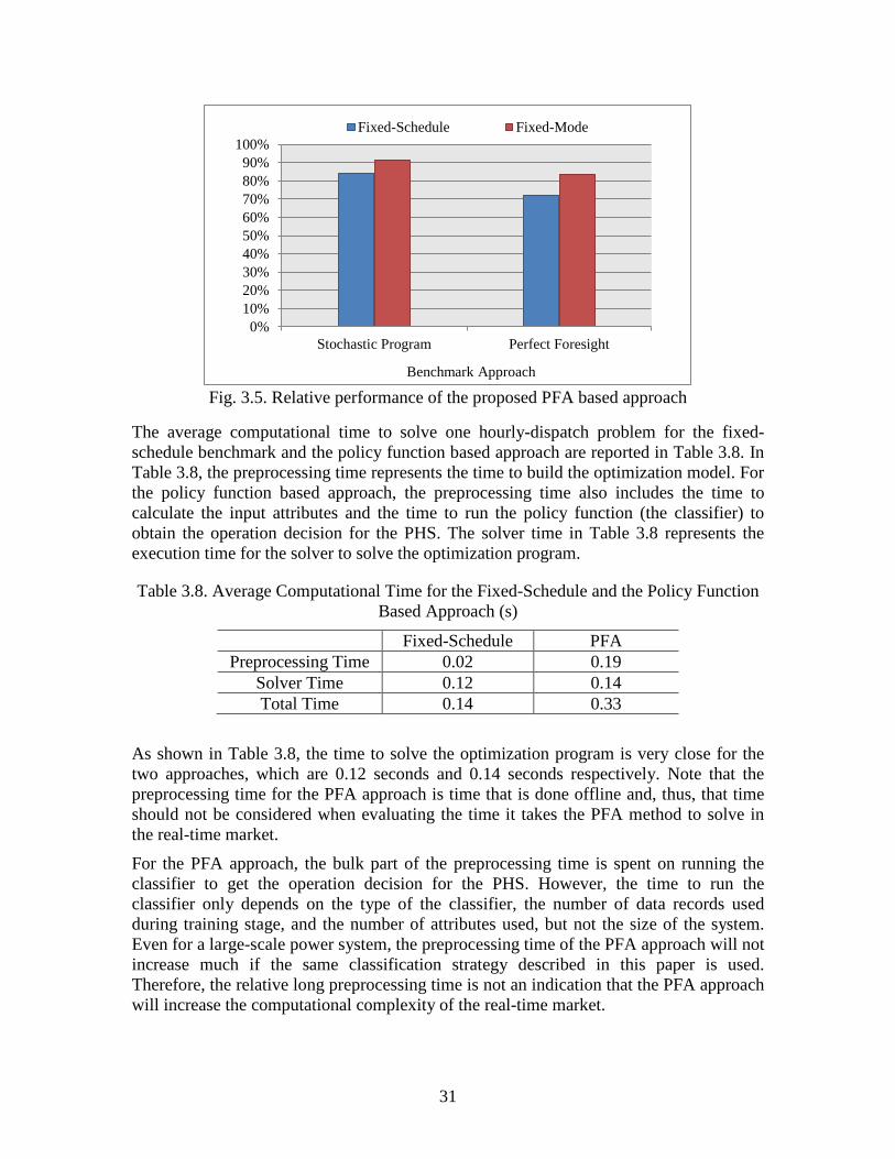
31

Fig. 3.5. Relative performance of the proposed PFA based approach

The average computational time to solve one hourly-dispatch problem for the fixed-schedule benchmark and the policy function based approach are reported in Table 3.8. In Table 3.8, the preprocessing time represents the time to build the optimization model. For the policy function based approach, the preprocessing time also includes the time to calculate the input attributes and the time to run the policy function (the classifier) to obtain the operation decision for the PHS. The solver time in Table 3.8 represents the execution time for the solver to solve the optimization program.

Table 3.8. Average Computational Time for the Fixed-Schedule and the Policy Function Based Approach (s)

Fixed-Schedule PFA Preprocessing Time 0.02 0.19

Solver Time 0.12 0.14 Total Time 0.14 0.33

As shown in Table 3.8, the time to solve the optimization program is very close for the two approaches, which are 0.12 seconds and 0.14 seconds respectively. Note that the preprocessing time for the PFA approach is time that is done offline and, thus, that time should not be considered when evaluating the time it takes the PFA method to solve in the real-time market.

For the PFA approach, the bulk part of the preprocessing time is spent on running the classifier to get the operation decision for the PHS. However, the time to run the classifier only depends on the type of the classifier, the number of data records used during training stage, and the number of attributes used, but not the size of the system. Even for a large-scale power system, the preprocessing time of the PFA approach will not increase much if the same classification strategy described in this paper is used. Therefore, the relative long preprocessing time is not an indication that the PFA approach will increase the computational complexity of the real-time market.

0%10%20%30%40%50%60%70%80%90%

100%

Stochastic Program Perfect Foresight

Benchmark Approach

Fixed-Schedule Fixed-Mode

32

The results in Fig. 3.5 and Table 3.8 demonstrate that the proposed PFA approach is effective in enhancing the utilization of the PHS in system with renewable resources.

Note that any such investigation is case specific; we do not anticipate that policy functions will have such performance for all the cases. With that said, the result has achieved our primary objective and agrees with our initial insight: while stochastic programming approaches are beneficial, they are computationally challenging, especially for real-time applications whereas policy functions are very effective and do not increase the computational complexity.

Finally, while the cost savings are not that high, note that this is for a single PHS facility, which is why it is important to acknowledge that we have saved roughly 70% to 90% of the overall potential cost savings. For systems with more PHS resources, the overall impact of this approach will be more profound.

Besides the benchmark approaches tested and compared in the case study, there are also other existing approaches that manage the state of charge (SOC) of energy storage across multiple time periods in real-time market. In [17] and [41],

3.9 Conclusion and Future Work

With the rapid expansion of renewable resources, there is a growing need for flexible resources in power systems. While energy storage has been considered a potential solution to manage the intermittency of renewable resources, the flexibility of energy storage is not being fully utilized by existing energy and market management systems. In this chapter, a policy function approximation based approach is proposed to enhance the utilization of pumped hydro storage in operation with limited look-ahead functionalities. The proposed PFA base approach is shown to be effective in improving the utilization of the PHS and have performance close to stochastic programming based methods. Meanwhile, compared to stochastic programming, the PFA based approach has minimal added computational difficulty.

While the policy function is developed for the operation of the PHS, the same design philosophy can be generalized to other power systems applications. As stochastic programming is still not scalable for large-scale power system today, the policy functions provide a solution to achieve the main functions of stochastic programming. The policy function has two primary merits:1) address the system uncertainties using the knowledge obtained during prior stages, and 2) has minimal added computational complexity to the existing management system.

Future work may extend the PFA based approach to a large-scale power system. For large-scale power systems, zonal partition techniques can be applied to divide the system into several zones based on congestion information, location of the PHS or the location of the wind farms. The PFA based approach can then be applied on a locational base to obtain the input attributes using the information within each zone.

Another direction is to compare the performance of the policy function based approach with other existing benchmark approaches that are not included in this chapter. One such benchmark approach is reported in [17] and [41]. In [17] and [41], a three-stage (day-ahead stage, hour-ahead stage and real-time stage) sequential simulation approach is

33

implemented to evaluate the benefits of adjustable-speed PHS. In each stage, the storage volume of a PHS at the end of the optimization window is constrained to the one determined from the previous stage. The storage volume constraint can be violated by a penalty price. The approach in [17] and [41] allows the PHS to deviate from the schedule determined from a previous stage by paying a penalty cost. As the policy function based approach is designed to be a practical method that can be implemented by the ISOs, a more comprehensive performance assessment can be obtained for the policy function based approach by comparing it with more benchmark approaches.

Directions for future work could also include extending the day-ahead stochastic simulation to an offline approach. With such strategies, PFAs can be generated on a weekly base or monthly base. By using historical data, the computational requirement is further reduced for the day-ahead stage. However, the shortcoming of generating PFAs based on historical data is that the performance of the PFA may be deteriorated, since the historical data may have less similarity and correlation with the future system operating conditions.

There is also potential to incorporate the PFAs into market structure. In deregulated energy markets, PHS entities are market participants who bid into the market and try to maximize their profits. To utilize PFAs in such market settings, the existing market structure may need to be redesigned such that enough incentive is provided for the PHS units to follow the dispatch instructions provided by the system operator.

34

4. Conclusions

In this report, the operation of pumped hydro storage (PHS) in systems with renewable resources is investigated. The report studies the attractiveness of two PHS technologies in balancing renewable uncertainties. A policy function based approach is proposed to improve the operational scheme of the PHS in real-time operation.

Two types of PHS technologies are studied in the report, which are the traditional fixed-speed PHS and the adjustable-speed PHS. As an advanced PHS technology, the adjustable-speed PHS is able to change its input power in the pumping mode, which provides it the capability to provide regulation reserves in both the generation and pumping mode. For the fixed-speed PHS, as the input power cannot be varied during the pumping process, the fixed-speed PHS can only provide regulation reserves in the generation mode. In the case study, the result shows that the adjustable-speed PHS is more effective in providing regulation reserves and reducing total system costs compared to the fixed-speed PHS. It is demonstrated in this report that the adjustable-speed PHS is a more attractive and valuable resource than the fixed-speed PHS to facilitate the integration of renewable resources

While studies have demonstrated the attractiveness of the PHS in managing the renewable uncertainties in the system, existing energy management systems and market management systems do not make full use of the flexibility of storage. In this report, a policy function based approach is proposed to enhance the utilization of the PHS in real-time operation. In the proposed approach, the policy function is generated on a daily base using the day-ahead wind forecasts. As stochastic programming models are not computational tractable for large-scale power systems, policy functions provide a scalable solution to address the challenges with the uncertainty and the limited look-ahead functionality in real-time operation. By shifting computational complexity to offline analysis, policy functions have minimal added computational difficulty to the existing energy management system. In the report, random forest classification technique is used to generate the policy function. The policy function is used to determine the pattern between the system operating conditions and the optimal decisions for the PHS. Compared to the existing approach where a fixed operational schedule is used, the result shows that the policy function based approach can effectively enhance the utilization of the PHS in real-time operation. The result also indicates that the policy function based approach has close performance to the stochastic programming model based benchmark and the perfect-foresight benchmark. By using the proposed approach, the PHS can be utilized more efficiently and more effectively to facilitate the integration of increasing penetrations of renewable resources.

35

References

[1] Global Wind Energy Council, “Global wind report: annual market update 2012,” April 2013. [Online]. Available: http://www.gwec.net/wp-content/uploads/2012/06/Annual_report_2012_LowRes.pdf

[2] World Wind Energy Association,”2012 Half-year report,” [Online]. Available: http://www.wwindea.org/webimages/Half-year_report_2012.pdf

[3] Earth Techling, “Global solar, wind energy growth continues to impress,” [Online]. Available: http://www.earthtechling.com/2013/07/global-solar-wind-energy-growth-continues-to-impress/

[4] Energy Information Administration, “Most states have renewable portfolio standards,” February 2012. [Online]. Available: http://www.eia.gov/todayinenergy/detail.cfm?id=4850

[5] Energy Information Administration, “Existing capacity by energy source,” 2012. [Online]. Available: http://www.eia.gov/electricity/annual/html/epa_04_03.html

[6] M. Kintner-Meyer, et al., “Energy storage for power system applications: a regional assessment for the northwest power pool,” PNNL, Richland, WA. April, 2010. [Online.] Available: http://www.pnl.gov/main/publications/external/technical_reports/PNNL-19300.pdf.

[7] Electric Power Research Institute, “Electricity energy storage technology options – a white paper primer on applications, costs, and benefits,” December 2010. [Online]. Available: http://www.electricitystorage.org/images/uploads/static_content/technology/resources/ESA_TR_5_11_EPRIStorageReport_Rastler.pdf

[8] R. Sioshansi, P. Denholm, T. Jenkin, and J. Weiss, “Estimating the value of electricity storage in PJM: arbitrage and some welfare effects,” Energy Economics, vol. 32, no. 2, pp. 269-277, March 2009.

[9] R. Walawalkar, J. Apt, and R. Mancini, “Economics of electric energy storage for energy arbitrage and regulation in New York,” Energy Policy, vol. 35, no. 4, pp. 2558-2568, November 2006.

[10] G. Gross, A. Dominguez-Garcia, C. Singh, and A. Sprintson, “Integration of storage devices into power systems with renewable energy sources,” PSERC Publication 12-24, September 2012. [Online]. Available: http://www.pserc.wisc.edu/documents/publications/reports/2012_reports/gross_pserc_project_s-40_2012.pdf

[11] A. Tuohy, M. O’Malley, “Impact of pumped storage on power system with increasing wind penetration,” IEEE Power & Energy Society General Meeting, July 2009.

36

[12] J. P. Deane, E. J. Mckeogh, and B. P. O. Gallachoir, “Derivation of intertemporal targets for large hydro energy storage with stochastic optimization,” IEEE Transactions on Power Systems, vol. 28, no. 3, pp. 2147-2155, August 2013.

[13] M. E. Khodayar and M. Shahidehpour, “Enhancing the dispatchability of variable wind generation by coordination with pumped-storage hydro units in stochastic power systems,” IEEE Transactions on Power Systems, vol. 28, no. 3, pp. 2808-2818, August 2013.

[14] N. Li and K. Hedman, “Economic assessment of energy storage in systems with high levels of renewable resources,” IEEE Transactions on Sustainable Energy, accepted for publication.

[15] National Hydropower Association, “Challenges and opportunities for new pumped storage development,” [Online]. Available: http://www.hydro.org/wp-content/uploads/2012/07/NHA_PumpedStorage_071212b1.pdf

[16] V. Koritarov, et al., “Modeling ternary pumped hydro storage units,” Argonne National Laboratory, August 2013. [Online]. Available: http://www.ipd.anl.gov/anlpubs/2013/10/77293.pdf

[17] V. Koritarov, et al., “Modeling and analysis of value of advanced pumped hydro storage hydropower in the United States,” Argonne National Laboratory, June 2014. [Online]. Available: http://www.dis.anl.gov/projects/psh/ANL-DIS-14-7_Advanced_PSH_Final_Report.pdf

[18] GE Energy, “Western wind and solar integration study,” National Renewable Energy Laboratory, May 2010. [Online]. Available: http://www.nrel.gov/docs/fy10osti/47434.pdf

[19] X. Ma, H. Song, M. Hong, J. W, Y. Chen, and E. Zak, “The security-constrained commitment and dispatch for Midwest ISO day-ahead co-optimized energy and ancillary service market,” IEEE Power & Energy Society General Meeting, July 2009.

[20] X. Ma, Y. Chen, and J. Wan, “Midwest ISO co-optimization based real-time dispatch and pricing of energy and ancillary services,” IEEE Power & Energy Society General Meeting, July 2009.

[21] University of Washington, “Power systems test case archive,” Dept. Elect. Eng., 1999. [Online]. Available: http://www.ee.washington.edu/research/pstca/rts/pg tcarts.htm

[22] J. M. S. Pinheiro, C. R. R. Dornellas, M. Th. Schilling, A. C. G. Melo, and J. C. O. Mello, “Probing the new IEEE reliability test system (RTS-96): HL-II Assessment,” IEEE Transactions on Power Systems, vol. 13, no. 1, pp. 171-176, February 1998.

[23] J. D. Lyon, F. Wang, K. W. Hedman, and M. Zhang, “Market implications and pricing of dynamic reserve policies for systems with renewables,” IEEE Transactions on Power Systems, accepted for publication.

37

[24] J. M. Morales, R. Minguez, and A. J. Conejo, “A methodology to generate statistically dependent wind speed scenarios,” Applied Energy, vol. 87, pp. 843–855, September 2009.

[25] National Renewable Energy Laboratory, “Wind integration datasets,” 2006. [Online]. Available: http://www.nrel.gov/electricity/transmission/wind_integration_dataset.html

[26] California Public Utilities Commission, “CPUC sets energy storage goals for utilities,” 2013. [Online]. Available: http://docs.cpuc.ca.gov/PublishedDocs/Published/G000/M079/K171/79171502.PDF

[27] Electric Power Research Institute, “Electricity energy storage technology options – a white paper primer on applications, costs, and benefits,” December 2010. [Online]. Available: http://www.electricitystorage.org/images/uploads/static_content/technology/resources/ESA_TR_5_11_EPRIStorageReport_Rastler.pdf

[28] R. E. Bellman, Dynamic Programming. Princeton, NJ: Princeton University Press, 2003.

[29] W. B. Powell, Approximate Dynamic Programming: Solving the Curses of Dimensionality, 2nd ed. New York: Wiley, 2001.

[30] P. Tan, M. Steinbach, and V. Kumar, Introduction to Data Mining 1st edition. Boston, MA: Addison-Wesley, 2006.

[31] K. Sun, S. Likhate, V. Vittal, S. Kolluri, S. Mandal, "An online dynamic security assessment scheme using phasor measurements and decision trees", IEEE Transactions on Power Systems, vol. 22, no. 4, pp. 1935-1943, November 2007.

[32] Y. Zhang, M. Ilic, and O. Tonguz, “Application of support vector machine classification to enhanced protection relay logic in electric power grids,” 2007 Large Engineering Systems Conference on Power Engineering, pp. 31-38, October 2007.

[33] D. Srinivasan, W. S. Ng, and A. C. Liew, “Neural-network based signature recognition for harmonic source identification,” IEEE Transactions on Power Delivery, vol. 2, no. 1, pp. 398-405, January 2006.

[34] C. N. Sillar Jr., and A. A. Freitas, “A survey of hierarchical classification across different application domains,” Data Mining and Knowledge Discovery, vol. 22, no. 1-2, pp. 31-72, January 2011.

[35] L. Breiman, “Random forests,” Machine Learning, vol. 45, no. 1, pp. 5-32, October 2001.

[36] C. Hsu, C. Chang, and C. Lin, “A practical guide to support vector machine,” National Taiwan University, April 2010. [Online]. Available: http://www.csie.ntu.edu.tw/~cjlin/papers/guide/guide.pdf

[37] W. Yuan-Kang and H. Jing-Shan, “A literature review of wind forecasting technology in the world,” Proc. IEEE Power Tech, pp. 504 -509, July 2007.

38

[38] S. Fan, J. R. Liao, R. Yokoyama, L. Chen, and W. Lee, “Forecasting the wind generation using a two-stage network based on meteorological information,” IEEE Transactions on Energy Conversion, vol. 24, no. 2, pp. 474-482, June 2009.

[39] Pedregosa et al., “Scikit-learn: machine learning in Python,” Journal of Machine Learning Research, vol. 12, pp. 2825-2830, October 2011.

[40] J. Dupacová, N. Gröwe-Kuska, and W. Römisch, “Scenario reduction in stochastic programming: an approach using probability metrics,” Mathematical Programming, Series A, vol. 3, pp. 493–511, February 2003.

[41] T. Guo, et al., “Adjustable speed pumped-storage hydro-generator (PSH) evaluation by PLEXOS,” Energy Exemplar, LLC, Roseville, CA, Tech. Rep. EE-2013-10-30-01, October 2013.