Embed Size (px)
Citation preview
PRODUCTION FORECAST & DECLINE CURVES
DAY 3 AFTERNOON
PRODUCTION FORECAST & DECLINE CURVES
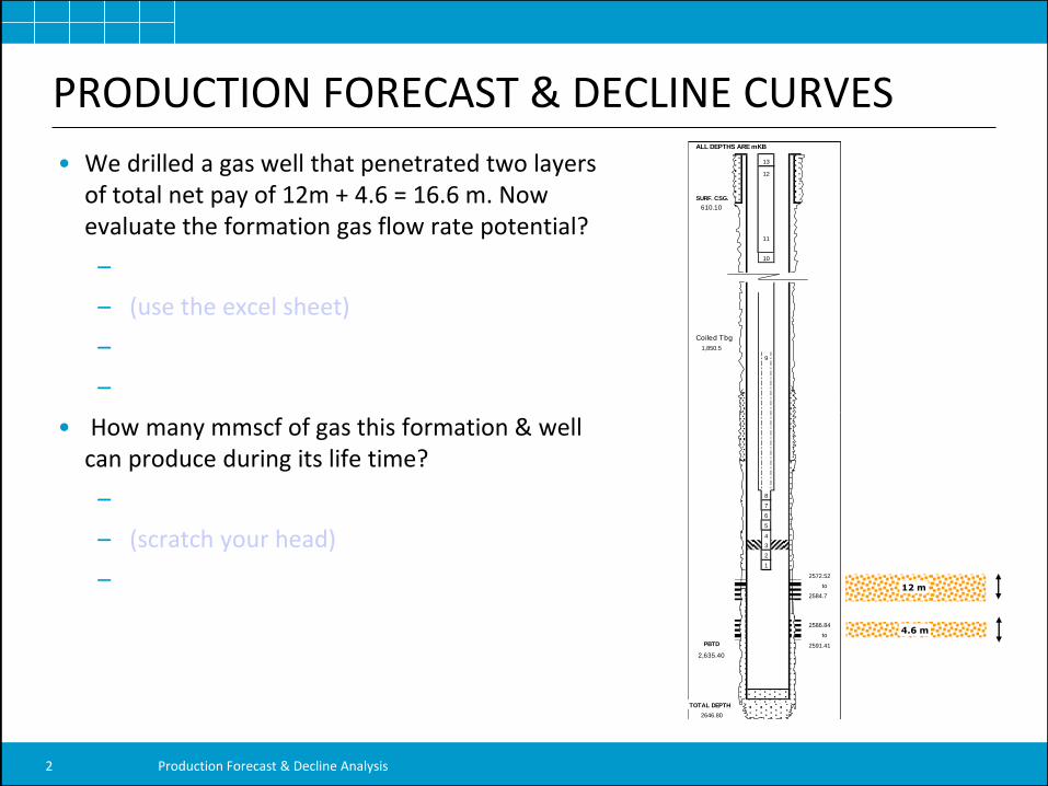
• We drilled a gas well that penetrated two layers of total net pay of 12m + 4.6 = 16.6 m. Now evaluate the formation gas flow rate potential?
–
– (use the excel sheet)
–
–
• How many mmscf of gas this formation & well can produce during its life time?
–
– (scratch your head)
–
ALL DEPTHS ARE mKB
13
12
SURF. CSG.
610.10
11
10
- from bottom up -
Coiled Tbg
1,850.5
9
8
7
6
5
4
3
2
1
2572.52
to
2584.7
2586.84
to
PBTD 2591.41
2,635.40
TOTAL DEPTH
2646.80
12 m
4.6 m
Production Forecast & Decline Analysis 2
PRODUCTION FORECAST & DECLINE CURVES
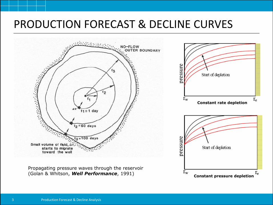
Propagating pressure waves through the reservoir (Golan & Whitson, Well Performance, 1991)
Constant rate depletion
Constant pressure depletion
Production Forecast & Decline Analysis 3
OBJECTIVES OF PRODUCTION FORECASTING
• For new wells
– Estimate well’s initial rate
– Assess well’s total production volume during its life
• For current producers
– Calculate remaining recoverable reserves
– Calculate original recoverable reserves
• For managing reservoir development
– Observe reservoir behavior, independently of operational activities
– Observe interwell communication
• For base management
– Detect operational problems
Production Forecast & Decline Analysis 4
PRODUCTION FORECAST & DECLINE CURVES
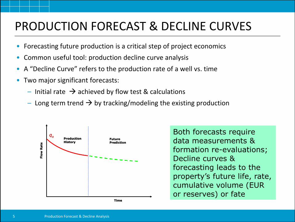
• Forecasting future production is a critical step of project economics
• Common useful tool: production decline curve analysis
• A “Decline Curve” refers to the production rate of a well vs. time
• Two major significant forecasts:
– Initial rate achieved by flow test & calculations
– Long term trend by tracking/modeling the existing production
Production History
Future Prediction
Flo
w R
ate
qo
Time
Production History
Future Prediction
Flo
w R
ate
qo
Time
Both forecasts require data measurements & formation re-evaluations; Decline curves & forecasting leads to the property’s future life, rate, cumulative volume (EUR or reserves) or fate
Production Forecast & Decline Analysis 5
PRODUCTION FORECAST & DECLINE CURVES
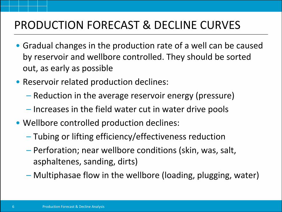
• Gradual changes in the production rate of a well can be caused by reservoir and wellbore controlled. They should be sorted out, as early as possible
• Reservoir related production declines:
– Reduction in the average reservoir energy (pressure)
– Increases in the field water cut in water drive pools
• Wellbore controlled production declines:
– Tubing or lifting efficiency/effectiveness reduction
– Perforation; near wellbore conditions (skin, was, salt, asphaltenes, sanding, dirts)
– Multiphasae flow in the wellbore (loading, plugging, water)
Production Forecast & Decline Analysis 6
PRODUCTION FORECAST & DECLINE CURVES
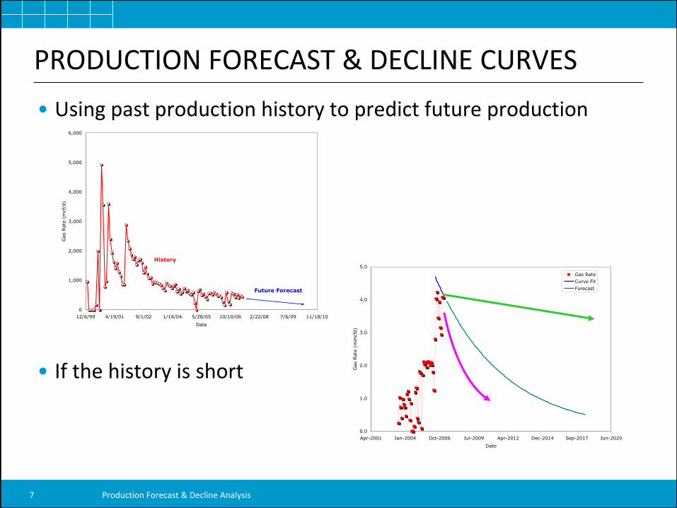
• Using past production history to predict future production
• If the history is short
0
1,000
2,000
3,000
4,000
5,000
6,000
12/6/99 4/19/01 9/1/02 1/14/04 5/28/05 10/10/06 2/22/08 7/6/09 11/18/10
Date
Gas R
ate
(m
cf/
d)
History
Future Forecast
Production Forecast & Decline Analysis 7
0.0
1.0
2.0
3.0
4.0
5.0
Apr-2001 Jan-2004 Oct-2006 Jul-2009 Apr-2012 Dec-2014 Sep-2017 Jun-2020
Date
Gas R
ate
(m
mcfd
)
Gas Rate
Curve Fit
Forecast
PRODUCTION FORECAST & DECLINE CURVES
• Once production begins, oil, gas, sometimes water, are flowing out of a reservoir, reservoir energy will be depleted, causing the production to decline.
• Decline trends are manifested by seeing a declining well head gas rate, oil rate, or a declining wellhead pressure or bottomhole pressure, or an increasing water-oil ratio (WOR), or a surge of production gas-oil ratio.
• Decline patterns are controlled by reservoir size, energy level, flowing rate, formation characteristics, fluid properties, and operating conditions.
• All wells, reservoirs, and fields, will exhibit production decline trend, as more hydrocarbons have been evacuated from a reservoir of fixed volume, structurally or stratigraphically.
Production Forecast & Decline Analysis 8
ARPS DECLINE ANALYSIS
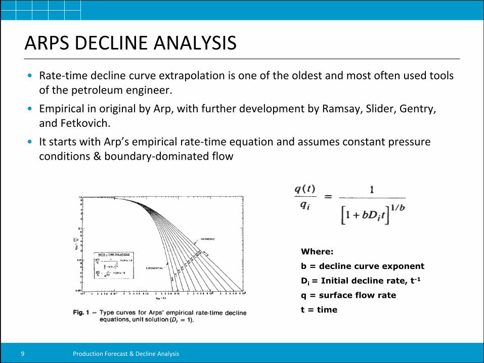
• Rate-time decline curve extrapolation is one of the oldest and most often used tools of the petroleum engineer.
• Empirical in original by Arp, with further development by Ramsay, Slider, Gentry, and Fetkovich.
• It starts with Arp’s empirical rate-time equation and assumes constant pressure conditions & boundary-dominated flow
Where:
b = decline curve exponent
Di = Initial decline rate, t-1
q = surface flow rate
t = time
Production Forecast & Decline Analysis 9
ARPS DECLINE ANALYSIS
• Early work by J.J. Arps (1945) from his field observations: – Exponential Decline
– Hyperbolic Decline
– Harmonic Decline
• Commonly called “Curve Fitting”; empirically established from wells or fields or pools
• Advantages:
– Easy to analyze and to forecast » Widely used in reserve evaluation & forecast due to its simplicity
• Disadvantages
– Too empirical, without thorough theoretical justification or in-depth understanding
Production Forecast & Decline Analysis 10
ARPS DECLINE ANALYSIS
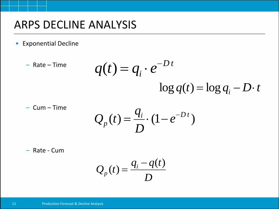
• Exponential Decline
– Rate – Time
– Cum – Time
– Rate - Cum
)1()( tDip e
D
qtQ
tD
i eqtq )(
tDqtq i log)(log
D
tqqtQ i
p
)()(
Production Forecast & Decline Analysis 11
ARPS DECLINE ANALYSIS
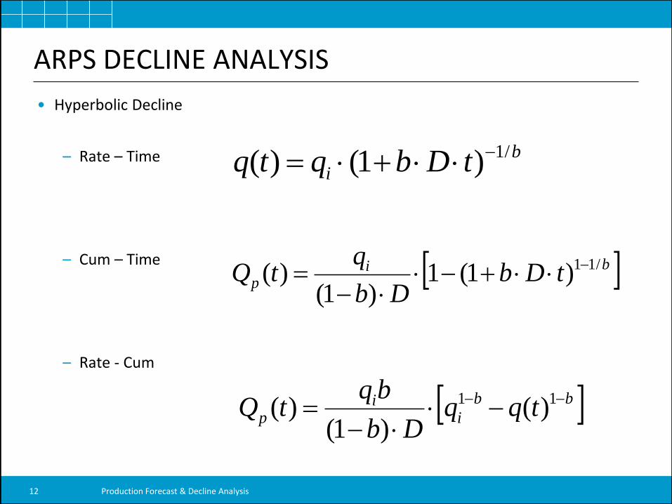
• Hyperbolic Decline
– Rate – Time
– Cum – Time
– Rate - Cum
bip tDb
Db
qtQ /11)1(1
)1()(
b
i tDbqtq /1)1()(
bb
ii
p tqqDb
bqtQ
11 )(
)1()(
Production Forecast & Decline Analysis 12
ARPS DECLINE ANALYSIS
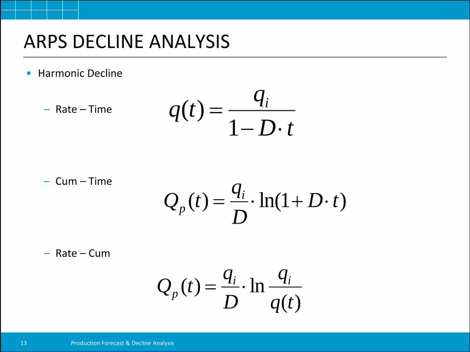
• Harmonic Decline
– Rate – Time
– Cum – Time
– Rate – Cum
)1ln()( tDD
qtQ i
p
tD
qtq i
1)(
)(ln)(
tq
q
D
qtQ ii
p
Production Forecast & Decline Analysis 13
ARPS DECLINE ANALYSIS
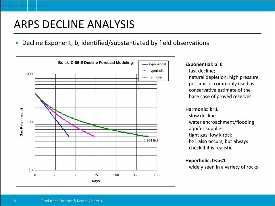
• Decline Exponent, b, identified/substantiated by field observations
Buick C-86-E Decline Forecast Modeling
10
100
1000
0 25 50 75 100 125 150
Days
Ga
s R
ate
(m
sc
fd)
exponential
hyperbolic
harmonic
0.164 Bcf
Exponential: b=0 fast decline; natural depletion; high pressure pessimistic commonly used as conservative estimate of the base case of proved reserves Harmonic: b=1 slow decline water encroachment/flooding aquifer supplies tight gas; low k rock b>1 also occurs, but always check if it is realistic Hyperbolic: 0<b<1 widely seen in a variety of rocks
Production Forecast & Decline Analysis 14
PRODUCTION FORECAST & DECLINE CURVES
Production Forecast & Decline Analysis 15
ARPS DECLINE ANALYSIS
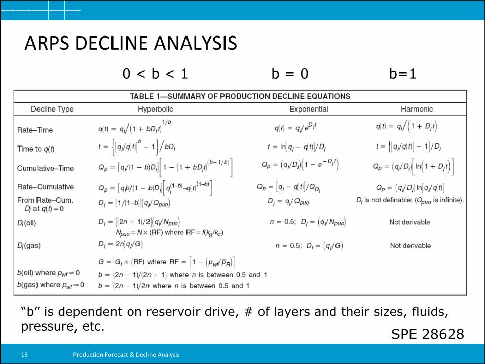
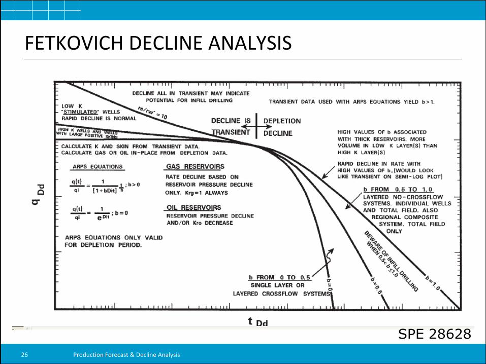
SPE 28628
0 < b < 1 b = 0 b=1
“b” is dependent on reservoir drive, # of layers and their sizes, fluids, pressure, etc.
Production Forecast & Decline Analysis 16
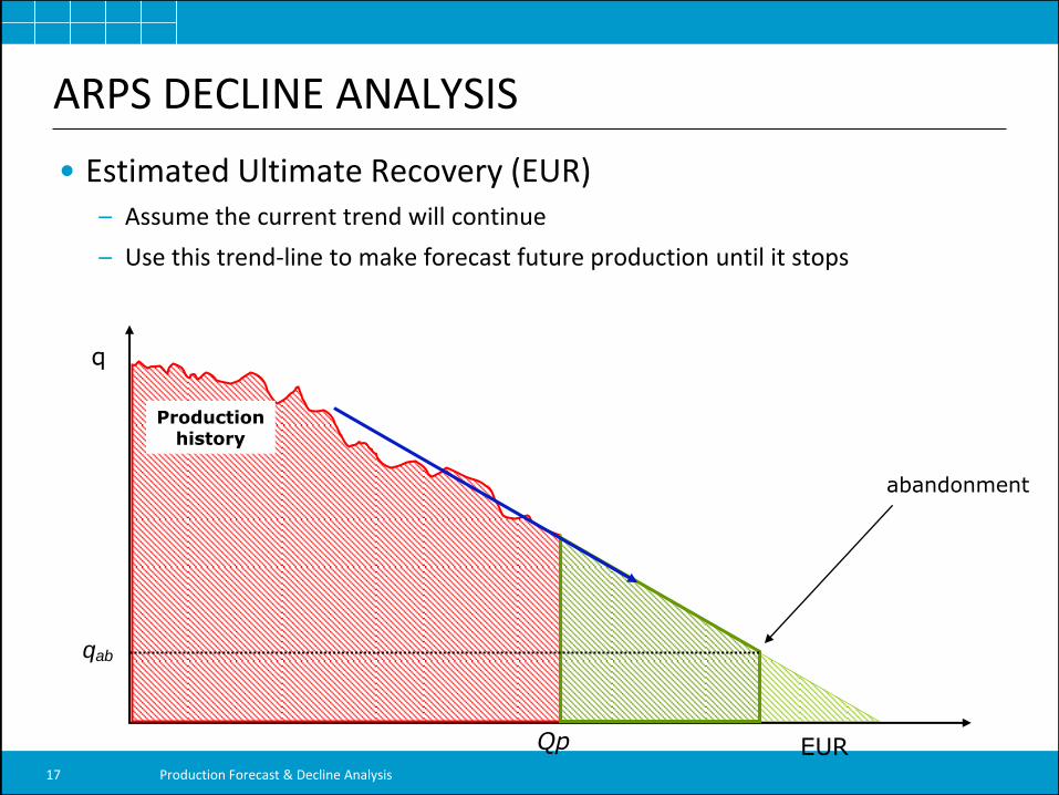
• Estimated Ultimate Recovery (EUR) – Assume the current trend will continue
– Use this trend-line to make forecast future production until it stops
ARPS DECLINE ANALYSIS
q
Qp EUR
qab
abandonment
Production history
Production Forecast & Decline Analysis 17
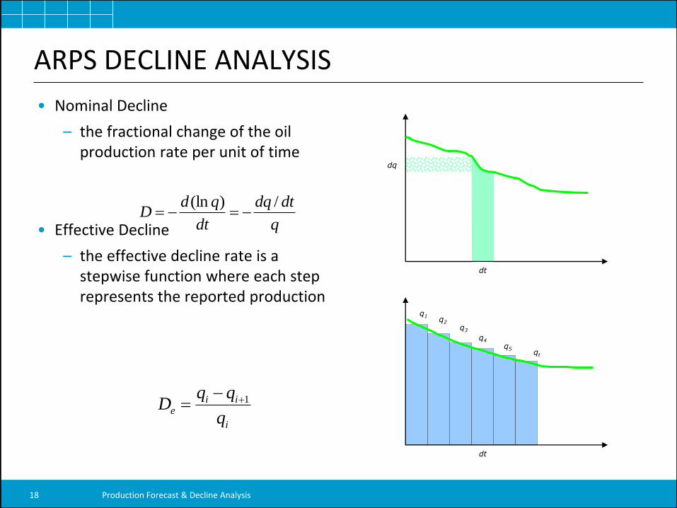
ARPS DECLINE ANALYSIS
• Nominal Decline
– the fractional change of the oil production rate per unit of time
• Effective Decline
– the effective decline rate is a stepwise function where each step represents the reported production
q
dtdq
dt
qdD
/)(ln
dq
dt
q1
dt
q2
q3
q4
q5 qt
i
iie
q
qqD 1
Production Forecast & Decline Analysis 18
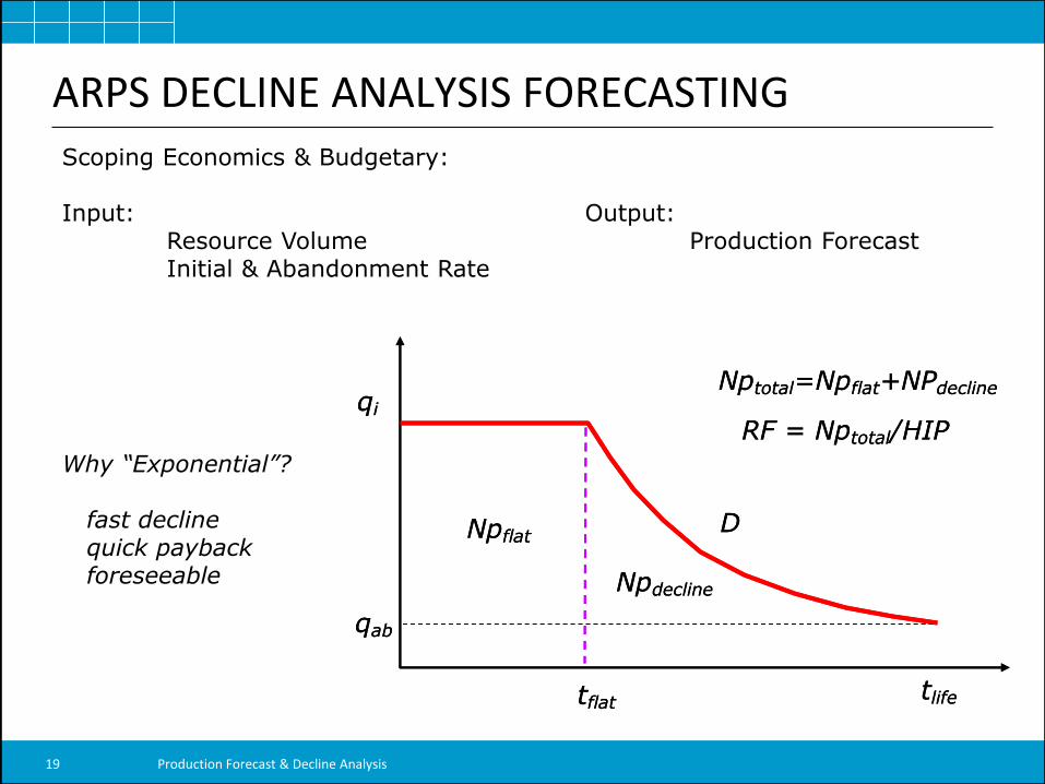
ARPS DECLINE ANALYSIS FORECASTING
qi
tflat
qab
tlife
DNpflat
Npdecline
Nptotal=Npflat+NPdecline
RF = Nptotal/HIPqi
tflat
qab
tlife
DNpflat
Npdecline
Nptotal=Npflat+NPdecline
RF = Nptotal/HIP
Scoping Economics & Budgetary: Input: Output: Resource Volume Production Forecast Initial & Abandonment Rate Why “Exponential”? fast decline quick payback foreseeable
Production Forecast & Decline Analysis 19
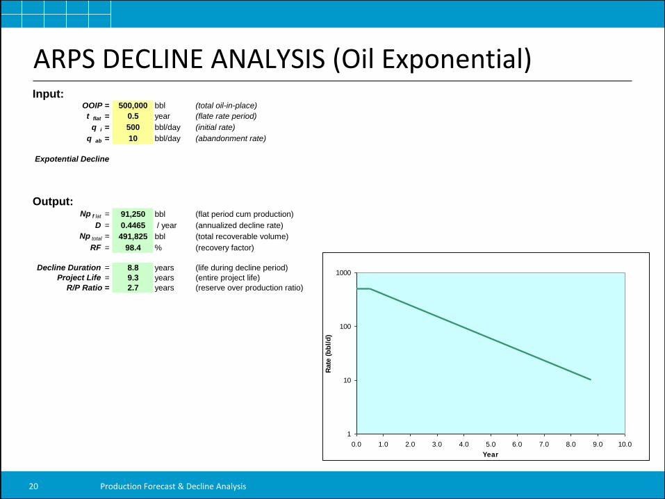
ARPS DECLINE ANALYSIS (Oil Exponential)
1
10
100
1000
0.0 1.0 2.0 3.0 4.0 5.0 6.0 7.0 8.0 9.0 10.0
Year
Rate
(b
bl/
d)
Input:OOIP = 500,000 bbl (total oil-in-place)
t flat = 0.5 year (flate rate period)
q i = 500 bbl/day (initial rate)
q ab = 10 bbl/day (abandonment rate)
Expotential Decline
Output:Np f lat = 91,250 bbl (flat period cum production)
D = 0.4465 / year (annualized decline rate)
Np total = 491,825 bbl (total recoverable volume)
RF = 98.4 % (recovery factor)
Decline Duration = 8.8 years (life during decline period)
Project Life = 9.3 years (entire project life)
R/P Ratio = 2.7 years (reserve over production ratio)
Production Forecast & Decline Analysis 20
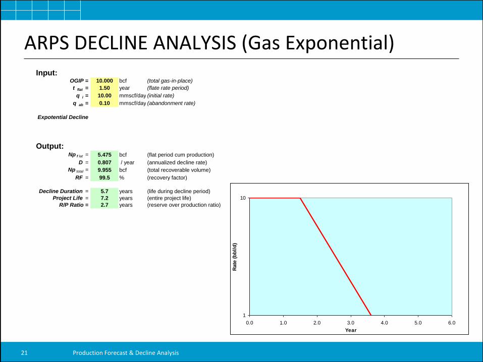
ARPS DECLINE ANALYSIS (Gas Exponential) Input:
OGIP = 10.000 bcf (total gas-in-place)
t flat = 1.50 year (flate rate period)
q i = 10.00 mmscf/day (initial rate)
q ab = 0.10 mmscf/day (abandonment rate)
Expotential Decline
Output:Np f lat = 5.475 bcf (flat period cum production)
D = 0.807 / year (annualized decline rate)
Np total = 9.955 bcf (total recoverable volume)
RF = 99.5 % (recovery factor)
Decline Duration = 5.7 years (life during decline period)
Project Life = 7.2 years (entire project life)
R/P Ratio = 2.7 years (reserve over production ratio)
1
10
0.0 1.0 2.0 3.0 4.0 5.0 6.0
Year
Ra
te (
bb
l/d
)
1
10
0.0 1.0 2.0 3.0 4.0 5.0 6.0
Year
Rate
(b
bl/
d)
Production Forecast & Decline Analysis 21
PRODUCTION FORECAST & DECLINE CURVES
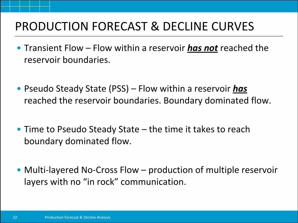
• Transient Flow – Flow within a reservoir has not reached the reservoir boundaries.
• Pseudo Steady State (PSS) – Flow within a reservoir has reached the reservoir boundaries. Boundary dominated flow.
• Time to Pseudo Steady State – the time it takes to reach boundary dominated flow.
• Multi-layered No-Cross Flow – production of multiple reservoir layers with no “in rock” communication.
Production Forecast & Decline Analysis 22
PRODUCTION DECLINE ANALYSIS
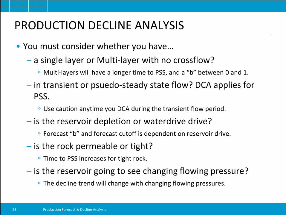
• You must consider whether you have…
– a single layer or Multi-layer with no crossflow? » Multi-layers will have a longer time to PSS, and a “b” between 0 and 1.
– in transient or psuedo-steady state flow? DCA applies for PSS. » Use caution anytime you DCA during the transient flow period.
– is the reservoir depletion or waterdrive drive? » Forecast “b” and forecast cutoff is dependent on reservoir drive.
– is the rock permeable or tight? » Time to PSS increases for tight rock.
– is the reservoir going to see changing flowing pressure? » The decline trend will change with changing flowing pressures.
Production Forecast & Decline Analysis 23

Advanced Production Data Analysis & Forecasting
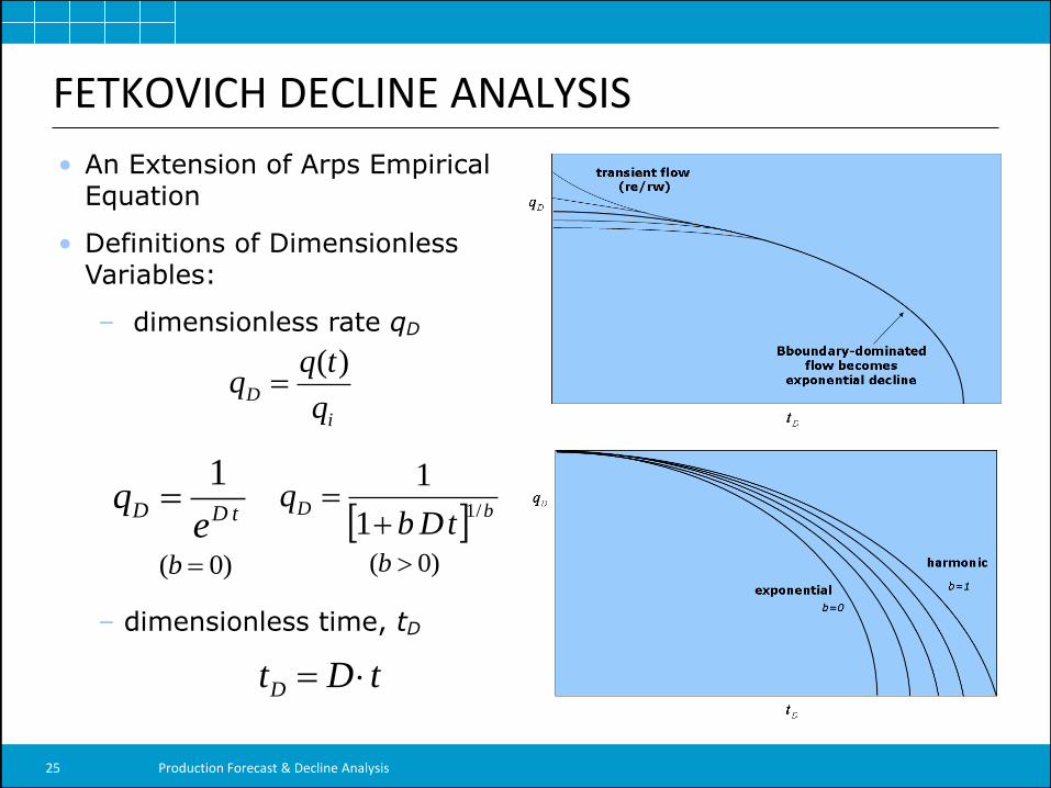
• An Extension of Arps Empirical Equation
• Definitions of Dimensionless Variables:
– dimensionless rate qD
– dimensionless time, tD
FETKOVICH DECLINE ANALYSIS
i
Dq
tqq
)(
tDtD
tDDe
q1
bD
tDbq
/11
1
tDtD
)0( b)0( b
Production Forecast & Decline Analysis 25
FETKOVICH DECLINE ANALYSIS
SPE 28628
Production Forecast & Decline Analysis 26
FETKOVICH DECLINE ANALYSIS
0
1000
2000
3000
4000
5000
6000
7000
8000
9000
0 100 200 300 400 500 600
Days of Production
Gas R
ate
0
200
400
600
800
1000
1200
1400
1600
Cum
Gas
10
100
1000
10000
10 100 1000
Days of Production
Gas R
ate
10
100
1000
10000
Cum
Gas
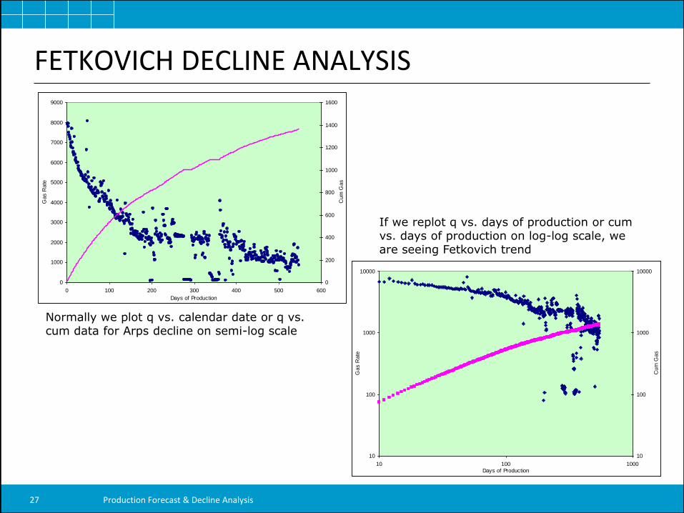
Normally we plot q vs. calendar date or q vs. cum data for Arps decline on semi-log scale
If we replot q vs. days of production or cum vs. days of production on log-log scale, we are seeing Fetkovich trend
Production Forecast & Decline Analysis 27
PRODUCTION FORECAST & DECLINE CURVES
1.E+03
1.E+04
1.E+05
1.E+06
1.E-03 1.E-02 1.E-01 1.E+00 1.E+01
tDd
qD
d
1.E+00
1.E+01
1.E+02
1.E+03
QD
d
)](
)(
[
]5.
0)
/[ln(
)(
300
,50
wf
pi
psc
weff
esc
Dd
PP
PP
hk
T
rr
TP
tq
q
]5.0)/[ln(]1)/[(5.0
/00633.02
2
weffeweffe
wefftg
Ddrrrr
rCtkt
)]()([)(
)(8.63722
wfpipwetgsc
psc
DdPPPPrrChT
tGTPQ
Production Forecast & Decline Analysis 28
FETKOVICH DECLINE ANALYSIS
)]()([
]2
1)[ln(1422
wfi
wa
e
MPDd
g
pmpmh
r
rT
q
qk
)]()([)(
54.56
wfiitMPDd
g
MPDd
ppmpmc
T
q
q
t
tV
gi
wp
B
SVOGIP
000,1
)1(
Production Forecast & Decline Analysis 29
PRODUCTION DECLINE ANALYSIS
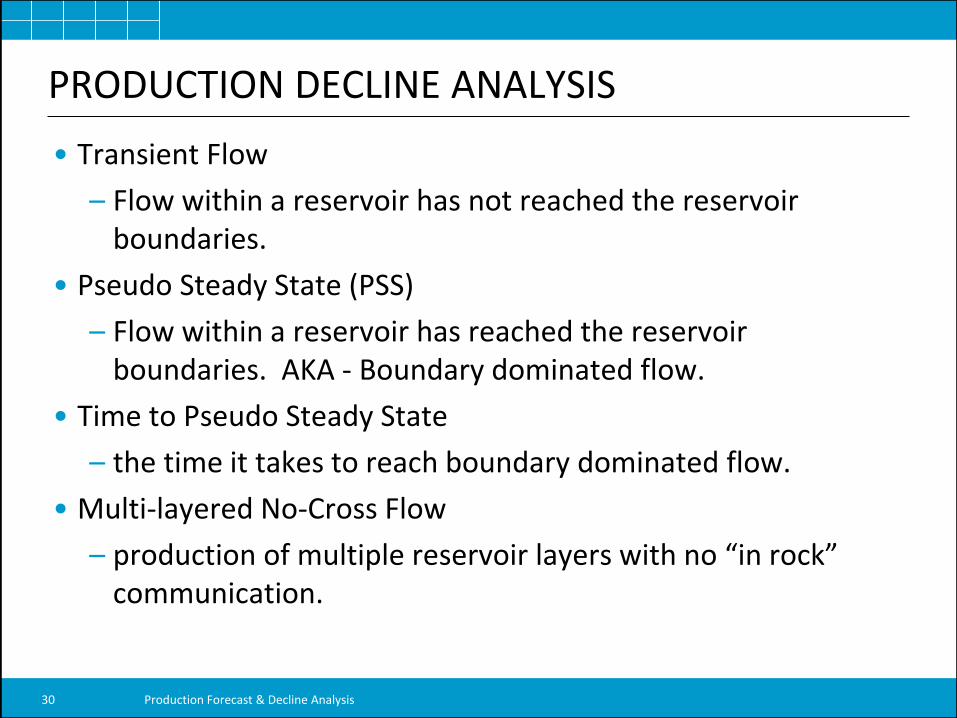
• Transient Flow
– Flow within a reservoir has not reached the reservoir boundaries.
• Pseudo Steady State (PSS)
– Flow within a reservoir has reached the reservoir boundaries. AKA - Boundary dominated flow.
• Time to Pseudo Steady State
– the time it takes to reach boundary dominated flow.
• Multi-layered No-Cross Flow
– production of multiple reservoir layers with no “in rock” communication.
Production Forecast & Decline Analysis 30
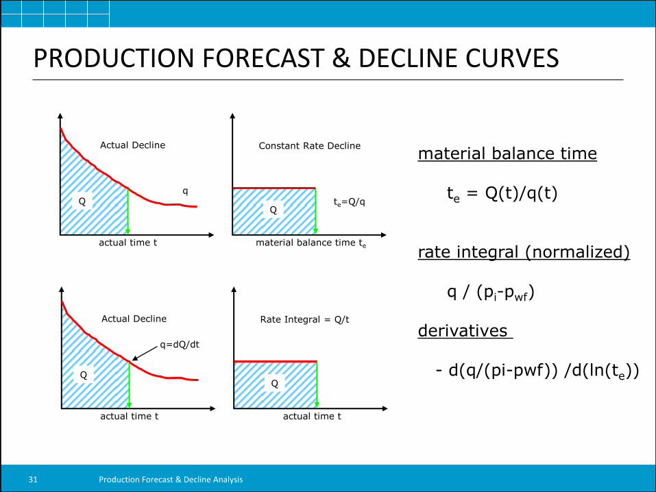
PRODUCTION FORECAST & DECLINE CURVES
actual time t
q
material balance time te
Q Q
te=Q/q
Constant Rate Decline Actual Decline
actual time t
q=dQ/dt
actual time t
Q Q
Rate Integral = Q/t Actual Decline
material balance time te = Q(t)/q(t) rate integral (normalized) q / (pi-pwf) derivatives - d(q/(pi-pwf)) /d(ln(te))
Production Forecast & Decline Analysis 31
ADVANCED VARIABLE RATES/PRESSURES
Production Forecast & Decline Analysis 32
FLOWING MATERIAL BALANCE
Production Forecast & Decline Analysis 33
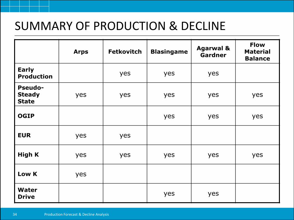
SUMMARY OF PRODUCTION & DECLINE
Arps Fetkovitch Blasingame Agarwal & Gardner
Flow Material Balance
Early Production
yes yes yes
Pseudo-Steady State
yes yes yes yes yes
OGIP yes yes yes
EUR yes yes
High K yes yes yes yes yes
Low K yes
Water Drive
yes yes
Production Forecast & Decline Analysis 34
W-83 Well/Pool Production Data Analysis
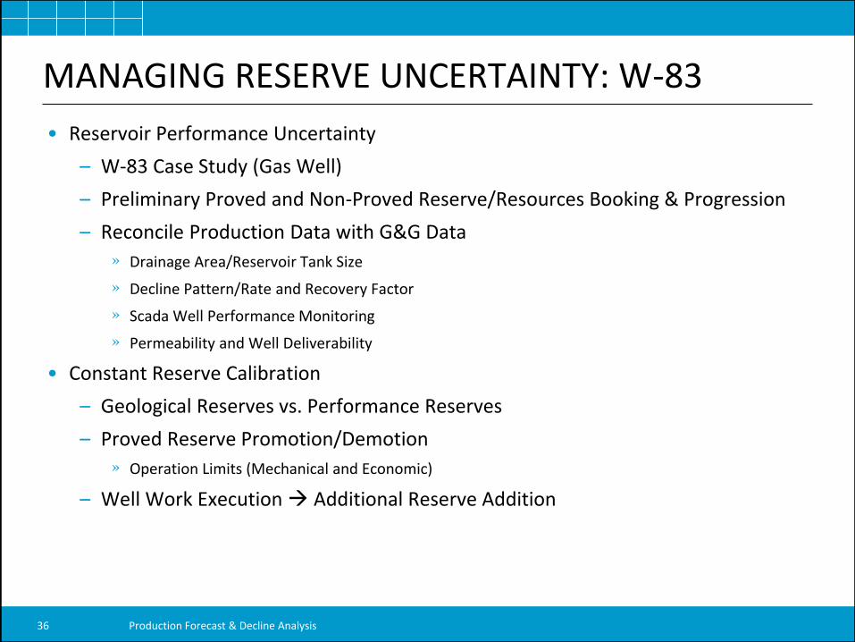
MANAGING RESERVE UNCERTAINTY: W-83
• Reservoir Performance Uncertainty
– W-83 Case Study (Gas Well)
– Preliminary Proved and Non-Proved Reserve/Resources Booking & Progression
– Reconcile Production Data with G&G Data
» Drainage Area/Reservoir Tank Size
» Decline Pattern/Rate and Recovery Factor
» Scada Well Performance Monitoring
» Permeability and Well Deliverability
• Constant Reserve Calibration
– Geological Reserves vs. Performance Reserves
– Proved Reserve Promotion/Demotion
» Operation Limits (Mechanical and Economic)
– Well Work Execution Additional Reserve Addition
Production Forecast & Decline Analysis 36
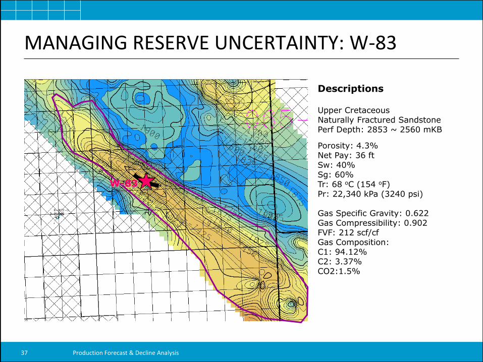
Descriptions Upper Cretaceous Naturally Fractured Sandstone Perf Depth: 2853 ~ 2560 mKB
Porosity: 4.3% Net Pay: 36 ft Sw: 40% Sg: 60% Tr: 68 oC (154 oF) Pr: 22,340 kPa (3240 psi) Gas Specific Gravity: 0.622 Gas Compressibility: 0.902 FVF: 212 scf/cf Gas Composition: C1: 94.12% C2: 3.37% CO2:1.5%
W-83
MANAGING RESERVE UNCERTAINTY: W-83
Production Forecast & Decline Analysis 37
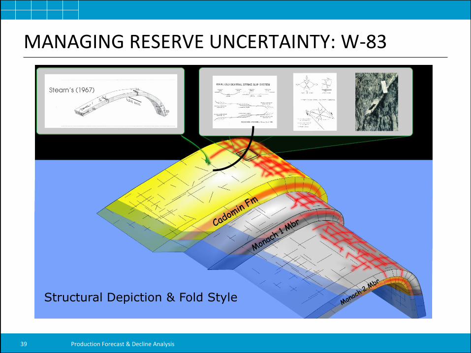
MANAGING RESERVE UNCERTAINTY: W-83
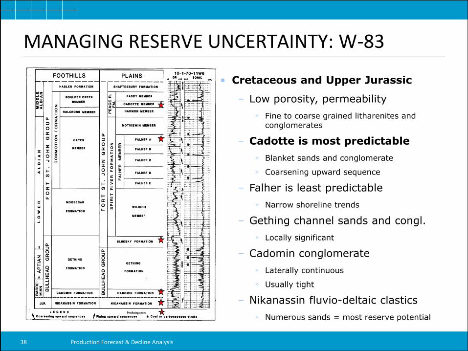
Producing zones
• Cretaceous and Upper Jurassic
– Low porosity, permeability
» Fine to coarse grained litharenites and conglomerates
– Cadotte is most predictable
» Blanket sands and conglomerate
» Coarsening upward sequence
– Falher is least predictable
» Narrow shoreline trends
– Gething channel sands and congl.
» Locally significant
– Cadomin conglomerate
» Laterally continuous
» Usually tight
– Nikanassin fluvio-deltaic clastics
» Numerous sands = most reserve potential
Production Forecast & Decline Analysis 38
MANAGING RESERVE UNCERTAINTY: W-83
Structural Depiction & Fold Style
Production Forecast & Decline Analysis 39
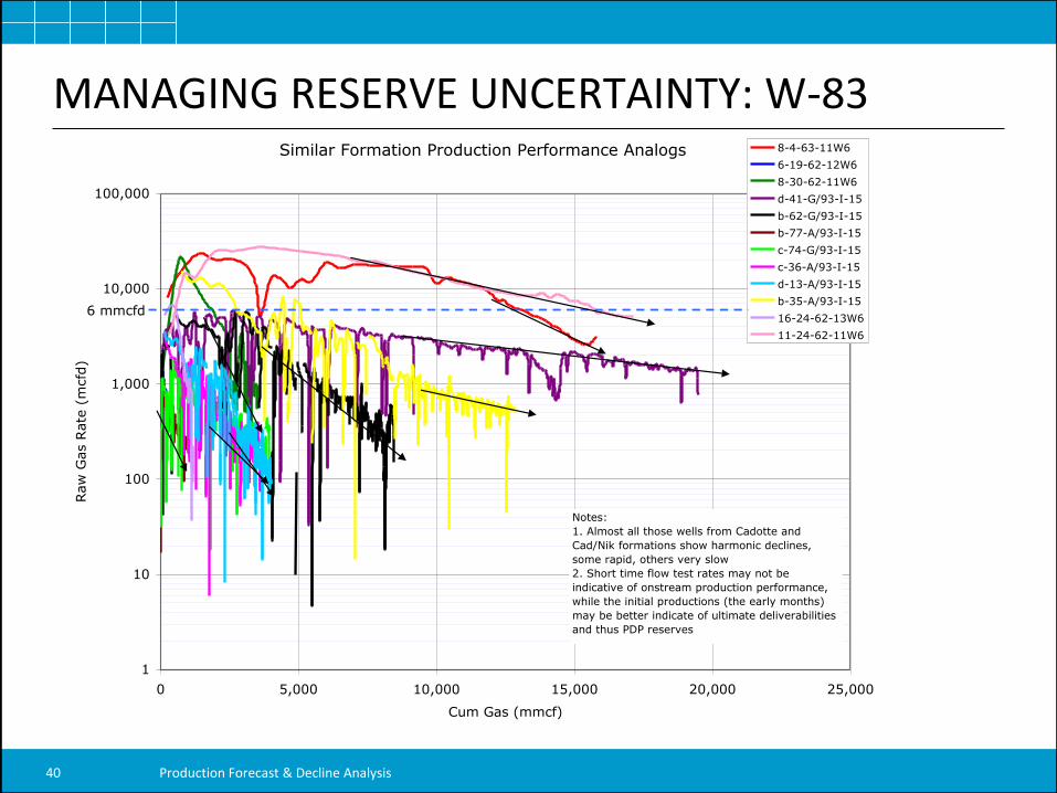
MANAGING RESERVE UNCERTAINTY: W-83 Similar Formation Production Performance Analogs
1
10
100
1,000
10,000
100,000
0 5,000 10,000 15,000 20,000 25,000
Cum Gas (mmcf)
Raw
Gas R
ate
(m
cfd
)
8-4-63-11W6
6-19-62-12W6
8-30-62-11W6
d-41-G/93-I-15
b-62-G/93-I-15
b-77-A/93-I-15
c-74-G/93-I-15
c-36-A/93-I-15
d-13-A/93-I-15
b-35-A/93-I-15
16-24-62-13W6
11-24-62-11W6
6 mmcfd
Notes:
1. Almost all those wells from Cadotte and
Cad/Nik formations show harmonic declines,
some rapid, others very slow
2. Short time flow test rates may not be
indicative of onstream production performance,
while the initial productions (the early months)
may be better indicate of ultimate deliverabilities
and thus PDP reserves
Production Forecast & Decline Analysis 40
MANAGING RESERVE UNCERTAINTY: W-83
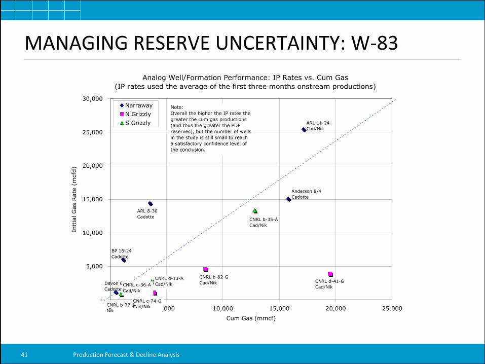
Analog Well/Formation Performance: IP Rates vs. Cum Gas
(IP rates used the average of the first three months onstream productions)
-
5,000
10,000
15,000
20,000
25,000
30,000
- 5,000 10,000 15,000 20,000 25,000
Cum Gas (mmcf)
Initia
l G
as R
ate
(m
cfd
)
Narraway
N Grizzly
S Grizzly
ARL 8-30
Cadotte
ARL 11-24
Cad/Nik
BP 16-24
Cadotte
Devon 6-19
Cadotte
CNRL c-74-G
Cad/Nik
CNRL b-82-G
Cad/Nik CNRL d-41-G
Cad/Nik
Anderson 8-4
Cadotte
CNRL b-35-A
Cad/Nik
CNRL b-77-A
Nik
CNRL d-13-A
Cad/NikCNRL c-36-A
Cad/Nik
Note:
Overall the higher the IP rates the
greater the cum gas productions
(and thus the greater the PDP
reserves), but the number of wells
in the study is still small to reach
a satisfactory confidence level of
the conclusion.
Production Forecast & Decline Analysis 41
MANAGING RESERVE UNCERTAINTY: W-83
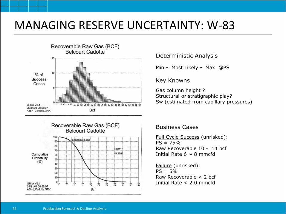
Deterministic Analysis Min ~ Most Likely ~ Max @PS
Key Knowns
Gas column height ? Structural or stratigraphic play? Sw (estimated from capillary pressures)
Business Cases
Full Cycle Success (unrisked): PS = 75% Raw Recoverable 10 ~ 14 bcf Initial Rate 6 ~ 8 mmcfd Failure (unrisked): PS = 5% Raw Recoverable < 2 bcf Initial Rate < 2.0 mmcfd
Production Forecast & Decline Analysis 42
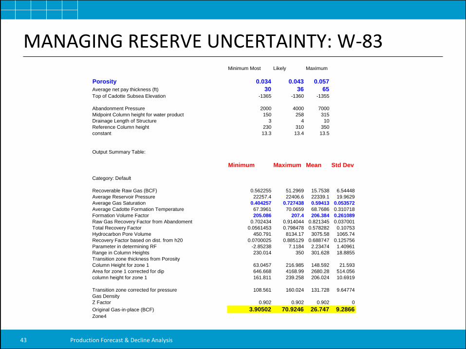
MANAGING RESERVE UNCERTAINTY: W-83 Input Summary Table:
Minimum Most Likely Maximum
Porosity 0.034 0.043 0.057
Average net pay thickness (ft) 30 36 65Top of Cadotte Subsea Elevation -1365 -1360 -1355
Abandonment Pressure 2000 4000 7000
Midpoint Column height for water product 150 258 315
Drainage Length of Structure 3 4 10
Reference Column height 230 310 350
constant 13.3 13.4 13.5
Output Summary Table:
Minimum Maximum Mean Std Dev
Category: Default
Recoverable Raw Gas (BCF) 0.562255 51.2969 15.7538 6.54448
Average Reservoir Pressure 22257.4 22406.6 22339.1 19.9629
Average Gas Saturation 0.404257 0.727438 0.59413 0.053572
Average Cadotte Formation Temperature 67.3961 70.0659 68.7686 0.310718
Formation Volume Factor 205.086 207.4 206.384 0.261089
Raw Gas Recovery Factor from Abandoment 0.702434 0.914044 0.821345 0.037001
Total Recovery Factor 0.0561453 0.798478 0.578282 0.10753
Hydrocarbon Pore Volume 450.791 8134.17 3075.58 1065.74
Recovery Factor based on dist. from h20 0.0700025 0.885129 0.688747 0.125756
Parameter in determining RF -2.85238 7.1184 2.23474 1.40961
Range in Column Heights 230.014 350 301.628 18.8855
Transition zone thickness from Porosity
Column Height for zone 1 63.0457 216.985 148.592 21.593
Area for zone 1 corrected for dip 646.668 4168.99 2680.28 514.056
column height for zone 1 161.811 239.258 206.024 10.6919
Transition zone corrected for pressure 108.561 160.024 131.728 9.64774
Gas Density
Z Factor 0.902 0.902 0.902 0
Original Gas-in-place (BCF) 3.90502 70.9246 26.747 9.2866Zone4
Production Forecast & Decline Analysis 43
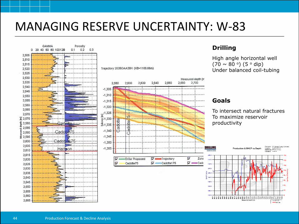
MANAGING RESERVE UNCERTAINTY: W-83
Drilling
High angle horizontal well (70 ~ 80 o) (5 o dip) Under balanced coil-tubing
Goals
To intersect natural fractures To maximize reservoir productivity
Production Forecast & Decline Analysis 44
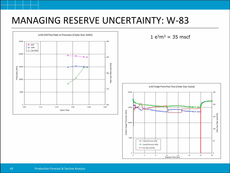
MANAGING RESERVE UNCERTAINTY: W-83 w-83 Drill Flow Rate vs Pressures (Choke Size: 54/64)
0
5000
10000
15000
20000
25000
0:00 1:12 2:24 3:36 4:48 6:00
Clock Time
Pre
ssure
s (
kP
a)
150
175
200
225
250
Raw
Gas R
ate
(e3m
3/d
)
BHP
WHP
Gas Rate
1 e3m3 = 35 mscf
Production Forecast & Decline Analysis 45
w-83 Single Point Flow Test (Choke Size Varied)
0
5000
10000
15000
20000
0 4 8 12 16 20 24 28
Elapsed Time (hrs)
Surf
ace G
auge P
ressure
s (
kP
a)
0
50
100
150
200
250
Raw
Gas R
ate
(e3m
3/d
)
Tubing Pressure (kPa)
Casing Pressures (kPa)
Gas Rate (e3m3d)
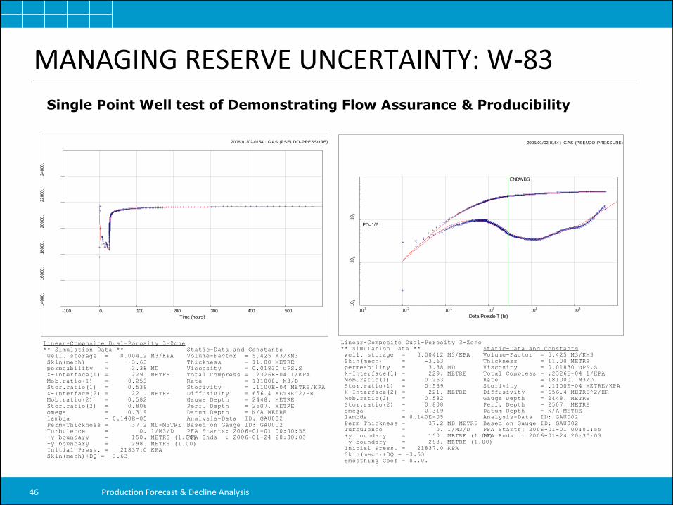
MANAGING RESERVE UNCERTAINTY: W-83
Ojay 202/a-038-H/093-I-09 Buildup
10-3 10-2 10-1 100 101 102
10
510
610
7
Delta Pseudo-T (hr)
DP
& D
ER
IVA
TIV
E (
KP
A2
/PA
S/M
3/D
)
ENDWBS
PD=1/2
2006/01/02-0154 : GAS (PSEUDO-PRESSURE)
Linear-Composite Dual-Porosity 3-Zone
** Simulation Data **
well. storage = 0.00412 M3/KPA
Skin(mech) = -3.63
permeability = 3.38 MD
X-Interface(1) = 229. METRE
Mob.ratio(1) = 0.253
Stor.ratio(1) = 0.539
X-Interface(2) = 221. METRE
Mob.ratio(2) = 0.582
Stor.ratio(2) = 0.808
omega = 0.319
lambda = 0.140E-05
Perm-Thickness = 37.2 MD-METRE
Turbulence = 0. 1/M3/D
+y boundary = 150. METRE (1.00)
-y boundary = 298. METRE (1.00)
Initial Press. = 21837.0 KPA
Skin(mech)+DQ = -3.63
Smoothing Coef = 0.,0.
Static-Data and Constants
Volume-Factor = 5.425 M3/KM3
Thickness = 11.00 METRE
Viscosity = 0.01830 uPS.S
Total Compress = .2326E-04 1/KPA
Rate = 181000. M3/D
Storivity = .1100E-04 METRE/KPA
Diffusivity = 656.4 METRE^2/HR
Gauge Depth = 2448. METRE
Perf. Depth = 2507. METRE
Datum Depth = N/A METRE
Analysis-Data ID: GAU002
Based on Gauge ID: GAU002
PFA Starts: 2006-01-01 00:00:55
PFA Ends : 2006-01-24 20:30:03
Ojay 202/a-038-H/093-I-09 Buildup
-100. 0. 100. 200. 300. 400. 500.
14000.
16000.
18000.
20000.
22000.
24000.
Time (hours)
pre
ssu
res
(KP
A)
2006/01/02-0154 : GAS (PSEUDO-PRESSURE)
Linear-Composite Dual-Porosity 3-Zone
** Simulation Data **
well. storage = 0.00412 M3/KPA
Skin(mech) = -3.63
permeability = 3.38 MD
X-Interface(1) = 229. METRE
Mob.ratio(1) = 0.253
Stor.ratio(1) = 0.539
X-Interface(2) = 221. METRE
Mob.ratio(2) = 0.582
Stor.ratio(2) = 0.808
omega = 0.319
lambda = 0.140E-05
Perm-Thickness = 37.2 MD-METRE
Turbulence = 0. 1/M3/D
+y boundary = 150. METRE (1.00)
-y boundary = 298. METRE (1.00)
Initial Press. = 21837.0 KPA
Skin(mech)+DQ = -3.63
Static-Data and Constants
Volume-Factor = 5.425 M3/KM3
Thickness = 11.00 METRE
Viscosity = 0.01830 uPS.S
Total Compress = .2326E-04 1/KPA
Rate = 181000. M3/D
Storivity = .1100E-04 METRE/KPA
Diffusivity = 656.4 METRE^2/HR
Gauge Depth = 2448. METRE
Perf. Depth = 2507. METRE
Datum Depth = N/A METRE
Analysis-Data ID: GAU002
Based on Gauge ID: GAU002
PFA Starts: 2006-01-01 00:00:55
PFA Ends : 2006-01-24 20:30:03
Single Point Well test of Demonstrating Flow Assurance & Producibility
Production Forecast & Decline Analysis 46
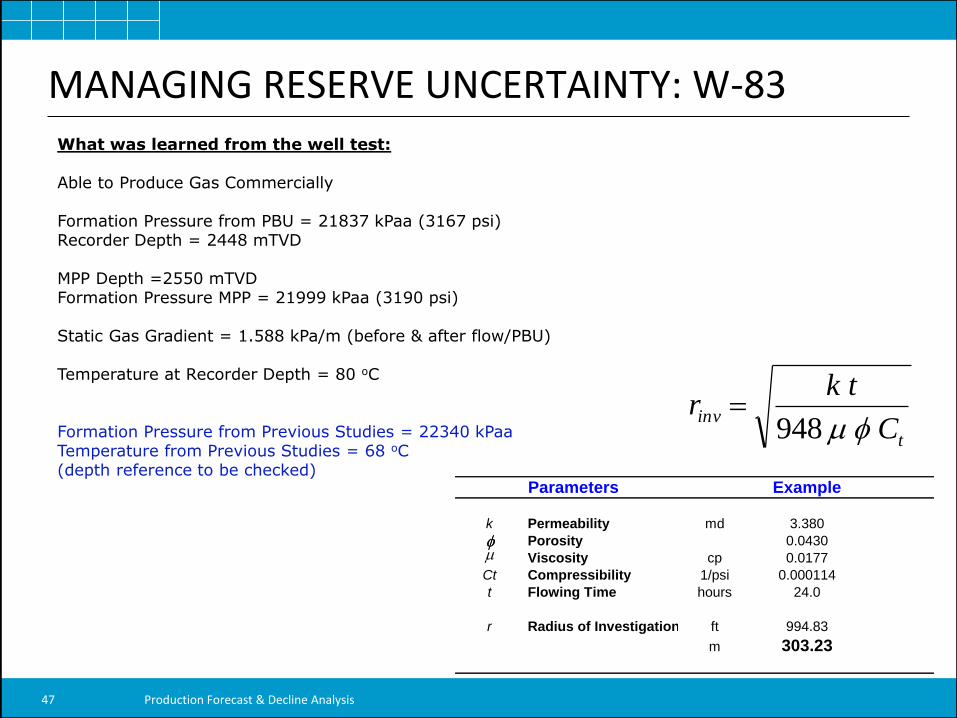
MANAGING RESERVE UNCERTAINTY: W-83 What was learned from the well test: Able to Produce Gas Commercially Formation Pressure from PBU = 21837 kPaa (3167 psi) Recorder Depth = 2448 mTVD MPP Depth =2550 mTVD Formation Pressure MPP = 21999 kPaa (3190 psi) Static Gas Gradient = 1.588 kPa/m (before & after flow/PBU) Temperature at Recorder Depth = 80 oC Formation Pressure from Previous Studies = 22340 kPaa Temperature from Previous Studies = 68 oC (depth reference to be checked)
t
invC
tkr
948
Parameters Example
k Permeability md 3.380
Porosity 0.0430
Viscosity cp 0.0177
Ct Compressibility 1/psi 0.000114
t Flowing Time hours 24.0
r Radius of Investigation ft 994.83
m 303.23
Production Forecast & Decline Analysis 47
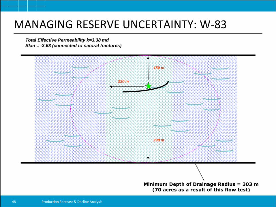
MANAGING RESERVE UNCERTAINTY: W-83 Total Effective Permeability k=3.38 md
Skin = -3.63 (connected to natural fractures)
Minimum Depth of Drainage Radius = 303 m (70 acres as a result of this flow test)
298 m
150 m
220 m
Production Forecast & Decline Analysis 48
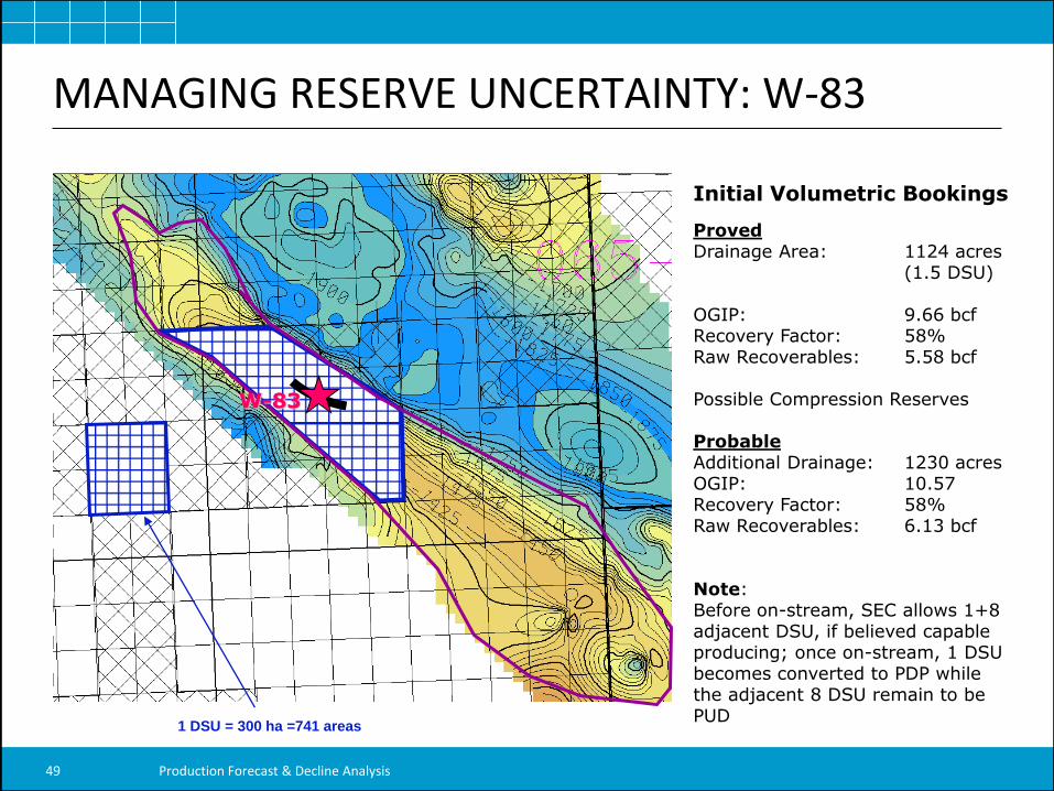
Initial Volumetric Bookings
Proved Drainage Area: 1124 acres (1.5 DSU) OGIP: 9.66 bcf Recovery Factor: 58% Raw Recoverables: 5.58 bcf Possible Compression Reserves Probable Additional Drainage: 1230 acres OGIP: 10.57 Recovery Factor: 58% Raw Recoverables: 6.13 bcf Note: Before on-stream, SEC allows 1+8 adjacent DSU, if believed capable producing; once on-stream, 1 DSU becomes converted to PDP while the adjacent 8 DSU remain to be PUD
W-83
1 DSU = 300 ha =741 areas
MANAGING RESERVE UNCERTAINTY: W-83
Production Forecast & Decline Analysis 49
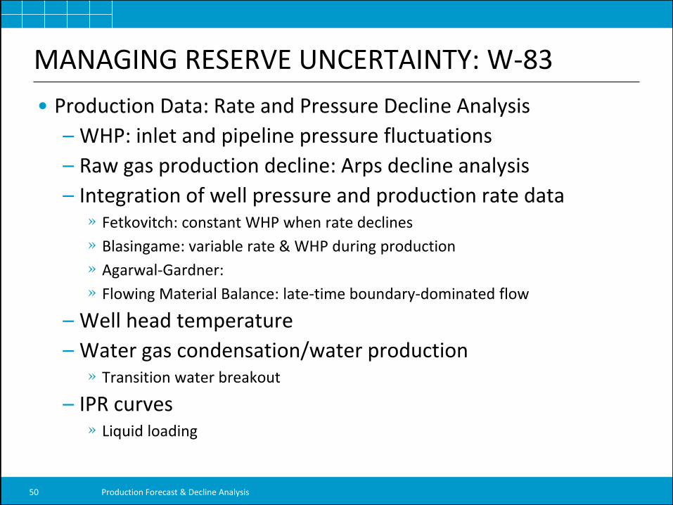
• Production Data: Rate and Pressure Decline Analysis
– WHP: inlet and pipeline pressure fluctuations
– Raw gas production decline: Arps decline analysis
– Integration of well pressure and production rate data » Fetkovitch: constant WHP when rate declines
» Blasingame: variable rate & WHP during production
» Agarwal-Gardner:
» Flowing Material Balance: late-time boundary-dominated flow
– Well head temperature
– Water gas condensation/water production » Transition water breakout
– IPR curves » Liquid loading
MANAGING RESERVE UNCERTAINTY: W-83
Production Forecast & Decline Analysis 50
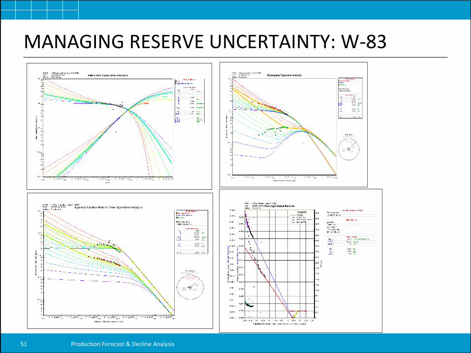
MANAGING RESERVE UNCERTAINTY: W-83
Production Forecast & Decline Analysis 51
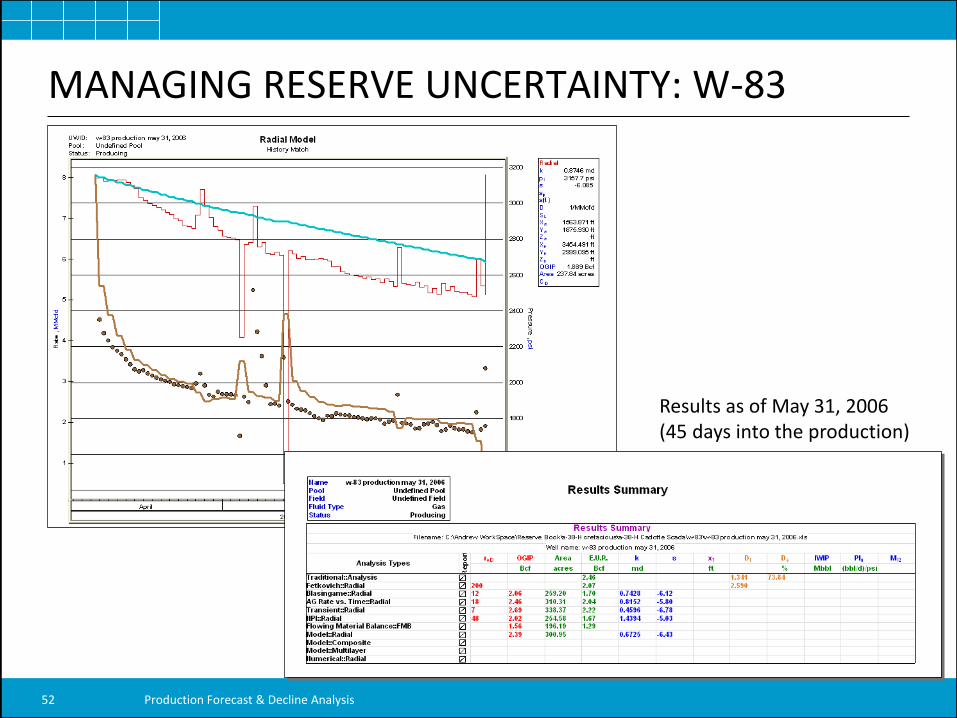
MANAGING RESERVE UNCERTAINTY: W-83
Production Forecast & Decline Analysis 52
Results as of May 31, 2006 (45 days into the production)
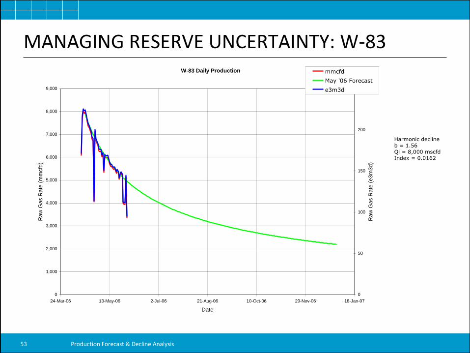
Harmonic decline b = 1.56 Qi = 8,000 mscfd Index = 0.0162
MANAGING RESERVE UNCERTAINTY: W-83 W-83 Daily Production
0
1,000
2,000
3,000
4,000
5,000
6,000
7,000
8,000
9,000
24-Mar-06 13-May-06 2-Jul-06 21-Aug-06 10-Oct-06 29-Nov-06 18-Jan-07
Date
Raw
Gas R
ate
(m
mcfd
)
0
50
100
150
200
250
Raw
Gas R
ate
(e3m
3d)
mmcfd
May '06 Forecast
e3m3d
Production Forecast & Decline Analysis 53
MANAGING RESERVE UNCERTAINTY: W-83
• Production Rate Decline Related to……
– Reservoir Production mechanism: natural depletion? water drive?
– Wellbore problems: liquid loading, multiple phase, non-hydrocarbon?
– Reservoir characteristics:
» Smaller reservoir tank? Compartmentalized?
» Misinterpreted reservoir parameters (net pay, transition)?
» Low matrix permeability? Lack of natural fracture networks/connectivity?
• “Proved” Reserve Calibrated and Re-Filed ……
– How much producible/economic reserve this well can “see”?
– New reserve/resource estimate and new forecast
– Well workover/facility options?
» Tubing size change? Acidizing/fracturing? Compressor?
Production Forecast & Decline Analysis 54
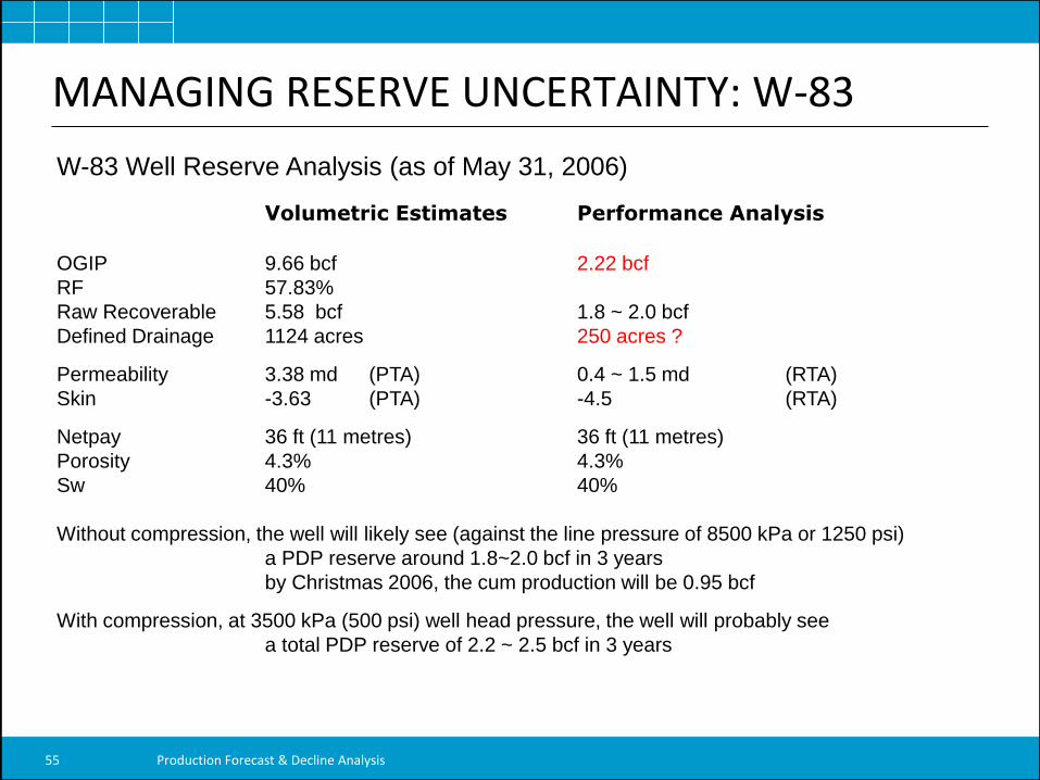
W-83 Well Reserve Analysis (as of May 31, 2006)
Volumetric Estimates Performance Analysis
OGIP 9.66 bcf 2.22 bcf
RF 57.83%
Raw Recoverable 5.58 bcf 1.8 ~ 2.0 bcf
Defined Drainage 1124 acres 250 acres ?
Permeability 3.38 md (PTA) 0.4 ~ 1.5 md (RTA)
Skin -3.63 (PTA) -4.5 (RTA)
Netpay 36 ft (11 metres) 36 ft (11 metres)
Porosity 4.3% 4.3%
Sw 40% 40%
Without compression, the well will likely see (against the line pressure of 8500 kPa or 1250 psi)
a PDP reserve around 1.8~2.0 bcf in 3 years
by Christmas 2006, the cum production will be 0.95 bcf
With compression, at 3500 kPa (500 psi) well head pressure, the well will probably see
a total PDP reserve of 2.2 ~ 2.5 bcf in 3 years
MANAGING RESERVE UNCERTAINTY: W-83
Production Forecast & Decline Analysis 55
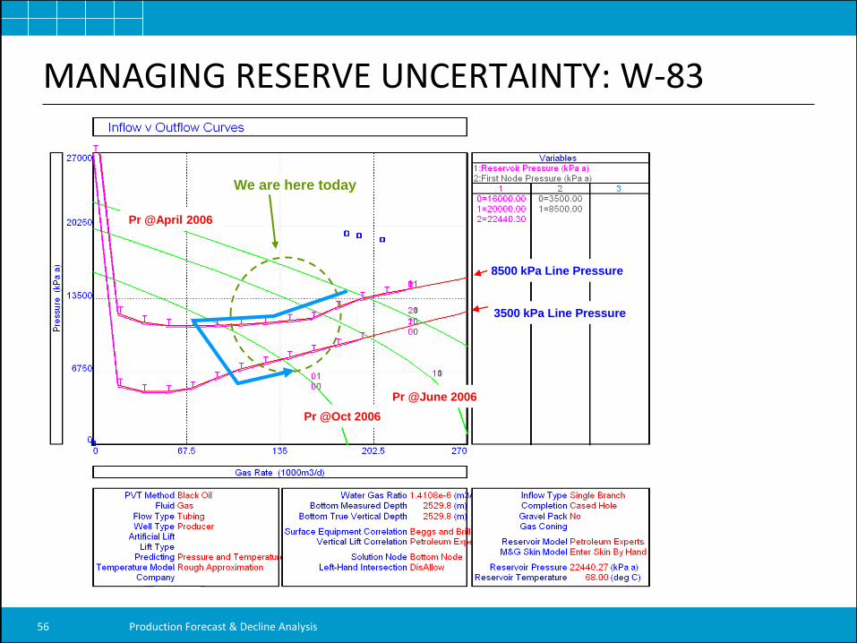
MANAGING RESERVE UNCERTAINTY: W-83
Pr @June 2006
Pr @Oct 2006
8500 kPa Line Pressure
3500 kPa Line Pressure
We are here today
Pr @April 2006
Production Forecast & Decline Analysis 56
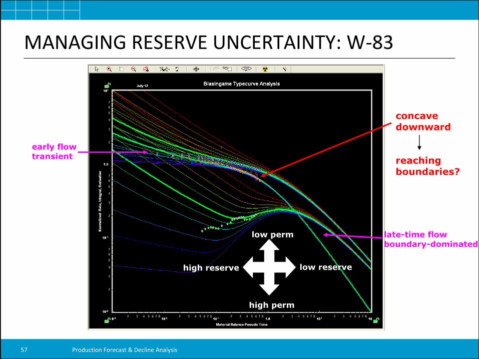
concave downward reaching boundaries?
high reserve low reserve
high perm
low perm
early flow transient
late-time flow boundary-dominated
MANAGING RESERVE UNCERTAINTY: W-83
Production Forecast & Decline Analysis 57
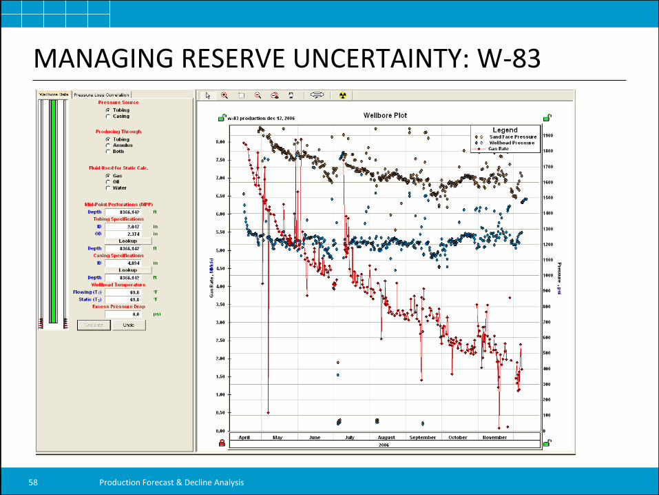
MANAGING RESERVE UNCERTAINTY: W-83
Production Forecast & Decline Analysis 58
MANAGING RESERVE UNCERTAINTY: W-83
Production Forecast & Decline Analysis 59
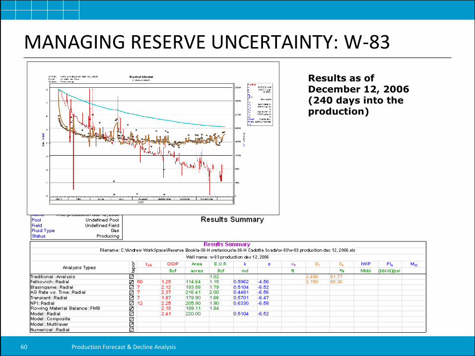
MANAGING RESERVE UNCERTAINTY: W-83
Results as of December 12, 2006 (240 days into the production)
Production Forecast & Decline Analysis 60
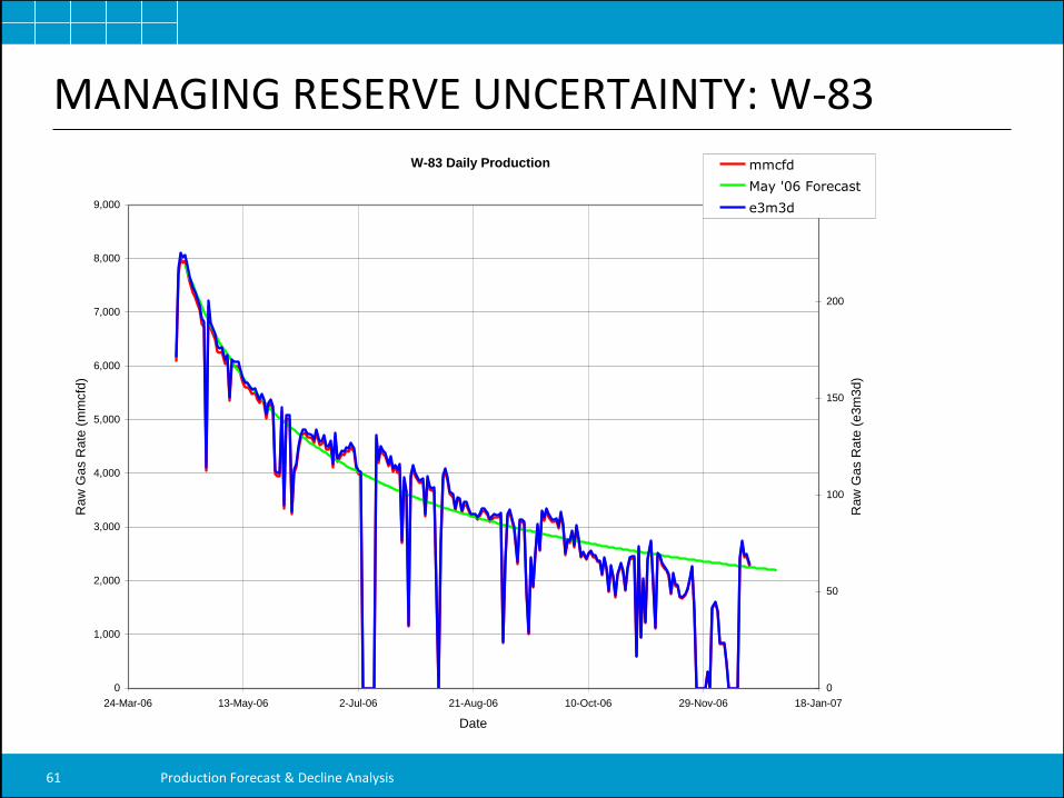
W-83 Daily Production
0
1,000
2,000
3,000
4,000
5,000
6,000
7,000
8,000
9,000
24-Mar-06 13-May-06 2-Jul-06 21-Aug-06 10-Oct-06 29-Nov-06 18-Jan-07
Date
Ra
w G
as R
ate
(m
mcfd
)
0
50
100
150
200
250
Ra
w G
as R
ate
(e
3m
3d
)
mmcfd
May '06 Forecast
e3m3d
MANAGING RESERVE UNCERTAINTY: W-83
Production Forecast & Decline Analysis 61
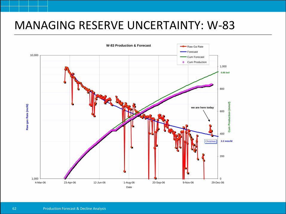
W-83 Production & Forecast
1,000
10,000
4-Mar-06 23-Apr-06 12-Jun-06 1-Aug-06 20-Sep-06 9-Nov-06 29-Dec-06
Date
Raw
ga
s R
ate
(m
cfd
)
0
200
400
600
800
1,000
Cu
m P
rod
uc
tio
n (
mm
cf)
Raw Ga Rate
Forecast
Cum Forecast
Cum Production
Christmas
0.95 bcf
2.2 mmcfd
we are here today
MANAGING RESERVE UNCERTAINTY: W-83
Production Forecast & Decline Analysis 62
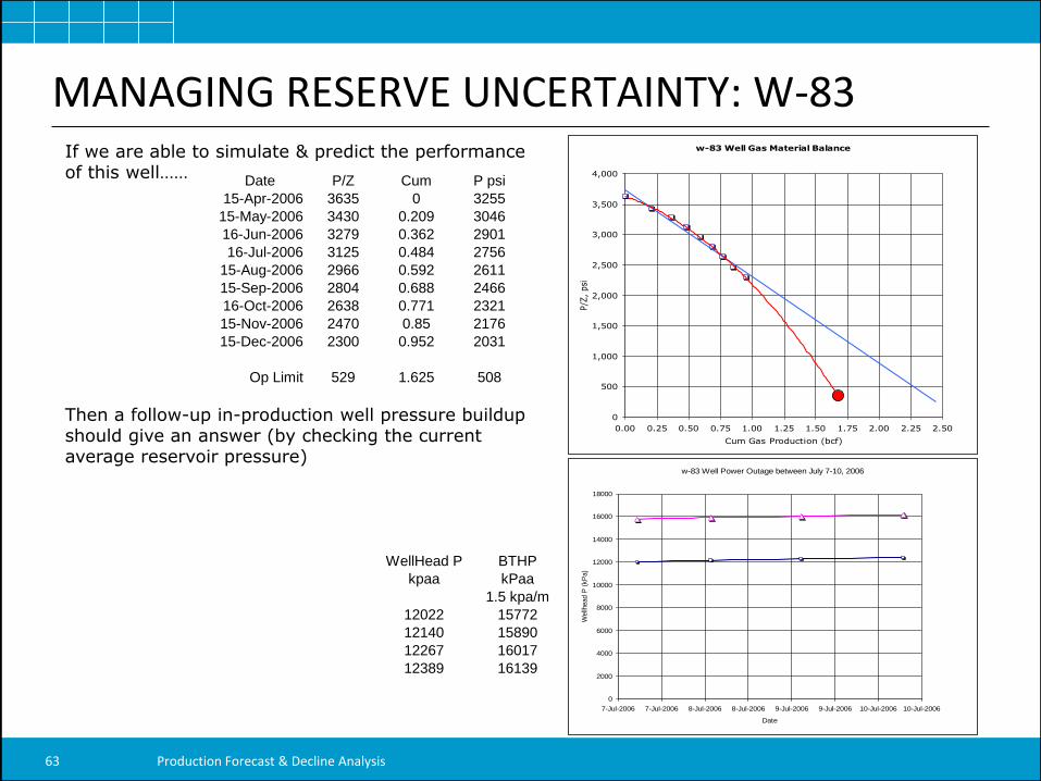
MANAGING RESERVE UNCERTAINTY: W-83 w-83 Well Gas Material Balance
0
500
1,000
1,500
2,000
2,500
3,000
3,500
4,000
0.00 0.25 0.50 0.75 1.00 1.25 1.50 1.75 2.00 2.25 2.50
Cum Gas Production (bcf)
P/Z
, psi
Date P/Z Cum P psi
15-Apr-2006 3635 0 3255
15-May-2006 3430 0.209 3046
16-Jun-2006 3279 0.362 2901
16-Jul-2006 3125 0.484 2756
15-Aug-2006 2966 0.592 2611
15-Sep-2006 2804 0.688 2466
16-Oct-2006 2638 0.771 2321
15-Nov-2006 2470 0.85 2176
15-Dec-2006 2300 0.952 2031
Op Limit 529 1.625 508
If we are able to simulate & predict the performance of this well……
Then a follow-up in-production well pressure buildup should give an answer (by checking the current average reservoir pressure)
w-83 Well Power Outage between July 7-10, 2006
0
2000
4000
6000
8000
10000
12000
14000
16000
18000
7-Jul-2006 7-Jul-2006 8-Jul-2006 8-Jul-2006 9-Jul-2006 9-Jul-2006 10-Jul-2006 10-Jul-2006
Date
Wellh
ead P
(kP
a)
WellHead P BTHP
kpaa kPaa
1.5 kpa/m
12022 15772
12140 15890
12267 16017
12389 16139
Production Forecast & Decline Analysis 63
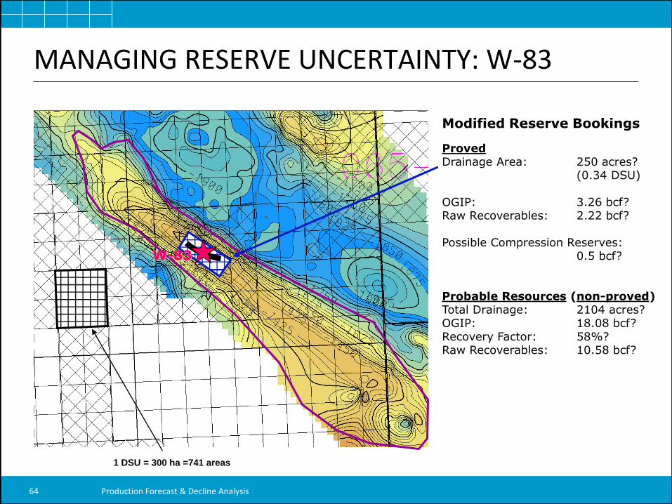
Modified Reserve Bookings
Proved Drainage Area: 250 acres? (0.34 DSU) OGIP: 3.26 bcf? Raw Recoverables: 2.22 bcf? Possible Compression Reserves: 0.5 bcf? Probable Resources (non-proved) Total Drainage: 2104 acres? OGIP: 18.08 bcf? Recovery Factor: 58%? Raw Recoverables: 10.58 bcf?
1 DSU = 300 ha =741 areas
W-83
MANAGING RESERVE UNCERTAINTY: W-83
Production Forecast & Decline Analysis 64
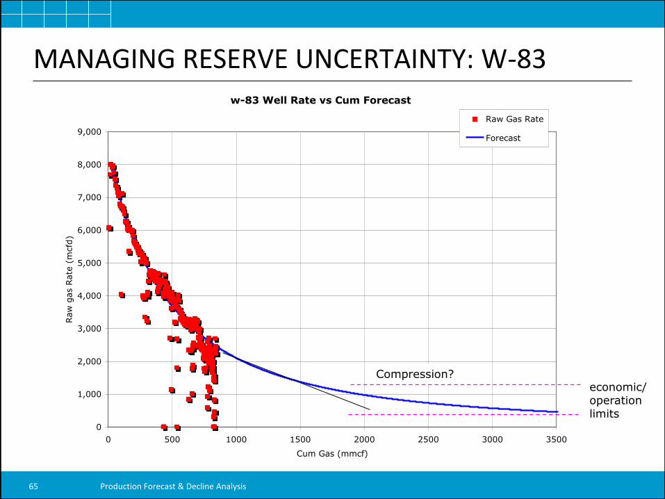
MANAGING RESERVE UNCERTAINTY: W-83 w-83 Well Rate vs Cum Forecast
0
1,000
2,000
3,000
4,000
5,000
6,000
7,000
8,000
9,000
0 500 1000 1500 2000 2500 3000 3500
Cum Gas (mmcf)
Raw
gas R
ate
(m
cfd
)
Raw Gas Rate
Forecast
economic/ operation limits
Compression?
Production Forecast & Decline Analysis 65
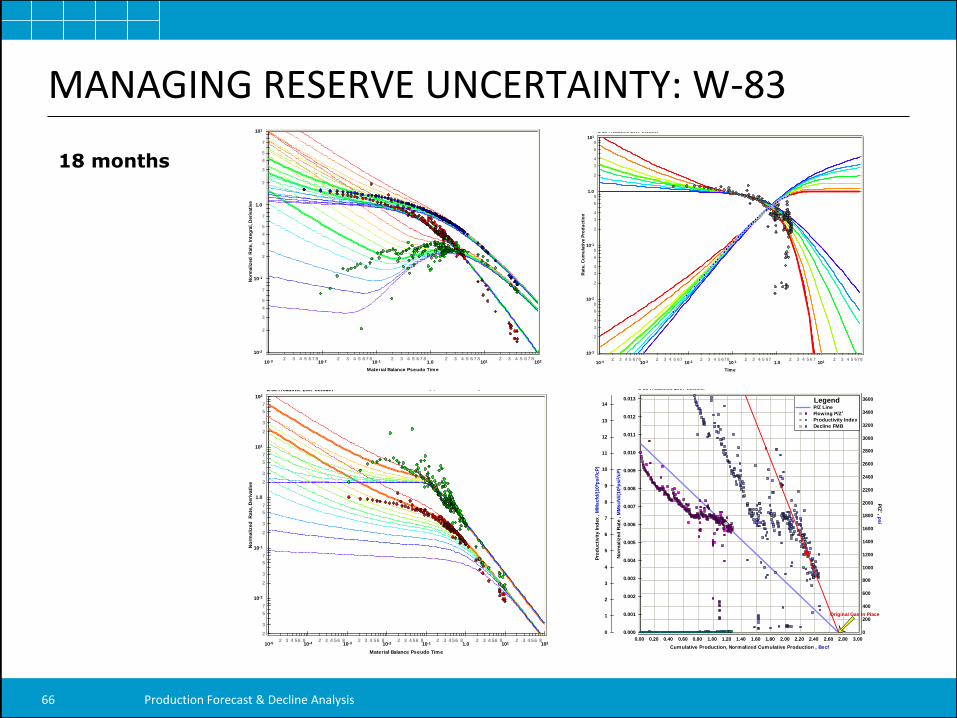
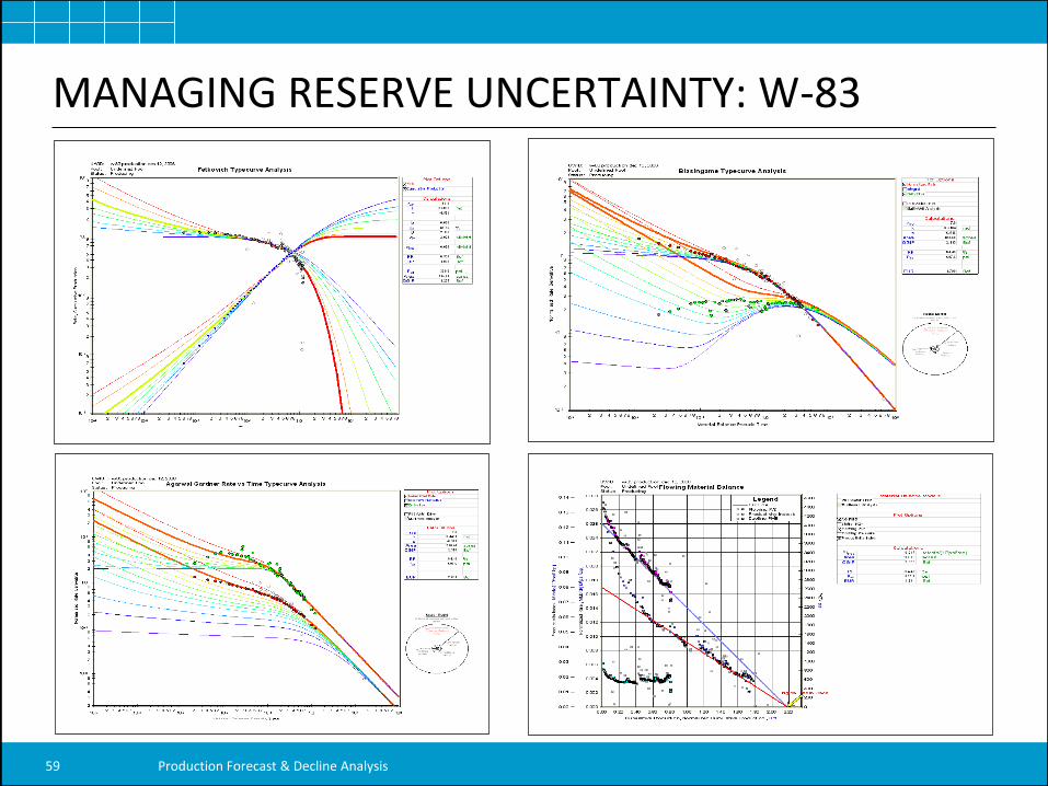
MANAGING RESERVE UNCERTAINTY: W-83
18 months
10-3 10-2 10-1 1.0 101 1022 3 4 5 6 7 8 2 3 4 5 6 7 8 2 3 4 5 6 7 8 2 3 4 5 6 7 8 2 3 4 5 6 7 8
Material Balance Pseudo Time
10-2
10-1
1.0
101
2
3
4
5
7
2
3
4
5
7
2
3
4
5
7
No
rmalized
R
ate
, In
teg
ral, D
eri
vati
ve
Blasingame Typecurve Analysisa-38-H cadotte 2007 october
10-4 10-3 10-2 10-1 1.0 1012 3 4 5 678 2 3 4 5 67 2 3 4 5 678 2 3 4 5 67 2 3 4 5 6 7 2 3 4 5 678
Time
10-3
10-2
10-1
1.0
101
2
3
4
6
8
2
3
4
6
8
2
3
4
6
8
2
3
4
6
8
Rate
, C
um
ula
tive P
rod
ucti
on
Fetkovich Typecurve Analysisa-38-H cadotte 2007 october
10-5 10-4 10-3 10-2 10-1 1.0 101 1022 3 4 56 8 2 3 4 56 8 2 3 4 56 8 2 3 4 56 8 2 3 4 56 8 2 3 4 56 8 2 3 4 56 8
Material Balance Pseudo Time
10-2
10-1
1.0
101
102
2
3
5
7
2
3
5
7
2
3
5
7
2
3
5
7
2
3
5
7
No
rmalized
R
ate
, D
eri
vati
ve
Agarwal Gardner Rate vs Time Typecurve Analysisa-38-H cadotte 2007 october
0.00 0.20 0.40 0.60 0.80 1.00 1.20 1.40 1.60 1.80 2.00 2.20 2.40 2.60 2.80 3.00
Cumulative Production, Normalized Cumulative Production , Bscf
0
1
2
3
4
5
6
7
8
9
10
11
12
13
14
Pro
du
cti
vit
y In
dex , M
Mscfd
/(10
6p
si2
/cP
)
0.000
0.001
0.002
0.003
0.004
0.005
0.006
0.007
0.008
0.009
0.010
0.011
0.012
0.013
No
rmalized
Rate
, M
Mscfd
/(10
6p
si2
/cP
)
0
200
400
600
800
1000
1200
1400
1600
1800
2000
2200
2400
2600
2800
3000
3200
3400
3600
P/Z
* , psi
Flowing Material Balancea-38-H cadotte 2007 october
Original Gas In Place
LegendP/Z Line
Flowing P/Z*
Productivity Index
Decline FMB
Production Forecast & Decline Analysis 66