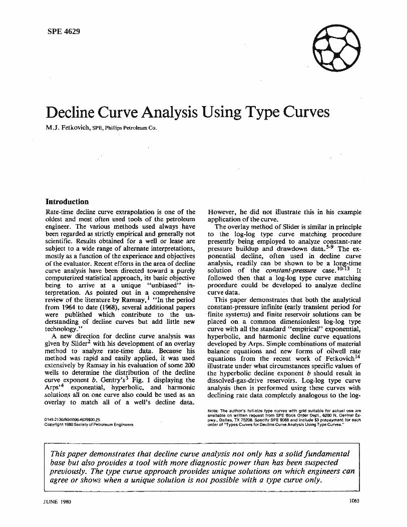
SPE 4629

Decline Curve Analysis Using Type Curves M.J. Fetkovich, SPE, Phillips Petroleum Co.

Introduction Rate-time decline curve extrapolation· is one of the oldest and most often used tools of the petroleum engineer. The various methods used always have been regarded as strictly empirical and generally not scientific. Results obtained for a well or lease are subject to a wide range of alternate interpretations, mostly as a function of the experience and objectives of the evaluator. Recent efforts in the area of decline curve analysis have been directed toward a purely computerized statistical approach, its basic objective being to arrive at a unique "unbiased" in­terpretation. As pointed out in a comprehensive review of the literature by Ramsay,l "In the period from 1964 to date (1968), several additional papers were published which contribute to the un­derstanding of decline curves but add little new technology. "

A new direction for decline curve analysis was given by Slider2 with his development of an overlay method to analyze rate-time data. Because his method was rapid and easily applied, it was used extensively by Ramsay in his evaluation of some 200 wells to determine the distribution of the decline curve exponent b. Gentry's3 Fig. 1 displaying the Arps,4 exponential, hyperbolic, and harmonic solution,s all on one curve also could be used as an overlay to match all of a well's decline data.

0149·2136180/0006-4629$00.25 Copyright 1980 SOCiety of Petroleum Engineers

However, he did not illustrate this in his example application of the curve.

The overlay method of Slider is similar in principle to the log-log type curve matching procedure presently being employed to analyze constant-rate pressure buildup and drawdown data. 5-9 The ex­ponential decline, often used in decline curve analysis, readily can be shown to be a lon,-time solution of the constant-pressure case. 10- 3 It followed then that a log-log type curve matching procedure could be developed to analyze decline curve data.

This paper demonstrates that both the analytical constant-pressure infinite (early transient period for finite systems) and finite reservoir solutions can be placed on a common dimensionless log-log type curve with all the standard "empirical" exponential, hyperbolic, and harmonic decline curve equations developed by Arps. Simple combinations of material balance equations and new forms of oilwell rate equations from the recent work of Fetkovich 14 illustrate under what circumstances specific values of the hyperbolic decline exponent b should result in dissolved-gas-drive reservoirs. Log-log type curve analysis then is performed using these curves with declining rate data completely analogous to the log-

Note: The author's full·size type curves with grid suitable for actual use are available on written request from SPE Book Order Dept., 6200 N. Central Ex· pwy., Dallas, TX 75206. Specify SPE 9086 and include $3 prepayment for each order of "Types Curves for Decline Curve Analysis Using Type Curves."

This paper demonstrates that decline curve analysis not only has a solid fundamental base but also provides a tool with more diagnostic power than has been suspected previously. The type curve approach provides unique solutions on which engineers can agree or shows when a unique solution is not possible with a type curve only. .

JUNE 1980 1065

t RATE _ nMf EOVATIQNS

I~,* .-' ,'D">' ~ '.D,'J'

.!ill . ----1-;f'~b.O "i eDil -_._- - -

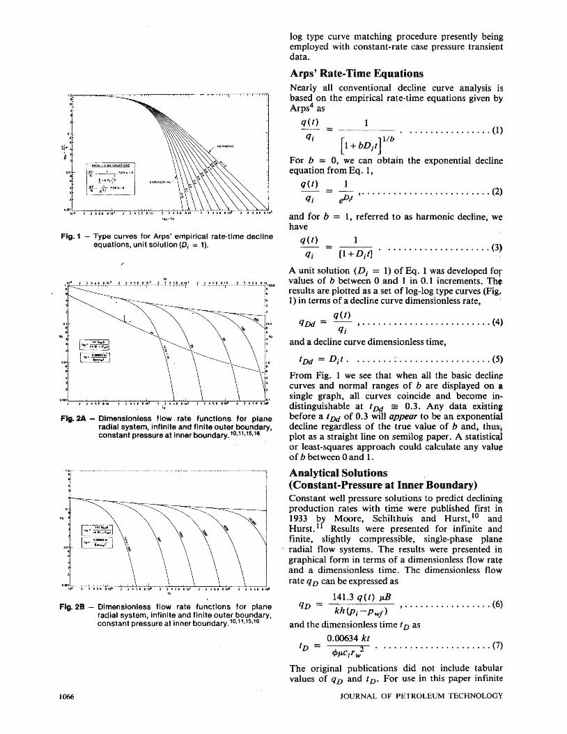
Fig. 1 - Type curves for Arps' empirical rate-time decline equations, unit solution (0; = 1).

.. ~'iS",----:-' -c:-'-C:-'+''';'''';'''TMt,,---' -:''--.;-' :;...:' 'C<-'...;." T-'~'-";'" -c:-'--r' ..;..:' ';.,..;';.;;:'~-'--:',---"-' .;...c' ,~,.-"-. r'·O---:.'-,'=-.:'c=.'.:.,.' ~. 1':100_ ,

0.' . ,

0 .• ' .

Fig. 2A - Dimensionless flow · rate functions for plane radial system, infinite and finite outer boundary, constant pressure at inner boundary.l0.ll,15,18

' .:r-~~-------~~~-------'

0J[~~~~::----==----J

"·1

Fig. 28 - Dimensionless flow rate functions for plane radial system, infinite and finite outer boundary, constant pressure at inner boundary.l0,11,15,16

1066

log type curve matching procedure presently being employed with constant-rate case pressure transient data.

Arps' Rate-Time Equations Nearly all conventional decline curve analysis is based on the empirical rate-time equations given by Arps4 as

q(t) = ---- ................. (1)

q; [1 + bD;tflb

For b = 0, we can obtain the exponential dedine equation from Eq. 1,

q(t) 1 -=-, .......................... (2)

q; eDit

and for b = I, referred to as harmonic decline, we have

q(t)

qj = . ....................... (3)

[1 +D;t]

A unit solution (D; = 1) of Eq. 1 was developed for values of b between 0 and 1 in 0.1 increments. Th~ results are plotted as a set of log-log type curves (Fig I 1) in terms of a decline curve dimensionless rate,

q(t) qDd = - , ......................... (4)

qj

and a decline curve dimensionless time,

t Dd = D; t. . ...... : . . ................ (5)

From Fig. 1 we see that when all the basic declin~ curves and normal ranges of b are displayed on • single graph, all curves coincide and become in· distinguishable at tDd == 0.3. Any data existin$ before a tDd of 0.3 will appear to be an exponential decline regardless of the true value of b and, thus· plot as a straight line on semilog paper. A statistic;} or least-squares approach could calculate any valu~ of b between 0 and 1.

Analytical Solutions (Constant-Pressure at Inner Boundary) Constant well pressure solutions to predict declinins production rates with time were published first in 1933 b(' Moore, Schilthuis and Hurst,lO and Hurst. 1 Results were presented for infinite and finite, slightly compressible, single-phase plane radial flow systems. The results were presented in graphical form in terms of a dimensionless flow rate and a dimensionless time. The dimensionless flow rate q D can be expressed as

141.3 q(t) p.B qD = kh(p;-Pwj) , ................. (6)

and the dimensionless time t D as

0.00634 kt tD = cpp.ct

r w2 ...................... (7)

The original publications did not include tabular values of qD and tD . For use in this paper infinite

JOURNAL OF PETROLEUM TECHNOLOGY

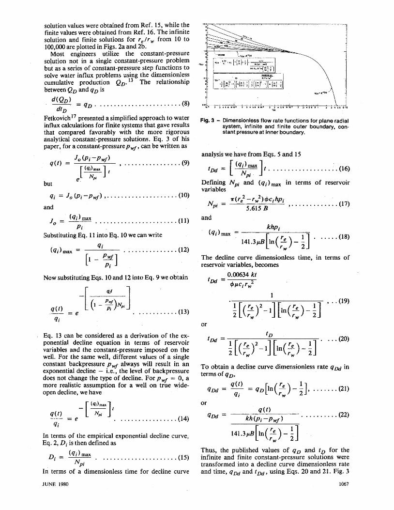
solution values were obtained from Ref. 15, while the finite values were obtained from Ref. 16. The infinite solution and finite solutions for r e/ r w from 10 to 100,000 are plotted in Figs. 2a and 2b.

Most engineers utilize the constant-pressure solution not in a single constant-pressure problem but as a series of constant-pressure step functions to solve water influx problems using the dimensionless cumulative production QD. 13 The relationship between QD and qD is

d(QD> --. = qD ' ....................... (8) dID

Fetkovich17 presented a simplified approach to water ihflux calculations for finite systems that gave results that compared favorably with the more rigorous analytical constant-pressure solutions. Eq. 3 of his paper, for a constant-pressure P wi' can be written as

10 (p;-Pwj> q (t) = • . ............. ,. (9)

[(q~max ] t but

e . PI

qi = 10 (Pi ~Pwj) , .....••.•...•....... (10)

and

10 = (qj)max ..••..•••...••...•..... (11) Pi .

Substituting Eq. 11 into Eq. 10 we can write

............... (12)

[1 - ;;] Now substituting Eqs. 10 and 12 into Eq. 9 we obtain

q(t) =e ........... (13)

Eq. 13 can be considered as a derivation of the ex­ponential decline equation in terms of reservoir variables and the constant-pressure imposed on the well. For the same well, different values of a single constant backpressure Pwj always will result in an exponential decline - i.e., the level of back pressure does not change the type of decline. For Pwj = 0, a more realistic assumption for a well on true wide­open decline, we have

q(t)

qi

[ (q;)max]

- -- t Np;

=e ...........•..•. (14)

In terms of the empirical exponential decline curve, Eq. 2, D i is then defined as

Di = (q~ ~ax . . .................... (15) pI

In terms of a dimensionless time for decline curve

JUNE 1980

'.'''". --Q'~-,-.-,-,.,,-~~...,..,.,..---~~~~~-,..,...,--~~ .

... o .

o.o:';. •.• ~, ~,-:-. ::-: .. :";.';!;; ... ,;---t,~,--;.-:-; .. ~.;-:;,,,~,~, .~,:7. ~"i;;,.'~' ~~t"'!----::-~~ ''''

Fig. 3 - ' Dimensionless flow rate functions for plane radial system, infinite and finite outer boundary, con­stant pressure at inner boundary.

analysis we have from Eqs. 5 and 15

[(qi)max]

IDd =Np; . t .. ................. (16)

Defining Np; and (qj) max in terms of reservoir variables

1f(re2 - r w2)cPCthp; Npi = 5.615 B , ............. (17)

and

[ ( r e. ) 1 .].. .... (18) 141.3p.B In- --rw 2

The decline curve dimensionless time, in terms of . reservoir variables, becomes

1 , .. (19)

or

To obtain a decline curve dimensionless rate qDd in terms of qD,

qDd = q(~l = qD[ln( re ) - ~], ....... (21) q, rw 2

or q(t)

......... (22)

141.3p.B[ln( r e ) _ ~] rw 2

Thus, the published values of qD and tD for the infinite and finite constant-pressure solutions were transformed into a decline curve dimensionless rate and time, q Dd and t Dd, using Eqs. 20 and 21. Fig. 3

1067

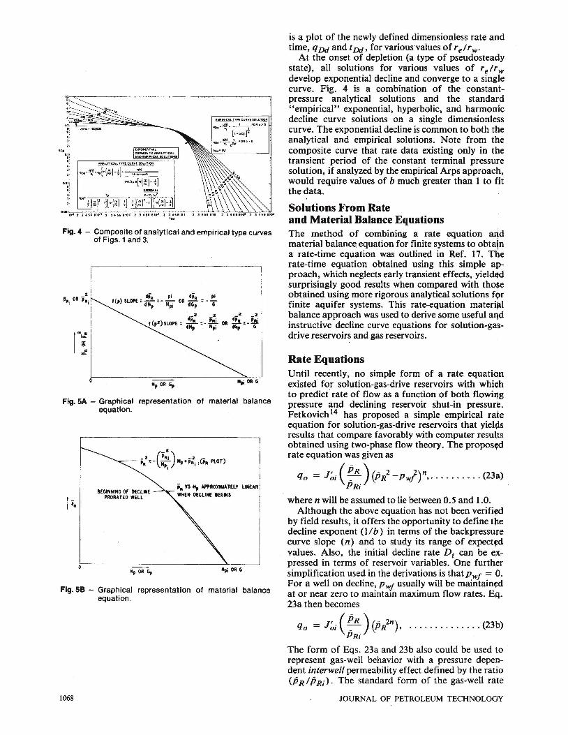
Fig. 4 - Composite of analytical and empirical type curves of Figs. 1 and 3.

IN '" I ...

!!i ..:

Np OR Gp

Fig. 5A - Graphical representation of material balance equation.

8EGINNING Of DECLINE PRORATED WEll

Hpj OR G

Fig. 58 - Graphical representation of material balance equation.

1068

is a plot of the newly defined dimensionless rate and time, qDd and t Dd' for various'values of r elr W'

At the onset of depletion (a type of pseudosteady state), all solutions for various values of relrw develop exponential decline and converge to a single curve. Fig. 4 is a combination of the constant­pressure analytical solutions and the standard "empirical" exponential, hyperbolic, and harmonic decline curve solutions on a single dimensionless curve. The exponential decline is common to both the analytical and empirical solutions. Note from the composite curve that rate data existing only in the transient period of the constant terminal pressure solution, if analyzed by the empirical Arps approach, would require values of b much greater than 1 to fit the data.

Solutions From Rate and Material Balance Equations The method of combining a rate equation and material balance equation for finite systems to obtain a rate-time equation was outlined in Ref. 17. The rate-time equation obtained using this simple a.,­proach, which neglects early transient effects, yieldl$d surprisingly good results when compared with tho$e obtained using more rigorous analytical solutions f()r finite aquifer systems. This rate-equation materi/ll balance approach was used to derive some useful alld instructive decline curve equations for solution-gas­drive reservoirs and gas reservoirs.

Rate Equations Until recently, no simple form of a rate equation existed for solution-gas-drive reservoirs with whi~h to predict' rate of flow as a function of both flowing pressure and declining reservoir shut-in pressure. Fetkovich 14 has proposed a simple empirical rate equation for solution-gas-drive reservoirs that yiel<1s results that compare favorably with computer results obtained using two-phase flow theory. The propos¢ rate equation was given as

qo = J~i(~R ) (fJi-pw!)n, .......... (23~) PRi

where n will be assumed to lie between 0.5 and 1.0. Although the above equation has not been verifi~d

by field results, it offers the opportunity to define the decline exponent (1/ b) in terms of the back pressure curve slope (n) and to study its range of expect¢<l values. Also, the initial decline rate Di can be ex­pressed in terms of reservoir variables. One further simplification used in the derivations is that Pwf = O. For a well on decline, Pw! usually will be maintained at or near zero to maintam maximum flow rates. Eq. 23a then becomes

qo = J~i (~R ) (fJin) , .............. (23b) PRi

The form of Eqs. 23a and 23b also could be used to represent gas-well behavior with a pressure depen­dent interwell permeability effect defined by the ratio (p R I fJ Ri)' The standard form of the gas-well rate

JOURNAL OF PETROLEUM TECHNOLOGY

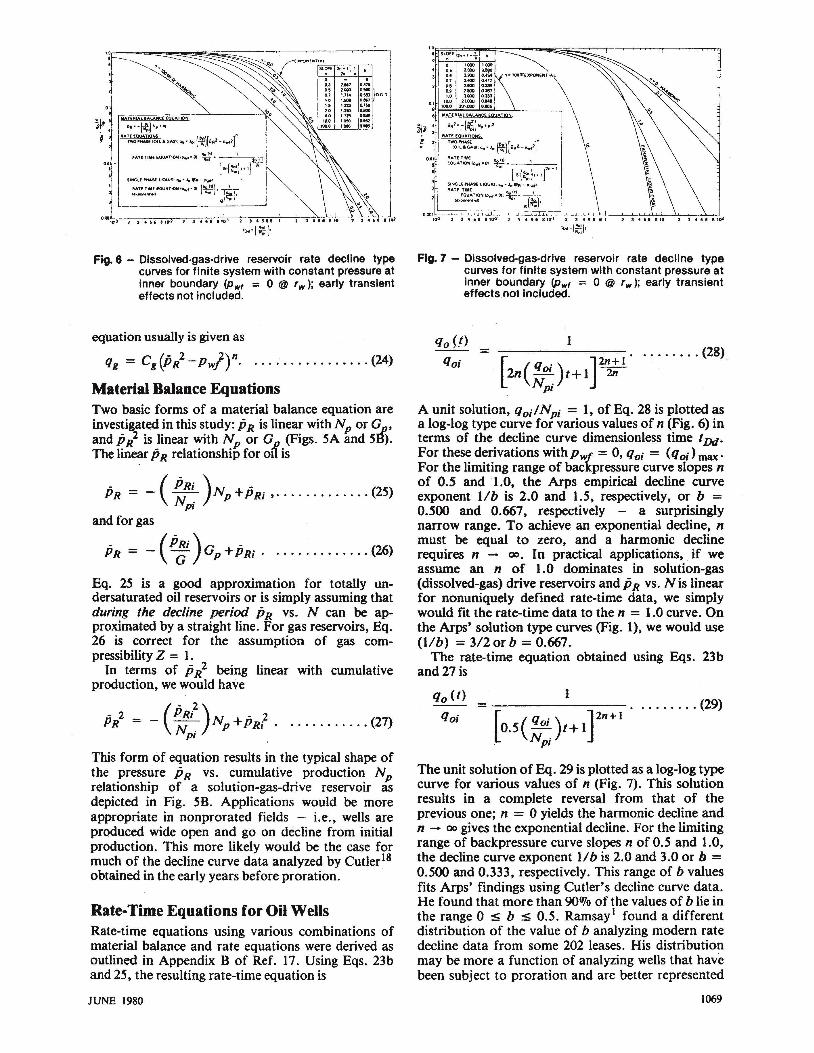
Fig. 6 - Dissolved-gas-drive reservoir rate decline type curves for finite system with constant pressure at inner boundary (Pwf = 0 @ 'w); early transient effects not included.

equation usually is given as

C {- 2 2)n qg = gVJR -Pwj . ................ (24)

Material Balance Equations Two basic forms of a material balance equation are investigated in this study: P R is linear with Np or f:!p, and pi is linear with Np or Gp (Figs. 5A and 58). The linear PR relationship for 011 is

PR = - ( ~R~ )Np +PRi , ............. (25) PI

and for gas

PR = - (p~; ) Gp +PRi. . ............ (26)

Eq. 25 is a good approximation for totally un­dersaturated oil reservoirs or is simply assuming that during the decline period P R vs. N can be ap­proximated by a straight line. For gas reservoirs, Eq. 26 is correct for the assumption of gas com­pressibility Z = 1.

In terms of pi being linear with cumulative production, we would have

- 2 _ (fiR?) N - 2 P R - - N. p + P Ri . . .......... (27) pi ,

This form of equation results in the typical shape of the pressure PR vs. cumulative production Np relationship of a solution-gas-drive reservoir as depicted in Fig. 5B. Applications would be more appropriate in nonprorated fields - i.e., wells are produced wide open and go on decline from initial production. This more likely would be the case for much of the decline curve data analyzed by Cutler18

obtained in the early years before proration.

Rate-Time Equations for Oil Wells Rate-time equations using various combinations of material balance and rate equations were derived as outlined in Appendix B of Ref. 17. Using Eqs. 23b and 25, the reSUlting rate-time equation is

JUNE 1980

1O:~~""'Ti""""i:::::::::--"""~:;::;;;;:,:"","",'---,------r~'"'"'I~-'-'---,--r-rrc : Sl~E 2n+l"-t b

o 1.000 LOOO

41 0.5 2.000 0·590 3 0.6 2.200 O,45(

0.7 2,. 0.411 2 0.8 2.100 0-385

! 0.1 2.800 0.357 1.0 3.000 0.333

01 10.0 21.000 0.041 '8 100.0 201,000 O.CXJ5

Fig. 7 - Dissolved-gas-drive reservoir rate decline type curves for finite system with constant pressure at inner boundary (Pwf = 0 @ 'w); early transient effects not included.

1 = ----------------[2n(~ )1+ 1 ]'"';1·

........ (28)

A unit solution, qoi/Np; = 1, ofEq. 28 is plotted as a log-log type curve for various values of n (Fig. 6) in terms of the decline curve dimensionless time t[)d. For these derivations withPwj = 0, qoi = (qoi) max' For the limiting range of backpressure curve slopes n of 0.5 and ·1.0, the Arps empirical decline curve exponent lib is 2.0 and 1.5, respectively, or b = 0.500 and 0.667, respectively - a surprisingly narrow range. To achieve an exponential decline, n must be equal to zero, and a harmonic decline requires n - 00. In practical applications, if we assume an n of 1.0 dominates in solution-gas (dissolved-gas) drive reservoirs andpR vs. Nis linear for nonuniquely defined rate-time data, we simply would fit the rate-time data to the n = 1.0 curve. On the Arps' solution type curves (Fig. I), we would use (lIb) = 3/2 or b = 0.667.

The rate-time equation obtained using Eqs. 23b and 27 is

1 = . ........ (29)

[O.S(!:)I+ 1]20+1

The unit solution of Eq. 29 is plotted as a log-log type curve for various values of n (Fig. 7). This solution results in a complete reversal from that of the previous one; n = 0 yields the harmonic decline and n - 00 gives the exponential decline. For the limiting range of back pressure curve slopes n of 0.5 and 1.0, the decline curve exponent lib is 2.0 and 3.0 or h = 0.500 and 0.333, respectively. This range of b values fits Arps' findings using Cutler's decline curve data. He found that more than 900/0 of the values of b lie in the range 0 ::5 b ::5 0.5. Ramsayl found a different distribution of the value of b analyzing modern rate decline data from some 202 leases. His distribution may be more a function of analyzing wells that have been subject to proration and are better represented

1069

SlOH 2ft 1 " ~ ... 0.1 .

~: § )

"'-- (-t-)G •• II\ IIAILISII!I.!SI ........ '- ......

"ATI·TtMI EOUATIOIIiI, " > 0.1, .... ••

~. --'---0=-

.. [a.-II(-l)I. ,j">:' ... ~ , "AU -TIME lOUATIOtII. 11·0 .• , .... ·01

1.M18 0.':' GAS UIDO 0.500 lSfIWO."S

~ :=:;: I UlN o.JIO I.. Cl.M

O-~·~~2~,7'~"~'~'.2~2~J~.~ .. ~.~,.~t ~2~'~'~'~"~'~2~~~~~~ .... [~),

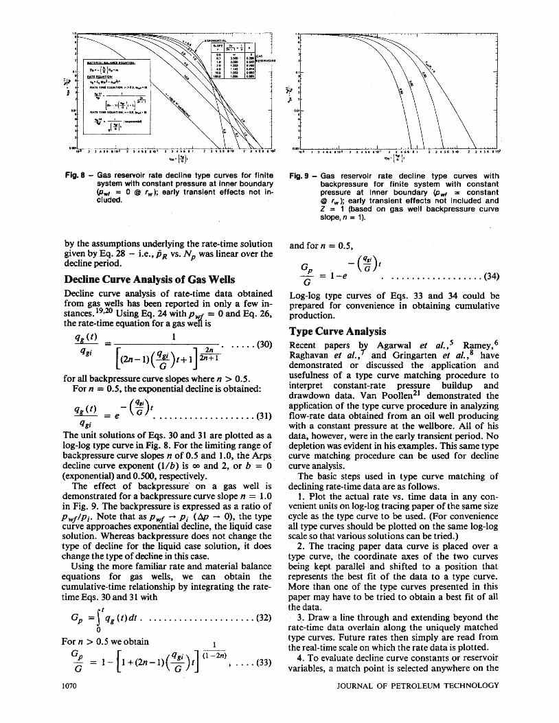
Fig. 8 - Gas reservoir rate decline type curves for finite system with constant pressure at inner boundary (Pwf = 0 @ ''II); early transient effects not in­cluded.

by the assumptions underlying the rate-time solution given by Eq. 28 - i.e., PR vs. Np was linear over the decline period.

Decline Curve Analysis of Gas Wells Decline curve analysis of rate-time data obtained from gas wells has been reported in only a few in­stances. 19,20 Using Eq. 24 with Pw1 = 0 and Eq. 26, the rate-time equation for a gas well is

qg (I) = 1 -----------. . .... (30)

qg; [(2n-1)(~ )/+ 1] 2n~t" for all backpressure curve slopes where n > 0.5.

For n = 0.5, the exponential decline is obtained:

q (I) - (q'i)t ~ = e G •••••••••••••••••••• (31)

qgi

The unit solutions of Eqs. 30 and 31 are plotted as a log-log type curve in Fig. 8. For the limiting range of backpressure curve slopes n of 0.5 and 1.0, the Arps decline curve exponent (lib) is 00 and 2, or b = O· (exponential) and 0.500, respectively.

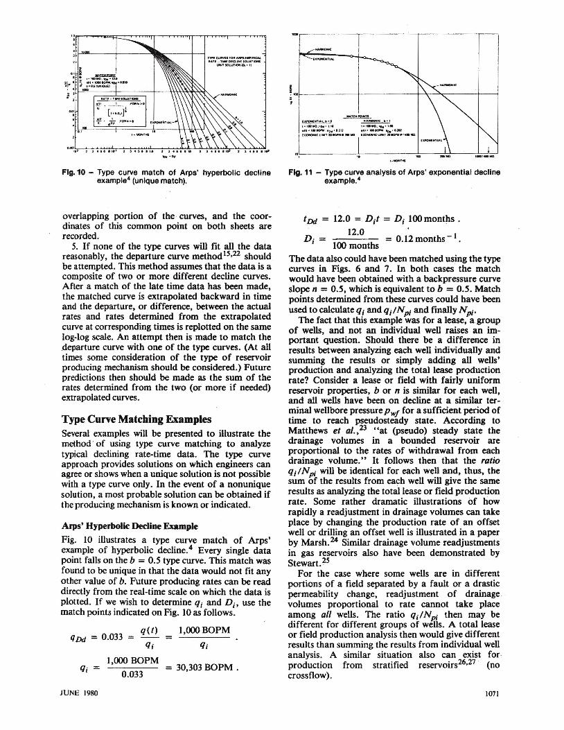
The effect of backpressure· on a gas well is demonstrated for a backpressure curve slope n = 1.0 in Fig. 9. The backpressure is expressed as a ratio of Pwj/Pi. Note that as Pwj - Pi (~ - 0), the type curve approaches exponential decline, the liquid case solution. Whereas backpressure does not change the type of decline for the liquid case solution, it does change the type of decline in this case.

Using the more familiar rate and material balance equations for gas wells, we can obtain the cumulative-time relationship by integrating the rate­time Eqs. 30 and 31 with

Gp = It qg (/)dt. . ..•................. (32) o

For n > 0.5 we obtain 1

G p [ ( q g;) ] (l - 2n) G = 1- 1 +(2n-l) G t , .... (33)

1070

':r~-""'I"'~~~~~~~..---,~~~--r~-'-"""'1

·

w: j 2

0 .01 · ·

Fig. 9 - Gas reservoir rate decline type curves with backpressure for finite system with constant pressure at Inner boundary (Pwf = constant @ ''II); early transient effects not included and Z = 1 (based on gas well backpressure curve slope, n = 1).

and for n = 0.5,

Gp - (~i)t - = l-e .................. (34) G

Log-log type curves of Eqs. 33 and 34 could be prepared for convenience in obtaining cumulative production.

Type Curve Analysis Recent papers ? Agarwal el al. ,S Ramey, 6

Raghavan el al., and Gringarten el al., 8 have demonstrated or discussed the application and usefulness of a type curve matching procedure to interpret constant-rate pressure buildup and drawdown data. Van Poollen21 demonstrated the application of the type curve procedure in analyzing flow-rate data obtained from an oil well producing with a constant pressure at the wellbore. All of his data, however, were in the early transient period. No depletion was evident in his examples. This same type curve matching procedure can be used for decline curve analysis.

The basic steps used in type curve matching of declining rate-time data are as follows.

1. Plot the actual rate vs. time data in any con­venient units on log-log tracing paper of the same size cycle as the type curve to be used. (For convenience all type curves should be plotted on the same log-log scale so that various solutions can be tried.)

2. The tracing paper data curve is placed over a type curve, the coordinate axes of the two curves being kept parallel and shifted to a position that represents the best fit of the data to a type curve. More than one of the type curves presented in this paper may have to be tried to obtain a best fit of all the data.

3. Draw a line through and extending beyond the rate-time data overlain along the uniquely matched type curves. Future rates then simply are read from the real-time scale on which the rate data is plotted.

4. To evaluate decline curve constants or reservoir variables, a match point is selected anywhere on the

JOURNAL OF PETROLEUM TECHNOLOGY

Twt! CU"VIES'Oft AN'S fWi",CAI.. "ATE - T .. IE OfClIN( EOUATIQIG

UNIT IOLU'TtOfilID, all

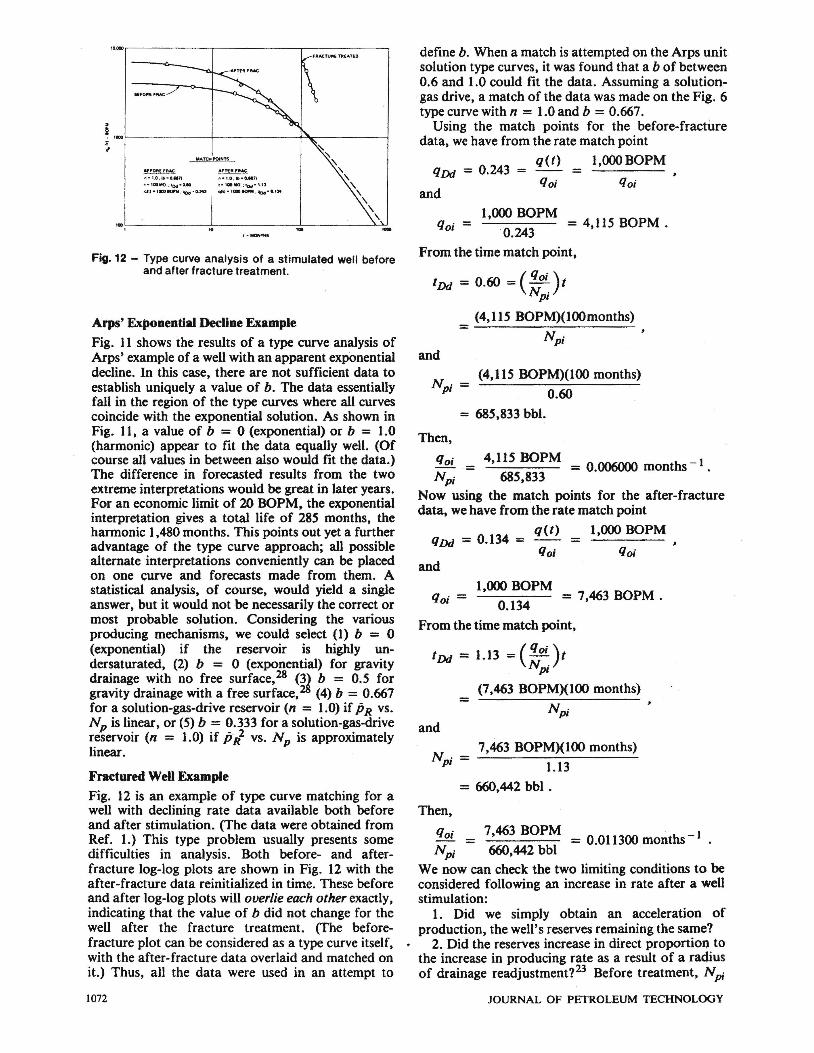
Fig. 10 - Type curve . match of Arps' hyperbolic decline example" (unique match).

overlapping portion of the curves, and the coor­dinates of this common point on both sheets are recorded.

5. If none of the type curves will fit all the data reasonably, the departure curve method 15,22 should be attempted. This method assumes that the data is a composite of two or more different decline curves. After a match of the late time data has been made, the matched curve is extrapolated backward in time and the departure, or difference, between the actual rates and rates determined from the extrapolated curve at corresponding times is replotted on the same log-log scale. An attempt then is made to match the departure curve with one of the type curves. (At all times some consideration of the type of reservoir producing mechanism should be considered.) Future predictions then should be made as the sum of the rates determined from the two (or more if needed) extrapolated curves.

Type Curve Matching Examples Several examples will be presented to illustrate the method· of using type curve matching to analyze typical declining rate-time data. The type curve approach provides solutions on which engineers can agree or shows when a unique solution is not possible with a type curve only. In the event of a nonunique solution, a most probable solution can be obtained if the producing mechanism is known or indicated.

Arps' Hyperbolic Decline Example

Fig. 10 illustrates a type curve match of Arps' example of hyperbolic decline.4 Every single data point falls on the b = 0.5 type curve. This match was found to be unique in that the data would not fit any other value of b. Future producing rates can be read directly from the real-time scale on which the data is plotted. If we wish to determine qj and D j , use the match points indicated on Fig. 10 as follows.

q(t) 1,000 BOPM qDd = 0.033 = - =

q; qj

q; =

JUNE 1980

1,000 BOPM = 30,303 BOPM .

0.033

I , *L---------~----------~~~----_+--~ , ..-.1C1t"".,1S

IlU'OtfIEN"Al. " "0 NAfWWUC • ., _ 1

,·'OOMO.; IDII '1.1' ,-,...0.:10.1" '._ "m-1ODIOf'II : 4D111"O.lll ""'" ltOtOf'II : lllo."O.lOl £COfrtOlillltC LIMIT 2Q IOHI. HI 110. ECONOMIC UMfT .110 ..... 1l1li MO

~ ,L __________ ~--------~ __ ~~--~~:~

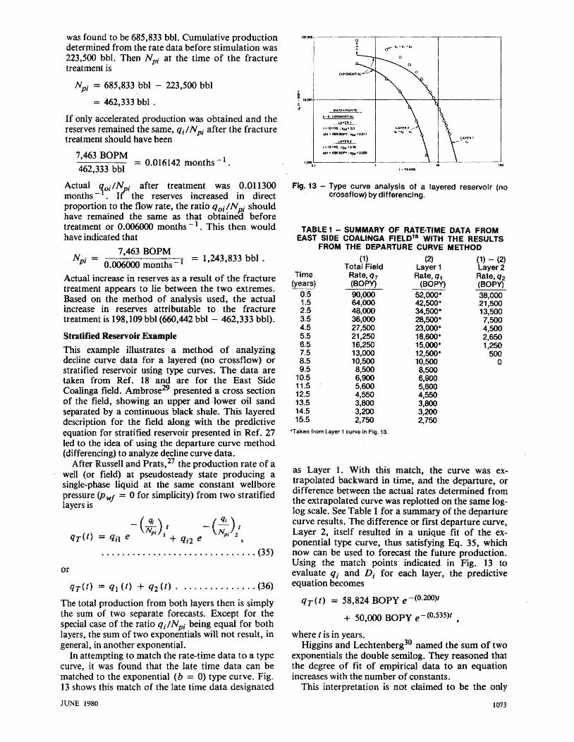
Fig. 11 - Type curve analYSis of Arps' exponential decline example."

tDd = 12.0 = Djt = D j 100 months .

12.0 -1 D; = = 0.12 months .

100 months The data also could have been matched using the type curves in Figs. 6 and 7. In both cases' the match would have been obtained with a backpressure curve slope n = 0.5, which is equivalent to b = 0.5. Match points determined from these curves could have been used to calculate q; and q j IN p; and finally N p;'

The fact that this example was for a lease, a group of wells, and not an individual well raises an im­portant question. Should there be a difference in results between analyzing each well individually and summing the results or simply adding all wells' production and analyzing the total lease production rate? Consider a lease or field with fairly uniform reservoir properties, b or n is similar for each well, and all wells have been on decline at a similar ter­minal wellbore pressure Pwf for a sufficient pe~od of time to reach ~udosteady state. According to Matthews et al.,23 "at (pseudo) steady state the drainage volumes in a bounded reservoir are proportional to the rates of withdrawal from each drainage volume." It follows then that the ratio q;INp ; will be identical for each well and, thus, the sum of the results from each well will give the same results as analyzing the total lease or field production rate. Some rather dramatic illustrations of how rapidly a readjustment in drainage volumes can take place by changing the production rate of an offset well or drilling an offset well is illustrated in a paper by Marsh. 24 Similar drainage volume readjustments in gas reservoirs also have been demonstrated by Stewart. 25

For the case where some wells are in different portions of a field separated by a fault or a drastic permeability change, readjustment of drainage volumes proportional to rate cannot take place among all wells. The ratio qjlNl!i then may be different for different groups of wells. A total lease or field production analysis then would give different results than summing the results from individual well analysis. A similar situation also can exist for ­production from stratified reservoirs26,27 (no crossflow).

1071

'O_r--~----r--------r---------'

~ ~ ,,- 1.0." -a .• 7, ,, -I.o , 8I-o.a71 .-looMO. ; ,OoiI.'"O . ., . -II1DMO.;lo.-I .1l

qf1)-loaDl()IIIM ; "Od'"O.XJ ~'I"I000IOP'lllll ; ~·O.I"

,~ L, ____ ~~_---~~_--~~

Fig. 12 - Type curve analysis of a stimulated well before and after fracture treatment.

Arps' Exponential Decline Example Fig. 11 shows the results of a type curve analysis of Arps' example of a well with an apparent exponential decline. In this case, there are not sufficient data to establish uniquely a value of b. The data essentially fall in the region of the type curves where all curves coincide with the exponential solution. As shown in Fig. 11, a value of b = 0 (exponential) or b = 1.0 (harmonic) appear to fit the data equally well. (Of course all values in between also would fit the data.) The difference in forecasted results from the two extreme interpretations would be great in later years. For an economic limit of 20 BOPM, the exponential interpretation gives a total life of 285 months, the harmonic 1,480 months. This points out yet a further advantage of the type curve approach; all possible alternate interpretations conveniently can be placed on one curve and forecasts made from them. A statistical analysis, of course, would yield a single answer, but it would not be necessarily the correct or most probable solution. Considering the various producing mechanisms, we could select (1) b = 0 (exponential) if the reservoir is highly un­dersaturated, (2) b = 0 (exponential) for gravity drainage with no free surface,28 (n b = 0.5 for gravity drainage with a free surface, (4) b = 0.667 for a solution-gas-drive reservoir (n = 1.0) if jJ R vs. Np is linear, or (5) b = 0.333 for a solution-gas-drive reservoir (n = 1.0) if jJIl vs. Np is approximately linear.

Fractured Well Example Fig. 12 is an example of type curve matching for a well with declining rate data available both before and after stimulation. (The data were obtained from Ref. 1.) This type problem usually presents some difficulties in analysis. Both before- and after­fracture log-log plots are shown in Fig. 12 with the after-fracture data reinitialized in time. These before and after log-log plots will overlie each other exactly, indicating that the value of b did not change for the well after the fracture treatment. (The before­fracture plot can be considered as a type curve itself, . with the after-fracture data overlaid and matched on it.) Thus, all the data were used in an attempt to

J072

define b. When a match is attempted on the Arps unit solution type curves, it was found that a b of between 0.6 and 1.0 could fit the data. Assuming a solution­gas drive, a match of the data was made on the Fig. 6 type curve with n = 1.0 and b = 0.667.

Using the match points for the before-fracture data, we have from the rate match point

qDd = 0.243 = q(t) = I,OOOBOPM qo; qo;

and

1,000 BOPM qo; =

0.243 = 4,115 BOPM .

From the time match point,

tDd = 0.60 = (qo;.)t Npl

and

Then,

= (4,115 BOPM)(I00months)

(4,115 BOPM)(100 months)

0.60

= 685,833 bbl.

qo; 4,115 BOPM 0006000 h -I = =. mont s . N p; 685,833

Now using the match points for the after-fracture data, we have from the rate match point

qDd = 0.134 = q(t) = 1,000 BOPM qo; qoi

and

1,000 BOPM = 7 463 BOPM . qoi = 0.134 '

From the time match point,

tDd = 1.13 = (::i.)t pi

(7,463 BOPM)(I00 months) = Np;

and

7,463 BOPM)(I00 months) N p; = -----------

1.13

= 660,442 bbl .

Then,

qo; = 7,463 BOPM = 0.011300 months-I Npi 660,442 bbl

We now can check the two limiting conditions to be considered following an increase in rate after a well stimulation:

1. Did we simply obtain an acceleration of production, the well's reserves remaining the same?

2. Did the reserves increase in direct proportion to the increase in producing rate as a result of a raclius of drainage readjustment?23 Before treatment, N p;

JOURNAL OF PETROLEUM TECHNOLOGY

was found to be 685,833 bbl. Cumulative production determined from the rate data before stimulation was 223,500 bbl. Then Npi at the time of the fracture treatment is

Npi = 685,833 bbl - 223,500 bbl

= 462,333 bbl .

If only accelerated production was obtained and the reserves remained the same, qilNpi after the fracture treatment should have been

7,463 BOPM _ -I 462,333 bbl - 0.016142 months

Actual ~oilN i after treatment was 0.011300 months - . If the reserves increased in direct proportion to the flow rate, the ratio q oi IN pJ should have remained the same as that obtained before tteatment or 0.006000 months -I. This then would have indicated that

N . = 7,463 BOPM pi 0.006000 months- 1 = 1,243,833 bbl.

Actual increaSe in reserves as a result of the fracture tteatment appears to lie between the two extremes. Based on the method of analysis used, the actual increase in reserves attributable to the fracture treatment is 198,109 bbl (660,442 bbl - 462,333 bbl).

Stratified Reservoir ExaiDpie

This example illustrates a method of analyzing decline curve data for a layered (no crossflow) or stratified reservoir using type curves. The data are taken from Ref. 18 and are for the East Side Coalinga field. Ambrose29 presented a cross section of the field, showing an upper and lower oil sand separated by a continuous black shale. This layered description for the field along with the predictive equation for stratified reservoir presented in Ref. 27 led to the idea of using the departure curve method (differencing) to analyze decline curve data.

After Russell and Prats,27 the production rate of a well (or field) at pseudosteady state producing a single-phase liquid at the same constant wellbore pressure (Pwj = 0 for simplicity) from two stratified layers is

-(~) ( -(~) t Np; I N · 2

qr(t) = qil e + qi2 e PI,

.......... . ....... . ........... (35)

or

qr(t) = ql (t) + q2 (I) .. . ............ (36)

The total production from both layers then is simply the sum of two separate forecasts. Except for the special case of the ratio qilNpi being equal for both layers, the sum of two exponentials will not result, in general, in another exponential.

In attempting to match the rate-time data to a type curve, it was found that the late time data can be matched to the exponential (b = 0) type curve. Fig. 13 shows this match of the late time data designated

JUNE 1980

l00.00Dr-- ----::-----,-- - --- ,- - - - - -- -,

!

, •. 00Df-------+---~----'*-----___I

b .. U. EXroHf.NTIAl

1 "10l''''.; ~·2.0

'·,O'fftS. ; to.a .... Ja

1liII' -tmolOP'Y ; 4CN'"6.DIO

I ,OODDL.l _ _ ___ -L-___ _ .I.....-4_-'-_ __ --:-!.

Fig. 13 - Type curve analysis of a layered reservoir (no crossflow) by differencing.

TABLE1 - SUMMARY OF RATE·TIME DATA FROM EAST SIDE COALINGA FIELD18 WITH THE RESULTS

FROM THE DEPARTURE CURVE METHOD

(1) (2) (1) - (2) Total Field Layer 1 Layer 2

Rate, qr Rate, q1 Rate, q2 (BOPy) (BOPy) (BOPy)

Time (years)

0.5 1.5 2.5 3.5 4.5 5.5 6.5 7.5 8.5 9.5

10.5 11.5 12.5 13.5 14.5 15.5

90,000 64,000 48,000 36,000 27,500 21,250 16,250 13,000 10,500 8,500 6,900 5,600 4,550 3,800 3,200 2,750

-Taken from layer 1 curve in Fig. 13.

52,000· 42,500· 34,500" 28,500· 23,000" 18,600" 15,000· 12,500· 10,500 8,500 6,900 5,600 4,550 3,800 3,200 2,750

38,000 21,500 13,500 7,500 4,500 2,650 1,250

500 o

as Layer 1. With this match, the curve was ex­trapolated backward in time, and the departure, or difference between the actual rates determined from the extrapolated curve was replotted on the same log­log scale. See Table 1 for a summary of the departure curve results. The difference or first departure curve, Layer 2, itself resulted in a unique fit of the ex­ponential type curve, thus satisfying Eq. 35, which now can be used to forecast the future production. Using the match points indicated in Fig. 13 to evaluate qi and Di for each layer, the predictive equation becomes

qr(t) = 58,824 BOPY e-(O.200)t

+ 50,000 BOPY e - (0.535)( ,

where t is in years. Higgins and Lechtenberg30 named the sum of two

exponentials the double semilog. They reasoned that the degree of fit of empirical data to an equation increases with the number of constants.

This interpretation is not claimed to be the only

1073

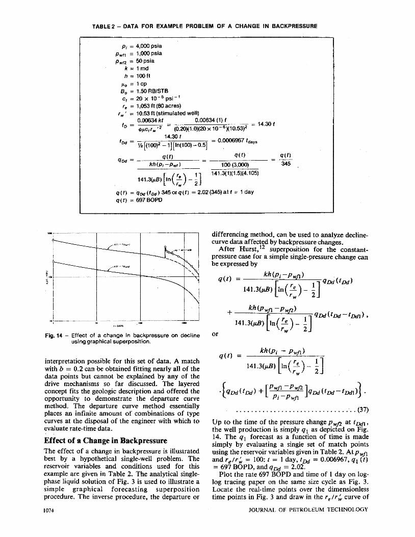
TABLE 2 - DATA FOR EXAMPLE PROBLEM OF A CHANGE IN BACKPRESSURE

Pi = 4,000 psia Pwf1 = 1,000 psi a Pwf2 = 50 psia

k = 1 md h=100ft

P.o = 1 cp 8 0 = 1.50 RB/STB c t = 20 X 10-6 psi- 1

fe = 1,053 ft (80 acres) f w' = 10.53 ft (stimulated well)

0.()()634 kt 0.00634 (1) t 10 - - 2 = 14.30 t

- q,p.Ct f w,2 -(0.20)(1.0)(20x10 6)(10.53)

14.30 t IOd = = 0.0006967 tdays

Y2 [(100)2 -1][ln(1oo) - 0.5]

q(t) q Od = ---:--:--....!...:.-"------

kh(p;-Pwf)

q(t)

100 (3,000)

q(t)

345

[ ( ) 1] 141.3(1)(1.5)(4.105)

141.3(p.8) In ;: - 2 q (t) =qOd (tOd) 345 or q( t) = 2.02 (345) at I = 1 day q (t) = 697 BOPO

~ I.i--------+------='t=-_=c----+--"'c1

,.l, _____ ~L_ _____ , .. L--_-_-~---"

Fig. 14 - Effect of a change in backpressure on decline using graphical superposition.

interpretation possible for this set of data. A match with b = 0.2 can be obtained fitting nearly all of the data points but cannot be explained by any of the drive mechanisms so far discussed. The layered concept fits the geologic description and offered the opportunity to demonstrate the departure curve method. The departure curve method essentially places an infinite amount of combinations of type curves at the disposal of the engineer with which to evaluate rate-time data.

Effect of a Change in Backpressure The effect of a change in backpressure is illustrated best by a hypothetical single-well problem. The reservoir variables and conditions used for this example are given in Table 2. The analytical single­phase liquid solution of Fig. 3 is used to illustrate a simple graphical forecasting superposition procedure. The inverse procedure, the departure or

1074

differencing method, can be used to analyze decline­curve data affected by backpressure changes.

After Hurst,12 superposition for the constant­pressure case for a simple single-pressure change can be expressed by

q(t) = [ ] qDd(IDd) 141.3(p..8) In( re ) _ !

rw 2

kh (Pwfl - Pwp.)

or

q(t) =

................................ (37)

Up to the time of the pressure change P wj2 at IDdI' the well production is simply q 1 as depicted on Fig. 14. The ql forecast as a function of time is made simply by evaluating a single set of match points using the reservoir variables given in Table 2. At PwfJ. and re/r ~ = 100: I = 1 day, IDd = 0.006967, ql (I) = 697 BOPO, and qDd = 2.02.

Plot the rate 697 BOPO and time of 1 day on log­log tracing paper on the same size cycle as Fig. 3. Locate the real-time points over the dimensionless time points in Fig. 3 and draw in the re/r ~ curve of

JOURNAL OF PETROLEUM TECHNOLOGY

TABLE 3 - COMPARISONS OF kh DETERMINED FROM BUILDUP AND DECLINE CURVE ANALYSIS, FIELD A (SANDSTONE RESERVOIR);

160·ACRE SPACING,'. = 1,490 ft,'w = 0.25 ft Pressure Buildup Results

Well h If> Swc Skin f ' w kh No. J!!L (%) (%) s J!!L (md-ft) - --

1 34 9.4 32.9 -0.23 0.3 120.5 2 126 10.5 18.3 -2.65 3.5 56.7 3 32 9.9 20.4 -3.71 10.3 63.0 4 63 9.5 18.6 - 3.41 7.6 28.5 5 67 10.2 15.1 -4.29 18.3 44.4 6 28 10.3 12.6 -2.07 2.0 57.9 7 17 10.0 17.5 -3.41 7.6 16.8 8 47 9.1 24.2 -3.74 10.6 16.6 9 87 10.2 18.0 -4.19 16.5 104.7

10 40 10.4 21.7 -5.80 82.9 363.2 11 29 11.5 19.2 -1.00 2.0 59.9 12 19 11.1 17.0 -3.97 13.3 8.9 13 121 10.1 18.8 -3.85 11.8 47.5 16 74 9.4 20.4 -4.10 15.0 224.8 15 49 10.9 28.6 -3.59 9.1 101.9 16 35 10.0 25.6 -4.57 24.2 14.3 17 62 8.8 22.4 -3.12 5.7 27.2 18 75 9.4 18.1 -1.50 1.2 65.1 19 38 8.9 19.2 - 2.11 2.1 40.5 20 60 9.6 24.6 . -5.48 60.1 88.1 21 56 11.1 16.5 -2.19 2.2 39.1 22 40 8.9 22.5 -3.79 11.1 116.0

·'w' used from buildup analysis with'e of 1,490 ft.

100 on the tracing paper. Read flow rates as a function of time directly from the real-time scale.

When a change in pressure is made to P w/l at t 1 , t = 0 for the accompanying change in rate q2 (really a tlq for superposition), this rate change retraces the q Dd vs. t Dd curve and is simply a constant fraction of ql :

q _ q [Pw/l-PW/2] , 2 - 1 Pi-Pw/l

or at t - 1 day after the rate change,

[ 1,000 psi - 50 psi ]

q2 = 697 BOPD 4,000 psi - 1,000 psi = 221 BOPD.

The total rate qT after the pressure change is qT = ql + q2 as depicted in Fig. 14. Flow rates for this example were read directly from the curves in Fig. 14 and summed at times past the pressure change Pwfl.

The practical application of this example in decline curve analysis is that the departure or difference method can be used on rate-time data affected by a change in backpressure. The departure curve represented by q2 in Fig. 14 should overlie exactly the curve represented by q l' If it does in an actual field example, the future forecast is made correctly by extending both curves and summing them at times beyond the pressure change_

Calculation of kh From Decline Curve Data Pressure buildup and decline curve data were available from a high-pressure, highly un­dersaturated, low-permeability sandstone reservoir. Initial reservoir pressure was estimated to be 5,790

JUNE 1980

Decline Curve Analysis Results

fe1fw ,

qDd Pi-Pwf kh k Matched (10,000 BOPM) (1'0 8 0 ) (md-ft) (md)

0.52 6658 108 3.18 0.68 7979 48 0.38 0.43 8048 60 1.88

40 0.58 8273 31 0.49 20 0.57 6296 32 0.48

0.60 7624 62 2.21 10 1.30 7781 8.3 0.49 10 1.14 7375 10 0.21

0.435 5642 76 0.87 0.36 1211 255 ·6.38 0.56 7669· 66 2.28

50 3.30 5045 9.5 0.50 50 0.54 7259 40.5 0.33

0.32 5737 104 1.41 0.43 4312 115 2.35

20 0.96 5110 24 0.69 0.82 8198 35 0.56 0.52 6344 93 1.24

20 0.54 6728 32 0.84 0.345 5690 64 1.07

20 0.72 5428 30 0.54 100 0.46 8114 51 1.28

'·."<--<;:---------------O' .. ::c-NS:-'ONc-:":-SSF:-::LOW:-A:-.,'~FU:-N"'=>ONS=---:j

6 l"'fINm,.~:~~I:::~llJ~~~UND ... RY.

0.' . ~~ . qo[,nl;;l-~]-~

t.1.3l't~ft(;;)_j] »

CONSTANT-rftESSUftf AllNNER BOUNOAR'f'

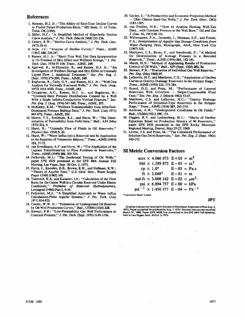
Fig. 15 - Type curve matching example for calculating kh using decline curve data, Well 13, Field A.

"'!~--;;-'O-=VS"'-IOL F=O'C:-:AVC::"=To<ACCC"C:-, -------

~ FRACTURED W~LL IANAl.YTIC"L SOlN.! . ,

} : iooo

Fig. 16 - Type curve matching example for calculating kh from pressure buildup data, Well 13, Field A (type curve from Ref. 8).

1075

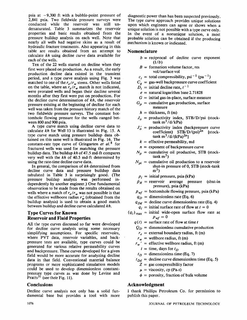
psi a at - 9,300 ft with a bubble-point pressure of 2,841 psia. Two fieldwide pressure surveys were conducted while the reservoir was still Un­dersaturated. Table 3 summarizes the reservoir properties and basic results obtained from the pressure buildup analysis on each well. Note that nearly all wells had negative skins as a result of hydraulic fracture treatments. Also appearing in this table are results obtained from an attempt to calculate kh using decline curve data available for each of the wells.

Ten of the 22 wells started on decline when they first were placed on production. As a result, the early production decline data existed in the transient period, and a type curve analysis using Fig. 3 was matched to one ofthe 'elr w stems. Other wells listed on the table, where an 'elr w match is not indicated, were prorated wells and began their decline several months after they first were put on production. For the decline curve determination of kh, the reservoir pressure existing at the beginning of decline for each well was taken from the pressure history match of the two fieldwide pressure surveys. The constant bot­tomhole flowing pressure for the wells ranged bet­ween 800 and 900 psia.

A type curve match using decline curve data to calculate kh for Well 13 is illustrated in Fig. 15. A type curve match using pressure buildup data ob­tained on this same well is illustrated in Fig. 16. The constant-rate type curve of Gringarten et 01.8 for fractured wells was used for matching the pressure buildup data. The buildup kh of 47.5 md-ft compares very well with the kh of 40.5 md-ft determined by using the rate-time decline curve data.

In general, the comparison of kh determined from decline curve data and pressure buildup data tabulated in Table 3 is surprisingly good. (The pressure buildup analysis was performed in­dependently by another engineer.) One fundamental observation to be made from the results obtained on wells where a match of rei r w was not possible is that the effective wellboore radius r; (obtained from the buildup analysis) is used to obtain a good match between buildup and decline curve calculated kh.

Type Curves for Known Reservoir and Fluid Properties All the type curves discussed so far were developed for decline curve analysis using some necessary simplifying assumptions. For specific reservoirs, where PVT data, reservoir variables, and back­pressure tests are available, type curves could be generated for various relative permeability curves and backpressure. These curves developed for a given field would be more accurate for analyzing decline data in that field. Conventional material balance programs or more sophisticated simulation models could be used to develop dimensionless constant­pressure type curves as was done by Levine and Pratts31 (see their Fig. 11).

Conclusions Decline curve analysis not only has a solid fun­damental base but provides a tool with more

1076

diagnostic power than has been suspected previously. The type curve approach provides unique solutions upon which engineers can agree or shows when a unique solution is not possible with a type curve only. In the event of a nonunique solution, a most probable solution can be obtained if the producing mechanism is known or indicated.

Nomenclature b = reciprocal of decline curve exponent

(lib) B = formation volume factor, res

vol/surface vol C t = total compressibility, psi - 1 (pa - 1 )

C g = gas-well back pressure curve coefficient D i = initial decline rate, t - 1

e = natural logarithm base 2.71828 G = initia~ gas-in-place, surface measure

G p = cumulative gas production, surface measure

h = thickness, ft (m) J 0 = productivity index, STB/D/psi (stock­

tank m 3 I d/kPa) J ~ = productivity index (backpressure curve

coefficient) STB/D/(psi)2n [stock­tank m3/d/(kPa)2n]

k = effective permeability, md n = exponent of backpressure curve

Np = cumulative oil productive, STB (stock­tank m 3 )

Npi = cumulative oil production to a reservoir shut-in pressure of 0, STB (stock-tank m 3)

Pi = initial pressure, psia (kPa) P R = reservoir average pressure (shut-in

pressure), psia (kPa) Pwf = bottomhole flowing pressure, psia (kPa) qD == dimensionless rate (Eq. 6)

qDd = decline curve dimensionless rate (Eq. 4) q i = initial surface rate of flow at t = 0

(q i) max = initial wide-open surface flow rate at Pwf = 0

q (t) = surface rate of flow at time t QD = dimensionless cumulative production 'e = external boundary radius, ft (m) 'w = wellbore radius, ft (m)

, w' = effective well bore radius, ft (m) I = time, days for tD

I D = dimensionless time (Eq. 7) t Dd = decline curve dimensionless time (Eq. 5)

Z = gas compressibility factor I" = viscosity, cp (Pa.s) 4> = porosity, fraction of bulk volume

Acknowledgment I thank Phillips Petroleum Co. for permission to publish this paper.

JOURNAL OF PETROLEUM TECHNOLOGY

References 1. Ramsay, H.J. Jr.: "The Ability of Rate-Time Decline Curves

to Pr~ict Future Production Rates," MS thesis, U. of Tulsa, Tulsa, OK (1968).

2. Slider, H.C.: "A Simplified Method of Hyperbolic Decline Curve Analysis." J. Pet. Tech. (March 1968) 235-236.

3. Gentry, R.W.: "Decline-Curve Analysis," J. Pet. Tech. (Jan. 1972) 38-41. .

4. Arps, J.J.: "Analysis of Decline Curves," Trans., AlME (1945) 160, 228-247.

5. Ramey, H.J. !r.: "Short-Time Well Test Data Interpretation in the Presence of Skin Effect and Wellbore Storage," J. Pet. Tech. (Jan. 1970) 97-104; Trans., AlME, 149.

6. Agarwal, R., Al-Hussainy, R., and Ramey, H.J. Jr.: "An Investigation of Wellbore Storage and Skin Effect in Unsteady Liquid Flow: I. Analytical Treatment," Soc. Pet. Eng. J. (Sept. 1970) 279-290; Trans., AlME, 149.

7. Raghavan, R., Cady, G.V., and Ramey, H.J. Jr.: "Well-Test Analysis for Vertically Fractured Wells," J. Pet. Tech. (Aug. 1972) 1014-1020; Trans., AlME,lS3.

8. Gringarten, A.C., Ramey, H.J. Jr., and Raghavan, R.: "Unsteady-State Pressure Distributions Created by a Well With a Single Infinite-Conductivity Vertical Fracture," Soc. Pet. Eng. J. (Aug. 1974) 347-360; Trans., AIME,'lS7.

9. McKinley, R.M.: "Wellbore Transmissibility from Afterflow­Dominated Pressure Buildup Data," J. Pet. Tech. (July 1971) 863-872; Trans., AlME, 251.

10. Moore, T.V., Schilthuis, R.J., and Hurst, W.: "The Deter­mination of Permeability from Field Data," Bull., API (May 1933) 111, 4.

11. Hurst, R.: "Unsteady Flow of Fluids in Oil Reservoirs:' Physics(Jan. 1934) 5, 20.

12. Hurst, W.: "Water Influx into a Reservoir and Its Application to the Equation of Volumetric Balance," Trans., AIME (1943) 151,57-72.

13. van Everdingen, A.F. and Hurst, W.: "The Application of the Laplace Transformation to Flow Problems in Reservoirs," Trans., AlME (1949) 186,305-314.

14. Fetkovich, M.J.: "The Isochronal Testing of Oil Wells," paper SPE 4529 presented at the SPE 48th Annual Fall Meeting, Las Vegas, Sept. 30-0ct. 3, 1973.

15. Ferris, J.,Knowles, D.B., Brown, R.H., and Stallman, R.W.: "Theory of Aquifer Tests," U.S. Geo/. Surv., Water Supply Paper 1536E(1962) 109. -

16. Tsarevich, K.A. and Kuranov, I.F.: "Calculation of the Flow Rates for the Center Well in a Circular Reservoir Under Elastic Conditions," Problems of Reservoir Hydrodynamics, Leningrad (1966) Part I, 9-34.

17. Fetkovich, M.J.: "A Simplified Approach to Water Influx Calculations-Finite Aquifer Systems," J. Pet. Tech. (July 1971) 814-823.

18. Cuttler, W. W. Jr.: "Estimation of Underground Oil Reserves by Oil-Well Production Curves," Bull., USBM (1924) 228.

19. Stewart, P.R.: "Low-Permeability Gas Well Performance at Constant Pressure," J. Pet. Tech. (Sept. 1970) 1149-1156.

JUNE 1980

20. Gurley, J.: "A Productivity and Economic Projection Method - Ohio Clinton Sand Gas Wells," J. Pet. Tech. (Nov. 1963) 1183-1185.

21. van Poollen, H.K.: "How to Analyze Flowing Well-Test Data ... with Constant. Pressure at the Well Bore," Oil and Gas J. (Jan. 16, 1967) 98-101.

22. Witherspoon, P.A., Javandel, I., Neuman, S.P., and Freeze, P .A.: Interpretation of Aquifer Gas Storage Conditions from Water Pumping Tests, Monograph, AGA, New York City (1967) 110.

23. Matthews, C.S., Brons, F., and Hazebroek, P.: "A Method for Determination of Average Pressure in a Bounded Reservoir," Trans., AIME (1954) 201, 182-191.

24. Marsh, H.N.: "Method of Appraising Results of Production Control of Oil Wells," Bull., API (Sept. 1928) lIl, 86.

25. Stewart, P.R.: "Evaluation oflndividual Gas Well Reserves," Pet. Eng. (May 1966) 8S.

26. Lefkovits, H.C. and Matthews, C.S.: "Application of Decline Curves to Gravity-Drainage Reservoirs in the Stripper Stage," Trans., AlME (l9S8) 113, 275-284.

27. Russel, D.G. and Prats, M.: "Performance of Layered Reservoirs With Cross flow - Single-Compressible Fluid Case," Soc, Pet. Eng. J. (March 1962) 53-67.

28. Matthews, C.S. and Lefkovits, H.C.: "Gravity Drainage Performance of Depletion-Type Reservoirs in the Stripper Stage," Trans., AIME (1956) 207, 265-274.

29. Ambrose, A.W.: "Underground Conditions in Oil Fields," Bull., USBM (1921) 195,151.

30. Higgins, R.V. and Lechtenberg, H.J.: "Merits of Decline Equations Based on Production History of 90 Reservoirs," paper SPE 2450 presented at the SPE Rocky Mountain Regional Meeting, Denver, May 25-27, 1969.

31. Levine, J.S. and Prats, M.: "The Calculated Performance of Solution-Gas Drive Reservoirs," Soc. Pet. Eng. J. (Sept. 1961) 142-152.

SI Metric Conversion Factors

acre x 4.046 873 E+03 m2

bbl x 1.589873 E-Ol = m3

cp x 1.0* E-03 Pa.s ft x 3.048* E-Ol = m

md-ft x 3.008 142 E+02 ,an2. psi x 6.894 757 E+OO kPa

psi -1 x 1.450377 E-04 Pa- 1

·Conversion factor is exact.

JPT

Original manuscript received In Society of Petroleum Engineers office Aug. 3, 1973. Paper accepted for publication Aug. 7, 1974. Revised manuscript received March 31, 1980. Paper (SPE 4629) first presented at the SPE 48th Fall Meeting, held In Las Vegas, Sept. 3().()ct. 3, 1973.

1077