Embed Size (px)
Citation preview
EOS Data ProductsHandbook
Volume 2
ACRIMSAT • Aqua • Jason-1 • Landsat 7• Meteor 3M/SAGE III •
QuikScat • QuikTOMS • VCL
EO
S Data P
roducts Handbook
• Volume 2
National Aeronautics andSpace Administration NP-2000-5-055-GSFC
ACRIMSAT• ACRIM III
Aqua• AIRS• AMSR-E• AMSU-A• CERES• HSB• MODIS
Jason-1• DORIS• JMR• Poseidon-2
Landsat 7• ETM+
Meteor 3M• SAGE III
QuikScat• SeaWinds
QuikTOMS• TOMS
VCL• MBLA
EOShttp://eos.nasa.gov/
EOSDIShttp://spsosun.gsfc.nasa.gov/New_EOSDIS.html

EOS Data ProductsHandbookVolume 2
ACRIMSAT• ACRIM III
Aqua• AIRS
• AMSR-E• AMSU-A
• CERES• HSB
• MODIS
Jason-1• DORIS
• JMR• Poseidon-2
Landsat 7• ETM+
Meteor 3M• SAGE III
QuikScat• SeaWinds
QuikTOMS• TOMS
VCL• MBLA

EditorsClaire L. Parkinson
NASA Goddard Space Flight Center
Reynold GreenstoneRaytheon ITSS
Design and ProductionSterling Spangler
For Additional Copies:EOS Project Science Office
Code 900NASA/Goddard Space Flight Center
Greenbelt, MD 20771http://eos.nasa.gov
Phone: (301) 441-4259Internet: [email protected]
NASA Goddard Space Flight CenterGreenbelt, Maryland
Printed October 2000
EOS Data ProductsHandbook
Volume 2
AcknowledgmentsSpecial thanks are extended toMichael King for guidancethroughout and to the many addi-tional individuals who also pro-vided information necessary for thecompletion of this second volumeof the EOS Data Products Hand-book. These include most promi-nently Stephen W. Wharton andMonica Faeth Myers, whose tre-mendous efforts brought aboutVolume 1, and the members of thescience teams for each of the in-struments covered in this volume.
Support for production of thisdocument, provided by WilliamBandeen, Jim Closs, Steve Gra-ham, and Hannelore Parrish, is alsogratefully acknowledged.
Raytheon ITSS

Abstract
The EOS Data Products Handbook provides brief descriptions of the data prod-ucts that will be produced from a range of missions of the Earth ObservingSystem (EOS) and associated projects. Volume 1, originally published in 1997,covers the Tropical Rainfall Measuring Mission (TRMM), the Terra mission(formerly named EOS AM-1), and the Data Assimilation System, while thisvolume, Volume 2, covers the Active Cavity Radiometer Irradiance MonitorSatellite (ACRIMSAT), Aqua, Jason-1, Landsat 7, Meteor 3M/StratosphericAerosol and Gas Experiment III (SAGE III), the Quick Scatterometer (Quik-Scat), the Quick Total Ozone Mapping Spectrometer (QuikTOMS), and theVegetation Canopy Lidar (VCL) missions. Volume 2 follows closely the formatof Volume 1, providing a list of products and an introduction and overviewdescriptions of the instruments and data processing, all introductory to the coreof the book, which presents the individual data product descriptions, organizedinto 11 topical chapters. The product descriptions are followed by five appendi-ces, which provide contact information for the EOS data centers that will bearchiving and distributing the data sets, contact information for the science pointsof contact for the data products, references, acronyms and abbreviations, and adata products index.
I

Abstract I
Foreword IV
List of Data Products (Organized by Mission Name) 1
Introduction 11
Instrument Descriptions and Data Processing Overviews 15
Radiance/Reflectance and Irradiance Products 47
Precipitation and Atmospheric Humidity 71
Cloud and Aerosol Properties and Radiative Energy Fluxes 87
Atmospheric Chemistry 123
Atmospheric Temperatures 131
Winds 139
Sea Surface Height and Ocean Wave Dynamics 147
Surface Temperatures of Land and Oceans, Fire Occurrence, and Volcanic Effects 151
Vegetation Dynamics, Land Cover, and Land Cover Change 165
Phytoplankton and Dissolved Organic Matter 187
Snow and Ice Cover 203
Appendix A: EOS Distributed Active Archive Centers (DAACs) Contact Information 217
Appendix B: Points of Contact 218
Appendix C: References 225
Appendix D: Acronyms and Abbreviations 246
Appendix E: Data Products Index (Organized by Instrument Name) 252
Table of Contents
○ ○ ○ ○ ○ ○ ○ ○ ○ ○ ○
○ ○ ○ ○ ○ ○ ○ ○ ○ ○ ○ ○ ○ ○ ○ ○ ○ ○ ○ ○ ○ ○ ○ ○ ○ ○ ○ ○ ○ ○ ○
○ ○ ○ ○ ○ ○ ○
○ ○ ○ ○ ○ ○ ○ ○ ○ ○ ○ ○ ○
○ ○ ○ ○ ○ ○ ○ ○ ○ ○ ○ ○ ○ ○ ○ ○
○ ○ ○ ○ ○ ○
○ ○ ○ ○ ○ ○ ○ ○ ○ ○ ○ ○ ○ ○ ○ ○ ○ ○ ○ ○ ○ ○ ○
○ ○ ○ ○ ○ ○ ○ ○ ○ ○ ○ ○ ○ ○ ○ ○ ○ ○ ○ ○ ○ ○
○ ○ ○ ○ ○ ○ ○ ○ ○ ○ ○ ○ ○ ○ ○ ○ ○ ○ ○ ○ ○ ○ ○ ○ ○ ○ ○ ○ ○ ○ ○ ○
○ ○ ○ ○ ○ ○ ○ ○ ○ ○ ○ ○
○ ○ ○ ○ ○ ○ ○ ○ ○ ○ ○ ○ ○ ○ ○
○ ○ ○ ○ ○ ○
○ ○ ○ ○ ○ ○ ○ ○ ○ ○ ○ ○ ○
○ ○ ○ ○ ○ ○ ○ ○ ○ ○ ○ ○ ○ ○ ○ ○ ○ ○ ○ ○ ○ ○ ○ ○ ○
○ ○ ○ ○ ○ ○ ○ ○ ○ ○ ○ ○ ○ ○ ○ ○ ○ ○ ○ ○ ○ ○ ○
○ ○ ○ ○ ○ ○ ○ ○ ○ ○ ○ ○ ○ ○ ○ ○ ○ ○ ○
○ ○ ○ ○ ○ ○ ○ ○ ○ ○ ○ ○ ○ ○
○ ○
○ ○ ○ ○ ○ ○ ○ ○ ○ ○ ○ ○ ○ ○ ○ ○ ○ ○ ○ ○
III
○ ○ ○ ○ ○ ○ ○ ○ ○ ○ ○ ○ ○ ○ ○ ○ ○ ○ ○ ○ ○ ○ ○ ○ ○ ○ ○ ○ ○ ○ ○ ○ ○
○ ○ ○ ○ ○ ○ ○ ○ ○ ○ ○ ○ ○ ○ ○ ○ ○ ○ ○ ○ ○ ○ ○ ○ ○ ○ ○ ○ ○ ○ ○

Foreword
This is Volume 2 in a planned three-part series known as the Earth Observing System (EOS) DataProducts Handbook (DPH). Each of the three volumes in the series will contain product descrip-tions for the science data products that are, or will be, available as standard products from sensorson existing and planned EOS satellites. The objective of the information presented in the series ofHandbooks is to promote a broader understanding of how EOS data products can be used tocontribute to and facilitate science research that will lead to improved monitoring and analysis ofEarth phenomena, and ultimately to improved understanding and prediction of global climatechange.
DPH Volume 1 is dedicated to data products from instruments of the first era of EOS platforms,the Tropical Rainfall Measuring Mission (TRMM) and Terra (formerly known as AM-1). Thereader is therefore referred to Volume 1 for information on the TRMM precipitation-relatedinstrument products derived from the TRMM Microwave Imager (TMI), the Precipitation Radar(PR), the Visible Infrared Scanner (VIRS) and the Lightning Imaging Sensor (LIS). TRMM alsocarried the Clouds and the Earth’s Radiant Energy System (CERES) instrument, and its productswill be found in Volume 1 as well. There are also products based on the analyses performed by theGoddard Data Assimilation Office (DAO).
The instruments on board Terra are the Advanced Spaceborne Thermal Emission and ReflectionRadiometer (ASTER), Clouds and the Earth’s Radiant Energy System (CERES), the Multi-AngleImaging Spectroradiometer (MISR), the Moderate Resolution Imaging Spectroradiometer (MO-DIS), and the Measurements of Pollution in the Troposphere (MOPITT). All standard products forthese instruments are described in Volume 1.
This Volume 2 of the DPH brings us to the era featuring the second major EOS mission, Aqua(formerly PM-1) and includes product descriptions not only for the instruments on board Aqua butalso for those instruments flying in the same era on missions not included in Volume 1. Theadditional missions and their sensors are ACRIMSAT (Active Cavity Irradiance Monitor, ACRIMIII), Jason-1 (Doppler Orbitography and Radiopositioning Integrated by Satellite, DORIS; JasonMicrowave Radiometer, JMR; and a radar altimeter, Poseidon-2), Landsat 7 (Enhanced ThematicMapper +, ETM+), Meteor 3M/SAGE III (Stratospheric Aerosol and Gas Experiment, SAGE III),QuikScat (SeaWinds), QuikTOMS (Total Ozone Mapping Spectrometer, TOMS), and VegetationCanopy Lidar (VCL, Multi-Beam Laser Altimeter, MBLA).
The Aqua instruments whose products are featured in Volume 2 are: Atmospheric Infrared Sounder(AIRS), Advanced Microwave Sounding Unit-A (AMSU-A), Humidity Sounder for Brazil (HSB),Advanced Microwave Scanning Radiometer-E (EOS version, AMSR-E), Clouds and the Earth’sRadiant Energy System (CERES), and Moderate Resolution Imaging Spectroradiometer (MODIS).
Note that there has been a deliberate plan to have CERES fly on three missions, TRMM, Terra,and Aqua, with the intent of achieving maximum near-simultaneous coverage but at differentviewing angles of Earth’s radiances and clouds.
Processing Level – Data set processing level is referred to throughout this document (see defini-tions on facing page). Level 1 data (radiances, brightness temperatures, etc.) require knowledgeregarding the instrument calibration and characterization, agreed-upon algorithms, and computerprocessing capability for conversion from Level 0 (unprocessed raw data in counts). Level 2 datameasure the biogeophysical properties of Planet Earth derived from the calibrated and geolocatedLevel 1 data using scientific remote sensing principles.
ForewordIV Data Products Handbook - Volume 2

Level 3 (mapped/gridded) and Level 4 (modeled) products can be used by interdisciplinaryscientists to combine data from different areas of knowledge without necessarily having toknow the details or undertake all of the processing that would otherwise be necessary (toprocess Level 1 to Level 3 or 4). The availability of Level 3 and 4 data is a major advantageof the EOS Data and Information System (EOSDIS) in promoting data usage from outsidethe science field in which the data were generated. Some data sets are being produced andarchived in both a Level 2 (unmapped) and Level 3 (mapped and/or temporally sampled)form.
Access to the actual data from the EOS instruments can be obtained most readily throughthe EOS Distributed Active Archive Centers (DAACs), and they are listed in Appendix A ofthis volume. In addition, names and addresses of key investigators are to be found inAppendix B: Points of Contact. Other information concerning all the EOS instruments canbe found in the 1999 EOS Reference Handbook, which can be found, along with Volume 1of the Data Products Handbook, by accessing the EOS Project Science Office home page athttp://eos.nasa.gov/.
As was typical of the information supplied in Volume 1, the information supplied here inVolume 2 has primarily been obtained from the principal investigators of the variousinstruments or from key staff members of the science teams for the instruments. We areextremely grateful to all the many contributors who have made it possible for us to assemblethis material. We hope the information contained here will be of great use to a wide varietyof potential users.
Michael D. KingEOS Senior Project Scientist
Foreword
Level 0 - Reconstructed unprocessed instrument/payload data at full resolution; anyand all communications artifacts (e.g., synchronization frames, communicationsheaders) removed.
Level 1A - Reconstructed unprocessed instrument data at full resolution, time-referenced, and annotated with ancillary information, including radiometric andgeometric calibration coefficients and georeferencing parameters (i.e., platformephemeris) computed and appended, but not applied, to the Level 0 data.
Level 1B - Level 1A data that have been processed to sensor units (not all instrumentshave a Level 1B equivalent).
Level 2 - Derived geophysical variables at the same resolution and location as theLevel 1 source data.
Level 3 - Variables mapped on uniform space-time grid scales, usually with somecompleteness and consistency.
Level 4 - Model output or results from analyses of lower level data (e.g., variablesderived from multiple measurements).
Data Products Handbook - Volume 2 V

1
List of Data Products(Organized by Mission Name)
ACRIMSAT• ACRIM III
Aqua• AIRS
• AMSR-E• AMSU-A
• CERES• HSB
• MODIS
Jason-1• DORIS
• JMR• Poseidon-2
Landsat 7• ETM+
Meteor 3M• SAGE III
QuikScat• SeaWinds
QuikTOMS• TOMS
VCL• MBLA

2 Data Products Handbook - Volume 2 List of Data Products (Organized by Mission Name)
ACRIM III Radiometric Products 1, 2 Radiance/ 51Reflectance andIrradiance Products
AIRS Level 1A Radiance Counts 1A AIR 01 Radiance/ 52Reflectance andIrradiance Products
AIRS Level 1B Calibrated, 1B AIR 02 Radiance/ 52Geolocated Radiances Reflectance and
Irradiance Products
AIRS/ Trace Constituent Product 2 AIR 03 Atmospheric 126AMSU-A/HSB Chemistry
AIRS/ Cloud Product 2 AIR 04 Cloud and Aerosol 91AMSU-A/HSB Properties and
RadiativeEnergy Fluxes
AIRS/ Humidity Product 2 AIR 05 Precipitation and 75AMSU-A/HSB Atmospheric Humidity
AIRS/ Surface Analysis Product 2 AIR 06 Surface Temperatures 155AMSU-A/HSB of Land and Oceans,
Fire Occurrence,and Volcanic Effects
AIRS/ Atmospheric Temperature 2 AIR 07 Atmospheric 134AMSU-A/HSB Product Temperatures
AIRS/ Ozone Product 2 AIR 08 Atmospheric 126AMSU-A/HSB Chemistry
AIRS/ Level 2 Cloud-Cleared 2 AIR 09 Radiance/ 53AMSU-A/HSB Radiances Reflectance and
Irradiance Products
AIRS/ Flux Product 2 AIR 10 Cloud and Aerosol 92AMSU-A/HSB Properties and
RadiativeEnergy Fluxes
AMSR-E Columnar Cloud Water 2,3 AE_Ocean, Cloud and Aerosol 94AE_DyOcn, Properties andAE_WkOcn, RadiativeAE_MoOcn Energy Fluxes
AMSR-E Columnar Water Vapor 2,3 AE_Ocean, Precipitation and 79AE_DyOcn, AtmosphericAE_WkOcn, HumidityAE_MoOcn
AMSR-E Level 2A Brightness 2 AE_L2A Radiance/ 53Temperatures Reflectance and
Irradiance Products
Mission Instrument Data Set Proc. Prod. ID Chapter Page # Level
ACRIMSAT
Aqua
Aqua
Aqua
Aqua

Data Products Handbook - Volume 2 3List of Data Products (Organized by Mission Name)
Mission Instrument Data Set Proc. Prod. ID Chapter Page # Level
Aqua
AMSR-E Rainfall - Level 2 2 AE_Rain Precipitation and 76AtmosphericHumidity
AMSR-E Rainfall - Level 3 3 AE_RnGd Precipitation and 78AtmosphericHumidity
AMSR-E Sea Ice Concentration 3 AE_SI25 Snow and Ice 207Cover
AMSR-E Sea Ice Temperatures 3 AE_SI25 Snow and Ice 209Cover
AMSR-E Sea Surface 2,3 AE_Ocean Surface Temperatures 157Temperature of Land and Oceans,
Fire Occurrence, andVolcanic Effects
AMSR-E Sea Surface Wind Speed 2,3 AE_Ocean, Winds 142AE_DyOcn,AE_WkOcn,AE_MoOcn
AMSR-E Snow Depth on Sea Ice 3 AE_SI12 Snow and Ice 208Cover
AMSR-E Snow-Water Equivalent 3 AE_DySno, Snow and Ice 210and Snow Depth AE_5Dsno, Cover
AE_MoSno
AMSR-E Surface Soil Moisture 2,3 AE_Land, Vegetation Dynamics, 169AE_Land3, Land Cover, and
Land Cover Change
AMSU-A Level 1A Radiance Counts 1A AMS 01 Radiance/ 54Reflectance andIrradiance Products
AMSU-A Level 1B Calibrated, 1B AMS 02 Radiance/ 55Geolocated Radiances Reflectance and
Irradiance Products
CERES Bi-Directional Scans Product 0,1 CER/BDS Radiance/ 55Reflectance andIrradiance Products
CERES ERBE-like Instantaneous 2 CER/ES-8 Cloud and Aerosol 96TOA Estimates Properties and
RadiativeEnergy Fluxes
CERES ERBE-like Monthly 3 CER/ES-4, Cloud and Aerosol 97Regional Averages (ES-9) and CER/ES-9 Properties andERBE-like Monthly Geographical RadiativeAverages (ES-4) Energy Fluxes
Aqua

4 Data Products Handbook - Volume 2 List of Data Products (Organized by Mission Name)
Mission Instrument Data Set Proc. Prod. ID Chapter Page # Level
Aqua
Aqua
CERES Single Scanner TOA/ 2 CER/SSF Cloud and Aerosol 99Surface Fluxes and Clouds Properties and
RadiativeEnergy Fluxes
CERES Clouds and Radiative 2 CER/CRS Cloud and Aerosol 101Swath Properties and
RadiativeEnergy Fluxes
CERES Monthly Gridded Radiative 3 CER/FSW Cloud and Aerosol 103Fluxes and Clouds Properties and
RadiativeEnergy Fluxes
CERES Synoptic Radiative Fluxes 3 CER/SYN Cloud and Aerosol 104and Clouds Properties and
RadiativeEnergy Fluxes
CERES Monthly Regional Radiative 3 CER/AVG, Cloud and Aerosol 105Fluxes and Clouds (AVG) CER/ZAVG Properties andand Monthly Zonal and Global RadiativeRadiative Fluxes and Clouds (ZAVG) Energy Fluxes
CERES Monthly Gridded TOA/ 3 CER/SFC Cloud and Aerosol 107Surface Fluxes and Clouds Properties and
RadiativeEnergy Fluxes
CERES Monthly TOA/Surface 3 CER/ Cloud and Aerosol 108Averages SRBAVG Properties and
RadiativeEnergy Fluxes
HSB Level 1A Radiance Counts 1A HSB 01 Radiance/ 57Reflectance andIrradiance Products
HSB Level 1B Calibrated, 1B HSB 02 Radiance/ 57Geolocated Radiances Reflectance and
Irradiance Products
MODIS Level 1A Radiance Counts 1A MOD 01 Radiance/ 58Reflectance andIrradiance Products
MODIS Level 1B Calibrated, 1B MOD 02 Radiance/ 58Geolocated Radiances Reflectance and
Irradiance Products
MODIS Geolocation Data Set 1B MOD 03 Radiance/ 60Reflectance andIrradiance Products
Aqua

Data Products Handbook - Volume 2 5List of Data Products (Organized by Mission Name)
Mission Instrument Data Set Proc. Prod. ID Chapter Page # Level
Aqua
Aqua
MODIS Aerosol Product 2 MOD 04 Cloud and Aerosol 109Properties andRadiativeEnergy Fluxes
MODIS Total Precipitable Water 2 MOD 05 Precipitation and 80AtmosphericHumidity
MODIS Cloud Product 2 MOD 06 Cloud and Aerosol 112Properties andRadiativeEnergy Fluxes
MODIS Atmospheric Profiles 2 MOD 07 Precipitation and 82AtmosphericHumidity;Atmospheric 136Temperatures
MODIS Level 3 Atmosphere 3 MOD 08 Cloud and Aerosol 115Products Properties and
RadiativeEnergy Fluxes
MODIS Surface Reflectance; 2 MOD 09 Vegetation Dynamics, 170Atmospheric Correction Land Cover, andAlgorithm Products Land Cover Change
MODIS Snow Cover 2,3 MOD 10 Snow and Ice 211Cover
MODIS Land Surface 2,3 MOD 11, Surface Temperatures 159Temperature (LST) and 11comb, of Land and Oceans,Emissivity 11adv Fire Occurrence, and
Volcanic Effects
MODIS Land Cover Type 3 MOD 12 Vegetation Dynamics, 171Land Cover, andLand Cover Change
MODIS Vegetation Indices 2,3 MOD 13 Vegetation Dynamics, 173Land Cover, andLand Cover Change
MODIS Thermal Anomalies – 2,3 MOD 14 Surface Temperatures 161Fires of Land and Oceans,
Fire Occurrence, andVolcanic Effects
MODIS Leaf Area Index and Fraction 4 MOD 15 Vegetation Dynamics, 176of Photosynthetically Active Land Cover, andRadiation – Moderate Resolution Land Cover Change

6 Data Products Handbook - Volume 2 List of Data Products (Organized by Mission Name)
Mission Instrument Data Set Proc. Prod. ID Chapter Page # Level
Aqua
Aqua
MODIS Surface Resistance and 4 MOD 16 Vegetation Dynamics, 178Evapotranspiration Land Cover, and
Land Cover Change
MODIS Vegetation Production and 4 MOD 17 Vegetation Dynamics, 179Net Primary Production Land Cover, and
Land Cover Change
MODIS Normalized Water-Leaving 2,3 MOD 18 Radiance/ 60Radiance Reflectance and
Irradiance Products
MODIS Pigment Concentration 2,3 MOD 19 Phytoplankton and 190Dissolved OrganicMatter
MODIS Chlorophyll Fluorescence 2,3 MOD 20 Phytoplankton and 193Dissolved OrganicMatter
MODIS Chlorophyll a Pigment 2,3 MOD 21 Phytoplankton and 195Concentration Dissolved Organic
Matter
MODIS Photosynthetically 2,3 MOD 22 Radiance/ 62Active Radiation Reflectance and
Irradiance Products
MODIS Suspended Solids 2,3 MOD 23 Phytoplankton and 190Concentration Dissolved Organic
Matter
MODIS Organic Matter 2,3 MOD 24 Phytoplankton and 190Concentration Dissolved Organic
Matter
MODIS Coccolith 2,3 MOD 25 Phytoplankton and 197Concentration Dissolved Organic
Matter
MODIS Ocean Water Attenuation 2,3 MOD 26 Phytoplankton and 190Coefficient Dissolved Organic
Matter
MODIS Ocean Primary Productivity 4 MOD 27 Phytoplankton and 198Dissolved OrganicMatter
MODIS Sea Surface Temperature 2,3 MOD 28 Surface Temperatures 162of Land and Oceans,Fire Occurrence, andVolcanic Effects
MODIS Sea Ice Cover 2,3 MOD 29 Snow and Ice 213Cover

Data Products Handbook - Volume 2 7List of Data Products (Organized by Mission Name)
Mission Instrument Data Set Proc. Prod. ID Chapter Page # Level
Aqua
MODIS Phycoerythrin 2,3 MOD 31 Phytoplankton and 200Concentration Dissolved Organic
Matter
MODIS Processing Framework 2 MOD 32 Radiance/ 63and Match-up Database Reflectance and
Irradiance Products
MODIS Cloud Mask 2 MOD 35 Cloud and Aerosol 118Properties andRadiativeEnergy Fluxes
MODIS Absorption Coefficients 2,3 MOD 36 Phytoplankton and 195Dissolved OrganicMatter
MODIS Aerosol Optical Depth 2,3 MOD 37 Radiance/ 60Reflectance andIrradiance Products
MODIS Clear-Water Epsilon 2,3 MOD 39 Radiance/ 64Reflectance andIrradiance Products
MODIS Burn Scars 4 MOD 40 Surface Temperatures 161of Land and Oceans,Fire Occurrence, andVolcanic Effects
MODIS Surface Reflectance BRDF/ 3 MOD 43 Vegetation Dynamics, 180Albedo Parameter Land Cover, and
Land Cover Change
MODIS Vegetation Cover Conversion 4 MOD 44 Vegetation Dynamics, 182Land Cover, andLand Cover Change
MODIS Snow and Sea Ice 3 MODISALB Snow and Ice 214Albedo Cover
JMR Columnar Water Vapor 2 Precipitation and 85Content Atmospheric Humidity
Poseidon-2 Normalized Radar 2 Winds 143Backscatter Coefficient andWind Speed
Poseidon-2 Significant Wave Height 2 Sea Surface Height 150and Ocean WaveDynamics
Jason-1

8 Data Products Handbook - Volume 2 List of Data Products (Organized by Mission Name)
Mission Instrument Data Set Proc. Prod. ID Chapter Page # Level
Poseidon-2 Total Electron Content 2 Atmospheric 127Chemistry
Poseidon-2/ Sea Surface Height 2 Sea Surface Height 149JMR/DORIS and Ocean Wave
Dynamics
ETM+ Raw Digital Numbers 0R L70R Radiance/ 66Reflectance andIrradiance Products
ETM+ Calibrated Radiances 1R L71R Radiance/ 67Reflectance andIrradiance Products
ETM+ Calibrated Radiances 1G L71G Radiance/ 68Reflectance andIrradiance Products
SAGE III Atmospheric Slant-Path 1B SAGE III 1B Radiance/ 69Transmission Product Reflectance and
Irradiance Products
SAGE III Aerosol and Cloud 2 SAGE III/ Cloud and Aerosol 120Data Products 01, 02 Properties and
RadiativeEnergy Fluxes
SAGE III Water Vapor Products 2 SAGE III 03 Precipitation and 86AtmosphericHumidity
SAGE III NO2, NO3, O3, and 2 SAGE III/ Atmospheric 128OClO Data Products 04, 05, 06, Chemistry
07
SAGE III Temperature and Pressure 2 SAGE III 08 Atmospheric 138Data Products Temperatures
SeaWinds Grouped and Surface- 2A Winds 145Flagged Backscatter andAttenuations in 25 km SwathGrid
SeaWinds Normalized Radar 1B Winds 144Cross-Section andAncillary Data
SeaWinds Ocean Wind Vectors 3 Winds 145in 25 km Grid
SeaWinds Ocean Wind Vectors 2B Winds 145in 25 km Swath Grid
Landsat-7
Meteor 3M/SAGE III
QuikScat
Jason-1

Data Products Handbook - Volume 2 9List of Data Products (Organized by Mission Name)
Mission Instrument Data Set Proc. Prod. ID Chapter Page # Level
TOMS Aerosol Product 3 Aerosol Cloud and Aerosol 122Properties andRadiativeEnergy Fluxes
TOMS Ozone Product 3 Ozone Atmospheric 129Chemistry
MBLA Geolocated Ground Elevations 2 Vegetation Dynamics, 184Land Cover, andLand Cover Change
MBLA Geolocated Canopy- 2 Vegetation Dynamics, 186Top Heights Land Cover, and
Land Cover Change
MBLA Geolocated Vertical 2 Vegetation Dynamics, 185Distribution of Intercepted Land Cover, andSurfaces Land Cover Change
QuikTOMS
VCL
11
IntroductionACRIMSAT
• ACRIM III
Aqua• AIRS
• AMSR-E• AMSU-A
• CERES• HSB
• MODIS
Jason-1• DORIS
• JMR• Poseidon-2
Landsat 7• ETM+
Meteor 3M• SAGE III
QuikScat• SeaWinds
QuikTOMS• TOMS
VCL• MBLA

12 Data Products Handbook - Volume 2 Introduction
Introduction
Background and Context
The Earth Observing System (EOS) is an interna-tional program, centered within NASA’s Earth Sci-ence Enterprise, to address fundamental issues re-garding Earth system science through collection andanalysis of satellite data. The program involves nu-merous individual satellite missions, teams of scien-tists to develop and apply techniques to convert thesatellite data to meaningful geophysical products, andan extensive EOS Data and Information System(EOSDIS) to process, archive, and distribute the dataproducts. To assist potential users of the EOS data,the EOS Data Products Handbook is meant as a con-venient reference on the data products being producedfrom the EOS and associated missions.
The current, second volume of the Data ProductsHandbook provides information regarding the dataproducts from the Active Cavity Radiometer Irradi-ance Monitor Satellite (ACRIMSAT), Aqua, Jason-1, Landsat 7, Meteor 3M/SAGE III, the Quick Scat-terometer (QuikScat), the Quick Total Ozone Map-ping Spectrometer (QuikTOMS), and the VegetationCanopy Lidar (VCL) missions. Volume 1 (Whartonand Myers, 1997) covers the data products from theTropical Rainfall Measuring Mission (TRMM), Terra(formerly named EOS AM-1), and the Data Assimi-lation System; and Volume 3 is scheduled to coverthe data products from the Gravity Recovery and Cli-mate Experiment (GRACE), Earth Observing 1 (EO-1), the Ice, Clouds, and Land Elevation Satellite(ICESat), the Solar Radiation and Climate Experi-ment (SORCE), Pathfinder Instruments for Cloud andAerosol Spaceborne Observations-ClimatologieEtendue des Nuages et des Aerosols (PICASSO-CENA), CloudSat, the International Space StationSAGE III, and Aura. Because two of the instruments,the Clouds and the Earth’s Radiant Energy System(CERES) and the Moderate Resolution ImagingSpectroradiometer (MODIS), are on both the Terraand Aqua missions, with CERES being on TRMMas well, their data products are covered in both Vol-umes 1 and 2. Hence the descriptions in this volumeof the CERES and MODIS products repeat some ofthe material in Volume 1, as well as providing up-dates where appropriate. Amongst the updates, in thisvolume some of the data product descriptions are il-lustrated by actual CERES and MODIS images fromthe Terra and TRMM missions, something that wasnot possible in the original printing of Volume 1,which was published prior to the TRMM and Terrasatellite launches.
This volume can be used either as a source for de-termining what data products are being producedfrom the eight missions covered or, for individualsseeking information on specific products, as a refer-ence providing specifics and contact information onthose products. In the latter case, individuals seekinginformation about a particular data product shouldturn to the Data Products Index in Appendix E or tothe expanded listing of the data products, with prod-uct IDs, immediately following the Table of Contentsand Foreword, to find the appropriate page numbersfor the desired product.
Volume Synopsis
Volume 2 follows closely the format of Volume 1,beginning with a list of products and an introductionand overview descriptions of the instruments and dataprocessing, followed by the core of the book, whichpresents the individual data product descriptions. Thedata products are grouped into the following 11 topi-cal chapters:
• Radiance/Reflectance and Irradiance Products• Precipitation and Atmospheric Humidity• Cloud and Aerosol Properties and Radiative En-
ergy Fluxes• Atmospheric Chemistry• Atmospheric Temperatures• Winds• Sea Surface Height and Ocean Wave Dynamics• Surface Temperatures of Land and Oceans, Fire
Occurrence, and Volcanic Effects• Vegetation Dynamics, Land Cover, and Land
Cover Change• Phytoplankton and Dissolved Organic Matter• Snow and Ice Cover.
Each topical chapter begins with a short overviewthat discusses the relationship of the chapter’s sub-ject matter to global change issues, overviews theproducts presented in the chapter, indicates some ofthe product interdependencies and product heritages,and lists suggested relevant readings.
The data product sections are mostly 1- or 2-pagesummaries, divided into short subsections on:
• Product Description• Research and Applications• Data Set Evolution (from precursor data sets)• Suggested Reading• A boxed product summary highlighting the fol-
lowing specifics about the data product:- Coverage (the portion of the globe covered)

Data Products Handbook - Volume 2 13Introduction
- Spatial/Temporal Characteristics (space and timeresolutions)
- Wavelengths or Frequencies (for the products inthe chapter titled “Radiance/Reflectance and Ir-radiance Products”)
- Key Science Applications- Key Geophysical Parameters- Processing Level (indicating processing levels
as defined in the Foreword)- Product Type (indicating whether the product is
a standard product or a research product andwhether the computer coding for it will be avail-able at-launch or post-launch; standard productsare routinely processed for each applicable dataacquisition, whereas research products are not)
- Maximum File Size- File Frequency- Primary Data Format- Browse Available (indicating whether or not a
browse is available, what type of browse is avail-able, or a location for browse information)
- Additional Product Information (indicating aweb site for the information)
- DAAC (for the product’s data archival and dis-tribution)
- Science Team Contact/Contacts (with the fullcontact information provided in Appendix B).
Not all the product descriptions contain each of theitems in the above list, as in some cases the item isnot applicable and in others the relevant informationwas not available at the time of printing. Most con-tain most of the items, however, and some addition-ally contain illustrative material. More detailed in-formation about the data products and the theory andbackground behind their derivation is in the respec-tive Algorithm Theoretical Basis Documents(ATBDs), available over the internet at the EOSProject Science Office Home Page (http://eos.nasa.gov). This site also contains electronic ver-sions of both Volumes 1 and 2 of the Data ProductsHandbook.
Following the data product descriptions are fiveappendices, providing contact information for theEOS data centers that will be archiving and distrib-uting the data sets to the user community (AppendixA), contact information for the science points of con-tact for the data products (Appendix B), references(Appendix C), acronyms and abbreviations (Appen-dix D), and a data products index (Appendix E).
Data Availability
The data products described in the EOS DataProducts Handbook will be archived and distributedthrough the various Distributed Active Archive Cen-ters (DAACs) of the EOS Data and Information Sys-tem (EOSDIS). Contact information for theseDAACs is included in Appendix A. It is hoped thatthese data will be widely used, and although the dataare not copyrighted, it is requested that researcherspublishing results using EOS data sets include an ac-knowledgment along the lines of:
Data used in this research include data producedthrough the funding of NASA’s Earth Science Enter-prise (ESE) Earth Observing System (EOS) program.
Furthermore, publications using data provided byEOSDIS should include the following:
Data used in this research include data provided tothe authors by the NASA-funded EOS Data and In-formation System archive at [insert the name of theappropriate DAAC].
Further Information Sources
The reader is referred to Volume 1 (Wharton andMyers, 1997) for information about the TRMM andTerra data products and additional background on theobjectives of the EOS Data Products Handbook. Thereader is further referred to the MTPE/EOS Refer-ence Handbook (Asrar and Greenstone, 1995) andthe 1999 EOS Reference Handbook (King and Green-stone, 1999) for background on NASA’s Earth Sci-ence Enterprise (formerly called Mission to PlanetEarth) and for details on the entire EOS program,including its scope, purposes, individual mission el-ements and instruments, science teams, interdiscipli-nary science investigations, and educational outreachprograms. Finally, the reader is referred to the Sci-ence Strategy for the Earth Observing System (Asrarand Dozier, 1994) and the EOS Science Plan (King,1999) and its accompanying Executive Summary(Greenstone and King, 1999) for details on the sci-ence issues being addressed by the EOS program andthe approaches being used.

14 Data Products Handbook - Volume 2 Introduction
Suggested Reading(full references are listed in Appendix C)
Asrar, G., and J. Dozier, 1994.
Asrar, G., and R. Greenstone, 1995.
Greenstone, R., and M.D. King, 1999.
King, M.D., 1999.
King, M.D., and R. Greenstone, 1999.
Wharton, S.W., and M.F. Myers, 1997.

15
Instrument DescriptionsandData Processing Overviews
ACRIMSAT• ACRIM III
Aqua• AIRS
• AMSR-E• AMSU-A
• CERES• HSB
• MODIS
Jason-1• DORIS
• JMR• Poseidon-2
Landsat 7• ETM+
Meteor 3M• SAGE III
QuikScat• SeaWinds
QuikTOMS• TOMS
VCL• MBLA

16 Data Products Handbook - Volume 2 Instrument Descriptions and Data Processing Overviews
Overview
The data products described in this volume are de-rived from the data of eight satellite missions and 15satellite instruments. Of the 15 instruments, six arescheduled to fly on board the Aqua satellite, threeare scheduled to fly on board Jason-1, and one eachis scheduled to fly on board the Active Cavity Radi-ometer Irradiance Monitor Satellite (ACRIMSAT),Landsat 7, Meteor 3M/SAGE III, Quick Scatterom-eter (QuikScat), Quick Total Ozone Mapping Spec-trometer (QuikTOMS), and Vegetation Canopy Li-dar (VCL) satellites. Of the eight missions,ACRIMSAT, Landsat 7, and QuikScat were launchedin 1999, while the other five are all scheduled forlaunch in 2001 or 2002. The table entitled “Satellitemissions covered in this volume” (below) providesfurther information about the eight missions. Briefly,in alphabetical order the 15 instruments are:
• The Active Cavity Radiometer Irradiance MonitorIII (ACRIM III), aimed at monitoring the total so-lar irradiance with a high level of precision.ACRIM III is on board ACRIMSAT, launched in
December 1999. It continues the long-term mea-surements of the total amount of solar energy ar-riving at the Earth begun with the precursorACRIM I and ACRIM II instruments, launched in1980 and 1991 on the Solar Maximum Mission(SMM) and the Upper Atmosphere Research Sat-ellite (UARS), respectively.
• The Advanced Microwave Scanning Radiometerfor EOS (AMSR-E), a 12-channel microwave ra-diometer provided by Japan and aimed at monitor-ing a range of hydrologic variables including wa-ter vapor, cloud liquid water, rainfall, sea surfacetemperature and sea ice temperature, sea ice con-centration, snow depth on sea ice, snow waterequivalent over land, and soil moisture. Surfacevariables will be monitored at a coarse spatial reso-lution (ranging approximately from 5 to 56 km)but will be obtainable day and night and under al-most all weather conditions. AMSR-E will be onthe Aqua satellite.
• The Advanced Microwave Sounding Unit (AMSU-A), a 15-channel microwave sounder designed pri-
Mission Orbit Type Altitude Equatorial Launch date orcrossing time scheduled month
Landsat 7 Sun-synchronous, 705 km 10:05 a.m., April 15, 199998.2° inclination descending node
QuikScat Sun-synchronous, 803 km 5:55 a.m., June 19, 199998.6° inclination ascending node
ACRIMSAT Sun-synchronous 685 km 10:50 a.m., December 20, 199998.13° inclination descending node
Jason-1 Circular, non-sun- 1336 km ---------- February 2001synchronous,66° inclination
Meteor 3M/ Sun-synchronous, 1020 km 9:30 a.m., March 2001SAGE III 99.5° inclination ascending node
QuikTOMS Sun-synchronous, 800 km 10:30 a.m., April 200197.3° inclination descending node
Aqua Sun-synchronous, 705 km 1:30 p.m., July 200198.2° inclination ascending node
VCL Circular, non-sun- 390-410 km ----------- May 2002synchronous,67° inclination
Satellite missions covered in this volume

Data Products Handbook - Volume 2 17Instrument Descriptions and Data Processing Overviews
marily to obtain temperature profiles in the upperatmosphere (especially the stratosphere) and to pro-vide a cloud-filtering capability for tropospherictemperature observations. The first AMSU waslaunched in May 1998 on board the National Oce-anic and Atmospheric Administration’s (NOAA’s)NOAA 15 satellite. The EOS AMSU-A will be onboard the Aqua satellite, as part of a closely coupledtriplet of instruments including also the AIRS andHSB.
• The Atmospheric Infrared Sounder (AIRS), an ad-vanced sounder containing 2378 infrared channelsand four visible/near-infrared channels, aimed atobtaining highly accurate temperature profileswithin the atmosphere plus a variety of additionalEarth/atmosphere products. AIRS will be on boardthe Aqua satellite, as the highlighted instrument inthe AIRS/AMSU-A/HSB triplet centered on mea-suring accurate temperature and humidity profilesthroughout the atmosphere.
• The Clouds and the Earth’s Radiant Energy Sys-tem (CERES), a 3-channel radiometer measuringshortwave radiation in the wavelength band0.3-5 µm, longwave radiation in the band 8-12 µm,and total radiation from 0.3 µm to over 100 µm.These data will be used to determine radiativefluxes and balances, and, in combination withMODIS data, detailed information about clouds.The first CERES was launched on the TropicalRainfall Measuring Mission (TRMM) in Novem-ber 1997; the second and third CERES werelaunched on the Terra satellite in December 1999;and the fourth and fifth CERES will be on boardthe Aqua satellite.
• The Doppler Orbitography and RadiopositioningIntegrated by Satellite (DORIS), a precise orbitdetermination system measuring the doppler shiftof radiofrequency signals transmitted from ground-based beacons at 2.03625 GHz and 401.25 MHz.The 2.03625 GHz measurements are for precisedoppler determinations, while the 401.25 MHzmeasurements are for ionospheric corrections. ADORIS is on board the TOPEX/Poseidon mission,and an updated version is scheduled to fly on boardthe Jason-1 satellite.
• The Enhanced Thematic Mapper Plus (ETM+), an8-band imaging radiometer aimed at providing highspatial resolution, multispectral images of the sunlitland surface, using visible, near-infrared, shortwaveinfrared, and thermal infrared wavelength bands,along with a panchromatic band. The ETM+ is on
board the Landsat 7 satellite, launched in April1999. It is an enhanced version of the ThematicMapper (TM) on board earlier Landsat satellites.
• The Humidity Sounder for Brazil (HSB), a 4-chan-nel microwave sounder provided by Brazil andaimed at obtaining humidity profiles throughoutthe atmosphere. The HSB will be on board the Aquasatellite, as the instrument in the AIRS/AMSU-A/HSB triplet that will allow humidity measurementseven under conditions of heavy cloudiness andhaze.
• The Jason-1 Microwave Radiometer (JMR), a 3-frequency microwave radiometer measuringbrightness temperatures at 18.7, 23.8, and 34 GHz.The primary objective of the JMR is to measuretotal water vapor along the path viewed by thePoseidon-2 altimeter, both for range correction forthe Poseidon-2 topography measurements and fordetermining atmospheric columnar water vaporcontent. JMR will be on board the Jason-1 satel-lite.
• The Moderate Resolution Imaging Spectroradiom-eter (MODIS), a 36-band spectroradiometer mea-suring visible and infrared radiation and obtainingdata that will be used to derive products rangingfrom vegetation, land surface cover, and oceanchlorophyll fluorescence to cloud and aerosol prop-erties, fire occurrence, snow cover on the land, andsea ice cover on the oceans. The first MODIS in-strument was launched on board the Terra satellitein December 1999, and the second MODIS will beon board the Aqua satellite.
• The MultiBeam Laser Altimeter (MBLA), a five-beam laser instrument to measure the heights ofvegetation canopies and land surface topographiesand to provide the first global inventory of the ver-tical structure of the Earth’s forests. The measure-ments are expected to enable by far the most accu-rate estimates of the global forest biomass. MBLAis scheduled to fly on the VCL mission, the firstmission of NASA’s Earth System Science Path-finder (ESSP) program.
• Poseidon-2, a dual-frequency radar altimeter aimedat mapping the topography of the sea surface andmeasuring ocean wave height and wind speed,thereby allowing monitoring of the global oceancirculation and more precise determinations of thelarge-scale coupling between the oceans and at-mosphere. Poseidon-2 is being provided by Franceand is an enhanced version of the Poseidon-1 in-
18 Data Products Handbook - Volume 2 Instrument Descriptions and Data Processing Overviews
(Overview, continued)
strument flown on TOPEX/Poseidon, launched in1992. Poseidon-2 will be on board the Jason-1 sat-ellite.
• SeaWinds, a Ku-band scatterometer aimed prima-rily at measuring near-surface wind velocities overthe global oceans under almost all weather andcloud conditions and secondarily at providing in-formation for vegetation classification and ice-typemonitoring. SeaWinds is a follow-on to the NASAScatterometer (NSCAT), which flew on the Japa-nese Advanced Earth Observing Satellite (ADEOS)in 1996-1997. The first SeaWinds is on board Quik-Scat, launched in June 1999, and the second Sea-Winds is scheduled for ADEOS II.
• The Stratospheric Aerosol and Gas Experiment III(SAGE III), an Earth limb-scanning gratingspectroradiometer aimed at retrieving global pro-files of atmospheric aerosols, ozone, water vapor,nitrogen oxides, chlorine dioxide, temperature, andpressure. SAGE III is an enhanced version of theearlier Stratospheric Aerosol Measurement II(SAM II), SAGE I, and SAGE II instruments,launched in 1978, 1979, and 1984 on board Nim-bus 7, the Applications Explorer Mission 2 (AEM2), and the Earth Radiation Budget Satellite(ERBS), respectively. It will fly on board the Rus-sian Meteor 3M satellite, with an additional SAGEIII instrument scheduled to fly on board the Inter-national Space Station.
• The Total Ozone Mapping Spectrometer (TOMS),a six-band instrument measuring ultraviolet radia-tion with the primary objective of continuing thedaily global (sunlit) mapping of total column at-mospheric ozone, thereby monitoring the degen-eration and/or regeneration or stabilization of theEarth’s protective ozone layer. TOMS also mea-sures aerosols and sulfur dioxide, the latter enablingmonitoring of volcanic eruption plumes. SeveralTOMS instruments have flown, the first launchedin October 1978 on the Nimbus 7 satellite and twoothers launched in 1996 on ADEOS and in 1996on Earth Probe TOMS. An additional TOMS willfly on board QuikTOMS.
Greater detail on each of the instruments is providedin the remainder of this chapter, arranged alphabeti-cally according to mission name.

Data Products Handbook - Volume 2 19Instrument Descriptions and Data Processing Overviews •
ACRIM IIIActive Cavity Radiometer Irradiance Monitor
Sustained changes in the total solar irradiance (TSI)smaller than 0.25% may have been the prime causalfactor for significant climate change in the past, ontime scales of centuries to millennia. The long-rangeobjective of TSI monitoring is to provide a precisiondatabase for comparison with the climate record thatwill be capable of resolving systematic variability ofa tenth of one percent on time scales of a century.The continuation of the climate TSI database duringsolar cycle 23, establishment of its precise relation-ship to previous and successive components of thedatabase, and analysis of TSI variability on all timescales with respect to the climatological and solarphysics significance constitute the primary objectivesof the ACRIM experiment.
The primary approach of the experiment is obser-vational: to monitor the variability of total solar irra-diance, extending the NASA high-precision solar to-tal irradiance variability database into solar cycles23 and 24. This database has been compiled as partof NASA’s Earth radiation budget ‘principal thrust’responsibility in the National Climate Program.ACRIM flight experiments have provided the preci-sion database from the peak of solar cycle 21 (1980)to the present, except for a two-year gap between theend of the SMM/ACRIM I (1989) mission and thebeginning of the UARS/ACRIM II (1991) mission.
The detection of subtle solar luminosity variabil-ity during solar cycles 21, 22, and 23 underscoresthe need to extend the irradiance database indefinitelywith maximum precision. There may be other lumi-nosity variabilities with longer periodicities and/orproportionately larger amplitudes that could have sig-nificant climatic implications. Subtle trends in thetotal irradiance of as little as 0.1% per century couldeventually produce the extreme range of climatesknown to have existed in the past, from warm peri-ods without permanent ice, to the great ice ages. Ac-cumulation of a database capable of detecting suchtrends will necessarily require the results of manyindividual solar-monitoring experiments. If these ex-periments last an average of half a decade each, aboutthe maximum that can be expected from today’s tech-nology, they will have to be related with a precisionsmaller than 10 parts per million (ppm).
A careful measurement strategy will be requiredto sustain adequate precision for the database sincethe uncertainty of current satellite instrumentation onan absolute basis is inadequate for this purpose (no
better than +/- 0.1%). An approach must be used thatrelates successive solar-monitoring experiments at aprecision level defined by the operation of the in-strumentation. Overlapping flights and comparing theobservations accomplishes this. A relative precisionof less than 5 ppm is achievable for the data fromoverlapped solar monitors with the current state-of-the-art, given sufficient comparison observations.
The principal remaining uncertainty for the “over-lap strategy” is the degradation of solar-monitor sen-sors during extended missions. Calibration of degra-dation, using redundant sensors in phased operation,can sustain the precision of the long-term TSI data-base at the level of 10 ppm or less. Considerable ef-fort will be expended to implement the degradationcomparisons and to compare with preceding (UARS/ACRIM II and SOHO/VIRGO) and succeeding(TSIM) TSI experiments.
Level 0 TSI data are first processed to Level 1 byconversion to SI units of watts per square meter(W/m2) at the satellite. The satellite TSI is then rec-onciled to 1 Astronomical Unit using the Solar El-evation, Azimuth, and Range computation of the Sat-ellite Tool Kit software (Analytical Graphics, Inc.),based on ACRIMSAT’s NORAD two-line orbital el-ements. The primary archived data products are Level2 shutter cycle and daily means. The time scale ofthe shutter cycle means is 2.048 minutes.
As summarized in the figure on the following page,the ACRIM III experiment has been deployed onACRIMSAT, a dedicated small satellite. A groundstation at the Table Mountain Observatory of the JetPropulsion Laboratory (JPL) controls ACRIMSATand will be the downlink site for Level 0 science data.The Level 0 data will be provided via the Internet tothe Science Team’s Science Computing Facility(SCF)/Science Investigator-led Processing System(SIPS) in Coronado, California. Level 0 data, ancil-lary data, and Level 2 results will be provided to theLangley DAAC by the ACRIM III Science TeamSIPS.
ACRIMSAT Home PagesScience:http://acrim.com
Satellite and Instrument:http://acrim.jpl.nasa.gov/
ACRIMSAT / ACRIM III
ACRIMSAT Mission

20 Data Products Handbook - Volume 2 • Instrument Descriptions and Data Processing OverviewsACRIMSAT / ACRIM III
ECS-ACRIM III SIPS Functional Interface
ACRIMSAT Mission
Key ACRIM III Facts
Selected for flight on ACRIMSAT, launchedDecember 20, 1999
Heritage: ACRIM I, ACRIM II
Contains three active cavity radiometertype IV sensors
Measures total solar irradianceACRIMSAT
JPL’sTable Mountain
Product Delivery R
ecords
AC
RIM
III Products
Metadata
Browse
Delivered A
lgorithm Packages
Product Acceptance N
otices
Product Delivery R
ecord Discrepancies
QA
Metadata U
pdates
ACRIM III SIPSwith Product Delivery
Record Server
EOSDIS Core System (ECS) at Langley DAAC

Data Products Handbook - Volume 2 21Instrument Descriptions and Data Processing Overviews •
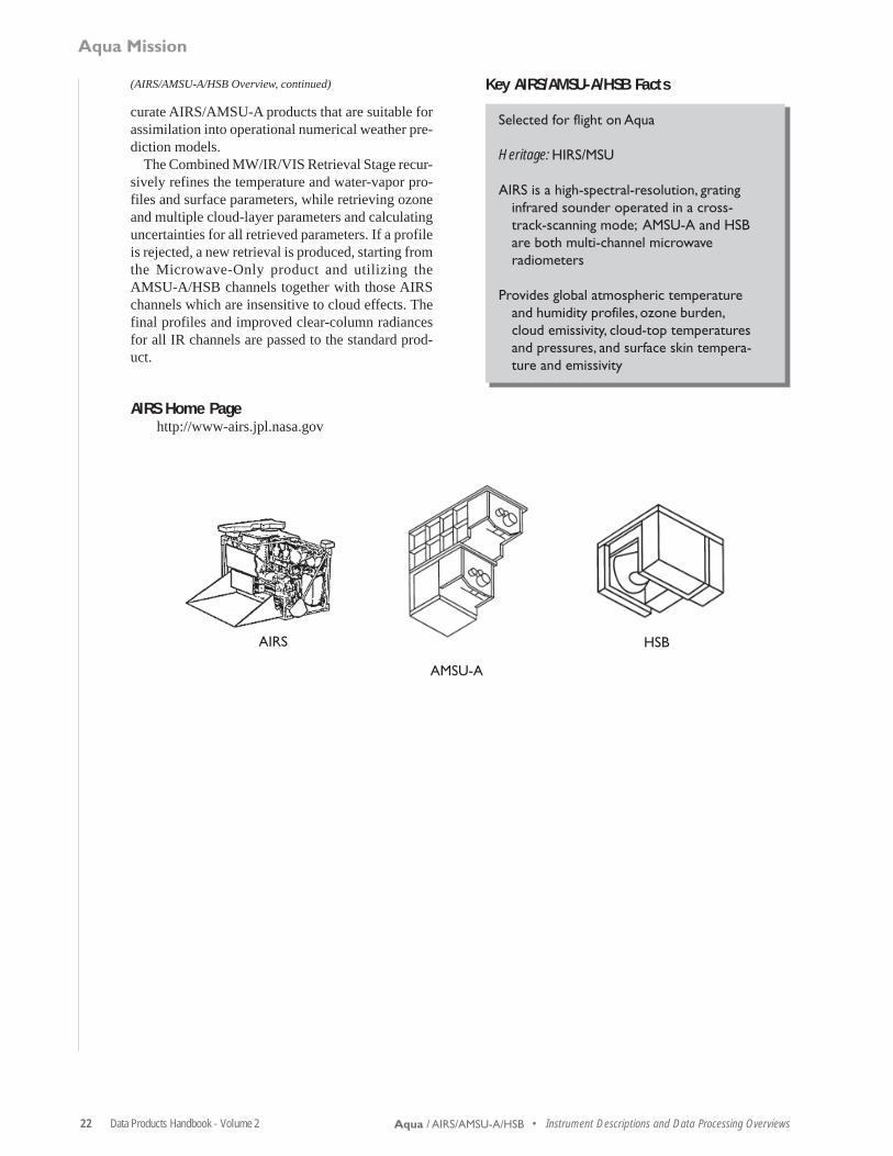
AIRS/AMSU-A/HSB• Atmospheric InfraRed Sounder (AIRS)• Advanced Microwave Sounding Unit (AMSU-A)• Humidity Sounder for Brazil (HSB)
AIRS is a high-resolution infrared (IR) sounder se-lected to fly on the EOS Aqua platform with two op-erational microwave sounders, AMSU-A and HSB.Measurements from the three instruments will beanalyzed jointly to filter out the effects of clouds fromthe IR data in order to derive clear-column air-tem-perature profiles and surface temperatures with highvertical resolution and accuracy. Together, these threeinstruments constitute an advanced operationalsounding system whose data will:
a) improve global modeling efforts and numericalweather prediction;
b) enhance studies of the global energy and watercycles, the effects of greenhouse gases, and at-mosphere-surface interactions; and
c) facilitate monitoring of climate variations andtrends.
AIRS measures upwelling radiances in 2378 spec-tral channels covering the IR spectral band, 3.74 mi-crometers to 15.4 micrometers. A set of four chan-nels in the visible/Near-IR (VIS) observeswavelengths from 0.4 to 1.0 micrometers to providecloud cover and spatial-variability characterization.The microwave sounders provide sea ice concentra-tion, snow cover, and additional temperature-profileinformation as well as precipitable water and cloudliquid-water content. If cloud cover is too great forIR retrievals, the microwave (MW) measurementsalone will provide a coarse, low-precision atmo-spheric-temperature profile and surface characteriza-tion.
The figure on page 23 provides an overview of thedata processing architecture and the products whichoriginate at the various stages.
Three independent Product Generation Executives(PGEs), one each for AIRS/VIS, AMSU-A, and HSB,execute at the DAAC to ingest Level 0 data to pro-duce Level 1A geolocated science data counts andengineering parameters in Hierarchical Data Format(HDF) swath format.
Four independent PGEs, one for each instrument,execute at the DAAC to ingest Level 1A data to pro-duce a Level 1B calibrated IR radiance product, amicrowave brightness temperature product, and as-sociated calibration coefficients. The AIRS L1B PGEalso produces a subset data file of selected cloudy IRradiances for ingest by the AIRS L1B daily browse
PGE. The AIRS and AMSU-A/HSB L1B dailybrowse PGEs subsequently produce browse productsfrom this subset file and the L1B brightness tempera-ture product data.
A combined AIRS/AMSU-A/HSB/VIS Level 2PGE executes at the DAAC to ingest the Level 1Bdata products and ancillary data and to produceLevel 2 standard products and support products, allin HDF swath format. A Level 2 subset data file isalso produced for ingest by the Level 2 daily browsePGE. This daily browse PGE produces browse prod-ucts from this subset file as well as summary data tobe ingested by follow-on Level 2 pentad and Level 2monthly browse PGEs. All browse PGEs are executedat the DAAC.
Quality Assurance (QA) Support Products are pro-duced at the Team Leader Science Computing Facil-ity (TLSCF) in HDF swath format for a fraction ofthe total data set and are used to monitor the opera-tion of the instrument and validate the retrieval algo-rithm and products.
The microwave Level 1B data sets and Level 2standard products are ingested at the TLSCF alongwith the ancillary radiosonde observations (RAOBS)to produce a daily statistic by comparison of profilesobserved by radiosondes with spatially and tempo-rally matched retrieval profiles.
The combined Level 2 PGE consists of three ma-jor retrieval stages:
• Microwave-Only Retrieval• Cloud Clearing• Combined MW/IR/VIS Retrieval
The Microwave-Only Retrieval employs only theAMSU-A and HSB data in combination with an an-cillary general circulation model (GCM) (providinggeneral climatology and accurate surface pressure)and a digital elevation model (DEM) (providing to-pography and land/water fractions) to retrieve atmo-spheric temperature, water vapor, and liquid-waterprofiles as well as surface skin temperature and mi-crowave spectral surface emissivity. A rain flag is alsoproduced. These profiles are passed to the combinedMW/IR/VIS retrieval as an initial guess. In the eventof rain or overwhelming cloud cover, the combinedretrieval is not attempted and the MW-Only Retrievalis passed through to the standard product.
The Cloud Clearing Stage employs MW and se-lected IR channels to estimate the clear-column IRradiances for all IR channels. It also employs IR win-dow channels to retrieve the surface skin tempera-ture, emissivity, and reflectivity. The temperature andwater-vapor profiles are corrected for the effects ofthe clouds. This rapid stage produces reasonably ac-
Aqua / AIRS/AMSU-A/HSB
Aqua Mission
22 Data Products Handbook - Volume 2 • Instrument Descriptions and Data Processing Overviews
curate AIRS/AMSU-A products that are suitable forassimilation into operational numerical weather pre-diction models.
The Combined MW/IR/VIS Retrieval Stage recur-sively refines the temperature and water-vapor pro-files and surface parameters, while retrieving ozoneand multiple cloud-layer parameters and calculatinguncertainties for all retrieved parameters. If a profileis rejected, a new retrieval is produced, starting fromthe Microwave-Only product and utilizing theAMSU-A/HSB channels together with those AIRSchannels which are insensitive to cloud effects. Thefinal profiles and improved clear-column radiancesfor all IR channels are passed to the standard prod-uct.
AIRS Home Pagehttp://www-airs.jpl.nasa.gov
AIRS
AMSU-A
HSB
Key AIRS/AMSU-A/HSB Facts
Selected for flight on Aqua
Heritage: HIRS/MSU
AIRS is a high-spectral-resolution, gratinginfrared sounder operated in a cross-track-scanning mode; AMSU-A and HSBare both multi-channel microwaveradiometers
Provides global atmospheric temperatureand humidity profiles, ozone burden,cloud emissivity, cloud-top temperaturesand pressures, and surface skin tempera-ture and emissivity
(AIRS/AMSU-A/HSB Overview, continued)
Aqua / AIRS/AMSU-A/HSB
Aqua Mission

Data Products Handbook - Volume 2 23Instrument Descriptions and Data Processing Overviews • Aqua / AIRS/AMSU-A/HSB
Aqua Mission
AIRS/AMSU-A/HSB Data Processing Architecture and Products
Leve
l 0
EngineeringArchivalProduct
Daily Browse Product(HDF Format) Daily Browse Product
(HDF Format)
Daily Browse Product
(HDF Format)
Pentad/Monthly Browse Products
(HDF Format)
SupportProducts
(HDF Swath)
QA SupportProducts
(HDF Swath)
Statistics ofMatched Profiles
AIRSL0 Data
VISL0 Data
AIRS/VIS L1A PGE
AMSU-AL0 Data
HSBL0 Data
AMSU-A L1A PGE HSB L1A PGE
Geo-LocatedScience Data Counts andEngineering Parameters(HDF Swath Format)
Geo-LocatedScience Data Counts andEngineering Parameters(HDF Swath Format)
AMSU-A L1B PGE HSB L1B PGE
Calibrated, Geo-Located Brightness Temperatures
and Calibration Coefficients
(HDF Swath Format)
Calibrated, Geo-Located Brightness Temperatures
and Calibration Coefficients
(HDF Swath Format)
AIRS L1B DailyBrowse PGE
AMSU-Aand HSB
L1BProducts
andRAOBS
Daily Stat PGE
Surface Skin Temperature Surface Emissivity
Surface Snow/Ice DetectionRain Flag
Temperature ProfileH2O Vapor and Liquid Profiles
Cloud Cleared IR RadiancesRefined T, H2O Profiles
At TLSCFStandardProducts
(HDF Swath)
Combined AIRS/AMSU-A/HSB/VIS Level 2 PGE
CombinedMW/IR/VIS
Retrieval Stage
Cloud Cleared IR RadiancesSurface Skin T, Emissivity
T, H2O, O3 ProfilesCloud Cover, Emissivity, T, p
Microwave-OnlyRetrieval Stage
Cloud ClearingStage
Geo-LocatedScience Data Counts andEngineering Parameters(HDF Swath Format)
AIRS L1B PGE VIS L1B PGE
AIRS L1B Subset Data(HDF Swath)
AIRS L1B DailyBrowse PGE
Calibrated, Geo-Located Radiances and Calibration
Coefficients(HDF Swath Format)
Calibrated, Geo-Located Radiances and Calibration
Coefficients(HDF Swath Format)
AncillaryData
GCMDEM
RAOBSTOMS
etc.
L2 Pentad/MonthlyBrowse PGE
L2 Subset Data(HDF Swath)
L2 DailyBrowse PGE
SummaryData
(HDF Swath)
Leve
l 1A
Leve
l 1B
Leve
l 2

24 Data Products Handbook - Volume 2 • Instrument Descriptions and Data Processing OverviewsAqua / AMSR-E
AMSR-EAdvanced Microwave Scanning Radiometer for EOS
AMSR-E will be carried aboard the EOS Aqua satel-lite and will monitor a range of hydrologic processescritical to our knowledge of climate variability. Aunique capability of AMSR-E, versus the other EOSinstruments, is its ability to make most of its mea-surements through cloud cover. Over the ocean, theinstrument will measure rainfall, cloud-water andwater-vapor abundance, sea ice parameters, sea sur-face temperature, and near-surface wind speed. Overland, vegetation amounts, snow cover, and soil wet-ness will be monitored. AMSR-E will provide un-precedented detail and accuracy in the global, all-weather measurement of these variables and therebywill allow a more-complete understanding of climatevariability, ultimately enabling better climate predic-tion.
The instrument is a twelve-channel, six-frequency,total power passive-microwave radiometer system.It measures brightness temperatures at 6.925, 10.65,18.7, 23.8, 36.5, and 89.0 GHz. Vertically and hori-zontally polarized measurements are taken at all chan-nels. The Earth-emitted microwave radiation is col-lected by an offset parabolic reflector 1.6 meters indiameter that scans across the Earth along an imagi-nary conical surface, maintaining a constant Earthincidence angle of 55° and providing a swath widthof 1445 km. The reflector focuses radiation into anarray of six feedhorns which then carry the radiationto radiometers for measurement. Calibration is ac-complished with observations of the cosmic back-ground radiation and an on-board warm target. Spa-tial resolution of the individual measurements variesfrom 5.4 km at 89 GHz to 56 km at 6.9 GHz.
The AMSR-E will provide instantaneous measure-ments for the following data products:
• Rainfall over ocean with an accuracy of 1 mm/hror 20%, whichever is greater, at a spatial resolu-tion of 5.4 km.
• Rainfall over land with an accuracy of 2 mm/hr or40%, whichever is greater, at a spatial resolutionof 5.4 km.
• Sea surface temperature, through most clouds, withan accuracy of 0.5° C at two different spatial reso-lutions: 56 and 38 km.
• Total integrated water vapor over the ocean withan accuracy of 0.2 g/cm2 at a resolution of 24 km.
• Total integrated cloud water over the ocean withan accuracy of 3 mg/cm2 at a resolution of 12 km.
• Ocean surface wind speed with an accuracy of1.5 m/s at two resolutions: 38 and 24 km.
• Surface soil wetness with an accuracy of 0.06 gm/cm3 in low-vegetation areas (biomass less than 1.5kg/m2), at a spatial resolution of 25 km.
• Sea ice concentration at two resolutions (SSM/Igrid): 12.5 and 25 km.
• Snow depth over sea ice at a resolution of 12.5 km.
• Sea ice temperature at a resolution of 25 km.
• Snow-cover water equivalent over land.
AMSR-E Home Page: http://www.ghcc.msfc.nasa.gov/AMSR
Key AMSR-E Facts
Selected for flight on EOS Aqua spacecraft
Heritage: Nimbus 7 and Seasat SMMR, DMSPSSM/I
Multi-frequency, dual polarization conicallyscanning passive-microwave radiometer
Measures hydrologic processes
AMSR-E
Aqua Mission

Data Products Handbook - Volume 2 25Instrument Descriptions and Data Processing Overviews •
AMSR-E Standard Products
Aqua / AMSR-E
Aqua Mission
Lev
el 1
*L
evel
2L
evel
3
2A (spatially consistent Tbs)
Ocean Suite:SST
Water vaporCloud waterWind Speed
Brightness Temperatures (Tbs)
Rainfallover land and
ocean, rain type
Azimuthal Equalarea EASE grid
Cylindrical Equal area EASE grid
Surface soilmoisture
Gridded brightnesstemperature (pol. ste.)
Sea Ice Products:ConcentrationTemperature
Snow depth on ice
Ocean SuiteSST
Water vaporCloud waterWind Speed
Monthly rainfall over land and
ocean
Snow waterequivalent
Surface soilmoisture
gridded brightness temperature
* produced by NASDA

26 Data Products Handbook - Volume 2 • Instrument Descriptions and Data Processing OverviewsAqua / CERES
Aqua Mission
CERESClouds and the Earth’s Radiant Energy System
The U.S. Global Change Research Program classi-fies the role of clouds and radiation as its highestscientific priority (CEES, 1994). There are manyexcellent summaries of the scientific issues (IPCC,1992; Hansen et al., 1993; Ramanathan et al., 1989;Randall et al., 1989, Wielicki et al., 1995) concern-ing the role of clouds and radiation in the climatesystem. These issues naturally lead to a requirementfor improved global observations of both radiativefluxes and cloud physical properties. The CERESScience Team, in conjunction with the EOS Investi-gators Working Group representing a wide range ofscientific disciplines from oceans, to land processes,to atmosphere, has examined these issues and pro-posed an observational system with the followingobjectives:
1) For climate-change analysis, provide a continua-tion of the ERBE record of radiative fluxes at thetop of the atmosphere (TOA), analyzed using thesame algorithms that produced the existing ERBEdata.
2) Double the accuracy of estimates of radiativefluxes at TOA and the Earth’s surface.
3) Provide the first long-term global estimates of theradiative fluxes within the Earth’s atmosphere.
4) Provide cloud-property estimates which are con-sistent with the radiative fluxes from the surfaceto the top of the atmosphere.
To accomplish these goals, the CERES data prod-ucts are divided into three major categories, as shownin the figure on the following page: ERBE-like Prod-ucts (top row), CERES Surface/TOA Products(middle row), and CERES Surface/TOA/Atmosphere(bottom row).
The ERBE-like products address the first objec-tive of long-term continuity of the ERBE TOA fluxes.The TOA/Surface Products address the second ob-jective and attempt to provide the most direct tie be-tween surface radiative-flux estimates and TOA fluxmeasurements. The TOA/Surface/Atmosphere prod-ucts focus on the last two objectives and attempt toderive an internally consistent set of atmosphere,cloud, and surface-to-TOA radiative fluxes, all withinthe context of a state-of-the-art radiative-transfermodel. In this last case, the observed TOA fluxes areused as a direct constraint on the model calculations
in order to implicitly account for non-plane-paralleland other poorly modeled atmospheric radiative ef-fects. As in ERBE, CERES radiative fluxes will beseparately determined for both clear- and cloudy-skyconditions.
One of the major advances of CERES over ERBEis the availability of high spatial and spectral resolu-tion cloud imagers for cloud masking, cloud height,and cloud-optical-property determination (i.e., VIRSon TRMM, MODIS on Terra and Aqua). A secondmajor advance is the use of one CERES scanner in across-track mode (global spatial coverage) and a sec-ond scanner in a rotating-azimuth-plane mode (com-plete angular sampling of viewing zenith and azi-muth). The rotating-azimuth-plane scanner data willbe combined with nearly simultaneous cloud-imagerdata to develop a new set of improved empiricalmodels of the SW and LW anisotropy of radiation asa function of surface and cloud type. While it is esti-mated to take two years of these data to develop newangular models, they are expected to reduce instan-taneous TOA flux errors by a factor of three from theERBE levels.
A detailed listing of the CERES data products andtheir individual parameters can be found in theCERES Data Products Catalog (http://asd-www.larc.nasa.gov/DPC/DPC.html). Documentationof the Release 1 CERES analysis algorithms can befound in the CERES Algorithm Theoretical BasisDocuments (ATBDs) Volumes 0 through 12, whereeach volume covers one of the CERES Data Prod-ucts and its associated technical algorithms (http://eospso.gsfc.nasa.gov/atbd/cerestables.html). A sum-mary of the CERES experiment can be found inWielicki et al., Bulletin of the American Meteoro-logical Society, May, 1996.
CERES Home Pagehttp://asd-www.larc.nasa.gov/ceres/docs.html

Data Products Handbook - Volume 2 27Instrument Descriptions and Data Processing Overviews •
Key CERES Facts
Selected for flight on TRMM, Terra, and Aqua
Heritage: ERBE
Broadband, scanning radiometer capable ofoperating in cross-track mode, or rotatingplane mode (bi-axial scanning)
Measures Earth’s radiation budget andatmospheric radiation from the top of theatmosphere to the surface
First instrument (cross-track scanning) willessentially continue the ERBE mission; thesecond (biaxially scanning) will provideangular radiance information that willimprove the accuracy of angular modelsused to derive the Earth’s radiativebalance
Dual scanners on Aqua
CERES
CERES Data Processing Architecture and Products
Aqua / CERES
Aqua Mission
BDS
Level 1Geolocated
Radiance
ES-8
Level 2ERBE-like Instantaneous
TOA Estimates
ES-4. ES-9
Level 3ERBE-like Monthly
Averages
SSF
Level 2Single Scanner TOA/Surface Fluxes and
Clouds
CRS
Level 2Clouds and
Radiative Swath
FSW
Level 3Monthly GriddedRadiative Fluxes
and Clouds
SYN
Level 3Synoptic RadiativeFluxes and Clouds
AVG, ZAVG
Level 3Monthly Regional, Zonal,
and Global Radiative Fluxes and Clouds
SFC
Level 3Monthly Gridded
TOA/Surface Fluxes and Clouds
SRBAVG
Level 3Monthly TOA/
Surface Averages
ER
BE
-Lik
eS
urfa
ce/T
OA
Sur
face
/TO
A/
Atm
osp
here

28 Data Products Handbook - Volume 2 • Instrument Descriptions and Data Processing OverviewsAqua / MODIS
Aqua Mission
MODIS Moderate Resolution Imaging Spectroradiometer
MODIS is an EOS facility instrument designed tomeasure biological and physical processes on a glo-bal basis every one to two days. Slated for both theTerra and Aqua satellites, the instrument will pro-vide long-term observations from which to derive anenhanced knowledge of global dynamics and pro-cesses occurring on the surface of the Earth and inthe lower atmosphere. This multidisciplinary instru-ment will yield simultaneous, congruent observationsof high-priority atmospheric (cloud cover and asso-ciated properties), oceanic (sea-surface temperatureand chlorophyll), and land-surface features (land-cover changes, land-surface temperature, and veg-etation properties). The instrument is expected tomake major contributions to the understanding of theglobal Earth system, including interactions betweenland, ocean, and atmospheric processes.
The MODIS instrument employs a conventionalimaging-radiometer concept, consisting of a cross-track scan mirror and collecting optics, and a set oflinear detector arrays with spectral interference fil-ters located in four focal planes. The optical arrange-ment will provide imagery in 36 discrete bands from0.4 to 14.5 µm, selected for diagnostic significancein Earth science. The spectral bands will have spatialresolutions of 250 m, 500 m, or 1 km at nadir; sig-nal-to-noise ratios of greater than 500 at 1-km reso-lution (at a solar zenith angle of 70°); and absoluteirradiance accuracies of ±5 percent from 0.4 to 3 µm(2 percent relative to the Sun) and 1 percent or betterin the thermal infrared (3 to 14.5 µm). MODIS in-struments will provide daylight reflection and day/night emission spectral imaging of any point on theEarth at least every two days, operating continuously.
Many MODIS products are made over time inter-vals ranging from about one week to a month or aseason. These products will be better suited for useby investigators interested in seasonal phenomena.In some cases these products are made to reduce datavolume; in others they are made to provide cloud-free coverage within a defined time period. Becausethe ground track of the EOS spacecraft follows a 16-day repeat cycle, and because there may be biases inthe multiday data sets based on viewing geometry atspecific locations, the MODIS “week” has been de-fined as an 8-day period. The land and ocean dataproducts are based upon 8-day weeks beginning onJanuary 1 of each year. The atmosphere products arealso based on 8-day weeks, but these begin with the
first 8-day period of the Aqua MODIS sensor that isconcurrent with the Terra MODIS schedule and runin an unbroken sequence thereafter. Thus, the landand ocean weeks will not, in general, coincide withthe atmosphere weeks.
MODIS will provide specific global data products,which include the following:
• Surface temperature with 1-km resolution, day andnight, with absolute accuracy of 0.2 K for oceansand 1 K for land;
• Ocean color, defined as ocean-leaving spectral ra-diance within 5 percent from 415 to 653 nm, en-abled by atmospheric correction from near-infra-red sensor channels;
• Chlorophyll fluorescence within 50 percent at sur-face-water concentrations of 0.5 mg m-3;
• Concentrations of chlorophyll a within 35%;
• Vegetation/land-surface cover, conditions, and pro-ductivity
– Net primary productivity, leaf-area index, andintercepted photosynthetically active radiation
– Land cover type, with change detection and iden-tification
– Vegetation indices corrected for atmosphere, soil,and directional effects;
• Snow cover and sea ice cover;
• Land-surface reflectance (atmospherically cor-rected) with bidirectional reflectance and albedo;
• Cloud cover with 250-m resolution by day and1,000-m resolution at night;
• Cloud properties characterized by cloud-dropletphase, optical thickness, droplet size, cloud-toppressure, and emissivity;
• Aerosol properties defined as optical thickness, par-ticle size, and mass transport;
• Fire occurrence, size, and temperature;
• Global distribution of precipitable water; and
• Cirrus-cloud cover.

Data Products Handbook - Volume 2 29Instrument Descriptions and Data Processing Overviews •
The data-product descriptions in the main part of thishandbook refer to MODIS spectral bands by num-ber. These are all defined in the table on the follow-ing page.
MODIS Home Pagehttp://ltpwww.gsfc.nasa.gov/MODIS/MODIS.html
Key MODIS Facts
Selected for flight on Terra and Aqua missions
Heritage: AVHRR, HIRS, Landsat TM, andNimbus 7 CZCS
Medium-resolution, multi-spectral, cross-track-scanning radiometer
Measures biological and physical processes
MODIS
Aqua / MODIS
Aqua Mission

30 Data Products Handbook - Volume 2 • Instrument Descriptions and Data Processing OverviewsAqua / MODIS
Aqua Mission
Center PixelPrimary Use Band Wavelength Bandwidth Size Ltyp SNR @ Ltyp
(nm) (nm) (m)
Land/Cloud/Aerosol 1 645.0 48.0 250 21.8 129.0Boundaries 2 856.5 38.4 250 24.7 200.8
Land/Cloud/Aerosol 3 465.6 18.8 500 35.3 243.4Properties 4 553.6 19.8 500 29.0 228.3
5 1241.6 24.0 500 5.4 74.06 1629.1 28.6 500 7.3 270.47 2114.1 55.7 500 1.0 111.1
Ocean Color/ 8 411.3 14.8 1000 44.9 880.4Phytoplankton/ 9 442.0 9.7 1000 41.9 838.0Biogeochemistry 10 486.9 10.6 1000 32.1 802.5
11 529.6 12.0 1000 27.9 754.112 546.8 10.3 1000 21.0 750.013 665.5 10.1 1000 9.5 913.514 676.8 11.3 1000 8.7 1087.515 746.4 9.9 1000 10.2 600.016 866.2 15.5 1000 6.2 516.7
Atmospheric 17 904.0 35.0 1000 10.0 166.7Water Vapor 18 935.5 13.6 1000 3.6 57.1
19 935.2 46.1 1000 15.0 250.0
Cirrus Clouds 26 1383.0 35.0 1000 6.0 150.0
Center PixelWavelength Bandwidth Size SNR @ Ltyp =
Primary Use Band (µm) (µm) (m) Ltyp(Ttyp) Ltyp/NE L
Surface/Cloud 20 3.785 .19 1000 0.45(300K) 900.0
Temperature 21 3.990 .08 1000 2.38(335K) 203.422 3.970 .09 1000 0.67(300K) 837.523 4.056 .09 1000 0.79(300K) 987.5
Atmospheric 24 4.472 .09 1000 0.17(250K) 141.7Temperature 25 4.545 .09 1000 0.59(275K) 453.8
Water Vapor 27 6.752 .25 1000 1.16(240K) 252.228 7.334 .33 1000 2.18(250K) 641.2
Cloud Properties 29 8.518 .35 1000 9.58(300K) 2661.1
Ozone 30 9.737 .30 1000 3.69(250K) 444.6
Surface/Cloud 31 11.017 .54 1000 9.55(300K) 2808.8Temperature 32 12.032 .52 1000 8.94(300K) 1824.5
Cloud Top 33 13.359 .31 1000 4.52(260K) 452.0Altitude 34 13.675 .33 1000 3.76(250K) 298.4
35 13.907 .33 1000 3.11(240K) 220.636 14.192 .29 1000 2.08(220K) 106.7
SNR = Signal-to-Noise RatioNE = Noise EquivalentLtyp (in W/m2-µm-sr) = Spectral radiance at typical conditions for this productTtyp = Temperature at typical conditions for this product
MODIS Spectral Band Properties

Data Products Handbook - Volume 2 31Instrument Descriptions and Data Processing Overviews •
MODIS Data Processing Architecture and Products, general
Aqua / MODIS
Aqua Mission
Lev
el 1
MODIS Processing
MOD 02Calibrated L1B Radiances
MOD 03Geolocation Data Set
Lev
el 0
MOD 01Level 1A
Lev
el 2
/Lev
el 2
Gri
dded
(L
2G)
MOD 07• Total Ozone Burden
• Stability Indices
• Temperature and Moisture Profiles
• Precipitable Water (IR)
Grid PointerL2G Land
Pointer Files
MOD 35Cloud Mask
MOD 02 MOD 03
MOD 02, MOD 03, MOD 07, MOD 35, Grid Pointer, Grid Angular
Level 1, Level 2 Atmosphere, Level 2 Ocean, Grid Angular, Grid Pointer
Ocean Color (see Oceans Chart)
Ocean Color(L3 prior 8-day period)
MOD 28Sea Surface
Temperature
(L3 prior 8-day period)
Grid AngularL2G Land
Angular Data
L2, L2G, L3, Legend:
MOD 04Aerosol Product
MOD 06Cloud Product
Instrument Packet Data
MOD 02, MOD 03, MOD 04, MOD 07, MOD 35, Grid Pointer, Grid Angular
Oceans
Land
Atmos
Snow Cover(L3 prior 8-day period)
MOD 10 MOD 05Precipitable Water
MOD 28Sea Surface Temperature MOD 11
L2G Land Temperature
MOD 10
(L3 prior 8-day period)
MOD 43
(16-day)BRDF/Albedo
Snow Cover

32 Data Products Handbook - Volume 2 • Instrument Descriptions and Data Processing OverviewsAqua / MODIS
Aqua Mission
MODIS Data Processing Architecture and Products, general (continued)
MOD 28Sea Surface
Temperature(1-, 8-, 24-day,
monthly, yearly)
MOD 27Ocean Productivity
(8-day, yearly)
Ocean Color(1-, 8-, 24-day,monthly, yearly)
MODIS Processing(Continued)
Lev
el 2
Gri
dded
(L
2G)
MOD 08
L3 AtmosphereProducts
(1-, 8-day, monthly)
Lev
el 3
Lev
el 4
MOD 43BRDF/Albedo
(16-day)
MOD 10Snow Cover(1-, 8-day)
MOD 13Vegetation
Indices (8-, 16-day,monthly)
MOD 12Land Cover
Type(96-day)
MOD 11Land SurfaceTemp. & Emis.
(8-day, monthly)
MOD 13Vegetation
Indices
MOD 12Land Cover Type
(L3 prior period orat-launch)
MOD 11(L3 prior period)
MOD 10Snow Cover
MOD 11Land Surface
Temp. & Emis.
MOD 09Surface
Reflectance
MOD 29Sea Ice Cover
Level 2 Atmosphere, Level 2 Ocean, Level 2G Land
MOD 17Vegetation Production (8-day, yearly)
MOD 16
Evapotranspiration (8-day, yearly)
MOD 15LAI and FPAR
(1-, 8-day)
MOD 29Sea Ice Cover
(1-, 8-day)
MOD 14Thermal Anomalies(1-, 8-day, monthly)
MOD 43
(L3 prior period)
Level 1, Level 2 Atmosphere, Level 2 Ocean , L2G Grid Pointer, L2G Grid Angular
MOD 12
(L3 prior period orat-launch)
MOD 44
(L4)
MOD 14Thermal
Anomalies
MOD 44Vegetation Cover
Conversion(3-month. yearly)
MOD 40Burn Scars(8-, 16-day, monthly)
L2, L2G, L3, Legend:
Oceans
Land
Atmos
BRDF/Albedo
Land Cover Type
Vegetation CoverConversion
Surface Resistance and

Data Products Handbook - Volume 2 33Instrument Descriptions and Data Processing Overviews •
MODIS Data Processing Architecture and Products, land
Aqua / MODIS
Aqua Mission
MODIS Land Processing
MOD 09Surface Reflectance
MOD 13Vegetation Indices
MOD 14Thermal Anomalies
MOD 05Precipitable
Water
MOD 35Cloud Mask
MOD 04Aerosol Product
MOD 29Sea Ice Cover
MOD 10Snow Cover
Lev
el 2
Gri
dded
(L
2G)
Lev
el 1
MOD 02Calibrated L1B Radiances
MOD 03Geolocation Data Set
Instrument Packet Data
Lev
el 0
MOD 01Level 1A
MOD 02, Grid Pointer, Grid Angular
MOD 11Land SurfaceTemp. & Emis.
MOD 35Cloud Mask
Level 2G
MOD 43BRDF/Albedo
(16-day)
MOD 10Snow Cover(1-, 8-day)
MOD 13Vegetation Indices
(8-, 16-day, monthly)
MOD 12Land Cover Type
(96-day)
MOD 11Land SurfaceTemp. & Emis.
(8-day, monthly)
MOD 17Vegetation Production
(8-day, yearly)
MOD 16Surface Resistance and
Evapotranspiration(8-day, yearly)
MOD 15LAI and FPAR
(1-, 8-day)
MOD 29Sea Ice Cover
(1-, 8-day)
MOD 14Thermal Anomalies(1-, 8-day, monthly)
Lev
el 3
Lev
el 4
Grid PointerProduct
Grid AngularData Product
MOD 12 Land Cover Type
(L3 prior period orat-launch)
MOD 11(L3 prior period)
MOD 12(L3 prior period or
at-launch)
MOD 43BRDF/Albedo
(L3 prior period)
MOD 43BRDF/Albedo(Prior period)
MOD 44Vegetation Cover
Conversion (3-month, yearly)
MOD 40Burn Scars(8-, 16-day, monthly)
MOD 04AerosolProduct
MOD 44Vegetation CoverConversion (L4)

34 Data Products Handbook - Volume 2 • Instrument Descriptions and Data Processing OverviewsAqua / MODIS
Aqua Mission
MODIS Data Processing Architecture and Products, atmosphere
Lev
el 1 MOD 02
Calibrated L1B Radiances
MOD 03Geolocation Data Set
Lev
el 0
MOD 01Level 1A
MOD 02 MOD 03
Lev
el 2
MOD 07Atmospheric Profiles
• Total Ozone Burden
• Stability Indices
• Temperature and Moisture Profiles
• Precipitable Water (IR)
MOD 35
Cloud Mask
MODIS Atmosphere Processing
MOD 06Cloud Product
• Cloud Top Properties (temperature, height, emissivity)
• Cloud Particle Phase
• Cloud Fraction
• Cloud Optical Properties (optical thickness and particle size)
Lev
el 3
MOD 03, Level 2 Atmosphere Products
MOD 02, MOD 03, MOD 07, MOD 35
MOD 08L3 Atmosphere Products
• Aerosol • Water Vapor• Clouds • Stability Indices• Ozone
(1-, 8-day, monthly)
Instrument Packet Data
MOD 05Precipitable
Water Product
• Solar Algorithm
• IR Algorithm
MOD 04 Aerosol Product
• Aerosol Optical Thickness
• Aerosol Size Distribution
MOD 11
MOD 10
L2G Land Temperature
Snow Cover(L3 prior 8-day period)
MOD 43BRDF/Albedo
(16-day)
MOD 28Sea Surface Temperature
(L3 prior 8-day period)
MOD 10Snow Cover
(L3 prior 8-dayperiod)

Data Products Handbook - Volume 2 35Instrument Descriptions and Data Processing Overviews •
MODIS Data Processing Architecture and Products, oceans. A complete set of these products will be produced for both Terra andAqua MODIS sensor data. In addition, a merged Terra/Aqua MODIS Ocean product set will be produced at Levels 3 and 4 in the post-Aqua launch period.
Aqua Mission
Aqua / MODIS
Lev
el 2
Lev
el 3
Lev
el 4
MODIS Ocean Processing
MOD04
Sea Aerosol Product
MOD 28
Sea SurfaceTemperature
(1-day)
MOD 28Sea Surface
Temperature(1-, 8-, 24-day, monthly, yearly)
MOD 35Cloud Mask
MOD 04AerosolProduct
MOD 27Ocean
Productivity(8-day, yearly)
Ocean Color:MOD 18 Water-Leaving Rad.MOD 19 Pigment Conc.MOD 20 Chlorophyll Fluor.MOD 21 Chlorophyll Conc.MOD 22 PAR/Interim PARMOD 23 Suspended Solids Conc.MOD 24 Organic Matter Conc. MOD 25 Coccolith Conc.MOD 26 Water Attenuation Coef.MOD 31 Phycoerythrin Conc.MOD 36 Absorption CoefficientsMOD 37 Aerosol Optical DepthMOD 39 Clear-Water Epsilon
MOD 05Precip. Water
MOD 28Sea Surface
Temperature(L3 prior
8-day period)
Lev
el 0
Lev
el 1
MOD 02Calibrated L1B Radiances
MOD 03Geolocation Data Set
MOD 01Level 1A
MOD 02 MOD 03
Ocean Color
(1-, 8-, 24-day, monthly, yearly)
Ocean Color
(L3 prior 8-day period)
Instrument Packet Data

36 Data Products Handbook - Volume 2 • Instrument Descriptions and Data Processing OverviewsJason-1 / Poseidon-2/JMR/DORIS
Jason-1 Mission
Poseidon-2/JMR/DORIS
Jason-1 is a follow-on mission to TOPEX/Poseidon(T/P) to continue high-accuracy measurement of thesea surface topography of the world’s oceans. Themission’s measurements will be used to study: 1) theglobal ocean circulation and its variability in rela-tion to climate variability, 2) the global ocean wavefield, and 3) the global radar backscatter in relationto sea state and gas exchange with the atmosphere.The data are organized as sequential records alongthe ground track of the satellite. Each record con-tains all the information regarding the instrument’smeasurements averaged over a period close to onesecond of flight time, including the measurements ofsea surface height, wave height, radar backscattercross-section, and wind speed, along with a host ofauxiliary data, including atmospheric, geophysical,and instrumental corrections as well as other relevantinformation such as ocean-tide model products andatmospheric-pressure products.
The Jason-1 mission was defined in a way that al-lows an optimum continuation of the T/P scientificmission and fulfillment of the long-term observationrequirements. The satellite is designed for a mini-mum duration of three years, with a potential for anadditional two years. Every 10 days, it will overflywithin 1 km the reference T/P ground-tracks (66° in-clination, 1336 km orbit), measuring sea level withthe same or better accuracy than T/P. The Jason-1payload includes a similar package as for T/P. CNES(Centre National d’Etudes Spatiales) provides thePoseidon-2 altimeter, which is a solid-state, low-power-consumption, low-mass instrument. It is de-rived from the Poseidon-1 altimeter of T/P but worksat two frequencies (13.6 GHz and 5.3 GHz) to en-able an ionospheric correction accuracy in accordancewith the required error budget. The DORIS PreciseOrbit Determination system, whose ultimate perfor-mance has been demonstrated on T/P, is also pro-vided by CNES. JPL/NASA is responsible for de-veloping the 3-frequency Jason-1 MicrowaveRadiometer (JMR) which will be used to computethe troposphere path-delay correction with the re-quired accuracy. A TurboRogue Space GPS Receiverand a Laser Retroreflector Array, also provided byJPL/NASA, will contribute to the Precise Orbit De-termination effort. The US Delta II vehicle will beused to launch the Jason-1 satellite, jointly with theTIMED satellite, from the Vandenberg Air ForceBase.
The raw engineering Jason-1 data will be recordedon board the satellite, then transmitted to the ground
when over-flying the two main telemetry stationslocated in Aussagel (near Toulouse, France) and inPoker-Flat (Alaska). One backup station is locatedat the Wallops Flight Facility in Virginia. In additionto these Earth terminals, the control ground systemwill include a Satellite Control Center located inCNES and a Project Operation Control Center(POCC) at JPL. The mission ground system will beresponsible for instrument programming/monitoringas well as scientific product generation and distribu-tion. It will comprise: 1) a CNES center calledSSALTO (Segment Sol Multimission Altimetry andOrbitography), which will work not only for Jason-1, but also for other DORIS missions and the Envisataltimeter mission, and 2) a NASA center, which ispart of the JPL POCC and derived from the T/Pground system.
The Geophysical Data Records (GDRs) will con-stitute the final and fully validated products. Theywill be systematically delivered to data users within30 days and eventually archived as permanentrecords. They will contain, at a rate of one record persecond, the best estimates of range measurement, thetime tag and Earth location, plus the best associatedinstrumental and environmental corrections and themost accurate orbit altitude. All these parameters willbe validated during the verification phase of the mis-sion, covering the first 6-8 months after launch. TheGDR, structured in a way similar to what has beenused with T/P, will contain the following additionalgeophysical parameters: wave-height, sigma-naughtand derived wind speed, atmospheric surface pres-sure, tides, mean sea surface, and the geoid. The al-timeter radar instrument bias and drift and the rela-tive bias between T/P and Jason-1 time series will beprovided. For specific applications (over ocean,coastal areas, lake, land, or ice), the Sensor Geophysi-cal Data Records (SGDR), containing waveforms,will be made available to users.
The Interim GDRs (IGDRs) and Operational Sen-sor Data Records (OSDR) will support near-real-timeapplications, including mesoscale and coastal appli-cations, climate forecasting, and marine meteorol-ogy. Wind speed, significant wave-height (SWH), andtheir forecasts are of interest to many activities re-lated to maritime industries. The key requirement foroperational use of altimetric data in models is to pro-vide the data within a very short time period. IGDRswill be delivered within three days, mainly for me-soscale and climate applications. They will containthe same parameters as GDRs, but not fully validatedand not necessarily in their ultimate precision. OSDRswill be provided within three hours, mainly for sup-porting marine meteorology applications. They will

Data Products Handbook - Volume 2 37Instrument Descriptions and Data Processing Overviews •
contain, at a rate of one record per second, all param-eters needed for such applications. OSDR productswill have a lower accuracy than IGDR products, asthey are based on on-board processing for radar al-timetry and orbit determination (DORIS navigator).SWH and wind speed will have respective accuraciesof 10% or 0.5 m (whichever is greater) and 2 m/s.
Jason-1 Home Pagehttp://topex-www.jpl.nasa.gov/jason1/
Jason-1
Key Poseidon-2/JMR/DORIS Facts
Selected for flight on Jason-1
Heritage: Poseidon-1, TMR, and DORIS onTOPEX/Poseidon
Poseidon-2 is a dual-frequency solid-stateradar altimeter (13.6 GHz and 5.3 GHz);JMR is a 3-frequency microwave radiom-eter; DORIS is a 2-frequency receivermeasuring signals received from ground-based beacons
Provides high-accuracy global observationsof ocean topography, wave height, andwind speed, plus, from the JMR, columnarwater vapor content and, fromPoseidon-2, total electron content
Jason-1 / Poseidon-2/JMR/DORIS
Jason-1 Mission

38 Data Products Handbook - Volume 2 • Instrument Descriptions and Data Processing Overviews
ETM+Enhanced Thematic Mapper Plus
The Enhanced Thematic Mapper Plus (ETM+) hasflown on the Landsat 7 satellite as of 15 April 1999,and provides synoptic, repetitive, multispectral, high-resolution, digital imagery of the Earth’s land sur-faces. Since 1972, the Landsat Program has providedcalibrated land-surface digital imagery to a broad usergroup including the agricultural community, globalchange researchers, state and local governments,commercial users, international users, and the mili-tary. The Landsat 7 mission will extend the databaseof the Earth’s surface into the next century.
The ETM+ instrument is an improved version ofthe Thematic Mapper instruments that flew on Land-sat 4 and 5. Like the earlier instruments, the ETM+will acquire data for six visible, near-infrared, andshortwave infrared spectral bands at a spatial resolu-tion of 30 meters.
The ETM+ instrument also incorporates a 15-meterresolution panchromatic band as well as improvedground resolution for the thermal infrared band (60m vs. 120 m). Incorporation of in-flight full- and par-tial-aperture solar calibration will improve the over-all radiometric accuracy to 5 percent. The ETM+ willprovide data that are sufficiently consistent in termsof acquisition geometry, spatial resolution, spectralcharacteristics, and calibration with previous Land-sat data to meet requirements for global change re-search.
The Landsat 7 satellite operates in a circular, sun-synchronous orbit with an inclination of 98.2°, analtitude of 705 km, and a descending node equatorialcrossing time of 10:00 AM plus or minus 15 min-utes. This orbit allows Landsat 7 to precede the Terrasatellite by 30 minutes along a common ground track.The 185 km swath of coverage provided by the ETM+field-of-view affords a global view every 16 days.
ETM+ data will be used primarily to characterizeand monitor change in land cover and land-surfaceprocesses. The high spatial resolution and seasonalglobal coverage of ETM+ will allow improved as-sessment of both the rates of land cover change, andthe local processes responsible for those changes. De-forestation, ecosystem fragmentation, agriculturalproductivity, glacier dynamics, coastal hazards, andvolcano monitoring are all science targets for ETM+.The common orbit with Terra offers additional op-portunities for data fusion with the data from theASTER, MISR, and MODIS sensors.
The mission will generate and periodically refresha global archive with substantially cloud-free, sunlitdata. To facilitate this objective, a long-term acquisi-tion plan has been devised to ensure maximal globaldata acquisition, taking into account vegetation sea-sonality, cloud cover, and instrument gain.
Data stored on board, as well as real-time conti-nental U.S. data, will be downlinked to the Landsat 7ground station located at the EROS Data Center(EDC) in South Dakota. Data received at the EDCwill be processed for archiving and distribution bythe Land Processes DAAC. All data received at EDCwill be available at L0R (no radiometric calibration;limited geometric correction). In addition, a subsetof these scenes can be processed to Level 1 (radio-metric and geometric corrections applied).
ETM+/Landsat Home Pagehttp://landsat.gsfc.nasa.gov/
Key ETM+ Facts
Selected for flight on Landsat 7, launchedApril 15, 1999
Heritage: Landsat 4, 5 and 6
Imaging radiometer with 7 spectral bands fromvisible to thermal infrared plus a panchro-matic band; 16-day repeat cycle
Provides high spatial resolution, multispectralimages of the sunlit land surface
Landsat 7
Landsat 7 / ETM+
Landsat 7 Mission
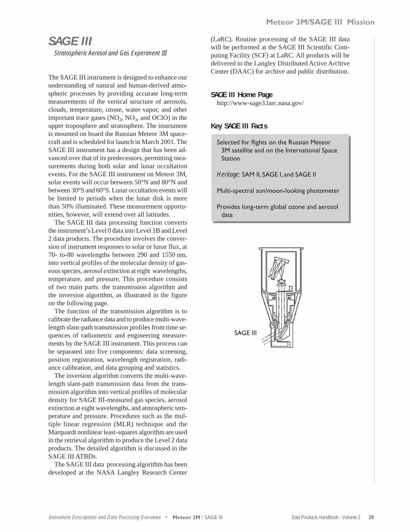
Data Products Handbook - Volume 2 39Instrument Descriptions and Data Processing Overviews • Meteor 3M / SAGE III
SAGE IIIStratospheric Aerosol and Gas Experiment III
The SAGE III instrument is designed to enhance ourunderstanding of natural and human-derived atmo-spheric processes by providing accurate long-termmeasurements of the vertical structure of aerosols,clouds, temperature, ozone, water vapor, and otherimportant trace gases (NO2, NO3, and OClO) in theupper troposphere and stratosphere. The instrumentis mounted on board the Russian Meteor 3M space-craft and is scheduled for launch in March 2001. TheSAGE III instrument has a design that has been ad-vanced over that of its predecessors, permitting mea-surements during both solar and lunar occultationevents. For the SAGE III instrument on Meteor 3M,solar events will occur between 50°N and 80°N andbetween 30°S and 60°S. Lunar occultation events willbe limited to periods when the lunar disk is morethan 50% illuminated. These measurement opportu-nities, however, will extend over all latitudes.
The SAGE III data processing function convertsthe instrument’s Level 0 data into Level 1B and Level2 data products. The procedure involves the conver-sion of instrument responses to solar or lunar flux, at70- to-80 wavelengths between 290 and 1550 nm,into vertical profiles of the molecular density of gas-eous species, aerosol extinction at eight wavelengths,temperature, and pressure. This procedure consistsof two main parts: the transmission algorithm andthe inversion algorithm, as illustrated in the figureon the following page.
The function of the transmission algorithm is tocalibrate the radiance data and to produce multi-wave-length slant-path transmission profiles from time se-quences of radiometric and engineering measure-ments by the SAGE III instrument. This process canbe separated into five components: data screening,position registration, wavelength registration, radi-ance calibration, and data grouping and statistics.
The inversion algorithm converts the multi-wave-length slant-path transmission data from the trans-mission algorithm into vertical profiles of moleculardensity for SAGE III-measured gas species, aerosolextinction at eight wavelengths, and atmospheric tem-perature and pressure. Procedures such as the mul-tiple linear regression (MLR) technique and theMarquardt nonlinear least-squares algorithm are usedin the retrieval algorithm to produce the Level 2 dataproducts. The detailed algorithm is discussed in theSAGE III ATBDs.
The SAGE III data processing algorithm has beendeveloped at the NASA Langley Research Center
(LaRC). Routine processing of the SAGE III datawill be performed at the SAGE III Scientific Com-puting Facility (SCF) at LaRC. All products will bedelivered to the Langley Distributed Active ArchiveCenter (DAAC) for archive and public distribution.
SAGE III Home Pagehttp://www-sage3.larc.nasa.gov/
Key SAGE III Facts
Selected for flights on the Russian Meteor3M satellite and on the International SpaceStation
Heritage: SAM II, SAGE I, and SAGE II
Multi-spectral sun/moon-looking photometer
Provides long-term global ozone and aerosoldata
SAGE III
Meteor 3M/SAGE III Mission

40 Data Products Handbook - Volume 2 • Instrument Descriptions and Data Processing Overviews
SAGE III Data Processing Architecture and Products
Meteor 3M/SAGE III Mission
Meteor 3M / SAGE III
Output Data Products
Profile Inversion
Convergence Test
Temperature andPressure Retrieval
H2O Retrieval
O3, Aerosol Slant-PathCalculations using Least Squares
NO2, O3, Slant-PathCalculations using MLR
NCEPMeteorological Data
Level 0 (Telemetry) DataProcessing
Data Screening
Position Registration(Refraction Correction)
Wavelength Registration
Radiance Calibration(Transmission Calculations)
Data Grouping and Statistics
Transmission
Rayleigh ScatteringCalculations
INVE
RSIO
NTR
ANSM
ISSI
ON

Data Products Handbook - Volume 2 41Instrument Descriptions and Data Processing Overviews • QuikScat / SeaWinds
SeaWinds
The SeaWinds instruments are specialized microwaveradars designed to make moderate-resolution, broad-swath measurements of global radar backscatter andocean-surface wind speed and direction under nearlyall-weather conditions. SeaWinds vector-wind mea-surements are critical for investigating and model-ing upper-ocean circulation, marine meteorologicalprocesses, and large-scale air-sea interaction and cli-mate. The data are provided to the U.S. NationalOceanic and Atmospheric Administration (NOAA)and the EOS Data Assimilation Office (DAO) in near-real-time for use in regional and global weather pre-diction and marine forecasting. NOAA distributesnear-real-time SeaWinds wind-velocity data to inter-national operational weather prediction centers.
The SeaWinds radar backscatter cross-sectionmeasurements over land provide information on veg-etation type and both seasonal and interannualchange. Measurements over continental and sea-ice-covered areas are used to monitor ice extent andfreeze/melt processes on diurnal through interannualtime scales.
SeaWinds is a dual, conically scanning pencil-beamradar operating at 13.4 GHz. Vertically polarizedbackscatter cross-section measurements at ~54° in-cidence angle are acquired over an 1800-km-wideswath centered on the satellite subtrack. Horizontallypolarized data are acquired over a concentric 1400-km-wide swath at ~46° incidence angle. The antennaspins at 18 rpm, yielding measurements with 25-×-35-km IFOV. Modulation of the transmitted pulsesallows extraction of cross-section data with ~6-×-25-km spatial resolution. SeaWinds vector-wind mea-surements are obtained with 25-km resolution acrossnearly the entire swath, and cover more than 90% ofthe global, ice-free oceans daily.
Significant ground processing is required to ex-tract accurate backscatter cross-section and vector-wind measurements from raw SeaWinds radar mea-surements. The surface normalized radar cross-section is calculated from the received power andknowledge of the viewing geometry and instrumentcharacteristics. Over the ocean, backscattering resultsprimarily from centimetric ocean roughness elementswhose amplitudes and directional distributions arein local equilibrium with the local wind. The oceanbackscatter cross-section thus varies with wind speedand direction relative to the radar beam. Vector-windmeasurements are thus obtained by combining mul-tiple, near-simultaneous, collocated backscatter mea-surements acquired from different viewing geom-etries as the satellite passes overhead. SeaWinds
ocean vector-wind products include flags to indicatethe presence of contamination resulting from heavyrain conditions.
Two SeaWinds instruments will be flown in thefirst set of EOS missions. The QuikScat mission, withSeaWinds as the sole science instrument, waslaunched on 19 June 1999 and has been returninghigh-quality data since 19 July 1999. A second Sea-Winds will be launched in late 2001 as part of theNational Space Development Agency (NASDA) ofJapan's ADEOS-II mission; this mission will alsoinclude a broad-swath, multi-channel microwave ra-diometer (an AMSR). A subset of the ADEOS AMSRmeasurements will be used in the ADEOS SeaWindsprocessing to provide atmospheric corrections andadvanced rain flagging to supplement the autonomousSeaWinds flags and to enhance the accuracy of thevector-wind measurements. The figure on the follow-ing page outlines the complete SeaWinds processingchain and standard products.
SeaWinds Homepagehttp://winds.jpl.nasa.gov/
Key SeaWinds Facts
Selected for flights on QuikScat, launchedJune 19, 1999, and the Japanese ADEOS IIsatellite
Heritage: SEASAT, NSCAT
Ku-band scatterometer
Provides near-surface wind velocities overthe oceans, plus information for vegetationclassification and ice-type investigations
QuikScat Mission
SeaWinds onQuikScat

42 Data Products Handbook - Volume 2 • Instrument Descriptions and Data Processing Overviews
Pre-Processors (PP) and Level Processors (LP)SeaWinds Data Flow
SeaWinds L0
SWS L0Raw Telemetry
SWS L1A
UnpackedTelemetry
SWS L1B
BackscatterPower
SWS L2A
Sigma0 w/AMSR
SWS L2BOcean Winds
PP L0:Ingest Telemetry
LP L1A:Convert Telemetry
LP L1B:Calculate Sigma0
LP L2A:Group Sigma0 &
AMSR L1B
LP L2B:Determine Winds &
Flag Rain
ADEOS II AMSR L1A
Convert AMSR 1A toBrightness Temperatures
SeaWinds Data Processing Architecture and Products
QuikScat Mission
QuikScat / SeaWinds

Data Products Handbook - Volume 2 43Instrument Descriptions and Data Processing Overviews • QuikTOMS / TOMS
TOMSTotal Ozone Mapping Spectrometer
The QuikTOMS mission is to continue daily map-ping of the global distribution of the Earth's totalcolumn of atmospheric ozone with the Total OzoneMapping Spectrometer Flight Model 5 (TOMS-FM5). TOMS-FM5 was scheduled to be launched inthe year 2000 aboard a Russian satellite, but thatmission was terminated in April 1999. Because ofthe requirement for monitoring changes in the ozonelayer, NASA had to formulate a new mission to flyTOMS-5 in a very short time. The continuous obser-vation of the global ozone past the year 2000 is criti-cal in order to monitor the expected recovery of ozoneas levels of chlorofluorocarbons (CFCs) decreasefrom their current maximum as a result of theMontreal Protocol limits. The planned three-yearQuikTOMS mission is intended to provide overlapwith the current Earth Probe TOMS, launched in July1996, and with the Ozone Monitoring Instrument(OMI), scheduled for launch on Aura in 2003.
The main objectives of QuikTOMS are: 1) the de-termination of long term change in global total ozonelevel, 2) the understanding of the processes relatedto the “ozone hole” formation and local anomalies inthe equatorial region, and 3) improved understand-ing of processes that govern the generation, deple-tion, and distribution of global total ozone. Additionalobjectives are: the detection and measurement ofvolcanic ash clouds and sulfur dioxide gas, the de-tection and measurement of aerosol and pollutionplumes, and the estimation of surface ultraviolet ir-radiance
TOMS-5 is a f/5 single grating Ebert-Fastie typemonochromator with multiple exit slits for six dif-ferent wavelengths. The nominal center wavelengthvalues of the six bands are 308.6, 312.5, 317.5, 322.3,331.2, 360 nm, and the nominal bandwidth for eachband is 1.2 nm. The wavelength is selected with achopper wheel near the slit plate that gates the pairof the entrance and exit slits for each wavelengthband. The instantaneous field of view (IFOV) ofTOMS-5 is 3° × 3°, which projects to approximately42 km × 42 km at the subsatellite point on the Earthfor the 800 km satellite altitude. TOMS-5 scans ±18scenes from the nadir in a 3° interval to cover ap-proximately 2300 km cross track.
The TOMS instrument records daily global mea-surements of total column ozone, aerosols, Erythe-mal UV exposure, and reflectivity. In the event of a
volcanic eruption it can also measure sulfur dioxidein the eruption plume.
Data are provided in a gridded 1° latitude by 1.25°longitude format. All data processing will be done atthe Science Operations Center at NASA GoddardSpace Flight Center, Greenbelt, Maryland.
QuikTOMS Home Pagehttp://toms.gsfc.nasa.gov/.
Key TOMS Facts
Selected for flights on:Nimbus 7, launched October 24, 1978;Meteor 3, launched August 15, 1991;ADEOS I, launched August 17, 1996;Earth Probe, launched July 2, 1996; andQuikTOMS
Heritage: the earlier TOMS instruments
Six-band monochromator
Provides global daytime measurements oftotal column ozone, aerosols, Erythemalultraviolet exposure, and reflectivity
QuikTOMS Mission

44 Data Products Handbook - Volume 2 • Instrument Descriptions and Data Processing Overviews
QuikTOMS Data Processing Architecture
2 Kbps Uplink400 Kbps Downlink
Satellite Radio Frequency Up/DownFront End ProcessingTemporary Data Storage
EPGN Tracking Stations
Alaska, McMurdo, Norway,Wallops
Tracking Files/DataG/S CommandsS/C CommandsInstrument Commands
S/C TelemetryInstrument DataG/S Status Telemetry
128 Kbps or T1NASA IntegratedServices Network
NASA Central StandardAutonomous File Server
NASA CommunicationsGSFC, MD
256 KbpsPoint-to-Point Circuit
Pass SchedulesS/C TelemetryInstrument DataG/S Status TelemetryPosition Vector
Schedule RequestsS/C EphemerisS/C CommandsInstrument Commands
TOMS Mission ControlCenter
Dulles, VA
FTP(Internet)
InstrumentCommandRequests
Instrument DataAncillary DataS/C EphemerisCommand Request VerificationPass Schedule
TOMS ScienceOperations Center
GSFC, MD
QuikTOMS Mission
QuikTOMS / TOMS

Data Products Handbook - Volume 2 45Instrument Descriptions and Data Processing Overviews • VCL / MBLA
MBLA MultiBeam Laser Altimeter
The Vegetation Canopy Lidar (VCL) is the first se-lected mission of NASA’s new Earth System SciencePathfinder (ESSP) program. The related data prod-ucts listed in this handbook are derived from theMultiBeam Laser Altimeter (MBLA), the instrumentthat will fly on the VCL platform. The principal goalof VCL is the characterization of the three-dimen-sional structure of the Earth: in particular, canopyvertical and horizontal structure and land-surface to-pography. Its primary science objectives are: landcover characterization for terrestrial ecosystem mod-eling, monitoring and prediction; land cover charac-terization for climate modeling and prediction; andproduction of a global reference data set of topo-graphic spot heights and transects. VCL will provideunique data sets for understanding important envi-ronmental issues including climatic change and vari-ability, biotic erosion, and sustainable land use, andwill dramatically improve our estimation of globalbiomass and carbon stocks, fractional forest cover,forest extent and condition. Furthermore, it will pro-vide canopy data critical for biodiversity studies aswell as for natural hazard and climate studies. Sched-uled for launch in late 2000, VCL is an active lidarremote sensing system consisting of a five-beam in-strument with 25-m contiguous along-track resolu-tion. The five beams are in a circular configuration 8km across, and each beam traces a separate groundtrack spaced 2 km apart, eventually producing 2-kmcoverage between 67° N and S latitude. VCL’s coremeasurement objectives are: 1) canopy top heights;2) vertical distribution of intercepted surfaces, e.g.,leaves and branches; and 3) ground-surface topo-graphic elevations. These measurements are used toderive a variety of science data products, includingcanopy heights, canopy vertical distribution, andground elevations gridded at various temporal andspatial resolutions.
The VCL standard data products will be producedby the VCL Data Center (VDC). The VDC consistsof three major science-processing subsystems. Thesescience subsystems are:
• Altimeter Return Echo Analysis System (AREAS)will process the altimeter waveform acquired witheach laser shot. These waveforms will be used todetermine the range to the canopy top and ground,provide information on the Vertical Distributionof Intercepted Surfaces (VDIS), and perhaps de-liver other information, e.g., reflectance, useful inthe characterization of the surface spot being
ranged to. For example, the laser data can be usedto identify water, unvegetated land surfaces, sur-face slopes, terrain roughness, and related infor-mation.
• The VCL Precision Geolocation System (VPGS)will be responsible for providing precise orbitalephemeris information for VCL through the propermodeling of the forces acting on the satellite, re-duction and analysis of the GPS, Satellite LaserRanging (SLR), and laser-altimeter data, and in-corporation of specialized orbit-determinationmethodologies. The system will also utilize the al-timeter ranges acquired over the ocean during timesof special-pointing, off-nadir spacecraft maneuversto derive pointing corrections for the spacecraft’sattitude and laser instrument offsets due to mount-ing and thermal effects, and to geolocate the spoton the surface being ranged to. This orbit-positionand spacecraft-attitude information will be inter-polated to the time of each VCL altimeter range tolocate the surface footprint while retaining the levelof accuracy in the geolocation and pointing solu-tions. The VPGS will also process the raw startracker, gyro, and magnetometer data to provideimproved attitude information in support of thepointing solution.
• The Level 3 Products Generation Subsystem. Thisscience processing system, of less complexity, is agridding package which will generate the mission’sLevel 3 data products, using a variety ofwindowing, averaging, and parsing strategies.
The VDC also supports other important functions,which include:
• Processing data received from telemetry packetsinto various science and intermediate products.This includes unpacking and uncompressing telem-etry to provide gyro/attitude, star tracker, GPS re-ceiver, GPS NAV orbit, and MBLA waveform dataat Level 0.
• Support expedient data delivery (through both asubscription and random ordering capability) andspecialized analysis functions and flexibilityneeded by the Science Team to verify system per-formance, improve processing algorithms, calibrateinstruments, and add value to the processing ap-proaches as the mission evolves.
• Provide all required data and data product distri-bution to the EROS Data Center in Sioux Falls,South Dakota, which is designated as the DAACinterface with the outside science community.
VCL Mission

46 Data Products Handbook - Volume 2 • Instrument Descriptions and Data Processing Overviews
• Provide on-site data archiving, information man-agement, and data-management functions.
• Perform gridding, and visualization functions toassist the Science Team in their evaluation of thesedata and provide interim and final higher level dataproducts for testing and accuracy assessment anddistribution to the EROS Data Center.
• Provide data back-up and security management toprotect the VDC and its data holdings from unau-thorized use and catastrophic failure/events.
• Acquire all data sets in a timely and regular fash-ion externally located from the VDC which areneeded to support AREAS, pointing, and orbit pro-cessing. This includes Earth-orientation informa-tion, solar and magnetic flux, SLR data, snow covergrids, sea state, and like information.
• Provide on-line/near-line access to all subsidiarydata sets which are needed to process, character-ize, and evaluate data products. This includes DEM,urban masks, land/ocean masks, surface-type/char-acterization files, surface-slope masks, etc.
VCL Home Pagehttp://www.inform.umd.edu/geog/vcl
Key MBLA Facts
Selected for flight on VCL, the first mission ofNASA’s ESSP program
Heritage: Shuttle Laser Altimeter (SLA),Mars Orbiter Laser Altimeter (MOLA),Laser Vegetation Imaging Sensor (LVIS)
Laser altimeter system using five, 1064 nm-wavelength lasers in a circular configuration
Measures the three-dimensional structure ofthe Earth, in particular canopy vertical andhorizontal structure and land surface to-pography
VDC System Context within the VCL Mission
VCL Mission
VCL / MBLA
(MBLA Overview, continued)
CDDIS/GSFC• GPS Ground Data• GPS Constellation Info.• GPS Precise Orbits• SLR Tracking
Commercial Ground Stations
VCLControlCenter
File Transfer
FTP/Tape
Flight EngineeringData
Ancillary Data
FTP
VDC at UMDData ProcessingLimited Archivaland Distribution
Instrument Data
USNOPolar Motion
A1-UT1
NOAAFlux +
Solar Mag
GSFC/NOAAOcean
Surface Data
NOAASurface
Met. Data
Data Products
FTP
GPS Sat. +SLR
FTP/Tape
EROS Data Center
Full Archival andDistribution
GPS IGS Receiver Sites
Navigation Signals(Differenced GPS)
Navigation SignalsX-BandScience Data
LaserTracking
VCL

47
Radiance/ReflectanceandIrradiance Products
ACRIMSAT• ACRIM III
Aqua• AIRS
• AMSR-E• AMSU-A
• CERES• HSB
• MODIS
Landsat 7• ETM+
Meteor 3M• SAGE III

48 Data Products Handbook - Volume 2 Overview • Radiance/Reflectance and Irradiance Products
Radiance/Reflectance andIrradiance Products – AnOverview
Relationship to Global Change Issues
Remote sensing of the Earth and its atmosphere re-quires the detection of electromagnetic radiation,something that has been done effectively from satel-lites for a wide range of wavelengths and wavelengthbands from the ultraviolet to the microwave. Instru-ments used to detect this radiation can be broadlyclassified as either passive or active, the distinctionbeing based on whether the instruments carry onlydetectors or detectors plus electromagnetic radiationsources. The fundamental products of passive andactive remote sensing instruments can be classifiedas radiance/reflectance products, irradiance products,or radar/lidar products. Radiance products are a mea-sure of the radiant flux per unit area and solid angleoriginating from an Earth scene. Reflectance prod-ucts are a measure of the incoming radiant flux re-flected from an Earth scene, usually measured usinga reference target of known reflectance. Reflectanceproducts can be converted to radiance products pro-vided that an accurate solar-irradiance spectrum isavailable or is measured. Irradiance products are ameasure of radiant flux incident on a surface per unitarea of that surface. Products that can be classifiedin the radar category are produced by active remotesensing instruments. Examples of these instrumentsin this volume are microwave radar, such as SeaWindson the QuikScat satellite, and lidar instruments, suchas MBLA on the VCL satellite. For all products, thegeophysical parameters derived from the fundamen-tal instrument measurements drive the selection ofinstrument operating wavelengths and bandpasses.
The derivation of accurate higher order, geophysi-cal data products used in global change studies de-pends on the accuracy and precision of the funda-mental products. Accuracy and precision in thefundamental instrument products are sought throughcareful prelaunch and on-orbit instrument calibrationand characterization and through precise geolocationof those products. Moreover, the need for accurategeophysical data over the time frame of decades re-quires that fundamental instrument products be cali-brated between successive versions of the same in-strument on different platforms and betweensynergistic instruments operating in similar or dif-ferent wavelength regions.
Product Overview
Radiance/Reflectance: Calibrated and geolocatedradiance/reflectance products are generated by pas-sive remote sensing instruments designed to measure1) emitted thermal and microwave radiation from theEarth and its atmosphere in the 2.5-to-100- microme-ter wavelength and the 6-to-89-GHz frequency re-gions, and/or 2) solar radiation reflected from theEarth’s land, ocean, cryosphere, and atmosphere inthe 0.3-to-2.5-micrometer wavelength region.
On the EOS Aqua platform, radiances will be mea-sured from the visible through microwave wavelengthregions by the MODIS, CERES, AIRS, AMSU-A,HSB, and AMSR-E instrument suite. Radiance prod-ucts will be generated by the first five of these in-struments. The AMSR-E instrument will make cali-brated, geolocated radiance measurements, but willproduce a brightness temperature as its fundamentalproduct made available to the remote sensing com-munity. The MODIS instrument team plans to gen-erate a reflectance product in addition to a radianceproduct. These radiance/reflectance and brightnesstemperature products will be used to generate higherorder geophysical products used in the study of at-mospheric radiation, cloud formation, atmospherictemperatures and humidities, precipitation, radiativebalance, snow, sea ice, sea surface temperature, landvegetation, and ocean productivity.
The Landsat 7 ETM+ instrument produces radi-ances from the visible through infrared in seven spec-tral bands. The ETM+ spectral coverage, coupled withits small footprint on the Earth, facilitates high-reso-lution remote sensing studies of the Earth’s surface.
The QuikTOMS instrument will make high-reso-lution measurements of upwelling ultraviolet radi-ance in six spectral bands between 0.309 and 0.360micrometers. These radiance measurements will beused in studies of the atmospheric ozone layer.
The JMR instrument on Jason-1 will make micro-wave radiance measurements in three channels be-tween 18 and 34 GHz. These measurements will beused to determine atmospheric water concentrationsand to perform path-delay corrections for the Posei-don-2 altimeter on board the Jason-1 platform.
Irradiance: Remote sensing instruments that produceirradiance products measure radiant flux incident perunit instrument-aperture area. Irradiance measure-ments include solar irradiance, in which solar flux ismeasured directly, and irradiance reflected or scat-tered through interaction with the Earth and its at-mosphere. Irradiance-measuring instruments are typi-cally passive remote sensing instruments.

Data Products Handbook - Volume 2 49Radiance/Reflectance and Irradiance Products • Overview
ACRIM III is a solar-irradiance-measuring instru-ment which, with its predecessor instruments, hascontributed greatly to the long-term solar-irradiancedatabase. ACRIM III is an active cavity radiometerthat measures total solar irradiance in the 0.001-to-1000- micrometer wavelength range. ACRIM mea-surements have been, and will continue to be, of para-mount importance in monitoring the variability oftotal solar irradiance in climatic interactions betweenthe Sun and the Earth.
The SAGE III instrument measures the ratio ofEarth-occulted solar and lunar irradiance transmit-ted through the Earth’s atmosphere to the un-occultedsolar and lunar irradiance. SAGE III will not pro-duce an irradiance product but will produce a trans-mission-based product, the slant-path optical depth,at a number of wavelengths from 0.29 to 1.55 mi-crometers. These optical depths will be used to re-trieve a number of atmospheric constituent concen-trations and parameters as a function of altitude. Thesemeasurements include O3, H2O, NO2, NO3, OClO,air density, and atmospheric aerosols.
Product Interdependency and Continuitywith Heritage Data
The accuracy and precision of higher order geophysi-cal data products is directly dependent on the accu-racy and precision of the fundamental radiance/re-flectance, irradiance, and radar products.Fundamental products of high accuracy and preci-sion are produced by mechanically, optically, andelectronically well-designed instruments that havebeen completely calibrated and characterized pre-launch and whose calibrations are carefully moni-tored while in orbit. The importance of cross-cali-bration of remote sensing instruments is amplifiedfor those instances in which a product from one in-strument is needed for a product derived from thedata of another instrument, either to generate prod-ucts or to improve the accuracy and precision of prod-ucts. A good example of the use of data from mul-tiple instruments to produce data products of highquality is the AIRS, AMSU-A, HSB instrument suite.Collocated microwave measurements from AMSU-Ain the 27-to-89 GHz channels and from HSB in the89-to-183 GHz channels will be directly used to in-crease the accuracy of AIRS atmospheric tempera-ture retrievals under partly cloudy conditions. Addi-tional examples of product interdependency are theuse of MODIS scene classification in processingCERES radiance data and the use of collocated
AMSR-E precipitation and atmospheric water-vapormeasurements in improving the accuracy of Quik-Scat retrievals of wind velocities.
Long-term monitoring of instrument on-orbit cali-bration and performance is necessary to produce thelong time series remote sensing data products neededin global climate-change studies. Ideally, data prod-ucts measured by identical or different versions ofthe same instrument on successive platforms shouldproduce continuous, seamless data products. Care-ful calibration of generations of instruments is of fun-damental importance in the generation of useful long-term remote sensing data products. In addition, theproduction of high-quality, long-term data productsis facilitated when future generations of remote sens-ing instruments share a strong heritage with prede-cessor instruments. The instruments addressed in thissecond volume of the Data Products Handbook takeadvantage of invaluable lessons learned from heri-tage instruments. The instruments highlighted in thisvolume and their heritage instruments are listed onthe next page.
Suggested Reading
Brest, C.L., and S.N. Goward, 1987.
Chomko, R., and H.R. Gordon, 1998.
Evans, R.H., and H.R. Gordon, 1994.
Foukal, P.A., and J.L. Lean, 1990.
Gillespie, A.R. et al., 1986.
Lee III, R.B. et al., 1996.
Robinson, W.D. et al., 1992.
Slater, P.N. et al., 1987.
Smith, G.L. et al., 1986.
Wielicki, B.A. et al., 1998.
Willson, R.C., and A.V. Mordvinov, 1999.

50 Data Products Handbook - Volume 2 Overview • Radiance/Reflectance and Irradiance Products
DPH2 Instrument
ACRIM III
AIRS
AMSR-E
AMSU-A
CERES
DORIS
ETM+
HSB
JMR
MBLA
MODIS
Poseidon-2
TOMS
SeaWinds
SAGE III
Heritage Instruments
ACRIM I/SMM, ACRIM II/UARS
HIRS
SSM/I, TMI/TRMM
MSU, AMSU-A/NOAA K
ERB, ERBE, CERES/TRMM,CERES/Terra
DORIS/SPOT-2, DORIS/TOPEX/Poseidon
TM/Landsat 4, TM/Landsat 5
MSU
TMR/TOPEX/Poseidon
Various airborne lidars
AVHRR, CZCS, MODIS/Terra
GEOSAT, ERS-1, TOPEX/Poseidon
TOMS/Nimbus 7, TOMS/EP,TOMS/ADEOS
S-193/Skylab, SASS/SEASAT,AMI/ERS-1, NSCAT/ADEOS
SAM/Apollo-Soyuz, SAM II/Nimbus 7, SAGE I/AEM II,SAGE II/ERBS
Instruments highlighted in this volume (DPH2, for Data Products Handbook, Volume 2) and theirheritage instruments

Data Products Handbook - Volume 2 51Radiance/Reflectance and Irradiance Products • ACRIMSAT / ACRIM III
ACRIM III Radiometric Products
Product Description
ACRIM III uses three redundant cavity pyrheliom-eters to monitor the total solar irradiance (TSI) withstate-of-the-art precision. One sensor monitors fulltime; a second is compared to the first, monthly; anda third is compared with the other two every thirdmonth, as a calibration for solar-exposure-induceddegradation. TSI precision will be better than 20 ppmover ACRIM III’s 5-year mission lifetime. Overlap-ping comparisons with preceding (UARS/ACRIM IIand SOHO/VIRGO) and succeeding (TIM/SIM) TSImonitors will be made that are essential for databasecontinuity.
The Level 1A data product (not archived) will con-sist of the experiment data converted to watts persquare meter in the International System of units (SI)at the ACRIMSAT satellite.
Level 1B data will be Level 1A corrected for shut-ter offsets, pointing errors, temperature dependencies,and other minor instrumental effects.
Level 1C data will be the calculated TSI time-or-dered series in units of watts per square meter foreach ACRIM shutter-open cycle as observed in situby the ACRIM instrument on ACRIMSAT. The ba-sic time resolution will therefore be an average TSIcentered on 131.076-second intervals.
Level 2 data will be Level 1C corrected to 1 Astro-nomical Unit. The satellite TSI is reconciled to 1Astronomical Unit using the Solar Elevation, Azi-muth and Range computation of the Satellite ToolKit software (Analytical Graphics, Inc.) based onACRIMSAT’s NORAD two-line orbital elements.The primary archived data products are Level 2 shut-ter cycle and daily means. The time scale of the shut-ter cycle means is 2.048 minutes.
Suggested Reading
Beer, J. et al., 1991.
Eddy, J.A., 1976.
Foukal, P.A., and J.L. Lean, 1988.
Foukal, P.A., and J.L. Lean, 1990.
Hays, J.D. et al., 1976.
Hickey, J.R. et al., 1980.
Lee III, R.B. et al., 1995.
Willson, R.C., 1984.
Willson, R.C., 1997.
Willson, R.C., and A.V. Mordvinov, 1999.
Willson, R.C. et al., 1981.
Woodard, M., and R. Noyes, 1985.
ACRIM III Radiometric Products Summary
Coverage: N/A
Processing Level: 1, 2
Product Type: Standard, at-launch
Maximum File Size: 1.2 MB
File Frequency: 1/day
Primary Data Format: HDF-EOS
Browse Available: Daily Solar IrradianceGraphs (10 MB)
Additional Product Information:http://eosweb.larc.nasa.gov/PRODOCS/acrimIII/table_acrimIII.html
DAAC: NASA Langley Research Center
Science Team Contact:R.C. Willson

52 Data Products Handbook - Volume 2 • Radiance/Reflectance and Irradiance Products
AIRS Level 1A Radiance Counts(AIR 01)
Product Description
This Level 1A data set contains geolocated countsfor 2378 infrared channels and 4 visible/near-infra-red channels, along with engineering and spacecraftancillary data.
The Level 1A data are used as input for calibrationand processing. Quality indicators are added to thedata to indicate instrument mode and missing or oth-erwise bad data.
Infrared and visible observations are made duringboth the day and the night portions of the orbits.
This product includes all AIRS infrared and vis-ible data in counts from all channels and all detectorviews (Earth, space, and calibrated-source views). In-cluded also are engineering data in engineering units,geolocation data, and spacecraft ancillary data.
AIRS Level 1A Radiance Counts Summary
Coverage: Global
Spatial/Temporal Characteristics:Infrared: 13.5 km FOV at nadir/twice daily(daytime and nighttime)Visible: 2.3 km FOV at nadir/twice daily(daytime and nighttime)
Wavelengths:Infrared: 2378 channels(3.74-4.61 µm, 6.20-8.22 µm, 8.8-15.4 µm)Visible/Near-Infrared: 4 channels(0.40-0.44 µm, 0.58-0.68 µm, 0.71-0.93 µm,0.48-0.95 µm)
Product Type: Standard, at-launch
Maximum File Size: 75 MB (total size of 4 files)
File Frequency: 240/day for each of 4 files
Primary Data Format: HDF-EOS
Browse Available: No
Additional Product Information:http://www-airs.jpl.nasa.gov/
DAAC: NASA Goddard Space Flight Center
Science Team Contact:H.H. Aumann
AIRS Level 1B Calibrated,Geolocated Radiances (AIR 02)
Product Description
This Level 1B data set contains calibrated and geolo-cated radiances for 2378 infrared channels and 4 vis-ible/near-infrared channels, along with engineering,calibration, and spacecraft ancillary data. The unitsof radiance for infrared channels are mW/(m2 cm sr).The units of radiance for visible/near-infrared chan-nels are W/(m2 µm sr).
Infrared and visible/near-infrared observations aremade during both the day and the night portions ofthe orbits.
This product includes all AIRS IR and visible/near-infrared data in radiance units from all channels andall detector views (Earth, space, and calibrated-sourceviews). Included also are engineering and spacecraftancillary data, quality flags, error estimates, and cali-bration coefficients.
AIRS Level 1B Calibrated, GeolocatedRadiances Summary
Coverage: Global
Spatial/Temporal Characteristics:Infrared: 13.5 km FOV at nadir/twicedaily (daytime and nighttime)Visible: 2.3 km FOV at nadir/twice daily(daytime and nighttime)
Wavelengths:Infrared: 2378 channels(3.74-4.61 µm, 6.20-8.22 µm,8.8-15.4 µm)Visible/Near-Infrared: 4 channels(0.40-0.44 µm, 0.58-0.68 µm,0.71-0.93 µm, 0.48-0.95 µm)
Product Type: Standard, at-launch
Maximum File Size: 147 MB (total size of 2files)
File Frequency: 240/day for each of 2 files
Primary Data Format: HDF-EOS
Browse Available: Yes
Additional Product Information:http://www-airs.jpl.nasa.gov/
DAAC: NASA Goddard Space Flight Center
Science Team Contact:H.H. Aumann
Aqua / AIRS

Data Products Handbook - Volume 2 53Radiance/Reflectance and Irradiance Products • Aqua / AIRS/AMSU-A/HSB and AMSR-E
AIRS/AMSU-A/HSB Level 2Cloud-Cleared Radiances(AIR 09)
Product Description
The Cloud-Cleared Radiance product is included inthe Level 2 retrieval data granules and is geolocatedto an AMSU-A footprint.
This Level 2 data set contains calibrated and geolo-cated radiances for 2378 infrared channels. The unitsof radiance are mW/(m2 cm sr).
This product includes all AIRS infrared data inradiance units from all channels. The cloud-clearedradiances from Earth views are the radiances thatwould have been observed by the IR detectors if therewere no clouds in the field of view.
AIRS/AMSU-A/HSB Level 2 Cloud-ClearedRadiances Summary
Coverage: Global
Spatial/Temporal Characteristics:40.6-km FOV at nadir/twice daily (daytime and nighttime)
Wavelengths:Infrared: 2378 channels within3.74-4.61 µm, 6.20-8.22 µm,and 8.8-15.4 µm
Product Type: Standard, at-launch
Maximum File Size: 14 MB
File Frequency: 240/day
Primary Data Format: HDF-EOS
Browse Available: Yes
Additional Product Information:http://www-airs.jpl.nasa.gov/
DAAC: NASA Goddard Space Flight Center
Science Team Contacts:H.H. AumannJ. Susskind
AMSR-E Level 2A BrightnessTemperatures
Product Description
Due to diffraction, radiometers of differing frequen-cies using a common antenna do not generally pro-duce equivalent gain patterns on the Earth’s surface.Consequently, direct comparison of such observationsis complicated by the fact that the measurements donot describe identical locations. The Level 2A algo-rithm will alleviate this problem by producing sev-eral spatially consistent data sets of brightness tem-peratures, corresponding to the footprint sizes of the6.9, 10.7, 18.7, 23.8, 36.5, and 89-GHz observations.These six sets of antenna patterns are referred to asresolutions 1 through 6 of the Level 2A data set, cor-responding to footprint sizes of approximately 56,38, 21, 24, 12, and 5 km, respectively. Observationswill be produced at spatial intervals of approximately10 km, except at 89 GHz, for which the spatial inter-val is 5 km. The Level 2A product will serve as inputfor all AMSR-E standard Level 2 algorithms.
Research and Applications
The resampling that is done during Level 2A pro-cessing is a logical first step for most types of geo-physical retrievals. Bringing the AMSR-E observa-tions to a common spatial resolution will improvethe retrieval accuracy for those algorithms requiringmulti-spectral observations.
Data Set Evolution
For previous microwave radiometers such as SSM/I,individual investigators employed various resamplingschemes in order to do geophysical retrievals (seeSuggested Reading). For AMSR-E, we will be pro-viding the resampled brightness temperatures as astandard data product.
Suggested Reading
Farrar, M.R., and E.A. Smith, 1992.
Farrar, M.R. et al., 1994.
Poe, G.A., 1990.
Robinson, W.D. et al., 1992.
Stogryn, A., 1978.

54 Data Products Handbook - Volume 2 • Radiance/Reflectance and Irradiance ProductsAqua / AMSR-E and AMSU-A
AMSR-E Level 2A Brightness TemperaturesSummary
Coverage: Global
Spatial/Temporal Characteristics: Swath pixelsat resolutions from 5 to 56 km
Key Science Applications: Input to all AMSR-Estandard Level 2 algorithms
Key Geophysical Parameters: Brightnesstemperatures at common resolutions
Processing Level: 2
Product Type: Standard, at-launch
Maximum File Size: 86 MB
File Frequency: 29/day
Primary Data Format: HDF-EOS
Browse Available: Accompanies data product
Additional Product Information:http://wwwghcc.msfc.nasa.gov/AMSR/html/amsr_products.html
DAAC: National Snow and Ice Data Center
Science Team Contacts:F.J. WentzP. Ashcroft
AMSU-A Level 1A RadianceCounts (AMS 01)
Product Description
This Level 1A data set contains geolocated countsfor 15 microwave channels, along with engineeringand spacecraft ancillary data.
The Level 1A data are used as input for calibrationand processing. Quality indicators are added to thedata to indicate instrument mode and missing or oth-erwise bad data.
Microwave observations are made during both theday and the night portions of the orbits.
This product includes all AMSU-A microwave datain counts from all channels and all detector views(Earth and space views). Included also are engineer-ing data in engineering units, spacecraft ancillary data,and geolocation data.
AMSU-A Level 1A Radiance Counts Summary
Coverage: Global
Spatial/Temporal Characteristics:40.6-km FOV at nadir/twice daily (daytimeand nighttime)
Center Frequencies (MHz):23800, 31400, 50300, 52800, 53596±115,54400, 54940, 55500, 57290.344,57290.344±217, 57290.344±322.4±48,57290.344±322.4±22,57290.344±322.4±10,57290.344±322.4±4.5, 89000
Processing Level: 1A
Product Type: Standard, at-launch
Maximum File Size: 1 MB
File Frequency: 240/day
Primary Data Format: HDF-EOS
Additional Product Information:http://orbit-net.nesdis.noaa.gov/crad/st/amsuclimate/index.html
DAAC: NASA Goddard Space Flight Center
Science Team Contact:H.H. Aumann
(AMSR-E Level 2A Brightness Temperatures, continued)

Data Products Handbook - Volume 2 55Radiance/Reflectance and Irradiance Products •
AMSU-A Level 1B Calibrated,Geolocated Radiances (AMS 02)
Product Description
This Level 1B data set contains calibrated and geolo-cated radiances for 15 microwave channels, alongwith engineering, calibration, and spacecraft ancil-lary data. The radiances are expressed as brightnesstemperatures in K. Accuracy of radiances varies fromchannel to channel and is expected to be approxi-mately ±1.5 K absolute and ±0.5 K relative.
Microwave observations are made during both theday and the night portions of the orbits.
This product includes all AMSU-A microwave datain counts from all channels and all detector views(Earth, space, and calibrated-source views). Includedalso are engineering and spacecraft ancillary data,quality flags, error estimates, and calibration coeffi-cients.
AMSU-A Level 1B Calibrated, GeolocatedRadiances Summary
Coverage: Global
Spatial/Temporal Characteristics:40.6-km FOV at nadir/twice daily (daytimeand nighttime)
Center Frequencies (MHz):23800, 31400, 50300, 52800, 53596±115,54400, 54940, 55500, 57290.344,57290.344±217, 57290.344±322.4±48,57290.344±322.4±22,57290.344±322.4±10,57290.344±322.4±4.5, 89000
Processing Level: 1B
Product Type: Standard, at-launch
Maximum File Size: 1 MB
File Frequency: 240/day
Primary Data Format: HDF-EOS
Browse Available: Daily global browse images
Additional Product Information:http://orbit-net.nesdis.noaa.gov/crad/st/amsuclimate/index.html
DAAC: NASA Goddard Space Flight Center
Science Team Contact:H.H. Aumann
Aqua / AMSU-A and CERES
CERES Bi-Directional ScansProduct (BDS)
Product Description
The Bi-Directional Scans (BDS) Product contains24 hours of instantaneous Level 1B Clouds and theEarth’s Radiant Energy System (CERES) data for asingle scanner instrument. The BDS contains instan-taneous radiance measurements recorded every 0.01second for views of space, internal calibration, solarcalibration, and Earth. It contains all elevation scanmodes, which include the normal Earth scan and theshort Earth scan modes and both the fixed and rotat-ing azimuth-plane scan modes. The BDS also con-tains Level 0 raw (unconverted) science and instru-ment data as well as the geolocation of the radiancemeasurements. The BDS product contains additionaldata not found in the Level 0 input file, includingconverted satellite position and velocity data, celes-tial data, converted digital status data, and param-eters used in the equations for radiance count con-versions.
A complete listing of parameters for this data prod-uct can be found in the CERES Data Products Cata-log at http://asd-www.larc.nasa.gov/DPC/DPC.html,and detailed definitions of each parameter can befound in the CERES Collection Guide at http://asd-www.larc.nasa.gov/ceres/collect_guide/list.html.
Research and Applications
These radiance data products are the primary inputsto all the CERES product algorithms. The spacecraftephemeris and sensor telemetry are inputs to this sub-system, which uses instrument calibration coefficientsto convert the spacecraft telemetry inputs into geolo-cated filtered radiances and housekeeping data intoengineering units.
Data Set Evolution
The BDS product algorithm operates on the Level 0reformatted raw sensor counts and produces cali-brated radiances in the three channels. The steps inthe processing are: 1) Convert the raw housekeepingtelemetry into engineering units; 2) calculate the geo-graphical location of the CERES footprints; 3) re-vise the radiometric detector count conversion coef-ficients when required; 4) convert the radiometricdetector signals into filtered radiances; and 5) archivethe BDS standard products.

56 Data Products Handbook - Volume 2 • Radiance/Reflectance and Irradiance ProductsAqua / CERES
Documentation on the BDS algorithms can befound in the CERES ATBD for Subsystem 1.0, inPDF format, at http://eospso.gsfc.nasa.gov/atbd/cerestables.html.
Suggested Reading
Hoffman, L.H. et al., 1987.
Jarecke, P.J. et al., 1991.
Lee III, R.B. et al., 1996.
Priestley, K.J. et al., 2000.
Smith, G.L. et al., 1986.
Wielicki, B.A. et al., 1998.
(CERES Bi-Directional Scans Product, continued) CERES Bi-Directional Scans ProductSummary
Coverage: Global
Spatial/Temporal Characteristics:20 km at nadir/0.01 second
Key Geophysical Parameters: Filtered total,shortwave, and window radiances,geolocation data
Processing Level: 0, 1
Product Type: Standard, at-launch
Maximum File Size: 900 MB
File Frequency: 1/day
Primary Data Format: HDF
Browse Available: No
Additional Product Information:http://eosweb.larc.nasa.gov/PRODOCS/ceres/table_ceres.html
DAAC: NASA Langley Research Center
Science Team Contacts:R.B. LeeK.J. Priestley
Bi-Directional Scans Product: Nighttime total channel radiance measurements taken from the CERES in-strument on Terra on February 28, 2000.
35 40 45 50 55 60 65 70 75 80 85NoData Watts per square meter per steradian

Data Products Handbook - Volume 2 57Radiance/Reflectance and Irradiance Products •
HSB Level 1B Calibrated,Geolocated Radiances (HSB 02)
Product Description
This Level 1B data set contains calibrated and geolo-cated radiances for 4 microwave channels, along withengineering, calibration, and spacecraft ancillary data.The radiances are expressed as brightness tempera-tures in K. Accuracy of radiances varies from chan-nel to channel and is expected to be approximately±1.0 K absolute and ±0.6 K relative.
Microwave observations are made during both theday and the night portions of the orbits.
This product includes all HSB microwave data incounts from all channels and all detector views (Earth,space, and calibrated-source views). Included alsoare engineering and spacecraft ancillary data, qual-ity flags, error estimates, and calibration coefficients.
HSB Level 1B Calibrated, GeolocatedRadiances Summary
Coverage: Global
Spatial/Temporal Characteristics:13.5-km FOV at nadir/twice daily (daytime and nighttime)
Center Frequencies (MHz):150000, 183310±1000, 183310±3000,183310±7000
Processing Level: 1B
Product Type: Standard, at-launch
Maximum File Size: 2 MB
File Frequency: 240/day
Primary Data Format: HDF-EOS
Browse Available: Daily global browse images
Additional Product Information:http://www.dss.inpe.br/programas/hsb/ingl/Produto/Default.htm
Science Team Contact:H.H. Aumann
Aqua / HSB
HSB Level 1A Radiance Counts(HSB 01)
Product Description
This Level 1A data set contains geolocated countsfor 4 microwave channels, along with engineeringand spacecraft ancillary data.
The Level 1A data are used as input for calibrationand processing. Quality indicators are added to thedata to indicate instrument mode and missing or oth-erwise bad data.
Microwave observations are made during both theday and the night portions of the orbits.
This product includes all HSB microwave data incounts from all channels and all detector views (Earthand space views). Included also are engineering data,in engineering units, spacecraft ancillary data, andgeolocation data.
HSB Level 1A Radiance Counts Summary
Coverage: Global
Spatial/Temporal Characteristics:13.5-km FOV at nadir/twice daily (daytime and nighttime)
Center Frequencies (MHz):150000, 183310±1000, 183310±3000,183310±7000
Processing Level: 1A
Product Type: Standard, at-launch
Maximum File Size: 1 MB
File Frequency: 240/day
Primary Data Format: HDF-EOS
Additional Product Information:http://www.dss.inpe.br/programas/hsb/ingl/Produto/Default.htm
Science Team Contact:H.H. Aumann

58 Data Products Handbook - Volume 2 • Radiance/Reflectance and Irradiance ProductsAqua / MODIS
MODIS Level 1B Calibrated,Geolocated Radiances (MOD 02)
Product Description
The Level 1B data set contains calibrated and geolo-cated at-aperture radiances for 36 bands generatedfrom MODIS Level 1A sensor counts (MOD 01). Theradiances are in W/(m2 µm sr). In addition, EarthBRDF may be determined for the solar reflectivebands (1-19, 26) through knowledge of the solar ir-radiance (e.g., determined from MODIS solar-dif-fuser data, and from the target-illumination geom-etry). Additional data are provided, including qualityflags, error estimates, and calibration data.
Visible, SWIR, and NIR measurements are madeduring daytime only, while radiances for TIR aremeasured continuously. Only Channels 1 and 2 have250-m resolution, Channels 3-7 have 500-m resolu-tion, and the rest have 1-km resolution.
MODIS Level 1B Calibrated, GeolocatedRadiances Summary
Coverage: Global
Spatial/Temporal Characteristics: 0.25, 0.5, and 1 km resolutions/daily
(daytime and nighttime)
Wavelengths: 20 channels 0.4-3.0 µm,16 channels 3-15 µm
Processing Level: 1B
Product Type: Standard, at-launch
Maximum File Size: 345 MB (1 km), 276 MB(500 m), 287 MB (250 m)
File Frequency: 288/day (1 km), 144/day(500 m), 144/day (250 m)
Primary Data Format: HDF-EOS
Additional Product Information:http://daac.gsfc.nasa.gov/CAMPAIGN_DOCS/MODIS/rad_geo_products.html
DAAC: NASA Goddard Space Flight Center
Science Team Contact:B.W. Guenther
MODIS Level 1A RadianceCounts (MOD 01)
Product Description
This Level 1A data set contains counts for 36 MO-DIS channels, along with raw instrument engineer-ing and spacecraft ancillary data. The Level-1A dataare used as input for geolocation, calibration, andprocessing. Quality indicators are added to the datato indicate missing or bad pixels and instrumentmodes. Visible, SWIR, and NIR measurements aremade during daytime only, while radiances for TIRare measured during both the day and the night por-tions of the orbit. This product includes all MODISdata in digitized (counts) form for all bands, all spa-tial resolutions, all time tags (converted), all detectorviews (Earth, solar diffuser, spectroradiometric cali-bration assembly, black body, and space view), andall engineering and ancillary data.
MODIS Level 1A Radiance Counts Summary
Coverage: Global
Spatial/Temporal Characteristics:0.25, 0.5, and 1 km resolutions/daily (daytime and nighttime)
Wavelengths: 20 channels 0.4-3.0 µm,16 channels 3-15 µm
Processing Level: 1A
Product Type: Standard, at-launch
Maximum File Size: 534 MB
File Frequency: 288/day
Primary Data Format: HDF-EOS
Additional Product Information:http://daac.gsfc.nasa.gov/CAMPAIGN_DOCS/MODIS/rad_geo_products.html
DAAC: NASA Goddard Space Flight Center
Science Team Contact:V.V. Salomonson

Data Products Handbook - Volume 2 59Radiance/Reflectance and Irradiance Products •
View of eastern North America on March 6, 2000, obtained from data of the MODISinstrument on Terra.
Aqua / MODIS

60 Data Products Handbook - Volume 2 • Radiance/Reflectance and Irradiance Products
MODIS Geolocation Data Set(MOD 03)
Product Description
The MODIS Geolocation product contains geodeticcoordinates, ground elevation, and solar and satellitezenith, and azimuth angle for each MODIS 1-kmsample. These data are provided as a ‘companion’data set to the Level 1B calibrated radiances and theLevel 2 data sets to enable further processing. Thesegeolocation fields are determined using the space-craft attitude and orbit, instrument telemetry, and adigital elevation model.
MODIS Geolocation Data Set Summary
Coverage: Global
Spatial/Temporal Characteristics:1 km resolution/daily (daytime andnighttime)
Wavelengths: n/a
Processing Level: 1B
Product Type: Standard, at-launch
Maximum File Size: 60 MB
File Frequency: 288/day
Primary Data Format: HDF-EOS
Additional Product Information:http://daac.gsfc.nasa.gov/CAMPAIGN_DOCS/MODIS/rad_geo_products.html
DAAC: NASA Goddard Space Flight Center
Science Team Contacts:V.V. SalomonsonE.J. Masuoka
MODIS Normalized Water-Leaving Radiance (MOD 18) andAerosol Optical Depth (MOD 37)
Product Description
This Level 2 and Level 3 product contains oceanwater-leaving radiances for 7 of the 36 wavelengths/spectral bands (Bands 8 through 14, 412 through681 nm) of MODIS. These are the “ocean” bands;the water-leaving radiances in these bands are usedto derive nearly all of the MODIS ocean products. Inaddition, another key parameter generated by the al-gorithm is provided as product MOD 37: AerosolOptical Depth. The Level 2 product is provided dailyat 1-km resolution for cloud-free pixels, while theLevel 3 product is provided daily, 8-day weekly,monthly, and yearly. The product constraints are thatonly cloud-free pixels are used (with Sun glitter be-low a threshold), and all valid pixels are outside adistance threshold from land. The product availabil-ity is at-launch.
Research and Applications
Normalized Water-Leaving Radiance is the radiancethat would exit the ocean in the absence of the atmo-sphere, if the Sun were at the zenith. It is used in thebio-optical algorithms to estimate chlorophyll a con-centration and ocean primary productivity on a glo-bal scale. The algorithm evolved from experiencefrom the CZCS experiment, which proved the feasi-bility of measuring ocean color from space. Exten-sive testing of the algorithm is being conducted us-ing SeaWiFS imagery and will be continued usingthe Terra and Aqua MODIS instruments. This is thefundamental product for recovering most of theMODIS ocean products.
Data Set Evolution
Inputs to the algorithm are the Level 1 radiances inBands 8-14, screened for clouds and land, and esti-mates of the surface wind speed, atmospheric pres-sure, and ozone concentration derived from NationalCenters for Environmental Prediction (NCEP, for-merly the NMC) products. The success of the algo-rithm depends on the accurate characterization of theatmospheric effect, which for water typically consti-tutes 90 percent of the at-satellite radiance. The al-gorithm includes single scattering, multiple scatter-ing effects, and whitecap removal, and uses six types
Aqua / MODIS

Data Products Handbook - Volume 2 61Radiance/Reflectance and Irradiance Products •
of ancillary data. There are three major sources ofuncertainty in the product: 1) The candidate aerosolmodels chosen to describe the aerosol may be unrep-resentative of the natural aerosol, 2) there is uncer-tainty in the estimate of the whitecap reflectance/ra-diance, and 3) there is uncertainty in the sensor’sradiometric calibration. Efforts to reduce these un-certainties include development of improved aero-sol models, direct measurements of the properties ofoceanic whitecaps, and utilization of the MarineOptical Buoy (MOBY) calibration site to improveradiometric calibration. The product will be validatedby comparing simultaneous surface-based measure-ments (including drifting-buoy radiometers) andMODIS-derived values at a set of locations.
Suggested Reading
Chomko, R., and H.R. Gordon, 1998.
Deschamps, P.Y. et al., 1983.
Evans, R.H., and H.R. Gordon, 1994.
Gordon, H.R., 1997.
Gordon, H.R., and D.K. Clark, 1981.
Gordon, H.R., and A.Y. Morel, 1983.
Gordon, H.R., and M. Wang, 1994.
Gordon, H.R. et al., 1997.
Aqua / MODIS
MODIS Normalized Water-Leaving Radianceand Aerosol Optical Depth ProductSummary
Coverage: Global ocean surface, clear-skyonly
Spatial/Temporal Characteristics: 1 km/daily(Level 2), 4.6 km, 36 km, 1°/daily, 8-day,monthly, yearly (Level 3)
Key Science Applications: Ocean chlorophyll,ocean productivity
Key Geophysical Parameters: Water-leavingradiances in the ocean bands, aerosoloptical depth
Processing Level: 2, 3
Product Type: Standard, at-launch
Maximum File Size: 88 MB (Level 2); 640 MBbinned, 134 MB mapped (Level 3)
File Frequency: 144/day (Daily Level 2); 7/day(Daily Level 3), 7/8-day (8-day Level 3),7/month (Monthly Level 3), 7/year (YearlyLevel 3)
Primary Data Format: HDF-EOS
Additional Product Information:http://modis-ocean.gsfc.nasa.gov/dataprod.html
DAAC: NASA Goddard Space Flight Center
Science Team Contact:H.R. Gordon

62 Data Products Handbook - Volume 2 • Radiance/Reflectance and Irradiance Products
the current day. Atmospheric correction is made forthe effects of scattering, absorption by ozone, absorp-tion by gas, and water vapor. This spectrum is thenbinned and weighted appropriately to give the irradi-ance in each of the MODIS ocean bands. Next, thebelow-surface values are computed and summed togive IPAR. Inputs to the algorithm are Water-Leav-ing Radiance (MOD 18), PAR (MOD 22) and Ab-sorption Coefficients (MOD 36).
Suggested Reading
Gordon, H.R., and M. Wang, 1994.
Gregg, W.W., and K.L. Carder, 1990.
Iqbal, M., 1983.
Paltridge, G.W., and C.M.R. Platt, 1976.
MODIS Photosynthetically ActiveRadiation (PAR - MOD 22)
Product Description
This Level 2 and 3 product consists of four relatedparameters which describe the irradiance at the oceansurface. The first is Downwelling Solar Irradiance,which is the incident irradiance just above the seasurface in each of the visible MODIS ocean bands(8, 9, 10, 11, 12, 13, 14). The second is InstantaneousPhotosynthetically Active Radiation (IPAR), whichis the total downwelling flux of photons just belowthe sea surface at the instant MODIS views the pixel,integrated over the wavelength range of 400-to-700nm. The third is PAR, which is the irradiance aver-aged over an entire day. Since measurements are onlyavailable at the time MODIS views the pixel, thisparameter is estimated from IPAR by the algorithm.The product is produced at 1 km daily for Level 2and gridded at 4.6 km, 36 km, and 1° daily, 8-dayweekly, monthly, and yearly for Level 3. The fourthis ARP (Absorbed Radiation by Phytoplankton) av-eraged over the first optical depth. This parameter iscritical for calculation of fluorescence efficiency, aproduct useful for conditioning phytosynthesis mod-els (MOD 23).
Research and Applications
This product is critical for determining photosyntheticrate of growth of phytoplankton and primary oceanproduction. Downwelling irradiance is needed as aninput to the chlorophyll a algorithm (MOD 21), andit is used to convert the normalized water-leaving ra-diance values (MOD 18) into remote sensing reflec-tance values. A series of irradiance models specificfor terrigenous aerosols have been available; how-ever, the aerosol characteristics of these models dif-fer greatly in size and optical characteristics frommarine aerosols. The irradiance model of Gregg andCarder (1990) uses a mixture of marine and terrig-enous aerosols and forms the basis for the algorithmfor the MODIS PAR product.
Data Set Evolution
Product generation begins with solar-irradiance dataat 1-nm resolution taken from the revised Neckel andLabs data and corrected for Earth-Sun distance for
Aqua / MODIS

Data Products Handbook - Volume 2 63Radiance/Reflectance and Irradiance Products • Aqua / MODIS
MODIS Processing Frameworkand Match-up Database(MOD 32)
Product Description
This Level 2 product consists of the calibration dataset to be used in the generation of all the MODISOceans products. It consists of a database which con-tains in situ observations of ocean parametersmatched with satellite measurement data. This match-up database will initially be populated with existingocean-surface data matched temporally and spatiallywith CZCS and AVHRR data and with SeaWiFS dataas they are obtained and then MODIS data post-launch. The product includes the definition of theprocessing framework in which all the MODIS ocean-product algorithms will operate. It is produced dailyand supports ocean products at 1 km, but the productitself does not have a spatial resolution.
Research and Applications
This is a calibration product for MODIS ocean pro-cessing. It is used through a vicarious calibrationscheme to update MODIS radiometric calibrationcoefficients, which directly relate MODIS Level 1Araw counts to Level 2 calibrated water-leaving radi-ances, and to monitor long-term performance of theMODIS instrument. MOD 32, as a match-up data-base, is also used to validate derived ocean geophysi-cal parameters such as SST and for quality control ofthe ocean-team retrievals.
Data Set Evolution
Heritage programs provide the basis for MODIS al-gorithms. A program developed for the Pathfinderocean SST product forms the framework for analyz-ing AVHRR-derived SST, algorithm development andvalidation, and application of the match-up database.Development for ocean-color algorithms is based onexperience gained in the transition from CZCS toSeaWiFS algorithms. Development of the SeaWiFSprogram involves integration of algorithms generatedby H. Gordon (atmospheric correction) and K. Carder(chlorophyll). In addition, daily validity tests are be-ing developed through collaboration of the SeaWiFScal/val team and our group. The in situ records arefirst temporally matched against the AVHRR extrac-
MODIS Photosynthetically Active RadiationSummary
Coverage: Global ocean surface, clear-sky only
Spatial/Temporal Characteristics: 1 km/daily(Level 2); 4.6 km, 36 km, 1°/daily, 8-day,monthly, yearly (Level 3)
Key Science Applications: Ocean chlorophyll,productivity
Key Geophysical Parameters: Photosyntheti-cally available irradiance
Processing Level: 2, 3
Product Type: Validation, at-launch
Maximum File Size: 83 MB (Level 2);640 MB binned, 134 MB mapped(Level 3)
File Frequency: 144/day (Daily Level 2); 2/day(Daily Level 3), 2/8-day (8-day Level 3),2/month (Monthly Level 3), 2/year (YearlyLevel 3)
Primary Data Format: HDF-EOS
Browse Available: 36 km sample imageryavailable at the Goddard DAAC (Level 3only)
Additional Product Information:http://modis-ocean.gsfc.nasa.gov/dataprod.html
DAAC: NASA Goddard Space Flight Center
Science Team Contacts:K. CarderW. EsaiasM. Abbott

64 Data Products Handbook - Volume 2 • Radiance/Reflectance and Irradiance Products
(MODIS Processing Framework and Match-up Database,continued)
MODIS Clear-Water Epsilon(MOD 39)
Product Description
This product provides a single parameter, the ratioof clear-water-leaving radiance at 531 nm to that at667 nm and is called the clear-water epsilon. Thisquantity relates directly to the iron content of aero-sols over clear waters mostly in the ±35° latituderange. The Level 2 product is produced daily, at 1-km spatial resolution, whereas the Level 3 product isproduced daily, 8-day weekly, monthly, and yearly,at 4.6 km, 36 km, and 1° resolution.
Research and Applications
The primary purpose of this algorithm is to estimateaerosol iron content over ocean waters. The aerosoliron influences the validity of other MODIS prod-ucts. The secondary objective is to flag instanceswhen normalized water-leaving-radiance retrievalsmay need adjustment due to aerosol absorption at blueand green wavelengths. Such errors will affect chlo-rophyll a calculations. The third objective is to pro-vide a check on the Angstrom exponent derived atred and infrared wavelengths. The algorithm is validfor pigment concentrations up to 2 mg/m3. When pig-ment concentrations are larger than this, the algorithmcan no longer be applied. A research algorithm isplanned post-launch that will use a coupled ocean-atmosphere radiance model to address, interactively,aerosols in high-pigment water.
Data Set Evolution
The algorithm is based on methods developed forobtaining clear-water epsilon values from CZCS data.Modifications for the MODIS algorithm include ex-tension of the clear-water concept to include waterswith higher pigment concentrations and modificationof the values of the normalized water-leaving radi-ance at 520, 550, and 670 nm for CZCS to the slightlydifferent MODIS bands by means of the water-ab-sorption curve. Product validation will use SeaWiFSdata in the pre-launch period and MODIS data post-launch. Scattering and optical-thickness data plus shipdata of water-leaving radiances will be acquired totest the clear-water radiance assumptions. This is aninterim validation product which may not be archived.
Aqua / MODIS
tions. AVHRR data for the match-up database wereextracted for 3 × 3 pixel boxes centered at each insitu sea-surface-temperature-measurement location.Sea-surface observations are from two main types ofplatforms: moored buoys and drifting buoys. Afterthe SeaWiFS and Pathfinder programs are validatedusing actual sensor data, they will be converted froma scalar to a parallel implementation and coded us-ing the FORTRAN 90 language and EOS coding stan-dards. Code for the MODIS algorithms initially willbe based on SeaWiFS and Pathfinder programs. Theseimplementations will evolve to support product pro-duction for the MODIS ocean investigators and willbe coded using a combination of the C and FOR-TRAN 90 programming languages and EOS codingstandards.
Suggested Reading
Evans, R.H., and H.R. Gordon, 1994.
Gordon, H.R., 1987.
Gordon, H.R., and A.Y. Morel, 1983.
Slater, P.N. et al., 1987.
Smith, R.C., and W.H. Wilson, 1981.
MODIS Processing Framework and Match-upDatabase Summary
Coverage: Global ocean surface
Spatial/Temporal Characteristics: 1 km/daily
Key Science Applications: Ocean chlorophyll,ocean productivity, all ocean products
Key Geophysical Parameters: Match-up data-bases, water-leaving radiances, in situ mea-surements
Processing Level: 2
Product Type: Standard, at-launch
Science Team Contact:R.H. EvansH.R. Gordon

Data Products Handbook - Volume 2 65Radiance/Reflectance and Irradiance Products •
Suggested Reading
Carder, K.L. et al., 1991.
Gordon, H.R., 1978.
Gordon, H.R., and D.K. Clark, 1981.
Gordon, H.R., and A.Y. Morel, 1983.
Gordon, H.R., and M. Wang, 1994.
MODIS Clear-Water Epsilon Summary
Coverage: Global ocean surface, clear-skyonly
Spatial/Temporal Characteristics: 1 km/daily(Level 2); 4.6 km, 36 km, 1°/daily, 8-day,monthly, yearly (Level 3)
Key Science Applications: Aerosol ironestimation, water-leaving radiancecorrection
Key Geophysical Parameters: Clear-waterepsilon, aerosol iron content
Processing Level: 2, 3
Product Type: Validation, at-launch
Maximum File Size: 88 MB (Level 2);865 MB binned, 134 MB mapped (Level 3)
File Frequency: 144/day (Daily Level 2); 36/day(Daily Level 3), 36/8-day (8-day Level 3),36/month (Monthly Level 3), 36/year(Yearly Level 3)
Primary Data Format: HDF-EOS
Browse Available: 36 km sample imageryavailable at the Goddard DAAC (Level 3only)
Additional Product Information:http://modis-ocean.gsfc.nasa.gov/dataprod.html
DAAC: NASA Goddard Space Flight Center
Science Team Contact:K. Carder
Aqua / MODIS

66 Data Products Handbook - Volume 2 • Radiance/Reflectance and Irradiance Products
ETM+ L70R Raw DigitalNumbers
Product Description
This Level 0R data set contains raw digital numbersfrom the eight channels of the ETM+ instrument. Thedata are in 8-bit form. Ephemeris profiles and otherinformation required for radiometric correction andgeometric rectification accompany the image bands.Descriptive information and data quality metrics arealso included in the product metadata.
Data are collected during the day over land. Somenighttime acquisitions are made. The ETM+ is com-manded to collect all channels simultaneously. Ra-diometric calibration is performed using ground test-ing and in-flight data. The instrument has threeonboard calibrators: a partial-aperture solar calibra-tor, a full-aperture solar calibrator, and an internal-lamp calibrator. Data from the calibrators are groundprocessed and used to update pre-launch calibrationcoefficients for bands 1 through 5, 7, and 8. Anonboard blackbody source is used to update the cali-bration of band 6. All parameters required for radio-metric and geometric processing are included in theCalibration Parameter File (CPF). The most currentCPF accompanies the product.
The ETM+ is similar to other EOS radiance imag-ers, and data from this instrument may be used for avariety of terrestrial and atmospheric research stud-ies. First, however, the data must be radiometricallycorrected. Band 6 radiances can be converted tobrightness temperatures for thermal studies.
Landsat 7 / ETM+
ETM+ L70R Raw Digital Numbers Summary
Coverage: 233 orbits, each having a 185-kmswath width
Spatial/Temporal Characteristics: 30 meter(bands 1-5, 7), 60 meter (band 6), 15meter (band 8)
Wavelengths: .45-.52, .53-.61, .63-.69, .78-.90,1.55-1.75, 10.4-12.5, 2.09-2.35, .52-.90 µm
Product Type: Standard, at-launch
Maximum File Size: 450 MB
File Frequency: 250/day
Primary Data Format: HDF-EOS
Secondary Data Format: Fast, GeoTIFF
Browse Available: Yes
Additional Product Information:http://eosdatainfo.gsfc.nasa.gov/eosdata/landsat7/dataproducts.html
DAAC: EROS Data Center
Science Team Contact:D. L. Williams

Data Products Handbook - Volume 2 67Radiance/Reflectance and Irradiance Products • Landsat 7 / ETM+
ETM+ L71R CalibratedRadiances
Product Description
This Level 1R data set contains calibrated radiancesin W/(m2 µm sr) from the eight channels of the ETM+instrument. The data are scaled to 16-bit integers. Thedata can be converted back to radiance units by di-viding pixel values by 100. Ephemeris profiles andother information required for geometric rectifica-tion accompany the image bands. Descriptive infor-mation and data quality metrics are also included inthe product metadata.
Data are collected during the day over land. Somenighttime acquisitions are made. The ETM+ is com-manded to collect all channels simultaneously. Ra-diometric calibration is performed using ground test-ing and in-flight data. The instrument has threeonboard calibrators: a partial-aperture solar calibra-tor, a full-aperture solar calibrator, and an internallamp calibrator. Data from the calibrators are groundprocessed and used to update pre-launch calibrationcoefficients for bands 1 through 5, 7, and 8. Anonboard blackbody source is used to update the cali-bration of band 6. Processing to compensate for un-desirable image artifacts is performed, but the dataare not geometrically corrected or resampled.
The ETM+ is similar to other EOS radiance imag-ers, and data from this instrument may be used for avariety of terrestrial and atmospheric research stud-ies. Band 6 radiances can be converted to brightnesstemperatures for thermal studies.
ETM+ L71R Calibrated Radiances Summary
Coverage: 233 orbits, each having a 185-kmswath width
Spatial/Temporal Characteristics: 30 meter(bands 1-5, 7), 60 meter (band 6), 15meter (band 8)
Wavelengths: .45-.52, .53-.61, .63-.69, .78-.90,1.55-1.75, 10.4-12.5, 2.09-2.35, .52-.90 µm
Product Type: Standard, at-launch
Maximum File Size: 900 MB
File Frequency: 250/day
Primary Data Format: HDF-EOS
Secondary Data Format: Fast, GeoTIFF
Browse Available: Yes
Additional Product Information:http://eosdatainfo.gsfc.nasa.gov/eosdata/landsat7/dataproducts.html
DAAC: EROS Data Center
Science Team Contact:D. L. Williams
68 Data Products Handbook - Volume 2 • Radiance/Reflectance and Irradiance Products
ETM+ L71G CalibratedRadiances
Product Description
This Level 1G data set contains calibrated radiancesin W/(m2 µm sr) from the eight channels of the ETM+instrument. The data are scaled to 8-bit integers. Thedata can be converted back to radiance units by ap-plying radiometric correction coefficients. These areincluded in the Fast-formatted product. Descriptiveinformation and data-quality metrics are also includedin the product metadata.
Data are collected during the day over land. Somenighttime acquisitions are made. The ETM+ is com-manded to collect all channels simultaneously. Ra-diometric calibration is performed using ground test-ing and in-flight data. The instrument has threeonboard calibrators: a partial-aperture solar calibra-tor, a full-aperture solar calibrator, and an internal-lamp calibrator. Data from the calibrators are groundprocessed and used to update pre-launch calibrationcoefficients for bands 1 through 5, 7, and 8. Anonboard blackbody source is used to update the cali-bration of band 6. Processing to compensate for un-desirable image artifacts is performed, and the dataare geometrically corrected and resampled accord-ing to user-specified parameters.
The ETM+ is similar to other EOS radiance imag-ers, and data from this instrument may be used for avariety of terrestrial and atmospheric research stud-ies. Band 6 radiances can be converted to brightnesstemperatures for thermal studies.
ETM+ L71G Calibrated Radiances Summary
Coverage: 233 orbits, each having a185-km swath width
Spatial/Temporal Characteristics: 30 meter(bands 1-5, 7), 60 meter (band 6), 15meter (band 8)
Wavelengths: .45-.52, .53-.61, .63-.69, .78-.90,1.55-1.75, 10.4-12.5, 2.09-2.35, .52-.90 µm
Product Type: Standard, at-launch
Maximum File Size: 600 MB
File Frequency: 250/day
Primary Data Format: HDF-EOS
Secondary Data Format: Fast, GeoTIFF
Browse Available: Yes
Additional Product Information:http://eosdatainfo.gsfc.nasa.gov/eosdata/landsat7/dataproducts.html
DAAC: EROS Data Center
Science Team Contact:D.L. Williams
Landsat 7 / ETM+

Data Products Handbook - Volume 2 69Radiance/Reflectance and Irradiance Products •
SAGE III Atmospheric Slant-PathTransmission Product (SAGE III1B)
Product Description
This Level 1B product (SAGE III 1B) consists ofatmospheric slant-path transmission profiles at 85spectral channels in 0.5-km intervals from sea levelto 100-km height. The estimated uncertainty for eachtransmission value is also included. These data havebeen geolocated and normalized to the exo-atmo-spheric solar measurements so that independent re-trieval can be performed on these data sets to pro-duce Level 2 atmospheric species profiles.
SAGE III Atmospheric Slant-PathTransmission Product Summary
Coverage: 30 solar events per day, 15northern high latitude, 15 southern highlatitude.
Spatial/Temporal Characteristics:Altitude resolution: 0.5 km vertical
Wavelengths: 290 nm to 1550 nm,85 wavelengths/30 events per day
Processing Level: 1B
Product Type: Standard, at-launch
Maximum File Size: 0.21 MB
File Frequency: 196/week
Primary Data Format: HDF-EOS, Big EndianIEEE Binary
Browse Available: Yes
Additional Product Information:http://eosweb.larc.nasa.gov/PRODOCS/sage3/table_sage3.html
DAAC: NASA Langley Research Center
Science Team Contact:W.P. Chu
Meteor 3M / SAGE III

71
PrecipitationandAtmospheric Humidity
Aqua• AIRS
• AMSR-E• AMSU-A
• HSB• MODIS
Jason-1• JMR
Meteor 3M• SAGE III

72 Data Products Handbook - Volume 2 Overview • Precipitation and Atmospheric Humidity
Precipitation and AtmosphericHumidity – An Overview
Relationship to Global Change Issues
NASA now recognizes the combined water and en-ergy cycle as one of five key Earth-science disci-plines. The latent heat associated with the phase tran-sitions of water is a significant, in some cases thedominant, portion of the energy flux in the atmo-sphere. Monitoring precipitation and other forms ofwater is critical to obtaining hydrological-cycleparameterizations needed for developing and improv-ing global climate models and detecting climatechange. The processes that generate rainfall are cen-tral to the dynamical, biological, and chemical pro-cesses in the atmosphere, in the oceans, and on theland surfaces; and space-based measurement is theonly practical means to an accurate documentationof global rainfall.
The AMSR-E instrument on Aqua is designed toprovide greatly improved measurements of rain ratesover both land and ocean compared to current meth-ods at high latitudes and to extend the temporal cov-erage of the Tropical Rainfall Measuring Mission(TRMM) in the tropics. TRMM has been referred toas a ‘flying rain gauge.’ Due to the lack of a precipi-tation radar on the Aqua platform, the rain measure-ments from Aqua will not provide the same insightas provided by TRMM. The use of physically basedalgorithms will nonetheless offer the opportunity totake understandings acquired through the combinedradar/radiometer system on TRMM and apply themto AMSR-E. The final product thus offers a large con-tribution to the World Climate Research Programme’s(WCRP’s) rain climatology initiative.
Microwave measurements are particularly wellsuited to the measurement of water in all its phases.AMSR-E, in addition to rain rates, will also be usedto derive total integrated water vapor, total integratedcloud water, soil moisture, snow cover, and sea icecoverage. The AIRS/AMSU-A/HSB instruments,also on Aqua, will be used to determine the verticalprofiles of water vapor and will allow estimation ofprecipitation rates over land and sea.
From Jason-1, JMR data will be used to obtaincolumnar water vapor content; and from Meteor 3M,SAGE III data will be used to obtain water-vaporconcentration, water-vapor mixing ratios, and rela-tive humidities, as well as total-column water vapor.
This chapter describes the EOS products that sup-port the monitoring of precipitation and atmospherichumidity. Although the majority of global precipita-
tion occurs in the tropics, between latitudes 30°N and30°S, extratropical precipitation also affects globalclimate change, the global heat balance, and the glo-bal water cycle. To understand and predict large varia-tions in weather and climate, it is critical to under-stand the coupling between the atmosphere and theunderlying oceans, which cover 70% of the Earth’ssurface.
Precipitation: Atmospheric circulation transportsboth energy and water, moving heat from the tropicsto polar regions. Water, evaporated from the oceansand the land surface, falls as rain or snow, often inplaces far removed from its point of origin. Rainfallvariability is influenced by wind and pressure pat-terns and storm tracks and in turn influences aspectsof the underlying surface, such as sea surface tem-perature. Fluctuations in rainfall amounts impact cli-mate on both short-term and long-term time scales.In fact, variation in rainfall is considered by some tobe the primary means by which climate changes willimpact human welfare.
The long-term, time-averaged circulation and pre-cipitation fields show large-scale features associatedwith the annual evolution of the monsoons, trade-wind systems, and oceanic convergence zones. Large-scale features are also evident on a monthly and sea-sonal scale. Interannual variability is dominated bytropical Pacific ocean-atmosphere interactions asso-ciated with the ENSO cycle, whose major swingsoccur at irregular intervals of 2-7 years and are asso-ciated with pronounced year-to-year precipitationvariations over large areas of the Earth. The large-scale spatial coherence and systematic evolution ofboth interseasonal and interannual tropical precipi-tation anomalies is of great significance to seasonalclimate prediction. They are also important to thedevelopment of optimum sampling strategies for es-timating accumulated precipitation over periods of afew weeks to a few months.
Humidity: The atmosphere gains water throughevaporation from ocean and land areas, transpirationfrom vegetation, and sublimation from ice and snow.Once in the atmosphere, the water vapor is transportedboth vertically and horizontally by local and larger-scale atmospheric circulations, thereby being redis-tributed. In general, there is a net outflow of atmo-spheric moisture from the tropics, where sea surfacetemperatures are high and the warm atmosphere cansupport large amounts of water vapor, to higher lati-tudes. At all latitudes, condensation occurs when theair becomes saturated and clouds form, after whichprecipitation returns the water, in the form of rain or

Data Products Handbook - Volume 2 73Precipitation and Atmospheric Humidity • Overview
snow, to the surface. Current numerical weather pre-diction models give interesting but inconsistent re-sults about the future distribution of precipitation.
Humidity is a local measure of the amount of wa-ter vapor in the atmosphere. Water-vapor concentra-tion depends on temperature, which determines thetotal amount of water per unit volume that the atmo-sphere can support without saturation, as well asevaporation. The greater the temperature, the greateris the amount of water vapor that the atmosphere cansupport, and consequently, in the large-scale, water-vapor amounts decrease from equator to pole and withincreasing altitude. Furthermore, water amounts aregenerally less over the continents than over theoceans, the oceans providing the overwhelminglylarger water source for evaporation. Superimposedon these large-scale patterns are smaller variationsof water-vapor amounts that determine locally theformation and properties of clouds and rainfall.
Product Overview
The products included in this chapter are producedby the AMSR-E, AIRS/AMSU-A/HSB, and MODISinstruments on Aqua, the JMR instrument on Jason-1, and the SAGE III instrument on Meteor 3M. Theproduct list includes both instantaneous and time-averaged entries. Among the instantaneous products,land and ocean rainfall are generated separately inthe AMSR-E data processing because of the differ-ent physics accessible to the retrieval process. Theproducts are generated through a single algorithm thatdetermines the nature of the background and adjustsaccordingly in a manner transparent to the data user.The user need only be aware that the background sig-nificantly affects the accuracy of the results fromAMSR-E. Both the land and ocean components ofthe algorithm have a long heritage and history ofnumerous improvements.
The Level 3 AMSR-E product aggregates the in-stantaneous rainfall retrieval and also generates anindependent estimate of the monthly rainfall over theoceans based on a simpler, and presumably more ro-bust, algorithm that makes use of the statistical prop-erties of rainfall. The independent method only worksover the ocean; there is no parallel algorithm for theland areas.
The Level 2 AIRS/AMSU-A/HSB precipitation-rate retrievals have 50-km spatial resolution and dif-fer from AMSR-E products in their heavy relianceon opaque atmospheric bands near 54 and 183 GHz,which reduces surface effects and tends to yield com-parable accuracies over both land and sea. Humidity
profiles will be generated from the AIRS/AMSU-A/HSB data with a global root-mean-square (rms) ac-curacy of ±10% in 2-km layers from the surface tothe 200 mb pressure level.
MODIS products include total precipitable water(MOD 05) and atmospheric water vapor profiles(MOD 07), both processed at Level 2. SAGE III prod-ucts include water vapor concentration and volumemixing ratios, both with a vertical resolution of 0.5km and both processed at Level 2.
Product Interdependency and Continuitywith Heritage Data
The heritage of the measurement of rainfall with pas-sive-microwave measurements began with the 1972launch of Nimbus 5 carrying the 19.35-GHz Electri-cally Scanning Microwave Radiometer (ESMR),which was used for the first retrievals of oceanic rain-fall. The launch of the dual-polarized 37-GHz ver-sion of ESMR on Nimbus 6 in 1975 enabled earlyexploration of the mapping, if not measurement, ofrain over land. The discovery of the importance ofscattering by ice particles from the NASA Convair990 aircraft in the mid-1970s paved the way for theSpecial Sensor Microwave/Imager (SSM/I) on theDefense Meteorological Satellite Program (DMSP)satellite, which was first launched in 1987. The SSM/I has been used for the routine production of oceanicrainfall data sets for more than a decade and for ex-tensive research in algorithm development.
The TRMM satellite, which was launched in 1997,carries a microwave radiometer, the TRMM Micro-wave Imager, or TMI, of very similar capability toAMSR-E as far as rain is concerned. It also carriesthe first precipitation radar to be flown in space. Thiscombination has enabled detailed examination of theassumptions in the microwave retrieval of rainfall.The non-sun-synchronous orbit of TRMM has addi-tionally enabled the exploration of the impact of thediurnal cycle of rainfall on totals derived from sen-sors on sun-synchronous spacecraft such as DMSPand Aqua. Level 2 and Level 3 rainfall products havebeen routinely produced from TRMM. Thus, betweenDMSP and TRMM we have global coverage of rain-fall extending back to 1987.
Heritage data for the MODIS water vapor profilesinclude the HIRS and TOVS data, while heritage datafor the MODIS precipitable water calculations comefrom the AVIRIS instrument on an ER-2 aircraft,MODIS being the first satellite instrument to use near-IR bands along with IR bands to retrieve total pre-cipitable water. Heritage data for the JMR water va-

74 Data Products Handbook - Volume 2 Overview • Precipitation and Atmospheric Humidity
por products come from the TOPEX/Poseidon Mi-crowave Radiometer; and heritage data for the SAGEIII water vapor products come from the earlier SAGEinstruments, SAGE I and SAGE II.
Suggested Reading
Chang, A.T.C. et al., 1993.
Ferraro, R.R, 1997.
Kummerow, C. et al., 1998.
Olson, W. et al., 1999.
Rosenkranz, P.W., 1998.
Smith, E.A. et al., 1998.
Staelin, D.H., and F.W. Chen, 2000.
(Precipitation and Atmospheric Humidity – An Overview,continued)

Data Products Handbook - Volume 2 75Precipitation and Atmospheric Humidity • Overview
AIRS/AMSU-A/HSB HumidityProduct (AIR 05)
Product Description
The AIRS Humidity Product (AIR 05) is Level 2 dataproviding tropospheric column water-vapor profiles,total precipitable water, cloud liquid-water content,precipitation flags, and cloud-ice flags.
A microwave-only retrieval algorithm is first ap-plied to estimate atmospheric temperature and sur-face temperature and to derive the total precipitablewater, cloud liquid-water content, precipitation, andcloud-ice states. A combined microwave and infra-red retrieval algorithm is then applied to refine thesequantities and to derive the atmospheric column wa-ter-vapor profile and burden.
The product is generated daily (day and night) atAMSU-A FOV resolution, with some information atAIRS FOV resolution.
Research and Applications
Water vapor is the most variable, radiatively activeconstituent of the atmosphere and the main contribu-tor to the greenhouse effect. In addition to being theprimary gaseous absorber of both longwave andshortwave radiation, water vapor is also connectedto the prediction of cloudiness that controls the Earth’sradiation budget. Water vapor in the lower tropo-sphere is the primary determinant of moist convec-tive activities and of convective precipitation underunstable atmospheric conditions. Boundary-layerwater vapor is also important for calculation of la-tent heat flux, which plays a role in the exchange ofenergy between the Earth’s surface and the atmo-sphere. Existing observational knowledge is insuffi-cient to meet even the simplest requirements of gen-eral circulation models (GCMs). High-spectral-reso-lution observations by AIRS will provide improvedaccuracy over the entire globe. The AIRS humidityprofile will be a significant quantity for data assimi-lation to improve numerical weather prediction.
Data Set Evolution
The column water-vapor profiles are derived fromselected AIRS radiances in the 6.3-µm water-vaporband (in the regions 1234 cm-1 to 1612 cm-1 and2606 cm-1 to 2657 cm-1) and the 11-µm windows,which are sensitive to the water-vapor continuum.The radiance measured in these channels depends on
atmospheric and surface temperature and the distri-bution of humidity in the atmosphere.
The 6.3-µm channels are more sensitive to humid-ity in the middle and upper troposphere, while thenarrow channels in the 11-µm continuum are moresensitive to humidity in the lower troposphere. Si-multaneous determination of surface temperature andspectral emissivity is essential for obtaining an accu-rate low-level water-vapor distribution.
The total precipitable water, cloud liquid-watercontent, and precipitation flags are derived fromAMSU-A and HSB radiances. The AMSU-A win-dow channels will also be used to provide informa-tion on sea ice concentration and snow cover.
The humidity-profile rms error is expected to be±10% for precipitable water in 2-km layers from thesurface to 200 mb. The rms error of total precipitablewater is expected to be ±20%.
HSB channels in the 183-GHz water-vapor line areused to improve the accuracy of atmospheric humid-ity profiles and total precipitable water vapor.
Data validation will be accomplished through com-parison of the retrieved water-vapor profiles with si-multaneous water-vapor measurements by: 1)ground-based Raman lidar, 2) in situ research-qual-ity radiosondes, 3) Lidar Atmospheric Sensing Ex-periment (LASE) on the NASA DC-8 aircraft, and4) NPOES Airborne Sounder Testbed-Interferometer(NASTI) on the NASA ER-2 aircraft. Locations willbe DoE ARM/CART and other EOS instrument-vali-dation sites.
Suggested Reading
Aumann, H.H., and C. Miller, 1995.
Aumann, H.H. et al., 1999.
Chahine, M.T. et al.,1997c.
Fleming, H.F. et al., 1986.
Grody, N.C. et al., 1980.
Haskins, R.D. et al., 1997.
Hofstadter, M. et al., 1999.
Janssen, M.A. 1993.
Kuo, C.C. et al., 1994.
Lambrigtsen, B., 1996.
Rosenkranz, P.W., 1995.
Rosenkranz, P.W., 1998.
Smith, W.L., and H.M. Woolf, 1976.
Susskind, J. et al., 1993.
Aqua / AIRS/AMSU-A/HSB

76 Data Products Handbook - Volume 2 • Precipitation and Atmospheric Humidity
(AIRS/AMSU-A/HSB Humidity Product, continued)
Susskind, J. et al., 1998.
Wilheit, T.T., 1990.
AIRS/AMSU-A/HSB Humidity ProductSummary
Coverage: Global
Spatial/Temporal Characteristics: 40.6 kmFOV at nadir; 2-km vertical layers,surface to tropopause/twice daily(daytime and nighttime)
Key Science Applications: Global moisturetransport; hydrological cycle; climatology
Key Geophysical Parameters: Atmosphericcolumn water-vapor profile and burden;total precipitable water; cloud liquid-water content, precipitation flag; cloud-ice flag
Processing Level: 2
Product Type: Standard, at-launch; precipita-tion flag is a research product, post-launch
Maximum File Size: 5 MB
File Frequency: 240/day
Primary Data Format: HDF-EOS
Browse Available: Yes
Additional Product Information:http://www-airs.jpl.nasa.gov/
DAAC: NASA Goddard Space Flight Center
Science Team Contacts:J. SusskindP.W. RosenkranzD.H. Staelin
Aqua / AIRS/AMSU-A/HSB and AMSR-E
AMSR-E Rainfall – Level 2
Product Description
This product contains surface rainfall and its classi-fication into convective and stratiform components.This information is obtained by matching the ob-served brightness temperatures to a database of apriori cloud profiles derived from a variety of sourcesincluding cloud dynamical models as well as ground-based radars. This a priori information is then usedin a Bayesian inversion scheme to derive a linear com-bination of profiles that most resembles the observedbrightness temperatures. Despite differences, theLand and Ocean algorithms have been combined intoa single framework to insure communication betweenthe algorithm components. The Level 2 product hasnot been resampled; scan time, latitude, longitude,and scan line/pixel number are included for each pixelin this product.
This product uses the Level 2A AMSR-E bright-ness temperatures as input. There is also a Level 3AMSR-E rainfall product, which uses the Level 2product over land directly for accumulations but usesthe Level 2 product over ocean only as a means ofindependent validation.
Research and Applications
The research objectives of this product include
• Improve the availability of high-quality rainfallproducts and latent-heat-release estimates over theglobe.
• Validate and improve models that promote the un-derstanding of the formation and organization ofconvection and their interactions with the oceanand ambient atmosphere and the climate system;and
• Advance understanding of the Earth’s global en-ergy and water cycles by determining how rainfalland its variability influence global circulation.
Data Set Evolution and Applications
The AMSR-E instantaneous rainfall product is verysimilar to the TRMM TMI rainfall algorithm. Thereis also a parallel version of this algorithm runningfor the DMSP SSM/I sensor. There is a long heritage
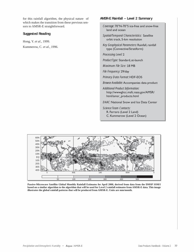
Data Products Handbook - Volume 2 77Precipitation and Atmospheric Humidity •
for this rainfall algorithm, the physical nature ofwhich makes the transition from these previous sen-sors to AMSR-E straightforward.
Suggested Reading
Hong, Y. et al., 1999.
Kummerow, C. et al., 1996.
Aqua / AMSR-E
60N
50N
40N
30N
20N
10N
EQ
10S
20S
30S
40S0 90E 180 90W 0
50 100 200 300 400 500
Passive-Microwave Satellite Global Monthly Rainfall Estimates for April 2000, derived from data from the DMSP SSM/Ibased on a similar algorithm to the algorithm that will be used for Level 2 rainfall estimates from AMSR-E data. This imageillustrates the global rainfall patterns that will be produced from AMSR-E. Units are mm/month.
AMSR-E Rainfall – Level 2 Summary
Coverage: 70°N-70°S ice-free and snow-freeland and ocean
Spatial/Temporal Characteristics: Satelliteorbit track, 5-km resolution
Key Geophysical Parameters: Rainfall, rainfalltype (Convective/Stratiform)
Processing Level: 2
Product Type: Standard, at-launch
Maximum File Size: 18 MB
File Frequency: 29/day
Primary Data Format: HDF-EOS
Browse Available: Accompanies data product
Additional Product Information:http://wwwghcc.msfc.nasa.gov/AMSR/html/amsr_products.html
DAAC: National Snow and Ice Data Center
Science Team Contacts:R. Ferraro (Level 2 Land)C. Kummerow (Level 2 Ocean)

78 Data Products Handbook - Volume 2 • Precipitation and Atmospheric HumidityAqua / AMSR-E
AMSR-E Rainfall – Level 3
Product Description
This product consists of mean monthly rainfallamounts over 5° × 5° cells. Retrievals over oceanare independent of the Level 2 algorithm. Monthlyaccumulations over land use the Level 2 land prod-uct as input. Over oceans, this approach sacrificessome of the accuracy of the instantaneous retrievalin order to minimize assumptions that might contami-nate a climate record of rainfall. The frequency ofoccurrence of rain intensities in different rate catego-ries over a specified area can be plotted as a histo-gram or as a smoothed curve that fits the histogram.This product is obtained by considering histogramsof 19-GHz, 21-GHz, and 19-21 GHz combinations.Monthly rainfall indices are computed by statisticallymatching the histograms with the model-calculatedprobability density functions (pdf). The main purposeof this product is to provide a robust baseline of sur-face-rainfall rates. There is no equivalent indepen-dent method for estimating rainfall over land, andthe Level 2 product is therefore used as input to thepdf scheme.
This Level 3 rainfall product uses the Level 2AAMSR-E brightness temperatures as well as theAMSR-E Level 2 rainfall product as input. The Level3 product uses the Level 2A brightness temperaturesto estimate rainfall independently over oceans andthe Level 2 rainfall product over land to computemonthly accumulations.
Research and Applications
This product is designed to advance understandingof the Earth’s global energy and water cycles by de-termining how rainfall and its variability influenceglobal circulation. A reliable measurement of rain-fall, particularly over the oceans, will provide thelong-term record needed to distinguish natural vari-ability from any anthropogenic changes.
Data Set Evolution
The AMSR-E instrument is very similar to the TRMMTMI and the DMSP SSM/I. The algorithm overoceans will be a slight modification of the algorithmfor the TMI standard product and the WMO GlobalPrecipitation Climatology Project (GPCP) algorithmapplied to SSM/I. Data are already available fromthese algorithms for the period since 1987.
Suggested Reading
Chang, A.T.C. et al., 1999.
Wilheit, T.T. et al., 1991.
AMSR-E Rainfall – Level 3 Summary
Coverage: 70ºN-70ºS
Spatial/Temporal Characteristics: 5º × 5º/monthly
Key Geophysical Parameters: Rainfall amountand statistics
Processing Level: 3
Product Type: Standard, at-launch
Maximum File Size: 0.016 MB
File Frequency: 1/month
Primary Data Format: HDF-EOS
Browse Available: Accompanies data product
Additional Product Information:http://wwwghcc.msfc.nasa.gov/AMSR/html/amsr_products.html
DAAC: National Snow and Ice Data Center
Science Team Contact:T. T. Wilheit

Data Products Handbook - Volume 2 79Precipitation and Atmospheric Humidity •
diosonde observation and the 25-km SSM/I footprint.Computer simulations show that the true rms accu-racy of the microwave water-vapor retrievals is about1 mm. The AMSR-E retrievals should be more accu-rate than those from SSM/I because AMSR-E has adual-polarization water-vapor channel whereasSSM/I only had vertical polarization. Also, theAMSR-E water-vapor signal will not saturate in thetropics because its water-vapor channel is at 23.8 GHzrather than at the center of the water-vapor absorp-tion line (22.235 GHz). (SSM/I operated at 22.235GHz and experienced partial saturation in the trop-ics.)
Suggested Reading
Alishouse, J.C. et al., 1990.
Chahine, M.T., 1992.
Chang A.T.C., and T.T. Wilheit, 1979.
Chang, H.D. et al., 1984.
Grody, N.C., 1976.
Liu, W.T. et al., 1992.
Ramanathan, V., 1988.
Staelin, D.H. et al., 1976.
Wentz, F.J., 1997.
Aqua / AMSR-E
AMSR-E Columnar Water Vapor
Product Description
The columnar water vapor derived from the AMSR-E microwave radiances is a measure of the total ver-tically integrated water vapor in the marine atmo-sphere. It is expressed in units of millimeters, whichrepresent the depth of the column of liquid water thatwould result if the vapor were to precipitate com-pletely. The spatial resolution of this product is 20km, and its expected rms accuracy at this resolutionis 1.0 mm. This product is available for clear andcloudy conditions and up-to-moderate rain rates. Theproduct will be produced for individual pixels acrossthe AMSR-E swath (Level 2) as well as an Earth-gridded product (0.25° in latitude and longitude) av-eraged daily, weekly, and monthly (Level 3).
Research and Applications
Column water vapor is a critical component couplingthe atmosphere and oceans, transporting energy inthe form of latent heat from the ocean surface to theatmosphere, where it is released through condensa-tion. Furthermore, water vapor is the Earth’s princi-pal greenhouse gas, trapping sufficient heat to main-tain the average surface temperature above freezing,and therefore is responsible for the habitability of theplanet. Within the context of global-change studies,the possibility of positive feedback between anthro-pogenic carbon dioxide and water vapor has becomea particularly active research area, largely due tomodel predictions of significant amplification ofgreenhouse heat trapping by concomitant rises in at-mospheric water vapor. Sensitive and accurate long-term measurements of spatial and temporal variabil-ity in this quantity also constitute, along withmeasurements of air and sea-surface temperature, avaluable geophysical data set for monitoring globalchange.
Data Set Evolution
The water-vapor retrieval algorithm is based on ex-perience gained from previous microwave radiom-eters, including SMMR, SSM/I, and TMI. In particu-lar, the SSM/I has demonstrated the ability ofmicrowave radiometers to measure water vapor toan accuracy of about 1 mm. For 35,000 SSM/I over-flights of radiosondes (1987-1991), the rms differ-ence between the SSM/I and radiosonde water vaporis 3.9 mm, with most of this difference being due tothe spatial-temporal mismatch between the point ra-

80 Data Products Handbook - Volume 2 • Precipitation and Atmospheric Humidity
MODIS Total Precipitable Water(MOD 05)
Product Description
The MODIS Precipitable Water product (MOD 05)consists of column water-vapor amounts. During thedaytime, a near-infrared algorithm is applied overclear land areas of the globe and above clouds overboth land and ocean. Over clear ocean areas, water-vapor estimates are provided over the extended glintarea. An infrared algorithm for deriving atmosphericprofiles is also applied both day and night for Level2.
The Level 2 data are generated at the 1-km spatialresolution of the MODIS instrument using the near-infrared algorithm during the day, and at 5 × 5 1-kmpixel resolution both day and night using the infra-red algorithm when at least nine FOVs are cloud free.The infrared-derived precipitable water vapor is gen-erated as one component of product MOD 07, andsimply added to product MOD 05 for convenience.
The solar retrieval algorithm relies on observationsof water-vapor attenuation of reflected solar radia-tion in the near-infrared MODIS channels so that theproduct is produced only over areas where there is areflective surface in the near IR.
Research and Applications
The near-infrared total-column precipitable water isvery sensitive to boundary-layer water vapor since itis derived from attenuation of reflected solar lightfrom the surface. This data product is essential tounderstanding the hydrological cycle, aerosol prop-erties, aerosol-cloud interactions, energy budget, andclimate. Of particular interest is the collection ofwater-vapor data above cirrus cloudiness, which hasimportant applications to climate studies. MODISwill also provide finer horizontal-scale atmosphericwater-vapor gradient estimates than are currentlyavailable from the Polar-orbiting Operational Envi-ronmental Satellites (POES).
Data Set Evolution
The solar-column water-vapor parameter is derivedfrom the attenuation by water vapor of near-IR solarradiation. Techniques employing ratios of water-va-por-absorbing channels 17, 18, and 19 with the at-mospheric window channels 2 and 5 are used. Theratios remove partially the effects of variation of sur-face reflectance with wavelength and result in theatmospheric water-vapor transmittances. The col-
AMSR-E Columnar Water Vapor Summary
Coverage: Global ocean surface, clear andcloudy skies and up-to-moderate rainfallrates
Spatial/Temporal Characteristics:Level 2: swath pixels at 20-km resolutionLevel 3: 0.25° latitude-longitude grid/daily,weekly, and monthly
Key Science Applications: Climate variability,air-sea interaction, radiation balance,hydrological cycle
Key Geophysical Parameters: Columnar watervapor
Processing Level: 2, 3
Product Type: Standard, post-launch
Maximum File Size: 10 MB
File Frequency: 29/day
Primary Data Format: HDF-EOS
Browse Available: Accompanies data product
Additional Product Information:http://wwwghcc.msfc.nasa.gov/AMSR/html/amsr_products.html
DAAC: National Snow and Ice Data Center
Science Team Contact:F. J. Wentz
(AMSR-E Columnar Water Vapor, continued)
Aqua / AMSR-E and MODIS

Data Products Handbook - Volume 2 81Precipitation and Atmospheric Humidity • Aqua / MODIS
umn-water-vapor amounts are derived from the trans-mittances based on theoretical radiative-transfer cal-culations and using look-up-table procedures. MO-DIS is the first space instrument to use near-IR bandstogether with the traditional IR bands to retrieve to-tal precipitable water. Experience in this retrieval isbased on an AVIRIS instrument aboard an ER-2 air-craft. Atmospheric water vapor should be determinedwith an accuracy of 5-10%.
The thermal column water-vapor parameter is de-rived by integrating the moisture profile through theatmospheric column. Other, split-window, methodsalso exist. This class of techniques uses the differ-ence in water-vapor absorption that exists betweenchannel 31 (11 µm) and channel 32 (12 µm).
Data validation will be conducted by comparingthese data with water-vapor measurements from theNational Weather Service (NWS) radiosonde net-work, from ground-based upward-looking microwaveradiometers, from a ground-based GPS network, andfrom a ground-based sunphotometer network. Qual-ity control will be performed in two dimensions. Thefirst will be comparisons of specific validation sitesacross as many different climatic and geographic re-gions as possible. The second will be a statisticalanalysis of the entire data set.
The related MODIS Cloud product ATBDs can befound in PDF format at http://eos.nasa.gov/atbd/modistables.html.
Suggested Reading
Gao, B.C., and A.F.H. Goetz, 1990.
Gao, B.C. et al., 1993a,b.
Green, R.O., and J.E. Conel, 1995.
Jedlovec, G.J., 1987.
Kaufman, Y.J., and B.C. Gao, 1992.
King, M.D. et al., 1992.
Kleepsies, T.J., and L.M. McMillan, 1984.
MODIS Total Precipitable Water Summary
Coverage: Global
Spatial/Temporal Characteristics: Varies withretrieval technique; 1 km near-infrareddaylight only, and 5 km infrared day andnight
Key Science Applications: Hydrological cycleclimatology, effect on aerosol and clouds,atmospheric correction, characterization ofthe atmosphere
Key Geophysical Parameters: Atmospheric totalcolumn water vapor
Processing Level: 2
Product Type: Standard, at-launch
Maximum File Size: 15 MB
File Frequency: 288/day
Primary Data Format: HDF-EOS
Browse Available:http://modis-atmos.gsfc.nasa.gov/MOD05_L2/sample.html
Additional Product Information:http://modis-atmos.gsfc.nasa.gov/MOD05_L2/index.html
Science Team Contacts:B.C. GaoY.J. KaufmanD. TanréW.P. Menzel
Sample Columnar Atmospheric Water Vapor from Terra MODIS data from the vicinity of Tibet and India on March 2, 2000, at UTC0525. These results are derived from data from channels located within and around the 0.94-µm water vapor band. The left panelshows an image processed from MODIS channels centered at 0.645 µm. The lower part of the scene covers portions of India and thenearby Indian Ocean. The upper part of the scene covers Nepal and part of the Tibetan Plateau. The middle panel shows the MODIScolumn water vapor. The right panel shows the corresponding image of surface elevations. It is seen from these images that columnwater vapor values vary significantly with surface elevation.
5.0
4.0
3.0
2.0
1.0
0.0
Meters6000
5000
4000
3000
2000
1000
0
Reflectance (0.645 µm) Water Vapor (cm) Elevation

82 Data Products Handbook - Volume 2 • Precipitation and Atmospheric Humidity
MODIS Atmospheric Profiles(MOD 07)
Product Description
The MODIS Atmospheric Profiles product (MOD 07)consists of several parameters: they are total-ozoneburden, atmospheric stability, temperature and mois-ture profiles, and atmospheric water vapor. All ofthese parameters are produced day and night for Level2 at 5 × 5 1-km pixel resolution when at least 9 FOVsare cloud free.
The MODIS total-ozone burden is an estimate ofthe total-column tropospheric and stratospheric ozonecontent. The MODIS atmospheric stability consistsof three daily Level 2 atmospheric stability indices.The Total Totals (TT), the Lifted Index (LI), and theK index (K) are each computed using the infraredtemperature- and moisture-profile data, also derivedas part of MOD 07. The MODIS temperature andmoisture profiles are produced at 20 vertical levelsfor temperature and 15 levels for moisture. A simul-taneous direct physical solution to the infrared radia-tive-transfer equation in a cloudless sky is used. TheMODIS atmospheric water-vapor product is an esti-mate of the total tropospheric column water vapormade from integrated MODIS infrared retrievals ofatmospheric moisture profiles in clear scenes.
Research and Applications
Total-column ozone estimates at MODIS resolutionare required by MODIS investigators developing at-mospheric correction algorithms. This informationis crucial for accurate land and ocean-surface-param-eter retrievals. Furthermore, strong correlations havebeen found to exist between the meridional gradientof total ozone and the wind velocity at tropopauselevels, providing the potential to predict the positionand intensity of jet streams. Total-column ozonemonitoring is also important due to the potential harmto the environment caused by anthropogenic deple-tion of ozone.
Atmospheric instability measurements are predic-tors of convective-cloud formation and precipitation.The MODIS instrument offers an opportunity to char-acterize gradients of atmospheric stability at highresolution and greater coverage. Radiosonde-derivedstability indices are limited by the coarse spacing ofthe point-source data, too large to pinpoint local re-gions of probable convection.
Atmospheric temperature and moisture soundingdata at high spatial resolution from MODIS and high-
spectral-resolution sounding data from AIRS will pro-vide a wealth of new information on atmosphericstructure in clear skies. The profiles will be used tocorrect for atmospheric effects for some of the MO-DIS products (e.g., sea-surface and land-surface tem-peratures, ocean aerosol properties, water-leaving ra-diances, and PAR) as well as to characterize theatmosphere for global greenhouse studies.
Total-column precipitable-water estimates at MO-DIS resolution are required by MODIS investigatorsdeveloping atmospheric-correction algorithms. Thisinformation is crucial for accurate land and oceansurface-parameter retrievals. MODIS will also pro-vide finer horizontal-scale atmospheric water-vaporgradient estimates than are currently available fromthe POES satellites.
Data Set Evolution
One of two ozone-retrieval methods developed us-ing the HIRS will be chosen as best suited for appli-cation with MODIS data. Both use a first-guess per-turbation method and radiances from MODIS channel30 (9.6 µm) to solve the radiative-transfer equation.The perturbations are with respect to some a prioriconditions that may be estimated from climatology,regression, or, more commonly, from an analysis orforecast provided by a numerical model. The MO-DIS cloud-mask product (MOD 35) will also be usedto screen for clouds.
Atmospheric-stability estimates will be derivedfrom the MODIS temperature and moisture retriev-als contained in this product. Layer temperature andmoisture values may be used to estimate the tem-perature lapse rate of the lower troposphere and thelow-level moisture concentration.
Temperature and moisture profile retrieval algo-rithms are adapted from the International TOVS Pro-cessing Package (ITPP), taking into account MODIS’lack of stratospheric channels and far higher hori-zontal resolution. The profile retrieval algorithm re-quires calibrated, navigated, and coregistered 1-kmFOV radiances from MODIS channels 20, 22-25, 27-29, and 30-36. The MODIS cloud mask (MOD 35)is used for cloud screening. The algorithm also re-quires NCEP model analyses of temperature andmoisture profiles as a first guess and an NCEP analy-sis of surface temperature and pressure.
Several algorithms for determining atmosphericwater vapor, or precipitable water, exist. It is mostdirectly achieved by integrating the moisture profilethrough the atmospheric column. Other, split-win-dow, methods also exist. This class of techniques uses
Aqua / MODIS

Data Products Handbook - Volume 2 83Precipitation and Atmospheric Humidity • Aqua / MODIS
the difference in water-vapor absorption that existsbetween channel 31 (11 µm) and channel 32 (12 µm).
Data validation will be conducted by comparingresults to in situ radiosonde measurements, NOAAHIRS operational retrievals, GOES sounder opera-tional retrievals, NCEP analyses, and retrievals fromthe AIRS/AMSU-A/HSB instrument package on theAqua platform. A field campaign using a profiler net-work in the central U.S. and an aircraft equipped withthe MODIS Airborne Simulator (MAS) will be initi-ated in the first year after launch. Quality control willconsist of manual and automatic inspections, withregional and global mean temperatures at 300, 500,and 700 hPa monitored weekly, along with 700 hPadew-point temperatures. For total ozone, data vali-dation will consist of comparing the TOMS retriev-als, as well as operational NOAA ozone estimatesfrom HIRS, to the MODIS retrievals.
Suggested Reading
Hayden, C.M., 1988.
Houghton, J.T. et al., 1984.
Jedlovec, G.J., 1987.
Kleepsies, T.J., and L.M. McMillan, 1984.
Ma, X.L. et al., 1984.
Prabhakara, C. et al., 1970.
Shapiro, M.A. et al., 1982.
Smith, W.L., and F.X. Zhou, 1982.
Smith, W.L. et al., 1985.
Sullivan, J. et al., 1993.
MODIS Atmospheric Profiles Summary
Coverage: Global, clear-sky only
Spatial/Temporal Characteristics: 5 km
Key Science Applications:•Ozone: atmospheric correction, predic-tion of cyclogenesis, anthropogenicozone depletion
•Atmospheric stability: atmosphericcorrection, prediction of convectivecloudiness and precipitation, character-ization of the atmosphere
•Soundings: atmospheric correctionalgorithm development and use, charac-terization of the atmosphere
•Total-column water vapor: atmospheric-correction algorithm development anduse, characterization of the atmosphere
Key Geophysical Parameters: Total-columnozone, atmospheric stability (Total Totals,Lifted Index, and K index), atmosphericprofiles of temperature and moisture,atmospheric total-column water vapor
Processing Level: 2
Product Type: Standard, at-launch
Maximum File Size: 28 MB
File Frequency: 288/day
Primary Data Format: HDF-EOS
Browse Available:http://modis-atmos.gsfc.nasa.gov/MOD07_L2/sample.html
Additional Product Information:http://modis-atmos.gsfc.nasa.gov/MOD07_L2/index.html
Science Team Contact:W.P. Menzel

84 Data Products Handbook - Volume 2 • Precipitation and Atmospheric Humidity
Level 2 MODIS Atmospheric Temperature (K) at 500 hPa (upper panel) and Level 2 MODIS Total Column Precipi-table Water Vapor (cm) (lower panel), both derived from data taken over the Himalayas and Northern India at 5:25UTC on April 19, 2000, from the MODIS instrument on Terra.
Atmospheric Temperature at 500 hPa
Total Column Precipitable Water Vapor
Aqua / MODIS
(MODIS Atmospheric Profiles, continued)
Data Products Handbook - Volume 2 85Precipitation and Atmospheric Humidity • Jason-1 / JMR
JMR Columnar Water VaporContent
Product Description
This Level 2 product provides the measurement ofthe total atmospheric columnar water vapor content(in g/cm2) made by the Jason-1 Microwave Radiom-eter (JMR). The measurement is repeated every 9.9days along a set of fixed ground tracks. The satellitemakes 127 revolutions of the Earth every 9.9 days.The coverage of the measurement is limited from 66°S to 66° N due to the 66° inclination of the satellite’sorbit plane. The longitudinal distance between theground tracks is [315.cos(latitude)] km, i.e., 315 kmat the equator, 223 km at 45°, and 128 km at 66°.This product is used to generate gridded Level 3 prod-ucts by various Jason-1 Science Working Team mem-bers. Two kinds of product are available: The InterimGeophysical Data Record (IGDR) is available 3 daysafter the data collection, while the GDR, based on amore precisely determined orbit, is available 30 daysafter the data collection.
Research and Applications
Water vapor is the most important greenhouse gas inthe atmosphere. It plays a large role in keeping theEarth at a temperature suitable for intelligent life.Furthermore, information on the content of watervapor and its variability is important for the study ofclimate in other ways as well. For example, the wa-ter vapor measurement made by the TOPEX Micro-wave Radiometer was used to study the relationshipbetween the 1997-98 El Niño and the variability oftotal water vapor content of the Earth.
Data Set Evolution
The JMR measures the brightness temperature of thesea surface at three frequencies: 18.7, 23.8, and 34GHz. These measurements are used to compute therange delay of radar altimeter signals due to the wa-ter vapor in the atmosphere as well as the total co-lumnar water vapor content. The antenna tempera-tures measured by JMR are first converted intobrightness temperatures of the sea surface at the threefrequencies. The brightness temperatures are thenused to compute the total water vapor content alongthe path of the JMR line of sight. The primary heri-tage for the JMR water vapor product is the corre-sponding product derived from the data of the
TOPEX/Poseidon Microwave Radiometer, launchedin 1992.
Suggested Reading
Haines, B.J., and Y.E. Bar-Sever, 1998.
Nerem, R.S. et al., 1999.
Ruf, C.S. et al., 1994.
JMR Columnar Water Vapor ContentSummary
Coverage: Ocean areas from 66° S to 66° N.
Spatial/Temporal Characteristics: 6.2-kmresolution along-track every 9.9 days;[315·cos(latitude)] km longitudinal trackspacing
Key Science Applications: Greenhouse gasmonitoring, climate change
Key Geophysical Parameters: Atmosphericcolumnar water vapor content
Processing Level: 2
Product Type: Standard, at-launch
Maximum File Size: 1.5 MB
File Frequency: 25/day
Primary Data Format: Binary
Browse Available: Yes
Additional Product Information:http://www-aviso.cnes.fr
DAAC: Jet Propulsion Laboratory
Science Team Contacts:L.-L. FuY. Ménard

86 Data Products Handbook - Volume 2 • Precipitation and Atmospheric Humidity
SAGE III Water Vapor Products(SAGE III 03)
Product Description
The SAGE III Water Vapor Products (SAGE III 03at Level 2) consist of H2O concentration (number den-sity in units of molecules/cm3) and volume mixingratio (ppmv) at each measurement location with avertical resolution of 0.5 km. The water-vapor prod-ucts are retrieved from the solar-occultation measure-ments of slant-path absorption using 29 contiguoussubchannels between 933.19 nm and 960.12 nm,spaced at approximately 1 nm with a resolution ofabout 1.4 nm.
Since temperature profiles will also be measuredby SAGE III, utilizing the oxygen A-band absorp-tion spectra in the wavelength region 759-771 nm,relative humidities can be derived accordingly, us-ing the SAGE III-retrieved water-vapor profiles andtemperature profiles.
Research and Applications
SAGE III water-vapor profiles will provide comple-mentary measurements to those of other EOS instru-ments. With its vertical resolution of 0.5 km, SAGEIII water-vapor products are necessary for unravel-ing the issues associated with troposphere-strato-sphere water-vapor exchange. Since the occultationmeasurements are relatively immune to drift in in-strument performance, SAGE III-retrieved water-vapor profiles are invaluable for helping to validateobservations from the other EOS-system instruments.Furthermore, given the long-term reliability and self-calibration capabilities of the SAGE instruments,SAGE III may be in a position to evaluate water-vapor trends in the upper troposphere and lowerstratosphere during a time period when considerablewarming due to increased emissions of human-de-rived greenhouse gases may occur.
SAGE III Water Vapor Products Summary
Coverage: 30 solar events per day, 15northern high latitude, 15 southern highlatitude
Spatial/Temporal Characteristics: 0.5 kmvertical resolution
Key Science Applications: Greenhouse effect,global warming, validation of climatemodels, convective cloud studies,weather-forecast initialization, tropo-spheric chemistry, stratospheric chemis-try
Key Geophysical Parameters: Water-vaporconcentration, water-vapor mixing ratios,relative humidities, total-column watervapor, moisture content
Processing Level: 2
Product Type: Standard, at-launch
Maximum File Size: 0.05 MB
File Frequency: 196/week
Primary Data Format: HDF-EOS, Big EndianIEEE Binary
Browse Available: Yes
Additional Product Information:http://eosweb.larc.nasa.gov/PRODOCS/sage3/table_sage3.html
DAAC: NASA Langley Research Center
Science Team Contact:E.-W. Chiou
Meteor 3M / SAGE III

87
Cloud and AerosolPropertiesandRadiative Energy Fluxes
Aqua• AIRS
• AMSR-E• AMSU-A
• CERES• HSB
• MODIS
Meteor 3M• SAGE III
QuikTOMS• TOMS

88 Data Products Handbook - Volume 2 Overview • Cloud and Aerosol Properties and Radiative Energy Fluxes
Cloud and Aerosol Properties andRadiative Energy Fluxes – AnOverview
Relationship to Global Change Issues
Clouds and aerosols play a significant role in modi-fying the flow of energy to and from the Earth’s sur-face. Hence, measuring and understanding clouds andaerosols are among the keys to predicting climatechange and to testing global climate models. The tech-nology for measuring radiative fluxes, cloud proper-ties, and aerosol properties from space is now suffi-ciently advanced that these measurements can be usedto improve significantly our ability to address suchcritical global change issues as whether clouds act asa positive or negative feedback mechanism as cli-mate changes and whether aerosols will offset someof the expected warming from increasing greenhousegases.
In many cases, cloud and/or aerosol studies usingthe data from the missions highlighted in this vol-ume will benefit from instruments on other satellitemissions as well. In particular, versions of the CERESinstrument will be operating on the TRMM, Terra,and Aqua platforms and will function synergisticallyin conjunction with VIRS and TMI (on TRMM), MO-DIS and MISR (on Terra), and MODIS and AMSR-E (on Aqua). Similarly, the MODIS instruments onTerra and Aqua will complement each other by pro-viding morning and afternoon measurements, respec-tively.
Clouds: A first step in examining clouds from spaceis to determine their distribution through the atmo-sphere, i.e, where they are and what their dimensionsare. Once clouds are identified and mapped, cloudproperties such as effective particle size, thermody-namic phase (water, ice), cloud-top properties, andoptical thickness (all of which help determine howmuch radiation passes through them) may be mea-sured. The MODIS, AIRS/AMSU-A/HSB, andAMSR-E instruments on the EOS Aqua platform, theSAGE III instrument on the Meteor 3M platform,the MODIS, MISR, and ASTER instruments on theEOS Terra platform (see Volume 1), and the VIRSand TMI instruments on TRMM (see Volume 1) willprovide these key cloud measurements. The daily ob-servations from these instruments also provide thesampling needed to drive and verify climate models.In the longer term, advances are expected in the ver-tical distribution of clouds using the active lidar andcloud radar data from the PICASSO-CENA andCloudSat missions flying in formation with Aquastarting in 2003.
Aerosols: Aerosols are suspended particles in the at-mosphere such as dust, sulfate, smoke, and many oth-ers. Their measurement is an important element indescribing energy transmission through the atmo-sphere. Uncertainties regarding aerosols result in theirbeing a significant source of uncertainty in climatemodeling. They affect cloud microphysics by actingas condensation nuclei, thereby affecting cloud ra-diative properties. They also interact directly withsolar radiation, thus affecting the radiative balance;and the geographic locations of anthropogenic aero-sols are also important considerations in their impacton climate. In addition, stratospheric aerosols play arole in the ozone depletion issue through heteroge-neous chemistry. Aerosol products described here,derived from MODIS on Aqua, and those from MO-DIS and MISR on Terra, will provide new informa-tion on aerosol formation, distribution, and sinks overboth the land and ocean. Aerosol data from SAGE IIIon Meteor 3M will provide altitude profiles of aero-sols and polar stratospheric cloud information fromthe upper troposphere through the stratosphere in thehigh-latitude regions. In the longer term, advancesare expected in determining the vertical distributionof aerosols in the troposphere using the active lidaron the PICASSO-CENA mission.
Radiation: The flow of radiation from the Sun to theEarth and its absorption, reflection, and emissionwithin the Earth system determine the energy bal-ance of the Earth and hence have a significant effecton the nature of life on Earth as well. The informa-tion from products describing optical and physicalproperties of clouds and aerosols is combined withbroadband radiation measurements from CERES andAIRS to provide estimates of solar and infrared ra-diative fluxes, which in turn determine the heatingand cooling of the Earth and the atmosphere. Theradiation estimates needed to do this are both short-wave and longwave fluxes at the surface and at thetop of the atmosphere, both downwelling and up-welling, so that the net flow can be determined. Also,fluxes must be distinguished between cloudy- andclear-sky regions, and the fluxes over a series of el-evation intervals are needed to test atmospheric mod-els. Improved knowledge of the vertical distributionof radiative fluxes will be obtained by the additionof PICASSO-CENA and CloudSat data, with theseplatforms flying in formation with Aqua.
Product Overview
CERES will continue the fifteen-year record of ra-diation-budget information produced by the ERBE

Data Products Handbook - Volume 2 89Cloud and Aerosol Properties and Radiative Energy Fluxes • Overview
program. As with Terra, starting 6 months after thelaunch of Aqua (following instrument and analysisvalidation), the CERES science team will begin pro-duction of ERBE-like data products. These top-of-the-atmosphere (TOA) fluxes will use the ERBEanalysis algorithms to allow consistent comparisonsto historical ERBE data. Furthermore, the data fromthe first 24 months after the Terra and Aqua launcheswill be used to develop a new set of CERES angulardistribution models (ADMs). These ADMs are usedto convert broadband CERES radiances, i.e., radia-tive energy at a single viewing direction, into esti-mates of broadband hemispheric fluxes. The CERESrotating-azimuth-plane scan mode will be used alongwith the cloud properties derived using VIRS andMODIS data to derive new and much more accurateADMs. Beginning 30 months after launch, these moreaccurate CERES estimated TOA fluxes will be pro-duced in addition to the ERBE-like products. Finally,starting 36 months after launch, CERES will routinelyprovide estimates of radiative fluxes at the surfaceand at a selected number of levels within the atmo-sphere. The number of atmospheric levels will de-pend on the accuracies determined during post-launchvalidation.
All the CERES products except the ERBE-likeproducts are classified as “post-launch” for the rea-sons discussed above. The AMSR-E product in thischapter is also post-launch, while the AIRS/AMSU-A/HSB, MODIS, SAGE III, and TOMS products are“at-launch.”
The cloud products fall into two classes: 1) clouddetection and delineation, and 2) cloud properties.Cloud detection and delineation produces masks in-dicating where clouds exist and information on lay-ering and overlap to give a geometric picture of glo-bal cloud coverage. Cloud properties include opticalthickness, temperature, liquid-water content, ice-water content, particle radius, cloud-top altitude, andphase, all of which relate to the radiative transmis-sion, reflection, and emission of the clouds.
The CERES cloud-detection process uses obser-vations from VIRS on TRMM and MODIS on Terraand Aqua to produce a global binary mask indicatingthe presence or absence of a cloud in each imagerpixel mapped to the CERES fields of view. TheMODIS cloud mask (MOD 35) is a global productthat provides a probability that a view of the Earth isobstructed by clouds and an indication of whethercloud shadow is detected. It also provides informa-tion on land/sea presence and day/night conditions.
MODIS cloud-property parameters include par-ticle size and phase, optical thickness, cloud-topheight, emissivity and temperature, and cloud frac-tion in a region, all of which support specific MO-
DIS science tasks that complement the radiation stud-ies and products from other instruments. CEREScloud properties include cloud-layer mapping, cloud-top and cloud-base pressure, infrared emissivity, liq-uid-water path, particle radius, and cloud overlap, allderived from MODIS or VIRS data and remappedonto the broadband CERES fields of view for stud-ies of the Earth’s radiative-energy distribution. AIRS/AMSU-A/HSB cloud properties include cloud-toppressure, temperature, and cloud spectral properties,while AMSR-E data will be used to derive columnarcloud water.
Aerosol properties are provided by SAGE III onMeteor 3M, TOMS on QuikTOMS, and MODIS(MOD 04) on Aqua. Aerosols must be accounted forduring the retrieval of surface and atmospheric pa-rameters for maximum accuracy. The MODIS aero-sol products include aerosol optical thickness, aero-sol size distribution, and aerosol sources and sinks;SAGE III products include multi-spectral extinctionprofiles of aerosols with high vertical resolution fromthe upper troposphere through the stratosphere; andTOMS products include an aerosol index derivedfrom backscattered ultraviolet radiances. These vari-ous aerosol products will aid both in understandingthe role of aerosols in the climate system and in im-proving corrections for aerosol effects in the retrievalof surface parameters.
Radiant energy flux products from CERES includethe radiative fluxes downward and upward at the topof the atmosphere, at the Earth’s surface, and at se-lected intermediate altitudes, as well as the net flux,which is used to determine the radiation budget. Thisbudget in turn determines the overall heating andcooling of the atmosphere and the Earth’s surface andhence has a central role in climate changes. TheCERES radiation algorithms use the cloud and aero-sol products in the calculations for determining howmuch solar radiation is transmitted, reflected, and ab-sorbed in the cloud/atmosphere/Earth-surface system.They are thus critical in the monitoring of global cli-mate.
Product Interdependency and Continuitywith Heritage Data
There is significant interdependency both amongstthe products described in this chapter and betweenthese products and data from other sources. In manycases, output data from one instrument become in-put ancillary data for another, as in the case of MO-DIS and/or TRMM data being used in the calcula-tion of CERES cloud products. Further, the clouddistributions will be used in cloud masks for surfaceproducts.

90 Data Products Handbook - Volume 2 • Cloud and Aerosol Properties and Radiative Energy Fluxes
The AIRS/AMSU-A/HSB cloud products build onthe heritage of HIRS/MSU, the AMSR-E productson the heritage of SMMR, SSM/I, and TMI, theCERES products on the heritage of ERBE, the MO-DIS products on the heritage of AVHRR, the SAGEIII products on the heritage of SAM II, SAGE I, andSAGE II, and the QuikTOMS products on the heri-tage of earlier TOMS instruments. In the case ofCERES, several data products use ERBE algorithmsto ensure continuity with the extensively analyzedERBE data set. Similarly, the SAGE III data will beused to derive aerosol products with an algorithmsimilar to the SAGE II algorithm, to ensure continu-ity of the SAGE aerosol products. The continuationof existent data records will assist the determinationof long-term trends and the analysis of the role ofclouds, aerosols, and radiative energy fluxes in glo-bal climate and climate change.
Suggested Reading
Barkstrom, B.R., 1984.
Coakley, J. et al., 1983.
Di Girolamo, L., and R. Davis, 1994.
Diner, D.J. et al., 1991.
Dubovik, O. et al., 2000.
Goodman, A.H., and A. Henderson-Sellers, 1988.
Hansen, J. et al., 1993.
Holben, B.N. et al., 1992.
Kaufman, Y.J., and C. Sendra, 1988.
Kaufman, Y.J. et al., 1997a,b.
King, M.D., 1987.
King, M.D. et al., 1992.
King, M.D. et al., 1999.
Ramanathan, V., 1986.
Ramanathan, V., 1987.
Ramanathan, V. et al., 1989.
Randall, D.A. et al., 1989.
Remer, L.A., and Y.J. Kaufman, 1998.
Remer, L.A. et al., 1997.
Remer, L.A. et al., 1998.
Sohn, B.-J., and F.R. Robertson, 1993.
Solomon, S. et al., 1997.
Tanré, D. et al., 1996.
Wang, M., and H.R. Gordon, 1994.
Wielicki, B.A. et al., 1995.
Wielicki, B.A. et al., 1996.
Wielicki, B.A. et al., 1998.
Overview • Cloud and Aerosol Properties and Radiative Energy Fluxes
(Cloud and Aerosol Properties and Radiative Energy Fluxes –An Overview, continued)

Data Products Handbook - Volume 2 91Cloud and Aerosol Properties and Radiative Energy Fluxes •
AIRS/AMSU-A/HSB CloudProduct (AIR 04)
Product Description
The AIRS Cloud Product (AIR 04) employs micro-wave, infrared, and visible observations to determinethe physical and radiative cloud properties within anAMSU-A field of view (FOV).
The product consists of cloud-top pressure for up-to-two cloud layers within an AMSU-A FOV, effec-tive fractional cloud-cover values for each AIRS foot-print and cloud type, and the ratio of the spectral emis-sivity at a number of frequencies to that at 11 µm forthe top cloud layer. The effective fractional cloudcover is the product of the geometrical fractionalcloud cover and the 11-µm cloud emissivity.
Cloud parameters are retrieved for each AIRS foot-print, regardless of whether a microwave/infrared(MW/IR) temperature profile can be successfully re-trieved.
The product is generated daily (day and night) atAMSU-A FOV resolution, with some information atAIRS FOV resolution.
A visible cloud product is available at AIRS foot-print resolution during daylight. The product consistsof cloud amount (distinguishing between high andlow clouds) and variability index within the AMSU-Afootprint.
Research and Applications
Cloud parameters are important for studying inter-annual variability, and cloudiness is the principalmodulating factor on shortwave- and longwave- ra-diation fluxes. Because of their high spatial and tem-poral variability, the effect of clouds is important overa wide range of spatial and temporal scales. Mostcurrent estimates of cloud amount (fractional cloudcover) are based on observations made at the ground.The accuracy of these values is doubtful except forzero or 100% cloudiness. Several definitions ofcloudiness from space have been proposed. The defi-nition considered appropriate for sounders such asAIRS emphasizes that clouds are the forcing param-eters that make the observed infrared radiance differfrom clear-column radiance.
The AIRS effective fractional cloud cover derivedfrom the MW/IR retrieval is effective for longwave-flux calculations only and involves the cloud emis-sivity. Shortwave fluxes require effective cloud frac-tions utilizing the cloud albedo as well as the geo-metric cloud fraction.
Data Set Evolution
Radiances are cloud cleared to remove the effects ofclouds on the radiance, enabling geophysical param-eters to be determined for the clear portion of thescene. Assuming these parameters are valid over theentire scene, a set of cloud parameters is found which,when substituted in the radiative-transfer equations,best matches the observations for a number of chan-nels used to determine cloud properties. The geo-physical parameters used to determine the cloud pa-rameters are from the AIRS solution for the AMSU-A footprint, whether it is a combined MW/IR solu-tion in the case of accepted retrievals, or a primarilyMW solution in the case of rejected MW/IR profiles.
Visible observations are made at 2-km resolutionduring day portions of the orbits to determine a vis-ible cloud amount (distinguishing between high andlow clouds) and variability index within the AMSU-Afootprint. Visible observations made during the nightportions of the orbits are expected to consist only ofnoise, except where bright moonlight or man-madesources are present. Visible information is combinedto achieve AIRS IR spatial resolution.
Data validation will be accomplished through com-parison of the retrieved cloud parameters with cor-relative data sets from satellite imagers (AVHRR andits derivatives).
Suggested Reading
Aumann, H.H., and C. Miller, 1995.
Aumann, H.H. et al., 1999.
Chahine, M.T., 1977.
Chahine, M.T., 1982.
Chahine, M.T. et al., 1977.
Chahine, M.T. et al., 1997a,b,c.
Hofstader, M. et al., 1999.
Lambrigsten, B., 1996.
Susskind, J. et al., 1997.
Susskind, J. et al., 1998.
Aqua / AIRS/AMSU-A/HSB

92 Data Products Handbook - Volume 2 • Cloud and Aerosol Properties and Radiative Energy FluxesAqua / AIRS/AMSU-A/HSB
AIRS/AMSU-A/HSB Cloud Product Summary
Coverage: Global
Spatial/Temporal Characteristics: Resolution ofAMSU-A FOV (40.6 km at nadir); someparameters at AIRS FOV (13.5 km atnadir)/once or twice daily (varies withparameter)
Key Science Applications: Cloud parameteriza-tion, climate modeling, and monitoring;AIRS cloud-cleared radiances
Key Geophysical Parameters:• Fraction of FOV obscured by clouds and
number of resolved cloud formations• Cloud-top pressure, temperature, and
cloud spectral properties
Processing Level: 2
Product Type: Standard, at-launch (spectralemissivity is a research product)
Maximum File Size: 5 MB
File Frequency: 240/day
Primary Data Format: HDF-EOS
Browse Available: Yes
Additional Product Information:http://www-airs.jpl.nasa.gov/
DAAC: NASA Goddard Space Flight Center
Science Team Contacts:M.T. ChahineJ. Susskind
AIRS/AMSU-A/HSB Flux Product(AIR 10)
Product Description
The AIRS Flux Product is included in the Level 2retrieval data granules and is geolocated to an AMSU-A footprint.
AIRS radiative fluxes consist of clear-column ra-diances, total Outgoing Longwave Radiation (OLR),net surface longwave flux, and net surface shortwaveflux.
Clear-column radiances represent the radianceswhich would have gone to space at the angle of ob-servation if no clouds were present in the field ofview, and they are the radiances used to compute thefinal AIRS products. Clear-column radiances are pro-duced for each AMSU-A footprint in which a suc-cessful combined MW/IR retrieval can be produced.This occurs in most cases of up to 80% cloudiness inthe AMSU-A footprint and is expected roughly twothirds of the time.
Clear-column radiances at different zenith anglesshould not be averaged together to produce time-mean values because of their substantial zenith-angledependence.
OLR is a function of surface and atmospheric con-ditions, particularly cloud-top pressure and cloudamount. OLR will be produced for every AIRS foot-print. OLR is important for studying interannual vari-ability and has been used as a proxy for precipita-tion.
When compared to other measures of OLR, suchas those from CERES, OLR from AIRS also servesas a validation for the detailed AIRS surface and at-mospheric products. Net surface longwave flux is thedifference between the longwave flux leaving thesurface, which depends only on surface parameters,and longwave flux striking the surface, which de-pends on atmospheric parameters, including cloud-base pressure. This is not a retrieved parameter. Con-sequently, net surface longwave flux is more difficultto compute than OLR and is a research product. Onevalue will be produced for each AMSU-A footprint.
Net shortwave flux is the difference between theshortwave flux reaching the surface and that reflectedby the surface. The downwelling shortwave flux is afunction of the sun irradiance and the atmosphericproperties, mostly those of clouds (cloud cover andcloud optical depth). The upwelling shortwave fluxdepends on the downwelling flux and the surface al-bedo.
(AIRS/AMSU-A/HSB Cloud Product, continued)

Data Products Handbook - Volume 2 93Cloud and Aerosol Properties and Radiative Energy Fluxes •
Radiances in selected AIRS cloud-clearing chan-nels, together with all the microwave radiances, areused to determine the coefficients for each AMSU-Afootprint. Error estimates are computed theoreticallyfor each channel for each profile. Surface tempera-ture and emissivity variations within the AMSU-Afootprint will contribute to the error in the clear-col-umn radiances.
The procedure to compute OLR and downward fluxis analogous to the procedure used with HIRS2/MSUsounding data. Radiative-transfer calculations aredone separately for a number of spectral bands as afunction of the retrieved surface-skin temperature,band surface emissivity, temperature-water-vapor-ozone profile, and cloud parameters including bandcloud spectral emissivity. The calculation in eachband is done at a band effective zenith angle, differ-ent for upwelling and downwelling flux, and multi-plied by π to give total band flux. These are addedtogether to give the total OLR or downwelling long-wave flux.
The procedure to compute the downwelling andupwelling shortwave flux employs a radiative-trans-fer model that uses the broad AIRS VIS/IR channel 4,surface albedo, aerosol optical depth, and integratedwater vapor as input. The surface albedo is computedfrom AIRS Channel 4 clear-sky radiances using thesame radiative-transfer model. Clear-sky detectionis achieved using a combination of AIRS Channel 1and, for regions covered by land surfaces, normal-ized difference vegetation index (NDVI) computedby differencing AIRS Channels 2 and 3.
Data validation will be accomplished throughchecking the internal consistency of the Level 2 re-trieval and vicarious validation of AIRS and near-IRradiances against in situ measurements at DoE ARM/CART sites, Baseline Upper Air Network (BUAN)sites, and dedicated MODIS and ASTER validationsites.
Suggested Reading
Aumann, H.H. et al., 1999.
Chahine, M.T. et al., 1977.
Gautier, C., and M. Landsfeld, 1997.
Hofstadter, M. et al., 1999.
Lambrigsten, B., 1996.
Mehta, A., and J. Susskind, 1999.
Research and Applications
The study of the global hydrologic cycle and its cou-pling to the energy cycle is key to understanding themajor driving forces of the Earth’s climate system.AIRS will measure the major components of thesedriving forces, including the thermal structure of thesurface and atmosphere, amount and height of clouds,outgoing longwave infrared radiation, and distribu-tion of atmospheric water vapor.
If the net radiative energy flux at the top of theatmosphere (TOA) is combined with the net radia-tive energy flux at the Earth’s surface, the net atmo-spheric radiative cooling is obtained. The atmosphericradiative cooling is the net effect of the infrared emis-sion by the atmosphere, the absorption by the atmo-sphere of infrared radiation emitted by the Earth’ssurface, and the absorption by the atmosphere of so-lar radiation.
AIRS/AMSU-A/HSB will measure the spectralchanges in the longwave radiation going to space.Knowledge of the changes is needed to monitor theeffects of trace gases on global warming.
AIRS super-window channels will be able to ob-serve the surface with minimum spectral contamina-tion by the atmosphere. In addition, AIRS narrowspectral channels in the short-wavelength infrared re-gion will observe the atmospheric layers above theEarth’s surface with the highest vertical resolutionpossible with passive remote sensing. The observa-tions will enable investigations of the fluxes of en-ergy and water vapor between the atmosphere andthe surface, as well as studies of their effect on cli-mate.
Data Set Evolution
The AIRS Flux product is derived by integrating theobserved radiances in the infrared and near infrared.
Determination of the AIRS clear-column radiancesis the most important step in the AIRS retrieval pro-cess. The methodology implicitly assumes that geo-physical parameters in all nine AIRS footprints withinan AMSU-A footprint are otherwise homogeneousexcept for varying amounts of up to eight differenttypes of cloud formations. With this assumption, theclear-column radiances for all channels are given aslinear combinations of the observed radiances in thosechannels in the nine fields of view, with an unknownset of channel-independent coefficients, one for eachcloud formation.
Aqua / AIRS/AMSU-A/HSB

94 Data Products Handbook - Volume 2 • Cloud and Aerosol Properties and Radiative Energy Fluxes
AIRS/AMSU-A/HSB Flux Product Summary
Coverage: Global
Spatial/Temporal Characteristics: AMSU-AFOV resolution (40.6 km at nadir)/twicedaily
Key Science Applications: Radiation budget,climate modeling
Key Geophysical Parameters:• Clear-column radiance• TOA outgoing longwave spectral
radiative flux• Spectral features in longwave fluxes, both
land and ocean• Net surface longwave fluxes, both land
and ocean• Net surface and TOA outgoing short-
wave fluxes, both land and ocean• Surface albedo
Processing Level: 2
Product Type: Research, at-launch
Maximum File Size: 5 MB
File Frequency: 240/day
Primary Data Format: HDF-EOS
Browse Available: Yes
Additional Product Information:http://www-airs.jpl.nasa.gov/
DAAC: NASA Goddard Space Flight Center
Science Team Contacts:J. SusskindC. Gautier
Aqua / AIRS/AMSU-A/HSB and AMSR-E
(AIRS/AMSU-A/HSB Flux Product, continued) AMSR-E Columnar Cloud Water
Product Description
The columnar cloud water (L) derived from theAMSR-E microwave radiances is a measure of thetotal vertically integrated liquid cloud water in themarine atmosphere. It is expressed in units of milli-meters, which represent the depth of the column ofliquid water that would result if the cloud were toprecipitate completely. The spatial resolution of thisproduct is 12 km, and its expected rms accuracy atthis resolution is 0.02 mm. The product only includesthe liquid-water contribution due to cloud droplets,and does not include the larger raindrops. Cloud drop-lets are typically smaller than 100 µm, whereas rain-drops can reach sizes up to several millimeters. Atmicrowave frequencies, the radiative characteristicsof cloud droplets and raindrops are quite different.Hence when rain is present, the accuracy of the cloudproduct degrades due to the difficulty in separatingthe cloud water from the rain water. The product willbe produced for individual pixels across the AMSR-Eswath (Level 2) as well as an Earth-gridded product(0.25° in latitude and longitude) averaged daily,weekly, and monthly (Level 3).
Research and Applications
Clouds remain one of the most poorly understoodconstituents of the climate system, primarily becauseof their complex morphology and highly variableradiative effects. They have significant effects on theplanetary radiation balance through both their highalbedo in the visible and the direct absorption andre-emission of outgoing longwave radiation. Cloudscontribute to both positive greenhouse feedback fromincreased solar absorption and heat trapping and nega-tive feedback from increases in albedo and radiativecooling. Formation of clouds is directly related tothe conversion of latent heat to sensible heat, and isstrongly correlated with the distribution of atmo-spheric heating. Additionally, advection of cloudwater is critical in the redistribution of water throughprecipitation, forming a major link in the global hy-drological cycle, which is a major driving force inthe Earth’s climate. Due to the difficulties involvedin treating their manifold effects accurately, cloudsare generally regarded as the weak link in most cur-rent state-of-the-art models of climate, making im-provements in the observational cloud data sets ofparticular importance.

Data Products Handbook - Volume 2 95Cloud and Aerosol Properties and Radiative Energy Fluxes •
Data Set Evolution
The cloud-water retrieval algorithm is based on ex-perience gained from previous microwave radiom-eters, including SMMR, SSM/I, and TMI. In particu-lar, the SSM/I has demonstrated the ability ofmicrowave radiometers to measure the cloud con-tent over the world’s oceans. Unfortunately, there isno reliable “ground truth” with which to validate thecloud-water algorithm. Hence, we rely on computersimulations and statistical analyses to assess the per-formance of the algorithm. The AMSR-E L retriev-als should be more accurate than SSM/I retrievalsbecause AMSR-E has two additional sets of dual-polarization channels at 6.9 and 10.7 GHz, which helpseparate the cloud signal from the wind signal andremove crosstalk due to varying sea-surface tempera-ture.
Suggested Reading
Grody, N.C., 1976.
Liu, G., and J. Curry, 1993.
Ramanathan, V. et al., 1989.
Staelin, D.H. et al., 1976.
Trenberth, K.E., 1998.
Webster, P.J., 1994.
Weng, F., and N.C. Grody, 1994.
Wentz, F.J., 1997.
Wentz, F.J., and R.W. Spencer, 1998.
AMSR-E Columnar Cloud Water Summary
Coverage: Global ocean surface, clear andcloudy skies and light rainfall
Spatial/Temporal Characteristics:Level 2: swath pixels at 12-km resolutionLevel 3: 0.25° latitude-longitude grid/daily,weekly, and monthly
Key Science Applications: Climate variability,air-sea interaction, radiation balance,hydrological cycle
Key Geophysical Parameters: Columnar cloudwater
Processing Level: 2, 3
Product Type: Standard, post-launch
Maximum File Size: 10 MB
File Frequency: 29/day
Primary Data Format: HDF-EOS
Browse Available: Accompanies data product
Additional Product Information:http://wwwghcc.msfc.nasa.gov/AMSR/html/amsr_products.html
DAAC: National Snow and Ice Data Center
Science Team Contact:F. J. Wentz
Aqua / AMSR-E

96 Data Products Handbook - Volume 2 • Cloud and Aerosol Properties and Radiative Energy Fluxes
ners on ERBS, NOAA-9, and NOAA-10. ES-8 fluxdata are directly comparable to ERBE fluxes and thuseffectively extend the time series of ERBE flux mea-surements, allowing global-change experiments tocontinue using ERBE algorithms without the errorsassociated with comparing fluxes estimated by twodifferent algorithms. Improved TOA flux-estimationalgorithms for CERES (using improved ADMs andVIRS/MODIS cloud identification) are available inthe Single-Scanner Footprint (SSF) product. Produc-ing the two versions of TOA fluxes will allow conti-nuity with the previous ERBE data along with im-proved accuracy of CERES TOA flux data.
Data Set Evolution
The ERBE-like Inversion Subsystem consists of al-gorithms that convert filtered radiometric measure-ments to instantaneous flux estimates at the TOA.The basis for this procedure is the ERBE Data Man-agement System, which produced TOA fluxes fromthe ERBE scanning radiometers. The system consistsof algorithms for Spectral Correction, ObservedScene Type, Radiance-to-Flux Conversion usingAngular Distribution Models, and finally the Re-gional Averaging algorithm, which produces regionalfluxes. A linear-estimation scheme is used to relatethe filtered and unfiltered radiances. Ancillary pa-rameter files are required for processing, includingADMs and spectral correction coefficients for con-verting filtered radiances to unfiltered radiances.
Aqua / CERES
CERES ERBE-like InstantaneousTOA Estimates (ES-8)
Product Description
The ERBE-like Instantaneous TOA Estimates (ES-8) product contains 24 hours of instantaneous CERESdata for a single scanner instrument. The ES-8 prod-uct contains filtered radiances recorded every 0.01seconds for the total, shortwave (SW), and window(WN) channels and the unfiltered SW, longwave(LW), and WN radiances. The SW and LW radiancesat spacecraft altitude are converted to top-of-the-at-mosphere (TOA) fluxes with a scene-identificationalgorithm and Angular Distribution Models (ADMs),which are “like” those used for the Earth RadiationBudget Experiment (ERBE). The TOA fluxes, sceneidentification, and angular geometry are included inthe ES-8 product.
A complete listing of parameters for this data prod-uct can be found in the CERES Data Products Cata-log at http://asd-www.larc.nasa.gov/DPC/DPC.htmland detailed definitions of each parameter can befound in the CERES Collection Guide at http://asd-www.larc.nasa.gov/ceres/collect_guide/list.html.
Research and Applications
This product is a CERES-produced equivalent to theinstantaneous fluxes derived from the ERBE scan-
CERES ERBE-like Instantaneous TOA Estimates: TOA longwave flux measurements taken from the CERESinstrument on Terra on February 28, 2000.
140 154 168 182 196 210 224 238 252 266 280NoData
Watts per square meter

Data Products Handbook - Volume 2 97Cloud and Aerosol Properties and Radiative Energy Fluxes •
CERES ERBE-like MonthlyRegional Averages (ES-9) andERBE-like Monthly GeographicalAverages (ES-4)
Product Description
The ERBE-like Monthly Regional Averages (ES-9)product contains a month of space-and-time-averagedCERES data for a single scanner instrument. TheES-9 product is also produced for combinations ofscanner instruments. All instantaneous shortwave andlongwave fluxes at the top of the atmosphere (TOA)from the CERES ES-8 product for a month are sortedby 2.5° spatial regions, by day number, and by thelocal hour of observation. The mean of the instanta-neous fluxes for a given region-day-hour bin is de-termined and recorded in the ES-9 product along withother flux statistics and scene information. For eachregion, the daily average flux is estimated from analgorithm that uses the available hourly data, sceneidentification data, and diurnal models. This algo-rithm is “like” the algorithm used for the Earth Ra-diation Budget Experiment (ERBE). The ES-9 prod-uct also contains hourly average fluxes for the monthand an overall monthly average for each region. Theseaverage fluxes are given for both clear-sky and total-sky scenes.
The ERBE-like Monthly Geographical Averages(ES-4) product contains a month of space-and-time-averaged CERES data for a single scanner instrument.The ES-4 product is also produced for combinationsof scanner instruments. For each observed 2.5-de-gree spatial region, the daily average, the hourly av-erage over the month, and the overall monthly aver-age of shortwave and longwave fluxes at the TOAfrom the CERES ES-9 product are spatially nestedup from 2.5° regions to 5° and 10° regions, to 2.5°,5°, and 10° zonal averages, and to global monthlyaverages. For each nested area, the albedo and netflux are given. For each region, the daily average fluxis estimated from an algorithm that uses the avail-able hourly data, scene-identification data, and diur-nal models. This algorithm is “like” the algorithmused for the ERBE.
A complete listing of parameters for these dataproducts can be found in the CERES Data ProductsCatalog at http://asd-www.larc.nasa.gov/DPC/DPC.html, and detailed definitions of each param-eter can be found in the CERES Collection Guide athttp://asd-www.larc.nasa.gov/ceres/collect_guide/list.html.
Documentation on the ES-8 algorithms can befound in CERES ATBD Subsystem 2.0, in PDF for-mat, at http://eospso.gsfc.nasa.gov/atbd/cerestables.html.
Suggested Reading
Avis, L.M. et al., 1984.
Barkstrom, B.R., and G.L. Smith, 1986.
Smith, G.L. et al., 1986.
Wielicki, B.A. et al., 1998.
CERES ERBE-like Instantaneous TOAEstimates Summary
Coverage: Global
Spatial/Temporal Characteristics: 20 km atnadir/0.01 second
Key Geophysical Parameters: TOA SW, LWfluxes and radiances, scene type
Processing Level: 2
Product Type: Standard, at-launch
Maximum File Size: 490 MB
File Frequency: 1/day
Primary Data Format: HDF
Browse Available: No
Additional Product Information:http://eosweb.larc.nasa.gov/PRODOCS/ceres/table_ceres.html
DAAC: NASA Langley Research Center
Science Team Contacts:R.N. GreenN.G. Loeb
Aqua / CERES

98 Data Products Handbook - Volume 2 • Cloud and Aerosol Properties and Radiative Energy FluxesAqua / CERES
Research and Applications
These products provide an equivalent of the ERBE-based radiation-balance component of inputs to glo-bal climate models, which were developed as partof, or over the same period, as the ERBE programand will allow continuation of this research while newalgorithms are developed for CERES data.
The ES-9 and ES-4 products are equivalent to theirERBE analogs (S-9, and S-4) and effectively extendthe time series of ERBE flux measurements throughthe EOS era. Various spatial scales are provided tosimplify intercomparisons with earlier Nimbus andERBE non-scanner time series.
Data Set Evolution
These data sets are generated using heritage ERBEalgorithms operating on inputs from CERES cali-brated Level 1 data and ancillary data. Data process-ing uses CERES Subsystem 3.0, which temporallyinterpolates CERES measurements using linear in-terpolation over oceans and half-sine-curve fit overland and desert regions. Monthly and monthly-hourlymeans are then computed using the combination ofobserved and interpolated values.
Documentation on the algorithms used to createthe data products can be found in CERES ATBD Sub-system 3.0, in PDF format, at http://eos.nasa.gov/atbd/cerestables.html.
Suggested Reading
Brooks, D.R. et al., 1986.
Harrison, E.F. et al., 1990a,b.
Harrison, E.F. et al., 1995.
Ramanathan V. et al., 1989.
Wielicki, B.A. et al., 1998.
CERES ES-9 and ES-4 Products Summary
Coverage: Global
Spatial/Temporal Characteristics: 2.5°, 5.0°,10.0°, region and zone, global/monthly(by day and hour)
Key Geophysical Parameters: TOA shortwaveand longwave radiant flux, scene type,albedo, solar incidence, cloud condition
Processing Level: 3
Product Type: Standard, at-launch
Maximum File Size: 27 MB (ES-4), 1100 MB(ES-9)
File Frequency: 1/month
Primary Data Format: HDF
Browse Available: No
Additional Product Information:http://eosweb.larc.nasa.gov/PRODOCS/ceres/table_ceres.html
DAAC: NASA Langley Research Center
Science Team Contact:D.F. Young
(CERES ERBE-like Monthly Regional Averages and ERBE-likeMonthly Geographical Averages, continued)
(Left ) Sample CERES ERBE-like Monthly Geographical Averages, presenting the TOA longwave flux for March 2000. (Right) SampleCERES ERBE-like Monthly Regional Average, presenting the TOA clear-sky longwave flux for March 2000. Both images are from datafrom the Terra CERES.
220 231 242 253 264 275 286 297 308 319 330NoData Watts per square meter
150 168 186 204 222 240 258 276 294 312 330NoData Watts per square meter

Data Products Handbook - Volume 2 99Cloud and Aerosol Properties and Radiative Energy Fluxes •
CERES Single Scanner TOA/Surface Fluxes and Clouds (SSF)
Product Description
The Single Scanner Footprint TOA/Surface Fluxesand Clouds (SSF) product contains one hour of in-stantaneous CERES data for a single scanner instru-ment. The SSF combines instantaneous CERES datawith scene information from a higher-resolution im-ager such as the Visible/Infrared Scanner (VIRS) onTRMM or MODIS on Terra and Aqua. Scene identi-fication and cloud properties are defined at the higherimager resolution and these data are averaged overthe larger CERES footprint. For each CERES foot-print, the SSF contains the number of cloud layers,and for each layer, the cloud amount, height, tem-perature, pressure, optical depth, emissivity, ice andliquid-water path, and water-particle size. The SSFalso contains the CERES filtered radiances for thetotal, shortwave (SW), and window (WN) channelsand the unfiltered SW, longwave (LW), and WN ra-diances. The SW, LW, and WN radiances at space-craft altitude are converted to top-of-the-atmosphere(TOA) fluxes based on the imager-defined scene.These TOA fluxes are used to estimate surface fluxes.Only footprints with adequate imager coverage areincluded on the SSF, which is much less than the fullset of footprints on the CERES ES-8 product.
A complete listing of parameters for this data prod-uct can be found in the CERES Data Products Cata-log at http://asd-www.larc.nasa.gov/DPC/DPC.html,and detailed definitions of each parameter can befound in the CERES Collection Guide at http://asd-
www.larc.nasa.gov/ceres/collect_guide/list.html. Thealgorithms are described in CERES ATBDs 4.0-4.6,located, in PDF format, athttp://eospso.gsfc.nasa.gov/atbd/cerestables.html.
Research and Applications
This product generates the basic data on radiationand cloud characteristics needed by the hourly,monthly, gridding, averaging, and radiation-budgetalgorithms producing many of the CERES outputproducts.
Data Set Evolution
This product is the first step in the sequence of pro-cesses from the geolocated radiances to estimates ofthe global radiation budget.
The SSF analysis uses coarse-spatial-resolutionbroadband radiance data from CERES, matched withsimultaneous high-spatial-resolution narrowband ra-diance data from MODIS on Aqua.
Analysis proceeds in six basic steps:
1) Cloud masking and clear-sky map update;2) Cloud height and layering determination;3) Cloud-optical-property determination;4) Convolution of imager pixel-level cloud/surface
properties with the CERES point-spread functionfor each CERES field of view;
5) Use of convolved cloud/surface properties to se-lect a broadband anisotropic model for conver-sion of CERES radiance to TOA flux; and
CERES Single Scanner Footprint TOA Longwave Flux from the TRMM Satellite on March 1, 1998, hour 23. Thishourly product contains data within the area viewed by the VIRS imager on TRMM. For the corresponding Terra andAqua CERES images, the area coverage is defined by the respective MODIS instruments.
Aqua / CERES

100 Data Products Handbook - Volume 2 • Cloud and Aerosol Properties and Radiative Energy FluxesAqua / CERES
6) Estimation of radiative fluxes at the surface, us-ing theoretical/statistical relationships to TOAfluxes.
The SSF data product contains the matched cloudand radiative-flux data, which will also be used forlater determination of radiative fluxes within the at-mosphere.
Suggested Reading
Baum, B.A. et al., 1995a.
Baum, B.A. et al., 1995b.
Dong, X. et al., 1999.
Green, R.N., and B.A. Wielicki, 1995.
Green, R.N. et al., 1995.
Minnis, P. et al., 1995.
Minnis, P. et al., 1998.
Minnis, P. et al., 1999.
Wielicki, B.A. et al., 1995.
Wielicki, B.A. et al., 1998.
Young, D.F. et al., 1998.
(CERES Single Scanner TOA/Surface Fluxes and Clouds,continued)
CERES Single Scanner TOA/Surface Fluxesand Clouds Summary
Coverage: Global
Spatial/Temporal Characteristics: 20 km atnadir/0.01 second
Key Geophysical Parameters: Radiance and flux(TOA and surface); cloud and clear-skystatistics, optical depth, infrared emissiv-ity, liquid-water path, ice-water path,cloud-top pressure, cloud effectivepressure, cloud temperature and cloudheight, cloud-bottom pressure, waterand ice-particle radius
Processing Level: 2
Product Type: Standard, post-launch
Maximum File Size: 260 MB
File Frequency: 1/hour
Primary Data Format: HDF
Browse Available: No
Additional Product Information:http://eosweb.larc.nasa.gov/PRODOCS/ceres/table_ceres.html
DAAC: NASA Langley Research Center
Science Team Contact:P. Minnis

Data Products Handbook - Volume 2 101Cloud and Aerosol Properties and Radiative Energy Fluxes •
CERES Clouds and RadiativeSwath (CRS)
Product Description
The Clouds and Radiative Swath (CRS) product con-tains one hour of instantaneous CERES data for asingle scanner instrument. The CRS contains all ofthe CERES SSF product data. For each CERES foot-print on the SSF the CRS also contains vertical fluxprofiles evaluated at four levels in the atmosphere:the surface, 500-, 70-, and 1-hPa. The CRS fluxesand cloud parameters are adjusted for consistencywith a radiative-transfer model, and adjusted fluxesare evaluated at the four atmospheric levels for bothclear-sky and total-sky.
A complete listing of parameters for this data prod-uct can be found in the CERES Data Products Cata-log at http://asd-www.larc.nasa.gov/DPC/DPC.html.
Research and Applications
The surface and atmospheric radiation budget(SARB) is the primary driver of the hydrologicalcycle and the general circulation of the atmosphere.Anthropogenically induced changes in the radiatively
active trace gases and aerosols will affect the SARBand will therefore force a climate response. The 68radiance and radiant flux and cloud parameters pro-vided by this product are inputs to higher level algo-rithms which produce gridded, averaged flux andcloud-property products. This product contains a fur-ther enhancement of the basic data on radiation andcloud characteristics from SSF needed for determi-nation of the amount of energy passing from spacethrough the atmosphere to the Earth and flowing fromthe Earth back to space, which is provided by prod-ucts SRBAVG, AVG, and ZAVG. It is a global prod-uct and is used as the input to the hourly gridded com-putation of surface, multiple atmosphere levels, andTOA radiative fluxes.
The analysis algorithms are described in CERESATBD Subsystem 5.0, which can be found in PDFformat at http://eospso.gsfc.nasa.gov/atbd/cerestables.html.
An example of the radiative-flux profile, expressedin terms of the radiative diabatic heat rate, is given inthe figure on the following page. The local-scaleCERES/ARM/GEWEX Experiment (CAGEX) pro-vides a prelaunch window to this component ofCERES with on-line access to input data, calculatedfluxes, and validating measurements (see http://snowdog.larc.nasa.gov:8081/cagex.html).
Aqua / CERES
Longwave and Shortwave Heating Rates over one ERBE footprint containing low clouds. The figure shows for both LW and SWthe fluxes at the TOA (as untuned Fu-Liou values, ERBE observations, and tuned Fu-Liou values), fluxes at the surface (asuntuned Fu-Liou values and tuned Fu-Liou values), and heating rates (untuned are solid and tuned are dashed).

102 Data Products Handbook - Volume 2 • Cloud and Aerosol Properties and Radiative Energy FluxesAqua / CERES
Data Set Evolution
The inputs to this product come from the SSF prod-uct, and the cloud parameters are further correctedand adjusted. The TOA and surface values are cor-rected for satellite and cloud effects to produce ob-served TOA and tuned surface estimates. This dataset is tailored to provide the needed inputs to thehourly gridded flux and surface radiation budgetLevel 3 product, FSW.
Suggested Reading
Charlock, T.P., and T.L. Alberta, 1996.
Charlock, T.P. et al., 1993.
Charlock, T.P. et al., 1995.
Fu, Q., and K. Liou, 1993.
Liou, K.-N., 1992.
Whitlock, C.H. et al., 1995.
Wielicki, B.A. et al., 1998.
Wu, M., and L.-P. Chang, 1992.
CERES Clouds and Radiative SwathSummary
Coverage: Global
Spatial/Temporal Characteristics: 20 km atnadir/0.01 second
Key Geophysical Parameters: Shortwave andlongwave radiant flux at the surface,multiple atmosphere levels, and TOA,scene identification, cloud parameters
Processing Level: 2
Product Type: Standard, post-launch
Maximum File Size: 354 MB
File Frequency: 1/hour
Primary Data Format: HDF
Browse Available: No
Additional Product Information:http://eosweb.larc.nasa.gov/PRODOCS/ceres/table_ceres.html
DAAC: NASA Langley Research Center
Science Team Contact:T.P. Charlock
(CERES Clouds and Radiative Swath, continued)

Data Products Handbook - Volume 2 103Cloud and Aerosol Properties and Radiative Energy Fluxes •
CERES Monthly GriddedRadiative Fluxes and Clouds(FSW)
Product Description
The Monthly Gridded Radiative Fluxes and Clouds(FSW) product contains a month of space-and-time-averaged CERES data for a single scanner instrument.The FSW is also produced for combinations of scan-ner instruments. All instantaneous fluxes from theCERES CRS product for a month are sorted by 1°spatial regions, by day number, and by the UniversalTime (UT) hour of observation. The mean of the in-stantaneous fluxes for a given region-hour bin is de-termined and recorded on the FSW along with otherflux statistics and scene information. The mean ad-justed fluxes at the four atmospheric levels definedby CRS are also included for both clear-sky and to-tal-sky scenes. In addition, four cloud-height catego-ries are defined by dividing the atmosphere into fourintervals with boundaries at the surface, 700-, 500-,300-hPa, and the top of the atmosphere (TOA). Thecloud layers from CRS are put into one of the cloud-height categories and averaged over the region. Thecloud properties are also column averaged and in-cluded on the FSW.
A complete listing of parameters for this data prod-uct can be found in the CERES Data Products Cata-log at http://asd-www.larc.nasa.gov/DPC/DPC.html.
Research and Applications
This product is an interim step in the generation ofregional and global radiation products from CERESfootprint data. It contains the gridded data on radia-tion and cloud characteristics needed by the synopticflux and clouds algorithm SYN. The contribution ofthis product is the averaging and gridding operationsapplied to both the radiative flux and cloud propertydata.
Data Set Evolution
The algorithm is based on ERBE algorithms and car-ries out aggregation of the high-resolution 20-km (na-dir) data products to 1° (110 km) data cells usingweighted averaging and linear interpolation to pro-duce the flux and cloud data in this grid-cell formatchosen for final products. This is an equal-angle gridconsisting of regions that are 1° in latitude by 1° in
longitude. The parameter list is essentially the sameas for CRS.
The analysis algorithms are described in CERESATBD Subsystem 6.0, which can be found at http://eospso.gsfc.nasa.gov/atbd/cerestables.html.
Suggested Reading
Stowe, L. et al., 1993.
Wielicki, B.A. et al., 1998.
CERES Monthly Gridded Radiative Fluxesand Clouds Product Summary
Coverage: Global
Spatial/Temporal Characteristics: 1° region/hour
Key Geophysical Parameters: Gridded surface,atmosphere layer, and TOA fluxes, clear-sky and total-sky cloud parameters inCRS, (e.g., cloud overlap, cloud pressure,cloud altitude, cloud temperature, ice-water properties, ice-particle properties,liquid-water properties)
Processing Level: 3
Product Type: Standard, post-launch
Maximum File Size: 1130 MB
File Frequency: 11/month
Primary Data Format: HDF
Browse Available: No
Additional Product Information:http://eosweb.larc.nasa.gov/PRODOCS/ceres/table_ceres.html
DAAC: NASA Langley Research Center
Science Team Contact:D.F. Young
Aqua / CERES

104 Data Products Handbook - Volume 2 • Cloud and Aerosol Properties and Radiative Energy Fluxes
CERES Synoptic Radiative Fluxesand Clouds (SYN)
Product Description
The Synoptic Radiative Fluxes and Clouds (SYN)product contains a day of space-and-time-averagedCERES data for a single scanner instrument. TheSYN is also produced for combinations of scannerinstruments. The 1° regional flux at the hour of ob-servation from the CERES FSW product and con-current diurnal data from geostationary satellites areused to estimate the regional flux at 3-hour intervals.Also at 3-hour intervals are estimates of the adjustedfluxes at the four atmospheric levels as defined bythe CERES CRS product for both clear-sky and to-tal-sky scenes, estimates of the average cloud param-eters in four cloud-height categories, and column-averaged cloud parameters.
A complete listing of parameters for this data prod-uct can be found in the CERES Data Products Cata-log at http://asd-www.larc.nasa.gov/DPC/DPC.html.
Research and Applications
The synoptic format of this product provides datawhich are global and simultaneous in time. This ispreferred by climate modelers since the synoptictimes ensure consistency with ground-truth meteo-rological observations from weather stations and ra-diosondes as well as with geostationary satellites,which provide images at synoptic hours. The pro-duction of a CERES synoptic data product is impor-tant because synoptic views provide a basis for study-ing the life cycle of cloud systems and for validatingthe CERES data processing, and it provides a regu-lar data structure that simplifies the design of algo-rithms and operation of the data processing system.Synoptic fields of radiation and clouds are potentiallyvaluable in developing and understanding the role ofclouds in the generation and dissipation of availablepotential energy, since the calculation of this quan-tity requires integration over approximately horizon-tal layers within the atmosphere.
Data Set Evolution
The CERES time-space averaging and time-interpo-lation algorithm is based on techniques used in pre-vious systems for deriving the Earth radiation bud-get, such as ERBE. The chief input to the timeinterpolation process is the gridded SW and LW TOAclear-sky and total-sky fluxes and cloud information
provided by the FSW product. Data from the threepossible systems which could carry CERES simulta-neously in orbit (TRMM, Terra, and Aqua) provideup to six samples per day. This significantly reducestemporal sampling errors. Estimates of the cloudproperties at synoptic times are also provided. Thecloud-mask output defines clear-sky conditions forthe 1° cells for the radiative fluxes, which are aver-aged over 3-hour periods. Interpolation to the syn-optic times uses geostationary data to assist in mod-eling meteorological variations between times ofobservations.
The analysis algorithms are described in CERESATBD Subsystem 7.0, which can be found athttp://eospso.gsfc.nasa.gov/atbd/cerestables.html.
Suggested Reading
Breigleb, B.P., and V. Ramanathan, 1982.
Brooks, D.R. et al., 1986.
Harrison, E.F. et al., 1988.
Minnis, P., and E.F. Harrison, 1984.
Smith, G.L. et al., 1995.
Wielicki, B.A. et al., 1998.
Young, D.F. et al., 1995a.
Aqua / CERES

Data Products Handbook - Volume 2 105Cloud and Aerosol Properties and Radiative Energy Fluxes • Aqua / CERES
CERES Synoptic Radiative Fluxes and CloudsSummary
Coverage: Global
Spatial/Temporal Characteristics: 1° region/3-hour, monthly
Key Geophysical Parameters: Synoptic time-interval clear-sky, total-sky fluxes atsurface, atmosphere levels, and TOA,cloud parameters including cloudoverlap, cloud pressure, cloud altitude,cloud temperature, optical depth, ice-water properties, ice-particle properties,liquid-water properties, photosyntheti-cally active radiation
Processing Level: 3
Product Type: Standard, post-launch
Maximum File Size: 240 MB
File Frequency: 1/3-hour (3-hour Level 3),1/month (Monthly Level 3)
Primary Data Format: HDF
Browse Available: No
Additional Product Information:http://eosweb.larc.nasa.gov/PRODOCS/ceres/table_ceres.html
DAAC: NASA Langley Research Center
Science Team Contact:T. Wong
CERES Monthly RegionalRadiative Fluxes and Clouds(AVG) and Monthly Zonal andGlobal Radiative Fluxes andClouds (ZAVG)
Product Description
The Monthly Regional Radiative Fluxes and Clouds(AVG) product contains a month of space-and-time-averaged CERES data for a single scanner instrument.The AVG is also produced for combinations of scan-ner instruments. The 1° regional flux at the hour ofobservation from the CERES SYN product and con-current diurnal data from geostationary satellites areused to estimate the daily regional flux, which is av-eraged to yield the monthly average flux. Adjustedfluxes at the four atmospheric levels defined by theCERES CRS product are also estimated for bothclear-sky and total-sky scenes. In addition, four cloud-height categories are defined by dividing the atmo-sphere into four intervals with boundaries at the sur-face, 700-, 500-, 300-hPa, and the top of theatmosphere. The cloud layers from SYN are put intoone of the cloud-height categories and diurnally av-eraged. The cloud properties are also column aver-aged. The AVG also contains, for each region, thehourly average fluxes for the month and an overallmonthly average.
The Monthly Zonal and Global Radiative Fluxesand Clouds (ZAVG) product contains a month ofspace-and-time-averaged CERES data for a singlescanner instrument. The ZAVG is also produced forcombinations of scanner instruments. The space-and-time-averaged fluxes and cloud parameters on theCERES AVG product are spatially averaged from 1°regions to 1° zonal averages and a global monthlyaverage.
A complete listing of parameters for these dataproducts can be found in the CERES Data ProductsCatalog at http://asd-www.larc.nasa.gov/DPC/DPC.html.
Research and Applications
These products will be used by meteorological re-searchers to study climate and improve global cli-mate models. Zonal quantities are needed for study-ing energy transport since averaging on large spatialscales minimizes the effects of regional-scale anoma-lies in studying climate change and global dynam-ics. Global averages can be compared with other his-torical data sets derived from different regional scalesto detect climate temperature trends and evaluate

106 Data Products Handbook - Volume 2 • Cloud and Aerosol Properties and Radiative Energy Fluxes
large-scale climate anomalies such as the effects ofmajor volcanic eruptions.
Data Set Evolution
The product algorithm first calculates the means ona regional (1° equal-angle grid) basis from one monthof synoptic maps from the SYN 3-hourly product.Regional means are then combined to obtain zonaland global averages. The main steps of the monthlyaveraging process are: 1) regionally sort the synopti-cally ordered data, 2) linearly average all flux data toproduce monthly and monthly-hourly means, 3) av-erage the cloud properties using the proper weight-ing schemes, and 4) combine and average the regionalmeans into zonal and global means. Once regionalmeans are computed for all parameters and all re-gions, these means are combined into zonal and glo-bal means. Area-weighting factors are used to cor-rect for the variation of grid-box size with latitude.
The analysis algorithms are described in CERESATBD Subsystem 8.0, which can be found athttp://eospso.gsfc.nasa.gov/atbd/cerestables.html.
Suggested Reading
Harrison, E.F. et al., 1990b.
Li, Z., and H. Leighton, 1993.
Wielicki, B.A. et al., 1998.
Young, D.F. et al., 1995b.
Aqua / CERES
CERES AVG and ZAVG Products Summary
Coverage: Global
Spatial/Temporal Characteristics: 1° region,1° zone, global/month
Key Geophysical Parameters: Averaged clear-sky, total-sky surface, TOA, and standardCERES pressure-level fluxes; cloudparameters include: cloud overlap,pressure, temperature, optical depth, ice-particle properties, liquid-water proper-ties, PAR
Processing Level: 3
Product Type: Standard, post-launch
Maximum File Size: 1188 MB
File Frequency: 1/month
Primary Data Format: HDF
Browse Available: No
Additional Product Information:http://eosweb.larc.nasa.gov/PRODOCS/ceres/table_ceres.html
DAAC: NASA Langley Research Center
Science Team Contact:T. Wong
(CERES Monthly Regional Radiative Fluxes and Cloudsand Monthly Zonal and Global Radiative Fluxes andClouds, continued)

Data Products Handbook - Volume 2 107Cloud and Aerosol Properties and Radiative Energy Fluxes •
CERES Monthly Gridded TOA/Surface Fluxes and Clouds (SFC)
Product Description
The Monthly Gridded TOA/Surface Fluxes andClouds (SFC) product contains a month of space-and-time averaged CERES data for a single scanner in-strument. The SFC is also produced for combinationsof scanner instruments. All instantaneous shortwave,longwave, and window fluxes at the top of the atmo-sphere (TOA) and surface from the CERES SSF prod-uct for a month are sorted by 1° spatial regions, byday number, and by the local hour of observation.The mean of the instantaneous fluxes for a given re-gion-day-hour bin is determined and recorded in theSFC product along with other flux statistics and sceneinformation. These average fluxes are given for bothclear-sky and total-sky scenes. The regional cloudproperties are column averaged and are included inthe SFC product.
A complete listing of parameters for this data prod-uct can be found in the CERES Data Products Cata-log at http://asd-www.larc.nasa.gov/DPC/DPC.html.
Research and Applications
This product is a necessary step in the transforma-tion of raw CERES data to the radiation-budget out-puts from product SRBAVG. The averaging andgridding operations performed on the footprint dataserve to reduce variability by averaging to a 1-hourperiod and present the data in a uniform grid, whichis required for temporal comparison of flux and cloudparameters.
Data Set Evolution
The parameters generated for this product are derivedfrom the SSF product, which contains all the fluxand cloud parameters. Each of the parameters fromSSF is averaged to the 1° grid using equal weight-ing, which results in approximately 50 footprintsbeing averaged for each geographic cell. These pa-rameters are all inputs to the SRBAVG final radia-tion-budget product.
The analysis algorithms are described in CERESATBD Subsystem 4.6, which can be found athttp://eospso.gsfc.nasa.gov/atbd/cerestables.html.
Suggested Reading
Barkstrom, B.R., and B.A. Wielicki, 1995.
Cess, R. et al., 1991.
Gupta, S.K. et al., 1992.
Gupta, S.K. et al., 1995.
Inamdar, A.K., and V. Ramanathan, 1994.
Inamdar, A.K., and V. Ramanathan, 1995.
Kratz, D.P., and Z. Li, 1995.
Li, Z. et al., 1993.
Wielicki, B.A. et al., 1998.
CERES Monthly Gridded TOA/Surface Fluxesand Clouds Summary
Coverage: Global
Spatial/Temporal Characteristics: 1° region/hour
Key Geophysical Parameters: Total-sky, clear-sky, and angular-model scene radiativefluxes (TOA and surface), cloudparameters, including cloud pressure,cloud altitude, cloud temperature,optical depth
Processing Level: 3
Product Type: Standard, post-launch
Maximum File Size: 615 MB
File Frequency: 18/month
Primary Data Format: HDF
Browse Available: No
Additional Product Information:http://eosweb.larc.nasa.gov/PRODOCS/ceres/table_ceres.html
DAAC: NASA Langley Research Center
Science Team Contacts:D.F. YoungD.P. Kratz
Aqua / CERES

108 Data Products Handbook - Volume 2 • Cloud and Aerosol Properties and Radiative Energy Fluxes
CERES Monthly TOA/SurfaceAverages (SRBAVG)
Product Description
The Monthly TOA/Surface Averages (SRBAVG)product contains a month of space-and-time-averagedCERES data for a single scanner instrument. TheSRBAVG is also produced for combinations of scan-ner instruments. The monthly average regional fluxis estimated using diurnal models and the 1° regionalfluxes at the hour of observation from the CERESSFC product. A second set of monthly average fluxesis estimated using concurrent diurnal informationfrom geostationary satellites. These fluxes are givenfor both clear-sky and total-sky scenes and are spa-tially averaged from 1° regions to 1° zonal averagesand a global average. For each region, the SRBAVGalso contains hourly average fluxes for the month andan overall monthly average. The cloud propertiesfrom SFC are column averaged and are included onthe SRBAVG.
A complete listing of parameters for this data prod-uct can be found in the CERES Data Products Cata-log at http://asd-www.larc.nasa.gov/DPC/DPC.html.
Research and Applications
The cloud properties, as a function of LW and SWradiative fluxes at TOA and the surface, are criticalto cloud-forcing issues, and cloud properties as afunction of liquid-water and ice-water volume arecritical to cloud dynamics modeling.
Data Set Evolution
This product is obtained from the chain of processeswhich start with the 1B radiances and flow throughproducts BDS, SSF, SFC, and the CERES InstrumentEarth Scans (IES), ultimately producing the final av-eraged radiative flux and surface-radiation-budget(SRB) product. The regional fluxes are calculatedusing two different methods, which will help pro-duce very stable, accurate long-term data sets andaverages for use in detailed regional studies of radia-tion and clouds and interdisciplinary studies. This isa post-launch product. Currently, there is no adoptedmethod available for producing total-sky surface LWflux from TOA flux. Data required for parameteriza-tion must be obtained from either MeteorologicalOzone and Aerosol (MOA) atmospheric data sets orfrom CERES and ISCCP cloud properties. In addi-tion, data used in this product are limited to days in
which there is at least one observation. The cloudparameters are also averaged monthly and monthly-daily. The surface radiation budget is the net radia-tive flux at the surface and is computed using thehourly gridded TOA and surface fluxes from SFC,parameterized models, atmospheric profiles, cloudparameters, and surface temperatures and emissivi-ties to produce the downward and net shortwave andlongwave fluxes at the surface. The LW algorithm isbased on parameterized equations developed ex-pressly for computing surface LW fluxes in terms ofmeteorological parameters obtained from satelliteand/or other operational sources.
The analysis algorithms are described in CERESATBD Subsystem 10.0, which can be found athttp://eospso.gsfc.nasa.gov/atbd/cerestables.html.
Suggested Reading
Cess, R. et al., 1991.
Gupta, S.K. et al., 1992.
Harrison, E.F. et al., 1995.
Li, Z. et al., 1993.
Suttles, J.T., and G. Ohring, 1986.
Wielicki, B.A. et al., 1998.
Aqua / CERES

Data Products Handbook - Volume 2 109Cloud and Aerosol Properties and Radiative Energy Fluxes •
MODIS Aerosol Product(MOD 04)
Product Description
The MODIS Aerosol Product (MOD 04) monitors theambient aerosol optical thickness over the oceansglobally and over a portion of the continents. Fur-ther, the aerosol size distribution is derived over theoceans, and the aerosol type is derived over the con-tinents. Daily Level 2 (MOD 04) data are producedat the spatial resolution of a 10 × 10 1-km (at nadir)-pixel array.
Research and Applications
Aerosols are one of the greatest sources of uncer-tainty in climate modeling. Aerosols modify cloudmicrophysics by acting as cloud condensation nuclei(CCN), and, as a result, impact cloud radiative prop-erties and climate. Aerosols scatter back to space andabsorb solar radiation. The MODIS aerosol productwill be used to study aerosol climatology, sourcesand sinks of specific aerosol types (e.g., sulfates andbiomass-burning aerosol), interaction of aerosols withclouds, and atmospheric corrections of remotelysensed surface reflectance over the land.
Data Set Evolution
Prior to MODIS, satellite measurements were lim-ited to reflectance measurements in one (GOES,METEOSAT) or two (AVHRR) channels. There wasno real attempt to retrieve aerosol content over landon a global scale. Algorithms had been developedfor use only over dark vegetation. The blue channelon MODIS, not present on AVHRR, offers the possi-bility to extend the derivation of optical thicknessover land to additional surfaces. The algorithms willuse MODIS bands 1 through 7 and 20 and requireprior cloud screening using MODIS data. Over theland, the dynamic aerosol models will be derived fromground-based sky measurements and used in the netretrieval process.
Over the ocean, three parameters that describe theaerosol loading and size distribution will be retrieved.Pre-assumptions on the general structure of the sizedistribution are required in the inversion of MODISdata, and the volume-size distribution will be de-scribed with two log-normal modes: a single mode
Aqua / CERES and MODIS
CERES Monthly TOA/Surface AveragesSummary
Coverage: Global
Spatial/Temporal Characteristics: 1° region/month
Key Geophysical Parameters: Averaged total-sky, radiative fluxes (TOA and surface),net surface radiative fluxes (surfaceradiation budget), averaged cloudparameters
Processing Level: 3
Product Type: Standard, post-launch
Maximum File Size: 615 MB
File Frequency: 18/month
Primary Data Format: HDF
Browse Available: No
Additional Product Information:http://eosweb.larc.nasa.gov/PRODOCS/ceres/table_ceres.html
DAAC: NASA Langley Research Center
Science Team Contact:D.F. Young

110 Data Products Handbook - Volume 2 • Cloud and Aerosol Properties and Radiative Energy Fluxes
(MODIS Aerosol Product, continued)
Terra MODIS Image of a Massive Sand-storm blowing off the northwest Africandesert. This sandstorm blanketed hun-dreds of thousands of square miles of theeastern Atlantic Ocean on February 29,2000.
to describe the accumulation mode particles (radius<0.5 µm) and a single coarse mode to describe dustand/or salt particles (radius >1.0 µm). The aerosolparameters we therefore expect to retrieve are: theratio between the two modes, the spectral opticalthickness, and the mean particle size.
The quality control of these products will be basedon comparison with ground stations and climatology.
The related MODIS Cloud Product ATBD, Algo-rithm for Remote Sensing of Tropospheric Aerosolfrom MODIS: Optical thickness over land and oceanand aerosol size distribution over the ocean, can befound in PDF format at http://eospso.gsfc.nasa.gov/atbd/modistables.html.
Suggested Reading
Chu, D.A. et al., 1998.
Dubovik, O. et al., 2000.
Holben, B.N. et al., 1992.
Holben, B.N. et al., 1998.
Kaufman, Y.J., and C. Sendra, 1988.
Kaufman, Y.J., and L.A. Remer, 1994.
Kaufman, Y.J. et al., 1997a,b.
King, M.D. et al., 1992.
King, M.D. et al., 1999.
Rao, C.R.N. et al., 1989.
Remer, L.A. et al., 1996.
Tanré, D. et al., 1997.
MODIS Aerosol Product Summary
Coverage: Global over oceans, nearly globalover land
Spatial/Temporal Characteristics: 10 km forLevel 2
Key Science Applications: Aerosol climatology,biomass-burning aerosols, atmosphericcorrections, cloud radiative properties,climate modeling
Key Geophysical Parameters: Atmosphericaerosol optical depth (global) and aerosolsize distribution (oceans)
Processing Level: 2
Product Type: Standard, at-launch
Maximum File Size: 11 MB
File Frequency: 144/day
Primary Data Format: HDF-EOS
Browse Available:http://modis-atmos.gsfc.nasa.gov/MOD04_L2/sample.html
Additional Product Information:http://modis-atmos.gsfc.nasa.gov/MOD04_L2/index.html
Science Team Contacts:Y.J. KaufmanD. Tanré
Aqua / MODIS

Data Products Handbook - Volume 2 111Cloud and Aerosol Properties and Radiative Energy Fluxes •
Aerosol Optical Thickness
0.0
0.8
0.4
0.2
0.6
0.0
5.0
3.0
2.0
4.0
1.0
0.0 0.5 1.0 1.5 2.0 2.50.0
0.5
1.0
1.5
2.0
2.5
Forest
Sunphotometer optical thickness
Ret
rieve
d op
tical
thic
knes
s
Cerrado
λ = 0.66 m
SCAR-BRGB Composite(2.19, 0.87, 0.65)
Aerosol Optical Thickness
Distance (km)10 1018.5 18.50
Distance (km)10 1018.5 18.50
0.6
Ret
rieve
d op
tical
thic
knes
s
Sunphotometer optical thickness
0.0
0.1
0.2
0.3
0.4
0.5
0.0 0.1 0.2 0.3 0.4 0.5 0.6
= 0.55 mλ
TARFOXAerosol Optical
ThicknessRGB Composite(0.66, 0.55, 0.46)
Distance (km)10 1018.5 18.50
Dis
tanc
e (k
m)
0
100
150
125
25
50
75
Distance (km)10 1018.5 18.50
MODIS Airborne Simulator (MAS) Images and Corresponding Aerosol Thickness Retrievals for a 150 × 37-km section of flightduring TARFOX (ocean scene) and SCAR-B (land scene). The bottom two panels are the validation of the retrieved aerosol opticalthickness in comparison to sunphotometer observations at 0.55 µm (TARFOX; University of Washington C-131A measurements)and 0.66 µm (SCAR-B; ground-based AERONET measurements). (From King, M.D. et al., 1999.)
Aqua / MODIS

112 Data Products Handbook - Volume 2 • Cloud and Aerosol Properties and Radiative Energy Fluxes
Sample Cloud Images from MODIS data on Terra, collected over South America on February 28, 2000. The left panel shows a 0.645µm image revealing both the upper level cirrus clouds and the lower level cumulus clouds. The middle panel shows the 1.38 µm channelimage. The upper level cirrus clouds are seen clearly in this image. The right panel is an image similar to the one in the left panel, exceptthat the cirrus clouds shown in the middle panel have been removed.
Uncorrected Image Cirrus Image (1.38 µm) Cirrus-Corrected Image
Aqua / MODIS
MODIS Cloud Product (MOD 06)
Product Description
The MODIS Cloud Product (MOD 06) combines in-frared and visible techniques to determine both physi-cal and radiative cloud properties. Daily globalLevel 2 (MOD 06) data are provided. Cloud-particlephase (ice vs. water, clouds vs. snow), effective cloud-particle radius, and cloud optical thickness are de-rived using the MODIS visible and near-infraredchannel radiances. An indication of cloud shadowsaffecting the scene is also provided. Cloud-top tem-perature, height, effective emissivity, phase (ice vs.water, opaque vs. non-opaque), and cloud fractionare produced by the infrared retrieval methods bothday and night at 5 × 5 1-km-pixel resolution. Finally,the MODIS Cloud Product includes the cirrus reflec-tance in the visible at the 1-km-pixel resolution, whichis useful for removing cirrus scattering effects fromthe land-surface reflectance product.
Research and Applications
A thorough description of global cloudiness and itsassociated properties is essential to the MODIS mis-sion for two reasons. First, clouds play a critical rolein the radiative balance of the Earth and must be ac-curately described in order to assess climate and po-tential climate change accurately. In addition, thepresence or absence of cloudiness must be accuratelydetermined in order to retrieve properly many atmo-spheric and surface parameters. For many of these
retrievals, cloud cover, even thin cirrus, representscontamination. Key radiative properties of cloudssuch as phase, optical thickness, and temperature maybe retrieved using MODIS instruments with unprec-edented resolution.
Data Set Evolution
The determination of cloud-top properties will requirethe use of MODIS bands 29 and 31-36, along withthe cloud-mask product (MOD 35), to screen forclouds. In addition, NCEP or DAO global modelanalyses of surface temperature and pressure, pro-files of temperature and moisture, and blended SSTanalyses will be required in the calculation of cloudforcing as a function of atmospheric pressure andemissivity. The Menzel cloud-phase algorithm willrequire MODIS bands 29, 31, and 32 and analyses ofsurface emissivity.
The validation of cloud-top heights will be con-ducted through comparisons with stereo determina-tions of cloud heights from GOES and lidar estimatesand aircraft observations of cirrus heights. Cloudemissivity will be compared to lidar-determined val-ues. These interim products will be used in concertwith field campaigns with the MAS instrument. TheMenzel cloud-phase parameter will be validated us-ing HIRS/AVHRR data and by comparison to theKing cloud-phase parameter.
The King cloud-phase algorithm requires productMOD 02, calibrated multispectral radiances. Cloud-particle size and optical thickness require these radi-ances plus the cloud-top parameters within MOD 06

Data Products Handbook - Volume 2 113Cloud and Aerosol Properties and Radiative Energy Fluxes • Aqua / MODIS
and the Menzel cloud-phase parameter. In addition,these parameters require MODIS product MOD 43(surface reflectance) and the NCEP or DAO analy-ses and profiles described above. The validation andquality control of these products will be performedprimarily through the use of in situ measurementsobtained during field campaigns and with the use ofthe MAS instrument.
The related MODIS Cloud Product ATBDs, MO-DIS: Cloud Top Properties and Cloud Phase andCloud Retrieval Algorithms for MODIS: OpticalThickness, Effective Particle Radius, and Thermo-dynamic Phase, can be found in PDF format at http://eospso.gsfc.nasa.gov/atbd/modistables.html.
Suggested Reading
Gao, B.C. et al., 1998.
King, M.D. et al., 1992.
King, M.D. et al., 1996.
Nakajima, T.Y., and T. Nakajima, 1995.
Platnick, S. et al., 2000.
Strabala, K.I. et al., 1994.
Wylie, D.P., and W.P. Menzel, 1998.
MODIS Cloud Product Summary
Coverage: Global
Spatial/Temporal Characteristics: Resolutions of1 km or 5 km/once or twice per day (varieswith parameter)
Key Science Applications: Cloud parameteriza-tion, climate modeling, climate monitoring,increasing accuracy of other MODISretrievals
Key Geophysical Parameters: Cloud-particlephase (two algorithms), cloud-particle sizeand optical thickness, cirrus reflectance at1.375 µm, and cloud-top temperature,emissivity, and height
Processing Level: 2
Product Type: Standard, at-launch
Maximum File Size: 65 MB
File Frequency: 288/day
Primary Data Format: HDF-EOS
Browse Available:http://modis-atmos.gsfc.nasa.gov/MOD06_L2/sample.html
Additional Product Information:http://modis-atmos.gsfc.nasa.gov/MOD06_L2/index.html
Science Team Contacts:M.D. KingW.P. MenzelB.C. Gao

114 Data Products Handbook - Volume 2 • Cloud and Aerosol Properties and Radiative Energy FluxesAqua / MODIS
(MODIS Cloud Product, continued)
Cloud Optical Thickness
Effective Cloud-Particle Radius
MODIS Retrieved Cloud Optical Thickness (unitless) and Effective Cloud-Particle Radius (in microns) for TropicalCyclone Rosita shortly before it crossed the western Australian coastline at 0220 UTC on April 19, 2000. The images arederived from data from the visible and 2.1-µm channels on the Terra MODIS instrument.
Data Products Handbook - Volume 2 115Cloud and Aerosol Properties and Radiative Energy Fluxes • Aqua / MODIS
MODIS Level 3 AtmosphereProducts (MOD 08)
Product Description
There are three MODIS Level 3 Atmosphere Prod-ucts, each covering a different temporal scale. TheEarth Science Data Type names (and time spans) foreach of the products are: MOD08_D3 (Daily),MOD08_E3 (8-Day), MOD08_M3 (Monthly).
Each of these Level 3 products contains statisticsderived from over 50 science parameters from theLevel 2 Atmosphere products: MOD04_L2,MOD05_L2, MOD06_L2, and MOD07_L2.
A range of statistical summaries is computed, de-pending on the Level 2 science parameter being con-sidered. Statistics for a given Level 2 measurementmight include:
• Simple (mean, minimum, maximum, standard de-viation) statistics
• Parameters of normal and log-normal distributions• Fraction of pixels that satisfy some condition (e.g.,
cloudy, clear)• Histograms of the quantity within each grid box• Histograms of the confidence placed in each mea-
surement• Histograms and/or regressions derived from com-
paring one science parameter to another; statisticsmay be computed for a subset that satisfies somecondition
• Pixel counts
Statistics are sorted into 1° × 1° cells on an equal-angle grid and then summarized over the globe. Theequal-angle grid has a fixed dimension of 360×180pixels. It should be noted that three additionalMOD 08 products, using the same temporal scalesbut summarized over an equal-area grid, will be avail-able after launch.
The daily product contains nearly 400 statisticalsummary parameters. The 8-day and monthly prod-ucts, which are identical in format, include over 600statistical summary parameters.
Additional information on the MODIS Level 3Atmosphere products can be obtained from the MO-DIS-Atmosphere web site at: http://modis-atmos.gsfc.nasa.gov.
Research and Applications
Users should refer to the research applications ofLevel 2 Atmosphere products from MOD 04,MOD 05, MOD 06, and MOD 07 listed in this hand-
book. Level 3 statistical products derived from Level2 measurements lend themselves to longer-term time-series studies that help monitor variations in envi-ronmental conditions and aid research for assessingboth natural and human-induced global change.
Data Set Evolution
Definition of Time SpansFor the daily product (MOD08_D3), Level 2 gran-ules that overlap any part of the data day (0000 to2400 UTC) are included in the computation of sta-tistics. Therefore a particular Level 2 granule maybe included in two consecutive MOD08_D3 prod-ucts.
The 8-day product (MOD08_E3) is computed bymanipulating and summarizing the daily product overeight consecutive days. The running 8-day intervalbegins with the first day of MODIS data on Terra(February 25, 2000). The 8-day intervals for MO-DIS on Aqua will be the same 8-day intervals as forMODIS on Terra for the period of data overlap. Itshould be noted that the starting day of the 8-dayinterval is not reset to the first, during the rollover ofa calendar month or calendar year.
The monthly product (MOD08_M3) is computedby manipulating and summarizing the daily productover a calendar month.
Definition of Daily StatisticsFor the daily product, assume that x1, x2, …, xn repre-sent the retrieved pixel values of a Level 2 parameterover a 1° × 1° grid box, Qi is the quality flag for eachretrieved pixel value, and wi is the weighting factor(1 for the daily case), then the simple statistics aredefined as:
In these equations, (1) will be referred to as the “regu-lar” mean, (2) as the QA-weighted mean, (3) as theregular standard deviation, (4) as the QA-weighted
Xd =Σi wi • xi
Σi wi
n
n
XdQ =Σi Qi • xi
Σi Qi
n
n
Xstd =Σ1 (wi • xi – wi • Xd)
2
Σi wi2
n
n
XstdQ =Σ1 (Qi • xi – Qi • XdQ)2
Σi Qi2
n
n
Xmin = min (x1, x2,..., xn)
Xmax = max (x1, x2,..., xn)
(1)
(2)
(3)
(4)
(5)
(6)

116 Data Products Handbook - Volume 2 • Cloud and Aerosol Properties and Radiative Energy FluxesAqua / MODIS
standard deviation, (5) as the minimum, and (6) asthe maximum.
The simple statistics also include daily log regularmean, log standard deviation, log QA mean, and logQA standard deviation. These log quantities are cal-culated as shown in equations (1-4), except that x1,x2, …, xn are replaced by their logarithms.
Regression statistics, based on the pixels withineach 1° × 1° grid cell, include the slope, intercept,mean squared error (MSE), and the coefficient of de-termination (R2).
The histograms and joint histograms report thecounts of the pixels falling into predetermined nu-merical intervals.
The pixel counts are used to represent the numberof pixels for the parameters that do not have QA flags,while the confidence-histograms-counts is used torepresent the number of counts for each parameterthat fall within each QA bin (e.g., good, very good,marginal, and total).
Definition of 8-day and Monthly StatisticsThe 8-day and monthly statistics are based on thedaily statistics with the assumption that the daily sta-tistics from retrieved pixels can represent the statis-tics of the “populations” of each 1° × 1° grid cell. Inother words, it is assumed that the samples composedof retrieved pixels can represent the “populations”composed of all the pixels within each grid cell.
The simple statistics for 8-day and monthly quan-tities include mean, standard deviation, and minimumand maximum values of the corresponding dailymeans (i.e., daily mean, daily QA mean, daily logmean, and daily log QA mean).
For example, if Xd1, Xd2, …,Xdn are the daily meansfor a Level 3 parameter, then their monthly simplestatistics (i.e., mean, standard deviation, minimum,and maximum) are represented by equations (1, 3, 5,and 6) with Xi replaced by Xdi. It should be noted thatin the monthly case, the weights in equations (1) and(2) are taken either as unweighted (i.e., wi = 1), pixelweighted (e.g., weighted by the number of pixels overthe total pixels), or fraction weighted (e.g., weightedby the cloud fraction).
The fraction statistics represent the mean and stan-dard deviation of the daily fraction values.
The regression statistics, which include four com-ponents (slope, intercept, mean-squared-error, and thecoefficient of determination), are calculated by us-ing the daily mean values of the first parameter ver-sus the daily mean values of the second parameter.Therefore, two daily mean time series are used tocalculate monthly regression attributes.
Histogram and joint-histogram statistics representthe number of times a parameter falls into each pre-defined interval.
The total counts are reported. This is simply thesummation of all the counts from each interval forthe parameter.
The 8-day and monthly product has an additionalstatistical parameter called “mean daily standard de-viation.” This parameter is used to represent the meanvalues of the daily standard deviations, such as themean of daily standard deviation, mean of daily QAstandard deviation, mean of log standard deviation,and mean of log QA standard deviation. The stan-dard deviation of the mean is used to describe thevariation of a parameter around its monthly mean,while the mean of the standard deviation is used todescribe the average daily variation of a parameter.
(MODIS Level 3 Atmosphere Products, continued)
Level 3 MODIS Global Atmospheric Mean Water Vapor below 850 mb (in cm) for June 6, 2000, derived from datafrom the MODIS instrument on Terra.

Data Products Handbook - Volume 2 117Cloud and Aerosol Properties and Radiative Energy Fluxes •
For example, a parameter may have a large daily stan-dard deviation on each day, but those variations maybe similar to each other. In this case, the mean dailystandard deviation will be large, but its standard de-viation will be small.
The related MODIS data product ATBDs can befound in PDF format at http://eospso.gsfc.nasa.gov/atbd/modistables.html.
Suggested Reading
Ackerman, S.A. et al., 1998.
Gao, B.C., and A.F.H. Goetz, 1990.
Gao, B.C. et al., 1993a.
Gao, B.C. et al., 1998.
Green, R.O., and J.E. Conel, 1995.
Gustafson, G.B. et al., 1994.
Hayden, C.M., 1988.
Holben, B.N. et al., 1992.
Houghton, J.T. et al., 1984.
Jedlovec, G.J., 1987.
Kaufman, Y.J., and C. Sendra, 1988.
Kaufman, Y.J., and B.C. Gao, 1992.
Kaufman, Y.J., and L.A. Remer, 1994.
Kaufman, Y.J. et al., 1997a,b.
King, M.D. et al., 1992.
King, M.D. et al., 1996.
King, M.D. et al., 1998.
King, M.D. et al., 1999.
Kleepsies, T.J., and L.M. McMillan, 1984.
Ma, X.L. et al., 1984.
Nakajima, T.Y., and T. Nakajima, 1995.
Platnick, S. et al., 2000.
Prabhakara, C. et al., 1970.
Rao, C.R.N. et al., 1989.
Remer, L.A. et al., 1996.
Rossow, W.B., and L.C. Garder, 1993.
Saunders, R.W., and K.T. Kriebel, 1988.
Shapiro, M.A. et al., 1982
Smith, W.L., and F.X. Zhou, 1982.
Smith, W.L. et al., 1985.
Stowe, L.L. et al., 1991.
Strabala, K.I. et al., 1994.
Sullivan, J. et al., 1993.
Tanré, D. et al., 1997.
MODIS Level 3 Atmosphere ProductsSummary
Coverage: Global
Spatial/Temporal Characteristics: 1.0° latitude-longitude equal-angle grid/daily, 8-day, andmonthly
Key Science Applications: Climate and ecosys-tem monitoring and modeling, cloud radia-tive properties, atmospheric properties, andatmospheric corrections
Key Geophysical Parameters: Aerosol properties,cloud radiative properties, atmosphericwater vapor and temperature
Processing Level: 3
Product Type: Standard, at-launch
Maximum File Size: 411 MB (DailyLevel 3), 713 MB (8-day and MonthlyLevel 3)
File Frequency: 1/day (Daily Level 3), 1/8-day(8-Day Level 3), 1/month (MonthlyLevel 3)
Primary Data Format: HDF-EOS
Browse Available:http://modis-atmos.gsfc.nasa.gov/MOD08_E3/browse_main.html
Additional Product Information:http://modis-atmos.gsfc.nasa.gov/MOD08_E3/index.html
Science Team Contact:M.D. King
Aqua / MODIS

118 Data Products Handbook - Volume 2 • Cloud and Aerosol Properties and Radiative Energy Fluxes
MODIS Cloud Mask for a difficult winter scene. The top two panels are MODIS Airborne Simulator (MAS) visible (0.66 µm) andinfrared (11 µm) observations collected over Hudson Bay during the WINter Cloud Experiment (WINCE) on 6 February 1997. Thecloud is very thin, nearly invisible in the infrared. Ice leads can be seen on the surface. The bottom left panel represents the results ofa simple snow-mask algorithm that is applied as part of the cloud mask and aids in the final cloud-mask determination. The finalproduct for this scene is shown in the bottom right panel, in which the lighter gray depicts clear conditions, white depicts clouds, anddark gray represents undecided conditions.
Cloud Mask Example - Thin Cloud Over IceMAS WINCE data over Hudson Bay 6 February 1997 - 19:49 UTC
MAS .66 µm Image MAS 11µm Image
MAS Snow Mask Cloud Mask Result
Aqua / MODIS
MODIS Cloud Mask (MOD 35)
Product Description
The MODIS Cloud Mask product (MOD 35) is adaily, global Level 2 product generated at 1-km and250-m (at nadir) spatial resolutions. The algorithmemploys a series of visible and infrared threshold andconsistency tests to specify confidence that an unob-structed view of the Earth’s surface is observed. Anindication of shadows affecting the scene is also pro-vided. The 250-m cloud-mask flags are based on thevisible channel data only. Radiometrically accurateradiances are required, so holes in the Cloud Maskwill appear wherever the input radiances are incom-plete or of poor quality.
Research and Applications
A determination of the presence of global cloudinessis essential to the MODIS mission for two reasons.First, clouds play a critical role in the radiative bal-ance of the Earth and must be accurately describedto assess climate and potential climate change. Sec-ond, the presence of cloudiness must be accuratelydetermined to retrieve properly many atmosphericand surface parameters. For many of these retrievalalgorithms even thin cirrus represents contamination.
Data Set Evolution
The MODIS cloud-mask algorithm employs a bat-tery of spectral tests, which use methodology appliedfor the AVHRR Processing scheme Over cLoud Land

Data Products Handbook - Volume 2 119Cloud and Aerosol Properties and Radiative Energy Fluxes • Aqua / MODIS
and Ocean (APOLLO), International Satellite CloudClimatology Project (ISCCP), CLoud Advanced Veryhigh resolution Radiometer (CLAVR), and Supportof Environmental Requirements for Cloud Analysisand Archive (SERCAA) to identify cloudy FOVs.From these a clear-sky confidence level (high confi-dent clear, probably clear, undecided, cloudy) is as-signed to each FOV. For inconclusive results, spa-tial- and temporal-variability tests are applied. Thespectral tests rely on radiance (temperature) thresh-olds in the infrared and reflectance thresholds in thevisible and near-infrared. Thresholds vary with sur-face type, atmospheric conditions (moisture, aero-sol, etc.), and viewing geometry. Along with MOD 02calibrated radiances, a 1-km land/water mask, DEM,ecosystem analysis, snow/ice cover map, NCEPanalysis of surface temperature and wind speed, andan estimate of precipitable water will be required asinputs.
Cloud-mask validation will be conducted usingMAS data from several field campaigns, all-sky cam-eras, and comparison with NOAA operational instru-ments and, possibly, Terra instruments such as AS-TER (see Volume 1).
The related MODIS Cloud Mask ATBD, Discrimi-nating Clear Sky from Cloud with MODIS, can befound in PDF format athttp://eospso.gsfc.nasa.gov/atbd/modistables.html.
Suggested Reading
Ackerman, S.A. et al., 1998.
Gao, B.C. et al., 1993a.
Gustafson, G.B. et al., 1994.
King, M.D. et al., 1992.
King, M.D. et al., 1998.
Rossow, W.B., and L.C. Garder, 1993.
Saunders, R.W., and K.T. Kriebel, 1988.
Stowe, L.L. et al., 1991.
MODIS Cloud Mask Summary
Coverage: Global
Spatial/Temporal Characteristics: 250 m and1 km/daily
Key Science Applications: Cloud determinationand screening, climate modeling, climatemonitoring, increasing accuracy of otherMODIS retrievals
Key Geophysical Parameters: Presence ofcloud or shadow
Processing Level: 2
Product Type: Standard, at-launch
Maximum File Size: 48 MB
File Frequency: 288/day
Primary Data Format: HDF-EOS
Additional Product Information:http://modis-atmos.gsfc.nasa.gov/MOD35_L2/index.html
DAAC: NASA Goddard Space Flight Center
Science Team Contacts:W.P. MenzelS.A. Ackerman

120 Data Products Handbook - Volume 2 • Cloud and Aerosol Properties and Radiative Energy Fluxes
affected by the presence of aerosols. Other EOSsensors like MODIS and MISR (on Terra) requireSAGE III measurements of stratospheric aerosolsto achieve optimal performance.
Clouds play a major role in determining the planet’ssolar and longwave energy balance and, thus, areimportant in governing the Earth’s climate. SAGE IIIwill provide measurements of mid- and high-levelclouds including thin or “sub-visual” clouds that arenot detectable by nadir-viewing passive remote sen-sors. These observations are important because:
• While low clouds primarily reflect incoming solarradiation back into space (acting to cool the planet),mid- and high-level clouds enhance the “green-house” effect by trapping infrared radiation (act-ing to warm the planet).
• Polar Stratospheric Clouds play a significant rolein heterogeneous chemical processes that lead tostratospheric ozone destruction. The presence ofthin clouds near the tropopause may also contrib-ute to ozone loss in high and mid-latitudes.
Clouds play an important role in feedback processes(such as changes in altitude or amount of cloud) as-sociated with climate change. Currently, neither thesign nor magnitude is known for the climatic impactof cloud response to changes in radiative processesbrought about by human-caused increasing levels ofgreenhouse gases (like carbon dioxide) and aerosols.
Suggested Reading
IPCC, 1996.
Solomon, S. et al., 1997.
Stolarski, R.S., and H.L. Wesoky, 1993.
SAGE III Aerosol and Cloud DataProducts (SAGE III 01, 02)
Product Description
SAGE III Aerosol and Cloud Data Products(SAGE III 01 and 02 at Level 2) include aerosol ex-tinction at eight wavelengths (385, 448, 521, 676,754, 868, 1019, and 1537 nm) from the ground oropaque cloud tops to an altitude of approximately 40km. Stratospheric optical depth is reported for eachchannel for which the profile base is at or below thetropopause. In addition, the presence of optically thinclouds is inferred based upon the wavelength depen-dence of aerosol extinction. These data are producedfor each sunrise or sunset encountered by the space-craft. Aerosol extinction profiles are determined as aresidual following the clearing of previously deter-mined contributions by molecular scattering and ab-sorption by ozone and nitrogen dioxide.
Research and Applications
Aerosols play an essential role in the radiative andchemical processes that govern the Earth’s climate.Since stratospheric aerosol loading has varied by afactor of 30 since 1979, long-term monitoring of tro-pospheric and stratospheric aerosols is crucial.SAGE III aerosol measurements will provide impor-tant contributions in the following areas:
• Research demonstrates that the long-term variabil-ity of aerosol abundance strongly modulates therate of ozone destruction in the lower stratosphere(Solomon et al., 1997).
• The impact of aircraft exhaust on ozone is stronglydependent on the abundance and properties of theambient aerosol. The future of high-speed, strato-spheric air travel is, in part, dependent on improvedunderstanding of aerosol properties (Stolarski andWesoky, 1993).
• Aerosol radiative forcing is the largest unknownin current climate models and, as a result, in pre-dicting future climate. Accurate vertically resolvedmeasurements of aerosol optical properties are animportant element of improved climate prediction(IPCC, 1996).
• Observations from space of many geophysicalproperties like sea-surface temperature, vegetation,and atmospheric trace-gas species can be adversely
Meteor 3M / SAGE III

Data Products Handbook - Volume 2 121Cloud and Aerosol Properties and Radiative Energy Fluxes •
SAGE III Aerosol and Cloud Data ProductsSummary
Coverage: 30 solar events per day, 15 northernhigh latitude, 15 southern high latitude
Spatial/Temporal Characteristics: 0.5 km verti-cal resolution
Key Science Applications: Aerosol trends, globalchange
Key Geophysical Parameters: Extinction (km-1)
Processing Level: 2
Product Type: Research, at-launch
Maximum File Size: 0.78 MB
File Frequency: 1/month
Primary Data Format: HDF-EOS, Big EndianIEEE Binary
Browse Available: Yes
Additional Product Information:http://eosweb.larc.nasa.gov/PRODOCS/sage3/table_sage3.html
DAAC: NASA Langley Research Center
Science Contact:L.W. Thomason
Meteor 3M / SAGE III

122 Data Products Handbook - Volume 2 • Cloud and Aerosol Properties and Radiative Energy Fluxes
TOMS Aerosol Product
Product Description
The QuikTOMS aerosol index is formed directly fromthe measured radiances in two TOMS channels. Gen-erally, positive values represent UV-absorbing aero-sols while negative values represent non-absorbingaerosols. The two most important UV-absorbing aero-sols are the silicate dust that originates in the Saharaeach year and smoke from extensive agriculturalburning in Africa and South America. Non-absorb-ing aerosols like sulfate particles from industrial pol-lution sources or from volcanoes are also seen. Theidentification is not perfect because of geophysicalreasons (e.g., aerosol too low to the ground, or a mix-ture of absorbing and non-absorbing aerosols). Aero-sol optical depths and single-scattering albedos canbe calculated from the aerosol index, but the accu-racy of the result is sensitive to the assumed param-eters, particularly the height of the aerosol layer. Datacoverage is the same as for the TOMS ozone prod-uct.
TOMS Aerosol Product Summary
Coverage: Global maps (90°S to 90°N)
Spatial/Temporal Characteristics: Gridded at1° latitude × 1.25° longitude/daily
Wavelengths: Aerosol index derived from331-nm and 360-nm backscattered radiances
Processing Level: 3
Product Type: Standard, at-launch
Maximum File Size: 0.16 MB
File Frequency: 1/day
Primary Data Format: ASCII
Browse Available: Yes
Additional Product Information:http://quiktoms.gsfc.nasa.gov
DAAC: NASA Goddard Space Flight Center
Science Team Contacts:J.R. HermanR.D. McPeters
Smoke and Dust over North America on June 20, 1998, from Earth Probe TOMS data. Earth Probe TOMSdetected smoke from the fires in Florida and desert dust from northern Africa advecting westward towardsNorth America using the TOMS aerosol index. This image was created by compositing 2 days of data, withthe majority of the data coming from June 20, 1998. The Aerosol data product containing measurements ofUV-absorbing tropospheric aerosols from four NASA TOMS instruments (the TOMS on Nimbus-7 andMeteor 3M, using measured 340-nm and 380-nm radiances, and the TOMS on ADEOS and Earth ProbeTOMS, using the 331-nm and 360-nm wavelength channels) can be used to generate daily global maps ofthese particles. See http://toms.gsfc.nasa.gov/ for more information.
Earth Probe TOMSSmoke/Dust over North America for June 20, 1998.
Aerosol Index
0.7 1.2 1.7 2.2 2.7 3.2 3.7 4.2
QukTOMS / TOMS
123
AtmosphericChemistry
Aqua• AIRS
• AMSU-A• HSB
Jason-1• Poseidon-2
Meteor 3M• SAGE III
QuikTOMS• TOMS

124 Data Products Handbook - Volume 2 • Atmospheric Chemistry
Atmospheric Chemistry – AnOverview
Relationship to Global Change Issues
The distribution of chemical constituents in the at-mosphere plays an important role in the radiativebalance of the Earth-atmosphere system and in thelong-term stability of our environment. Human ac-tivities involving combustion of fossil fuels and theuse of chlorofluoromethane compounds (chlorofluo-rocarbons-CFCs) during the last century have led todrastic changes in the chemical composition of theEarth’s atmosphere. Current estimates assuming con-tinuous levels of human activities well into the 21stcentury indicate the potential for significant futureglobal changes. It is well understood that the increasesof greenhouse gases such as CO2, N2O, CH4, H2O,and others could lead to significant global warming.Similarly, the increased accumulation of CFCs hasled to the formation of the northern and southern polarozone “holes” with subsequent global ozone deple-tion.
Ozone is an important greenhouse gas and is at thesame time critical to our environment. Stratosphericozone, which accounts for 90% of the total atmo-spheric ozone, shields us from harmful solar UV ra-diation. Tropospheric ozone in the mid- and upper-troposphere is an important greenhouse gas. In addi-tion, tropospheric ozone in high concentration nearthe Earth’s surface is a health hazard. Studies of theAntarctic ozone hole have determined that ice cloudsin the stratosphere (Polar Stratospheric Clouds, PSCs)are responsible for the rapid destruction of strato-spheric ozone during Antarctic springtime. Similartypes of ozone-destroying chemical reactions havealso been found to occur with volcanic aerosols aftermajor eruptions such as that of the Mount Pinatubovolcano in 1991.
The distribution of ozone in the atmosphere is de-termined by the concentration of the major reactingchemical families such as Ox, NOx, CLOx, and HOx.Aerosols in the stratosphere, either in the form ofPSCs or volcanic aerosols, also provide reacting sur-face areas for heterogeneous reactions to occur thataffect the local ozone concentration. Finally, theozone concentration also depends on the sources andsinks for ozone, the different reacting chemicals, andthe dynamical circulation of the atmosphere, whichcontinuously controls the redistribution of all thechemical species in the atmosphere. To understandfully the behavior of ozone in the atmosphere, long-term space-based observation of the different spe-
cies involved in ozone chemistry, and the associateddynamical circulation of the atmosphere, will be re-quired.
In the Aqua time frame, atmospheric chemistrymeasurements made by the different instruments willbe focused on long-term global ozone behavior, withparticular emphasis on the Arctic ozone. Latest datafrom the UARS instruments have indicated that at-mospheric chlorine concentrations have leveled offfrom the continuous increases during the last fewdecades because of the Montreal Protocol’s successin restricting the use of CFCs. Simple chemistrywould indicate that the recovery of the ozone shouldbe occurring. However, current model simulationstudies have suggested that with the increase in theconcentration of greenhouse gases, the recovery ofthe global ozone potentially could be delayed, withozone depletion developing in the Arctic regions.
Global ozone data will be provided by the SAGEIII, TOMS, and AIRS/AMSU-A/HSB instruments.SAGE III will provide additional measurements ofstratospheric and upper tropospheric aerosols, PSCs,H2O, NO2, NO3, and OClO. TOMS on QuikTOMSwill also provide tropospheric aerosol data. AIRS/AMSU-A/HSB will additionally provide CO and CH4
data. The above data sets will be used to monitor glo-bal ozone distribution, study Arctic ozone behavior,and provide global mapping of tropospheric ozoneand aerosol distributions.
A more complete study of detailed ozone chemis-try and the associated atmospheric dynamics will bepossible using data sets to be acquired during the Aura(the former EOS Chemistry mission) time frame. In-struments such as HIRDLS, MLS, and OMI will pro-vide detailed measurements of the various chemicalspecies in the atmosphere and a detailed mapping ofthe dynamical circulation of the atmosphere. The TESinstrument will provide measurements on most of thespecies involved in tropospheric ozone chemistry.
Product Overview
The data products described in this chapter are pro-duced by the Meteor 3M/SAGE III mission, the Quik-TOMS mission, the Poseidon-2 instrument on theJason-1 spacecraft, and the AIRS/AMSU-A/HSB in-strument triplet on the Aqua spacecraft. Ozone pro-file measurements will be provided by the SAGE IIIinstrument on the Meteor 3M spacecraft, extendingin altitude from the upper troposphere to the lowermesosphere. The SAGE III solar occultation mea-surements will be restricted to measurement sites nearhigh latitudes in both northern and southern hemi-
Overview

Data Products Handbook - Volume 2 125Atmospheric Chemistry •
spheres. SAGE III lunar measurements of ozone willhave measurement sites at all latitudes.
QuikTOMS and AIRS/AMSU-A/HSB will providetotal-ozone mapped products. The SAGE III ozone-profile data and the QuikTOMS and AIRS/AMSU-A/HSB total-ozone data will be used to continue thelong-term global data base of ozone profiles and to-tal burden.
For the Meteor 3M/SAGE III mission, half of thesolar occultation measurements will be located in theArctic region. The SAGE III OClO, NO2, NO3, andPSC measurements together with the total ozone mea-surements from QuikTOMS and AIRS/AMSU-A/HSB can be used to monitor the buildup of ozonedestruction and recovery over the Arctic spring. Thedata can also be used to study the long-term changesof the Arctic ozone as the reversal of the buildup ofatmospheric chlorine is in progress.
Higher in the atmosphere, the total electron con-tent of the ionosphere will be derived from data ofthe Poseidon-2 radar altimeter. These data will pro-vide a synoptic description of the ionosphere every9.9 days and will be used to study the spatial andtemporal variability of the ionosphere and its geo-magnetic characteristics.
Product Interdependency and Continuitywith Heritage Data
Both Meteor 3M/SAGE III and QuikTOMS are con-tinuations of previous missions extending a heritageof ozone data products dating back more than twodecades. SAGE III ozone-profile data products willbe generated using algorithms similar to those usedin the previous two SAGE missions, SAGE I andSAGE II. QuikTOMS ozone products will be pro-duced using an algorithm similar to the one used forthe long line of TOMS missions, beginning with theNimbus 7 TOMS and extending to the Meteor 3TOMS, ADEOS TOMS, and the current Earth ProbeTOMS. The new ozone data sets produced by con-tinuing past missions will be invaluable for long-termtrend studies, and analysis of the long-term ozonetrends will provide better understanding of the natu-ral and human-induced changes occurring in atmo-spheric ozone levels.
Overview
Suggested Reading
Anderson, J. et al., 2000.
Shinell, D. et al., 1998.
Solomon, S. et al., 1992.
Solomon, S. et al., 1996.
World Meteorological Organization (WMO), 1992.
World Meteorological Organization (WMO), 1995.

126 Data Products Handbook - Volume 2 • Atmospheric Chemistry
AIRS/AMSU-A/HSB TraceConstituent Product (AIR 03)
Product Description
The Trace Constituent Product is included in theLevel 2 retrieval data granules and is geolocated toan AMSU-A footprint.
A number of spectral features resolved by AIRSare due to strong absorption lines of trace constitu-ents. The strength of these features depends on thevertical distribution of these gases and other factors.Examples of trace constituents that will be retrievedas research products are:
• CH4 total burden (spatial resolution at the Earth’ssurface: 50-250 km)
• CO total burden (spatial resolution at the Earth’ssurface: approximately 50 km)
The accuracy of measuring these atmospheric con-stituents in the course of the retrieval of standardproducts will be evaluated during the first year offlight. The expected accuracy of the CO total bur-den, approximately 10%, is quite good compared toCO variability, whereas the expected accuracy of theCH4 burden is not as good compared to its variabil-ity.
AIRS/AMSU-A/HSB Trace Constituent ProductSummary
Coverage: Global
Spatial/Temporal Characteristics: 40.6 km FOVat nadir combined as required to coarserresolution to achieve greater signal to noise/twice daily (daytime and nighttime)
Wavelengths: Infrared
Processing Level: 2
Product Type: Research, post-launch
Maximum File Size: 5 MB
File Frequency: 240/day
Primary Data Format: HDF-EOS
Browse Available: Yes
Additional Product Information:http://www-airs.jpl.nasa.gov/
DAAC: NASA Goddard Space Flight Center
Science Team Contact:L.L. Strow
AIRS/AMSU-A/HSB OzoneProduct (AIR 08)
Product Description
The Ozone Product is included in the Level 2 retrievaldata granules and is geolocated to an AMSU-A foot-print.
Ozone profiles and burden are derived from AIRSinfrared radiances within an AMSU-A footprint. Therms error of total ozone burden is expected to be±10%.
Derived ozone product is:
• O3 concentration profile (in Dobson Units for 3-5layers)
• Total O3 burden (Dobson Units)
AIRS/AMSU-A/HSB Ozone Product Summary
Coverage: Global
Spatial/Temporal Characteristics: 40.6 km FOVat nadir/twice daily (daytime and nighttime)
Wavelengths: Infrared
Processing Level: 2
Product Type: Research, at-launch
Maximum File Size: 5 MB
File Frequency: 240/day
Primary Data Format: HDF-EOS
Browse Available: Yes
Additional Product Information:http://www-airs.jpl.nasa.gov/
DAAC: NASA Goddard Space Flight Center
Science Team Contacts:L.L. StrowJ. Susskind
Aqua / AIRS/AMSU-A/HSB
Data Products Handbook - Volume 2 127Atmospheric Chemistry • Jason-1 / Poseidon-2
Suggested Readings
Codrescu, M.V. et al., 1999.
Forbes, J.M. et al., 1997.
Imel, D., 1994.
Vladimer, J.A. et al., 1999.
Poseidon-2 Total Electron Content Summary
Coverage: Ocean areas from 66°S to 66°N
Spatial/Temporal Characteristics: 6.2-kmresolution along-track every 9.9 days[315.cos (latitude) km longitudinal trackspacing]
Key Science Applications: Variability andclimatology of the ionosphere
Key Geophysical Parameters: Total electroncontent of the ionosphere
Processing Level: 2
Product Type: Standard, at-launch
Maximum File Size: 1.5 MB
File Frequency: 25/day
Primary Data Format: Binary
Browse Available: No
Additional Product Information:http://www-aviso.cnes.fr
DAAC: Jet Propulsion Laboratory
Science Team Contacts:L.-L. FuY. Menard
Poseidon-2 Total ElectronContent
Product Description
This Level 2 product provides the measurement ofthe total electron content (TEC) of the ionosphere(in electrons/m2) made by the Poseidon-2 radar al-timeter on board Jason-1. The measurement is re-peated every 9.9 days along a set of fixed groundtracks. The satellite makes 127 revolutions of theEarth every 9.9 days. The coverage of the measure-ment is limited from 66°S to 66°N due to the 66°inclination of the satellite’s orbit plane. The longitu-dinal distance between the ground tracks is [315.
cos(latitude)]km, i.e., 315 km at the equator, 223 kmat 45°, and 128 km at 66°. Two kinds of product areavailable: The Interim Geophysical Data Record(IGDR) is available 3 days after the data collection,while the GDR, based on a more precisely determinedorbit, is available 30 days after the data collection.
Research and Applications
The TEC measurements provide a synoptic descrip-tion of the ionosphere on global scales (although re-stricted to 66°S - 66°N) every 9.9 days. This infor-mation is useful for the study of the spatial andtemporal variability of the ionosphere and its geo-magnetic characteristics. For example, studies basedon the TOPEX/Poseidon data have been performedon the longitude structure of the ionosphere F region,including the quasi 2-day oscillation. Climatologiesof the TEC have also been produced. TEC is also auseful indicator for the geomagnetic activities thatinfluence telecommunication.
Data Set Evolution
The radar range between the spacecraft and sea sur-face is measured by the radar altimeter at two fre-quencies: 13.575 and 5.3 GHz. The differences inthe measurements between the two channels are usedto compute the range delay of the radar signals causedby the ionospheric free electrons as well as the TEC.The effects of other factors causing range errors, suchas the sea-state biases, are corrected for before thecomputation of the TEC. The primary heritage forthe Poseidon-2 TEC product is the correspondingproduct derived from the TOPEX/Poseidon dual-fre-quency altimeter, launched in 1992.

128 Data Products Handbook - Volume 2 • Atmospheric Chemistry
SAGE III NO2, NO3, O3, and OClO DataProducts Summary
Coverage: 30 solar events per day, 15northern high latitude, 15 southern highlatitude; up to 30 lunar events per dayranging over all latitudes
Spatial/Temporal Characteristics: 0.5 kmvertical resolution for species derivedfrom solar occultation events and 1 kmvertical resolution for species derivedfrom lunar occultation events
Key Science Applications: Long-term trendsand interannual variability in ozone,nitrogen dioxide; ozone-loss studiesincorporating observations of reactivechlorine, reactive nitrogen, aerosols, andPSCs; chemical studies of reactivenitrogen in the middle stratosphere
Key Geophysical Parameters: Verticallyresolved density profiles of ozone,nitrogen dioxide, nitrogen trioxide, andchlorine dioxide
Processing Level: 2
Product Type: Standard, at-launch
Maximum File Size: 0.05 MB
File Frequency: 196/week
Primary Data Format: HDF-EOS, Big EndianIEEE Binary Binary
Browse Available: Yes
Additional Product Information:http://eosweb.larc.nasa.gov/PRODOCS/sage3/table_sage3.html
DAAC: NASA Langley Research Center
Science Team Contact:J.M. Zawodny
Meteor 3M / SAGE III
SAGE III NO2, NO3, O3 , andOClO Data Products (SAGE III04, 05, 06, 07)
Product Description
The SAGE III reactive species profiles consist of thevertical density profiles of nitrogen dioxide (SAGEIII 04), nitrogen trioxide (SAGE III 05), ozone(SAGE III 06), and the chlorine dioxide dimer (SAGEIII 07). The ozone and nitrogen dioxide products areproduced during both solar- and lunar- occultationevents, while the nitrogen trioxide and chlorine di-oxide species, which exist in measurable quantitiesonly at night, are produced for lunar-occultationevents only. Solar Level 2 products are produced witha 0.5-km vertical resolution, while lunar Level 2 prod-ucts are produced with a 1-km vertical resolution.Ozone is retrieved in the altitude range from 6 km to85 km, NO2 from the tropopause to 50 km, NO3 from20 km to 55 km, and OClO in the lower stratospherewherever it is sufficiently enhanced (winter polarvortex).
These products are measured using the Occulta-tion Technique where the spectral extinction of theatmosphere is observed in the 290-1500 nm region.The unique spectral signature of each of these spe-cies is used to determine the slant-path-column abun-dance along the line of sight. This slant-column abun-dance profile is then inverted to obtain avertical-density profile.
Research and Applications
The calibration insensitivity of the occultation tech-nique allows SAGE III species measurements to beideally suited for monitoring the atmosphere for long-term changes or trends. Like the predecessor SAGE Iand II measurements, SAGE III results will be use-ful in measuring the recovery of stratospheric ozonelevels as anthropogenic perturbations to the chemis-try of the atmosphere recover to normal levels in re-sponse to action by the international community.
The high vertical resolution of the measurementswill also be beneficial to the modeling community.In addition to ozone, SAGE III also measures watervapor, aerosol extinction, pressure, and temperature.Over suitable time scales these can be used as dy-namical tracers in modern analyses using transfor-mation to potential vorticity coordinates. This allowsthe relatively sparse direct coverage to be greatly ex-panded with the addition of dynamical observations.

Data Products Handbook - Volume 2 129Atmospheric Chemistry •
TOMS Ozone Product
Product Description
QuikTOMS measurements of backscattered ultravio-let sunlight are used to derive total-column ozone.QuikTOMS is in a polar sun-synchronous orbit withapproximately 10:30 AM local equator crossing time.TOMS scans to the left and right of the orbital trackto give complete coverage of the sunlit Earth on adaily basis. The instrument FOV at nadir is approxi-mately 40 km square. The data are averaged into a1°-latitude by 1.25°-longitude uniform grid.
Total column ozone is derived using an algorithmidentical to the one used for the Nimbus 7 and EarthProbe TOMS instruments. A radiative-transfer modelis used to calculate backscattered radiances as a func-tion of total ozone, latitude, viewing geometry, andreflecting surface conditions. Total column ozone canthen be derived by comparing measured radianceswith theoretical radiances calculated for the condi-tions of the measurement and finding the value ofozone that gives a computed radiance equal to themeasured radiance.
TOMS Ozone Product Summary
Coverage: Global maps (90°S-90°N)
Spatial/Temporal Characteristics: Gridded at1° latitude × 1.25° longitude/daily
Wavelengths: Ozone is derived by differentialabsorption from wavelength pairs:A 312 /331 nm, B 317/331 nm,C 323/331 nm
Processing Level: 3
Product Type: Standard, at-launch
Maximum File Size: 0.16 MB
File Frequency: 1/day
Primary Data Format: ASCII
Browse Available: Yes
Additional Product Information:http://quiktoms.gsfc.nasa.gov
DAAC: NASA Goddard Space Flight Center
Science Team Contact:P.K. Bhartia
QuikTOMS / TOMS

131
AtmosphericTemperatures
Aqua• AIRS
• AMSU-A• HSB
• MODIS
Meteor 3M• SAGE III

132 Data Products Handbook - Volume 2 • Atmospheric Temperatures
Atmospheric Temperatures – AnOverview
Relationship to Global Change Issues
The atmosphere exhibits significant variations in tem-perature and pressure with altitude. In fact, the stan-dard layers of the atmosphere are defined based ontheir vertical temperature profiles. The lowest 10-15km of the atmosphere, where temperatures predomi-nantly decrease with height, is called the troposphere,and the region from altitudes of about 15-50 km,where temperatures increase or stay steady withheight, is called the stratosphere. The boundary be-tween the troposphere and the stratosphere is thetropopause.
Upper-air temperature is an essential atmosphericparameter that plays a major role in determining theglobal circulation of the atmosphere and directly in-fluences the hydrological cycle. Thus, upper-air tem-perature is a key input to global climate models. Tro-pospheric and stratospheric temperatures are centralto the problem of climate warming both because tro-pospheric temperatures are the atmospheric tempera-tures of most immediate importance to life at the sur-face and because general circulation models (GCMs)predict that temperature changes with enhanced con-centrations of greenhouse gases will have a charac-teristic profile, with warming in the troposphere andcooling in much of the stratosphere. Cooler strato-spheric conditions are an expected consequence ofthe increased trapping of terrestrial radiation in thetroposphere. Accurate knowledge of the fluctuationsin stratospheric temperature on a global scale is alsonecessary to understand the recovery of the ozonelayer, as most ozone depletion occurs in the lowerportion of the stratosphere (15-25 km).
Three-dimensional wind and temperature fields arethe highest priority data for understanding atmo-spheric dynamics and initializing forecast models.Prior to satellite observations, characterizing the glo-bal temperature distribution was greatly hindered bynotable gaps over the oceans in the surface-based ob-servation network. With satellites, those gaps are nowfilled, although a problem that remains even withsatellites is the difficulty in inferring sharp tempera-ture inversions.
Even in the absence of complete wind observations,model-based data-assimilation systems can providedynamically consistent and statistically optimal glo-bal data sets at frequent time intervals. The data-as-similation system organizes the observations frommany diverse instrument sources at different loca-tions and times into a single consistent data product,complements the observations by propagating infor-
mation from observed into unobserved regions andtimes, and supplements the observations by provid-ing estimates of quantities that are difficult or im-possible to measure directly.
Significant improvement in short-term weatherforecasting skill is expected as the temperature pro-file data used as inputs to the weather forecast mod-els improve well beyond the accuracy of present in-frared sounders, which is about 2.5 K at a verticalresolution on the order of 5 km.
Product Overview
The AIRS/AMSU-A/HSB complement on the Aquaspacecraft will provide atmospheric temperature pro-files, available globally, twice per day, under all cloudconditions in 50-km ground footprints. The antici-pated accuracy of the temperature profiles is givenas a global root-mean-square (rms) of 1 K per 1-kmthick layers, matching that of radiosondes. This ac-curacy should lead to improved climate modeling anda substantial increase in the mid- and long-rangeweather forecast skill. AIRS/AMSU-A/HSB data willbe assimilated operationally within 3 hours into theforecast GCM by the weather prediction centers inthe U.S. (National Centers for Environmental Pre-diction, NCEP) and Europe (European Center forMedium-Range Weather Forecasts, ECMWF).
MODIS Atmospheric Profiles (MOD 07, 08) willprovide atmospheric temperature information, as wellas atmospheric stability, water vapor, and total ozoneburden. Four assimilated products will be availablein the Terra/Aqua timeframe. The SAGE III Tem-perature Products (SAGE III 08) will provide pro-files of temperature and pressure derived from mea-surements of the oxygen A-band absorption featurenear 762 nm.
Product Interdependency and Continuitywith Heritage Data
Atmospheric temperature profiles have been obtainedfrom several satellite instruments, most relevantly theTiros Operational Vertical Sounder (TOVS) systemon NOAA operational satellites since 1979 and theGeostationary Operational Environmental Satellite(GOES) VISSR Atmospheric Sounder since 1978.The TOVS system contains a High Resolution Infra-red Radiation Sounder (HIRS and the follow-onHIRS2) and a microwave sounder, the latter origi-nally as a 4-channel Microwave Sounding Unit(MSU) and subsequently as a 20-channel AdvancedMicrowave Sounding Unit (AMSU) on NOAA-K.
Overview

Data Products Handbook - Volume 2 133Atmospheric Temperatures •
The HIRS2/MSU temperature data have been assimi-lated into numerical weather forecast models withsignificant improvements in forecast skill. Similarassimilation of the AIRS/AMSU-A/HSB temperatureand humidity data into forecast models, along withsurface winds from QuikScat, is critical to the fullutilization of these data.
Suggested Reading
Daley, R., 1991.
Goldberg, M.D., and L.M. McMillin, 1999.
McMillin, L.M. et al., 1995.
Pfaendtner, J. et al., 1995.
Schubert, S.D. et al., 1993.
Strow, L.L. et al., 1998.
Suarez, M. et al., 1994.
Susskind, J. et al., 1998.
Overview

134 Data Products Handbook - Volume 2 • Atmospheric Temperatures
AIRS/AMSU-A/HSB AtmosphericTemperature Product (AIR 07)
Product Description
The AIRS Atmospheric Temperature Product is a ver-tical profile of temperature geolocated to an AMSU-Afootprint and is included in the Level 2 retrieval datagranules.
The product consists of temperatures at discretepressures between the surface and 1 mb. CombinedIR/MW temperature retrievals are expected to havean accuracy of better than l K in the rms sense forlayer mean temperature in each 1-km layer betweenthe surface and 200 mb, each 2-km layer between200 mb and 100 mb, and each 4-km layer from100 mb to 1 mb. The troposphere height is also to bereported.
Derived temperature products are:• Atmospheric temperature profile for 30 levels• Tropopause height• Stratopause height
Research and Applications
The temperature profile is an important parameterfor data assimilation to improve numerical weatherprediction. Surface air temperatures are important forenergy exchange between the Earth’s surface and theatmosphere. All temperatures are important to moni-tor interannual variability and whether any signifi-cant global or regional temperature trends exist.
The AIRS Temperature Product is a significantimprovement over what is achievable using currentHIRS3/AMSU data or what can be expected fromMODIS data.
Data Set Evolution
The AIRS Team algorithm comprises three sequen-tial series of steps. The first series of steps createsthe microwave product based exclusively on AMSU-A/HSB observations. This provides a first guess forsurface skin temperature, microwave spectral surfaceemissivity, atmospheric temperature and moistureprofiles, and atmospheric liquid-water profile to beused in subsequent steps. The liquid-water profile isnot subsequently modified and is an AIRS team prod-uct on an AMSU-A footprint basis.
The next series of steps begins with a physicallybased cloud-clearing algorithm to give cloud-cleared
AIRS radiances for all channels, that is, an estimateof what the radiances would have been if no cloudswere present within the AMSU-A footprint. Thecloud-cleared radiances are used to produce the firstAIRS/AMSU-A product, which uses a statistical re-gression step followed by a linearly constrainedphysical retrieval step. These steps are rapid and canbe used to produce reasonably accurateAIRS/AMSU-A products that are practical for op-erational numerical weather prediction use in a near-real-time mode.
The last sequence of steps produces the AIRS fi-nal product, based on a number of fully non-linearphysical retrieval steps for surface skin temperature,spectral surface emissivity, temperature profile, wa-ter-vapor profile, and cloud parameters, and utiliz-ing improved clear-column radiances computed it-eratively.
Selected IR channels are used to produce the tem-perature profiles, primarily in the spectral regions 665-750 cm-1 and 2378-2400 cm-1.
The final product steps produce more-refined prod-ucts, including product error estimates, and haveimproved rejection capability, compared to the firstproduct. In the event a profile is rejected, a new re-trieval is produced, starting from the microwave prod-uct initial guess and utilizing the AMSU-A/HSBchannels together with those AIRS channels that areinsensitive to cloud effects.
Data validation will be accomplished through com-parison of the retrieved temperature profiles with si-multaneous in situ measurements via radiosondes,dropsondes, lidars, and radio-acoustic sounding sys-tems at selected DoE ARM/CART sites and otherEOS-dedicated validation sites. Vicarious validationwill be accomplished through comparison with MO-DIS, TOVS, and GPS retrievals.
Suggested Reading
Anyamba, E., and J. Susskind, 1998.
Aumann, H.H., and C. Miller, 1995.
Aumann, H.H. et al., 1999.
Chahine, M.T. et al., 1997a.
Fleming, H.F. et al., 1986.
Haskins, R.D. et al., 1997.
Hofstadter, M. et al., 1999.
Janssen, M.A., 1993.
Lakshmi, V. et al., 1998.
Lambrigtsen, B., 1996.
Aqua / AIRS/AMSU-A/HSB

Data Products Handbook - Volume 2 135Atmospheric Temperatures •
Rosenkranz, P.W., 1995.
Smith, W.L., and H.M. Woolf, 1976.
Susskind, J. et al., 1993.
Susskind, J. et al., 1998.
AIRS/AMSU-A/HSB Atmospheric TemperatureProduct Summary
Coverage: Global
Spatial/Temporal Characteristics: Resolution ofAMSU-A FOV (40.6 km at nadir); 1-kmvertical levels, surface-to-200- mbpressure level, coarser level separationabove 200 mb/twice daily (daytime andnighttime)
Key Science Applications: Characterization ofthe atmosphere; atmospheric dynamics;climatology
Key Geophysical Parameters: Atmospherictemperature profile; tropopause height
Processing Level: 2
Product Type: Standard, at-launch
Maximum File Size: 5 MB
File Frequency: 240/day
Primary Data Format: HDF-EOS
Browse Available: Yes
Additional Product Information:http://www-airs.jpl.nasa.gov/
DAAC: NASA Goddard Space Flight Center
Science Team Contact:J. Susskind
Aqua / AIRS/AMSU-A/HSB

136 Data Products Handbook - Volume 2 • Atmospheric TemperaturesAqua / MODIS
MODIS Atmospheric Profiles(MOD 07)
Product Description
The MODIS Atmospheric Profiles product (MOD 07)consists of several parameters: total-ozone burden,atmospheric stability, temperature and moisture pro-files, and atmospheric water vapor. All of these pa-rameters are produced day and night for Level 2 at 5× 5 1-km pixel resolution when at least 9 FOVs arecloud-free.
The MODIS total-ozone burden is an estimate ofthe total column tropospheric and stratospheric ozonecontent. The MODIS atmospheric stability consistsof three daily Level 2 atmospheric stability indices.The Total Totals (TT), the Lifted Index (LI), and theK index (K) are each computed using the infraredtemperature- and moisture-profile data, also derivedas part of MOD 07. The MODIS temperature andmoisture profiles are produced at 20 vertical levelsfor temperature and 15 levels for moisture. A simul-taneous direct physical solution to the infrared radia-tive-transfer equation in a cloudless sky is used. TheMODIS atmospheric water-vapor product is an esti-mate of the total tropospheric column water vapormade from integrated MODIS infrared retrievals ofatmospheric moisture profiles in clear scenes.
Research and Applications
Total-column ozone estimates at MODIS resolutionare required by MODIS investigators developing at-mospheric correction algorithms. This informationis crucial for accurate land- and ocean-surface-pa-rameter retrievals. Furthermore, strong correlationshave been found to exist between the meridional gra-dient of total ozone and the wind velocity at tropo-pause levels, providing the potential to predict theposition and intensity of jet streams. Total-columnozone monitoring is also important due to the poten-tial harm to the environment caused by anthropogenicozone depletion.
Atmospheric instability measurements are predic-tors of convective-cloud formation and precipitation.The MODIS instrument offers an opportunity to char-acterize gradients of atmospheric stability at highresolution and greater coverage. Radiosonde-derivedstability indices are limited by the coarse spacing ofthe point-source data, too coarse to pinpoint local re-gions of probable convection.
Atmospheric temperature and moisture soundingdata at high spatial resolution from MODIS and high-
spectral-resolution sounding data from AIRS will pro-vide a wealth of new information on atmosphericstructure in clear skies. The profiles will be used tocorrect for atmospheric effects for some of the MO-DIS products (e.g., sea-surface and land-surface tem-peratures, ocean aerosol properties, water-leaving ra-diances, and PAR) as well as to characterize theatmosphere for global greenhouse studies.
Total-column precipitable-water estimates at MO-DIS resolution are required by MODIS investigatorsdeveloping atmospheric-correction algorithms. Thisinformation is crucial for accurate land and oceansurface-parameter retrievals. MODIS will also pro-vide finer horizontal-scale atmospheric water-vaporgradient estimates than are currently available fromthe POES satellites.
Data Set Evolution
One of two ozone-retrieval methods developed us-ing the HIRS will be chosen as best suited for appli-cation with MODIS data. Both use a first-guess per-turbation method and radiances from MODIS channel30 (9.6 µm) to solve the radiative-transfer equation.The perturbations are with respect to some a prioriconditions that may be estimated from climatology,regression, or more commonly, from an analysis orforecast provided by a numerical model. The MO-DIS cloud-mask product (MOD 35) will also be usedto screen for clouds.
Atmospheric-stability estimates will be derivedfrom the MODIS temperature and moisture retriev-als contained in this product. Layer temperature andmoisture values may be used to estimate the tem-perature lapse rate of the lower troposphere and thelow-level moisture concentration.
Temperature and moisture profile retrieval algo-rithms are adapted from the International TOVS Pro-cessing Package (ITPP), taking into account MODIS’lack of stratospheric channels and far higher hori-zontal resolution. The profile retrieval algorithm re-quires calibrated, navigated, and coregistered 1-kmFOV radiances from MODIS channels 20, 22-25, 27-29, and 30-36. The MODIS cloud mask (MOD 35)is used for cloud screening. The algorithm also re-quires NCEP model analyses of temperature andmoisture profiles as a first guess and an NCEP analy-sis of surface temperature and pressure.
Several algorithms for determining atmosphericwater vapor, or precipitable water, exist. The mostdirect calculations are done by integrating the mois-ture profile through the atmospheric column. Other,split-window methods also exist. This class of tech-
Data Products Handbook - Volume 2 137Atmospheric Temperatures • Aqua / MODIS
niques uses the difference in water-vapor absorptionbetween channel 31 (11 µm) and channel 32 (12 µm).
Data validation will be conducted by comparingresults to in situ radiosonde measurements, NOAAHIRS operational retrievals, GOES sounder opera-tional retrievals, NCEP analyses, and retrievals fromthe AIRS/AMSU-A/HSB instrument package on theAqua platform. A field campaign using a profiler net-work in the central U.S. and the MAS-equipped air-craft will be initiated in the first year after launch.Quality control will consist of manual and automaticinspections, with regional and global mean tempera-tures at 300, 500, and 700 hPa monitored weekly,along with 700 hPa dew-point temperatures. For to-tal ozone, data validation will consist of comparingthe TOMS, as well as operational NOAA ozone, es-timates from HIRS to the MODIS retrievals.
Suggested Reading
Hayden, C.M., 1988.
Houghton, J.T. et al., 1984.
Jedlovec, G.J. 1987.
Kleepsies, T.J., and L.M. McMillan, 1984.
Ma, X.L. et al., 1984.
Prabhakara, C. et al., 1970.
Shapiro, M.A. et al., 1982.
Smith, W.L., and F.X. Zhou, 1982.
Smith, W.L. et al., 1985.
Sullivan, J. et al., 1993.
(See figure on pg. 84.)
MODIS Atmospheric Profiles Summary
Coverage: Global, clear-sky only
Spatial/Temporal Characteristics: 5 km
Key Science Applications:• Ozone: atmospheric correction, predic-
tion of cyclogenesis, anthropogenic ozonedepletion
• Atmospheric stability: atmosphericcorrection, prediction of convectivecloudiness and precipitation, characteriza-tion of the atmosphere
• Soundings: atmospheric-correction-algorithm development and use, charac-terization of the atmosphere
• Total-column water vapor: atmospheric-correction algorithm development anduse, characterization of the atmosphere
Key Geophysical Parameters: Total-columnozone, atmospheric stability (Total Totals,Lifted Index, and K index), atmosphericprofiles of temperature and moisture,atmospheric total-column water vapor
Processing Level: 2
Product Type: Standard, at-launch
Maximum File Size: 28 MB
File Frequency: 288/day
Primary Data Format: HDF-EOS
Browse Available:http://modis-atmos.gsfc.nasa.gov/MOD08_E3/browse_main.html
Additional Product Information:http://modis-atmos.gsfc.nasa.gov/MOD07_L2/index.html
DAAC: NASA Goddard Space Flight Center
Science Team Contact:W.P. Menzel

138 Data Products Handbook - Volume 2 • Atmospheric Temperatures
SAGE III Temperature andPressure Data Products(SAGE III 08)
Product Description
The SAGE III Temperature and Pressure Data Prod-ucts (SAGE III 08 at Level 2) consist of profiles oftemperature and pressure derived from measurementsof the oxygen A-band absorption feature near 762 nm.The profiles extend from an altitude of 0.5 km (orcloud top) up to an altitude of 85 km in 0.5-km incre-ments. In addition, the temperature profiles are alsoreported on pressure surfaces from 1000 hPa to0.004 hPa. Associated temperature and pressure un-certainty profiles are also produced.
Research and Applications
SAGE III temperature measurements will provide aunique data set for monitoring and understanding at-mospheric temperature changes. In particular, thelong-term stability and self-calibration capabilitiesof SAGE III may permit the detection of trends instratospheric and mesospheric temperature that wouldbe important diagnostics of climate change. SAGE IIItemperature and pressure measurements will provideimportant contributions in the following areas:
• SAGE III temperature measurements in the upperstratosphere and mesosphere will be the only sourceof long-term temperature measurements in this re-gion of the atmosphere.
• Short-term temperature variations are important inunderstanding the photochemical interactions andfeedback in the formation and destruction of strato-spheric ozone.
• SAGE III temperature measurements will allow themonitoring of periodic temperature changes, suchas those associated with the solar cycle and quasi-biennial oscillation, and the effects of radiativeforcing by aerosols.
• An improved temperature climatology will lead tobetter radiative-dynamical-chemical general circu-lation models and enhance the understanding ofthe interactions between temperature and pressureand the state of the climate system.
• Temperature and pressure measurements are essen-tial to SAGE III for computing molecular scatter-ing and the retrieval of mass mixing ratios of gas-eous species on pressure surfaces.
SAGE III Temperature and Pressure DataProducts Summary
Coverage: 30 solar events per day, 15northern high latitude, 15 southern highlatitude
Spatial/Temporal Characteristics: 0.5 kmvertical resolution/weekly
Key Science Applications: Monitoring andunderstanding atmospheric temperaturechanges
Key Geophysical Parameters: Profiles oftemperature and pressure
Processing Level: 2
Product Type: Standard, at-launch
Maximum File Size: 0.05 MB
File Frequency: 196/week
Primary Data Format: Binary
Browse Available: Yes
Additional Product Information:http://eosweb.larc.nasa.gov/PRODOCS/sage3/table_sage3.html
DAAC: NASA Langley Research Center
Science Team Contact:M.C. Pitts
Meteor 3M / SAGE III

139
WindsAqua
• AMSR-E
Jason-1• Poseidon-2
QuikScat• SeaWinds

140 Data Products Handbook - Volume 2 • WindsOverview
Winds – An Overview
Relationship to Global Change Issues
Winds are critical to transports of heat and chemicalconstituents within the atmosphere and thus are criti-cal to understanding atmospheric dynamics and cli-mate change. For example, stratospheric wind esti-mates provide information about the sources, sinks,and transport mechanisms of stratospheric trace gasesimportant to resolving global warming issues. Windsare also a vehicle for addressing various multidisci-plinary questions involving the global biogeochemi-cal and hydrologic cycles. The 1991-1992 El Niñowas the first El Niño to be predicted in advance, basedon winds as the driving force of a global circulationmodel. Because wind field profiles have been pri-marily measured by land-based rawinsondes, mea-surements have been too irregularly distributed toprovide adequate data for global climate studies.
Areas largely devoid of data, especially prior tosatellites, include, importantly, oceanic areas (cov-ering 70% of the Earth’s surface), and some less-de-veloped southern hemisphere land areas. Wind mea-surements historically have been inferred fromsatellite cloud-tracking imagery or computed frompressure gradients. Tracking of clouds by satellitesprovides estimates of low- and high-level winds overportions of the Earth, but uncertainties in heights in-troduce errors, and there are many gaps in the data.The desired accuracy is ±10%, which corresponds toabout 1 m/s in the lower troposphere and 5 m/s in theupper troposphere. Even with these data, however,there are significant gaps in global coverage.
Knowledge of wind velocity over the ocean is ofcritical importance for understanding and predictingmany oceanographic, meteorological, and climatephenomena. Wind stress is the single largest sourceof momentum to the upper ocean, and winds driveoceanic motions on scales ranging from surfacewaves to basin-wide current systems. Winds over theoceans regulate the crucial coupling between the airand the sea that maintains global and regional cli-mate, by modulating air-sea fluxes of heat, moisture,and chemical substances. Measurements of surface-wind velocity can be assimilated into regional andglobal numerical weather prediction systems, therebyextending and improving our ability to predict futureweather patterns on many scales.
Until the advent of satellite-borne measurements,available ocean-wind-velocity data sets have beenseverely deficient in coverage and accuracy. Shipreports are geographically and phenomenologicallybiased and are inaccurate owing to untrained observ-
ers, poor instrumentation, badly placed anemometers,inadequate correction for ship’s velocity, and datatranscription and transmission errors (Pierson, 1990).Measurements from moored meteorological buoysare highly accurate, but they are few in number andtend to be concentrated in near-coastal regions in thenorthern hemisphere.
Only satellite-borne instruments can acquire winddata with global coverage, high spatial resolution, andfrequent sampling. Wind speeds over ocean areas canbe derived from both passive-microwave and active-microwave instruments. However, satellite-borne ra-dar scatterometers are the only remote sensing sys-tems presently capable of providing accurate,frequent, high-resolution measurements of oceannear-surface wind speed and direction in both clear-sky and cloudy conditions. The scatterometer mea-surements, however, are highly indirect, and signifi-cant processing is required to estimate near-surfacewind velocity from the backscattered power measureddirectly by the scatterometer.
A Ku-band scatterometer, “SeaWinds,” is now fly-ing on the QuikScat platform, and another version ofSeaWinds will be flying on the ADEOS II Japanesespacecraft during the EOS era. These two instrumentswill provide accurate multiple measurements of theradar cross-section of the ocean surface, leading toestimates of near-surface oceanic wind velocity andrelated quantities such as the horizontal componentof wind stress.
Product Overview
The AMSR-E surface wind product provides windspeeds over the oceans in terms of a neutral stabilitywind at 10 m above the surface, doing so with a spa-tial resolution of 20 km. The Poseidon-2 product pro-vides wind speeds between 66°N and 66°S, at a reso-lution of 6.2 km. SeaWinds provides vector winds,not simply wind speeds, over the ice-free portions ofthe global oceans, at a 25-km resolution.
Product Interdependency and Continuitywith Heritage Data
The AMSR-E wind-speed retrieval algorithm buildson earlier research using SMMR, SSM/I, and TMIdata. The AMSR-E retrievals should be more accu-rate than those from SSM/I because of the AMSR-Ehaving two additional sets of dual-polarization chan-nels at 6.9 and 10.7 GHz.

Data Products Handbook - Volume 2 141Winds • Overview
The primary heritage sequence for SeaWinds datesback to the SEASAT-A Satellite Scatterometer(SASS) instrument, which was the first dedicatedspaceborne microwave scatterometer. It flew on theSEASAT mission from June to October, 1978, andoperated at a frequency of 14.6 GHz. The SASS in-strument used four fan-beam antennas to illuminatemeasurement swaths on each side of the spacecraftground track, with ground footprints oriented atangles of ±45° and ±135° with respect to the subsat-ellite track. As only two azimuthal measurementswere obtained at each location in the swaths, it wasnot possible to determine a unique wind directionbased on scatterometer data alone.
Although there were many difficulties associatedwith the processing and interpretation of SASS data,the SASS instrument represented a milestone in scat-terometer development and a positive scientific con-tribution to oceanographic and meteorological re-search. The SASS measurements proved to be aninvaluable set of realistic data for the developmentand testing of wind-retrieval and ambiguity-removalalgorithms. Although the SEASAT data set was tem-porally short by oceanographic standards, a widerange of scientific studies has been conducted usingvector wind information calculated from SASS mea-surements.
The European Space Agency (ESA) ERS-1 mis-sion was launched in July 1991, carrying a C-band(5.3 GHz) Active Microwave Instrument (AMI),which operates both as a synthetic aperture radar(SAR) and as a scatterometer. In scatterometer mode,the ERS-1 AMI illuminates a 500-km-wide swath onthe starboard side of the spacecraft. Although fan-beam antennas are used to achieve the broad swathillumination for the AMI as with SASS, the AMI uti-lizes range gating, rather than Doppler filtering, toachieve along-beam spatial resolution. Within themeasurement swath, the ERS-1 AMI illuminates foot-prints oriented at 45°, 90°, and 135° with respect tothe satellite ground track; each location in the swathis therefore imaged from three separate viewing ge-ometries. This “3-look” imaging strategy successfullyreduces the 4-fold directional ambiguity to a 2-foldambiguity for most measurements, with directionsapproximately 180° apart. This reduction in direc-tional ambiguity greatly simplifies the processingrequired to select a single, unique direction.
The ERS-1 AMI has operated nearly continuouslysince early 1992 and has provided the longest recordof global scatterometer data yet obtained. Althoughits coverage is limited by its single-swath design andnarrow swath width, and there appears to be a lackof wind-velocity sensitivity at C-band (especially atlow wind speeds and small incidence angles), the
ERS-1 AMI vector wind data are being actively stud-ied by the oceanographic, meteorological, and air-sea-interaction research communities.
Both C- and Ku-band scatterometers flew in themid-1990s before the launch of the EOS SeaWindsinstrument on QuikScat. The ERS-2 mission beganin early 1995 and carries a 3-look, single-swath, C-band AMI identical to that on ERS-1. The plannedoverlap between the ERS-1 and ERS-2 missionsshould allow on-orbit cross-calibration of the twoinstruments, resulting in a 5-7-year data set of con-sistent winds from C-band scatterometers.
The NASA Scatterometer (NSCAT) instrumentwas implemented as a follow-on to SASS. Whilebased heavily on SASS heritage, NSCAT had sig-nificant design enhancements that allowed it to ob-tain more-accurate and extensive vector wind mea-surements. Like SASS, NSCAT operated at Ku-bandand used fan-beam antennas to allow measurementsto be obtained in two, ~600-km-wide swaths. NSCATflew in a polar orbit as a NASA contribution to theJapanese ADEOS mission, which launched in early1996.
Suggested Reading
Naderi, F.M. et al., 1991.
Pierson, W.J., 1990.

142 Data Products Handbook - Volume 2 • WindsAqua / AMSR-E
which help separate the cloud signal from the windsignal and remove crosstalk due to varying sea sur-face temperature.
Suggested Reading
Goodberlet, M.A. et al., 1989.
Halpern, D. et al., 1994.
Hollinger, J.P., 1971.
Nordberg,W. et al., 1971.
Schluessel, P., and H. Luthardt, 1991.
Wentz, F.J., 1975.
Wentz, F.J., 1992.
Wentz, F.J., 1997.
Wilheit T.T., and M.G. Fowler, 1977.
Wilheit, T.T., and A.T.C. Chang, 1980.
AMSR-E Sea Surface Wind Speed Summary
Coverage: Global ocean surface, clear andcloudy skies except in the presence ofrainfall
Spatial/Temporal Characteristics:Level 2: swath pixels at 20-km resolutionLevel 3: 0.25° latitude-longitude grid/daily,weekly, and monthly
Key Science Applications: Climate variability,air-sea interaction, hydrological cycle,ocean circulation
Key Geophysical Parameters: Sea surface windspeed
Processing Level: 2, 3
Product Type: Standard, post-launch
Maximum File Size: 10 MB
File Frequency: 29/day
Primary Data Format: HDF-EOS
Browse Available: Accompanies data product
Additional Product Information:http://wwwghcc.msfc.nasa.gov/AMSR/html/amsr_products.html
DAAC: National Snow and Ice Data Center
Science Team Contact:F.J. Wentz
AMSR-E Sea Surface Wind Speed
Product Description
The Sea Surface Wind Speed derived from theAMSR-E microwave radiances is in terms of a neu-tral stability wind at 10 m above the surface. Thespatial resolution of this product is 20 km, and itsexpected rms accuracy at this resolution is 1.0 m/s.Only the scalar wind speed is retrievable, not winddirection. This product is available for both clear andcloudy conditions, but not for areas containing rain.The higher AMSR-E frequencies are used to identifythose cells that contain rain, for which the wind speedwill not be reported. The product will be producedfor individual pixels across the AMSR-E swath (Level2) as well as an Earth-gridded product (0.25° in lati-tude and longitude) averaged daily, weekly, andmonthly (Level 3).
Research and Applications
Surface winds drive ocean currents by transferringmomentum from the atmosphere to the surface andstrongly influence the surface evaporative flux ofwater vapor and consequent thermal coupling be-tween the atmosphere and the ocean. They are a criti-cal component in the redistribution of water vaporand cloud water, facilitating the poleward transportof energy and contributing to patterns of precipita-tion. Equatorial trade winds are also intimately tiedto the El Niño cycle, in which slackening of thesewinds presages the migration of the west Pacificwarm pool toward South America, with dramaticconsequences for global weather.
Data Set Evolution
The wind-speed retrieval algorithm is based on ex-perience gained from previous microwave radiom-eters, including SMMR, SSM/I, and TMI. In particu-lar, the SSM/I has demonstrated the ability of amicrowave radiometer to measure wind speed to anaccuracy of about 1 m/s. For 250,000 SSM/I over-flights of buoys (1987-1999), the root-mean-squared(rms) difference between the SSM/I and buoy windis 1.3 m/s. About half this difference (in a root sumsquared [rss] sense) is due to the spatial-temporal mis-match between the point buoy observation and the25-km SSM/I footprint. The AMSR-E wind speedretrievals should be more accurate than those fromSSM/I because AMSR-E has two additional sets ofdual-polarization channels at 6.9 and 10.7 GHz,

Data Products Handbook - Volume 2 143Winds • Jason-1 / Poseidon-2
Poseidon-2 Normalized RadarBackscatter Coefficient and WindSpeed
Product Description
This Level 2 product provides the measurement ofthe normalized radar backscatter coefficient and itsassociated wind speed at a resolution of 6.2 km alongthe ground tracks of the satellite. The measurementis repeated every 9.9 days along a set of fixed groundtracks. The satellite makes 127 revolutions of theEarth every 9.9 days. The coverage of the measure-ment is limited from 66° S to 66° N due to the 66°inclination of the satellite’s orbit plane. The longitu-dinal distance between the ground tracks is[315·cos(latitude)] km, i.e., 315 km at the equator,223 km at 45°, and 128 km at 66°. The normalizedradar backscatter coefficient is measured at two fre-quencies (Ku band at 13.6 GHz and C band at 5.3GHz). Three kinds of product are available: 1) theOperational Sensor Data Record (OSDR), which isavailable three hours after data collection; 2) the In-terim Geophysical Data Record (IGDR), which isavailable three days after the data collection; and 3)the GDR, which is available 30 days after the datacollection. The accuracy of the normalized radarbackscatter coefficient is 0.7 dB for absolute valueand 0.2 dB for relative value. The accuracy of windspeed is 2 m/s for OSDR and 1.7 m/s for IGDR andGDR.
Research and Applications
The global distribution and variability of wind speedis used to study the dynamics of ocean waves andmonitor the sea state for ship routing and other mari-time applications. The normalized radar backscattercoefficient is related to the air-sea gas-transfer coef-ficient through its relation with the sea-surface mean-square slope. The Jason-1 dual-frequency measure-ment of the backscatter makes this relation robustfor estimation of the gas-transfer coefficient. The glo-bal distribution and variability of the gas-transfer co-efficient is used to study the global CO2 flux and thecarbon cycle.
Data Set Evolution
The power of the radar return signal is controlled byan automatic gain control (AGC) loop to ensure thatthe radar altimeter electronics operate properly. ThisAGC reading is used to calculate the normalized ra-
dar backscatter coefficient. This coefficient is cor-rected for radar pointing angle as well as sea-stateeffects based on information obtained from the ra-dar-return waveform. Further correction is made forthe effects of atmospheric attenuation caused by liq-uid water and water vapor, which are obtained fromthe onboard microwave radiometer. The normalizedradar backscatter coefficient is then used to computewind speed using empirically derived algorithms.
Suggested Reading
Brown, G.S., 1979.
Chelton, D.B., and P.J. McCabe, 1985.
Freilich, M.H., and P.G. Challenor, 1994.
Hara, T. et al., 1995.
Poseidon-2 Normalized Radar BackscatterCoefficient and Wind Speed Summary
Coverage: Ocean areas from 66°S to 66°N
Spatial/Temporal Characteristics: 6.2-kmresolution along-track every 9.9 days;[315·cos(latitude)]-km longitudinal trackspacing
Key Science Applications: Ocean-wavedynamics (wind speed); air-sea gastransfer and CO2 flux
Key Geophysical Parameters: Wind speed;normalized radar backscatter coefficient
Processing Level: 2
Product Type: Standard, at-launch
Maximum File Size: 1.5 MB
File Frequency: 25/day
Primary Data Format: Binary
Browse Available: Yes
Additional Product Information:http://www-aviso.cnes.fr
DAAC: Jet Propulsion Laboratory
Science Team Contact:L.-L. Fu

144 Data Products Handbook - Volume 2 • WindsQuikScat / SeaWinds
SeaWinds – Normalized RadarCross-Section and Ancillary Data
Product Description
This Level 1B data set contains Earth-located, time-ordered SeaWinds normalized radar cross-sectionmeasurements and ancillary data from a single orbit,corresponding to all SeaWinds measurements ac-quired during the orbital period known as a “rev.”By convention “revs” start at the southernmost or-bital latitude and contain only the data from a singleorbit.
Data include instrument state; spacecraft position,attitude, and velocity; pulse locations on Earth, com-plete pulse backscatter cross-section, uncertainty andquality, as well as dynamic data for individual termsin the radar equation; antenna azimuth; 13.4 GHzbrightness temperatures calculated from SeaWindsnoise estimates for each complete pulse; backscattercross-section, uncertainty, quality, and Earth locationfor each of the central eight, high-resolution(~4 × 25 km) slices generated from the Linear Fre-quency Modulation Chirp.
The data are sorted in time order by telemetryframe. Each telemetry frame contains data from 100scatterometer pulses. For nominal SeaWinds operat-ing parameters, each Level 1B rev file contains in-formation on more than 1-million full backscattermeasurements (pulses) and more than 8-million high-resolution-slice backscatter measurements. Internalcalibration data are recorded in flag-indicated cali-bration pulses.
SeaWinds Normalized Radar Cross-Section and Ancillary Data Summary
Coverage: Global (land, ocean, ice) for eachrev 1800-km-wide swath (v-pol); 1400-km-wide swath (h-pol)
Spatial/Temporal Characteristics: ~25 × 35 kmresolution for pulse IFOV; ~4 × 25 kmresolution for slices
Wavelength: 13.4 GHz
Processing Level: 1B
Product Type: Standard, at-launch
Maximum File Size: 175 MB
File Frequency: 14.25/day
Primary Data Format: NCSA HDF
Browse Available: No
Additional Product Information:http://podaac.jpl.nasa.gov/quikscat/
DAAC: Jet Propulsion Laboratory
Science Team Contact:D.G. Long

Data Products Handbook - Volume 2 145Winds • QuikScat / SeaWinds
SeaWinds – Ocean Wind Vectorsin 25 km Swath Grid (Level 2B)and Ocean Wind Vectors in 25 kmGrid (Level 3)
Product Description
The Level 2B SeaWinds Ocean Wind Vectors in 25km Swath Grid data set contains Earth-located, open-ocean near-surface vector wind solutions and ancil-lary quality flags and values from a single SeaWindsrev, organized by wind vector cell. By convention,revs are orbital periods that start and end at the south-ernmost orbital latitude.
Wind vector cells are defined as 25 × 25-km areasin a locally rectangular along-track, across-track co-ordinate system aligned with the satellite subtrack.
Vector wind solutions are given as (speed, direc-tion) pairs. The wind-speed value corresponds toequivalent neutral stability winds at a height of 10 mabove the mean sea surface. Wind directions are pro-vided in the oceanographic convention: winds flow-ing toward the North have direction 0°, with positiveangles increasing clockwise.
Each wind vector cell may contain up to 4 poten-tial wind vector solutions resulting from the maxi-mum likelihood wind-retrieval algorithm applied tothe Level 2A backscatter data from that wind vectorcell. Multiple solutions are provided in order of de-creasing likelihood. A flag in the Level 2B productindicates the specific wind vector solution chosen bythe standard median filter ambiguity removal algo-rithm. A rain flag is provided to indicate wind vectorcells for which atmospheric effects may significantlydegrade the accuracy of the wind solution.
The Level 3 Ocean Wind Vectors in 25 km Griddata set consists of gridded values of scalar windspeed, meridional and zonal components of windvelocity, wind speed squared, and time given in frac-tions of a day. Rain probability determined using theMultidimensional Histogram (MUDH) Rain Flaggingtechnique is also included as an indicator of windvalues that may have degraded accuracy due to thepresence of rain. Data are currently available in Hi-erarchical Data Format (HDF) and exist from 19 July1999 to the present.
The Level 3 data are obtained from the DirectionInterval Retrieval with Threshold Nudging (DIRTH)wind vector solutions contained in the QuikScat Level2B data and are provided on an approximately 0.25°× 0.25° global grid. Separate maps are provided forboth the ascending pass (6 a.m. equator crossing) anddescending pass (6 p.m. equator crossing). By main-taining the data at nearly the original Level 2B sam-
SeaWinds – Grouped and Sur-face-Flagged Backscatter andAttenuations in 25 km SwathGrid
Product Description
This Level 2A data set contains Earth-located andgrouped SeaWinds normalized radar cross-sectionmeasurements, quality and uncertainty flags, and au-tonomous rain flags and atmospheric corrections froma single orbital period known as a “rev”, correspond-ing to all SeaWinds backscatter measurements ac-quired during that period. By convention, revs startand end at the southernmost orbital latitude.
Each composite backscatter measurement com-bines all of the high-resolution slices from a singlescatterometer pulse that are located within a givenwind vector cell. All ancillary values required for rainflagging, atmospheric absorption correction (includ-ing processed AMSR measurements from ADEOSII), and surface flagging are included.
Wind vector cells are defined as 25 × 25-km areasin a locally rectangular along-track, across-track co-ordinate system aligned with the satellite subtrack.
SeaWinds Backscatter and AttenuationsSummary
Coverage: Global (land, ocean, ice) for each rev1800-km-wide swath
Spatial/Temporal Characteristics: Slice compos-ites in 25-km wind vector cells
Wavelength: 13.4 GHz
Processing Level: 2A
Product Type: Standard, at-launch
Maximum File Size: 14.4 MB (compressed),40 MB (uncompressed)
File Frequency: 14.25/day
Primary Data Format: NCSA HDF
Browse Available: No
Additional Product Information:http://podaac.jpl.nasa.gov/quikscat/
DAAC: Jet Propulsion Laboratory
Science Team Contact:M.H. Freilich

146 Data Products Handbook - Volume 2 • WindsQuikScat / SeaWinds
pling resolution and separating the ascending anddescending passes, very little overlap occurs in oneday. However, when overlap between subsequentswaths does occur, the values are over-written, notaveraged. Therefore, a QuikScat SeaWinds Level 3file contains only the latest measurement for eachday.
In addition to the above mentioned Level 3 Prod-uct, which was created by the SeaWinds on Quik-Scat Project, several additional Level 3 products havebeen produced by members of the SeaWinds on Quik-Scat Science Working Team. Many of these prod-ucts provide the QuikScat data on coarser grids (0.5°or 1°) and at smaller time intervals (6 or 12 hour maps)and use advanced interpolation techniques to fill gapsin the wind fields. A list of the publicly availableQuikScat Level 3 products produced by members ofthe SeaWinds on QuikScat Science Working Teamcan be found on the PO.DAAC SeaWinds on Quik-Scat web site, http://podaac.jpl.nasa.gov/quikscat.
Suggested Reading
Freilich, M.H., and R.S. Dunbar, 1999.
Naderi, F.M. et al., 1991.
Wentz, F.J., and D.K. Smith, 1999.
(SeaWinds – Ocean Wind Vectors, continued) SeaWinds Ocean Wind Vectors Summary
Coverage: Global ice-free open ocean foreach rev 1800-km-wide swath (Level 2B);Global ice-free open ocean (Level 3)
Spatial/Temporal Characteristics: 25-km windvector cells within the swath (Level 2B);0.25° × 0.25° grid/daily (Level 3)
Wavelength: 13.4 GHz
Processing Level: 2B, 3
Product Type: Standard, at-launch
Maximum File Size: 8.25 MB (compressedLevel 2B), 32.66 MB (uncompressed Level2B); 35 MB (Level 3)
File Frequency: 14.25/day (Level 2B);1/day (Level 3)
Primary Data Format: NCSA HDF
Browse Available: Daily ascending anddescending images available at http://podaac.jpl.nasa.gov/quikscat/(Level 3)
Additional Product Information:http://podaac.jpl.nasa.gov/quikscat/
DAAC: Jet Propulsion Laboratory
Science Team Contact:M.H. Freilich

147
Sea Surface HeightandOcean Wave Dynamics
Jason-1• DORIS
• JMR• Poseidon-2

148 Data Products Handbook - Volume 2 • Sea Surface Height and Ocean Wave Dynamics
Sea Surface Height and OceanWave Dynamics – An Overview
Relationship to Global Change Issues
The ocean covers 70% of the Earth’s surface and isresponsible for regulating the Earth’s climate andsustaining life. The upper three meters of the oceanstores the same amount of heat as resides in the en-tire atmosphere. The circulation of the ocean’s watermass carries half of the poleward transport of the heatgained in the Earth’s tropics. The ocean and its cir-culation patterns thus play a key role in determiningthe state of the Earth’s climate and its evolution.However, observing the global oceans from surfacelevel is difficult, to say the least. It takes months fora research ship to cross an ocean basin to make mea-surements, and during the course of the cruise theocean will have already changed in many ways,thereby greatly hindering the attempt to make globaland systematic ocean observations to comprehend itstotality and variability.
The development of satellite radar altimetry in the1970s for measuring sea surface height from spacehas opened the door to global observation of a keyaspect of the dynamics of the ocean. The deviationof the sea surface from the equilibrium sea surface inbalance with the Earth’s gravity, the geoid, is a mea-sure of the surface dynamic pressure of the oceancaused by ocean currents. This height relative to thegeoid is called ocean topography. The gradient ofocean topography allows scientists to calculate thespeed and direction of the surface geostrophic cur-rent velocity; and the temporal change of the topog-raphy allows the determination of the current vari-ability. Due to the thermal expansion of sea water,the ocean topography is also related to the heat con-tent of the ocean. Satellite altimetric observation ofthe global ocean topography thus provides importantinformation about ocean circulation and its heat trans-port. This information has been used to constrainocean circulation models for making prediction ofthe state of the deep ocean, where direct global ob-servations are difficult and expensive. Altimetry datahave also been used to initialize coupled ocean-at-mosphere models for improved forecasting of sea-sonal-to-interannual climate variability phenomenasuch as El Niño and La Niña. Long-term measure-ment of the ocean topography is thus a key elementof a global observing system for building a record oflong-term climate change and its prediction.
In addition to sea surface height, the radar returnwaveform from the Poseidon-2 instrument is alsoused to produce measurements of the ocean wave
Overview
height and radar backscatter cross-section, which arethen used to determine ocean wind speed. The glo-bal wave-height field undergoes changes due tochanges in the wind field. In addition to respondingto atmospheric storms, the wave-height field alsoreflects seasonal-to-interannual changes of the windfield in relation to climate change.
The radar backscatter cross-section can be used toestimate the air-sea gas-exchange rate, which is im-portant for the study of the global CO2 flux and thusthe carbon cycle. The wind speed measurements canbe used to complement scatterometer observationsfor studying global ocean dynamics.
Product Overview
The Jason-1 Poseidon-2/JMR/DORIS sea surfaceheight data and Poseidon-2 significant wave heightdata are organized as sequential records along theground track of the satellite. Each record contains allthe information regarding the instrument’s measure-ments averaged over a period close to one second offlight time, including the measurements of sea-sur-face height, wave height, radar backscatter cross-sec-tion, and wind speed, along with a host of auxiliarydata, including the atmospheric, geophysical, and in-strumental corrections, plus other relevant informa-tion such as ocean-tide-model products and atmo-spheric pressure products.
Product Interdependency and Continuitywith Heritage Data
The heritage of satellite-based altimetric data prod-ucts traces back to the short-lived SeaSat project inJune-October 1978. The European Space Agency’sRemote Sensing Satellite (ERS-1), launched in 1991,carried a radar altimeter amongst its complement offive instruments, to obtain further data on sea sur-face height. The following year saw the launch ofthe joint U.S.-French TOPEX/Poseidon mission, witha central goal of accurate sea surface height mea-surement. The Jason-1 Poseidon-2 is a follow-on tothe highly successful TOPEX/Poseidon mission.
Suggested Reading
Fu, L.-L. et al., 1994.
Ménard, Y. et al., 2000.
Wunsch, C., and E.M. Gaposchkin, 1980.
Wunsch, C., and D. Stammer, 1998.

Data Products Handbook - Volume 2 149Sea Surface Height and Ocean Wave Dynamics • Jason-1 / Poseidon-2/JMR/DORIS
Poseidon-2/JMR/DORIS SeaSurface Height (SSH)
Product Description
This Level 2 product provides the measurement ofthe sea surface height relative to a model of the ellip-soidal Earth (the ellipsoid) at a resolution of 6.2 kmalong the ground tracks of the satellite. The measure-ment is repeated every 9.9 days along a set of fixedground tracks. The Jason-1 satellite makes 127 revo-lutions of the Earth every 9.9 days. The coverage ofthe measurement is limited to the latitude range 66°S to 66° N due to the 66° inclination of the satellite’sorbit plane. The longitudinal distance between theground tracks is [315· cos(latitude)] km, i.e., 315 kmat the equator, 223 km at 45º, and 128 km at 66º.This product is used to generate gridded Level 3 prod-ucts by various Jason-1 Science Working Team mem-bers. Two kinds of product are available. The InterimGeophysical Data Record (IGDR) is available threedays after the data collection, while the GDR, basedon a more precisely determined orbit, is available 30days after the data collection. The root-mean-squareerror is 5 cm for the IGDR and 4.2 cm for the GDR.
Poseidon-2 is the key instrument for measuring seasurface heights, with DORIS providing precise orbitdeterminations for these measurements and JMR pro-viding range corrections.
Research and Applications
The global distribution and variability of sea surfaceheight provides key inputs to the study of the oceancirculation and its heat transport and hence the ocean’srole in climate change such as El Niño. Sea surfaceheight is a dynamic upper boundary condition of theocean and hence a powerful constraint for the simu-lation of the interior of the ocean by numerical mod-els via data assimilation. In addition, sea surfaceheight data are also useful for studying the oceantides, monitoring the global mean sea level change,and providing information for marine navigation,fisheries, and offshore operations, e.g., oil drilling.
Data Set Evolution
Sea surface height is determined from the differencebetween the range measurement made by a nadir-looking radar altimeter and the altitude (relative tothe ellipsoid) of the spacecraft determined by the pre-cision orbit determination technique. The radar rangemeasurement is corrected for the path delay of the
radar signals caused by the ionospheric free electrons(via simultaneous radar measurements in the Ku andC bands), the tropospheric water vapor (via an on-board 3-frequency microwave radiometer), and thedry air mass in the atmosphere (via the products fromoperational meteorological centers). The range mea-surement is further corrected for the effects of oceangravity waves that create a bias in the measurementdepending on the sea state (wave height, wind speed,etc.) The sea surface height determined from the cor-rected radar range is then subject to further correc-tions for geophysical effects other than ocean circu-lation dynamics and thermodynamics such as oceantides, and atmospheric pressure loading.
Suggested Reading
Fu, L.-L. et al., 1994.
Ménard, Y. et al., 2000.
Wunsch, C., and E.M. Gaposchkin, 1980.
Wunsch, C., and D. Stammer, 1998.
Poseidon-2/JMR/DORIS Sea Surface HeightSummary
Coverage: Ocean areas from 66° S to 66° N.
Spatial/Temporal Characteristics: 6.2-kmresolution along-track every 9.9 days;[315·cos(latitude)] km longitudinal trackspacing
Key Science Applications: Ocean circulationand heat transport, ocean data assimila-tion
Key Geophysical Parameters: Sea surfaceheight
Processing Level: 2
Product Type: Standard, at-launch
Maximum File Size: 1.5 MB
File Frequency: 25/day
Primary Data Format: Binary
Browse Available: Yes
Additional Product Information:http://www-aviso.cnes.fr
DAAC: Jet Propulsion Laboratory
Science Team Contacts:L.-L. FuY. Ménard

150 Data Products Handbook - Volume 2 • Sea Surface Height and Ocean Wave Dynamics
Poseidon-2 Significant WaveHeight
Product Description
This Level 2 product provides the measurement ofthe significant wave height at a resolution of 6.2 kmalong the ground tracks of the satellite. The measure-ment is repeated every 9.9 days along a set of fixedground tracks. The satellite makes 127 revolutionsof the Earth every 9.9 days. The coverage of the mea-surement is limited from 66º S to 66º N due to the66º inclination of the satellite’s orbit plane. The lon-gitudinal distance between the ground tracks is [315·cos(latitude)] km, i.e., 315 km at the equator, 223km at 45º and 128 km at 66º. This product is used togenerate gridded Level 3 products by various Jason-1 Science Working Team members. Three kinds ofproduct are available. The Operational Sensor DataRecord (OSDR) is available three hours after datacollection. The accuracy of the measurement is thegreater of the following: 0.5 m or 10% of the truth.The Interim Geophysical Data Record (IGDR) isavailable three days after data collection; and theGDR is available 30 days after data collection.
Research and Applications
The global distribution and variability of significantwave height are used to study the dynamics of ocean-surface waves and global change in the marine envi-ronment. The data are also used to describe and pre-dict the sea state condition for applications to shiprouting, offshore operations and structure design, andcoastal monitoring and prediction.
Data Set Evolution
Significant wave height is determined from the slopeof the leading edge of the radar return waveform. Thevalue is determined from the onboard waveformtracking algorithm and corrected on the ground us-ing an algorithm based on parameters of the sea stateand the off-nadir pointing angle of the radar. Bothparameters are obtained from the altimeter data pro-cessing stream.
Suggested Reading
Carter, D.J.T. et al., 1992.
Cotton, P.D., and D.J.T. Carter, 1994.
Mognard, N.M., 1984.
Mognard, N.M., and B. Lago, 1988.
Rufenach, C.L., and W.R. Alpers, 1978.
Poseidon-2 Significant Wave HeightSummary
Coverage: Ocean areas from 66° S to 66° N.
Spatial/Temporal Characteristics: 6.2-kmresolution along-track every 9.9 days;[315·cos(latitude)] km longitudinal trackspacing
Key Science Applications: Ocean wave dynam-ics and prediction
Key Geophysical Parameters: Significant waveheight
Processing Level: 2
Product Type: Standard, at-launch
Maximum File Size: 1.5 MB
File Frequency: 25/day
Primary Data Format: Binary
Browse Available: Yes
Additional Product Information:http://www-aviso.cnes.fr
DAAC: Jet Propulsion Laboratory
Science Team Contacts:L.-L. FuY. Ménard
Jason-1 / Poseidon-2

151
Surface Temperaturesof Land and Oceans,Fire Occurrence, andVolcanic Effects
Aqua• AIRS
• AMSR-E• AMSU-A
• HSB• MODIS

152 Data Products Handbook - Volume 2 • Surface Temperatures of Land and Oceans, Fire Occurrence, and Volcanic Effects
Surface Temperatures of Landand Oceans, Fire Occurrence, andVolcanic Effects – An Overview
Relationship to Global Change Issues
Land and ocean surface temperatures have a multi-tude of impacts on the Earth system. On land, soiland canopy temperature are among the main deter-minants of the rate of growth of vegetation, and theygovern seasonal initiation and termination of growth.Hydrologic processes such as evapotranspiration andsnow and ice melt are highly sensitive to surface tem-perature fluctuations, as are the rates of heat flowand water transport between the surface and the at-mosphere. In addition, surface temperature is an im-portant discriminating factor in the classification ofland surface types. For the oceans, the surface tem-perature influences the rate of growth of phytoplank-ton, the rate of absorption of carbon dioxide and othergases by sea water, and the rate of flow of heat to andfrom the atmosphere. Thus, temperature products arekey not only for global temperature mapping andchange determination but also as inputs to many ad-ditional product algorithms.
Fire changes the surface-cover type and releasesgases and particulate matter into the atmosphere, af-fecting ecosystems and atmospheric chemistry on arapid and intense scale. Similarly, the burning of oilslicks on water is another significant and intense, butinfrequent, input into the land and atmosphere sys-tems.
Volcanic eruptions can have short- and long-termconsequences on both the local land surface and theregional and global atmosphere, including destruc-tion of local crops and, for some eruptions, loweringof the global tropospheric temperatures. Higher inthe atmosphere, in the middle and upper stratosphere,the effect of volcanic emissions can be cooling in-stead, from increased reflection of solar radiationcaused by volcanic aerosols and reduced absorptionof ultraviolet light brought on by reduced ozone. Boththe cooling of the troposphere and the warming ofthe middle and upper stratosphere can impact climatechange.
Product Overview
Land- and ocean-surface temperatures will be ob-tained by five instruments on Aqua, the MODIS,AMSR-E, and AIRS/AMSU-A/HSB, each withcomplementary advantages. Fire products will beobtained from MODIS.
Regarding the surface temperatures, temperaturealgorithms require calibrated radiances as a basic in-put. Since the radiation received by satellites haspassed through the atmosphere, corrections must bemade for atmospheric attenuation and scattering.Hence meteorological data on temperature and wa-ter-vapor profiles, as well as chemical constituents,are needed. Also, the radiation emitted by the sur-face depends on surface emissivity as well as tem-perature. Further complicating the situation, land-surface pixels generally contain a mixture of materialshaving different emissivities, geometric characteris-tics, and topographic characteristics that must beknown prior to computing the temperature. Land-material emissivities also can vary significantly as afunction of wavelength, and, for the mid-wavelengthIR bands, sufficient reflectance can exist that solarreflected energy must be predicted and removed fromthe measured radiance. At microwave wavelengths,the surface emissivity can vary significantly as a func-tion of the soil moisture and vegetation biomass. Es-timates of these parameters can be obtained usingmultichannel microwave data, e.g., from AMSR-E,and ancillary data, e.g., from external sources andprecomputed databases keyed on surface materialprovided by the MODIS land-cover-type product andthe global ocean masks.
At microwave frequencies, the emissivity of thesea surface depends not only on sea surface tempera-ture (SST) but also on roughness, the angle of inci-dence, and polarization. Surface waves mix the hori-zontal and vertical polarizations and change localincidence angles. Capillary waves result in diffrac-tion of the radiation. Sea foam increases emissivityfor both horizontal and vertical polarizations. Rela-tionships between these effects and wind vectors havebeen determined by previous studies. The wind-vec-tor relationships in conjunction with atilt+foam+diffraction model provide the means tocompute the sea surface emissivity. At infrared fre-quencies, the sea surface emissivity is usually as-sumed to be unity.
The AIRS/AMSU-A/HSB surface temperaturemeasurements are retrieved iteratively, with updatedcloud-cleared radiances and temperature-moistureprofiles. Both microwave and infrared channels areused except in those cases where cloud cover pre-vents the successful use of the infrared channels, inwhich cases a microwave-only retrieval is made. SSTsfor the combined microwave/infrared retrievals areexpected to have an rms accuracy of better than 0.3K under conditions of 80% cloud cover . AIRS/AMSU-A/HSB land surface temperatures are ex-pected to have an accuracy of about 1 K.
Overview

Data Products Handbook - Volume 2 153Surface Temperatures of Land and Oceans, Fire Occurrence, and Volcanic Effects •
AMSR-E will provide SST measurements throughclouds at a spatial resolution of 50 km. The primaryAMSR-E channels for sensing SST are the 6.9 and10.7 GHz channels. At these frequencies, non-rain-ing clouds are nearly transparent, with 97% of thesurface radiation reaching the top of the atmosphere.In addition, the micrometer-sized atmospheric aero-sols have no effect in the microwave spectrum. Themicrowave radiation penetrates about 1 cm into thesea water. Thus the skin temperature sensed by mi-crowaves is considerably deeper than that for the in-frared measurements (1 cm compared to several mi-crometers). A physically based algorithm is used toretrieve the surface temperature. Computer simula-tions and comparisons of TRMM microwave retriev-als (see Volume 1) with buoy measurements indicatethat the accuracy of the retrievals is about 0.5 K at aspatial resolution of 50 km. Retrievals will not bepossible for a limited number of pixels due to con-tamination by sun glitter or significant rain. Theseare relatively rare occurrences (5% of all observa-tions), and almost complete global coverage will beavailable on a daily basis.
AMSR-E land-surface temperature measurementsare retrieved as part of the AMSR-E surface soil-moisture product. Soil moisture and vegetation wa-ter content are retrieved simultaneously with surfacetemperature in a multi-channel retrieval algorithm.The retrieved surface temperature is a spatial aver-age over the heterogeneous land cover within thefootprint and represents the temperature within a skindepth of a few centimeters below the surface. (Theskin depth varies with the moisture content of thesoil and vegetation.) The accuracy of the surface tem-perature measurements, taking into account the vari-ability in emissivity and other complications, is esti-mated as approximately 2-3 K.
The MODIS land-surface temperature product(MOD 11) provides the composite temperature ofeach pixel and the estimated emissivity from data-base information plus adjustments made possible bythe multi-window algorithm. The temperature accu-racy is better than 1 K for materials with known emis-sivities. MODIS SST (MOD 28), derived from radi-ance measurements, is an estimate of the skintemperature (top micrometers) of the 1-km pixelviewed by MODIS. The algorithm is similar to theland-surface temperature algorithm in that it usesmultiple atmospheric window techniques to estimatethe atmospheric parameters required to compensatefor absorption and scattering. The bulk temperatureof the near-surface ocean is the temperature of theupper 10-20 cm to one meter as measured by con-ventional thermometers on buoys and ships. Exten-sive analysis has been done of satellite and in situ
data to enable the algorithm to estimate bulk tem-perature as well as skin temperature.
The MODIS thermal anomaly product (MOD 14)contains information unique to understanding thecharacteristics of fires, including energy emitted, size,temperature, and the ratio of smoldering to flamingarea, and is available for both day and night periods.The composites produced include a monthly day-and-night fire-occurrence aggregation and a summary ofthe number of fires in classes related to the strengthof the fire. The fire product also includes monitoringof the burning of oil slicks. Separately, MOD 40 de-tects burn scars.
Product Interdependency and Continuitywith Heritage Data
The AIRS/AMSU-A/HSB surface temperatures buildon the heritage of the HIRS3/AMSU-A, althoughshould obtain improved accuracies because of themuch higher spectral resolution of the AIRS. TheAIRS/AMSU-A/HSB retrievals will take advantageof both infrared and microwave channels, then becompared with the infrared-only retrievals of theMODIS and the microwave-only retrievals of theAMSR-E.
The AMSR-E SST is a stand-alone product, notrequiring inputs from other sensors or ancillary data.However, blending of the AMSR-E microwave re-trievals with the infrared retrievals from AIRS andMODIS offers the potential for a significant syner-gism in that the microwave retrievals are not affectedby clouds or aerosols while the infrared retrievalsoffer superior spatial resolution.
The MODIS land-surface temperature product re-quires MODIS calibrated radiances and the cloud-mask product as inputs. Also, atmospheric tempera-ture and water-vapor profiles are needed along witha database of emissivities, the use of which is drivenby the land-cover-classification products, which en-able surface material to be specified for each pixel.The land-surface temperature product is an input toother land products including vegetation indices,evapotranspiration, and net primary production, andas a background temperature estimate for the MO-DIS fire product.
Similarly, the MODIS SST product uses MODIScalibrated radiances and the cloud-mask product, butdoes not require the complex emissivity estimationdatabases and algorithms that the MODIS land-sur-face temperature product requires. Sun glint is a sig-nificant source of error in the mid-wavelength IRbands, so the mask product is critical for identifyingglint pixels as are sea surface wind ancillary data,
Overview

154 Data Products Handbook - Volume 2 • Surface Temperatures of Land and Oceans, Fire Occurrence, and Volcanic Effects Overview
(Surface Temperatures, etc., continued)
which are used to estimate the magnitude of the glint-area radiance.
The MODIS fire product uses calibrated MODISradiances, the MODIS cloud mask, vegetation indi-ces, land surface temperature, and land cover type.
In situ surface temperatures are measured at nu-merous locations around the world. These locationsinclude meteorological stations on land and ship- andbuoy-based instruments at sea. However, these mea-surements are not adequate in terms of the radiativephenomena or spatial coverage. Land- and sea-sur-face temperature data taken by instruments on Aquawill add to the valuable input already provided byAVHRR, HIRS, Landsat, CZCS, and the Terra in-struments, contributing to a large, long-term globalland- and sea-surface temperature data set that shouldlead to a more complete understanding of the effectsof the various Earth system cycles on surface tem-perature.
Suggested Reading
Becker, F., 1987.
Chahine, M.T., 1980.
Deepak, A., 1980.
Justice, C. et al., 1998.
Kaufman, Y.J. et al., 1998a,b.
Njoku, E., 1994.
Njoku, E.G., and O.B. Brown, 1993.
Parker, D.E. et al., 1995.
Price, J.C., 1983.
Price, J.C., 1984.
Reynolds, R.W., and T.M. Smith, 1994.
Robinson, J.M., 1991.
Smith, W.L. et al., 1996.
Susskind, J. et al., 1998.

Data Products Handbook - Volume 2 155Surface Temperatures of Land and Oceans, Fire Occurrence, and Volcanic Effects •
AIRS/AMSU-A/HSB SurfaceAnalysis Product (AIR 06)
Product Description
The AIRS Surface Analysis Product consists of sea-and land-surface skin temperature and infrared andmicrowave spectral surface emissivity. One sound-ing of each parameter is produced in a given AMSU-Afootprint.
The skin temperature is representative of the tem-perature in the clear portion of the scene. Objectiverejection criteria indicate those cases in which a suc-cessful AIRS/AMSU-A/HSB retrieval cannot be pro-duced, generally because of excessive cloud coverin the field of view. No infrared spectral surface emis-sivity is produced under these conditions.
All retrieved values are given an error estimate anda flag indicative of whether they are combined mi-crowave/infrared (MW/IR) retrievals or primarilyMW retrievals. Successful MW/IR retrievals are ex-pected about two thirds of the time.
Sea surface temperatures for the combined MW/IR retrieval are expected to have an rms accuracy ofbetter than 0.3 K for a single spot retrieval under con-ditions of up to 80% cloudiness. Land surface tem-peratures are expected to have an accuracy of about1 K. The degradation compared to sea surface tem-perature is due to non-homogeneity in the scene withregard to both surface skin temperature and spectralemissivity.
Research and Applications
Sea- and land-surface temperatures play a strong rolein the exchange of energy from the surface to theatmosphere and also strongly affect longwave radia-tion lost to space. They are very important for study-ing interannual variability and the effects of phenom-ena such as El Niño on the global circulation.
The surface temperatures and emissivities are con-siderably better than what is achievable from HIRS3/AMSU-A data because the high spectral resolutionof AIRS allows for very clean windows in the8-12- µm and 4.0-3.7-µm regions, which better dis-criminate surface from atmospheric emission andallow for the determination of surface spectral emis-sivity.
Data Set Evolution
The surface parameters are retrieved iteratively in anumber of passes. Each pass is a fully non-linear re-
trieval using the latest set of cloud-cleared radiancesand temperature-moisture profiles determined fromthe sounding channels. Selected AIRS channels areused in the surface parameter retrieval in the spectralranges 758-980 cm-1, 1072-1234 cm-1, 2170 cm-1-2177 cm-1, and 2393-2668 cm-1.
The surface skin temperature is determined as wellas coefficients of eight spectral-emissivity functionsand three functions of the spectral bi-directional re-flectance of solar radiation. The surface-parameterretrieval step also uses six microwave channels be-tween 23.8 GHz and 150 GHz that provide informa-tion about the microwave spectral emissivity and de-termine the surface skin temperature in those caseswhen a successful combined MW/IR retrieval couldnot be produced.
The AMSU-A data are critical for accounting forcloud effects on the AIRS observations. SuccessfulAIRS/AMSU-A soundings of all atmospheric param-eters can generally be produced in cases of multi-layer clouds with up to 80% fractional cloud coverin the AMSU-A footprint.
Data validation will be accomplished through com-parison of the retrieved surface temperatures andemissivities with simultaneous in situ measurementsat DoE ARM/CART sites and MODIS and ASTERdedicated validation sites. Vicarious validation willbe accomplished through comparisons with MODISand ASTER-retrieved land surface temperatures andAVHRR-retrieved sea surface temperatures.
Suggested Reading
Anyamba, E., and J. Susskind, 1998.
Aumann, H.H., and C. Miller, 1995.
Chahine, M.T. et al., 1987.
Chahine, M.T. et al., 1997.
Janssen, M.A., 1993.
Lakshmi, V. et al., 1998.
Lambrigtsen, B., 1996.
Rosenkranz, P.W., 1995.
Smith, W.L., and H.M. Woolf, 1976.
Susskind, J., and D. Reuter, 1985.
Susskind, J. et al., 1993.
Susskind, J. et al., 1998.
Aqua / AIRS/AMSU-A/HSB

156 Data Products Handbook - Volume 2 • Surface Temperatures of Land and Oceans, Fire Occurrence, and Volcanic Effects Aqua / AIRS/AMSU-A/HSB
AIRS/AMSU-A/HSB Surface Analysis ProductSummary
Coverage: Global
Spatial/Temporal Characteristics: Resolution ofAMSU-A FOV (40.6 km at nadir)/twice daily(daytime and nighttime)
Key Science Applications: Exchange of energyfrom surface to atmosphere, interannualvariability, TOA longwave radiation
Key Geophysical Parameters: Land and sea sur-face skin temperature, infrared spectral sur-face emissivity, microwave spectral surfaceemissivity
Processing Level: 2
Product Type: Standard, at-launch
Maximum File Size: 5 MB
File Frequency: 240/day
Primary Data Format: HDF-EOS
Browse Available: Yes
Additional Product Information:http://www-airs.jpl.nasa.gov/
DAAC: NASA Goddard Space Flight Center
Science Team Contacts:J. SusskindH. RevercombL.L. Strow
(AIRS/AMSU-A/HSB Surface Analysis Product, continued)

Data Products Handbook - Volume 2 157Surface Temperatures of Land and Oceans, Fire Occurrence, and Volcanic Effects • Aqua / AMSR-E
AMSR-E Sea SurfaceTemperature
Product Description
The sea surface temperature (TS) derived from theAMSR-E microwave radiances is indicative of thewater temperature at a depth of about one millime-ter. The spatial resolution of this product is 56 km,and its expected rms accuracy at this resolution is0.5 K. At microwave frequencies below 11 GHz, non-raining clouds are nearly transparent, and hence thisproduct is available even when clouds are present.However, retrievals in rainy areas, which can be iden-tified using higher AMSR-E frequencies, are not re-liable and will not be reported. The product will beproduced for individual pixels across the AMSR-Eswath (Level 2) as well as an Earth-gridded product(0.25° in latitude and longitude) averaged daily,weekly, and monthly (Level 3).
Research and Applications
Sea surface temperature reflects the storage of ther-mal energy in the upper mixed layer of the oceans. Itis relevant as a potential indicator of global climatechange, responding to long-term variations in totalheat flux. Shorter term variability, particularly thatassociated with the onset of El Niño and La Niñaphases, also has significant ramifications. For ex-ample, the normally productive fisheries in the up-welling zones of the eastern Pacific experience dra-matic declines in stocks during the warm El Niñophase. Furthermore, this cycle strongly influencesglobal precipitation and weather patterns, leading tosevere flooding in some areas and severe droughtsand associated fires in others. The value of improve-ments in the ability to anticipate the occurrence andmagnitude of El Niño events based on combinedanalysis of remote sensing data and general circula-tion models was clearly demonstrated before andduring the 1997/98 El Niño and the 1998/99 La Niña.By having advance warning of impending shifts inweather patterns, regions that are most strongly af-fected by these phenomena were able to act to miti-gate those effects. Accurate SST measurements arealso a principal component of atmospheric generalcirculation models, defining the surface boundaryconditions, and serve as a validation reference formore-sophisticated coupled models, which attemptto calculate both atmospheric and oceanic state self-consistently. Other areas of interest which benefitfrom accurate measurements of sea surface tempera-
ture include studies of coastal flow and boundary-current dynamics, which are relevant both to the re-search community and to users such as those in theshipping and fishing industries, as well as to navies,all of which rely heavily on the ability to effect safeand efficient ocean transit.
Data Set Evolution
The TS retrieval algorithm is based on experiencegained from previous microwave radiometers, includ-ing SMMR, SSM/I, and the TRMM microwave im-ager (TMI). In particular, recent analysis of the TMIdata has provided the means to characterize the sea-surface emission precisely as a function of TS andwind speed. In preparation for AMSR-E, a TS algo-rithm was developed for TMI. The performance ofthe TMI algorithm was assessed by comparison withthe Reynolds’ Optimum Interpolation (OI) SST prod-uct, which is a blend of AVHRR retrievals and buoy/ship reports. The rms difference between the TMIand OI TS retrievals is 0.8°C. Some of this differ-ence is due to the spatial-temporal mismatch betweenthe two types of observations as well as errors in theOI product. The AMSR-E TS retrievals should bemore accurate than the TMI retrievals becauseAMSR-E has an additional set of dual-polarizationchannels at 6.9 GHz, which is ideally suited for TS
retrievals. Also, TMI is experiencing some calibra-tion problems due to the heating and cooling of theradiometer over the course of an orbit. This problemshould be less severe for AMSR-E, which will be ina sun-synchronous orbit.
Suggested Reading
Hofer, R.E. et al., 1981.
Lipes, R.G. et al., 1979.
Parker, D.E. et al., 1995.
Reynolds, R.W., and T.M. Smith, 1994.
Wentz, F.J., 1983.

158 Data Products Handbook - Volume 2 • Surface Temperatures of Land and Oceans, Fire Occurrence, and Volcanic Effects
AMSR-E Sea Surface Temperature Summary
Coverage: Global ocean surface, clear andcloudy skies except in the presence ofrainfall
Spatial/Temporal Characteristics:Level 2: Swath pixels at 56-km resolutionLevel 3: 0.25° latitude-longitude grid/daily,weekly, and monthly
Key Science Applications: Climate variability,air-sea interaction, radiation balance,hydrological cycle, ocean circulation
Key Geophysical Parameters: Sea surfacetemperature
Processing Level: 2, 3
Product Type: Standard, post-launch
Maximum File Size: 10 MB
File Frequency: 29/day
Primary Data Format: HDF-EOS
Browse Available: Accompanies data product
Additional Product Information:http://wwwghcc.msfc.nasa.gov/AMSR/html/amsr_products.html
DAAC: National Snow and Ice Data Center
Science Team Contact:F.J. Wentz
Aqua / AMSR-E
(AMSR-E Sea Surface Temperature, continued)

Data Products Handbook - Volume 2 159Surface Temperatures of Land and Oceans, Fire Occurrence, and Volcanic Effects •
Data Set Evolution
The Aqua MODIS LST products build and improveupon the experience of LST retrieval from MODISAirborne Simulator (MAS) data and Terra MODISdata.
Suggested Reading
Justice, C. et al., 1998.
Running, S.W. et al., 1994.
Salisbury, J.W., and D.M. D’Aria, 1992.
Snyder, W., and Z. Wan, 1996.
Wan, Z., and J. Dozier, 1996.
Wan, Z., and Z.-L. Li, 1997.
Sample MOD 11 Level-2 LST Image generated from Terra MODIS datain bands 31 and 32 on April 4, 2000 (19:15 UTC) in California and Ne-vada. The dark area in the lower left corner is the Pacific Ocean. Thesites to the left of symbols A, B, C, and D are Lake Tahoe, Mono Lake,Railroad Valley, and Death Valley. The coincident IR radiometer mea-surement data over Mono Lake agree with the MODIS LST value within1.2K. (Image developer: MODIS Science Team / MODLAND / Z. Wan,UCSB).
MODIS Land SurfaceTemperature (LST) and Emissivity(MOD 11, MOD 11comb,MOD 11adv)
Product Description
The Aqua MOD11 product is similar to the TerraMOD11 product (see p. 191 in Volume 1). It con-tains Level 2 and 3 LST and emissivity retrieved fromAqua MODIS data at spatial resolutions of 1 km and5 km over global land surfaces under clear-sky con-ditions. The generalized split-window LST algorithmwill be used to retrieve LST for MODIS pixels withknown emissivities in bands 31 and 32. The physics-based day/night LST algorithm will be used to si-multaneously retrieve surface band emissivities andtemperatures from a pair of daytime and nighttimeMODIS observations in bands 20, 22, 23, 29, and31-33 over all types of land cover.
The MOD11comb (combination) product containsLevel 2 and 3 land-surface emissivities and tempera-tures retrieved through the combination ofAqua and Terra MODIS data. TheMOD11comb surface temperature, with anenhanced diurnal feature, will be more suitablefor various applications than an Aqua or Terraproduct alone.
In the early post-launch period, the AquaMOD11adv (advanced) product will includeLevel 2 and 3 land surface emissivities and tem-peratures retrieved by an advanced LST algo-rithm that also corrects the effects of thin cir-rus clouds and aerosols with inputs fromMODIS atmospheric products.
Research and Applications
Land-surface temperature is a good indicatorof both the energy balance at the Earth’s sur-face and the greenhouse effect because it is oneof the key parameters in the physics of the land-surface processes. It is required for a wide va-riety of climate, hydrological, ecological, andbiogeochemical studies. This product will beused in generating other MODIS products andin a variety of EOS interdisciplinary studies.
Aqua / MODIS

160 Data Products Handbook - Volume 2 • Surface Temperatures of Land and Oceans, Fire Occurrence, and Volcanic Effects
MODIS Land Surface Temperature andEmissivity Summary
Coverage: Global land surface
Spatial/Temporal Characteristics: 1 km, 5 km, and0.5°/8-day and monthly
Key Science Applications: Inputs to climate, hy-drological, ecological modeling
Key Geophysical Parameters: Land surface tem-perature, land surface emissivity
Processing Level: 2, 3
Product Type: Standard, at-launch and post-launch
Maximum File Size: 24 MB
File Frequency: 288 /day
Primary Data Format: HDF-EOS
Additional Product Information:http://modis-land.gsfc.nasa.gov/products/products.asp?ProdFamID=8
DAAC: EROS Data Center
Science Team Contact:Z. Wan
(MOD 11, MOD 11comb, MOD 11adv, continued)
Aqua / MODIS
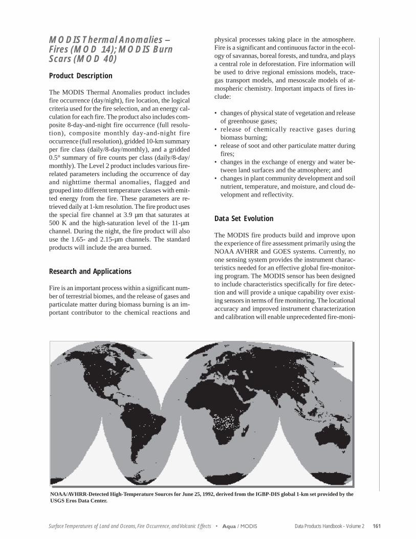
Data Products Handbook - Volume 2 161Surface Temperatures of Land and Oceans, Fire Occurrence, and Volcanic Effects •
MODIS Thermal Anomalies –Fires (MOD 14); MODIS BurnScars (MOD 40)
Product Description
The MODIS Thermal Anomalies product includesfire occurrence (day/night), fire location, the logicalcriteria used for the fire selection, and an energy cal-culation for each fire. The product also includes com-posite 8-day-and-night fire occurrence (full resolu-tion), composite monthly day-and-night fireoccurrence (full resolution), gridded 10-km summaryper fire class (daily/8-day/monthly), and a gridded0.5° summary of fire counts per class (daily/8-day/monthly). The Level 2 product includes various fire-related parameters including the occurrence of dayand nighttime thermal anomalies, flagged andgrouped into different temperature classes with emit-ted energy from the fire. These parameters are re-trieved daily at 1-km resolution. The fire product usesthe special fire channel at 3.9 µm that saturates at500 K and the high-saturation level of the 11-µmchannel. During the night, the fire product will alsouse the 1.65- and 2.15-µm channels. The standardproducts will include the area burned.
Research and Applications
Fire is an important process within a significant num-ber of terrestrial biomes, and the release of gases andparticulate matter during biomass burning is an im-portant contributor to the chemical reactions and
Aqua / MODIS
NOAA/AVHRR-Detected High-Temperature Sources for June 25, 1992, derived from the IGBP-DIS global 1-km set provided by theUSGS Eros Data Center.
physical processes taking place in the atmosphere.Fire is a significant and continuous factor in the ecol-ogy of savannas, boreal forests, and tundra, and playsa central role in deforestation. Fire information willbe used to drive regional emissions models, trace-gas transport models, and mesoscale models of at-mospheric chemistry. Important impacts of fires in-clude:
• changes of physical state of vegetation and releaseof greenhouse gases;
• release of chemically reactive gases duringbiomass burning;
• release of soot and other particulate matter duringfires;
• changes in the exchange of energy and water be-tween land surfaces and the atmosphere; and
• changes in plant community development and soilnutrient, temperature, and moisture, and cloud de-velopment and reflectivity.
Data Set Evolution
The MODIS fire products build and improve uponthe experience of fire assessment primarily using theNOAA AVHRR and GOES systems. Currently, noone sensing system provides the instrument charac-teristics needed for an effective global fire-monitor-ing program. The MODIS sensor has been designedto include characteristics specifically for fire detec-tion and will provide a unique capability over exist-ing sensors in terms of fire monitoring. The locationalaccuracy and improved instrument characterizationand calibration will enable unprecedented fire-moni-

162 Data Products Handbook - Volume 2 • Surface Temperatures of Land and Oceans, Fire Occurrence, and Volcanic Effects
MODIS Sea Surface Temperature(SST) (MOD 28)
Product Description
This Level 2 and 3 product provides sea surface tem-perature at 1-km (Level 2) and 4.6 km, 36 km, and1° (Level 3) resolutions over the global oceans. Inaddition, a quality-assessment parameter is includedfor each pixel. The Level 2 product is produced dailyand consists of global day and night coverage every24 hours. It is used to generate the gridded Level 3products daily, 8-day weekly, monthly, and yearly forday and night conditions. A quality parameter is pro-vided for each data set.
Research and Applications
The global distribution and variability of sea surfacetemperature are key inputs to Earth energy and hy-drological balance studies and long-term climate-change studies. In addition, sea surface temperatureis required by a number of MODIS algorithms in-cluding those for precipitable water, lifted index, wa-ter-leaving radiance, productivity, oceanic aerosolproperties, and temperature and water-vapor profiles.MODIS sea surface temperature retrievals will be in-corporated into a match-up database with radianceand buoy sea surface temperature observations (seeMOD 32).
Data Set Evolution
Sea surface temperature determination is based onMODIS-calibrated mid- and far-IR radiances (Bands20, 22, 23, 31, and 32 from MOD 02), using an algo-rithm that exploits the differences in atmospherictransmissivity in the different IR bands to enablehighly accurate estimation of the atmospheric effects,thereby enabling ancillary input to the algorithmalong with a land mask, which is used to mark non-water pixels while an ice-extent mask limits polarsea coverage. A sequence of spatial and temporalhomogeneity tests is applied to validate the qualityof the cloud-free observations. The AIRS SST esti-mate will be used as a near-real-time quality assess-ment of skin temperature. Visible and near-IR radi-ances (Bands 3, 4, 5, 6) will be used as a secondarycloud flag in the event that the cloud-screening prod-uct is not available.
Aqua / MODIS
toring data sets. The combination of Terra and Aquadata will provide four observations per day, giving agood sampling of the diurnal cycle of fire activity.MODIS will also offer unique spatial and radiomet-ric capabilities for burn-scar detection. Automaticprocedures for burn-scar detection will be developedto provide a standard burn-scar product.
Suggested Reading
Andreae, M.O. et al., 1994.
Justice C.O. et al., 1993.
Justice C.O. et al., 1998.
Kaufman, Y.J. et al., 1990.
Kaufman, Y.J. et al., 1998a.
Levine, J.S., 1991.
Penner, J.E. et al., 1992.
MODIS Thermal Anomalies – Fires and BurnScars Summary
Coverage: Global, daytime/nighttime
Spatial/Temporal Characteristics: 1 km, 10 km,and 0.5°/1-day (MOD 14 only), 8-day,16-day (MOD 40 only), monthly
Key Geophysical Parameters: Fire occurrenceand class, fire selection criteria, fire location,smoldering and flaming ratio, burned area
Processing Level: 2, 3 for MOD 14; 4 forMOD 40
Product Type: Standard, at-launch and post-launch
Maximum File Size: 81 MB (MOD 14), 92 MB(MOD 40)
File Frequency: 1/day (Daily, MOD 14 only),1/8-day (8-day), 1/16-day (16-day, MOD 40only),1/month (Monthly)
Primary Data Format: HDF-EOS
Additional Product Information:http://modis-land.gsfc.nasa.gov/products/products.asp?ProdFamID=1
DAAC: EROS Data Center
Science Team Contacts:Y.J. KaufmanC.O. Justice
(MODIS Thermal Anomalies, continued)

Data Products Handbook - Volume 2 163Surface Temperatures of Land and Oceans, Fire Occurrence, and Volcanic Effects •
Changes in Pacific Sea Surface Temperature (SST) due to El Niño. SST from the NOAA AVHRR, showing patterns before (left) andduring (right) the major 1992 El Niño. The improved accuracy of IR SST products expected from MODIS will enable investigationof the relatively small changes in SST hypothesized to be responsible for triggering El Niño cycles in the Pacific and their ramifica-tions globally. (Note: temperatures range from 20° to 30°C.) (From Brown, O., and G. Feldman, “Reports to the Nation: El Niño andClimate Prediction,” Spring 1994, No. 3, University Corporation for Atmospheric Research, Boulder, CO.)
Aqua / MODIS
Suggested Reading
Abbott, M.R., and D.B. Chelton, 1991.
Barton, I.J. et al., 1989.
Brown, O.B., and R.E. Cheney, 1983.
Deschamps, P., and T. Phulpin, 1980.
Edwards, T. et al., 1990.
Llewellyn-Jones, D.T. et al., 1984.
McClain, E.P. et al., 1985.
Minnett, P.J., 1991.
Minnett, P.J., 1995.
Schluessel, P. et al., 1990.
Smith, A.H. et al., 1994.
Smith, W.L. et al., 1996.
Strong, A.E., and E.P. McClain, 1984.
MODIS Sea Surface Temperature Summary
Coverage: Global ocean surface, clear-skyonly
Spatial/Temporal Characteristics: 1 km/daily(Level 2); 4.6 km, 36 km, 1°/daily, 8-day,monthly, yearly (Level 3)
Key Science Applications: Energy and hydro-logical balance, climate-change models
Key Geophysical Parameters: Sea surfacetemperature
Processing Level: 2, 3
Product Type: Standard, at-launch
Maximum File Size: 33 MB (Level 2); 640 MBbinned, 134 MB mapped (Level 3)
File Frequency: 288/day (Daily Level 2), 4/day(Daily Level 3), 4/8-day (8-day Level 3),4/month (Monthly Level 3), 4/year (YearlyLevel 3)
Primary Data Format: HDF-EOS
Browse Available: 36 km sample imageryavailable at the Goddard DAAC (Level 3only)
Additional Product Information:http://modis-ocean.gsfc.nasa.gov/dataprod.html
DAAC: NASA Goddard Space Flight Center
Science Team Contact:O. Brown

164 Data Products Handbook - Volume 2 • Surface Temperatures of Land and Oceans, Fire Occurrence, and Volcanic Effects Aqua / MODIS
An Example of an 8-day Global Sea Surface Temperature Map generated using data acquired inMarch 2000 from the MODIS instrument on Terra.
(MODIS Sea Surface Temperature, continued)
Sea Surface Temperature off the East Coast of North America, May 8, 2000, derivedfrom data of the MODIS instrument on Terra. This is a Level 2, 1-km resolution prod-uct and shows entrainment of Gulf Stream, shelf, and Sargasso Sea waters into coldand warm core rings.
165
Vegetation Dynamics,Land Cover, andLand Cover Change
Aqua• AMSR-E
• MODIS
Landsat 7*• ETM+
VCL• MBLA
* See Overview Product Description immediately following, and also see chapter on Radiance/Reflectance and Irradiance Products.

166 Data Products Handbook - Volume 2 • Vegetation Dynamics, Land Cover, and Land Cover Change
Vegetation Dynamics, LandCover, and Land Cover Change –An Overview
Relationship to Global Change Issues
In spite of the severe inroads of human constructions,much of the Earth’s land surface remains vegetated,and this vegetation remains critical to the life-sup-port systems of humans and all other land-based ter-restrial animals. Knowledge of vegetation, land coverand land-use change provides the basis for under-standing land and water resource management and arange of research and global monitoring objectives,including global carbon modeling, greenhouse gasemission inventories, regional environment and de-velopment assessments, and forest resource manage-ment. Ecologists and climatologists have developedmodels that describe the matter and energy ex-changes, but lack of long-term global data limits theiruse in Earth system models. Additionally, we lackgood global data on land-surface albedos, on the dis-tribution of soils and important properties of vegeta-tion morphology and physiology, and on water stor-age in soils and snow cover and its relationship torunoff. Incorporation of this information in the land-surface component of climate models will improveestimates of exchanges of water and energy with theatmosphere and lead to more realistic climate simu-lations.
Product Overview – Vegetation
The MODIS land-vegetation products provide infor-mation on terrestrial systems that have important linksto climate and atmospheric composition. These linksare needed for development and application of fullycoupled models of the Earth’s system. They involveexchanges of energy and moisture, radiatively activetrace gases such as carbon dioxide and methane, andphotochemically active species such as nitric oxideand non-methane hydrocarbons, released by soils,plants, and biomass burning.
The MODIS products provide the basic measure-ments of the photosynthetic engines that drive car-bon transport on land. For land areas, vegetation den-sity and vegetation-canopy factors are produced, andthese are used to generate land primary productivity,the amount of carbon fixed by vegetation growth perday or per a longer unit of time such as a year. TheMODIS vegetation measurements are provided bythe Vegetation Indices (MOD 13), Leaf Area Index
(LAI) and Fraction of Photosynthetically Active Ra-diation (FPAR)(MOD 15), and Vegetation CoverConversion (MOD 44) products.
Vegetation indices are radiometric measures of theamount of vegetation present on the ground in a par-ticular pixel. The MODIS indices are obtained frommeasurements of reflected visible and near-infraredenergy from vegetation and are called normalized dif-ference vegetation indices (NDVIs). These indiceshave values between -1 and 1 and increase with in-creasing amounts of vegetation. Several new indiceshave been developed which compensate for soil andatmospheric effects, and these are combined into themodified vegetation index (MVI), also to be producedby MODIS. The indices will be produced at differ-ent resolutions and time-averaging intervals to pro-vide measures of vegetation density and productiv-ity required by global-change models.
The LAI product provides information on the struc-tural property of a plant canopy such as the numberof equivalent layers of leaves the vegetation displaysrelative to a unit ground area. It is derived from thevegetation index. This parameter is an input to thePhotosynthesis and Net Primary Production algo-rithms that produce the global model inputs for land.The FPAR product provides another key input to theproduction algorithm. It measures the proportion ofavailable radiation in the specific photosyntheticallyactive wavelengths of the spectrum that a canopyabsorbs. It is also derived from the vegetation index.These two products provide the vegetation measure-ments that are combined with surface temperatureand radiation inputs in the vegetation-production al-gorithm.
The two primary vegetation products from the VCLmission and its MBLA instrument are geolocatedcanopy-top height and geolocated vertical distribu-tion of intercepted surfaces (VDIS). These are bothLevel 2 products obtained with a spatial resolutionof approximately 25 km. The canopy-top height pro-vides a unique measure of vegetative heights at glo-bal scales and also an indication of above-ground bio-mass. The VDIS provides a new means to classifyvegetation architecture and functions as a predictorof the successional state of a forest.
The ETM+ instrument on Landsat 7 does not di-rectly provide vegetation products in the sense thatthe MODIS instrument on Aqua or the MBLA onVCL do. Rather, calibrated radiances from ETM+ aremade widely available to the scientific communityconcerned with the global distribution and charac-terization of vegetation at higher resolution than pro-vided by MODIS. It is left to the scientific commu-nity to develop specific ETM+ products, which will
Overview

Data Products Handbook - Volume 2 167Vegetation Dynamics, Land Cover, and Land Cover Change •
include maps that quantify land use, land cover, de-forestation, plant biomass, urban sprawl, and ice-sheetdynamics.
Product Overview – Land Cover and LandCover Change
The AMSR-E, MODIS, MBLA, and ETM+ instru-ments will all obtain information of value to studiesof land cover and land cover change, AMSR-E forsoil moisture, MBLA for ground elevations, andMODIS and ETM+ for land cover types.
The AMSR-E soil moisture product obtains a mea-sure of the mean volumetric moisture content in thetop few millimeters of soil, at a 56-km spatial reso-lution. The product is restricted to non-mountainousregions with no snow, low vegetation, and no ongo-ing precipitation. However, in spite of the limitations,AMSR-E is considered the best instrument to datefor satellite sensing of soil moisture. The anticipatedaccuracy of the AMSR-E soil moisture estimates inthe restricted regions of soil moisture retrievals isabout 0.06 g cm-3.
The MBLA ground-elevation measurements willobtain billions of sub-canopy surface elevation points,determined by assuming that the laser waveform’slast return exceeding a set threshold level is theground return. These measurements will provide asignificant advance over current remote sensing to-pographic techniques, none of which is able reliablyto penetrate a canopy-covered surface to obtain ac-curate surface heights.
The MODIS Land Cover Type product (MOD 12)maps global terrestrial land cover at 1-km resolution.The land cover change product will detect areas ofchange and identify types of change processes as theyoccur. Land cover, as well as both human and naturalalteration of land cover, plays a major role in global-scale patterns of climate and biogeochemistry.
The MODIS land cover product will recognize 18basic classes of land cover types, independent of cli-mate. Vegetation classes will separate needleleaf,broadleaf, and graminoid leaf structures; annuallydeciduous and evergreen canopy habitats; and sparse-to-dense-cover fractions following the InternationalGeosphere-Biosphere Programme (IGBP) scheme.Also, major classes of agricultural activities will berecognized as well as several categories of land sur-faces with little or no plant cover, such as bare sand,soil, or rock.
The MODIS land cover product will detect and cat-egorize changes in terrestrial features and processeson a global scale. Independent of the land cover prod-
Overview
uct, the land-cover-change algorithm will compare,pixel-by-pixel, the temporal development curve of aset of biophysical and spatial indicators derived fromMODIS data.
As indicated above, the ETM+ instrument on Land-sat 7 will not directly be the source of land-cover andland-cover-change products, but rather will be thesource of calibrated radiances at 30-m resolution andat seven spectral bands that will make it possible formembers of the scientific community worldwide toapply their own algorithms to develop products thatdefine land cover and land cover change on a globalbasis.
Product Interdependency and Continuitywith Heritage Data
The MODIS land products flow in a chain from theLevel 2 reflectance and land cover type parametersto biophysical- and biochemical-derived productsused as inputs to Earth system models. Specific prod-uct dependencies for the land vegetation indices areMODIS radiance and imagery products, includingLevel 1B calibrated radiance, surface-leaving radi-ance, and aerosol optical depth. The vegetation in-dex is the key input to Leaf Area Index and FPARproducts, which are the key inputs along with landcover type into the biomass-product algorithm.
Each MODIS product has its own science require-ments and objectives and builds on the heritage ofproducts produced for many years from AVHRR andother data sets. MODIS will produce a “continuity”NDVI to maintain the AVHRR NDVI time series us-ing an algorithm that closely approximates the heri-tage index. A worldwide database has been createdwith the AVHRR data, and EOS will continue thisseries.
The products that will come into being as a resultof analysis of the calibrated radiances from ETM+will continue the long heritage of measurements thatextend back to the Landsat 1 satellite, launched in1972. Despite improvements in Landsat through thedevelopment of ETM+, continuity has been main-tained with the original measurements from Landsat1 and with the spectral enhancements added toLandsats 4 and 5. Improvements incorporated in theLandsat 7 sensor include a 15-m panchromatic band,superior spatial resolution for the thermal band (60versus 120 m), and two solar calibrators.
Landsats 2 and 3, launched in 1975 and 1978 re-spectively, were configured similarly. In 1984, Land-sat 4 was launched with the MSS and a new instru-ment called the Thematic Mapper (TM). Instrument

168 Data Products Handbook - Volume 2 • Vegetation Dynamics, Land Cover, and Land Cover Change Overview
upgrades included improved ground resolution (30m) and 3 new channels, or bands. In addition to us-ing an updated instrument, Landsat 4 made use ofthe multimission modular spacecraft (MMS), whichreplaced the Nimbus-based spacecraft design em-ployed for Landsats 1-3. Landsat 5, a duplicate ofLandsat 4, was launched in 1984 and continued re-turning useful data in the late 1990s, far beyond its5-year design life. Landsat 6, equipped with a 15-mpanchromatic band, was lost immediately after launchin 1993.
Suggested Reading
Asrar, G., 1989.
Lambin, E.F., and A.H. Strahler, 1994a,b.
Los, S.O. et al., 1994.
Moody, A., and C. E. Woodcock, 1995.
Nemani, R.R., and S.W. Running, 1995.
Nyoku, E., and L. Li, 1999.
Oliver, C.D., and B.C. Larson, 1990.
Rencz, A., 1999.
Running, S.W. et al., 1994.
Sellers, P.J., 1987.
Ustin, S.L. et al., 1993.
van Leeuwen, W.J.D. et al., 1999.
Vonder, O.W., and J.P.G.W. Clevers, 1998.
Vorosmarty, C. et al., 1991.
(Vegetation Dynamics, Land Cover, and Land Cover Change –An Overview, continued)

Data Products Handbook - Volume 2 169Vegetation Dynamics, Land Cover, and Land Cover Change •
AMSR-E Surface Soil Moisture
Product Description
This Level 2 and 3 product provides surface soilmoisture at 56-km resolution on a nominal 25-kmEarth-registered grid. Gridded brightness tempera-tures are also provided at Level 3. Quality-controlindices and surface-type classification are included.The product spatial resolution is determined by thesensor resolution at the lowest frequency used in theretrievals (6.9 GHz). Surface soil moisture is definedas the mean volumetric moisture content (g cm-3) inthe top few millimeters of soil, or skin depth, aver-aged over the retrieval resolution. In regions of mod-erate-to-dense vegetation cover, snow, frozen ground,precipitation, open water, or mountainous terrain, soilmoisture retrievals are not made. The accuracy of thesoil-moisture retrievals is best for bare soils, andworsens as the vegetation cover increases. Surfacetemperature and vegetation water content are re-trieved simultaneously with the soil moisture and areincluded in the product. The Level 2 product is pro-vided in ascending and descending swath segments.The Level 3 product is generated by compositing theascending and descending Level 2 products into dailyglobal maps.
Research and Applications
Water and energy fluxes at the land-atmosphere in-terface are influenced to a large extent by the surfacesoil moisture. Satellite-derived information on soilmoisture and its variability is thus important for mod-eling surface hydrologic processes, for enabling im-proved weather and climate prediction, and for moni-toring floods, droughts, and vegetation status on aglobal basis.
Data Set Evolution
Soil-moisture remote sensing requires measurementsat long wavelengths to penetrate vegetation cover,and large antennas to provide adequate spatial reso-lution. The AMSR-E is the best instrument to datefor this purpose, with a lowest frequency of 6.9 GHzand a spatial resolution of 56 km at this frequency.The AMSR-E goal is to obtain soil-moisture estimateswith an accuracy of ~0.06 g cm-3 in regions with veg-etation water content of less than ~1.5 kg m-2. Noadequate satellite soil-moisture data sets currently ex-ist. The AMSR-E soil-moisture data set is producedusing algorithms developed from field-experiment
data using airborne and ground-based instrumenta-tion and from historical Nimbus 7 SMMR data analy-sis.
Suggested Reading
Njoku, E.G., and D. Entekhabi, 1996.
Njoku, E., and L. Li, 1999.
Wang, J.R., and B.J. Choudhury, 1995.
AMSR-E Surface Soil Moisture Summary
Coverage: Global land surface, although onlyunder snow-free and low-vegetation con-ditions
Spatial/Temporal Characteristics: 56-km spatialresolution on a nominal 25-km Earth-fixedgrid; swath (Level 2) and daily (Level 3) as-cending and descending
Key Science Applications: Hydrological processes,climate modeling and monitoring
Key Geophysical Parameters: Surface soil mois-ture
Processing Level: 2, 3
Product Type: Standard, at-launch
Maximum File Size: 0.5 MB
File Frequency: 29/day
Primary Data Format: HDF-EOS
Browse Available: Accompanies data product
Additional Product Information:http://wwwghcc.msfc.nasa.gov/AMSR/html/amsr_products.html
DAAC: National Snow and Ice Data Center
Science Team Contact:E.G. Njoku
Aqua / AMSR-E

170 Data Products Handbook - Volume 2 • Vegetation Dynamics, Land Cover, and Land Cover Change Aqua / MODIS
MODIS Surface Reflectance; AtmosphericCorrection Algorithm Products Summary
Coverage: Global land surface (Level 2)
Spatial/Temporal Characteristics: Bands 1 and2, 250 m; bands 3-7, 500 m; daylight dataonly
Key Science Applications: Global climatemodeling, regional climate modeling,surface-energy-balance modeling, landcover characterization
Key Geophysical Parameters: Surface reflec-tance
Processing Level: 2
Product Type: Standard, at-launch
Maximum File Size: 424 MB
File Frequency: 288/day
Primary Data Format: HDF-EOS
Additional Product Information:http://modis-land.gsfc.nasa.gov/mod09/
DAAC: EROS Data Center
Science Team Contact:E. Vermote
MODIS Surface Reflectance;Atmospheric CorrectionAlgorithm Products (also calledSpectral Reflectance) (MOD 09)
Product Description
The MODIS Surface-Reflectance Product (MOD 09)is computed from the MODIS Level 1B land bands1, 2, 3, 4, 5, 6, and 7 (centered at 648 nm, 858 nm,470 nm, 555 nm, 1240 nm, 1640 nm, and 2130 nm,respectively). The product is an estimate of the sur-face spectral reflectance for each band as it wouldhave been measured at ground level if there were noatmospheric scattering or absorption.
The correction scheme includes corrections for theeffect of atmospheric gases, aerosols, and thin cirrusclouds; it is applied to all noncloudy MOD 35Level 1B pixels that pass the Level 1B quality con-trol. The correction uses band 26 to detect cirruscloud, water vapor from MOD 05, aerosol from MOD04, and ozone from MOD 07; best-available clima-tology is used if the MODIS water vapor, aerosol, orozone products are unavailable. Also, the correctionuses MOD 43, BRDF without topography, from theprevious 16-day time period for the atmosphere-BRDF coupling term.
Research and Applications
The surface-reflectance product is the input for prod-uct generation for several land products: VegetationIndices (VIs), BRDF, thermal anomaly, snow/ice, andFraction of Photosynthetically Active Radiation/LeafArea Index (FPAR/LAI). It is, therefore, an impor-tant and essential product. The at-launch version willbe fully operational.
Data Set Evolution
The Aqua MODIS product will be based upon thelatest version of the Terra MODIS product.
Suggested Reading
Vermote, E.F. et al., 1997.

Data Products Handbook - Volume 2 171Vegetation Dynamics, Land Cover, and Land Cover Change •
Research and Applications
This product is used for biophysical and bio-geochemical parameterization of land cover for in-put to global- and regional-scale models of climate,hydrologic processes, and biogeochemical cycling.Examples of biogeophysical parameters keyed to landcover include leaf-area index, vegetation density, andFPAR. Other parameters are biomass permanence andenergy-transfer characteristics of the land surface.
Data Set Evolution
Recent attempts to produce regional-scale land coverdatasets use coarse spatial resolution and high-tem-poral-frequency data from the AVHRR instrumentaboard the NOAA series of meteorological satellites.Most of these efforts have used the Normalized Dif-ference Vegetation Index (NDVI) parameter derivedfrom these data. The NDVI generally quantifies thebiophysical activity of the land surface and as suchdoes not provide land cover directly. The MODISland cover algorithm draws from information do-mains well beyond those used in these efforts includ-ing directional surface reflectance, texture, vegeta-tion index, acquisition geometry, land-surfacetemperature, and snow/ice cover derived from theMODIS instruments on both Terra and Aqua. Thealgorithm will use a hybrid decision-tree neural-net-work classifier. Product validation will be based on anetwork of about 400 test sites. High-resolution im-agery (e.g., Landsat) will be used to establish truth
MODIS Land Cover Type(MOD 12)
Product Description
This Level 3 product contains land cover type andland cover change parameters, which will be pro-duced at 1-km resolution on a quarterly basis begin-ning 18 months following launch of the Terra andAqua platforms. In the period 6-18 months afterlaunch, prototype products will be made available.The land cover parameter identifies 17 categories ofland cover following the IGBP global vegetation da-tabase, which defines nine classes of natural vegeta-tion, three classes of developed lands, two classes ofmosaic lands, and three classes of nonvegetated lands(snow/ice, bare soil/rocks, water). The land coverchange parameter quantifies subtle and progressiveland-surface transformations as well as major rapidchanges. As such, it is not a conventional changeproduct that only compares changes in land covertype at two times but combines analyses of changein multispectral-multitemporal data vectors withmodels of vegetation-change mechanisms to recog-nize both the type of change and its intensity. It willhighlight interannual variability in particular. In ad-dition to the basic 1-km product, summary productscontaining proportions of land covers and changecharacteristics will be available at one-quarter, one-half, and 1-degree resolutions. These products are pre-pared independently from the 250-m Land CoverChange Product and use a different algorithm.
Aqua / MODIS
1. Evergreen Needleleaf Forest2. Evergreen Broadleaf Forest4. Deciduous Broadleaf Forest5. Mixed Forests8. Woody Savannahs9. Savannahs10. Grasslands12. Croplands13. Urban and Built14. Cropland/Natural Vegetation Mosaic17. Water Bodies
Scale 1:6,000,000
0 200Boston University Center for Remote Sensing
Land Cover Classes in a Mid-Atlantic Subset of the North American Prototype of the MODIS Land CoverProduct, September 1999.
km

172 Data Products Handbook - Volume 2 • Vegetation Dynamics, Land Cover, and Land Cover Change Aqua / MODIS
(MODIS Land Cover Type, continued)
for the sites, which will be used to train the land-cover classifier and validate the products. The vali-dation procedure will characterize the accuracy ofthe product as well as provide information that canbe used in spatial aggregation to provide land coverdata and land cover change data at coarser resolu-tions.
Suggested Reading
Justice, C. et al., 1998.
Running, S.W. et al., 1994.
Running, S.W. et al., 1995.
Salisbury, J.W., and D.M. D’Aria, 1992.
Snyder, W., and Z. Wan, 1996.
Strahler, A. et al., 1995.
Wan, Z., and J. Dozier, 1996.
Wan, Z., and Z.-L. Li, 1997.
MODIS Land Cover Type Summary
Coverage: Global, clear-sky only
Spatial/Temporal Characteristics: 1 km, 1/4°,1/2°, 1°/seasonal (96-day)
Key Science Applications: Biogeochemicalcycles, land cover change
Key Geophysical Parameters: Land cover type,land cover change
Processing Level: 3
Product Type: Standard, post-launch
Maximum File Size: 16 MB
File Frequency: 289/96-day
Primary Data Format: HDF-EOS
Additional Product Information:http://modis-land.gsfc.nasa.gov/products/products.asp?ProdFamID=10
DAAC: EROS Data Center
Science Team ContactA.H. Strahler

Data Products Handbook - Volume 2 173Vegetation Dynamics, Land Cover, and Land Cover Change •
MODIS Vegetation Indices(MOD 13)
Product Description
The MODIS Vegetation-Index (VI) products will pro-vide consistent spatial and temporal comparisons ofglobal vegetation conditions that will be used to moni-tor the Earth’s terrestrial photosynthetic vegetationactivity in support of change detection and pheno-logic and biophysical interpretations. Gridded veg-etation-index maps depicting spatial and temporalvariations in vegetation activity are derived at 8-day,16-day, and monthly intervals for precise seasonaland interannual monitoring of the Earth’s vegetation.The MODIS VI products will improve upon currentlyavailable indices and will more accurately monitorand detect changes in the state and condition of theEarth’s vegetative cover. The vegetation-index prod-ucts are made globally robust with enhanced vegeta-tion sensitivity and minimal variations associatedwith external influences (atmosphere, view and sunangles, clouds) and inherent, non-vegetation influ-ences (canopy background, litter), in order to servemore effectively as a “precise” measure of spatialand temporal vegetation change.
Two vegetation-index (VI) products are to be pro-duced globally for land at launch. One is the stan-dard normalized difference vegetation index (NDVI),which is referred to as the “continuity index” to theexisting NOAA-AVHRR-derived NDVI. The otheris an enhanced vegetation index (EVI) with improvedsensitivity in high biomass regions and improved veg-etation monitoring through a decoupling of thecanopy background signal and a reduction in atmo-sphere influences. The two VIs complement eachother in global vegetation studies and improve uponthe extraction of canopy biophysical parameters. Anew compositing scheme that reduces angular, sun-target-sensor variations is also utilized. The griddedvegetation-index maps will use as input MODIS Terraand Aqua surface reflectances, corrected for molecu-lar scattering, ozone absorption, and aerosols, andadjusted to nadir and standard sun angles with use ofBRDF models. The gridded vegetation indices willinclude quality-assurance (QA) flags with statisticaldata, indicating the quality of the VI product and in-put data. The MODIS vegetation-index products willinclude:
• 250-m NDVI and QA as 8-day, 16-day, andmonthly products (high resolution)
• 1-km NDVI, EVI, and QA as 8-day, 16-day, andmonthly products (standard resolution)
• 25-km NDVI, EVI, and QA as 8-day, 16-day, andmonthly products (coarse resolution)
Research and Applications
Due to their simplicity, ease of application, and wide-spread familiarity, vegetation indices are widely usedby the broader user community from global circula-tion climate modelers and EOS instrument teams andinterdisciplinary projects in hydrology, ecology, andbiogeochemistry to those making regional- and glo-bal-based applications involving natural-resource in-ventories, land-use planning, agricultural monitoringand forecasting, and drought forecasting. Some ofthe more common applications of the vegetation in-dex concern:
• Global warming/climate• Global biogeochemical and hydrologic modeling• Agriculture; precision agriculture; crop stress, crop
mapping• Rangelands; water supply forecasting; grazing ca-
pacities; fuel supply• Forestry, deforestation, and net primary produc-
tion studies• Pollution/health issues (Rift valley fever, mosquito-
producing rice fields)• Desertification• Anthropogenic-change detection and landscape
disturbances.
Data Set Evolution
At the time of the launch of Aqua, there will be a 20-year NDVI global data set (1981-2000) from theNOAA- AVHRR series, which could be extended byMODIS Terra and Aqua data to provide a long-termdata record for use in operational monitoring stud-ies. The MODIS Terra and Aqua data set can readilybe composited to provide 16-day, cloud-free time-series maps of vegetation activity. When both Terraand Aqua data are combined, higher frequency, 8-day, cloud-free time-series data will be readily madeavailable.
Aqua / MODIS

174 Data Products Handbook - Volume 2 • Vegetation Dynamics, Land Cover, and Land Cover Change
(MODIS Vegetation Indices, continued)
Suggested Reading
Cihlar, J.C. et al., 1997.
Huete, A.R. et al., 1994.
Huete, A.R. et al., 1997.
Huete, A.R. et al., 1999.
Myneni, R.B. et al., 1997a,b.
van Leeuwen, W.J.D. et al., 1999.
MODIS Vegetation Indices Summary
Coverage: Global land surface
Spatial/Temporal Characteristics: 250 m, 1 km,and 0.25° resolutions/8-day, 16-day, andmonthly
Key Science Applications: Global vegetationmonitoring, biogeochemical and hydro-logic modeling, health and food security,range and forestry monitoring, agricul-ture management
Key Geophysical Parameters: Vegetationindices (NDVI & EVI)
Processing Level: 2,3
Product Type: Standard, at-launch
Maximum File Size: 277 MB
File Frequency: 289/16-day (16-day),289/month (Monthly)
Primary Data Format: HDF-EOS
Additional Product Information:http://modis-land.gsfc.nasa.gov/products/products.asp?ProdFamID=6
DAAC: EROS Data Center
Science Team Contact:A.R. Huete
Aqua / MODIS

Data Products Handbook - Volume 2 175Vegetation Dynamics, Land Cover, and Land Cover Change •
High Resolution (1 km) Composite of MODIS Enhanced Vegeta-tion Index (top) and Normalized Difference Vegetation Index (bot-tom) for North America, from data of the Terra MODIS instru-ment for March 5 - March 20, 2000.
High Resolution (500 m) Composite of the Normal-ized Difference Vegetation Index for North and SouthAmerica, from data of the Terra MODIS instrumentfor April 22 - May 7, 2000.
Global Composite of MODISEnhanced Vegetation Index(top) and Normalized Differ-ence Vegetation Index (bot-tom), both from data of theTerra MODIS for March 17- April 2, 2000.
Aqua / MODIS

176 Data Products Handbook - Volume 2 • Vegetation Dynamics, Land Cover, and Land Cover Change
MODIS Leaf Area Index (LAI)and Fraction ofPhotosynthetically ActiveRadiation (FPAR) – ModerateResolution (MOD 15)
Product Description
The MOD 15 Leaf Area Index (LAI) and Fraction ofPhotosynthetically Active Radiation absorbed byvegetation (FPAR) are 1-km at-launch products pro-vided on a daily and 8-day basis. LAI defines an im-portant structural property of a plant canopy, namelythe one-sided leaf area per unit ground area. FPARmeasures the proportion of available radiation in thephotosynthetically active wavelengths (400 to 700nm) that a canopy absorbs. The LAI product will bea LAI value between 0 and 8 of the global griddeddatabase at the corresponding modified vegetationindex (MVI) compositing interval. The FPAR prod-uct will be an FPAR value between 0.0 and 1.0 as-signed to each 1-km cell of the global gridded data-base at the corresponding MVI compositing interval.
Research and Applications
LAI and FPAR are biophysical variables that describecanopy structure and are related to functional pro-cess rates of energy and mass exchange. Both LAIand FPAR have been used extensively as satellite-derived parameters for calculation of surface photo-synthesis, evapotranspiration, and NPP. These prod-ucts are essential in calculating terrestrial energy,carbon, water-cycle processes, and biogeochemistryof vegetation. The LAI product is an input to Biome-BGC (Biogeochemical) models to produce conver-sion-efficiency coefficients, which are combined withthe FPAR product to produce daily terrestrial PSN(photosynthesis) and annual NPP.
Data Set Evolution
This product is derived from the Surface ReflectanceProduct (MOD 09), the Land Cover Type product(MOD 12), and ancillary information on surface char-acteristics such as land cover type and background.The retrievals are performed by comparing observedand modeled surface reflectances for a suite of canopystructures and soil patterns that covers a range of ex-pected natural conditions. All canopy/soil patterns forwhich the magnitude of the residuals in the compari-
son does not exceed uncertainties in observed andmodeled surface reflectances are treated as accept-able solutions. For each acceptable solution, a valueof FPAR is also evaluated. The mean and dispersionvalues of the LAI solution distribution function aretaken as the retrieved LAI accuracy; likewise forFPAR. A three-dimensional formulation of the radia-tive transfer is used to derive spectral and angularbiome-specific signatures of vegetation canopies.Should this main algorithm fail, a back-up algorithmis triggered to estimate LAI and FPAR using a Nor-malized Difference Vegetation Index (NDVI).
Suggested Reading
Knyazikhin, Y. et al., 1998a.
Knyazikhin, Y. et al., 1998b.
Myneni, R.B. et al., 1997b.
Tian, Y. et al., 2000.
Zhang, Y. et al., 2000.
MODIS LAI and FPAR – Moderate ResolutionSummary
Coverage: Global
Spatial/Temporal Characteristics: 1 km/daily,8-day
Key Science Applications: Biogeochemical cyclemodeling, NPP estimation
Key Geophysical Parameters: Leaf area index,fraction of photosynthetically activeradiation absorbed by vegetation
Processing Level: 4
Product Type: Standard, at-launch
Maximum File Size: 5.8 MB
File Frequency: 289/day (Daily Level 4),289/8-day (8-day Level 4)
Primary Data Format: HDF-EOS
Additional Product Information:http://modis-land.gsfc.nasa.gov/products/products.asp?ProdFamID=5
DAAC: EROS Data Center
Science Team Contacts:R.B. MyneniS.W. Running
Aqua / MODIS
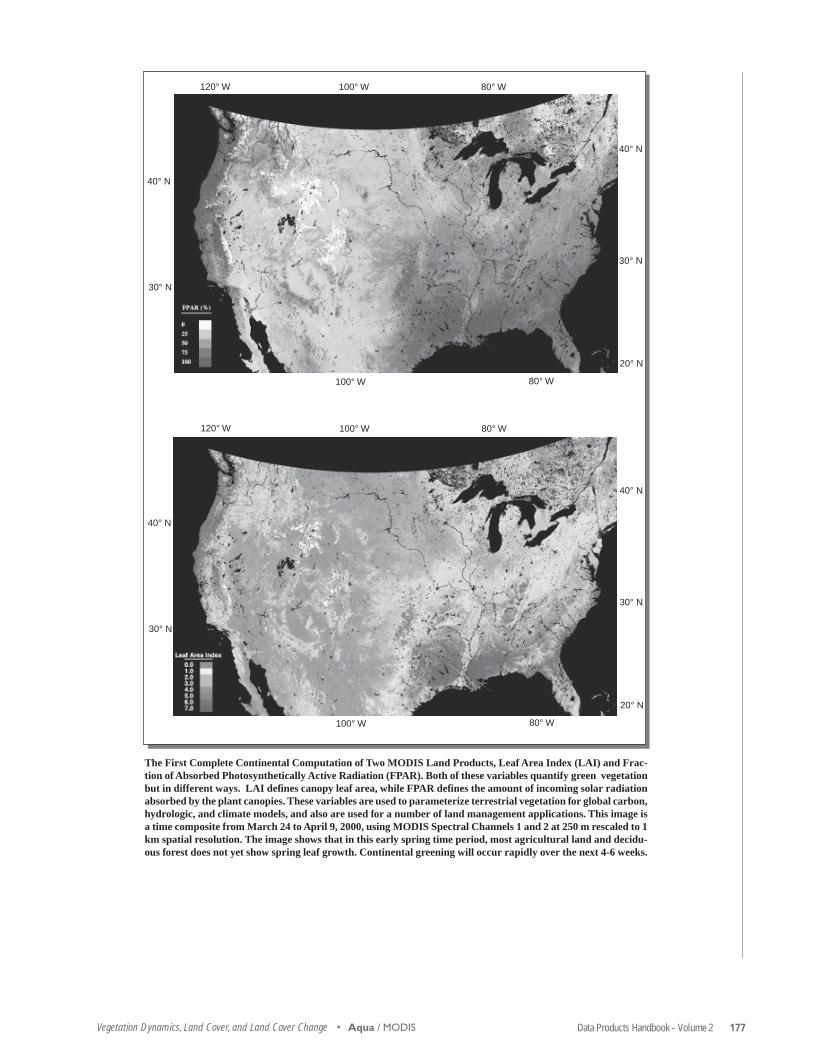
Data Products Handbook - Volume 2 177Vegetation Dynamics, Land Cover, and Land Cover Change • Aqua / MODIS
40° N
30° N
120° W 100° W 80° W
40° N
30° N
20° N
100° W 80° W
40° N
30° N
120° W 100° W 80° W
40° N
30° N
20° N
100° W 80° W
The First Complete Continental Computation of Two MODIS Land Products, Leaf Area Index (LAI) and Frac-tion of Absorbed Photosynthetically Active Radiation (FPAR). Both of these variables quantify green vegetationbut in different ways. LAI defines canopy leaf area, while FPAR defines the amount of incoming solar radiationabsorbed by the plant canopies. These variables are used to parameterize terrestrial vegetation for global carbon,hydrologic, and climate models, and also are used for a number of land management applications. This image isa time composite from March 24 to April 9, 2000, using MODIS Spectral Channels 1 and 2 at 250 m rescaled to 1km spatial resolution. The image shows that in this early spring time period, most agricultural land and decidu-ous forest does not yet show spring leaf growth. Continental greening will occur rapidly over the next 4-6 weeks.

178 Data Products Handbook - Volume 2 • Vegetation Dynamics, Land Cover, and Land Cover Change
MODIS Surface Resistance andEvapotranspiration (MOD 16)
Product Description
This Level 4 product consists of Surface Resistanceand Evapotranspiration (ET) parameters and has atemporal resolution of eight days at a spatial resolu-tion of 1 km over the land surface only. The landSurface Resistance is an Aqua product that capturessub-optimum conditions produced by soil/atmo-spheric moisture deficits for vegetation photosynthe-sis and transpiration. The spatial resolution of theseproducts is 1 km.
Research and Applications
These two parameters are essential to global model-ing of climate, water balance, and trace gases. In ad-dition, they are required in estimating photosynthe-sis, respiration, and net primary production. Thesurface-resistance product is an Aqua (post-launch)research data product intended for real-time imple-mentations. Practical applications of this product arefor monitoring wildfire danger and crop/rangedrought.
Data Set Evolution
The Surface Resistance product will be calculatedusing the MODIS Land Surface Temperature (MOD11) and the MODIS modified vegetation index (MOD13), and will be used along with incident radiationfor computing the ET.
Suggested Reading
Dickinson, R.E., 1987.
Goward, S.N., and A.S. Hope, 1989.
Nemani, R.R., and S.W. Running, 1989.
Nemani, R.R. et al., 1993.
Running, S.W. et al., 1989.
Running, S.W. et al., 1994.
MODIS Surface Resistance andEvapotranspiration Summary
Coverage: Global
Spatial/Temporal Characteristics: 1 km/8-day,yearly
Key Science Applications: Global water balance,net primary production
Key Geophysical Parameters: Surface resis-tance, evapotranspiration
Processing Level: 4
Product Type: Research, post-launch
Maximum File Size: 5.8 MB
File Frequency: 289/8-day
Primary Data Format: HDF-EOS
Additional Product Information:http://modis-land.gsfc.nasa.gov/products/products.asp?ProdFamID=3
DAAC: EROS Data Center
Science Team Contact:S.W. Running
Aqua / MODIS

Data Products Handbook - Volume 2 179Vegetation Dynamics, Land Cover, and Land Cover Change • Aqua / MODIS
MODIS Vegetation Productionand Net Primary Production(MOD 17)
Product Description
MOD 17 is a Level 4 product consisting of 8-dayNet Photosynthesis (PSN) and Net Primary Produc-tion (NPP). Annual NPP is the time integral of thePSN product over a year.
Research and Applications
This product provides an accurate measure of terres-trial vegetation growth and production activity. Thetheoretical use is to define the seasonally dynamicflux of terrestrial-surface carbon dioxide for climatemodeling. Fluxes will be computed specific to eachvegetation type. The practical utility is to measurecrop yield and forest production and any other so-cially significant products of vegetation growth. Asthis global NPP product becomes regularly available,a wide variety of derived products is expected to bedeveloped making regionally specific estimates ofcrop production. The value of an unbiased, regularsource of crop and forest production estimates forglobal political and economic decision making isimmense.
Data Set Evolution
The NPP parameter is the yearly integral of the PSNwhich is obtained from the product of PAR (Photo-synthetically Active Radiation), FPAR (Fraction ofPhotosynthetically Active Radiation) and conversion-efficiency coefficients obtained from other MODISproducts and other sensors and ancillary data. Thealgorithms for these products are based on the origi-nal logic of Monteith (1972), which relates PSN andNPP to the amount of Absorbed PhotosyntheticallyActive Radiation (APAR). The MODIS modifiedvegetation indices (MVI) along with climate variablesand the land cover product are used to estimate APAR.
Suggested Reading
Field, C.B. et al., 1995.
Monteith, J.L., 1972.
Prince, S.D., and S.N. Goward, 1995.
Ruimy, A. et al., 1994.
Running, S.W., 1990.
Running, S.W. et al., 1994.
MODIS Vegetation Production and NetPrimary Production Summary
Coverage: Global
Spatial/Temporal Characteristics: 0.5, 1, 10 km/8-day, yearly
Key Science Applications: Interannual variabil-ity of vegetation
Key Geophysical Parameters: NPP, photosyn-thesis, respiration
Processing Level: 4
Product Type: Standard, at-launch
Maximum File Size: 4.3 MB
File Frequency: 289/8-day
Primary Data Format: HDF-EOS
Additional Product Information:http://modis-land.gsfc.nasa.gov/products/products.asp?ProdFamID=3
DAAC: EROS Data Center
Science Team Contact:S.W. Running

180 Data Products Handbook - Volume 2 • Vegetation Dynamics, Land Cover, and Land Cover Change
<0.1
0.1-0.5
0.5-1.0
1.0-1.5
1.5-2.0
2.0-2.5
>2.5
(kg/m2/yr)
Resolution 1°×1° Lat/Lon
neman/hunt/running/NTSG
Global Net Primary Production (NPP) during 1987. This data set is produced using 1° × 1° gridded climate data from 7000 weatherstations distributed globally, Mathews land cover classes collapsed into six classes, biome-specific NDVI-LAI relations used to estimateLAI from NOAA/NASA Pathfinder data, and an ecosystem simulation model, BIOME-BGC.
Aqua / MODIS
quantify the directional information in the remotely-sensed signal, which is related to ground-cover type;and 3) provide a surface-radiation-scattering modelfor boundary-layer parameterization in regional andglobal climate modeling. The BRDF can also be usedin extraction of surface reflectances at Level 2. Twoalbedo measures are provided: “black-sky” albedo(directional-hemispherical reflectance) and “white-sky” albedo (bihemispherical reflectance). These areintrinsic surface properties, independent of atmo-spheric state. They describe the upward scattering ofthe solar beam and of uniform diffuse irradiance, re-spectively, and may be used as input to global andregional climate models.
Data Set Evolution
The BRDF/Albedo algorithm combines gridded,multidate, multiband surface-reflectance data fromEOS MODIS and MISR (on Terra) instruments toproduce BRDF functions and derived albedo mea-sures. For each grid cell, all cloud-free observationsin a 16-day period are assembled and fit to the Ross-Thick/Li-Sparse semiempirical model that describesthe BRDF as a linear function of two basic BRDFshapes. In addition, a single empirical model (modi-fied Walthall) is currently also fitted. The algorithmoutputs include: 1) Ross-Thick/Li-Sparse BRDF pa-
MODIS Surface ReflectanceBRDF/Albedo Parameter(MOD 43)
Product Description
The Bidirectional Reflectance Distribution Function(BRDF)/Albedo parameter provides: 1) coefficientsfor mathematical functions that describe the BRDFof each pixel in the seven MODIS “Land” bands (1-7); and 2) albedo measures derived simultaneouslyfrom the BRDF for bands 1-7 as well as three broadbands (0.4-0.7, 0.7-3.0, and 0.4-3.0 micrometers).
Because deriving BRDF and albedo requires merg-ing multiple looks at each pixel, the BRDF/Albedoparameter is provided every 16 days. Its spatial reso-lution is 1 km, gridded to Level 3. A 32-day sum-mary albedo product at 0.25° spatial resolution is alsoprovided. Both Terra and Aqua data are merged asavailable.
Research and Applications
The BRDF functions provided by the BRDF/Albedoparameter: 1) allow normalization of MODIS data tostandard viewing and illumination angles, thus re-moving geometric effects from multidate images; 2)

Data Products Handbook - Volume 2 181Vegetation Dynamics, Land Cover, and Land Cover Change •
rameters that best fit the observations, 2) modifiedWalthall parameters, 3) black-sky and white-sky al-bedos in three broad bands, and 4) nadir BRDF-ad-justed reflectances (NBARs).
Suggested Reading
Barnsley, M.J., and J.-P. Muller, 1991.
d’Entremont, R.E. et al., 1999.
Hu, B. et al., 1997.
Hu, B. et al., 1999.
Hu, B. et al., 2000.
Justice, C. et al., 1998.
Li, X. et al., 1995.
Liang, S. et al., 1999
Lucht, W., 1998.
Lucht, W., and P. Lewis, 2000.
Lucht, W. et al., 2000.
Wanner, W. et al., 1995.
Wanner, W. et al., 1997.
Aqua / MODIS
MODIS Surface Reflectance BRDF/AlbedoParameter Summary
Coverage: Global land surface
Spatial/Temporal Characteristics: 1 km,16 km, 0.5°/16-day; 0.25°/32-day
Key Science Applications: Biogeochemical-cycle modeling, net primary productivityestimation, global climate models
Key Geophysical Parameters: Bidirectionalreflectance, spectral albedo
Processing Level: 3
Product Type: Standard, at-launch
Maximum File Size: 329 MB (16-day),946 MB (32-day)
File Frequency: 289/16-day (16-day),1/month (32-day)
Primary Data Format: HDF-EOS
Additional Product Information:http://modis-land.gsfc.nasa.gov/products/products.asp?ProdFamID=2
DAAC: EROS Data Center
Science Team ContactA.H. StrahlerJ.-P. Muller
Bihemispherical Albedo (White-Sky Albedo) for North America for the pe-riod April 22 - May 7, 2000, calculated from the MODIS BRDF/Albedoproduct algorithm using data from the Terra MODIS near-infrared chan-nel (Band 2). In this image, cloud cover has obscured some regions in thecentral U.S. as well as other smaller areas shown in white. Light tones in thesoutheastern U.S. indicate strong reflectance from leaf cover, while much ofthe more northern regions remains leafless.

182 Data Products Handbook - Volume 2 • Vegetation Dynamics, Land Cover, and Land Cover Change
MODIS Vegetation CoverConversion (MOD 44)
Product Description
Using MODIS data from the two 250-m bands, thevegetation cover conversion product will show theglobal distribution of the occurrence of vegetationcover change. Where there is sufficient evidence, thetype of change will be labeled (e.g., forest conver-sion to agricultural fields or grassland or bare sur-face). The distribution of these changes will be rep-resented at a resolution of 250 meters and as gridded10-km summaries. These will be generated at 3-month intervals. An interannual product is also be-ing produced, displaying the global distribution ofvegetation-cover change during the previous year.
Research and Applications
Vegetation-cover change is an important driver ofmany important biogeochemical, hydrological, andclimate processes. It also represents the integratedresponse to several biophysical and anthropogenicimpacts. Among the important influences of vegeta-tion-cover change are the following:
• It strongly affects changes in many biophysical fac-tors such as surface roughness and albedo;
• It has a major effect on changes in sensible heatflux, because it affects global albedo and surfaceroughness, which in turn affects atmospheric drag;
• It is of crucial importance for determining the bio-geochemical cycling of carbon, nitrogen, and otherelements at regional-to-global scales;
• It has a major impact on the runoff characteristicsof catchments through its effects on evapotranspi-ration and partitioning of precipitation into over-land flow, interflow, and groundwater accretion;
• It gives a direct insight into ecosystem responserelated to climate change and anthropogenic influ-ences;
• It affects biodiversity through direct impacts onhabitat;
• It provides increasingly important information fornatural-resource managers.
This product will be combined with data obtainedfrom finer spatial resolution data from sensors suchas ETM+ on Landsat 7 and ASTER on Terra (seeVolume 1) to assist in the identification of the typesof vegetation conversion occurring. The product alsoprovides information to assist the acquisition strat-
egy of finer resolution systems since it helps flag ar-eas where significant changes are likely to be occur-ring.
Data Set Evolution
Previous work has shown that data with a resolutionof 1 km and coarser are sufficient for the mapping ofthe distribution of vegetation cover and for the moni-toring of those changes in vegetation cover causedby seasonal-to-interannual climate change. However,such relatively coarse resolution data are often inad-equate to detect changes caused by anthropogenicfactors. Analyses of many types of vegetation-coverchange indicate that they are relatively small in sizelargely due to the inherently local nature of anthro-pogenic vegetation-cover conversions. Consequentlya very large proportion of changes is only detectableat fine spatial resolutions. For this reason it was de-cided to use the two 250-m bands for the identifica-tion and mapping of this type of conversion.
Suggested Reading
Townshend, J.R.G., and C.O. Justice, 1988.
Townshend, J.R.G. et al., 1991.
Zhan, X. et al., 1999.
Aqua / MODIS

Data Products Handbook - Volume 2 183Vegetation Dynamics, Land Cover, and Land Cover Change •
MODIS Vegetation Cover ConversionSummary
Coverage: Global, daytime
Spatial/Temporal Characteristics: 250 m,10 km/3-month, yearly
Key Geophysical Parameters: Vegetation-cover change occurrence and type
Processing Level: 4
Product Type: Research, at-launch and post-launch
Maximum File Size: 1 GB/tile (land tiles only)
File Frequency: 1/month (Monthly Level 4),1/year (Yearly Level 4)
Primary Data Format: HDF
Browse Available:http://www.geog.umd.edu/landcover/modis
Additional Product Information:http://modis-land.gsfc.nasa.gov/products/products.asp?ProdFamID=2
DAAC: EROS Data Center
Science Team Contact:J. R.G. Townshend
Aqua / MODIS
184 Data Products Handbook - Volume 2 • Vegetation Dynamics, Land Cover, and Land Cover ChangeVCL / MBLA
the aircraft simulator of the VCL instrument, LVIS,have demonstrated that even within the densest cano-pies, a majority of laser pulses return waveforms withvalid ground reflections.
VCL Geolocated Ground ElevationsSummary
Coverage: 67°N - 67°S
Spatial/Temporal Characteristics: ~25 mresolution along track, ~2 km acrosstrack
Key Science Applications: Global data set oftopographic elevations in consistentreference frame, topographic controlpoints for other applications
Key Geophysical Parameters: Topographicelevations
Processing Level: 2
Product Type: Standard, at-launch
Science Team Contact:R.O. Dubayah
VCL (MBLA): Geolocated GroundElevations
Product Description
The strong scientific need for accurate, global topo-graphic databases has led to recent progress in lim-ited release of portions of the Defense MappingAgency Digital Terrain Elevation Data (DTED) Level1 data that have 90-m horizontal pixel resolution and16-m vertical accuracy. Despite this progress the sci-entific benefit for global studies is not nearly real-ized. The existing DTED Level 1 data will not bereleased for the entire Earth, and space-based imag-ing sensors now in orbit and planned in the EOS Terra/Aqua era (1999-2005) require global topography atDTED Level 2 resolution (30 m spatial, 16 m verti-cal) for full realization of their science potential inland-cover/global productivity, short-term climatemodeling, and natural hazard studies. The ShuttleRadar Topography Mission (SRTM) has flown toaddress these needs. Since Interferometric SyntheticAperture Radar (IfSAR) data, or the conventionalphotogrammetric data sets, are only relative in theirmeasurement of surface elevation, direct measure-ments are needed to “control” the vertical dimensionof the topographic image. Estimates of topographiccontrol points (TCPs) needed for a global DTEDLevel 2 are well in excess of 100,000,000. Only alimited number of these TCPs can be provided byground-based radar targets and GPS receivers; theremainder will have to be estimated from existingmaps and digital elevation models that do not rou-tinely achieve the 1-meter level of vertical accuracyand do not have a common reference frame. Of equalimportance, none of the existing remote sensing tech-niques listed above has the ability to reliably pen-etrate a canopy-covered surface to provide accuratemeasurements of surface topographic height. Suchmeasurements are needed for a variety of geophysi-cal, hydrological, and land-use purposes.
The VCL surface-elevation measurements usingthe MBLA instrument will have a common, globalreference frame and are “direct” rather than inferred.Furthermore, only VCL will address the vegetation-cover issues that limit all present mapping techniquesto tens-of-meters rms in forested areas. The VCL mis-sion, by virtue of its primary vegetation-canopy mea-surements, will provide billions of sub-canopy sur-face elevation points. The surface-heightmeasurement is obtained when processing the re-turned laser waveform. The last return that is cap-tured that exceeds a given threshold is the groundreturn. Calibration and validation experiments using

Data Products Handbook - Volume 2 185Vegetation Dynamics, Land Cover, and Land Cover Change • VCL / MBLA
VCL (MBLA): GeolocatedCanopy-Top Heights
Product Description
Within the returned waveform from the MBLA in-strument, the first return above a threshold representsthe top of the canopy, and the last return in the wave-form represents the ground return. Canopy height iscalculated by subtracting the elevations of the firstand last returns. Vegetation height is a function ofspecies composition, climate, and site quality, andcan be used for land cover classification alone or inconjunction with vegetation indices, e.g., NDVI.Leaf-on versus leaf-off conditions will also affect thismeasurement for certain species. Along-track mea-surements, i.e., footprint-to-footprint, of VCL-derivedheight variation provides additional information suchas fractal (Palmer, 1988) or autocorrelative (Cohenet al., 1990) properties of the canopy that further maybe used to differentiate among natural andanthropogenically disturbed land cover patterns(Krummel et al., 1987). When coupled with speciescomposition and site-quality information (e.g.,edaphic and climatic variables), height serves as anestimate of stand age or successional state, which canbe correlated to carbon flux rates (Ustin et al., 1993).
In addition to providing a unique metric, i.e., thevertical dimension, to classify vegetative cover at glo-bal scales, height is highly correlated with above-ground biomass (Oliver and Larson, 1990; Avery andBurkhart, 1994; Nilsson, 1996). Biomass in forestsrepresents the major reservoir of carbon in terrestrialecosystems that can be quickly mobilized by distur-bance or land-use change (e.g., Houghton et al., 1987;Dixon et al., 1994).
Suggested Reading
Avery, T.E., and H.E. Burkhart, 1994.
Cohen, W.B. et al., 1990.
Dixon, R.K. et al., 1994.
Houghton, R.A. et al., 1987.
Krummel, J.R. et al., 1987.
Nilsson, M., 1996.
Oliver, C.D., and B.C. Larson, 1990.
Palmer, M.W., 1988.
Ustin, S.L. et al., 1993.
VCL Geolocated Canopy-Top HeightsProduct Summary
Coverage: 67°N - 67°S
Spatial/Temporal Characteristics: ~25 mresolution along track, ~2 km across track
Key Science Applications: Global climatemodeling, terrestrial ecosystem modeling,above-ground biomass estimation,biodiversity studies, aerodynamic rough-ness.
Key Geophysical Parameters: Canopy height
Processing Level: 2
Product Type: Standard, at-launch
Science Team Contact:R.O. Dubayah

186 Data Products Handbook - Volume 2 • Vegetation Dynamics, Land Cover, and Land Cover Change
VCL (MBLA): Geolocated VerticalDistribution of InterceptedSurfaces (VDIS)
Product Description
By recording the complete time-varying amplitudeof the return signal of the laser pulse from the MBLAinstrument between the first and last returns (repre-senting the canopy top and the ground), VCL cap-tures a waveform that is related to canopy architec-ture. This architecture is specifically related to thenadir-projected vertical distribution of the surfacearea of canopy components (foliage, trunk, twigs, andbranches) that reflect the incoming laser pulse. Likethe simple height estimate, the vertical distributionof laser return provides a new means to classify veg-etation and functions as a predictor of the succes-sional state of a forest. Trees in younger stands tendto exhibit a more leptokurtic vertical distribution ofphytomass concentrated near the ground. As a standages and grows, the vertical distribution of canopycomponents becomes more platykurtic. Bimodal dis-tributions are associated with the presence of an un-derstory that may occur in more mature stands. Olderstands characterized by canopy gaps and trees ofmultiple ages and sizes exhibit a more even distribu-tion of canopy components (e.g., Aber, 1979; Brownand Parker, 1994).
When combined with greenness measures fromother sensors, such as ETM+, MODIS, or AVHRR,VCL observations may be used to determine whetherthe greenness signal is the result solely of low-lyingvegetation (via the height distribution). Many areasof the world have ground covers with greenness in-dices comparable to those of forests, making landcover discrimination based on greenness measuresalone difficult. Measures of the vertical organizationof canopy components are also critical for modelingfactors that relate to biophysical and micrometeoro-logical processes at the atmospheric-vegetationboundary layer such as radiative transfer, evapotrans-piration, and trace gas flux.
Suggested Reading
Aber, J.D., 1979.
Brown, M.J., and G.G. Parker, 1994.
VCL (MBLA) Level 2: Geolocated VerticalDistribution of Intercepted Surfaces (VDIS)Summary
Coverage: 67°N - 67°S
Spatial/Temporal Characteristics: ~25 mresolution along track, ~2 km across track
Key Science Applications: Global climatemodeling, terrestrial ecosystem modeling,above-ground biomass estimation,biodiversity studies, aerodynamic rough-ness.
Key Geophysical Parameters: Above-groundvertical distribution of intercepted surfaces
Processing Level: 2
Product Type: Standard, at-launch
Science Team Contact:R.O. Dubayah
VCL / MBLA

187
PhytoplanktonandDissolved OrganicMatter
Aqua• MODIS
188 Data Products Handbook - Volume 2 • Phytoplankton and Dissolved Organic Matter
Phytoplankton and DissolvedOrganic Matter – An Overview
Relationship to Global Change Issues
The global oceans, covering 70% of the Earth’s sur-face and extending in some locations to depths ex-ceeding 10 km, contain a varied abundance of lifeforms; and central to the ocean ecosystem are theunicellular plants called phytoplankton. Phytoplank-ton take dissolved carbon dioxide from sea water anduse it for phytoplankton photosynthesis, enablingphytoplankton growth and releasing oxygen. Thisprocess captures approximately the same amount ofcarbon as does photosynthesis by land vegetation.
Phytoplankton photosynthesis has been a primarysink for the increased carbon dioxide injected intothe atmosphere over the past century through humanactivities such as biomass burning and fossil-fuelburning. The amount and distribution of carbon di-oxide consumed by the phytoplankton dependsheavily on ocean circulation, which supplies nutri-ents to the upper layers of the ocean where sunlightis abundant. Some fraction of carbon produced bythe phytoplankton sinks to the ocean floor—a long-term sink for atmospheric carbon dioxide. The frac-tion is not well known and is a source of a large un-certainty in the global carbon budget.
Changes in the amount of phytoplankton indicatechanges in productivity of the oceans and provide akey ocean link for the monitoring of global climatechange. Ocean and land biological productivity, heat-exchange processes, and water-exchange processesare tightly coupled, and it is important for global-change models to take such interactions into accountin global climate-change prediction. The hope is thatthe phytoplankton and dissolved organic matter dataproducts will help scientists to determine whetherocean productivity is changing and, if so, how suchchanges relate to the global carbon cycle and otherglobal changes.
Product Overview
The ten products discussed in this chapter are all fromthe MODIS instrument, on both the Terra and Aquasatellites. They are all related, in one way or another,to oceanic life forms.
The Ocean Primary Productivity product (MOD27) provides the time rate of change of phytoplank-ton biomass, which governs the fixing of carbon andinfluences CO2 in the atmosphere and ultimately glo-bal climate. MOD 27 is a Level 4 product that pro-vides an estimate of the ocean primary productivity
on a weekly and an annual basis. It is analogous tothe Net Primary Production (NPP) product over land(MOD 04). The Pigment Concentration product(MOD 19) and three associated products, SuspendedSolids Concentration (MOD 23), Organic MatterConcentration (MOD 24), and Ocean Water Attenu-ation Coefficient (MOD 26), are used to support de-velopment and validation of the algorithms for pri-mary productivity.
The Coccolith Concentration product (MOD 25)provides five parameters describing the concentra-tion of coccoliths, calcium carbonate scales producedby the phytoplankton group named coccolithophores.These scales eventually sink to the ocean floor, ac-counting for about 75% of the deposition of carbonon the sea floor. Similarly, the Phycoerythrin Con-centration product (MOD 31) provides three param-eters regarding phycoerythrin, one of the major algalpigment groups in ocean water. Experimental evi-dence suggests that water-leaving radiance includesbackscattering and absorption effects of phycoeryth-rin pigments that should be taken into account inspace-based estimations of primary productivity.
The primary phytoplankton indicator product usedas input to the primary ocean productivity algorithmis Chlorophyll a Pigment Concentration (MOD 21).This product uses the Normalized Water-leavingRadiance (MOD 18) and Match-up Database (MOD32) to calibrate semi-analytical models using the re-mote-sensing reflectances in the MODIS ocean bandsand has a companion, intermediate product termedAbsorption Coefficients (MOD 36). The second phy-toplankton indicator used as input to the productiv-ity algorithm is the Chlorophyll Fluorescence prod-uct (MOD 20), which provides another measure ofchlorophyll concentration and hence phytoplanktonconcentration.
Product Interdependency and Continuitywith Heritage Data
The phytoplankton and dissolved organic matterproducts require water-leaving radiances (MOD 18)and the MODIS match-up data base (MOD 32), whichprovides remote sensing and in situ sea-surface-ra-diance measurements. Some individual products re-quire additional parameters, such as Chlorophyll aCase I for Fluorescence and downwelling sea-sur-face radiance for Chlorophyll a. The MODIS pig-ment algorithms were developed from existing CZCSpigment algorithms to provide a direct link to theseries of measurements made by CZCS over a pe-riod of about 7.5 years. The MODIS measurementswill continue the ocean color data sets from the CZCS
Overview

Data Products Handbook - Volume 2 189Phytoplankton and Dissolved Organic Matter •
and SeaWiFS, overlapping with the latter, and willbenefit from other simultaneous data sets and the fur-ther global context that they can provide.
Suggested Reading
Esaias, W.E. et al., 1999.
Gordon, H.R., 1978.
Gordon, H.R., 1997.
Goyet, C., and P.G. Brewer, 1993.
Iverson, R.L. et al., 2000.
Letelier, R.M. et al., 1997.
Sikes, S., and V. Fabry, 1994.
Yoder, J.A. et al., 1993.
Overview

190 Data Products Handbook - Volume 2 • Phytoplankton and Dissolved Organic Matter
MODIS Pigment Concentration(MOD 19), Suspended SolidsConcentration (MOD 23),Organic Matter Concentration(MOD 24), and Ocean WaterAttenuation Coefficient(MOD 26)
Product Description
This set of products provides particle concentrationsin Case 1 sea water, which have optical propertiesdominated by chlorophyll and associated covaryingdetrital pigments. (Case 2 waters contain substancesthat affect optical properties that may not covary withchlorophyll, such as gelbstoff, suspended sediments,coccolithophores, detritus, and bacteria.) ProductMOD 19 is total Pigment Concentration; ProductMOD 23 is Suspended Solids Concentration; Prod-uct MOD 24 is Organic Matter Concentration in twoparameters, Particulate and Dissolved; and Product26 gives the Ocean Water Attenuation Coefficient attwo wavelengths, 490 nm and 530 nm. The productsare available at Level 2 daily and at Level 3 daily, 8-day weekly, monthly, and yearly.
Research and Applications
This set of ocean-substance concentrations is neededfor input to the ocean productivity algorithm, whichis a key element in global biogeochemical modelsand ultimately global climate models. The pigmentparameter is the sum of the chlorophyll a andphaeopigment concentration in Case 1 waters. Thesuspended-solids parameter is a measure of ocean-suspended sediments, which is used in the analysisof complex bio-optical properties of coastal and es-tuarine regions/environments and helps to map theextent of terrestrial changes. The organic-matter con-centration relates to the composite of carbon and ni-trogen substances. The ocean water attenuation co-efficient is derived using MODIS bands 10 and 11and describes penetration of sunlight in the sea.
Data Set Evolution
The algorithm is based primarily on methods and al-gorithms developed for the CZCS program describedby Gordon and Clark (1980) and refined and adaptedto the MODIS bands. The recasting of the CZCS
forms of the phytoplankton pigment algorithms interms that are more representative for MODIS hasresulted in minor changes. Of particular significanceis the fact that the multiple band ratios will provide arobustness not possible with the CZCS’s limited spec-tral coverage.
Suggested Reading
Gordon, H.R., and D.K. Clark, 1980.
Gordon, H.R. et al., 1980.
Gordon, H.R., and A.Y. Morel, 1983.
Lorenzen, C.J., and S.W. Jeffrey, 1980.
Smith, R.C., and K.S. Baker, 1977.
Aqua / MODIS
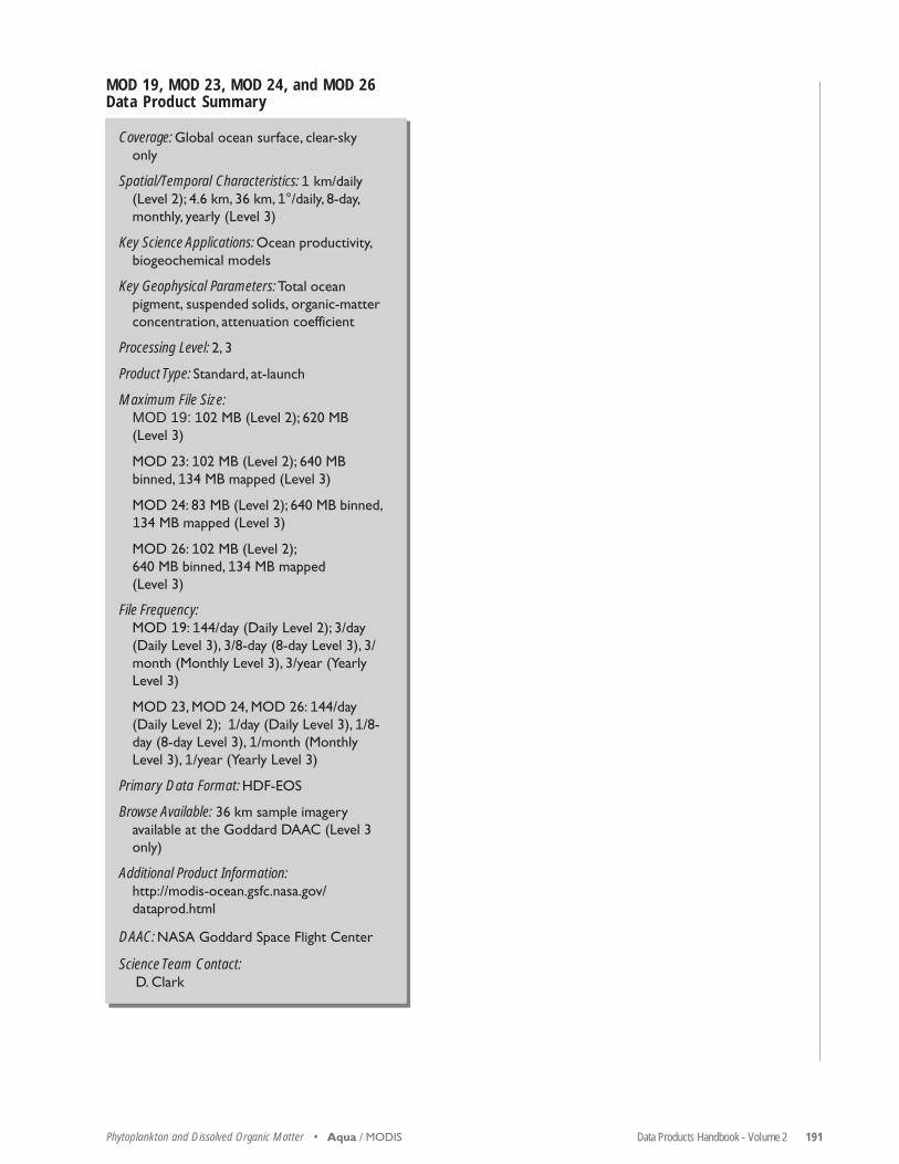
Data Products Handbook - Volume 2 191Phytoplankton and Dissolved Organic Matter •
MOD 19, MOD 23, MOD 24, and MOD 26Data Product Summary
Coverage: Global ocean surface, clear-skyonly
Spatial/Temporal Characteristics: 1 km/daily(Level 2); 4.6 km, 36 km, 1°/daily, 8-day,monthly, yearly (Level 3)
Key Science Applications: Ocean productivity,biogeochemical models
Key Geophysical Parameters: Total oceanpigment, suspended solids, organic-matterconcentration, attenuation coefficient
Processing Level: 2, 3
Product Type: Standard, at-launch
Maximum File Size:MOD 19: 102 MB (Level 2); 620 MB(Level 3)
MOD 23: 102 MB (Level 2); 640 MBbinned, 134 MB mapped (Level 3)
MOD 24: 83 MB (Level 2); 640 MB binned,134 MB mapped (Level 3)
MOD 26: 102 MB (Level 2);640 MB binned, 134 MB mapped(Level 3)
File Frequency:MOD 19: 144/day (Daily Level 2); 3/day(Daily Level 3), 3/8-day (8-day Level 3), 3/month (Monthly Level 3), 3/year (YearlyLevel 3)
MOD 23, MOD 24, MOD 26: 144/day(Daily Level 2); 1/day (Daily Level 3), 1/8-day (8-day Level 3), 1/month (MonthlyLevel 3), 1/year (Yearly Level 3)
Primary Data Format: HDF-EOS
Browse Available: 36 km sample imageryavailable at the Goddard DAAC (Level 3only)
Additional Product Information:http://modis-ocean.gsfc.nasa.gov/dataprod.html
DAAC: NASA Goddard Space Flight Center
Science Team Contact:D. Clark
Aqua / MODIS

192 Data Products Handbook - Volume 2 • Phytoplankton and Dissolved Organic Matter
U.S. East Coast Ocean-Color Image. This daily Coastal Zone Color Scanner (CZCS) product for the northeastern coast of the UnitedStates reveals the high pigment concentrations along the coast and the influence of the Gulf Stream. Phytoplankton concentrations,and additional ocean-carbon-system parameters from MODIS, will be considerably more accurate than was possible with the CZCSbecause of improvements in spectral bands, calibration, and algorithms. (From NASA GSFC.)
.1
.2
.4
.6
.81
10
PhytoplanktonPigment
Concentration(mg/m3)
Aqua / MODIS

Data Products Handbook - Volume 2 193Phytoplankton and Dissolved Organic Matter •
MODIS Chlorophyll Fluorescence(MOD 20)
Product Description
This Level 2 product contains several parametersdescribing ocean chlorophyll fluorescence properties.Fluorescence line height is a relative measure of theamount of radiance leaving the sea surface at the fluo-rescence wavelength of 683 nm. Fluorescence Effi-ciency provides a relative measure of the absorptionof PAR and its emission as chlorophyll fluorescence.The third parameter is Fluorescence Line Curvature.The spatial resolution will be 1 km for chlorophylllevels greater than 1.5 mg/m3 and 5 × 5 km for val-ues less than 1.5. The Level 2 product is produceddaily, and Level 3 is gridded and produced daily, 8-day weekly, monthly, and yearly.
Research and Applications
Solar-stimulated chlorophyll fluorescence is a mea-sure of the current photophysiology of phytoplank-ton, in contrast to the biomass estimate provided bychlorophyll. The product quantifies the level of pho-tosynthesis by phytoplankton in the ocean. Histori-cally, the coupling between fluorescence and chloro-phyll has been studied extensively, and recentresearch has focused on the use of Sun-stimulatedfluorescence to estimate primary productivity (Kieferand Reynolds, 1992). Basic fluorometric measure-ments are made using an instrument described byHolm-Hansen et al. (1965) that uses blue-light stimu-lation; this method has been used unchanged for 30years. Gower and Borstad (1990) was among the firstto attempt to use sun-stimulated radiance at 683 nmto estimate chlorophyll concentrations from aircraftand satellites.
Data Set Evolution
Inputs to the algorithm are chlorophyll concentration(within MOD 19), Absorbed Radiation by Phy-toplankton (ARP) (within MOD 22), and Water-Leav-ing Radiance (MOD 18). Water-leaving radiance forMODIS bands 13 (667 nm), 14 (678 nm), and 15(748 nm) are used in the algorithm. The algorithm isapplied to the daily input standard-product data setsand is remapped into standard Level 3 grids. The vali-dation approach will be to compare the fluorescenceresults with other MODIS data products (e.g., Chlo-rophyll a), with surface measurements, and with other
satellite-based estimates of the same products. Theproducts are produced only for non-cloud, glint-freeocean pixels during daylight hours.
Suggested Reading
Abbott, M.R. et al., 1982.
Abbott, M.R., and R.M. Letelier, 1998.
Chamberlin, W.S., and J. Marra, 1992.
Gower, F.J.R., and G.A. Borstad, 1990.
Holm-Hansen, O. et al., 1965.
Kiefer, D.A., and R.A. Reynolds, 1992.
Letelier, R.M. et al., 1997.
Topliss, B.J., and T. Platt, 1986.
MODIS Chlorophyll Fluorescence Summary
Coverage: Global ocean surface, clear-skyonly
Spatial/Temporal Characteristics: 1 km forchlorophyll levels greater than 2.0 mg/m3/daily, (Level 2); 4.6 km, 36 km, 1°/8-day,monthly, yearly (Level 3)
Key Science Applications: Ocean chlorophyll,ocean productivity
Key Geophysical Parameters: Chlorophyllfluorescence (fluorescence line height,fluorescence efficiency, fluorescence linecurvature)
Processing Level: 2, 3
Product Type: Standard, at-launch
Maximum File Size: 102 MB (Level 2); 640 MBbinned, 134 MB mapped (Level 3)
File Frequency: 144/day (Daily Level 2); 3/day(Daily Level 3), 3/week (Weekly Level 3),3/month (Monthly Level 3), 3/year (YearlyLevel 3)
Primary Data Format: HDF-EOS
Additional Product Information:http://modis-ocean.gsfc.nasa.gov/dataprod.html
DAAC: NASA Goddard Space Flight Center
Science Team Contact:M. Abbott
Aqua / MODIS

194 Data Products Handbook - Volume 2 • Phytoplankton and Dissolved Organic MatterAqua / MODIS
Chlorophyll a Concentrations (MOD 21) as measured by MO-DIS in the Indian Ocean on March 1, 2000. Chlorophyll, the greenpigment in plants and phytoplankton, absorbs sunlight for usein photosynthesis. Note the high concentrations (light grays) inthe Arabian Sea and relatively low concentrations (dark grays)in the Bay of Bengal. The black color in the image representsland areas and gaps between successive satellite orbits, and thegray “stripes” indicate where clouds or sun glint prevented ac-curate measurements.
Chlorophyll a (Chl)
Chlorophyll Fluorescence (MOD 20) as measured from the TerraMODIS instrument on March 1, 2000. Phytoplankton re-emitsome of the light that is captured by chlorophyll as fluorescence.The amount of fluorescence is roughly proportional to the amountof chlorophyll, so in this image, for example, high fluorescencecan be found in the Arabian Sea.
Fluorescence Line Height (FLH)
Ratio of Chlorophyll Fluorescence (MOD 20) to Chlorophyll aConcentration (MOD 21), illustrating the considerable variabil-ity in the amount of fluorescence per unit of chlorophyll. Thisvariability is largely a function of the health of the phytoplank-ton. A high ratio implies lower growth rates, as the light cap-tured by phytoplankton is being re-emitted as fluorescence ratherthan being used for photosynthesis. Phytoplankton in the Ara-bian Sea are probably growing more rapidly than elsewhere, per-haps in response to dust inputs (which are rich in iron) from theArabian Peninsula.
FLH/Chl Ratio
(MODIS Chlorophyll Fluorescence, continued)

Data Products Handbook - Volume 2 195Phytoplankton and Dissolved Organic Matter • Aqua / MODIS
MODIS Chlorophyll a PigmentConcentration (MOD 21) andAbsorption Coefficients(MOD 36)
Product Description
This is a Level 2 and 3 product which contains oceanchlorophyll a pigment concentration for Case 1 andCase 2 waters at 1-km resolution. It is produced dailyat Level 2 and daily, 8-day weekly, monthly, andyearly at Level 3. Absorption parameters generatedby the chlorophyll algorithm are also provided as theintermediate product MOD 36, Absorption Coeffi-cients, which includes absorption due to water, phy-toplankton, detritus, and gelbstoff, and gelbstoff ab-sorption only. Valid data exist only for oceancloud-free pixels and the weekly composite will bean average of cloud-free acquisitions for each oceanpixel.
Research and Applications
Chlorophyll a concentration is a key input to theOcean Primary Productivity product (MOD 27) andis used to trace oceanographic currents, jets, andplumes. The product provides the concentration ofchlorophyll in Case 1 sea water (water that has opti-cal properties that are dominated by chlorophyll andassociated covarying detrital pigments) and in Case2 waters (waters that contain substances that affectoptical properties but do not covary with chlorophyll,such as gelbstoff (marine chromomorphic dissolvedorganic matter [CDOM] substance that absorbs at 400nm), suspended sediments, coccolithophores, detri-tus, and bacteria). The algorithm derives from exten-sive research using CZCS data in which good per-formance was obtained for Case 1 waters and hasevolved to perform successfully for the Case 2 wa-ters for the MODIS algorithm. The 1-km resolutionand nearly daily coverage will allow the observationof mesoscale oceanographic features in coastal andestuarine environments, which are of increasing im-portance in marine science studies.
Data Set Evolution
The product algorithm is based on a semi-analytical,bio-optical model of remote sensing reflectancewhich uses Water-Leaving Radiance (MOD 18), PAR(MOD 22), and Absorption Coefficients (MOD 36).
The model is inverted to obtain the absorption coef-ficient due to phytoplankton at 675 nm, and chloro-phyll a concentration is derived from this coefficient.The algorithm will be thoroughly tested during theSeaWiFS project, and post-launch validation will beconducted using data from instrumented collectioncruises through ocean test sites including the nineused for algorithm development. Also, hyperspectraldata will be used to simulate the 10-nm bands andproduce comparison results.
Suggested Reading
Austin, R.W., 1974.
Carder, K.L. et al., 1986.
Carder, K.L. et al., 1991a,b.
Holm-Hansen, O., and B. Riemann, 1978.
Lee, Z.P. et al., 1996.
Smith, R.C., and K.S. Baker, 1982.

196 Data Products Handbook - Volume 2 • Phytoplankton and Dissolved Organic MatterAqua / MODIS
(MODIS Chlorophyll a Pigment Concentration and AbsorptionCoefficients, continued)
MODIS Chlorophyll a Pigment Concentrationand Absorption Coefficients Summary
Coverage: Global ocean surface, clear-skyonly
Spatial/Temporal Characteristics: 1 km/daily(Level 2); 4.6 km, 36 km, 1°/daily, 8-day,monthly, yearly (Level 3)
Key Science Applications: Ocean productivity,bio-optical properties
Key Geophysical Parameters: Case 1 and 2chlorophyll a concentration, absorptioncoefficients
Processing Level: 2, 3
Product Type: Standard, at-launch
Maximum File Size:MOD 21: 83 MB (Level 2); 640 MB binned,134 MB mapped (Level 3)
MOD 36: 102 MB (Level 2); 865 MBbinned, 134 MB mapped (Level 3)
File Frequency: 144/day (Daily Level 2); 2/day(Daily Level 3), 2/8-day (8-day Level 3), 2/month (Monthly Level 3), 2/year (YearlyLevel 3)
Primary Data Format: HDF-EOS
Browse Available: 36 km sample imageryavailable at the Goddard DAAC (Level 3only)
Additional Product Information:http://modis-ocean.gsfc.nasa.gov/dataprod.html
DAAC: NASA Goddard Space Flight Center
Science Team Contact:K. Carder
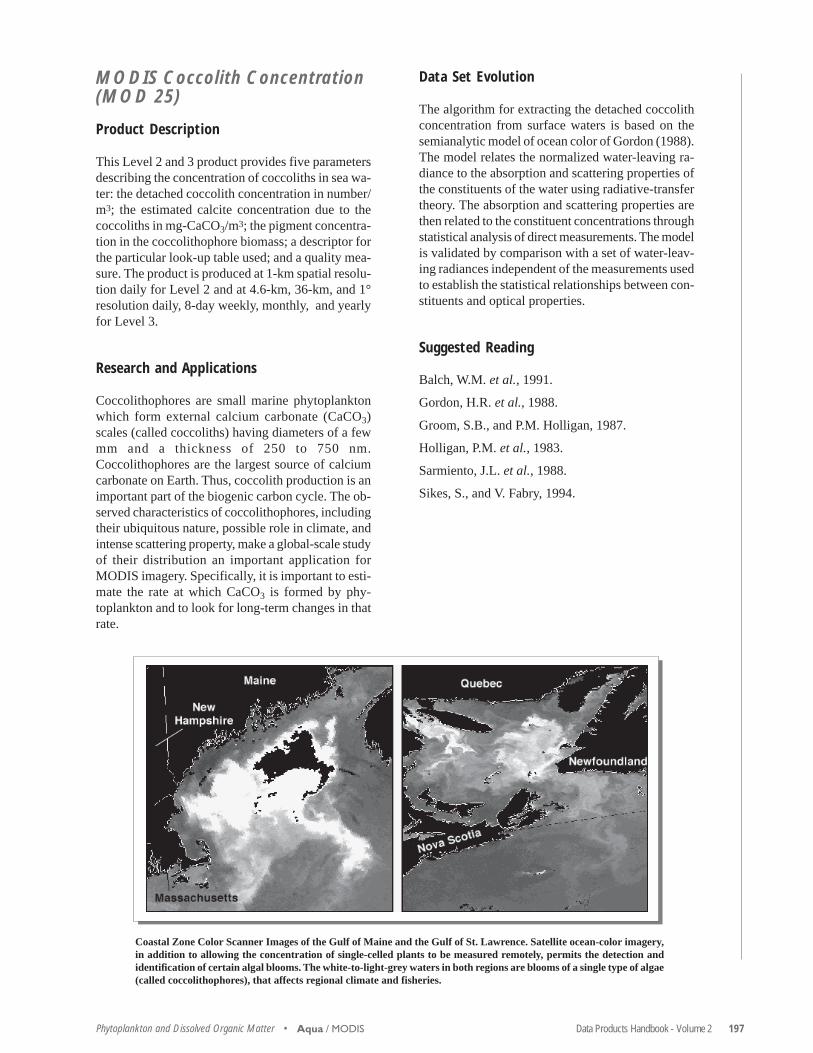
Data Products Handbook - Volume 2 197Phytoplankton and Dissolved Organic Matter • Aqua / MODIS
Coastal Zone Color Scanner Images of the Gulf of Maine and the Gulf of St. Lawrence. Satellite ocean-color imagery,in addition to allowing the concentration of single-celled plants to be measured remotely, permits the detection andidentification of certain algal blooms. The white-to-light-grey waters in both regions are blooms of a single type of algae(called coccolithophores), that affects regional climate and fisheries.
MODIS Coccolith Concentration(MOD 25)
Product Description
This Level 2 and 3 product provides five parametersdescribing the concentration of coccoliths in sea wa-ter: the detached coccolith concentration in number/m3; the estimated calcite concentration due to thecoccoliths in mg-CaCO3/m3; the pigment concentra-tion in the coccolithophore biomass; a descriptor forthe particular look-up table used; and a quality mea-sure. The product is produced at 1-km spatial resolu-tion daily for Level 2 and at 4.6-km, 36-km, and 1°resolution daily, 8-day weekly, monthly, and yearlyfor Level 3.
Research and Applications
Coccolithophores are small marine phytoplanktonwhich form external calcium carbonate (CaCO3)scales (called coccoliths) having diameters of a fewmm and a thickness of 250 to 750 nm.Coccolithophores are the largest source of calciumcarbonate on Earth. Thus, coccolith production is animportant part of the biogenic carbon cycle. The ob-served characteristics of coccolithophores, includingtheir ubiquitous nature, possible role in climate, andintense scattering property, make a global-scale studyof their distribution an important application forMODIS imagery. Specifically, it is important to esti-mate the rate at which CaCO3 is formed by phy-toplankton and to look for long-term changes in thatrate.
Data Set Evolution
The algorithm for extracting the detached coccolithconcentration from surface waters is based on thesemianalytic model of ocean color of Gordon (1988).The model relates the normalized water-leaving ra-diance to the absorption and scattering properties ofthe constituents of the water using radiative-transfertheory. The absorption and scattering properties arethen related to the constituent concentrations throughstatistical analysis of direct measurements. The modelis validated by comparison with a set of water-leav-ing radiances independent of the measurements usedto establish the statistical relationships between con-stituents and optical properties.
Suggested Reading
Balch, W.M. et al., 1991.
Gordon, H.R. et al., 1988.
Groom, S.B., and P.M. Holligan, 1987.
Holligan, P.M. et al., 1983.
Sarmiento, J.L. et al., 1988.
Sikes, S., and V. Fabry, 1994.

198 Data Products Handbook - Volume 2 • Phytoplankton and Dissolved Organic MatterAqua / MODIS
MODIS Ocean PrimaryProductivity (MOD 27)
Product Description
This Level 4 product provides an estimate of theOcean Primary Productivity on an 8-day and an an-nual basis at spatial resolutions of 4.6 km and 36 km.
Research and Applications
The objective of the product is to quantify the mag-nitude and interannual variability (for decadal trends)in the oceanic primary productivity and phytoplank-ton carbon fixation. Primary productivity is the timerate of change of phytoplankton biomass, and, withallowance for excreted soluble carbon compounds,reflects the daily integrated photosynthesis within thewater column. The integral of the values over the yearis the annual primary productivity. The annual pro-ductivity product will be used for global- and re-gional-scale studies of interannual variability of oceanproductivity, for comparisons with annual summa-tions of short-term analytic estimates, and for com-parison with global biogeochemical models.
Data Set Evolution
Ocean primary-productivity algorithms fall into twogeneral classes, termed empirical and analytic algo-rithms. The empirical approach is based on simplecorrelation between time-averaged in situ estimatesof productivity and satellite-derived estimates of sur-face chlorophyll concentration. The analytic approachis based on models of the general photosynthetic re-sponse of the algal biomass as a function of majorenvironmental variables such as light, temperature,and nutrient concentration. The overall methodolo-gies differ significantly in the way various param-eters are estimated and in the way they are assignedspatially and temporally across ocean basins. Theapproach taken for the MODIS algorithm is to beginimplementation of an annual, global, empirical algo-rithm for at-launch product generation, while pursu-ing a vigorous research program within the SeaWiFSScience Team, to develop a consensus analytic algo-rithm for short-term (daily to weekly) global produc-tivity. Cloudiness prevents deriving chlorophyll aconcentrations over about 60% of the ocean on dailybasis, excluding that already lost due to high sun glint.Chlorophyll a concentrations derived from all avail-able sensors, including the Terra and Aqua MODISinstruments, will be used to increase sampling fre-
(MODIS Coccolith Concentration, continued)
MODIS Coccolith Concentration Summary
Coverage: Global ocean surface, clear-sky only
Spatial/Temporal Characteristics: 1 km/daily(Level 2); 4.6 km, 36 km, 1°/daily, 8-day,monthly, yearly (Level 3)
Key Science Applications: Input to global bio-geochemical cycle models
Key Geophysical Parameters: Coccolith and cal-cite concentration, pigment concentrationin coccolithophore blooms
Processing Level: 2, 3
Product Type: Standard, at-launch
Maximum File Size: 102 MB (Level 2);640 MB binned, 134 MB mapped(Level 3)
File Frequency: 144/day (Daily Level 2); 3/day(Daily Level 3), 3/8-day (8-day Level 3),3/month (Monthly Level 3), 3/year (YearlyLevel 3)
Primary Data Format: HDF-EOS
Browse Available: 36 km sample imageryavailable at the Goddard DAAC (Level 3only)
Additional Product Information:http://modis-ocean.gsfc.nasa.gov/dataprod.html
DAAC: NASA Goddard Space Flight Center
Science Team Contacts:H.R. GordonW.B. Balch
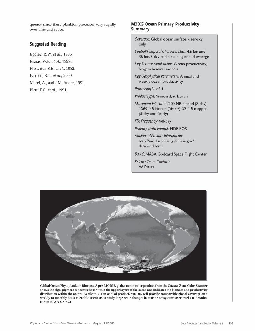
Data Products Handbook - Volume 2 199Phytoplankton and Dissolved Organic Matter • Aqua / MODIS
Global Ocean Phytoplankton Biomass. A pre-MODIS, global ocean-color product from the Coastal Zone Color Scannershows the algal pigment concentrations within the upper layers of the ocean and indicates the biomass and productivitydistribution within the oceans. While this is an annual product, MODIS will provide comparable global coverage on aweekly-to-monthly basis to enable scientists to study large-scale changes in marine ecosystems over weeks to decades.(From NASA GSFC.)
quency since these plankton processes vary rapidlyover time and space.
Suggested Reading
Eppley, R.W. et al., 1985.
Esaias, W.E. et al., 1999.
Fitzwater, S.E. et al., 1982.
Iverson, R.L. et al., 2000.
Morel, A., and J.M. Andre, 1991.
Platt, T.C. et al., 1991.
MODIS Ocean Primary ProductivitySummary
Coverage: Global ocean surface, clear-skyonly
Spatial/Temporal Characteristics: 4.6 km and36 km/8-day and a running annual average
Key Science Applications: Ocean productivity,biogeochemical models
Key Geophysical Parameters: Annual andweekly ocean productivity
Processing Level: 4
Product Type: Standard, at-launch
Maximum File Size: 1200 MB binned (8-day),1360 MB binned (Yearly); 32 MB mapped(8-day and Yearly)
File Frequency: 4/8-day
Primary Data Format: HDF-EOS
Additional Product Information:http://modis-ocean.gsfc.nasa.gov/dataprod.html
DAAC: NASA Goddard Space Flight Center
Science Team Contact:W. Esaias

200 Data Products Handbook - Volume 2 • Phytoplankton and Dissolved Organic MatterAqua / MODIS
MODIS PhycoerythrinConcentration (MOD 31)
Product Description
This product consists of three parameters which givethe concentration of one of the major algal pigmentgroups in ocean water, Phycoerythrin. The three pa-rameters are Phycoerythrobilin Concentration,Phycourobilin Concentration, and Constituent Inher-ent Optical Properties (CDOM absorption, chloro-phyllous absorption, and particulate backscatter).These quantities are provided for Level 2 at 1-kmspatial resolution daily and for Level 3 daily, 8-dayweekly, monthly, and yearly at 4.6-km, 36-km, and1° resolution. The product is valid only for clear-skyocean pixels.
Phycoerythrin is one of three major algal pigmentgroups found in marine phytoplankton and bacteria(Bidigare, 1990). The phycoerythrins are further sub-divided into phycourobilin-rich (PUB) andphycoerythrobilin-rich (PEB) phycoerythrins. Thisalgorithm retrieves both PUB- and PEB- rich cases.Phycoerythrin is a chlorophyll accessory pigment andserves to receive photosynthetically usable light inthe 480-505-nm and 540-560-nm ranges. It is usedto infer the global extent of phycoerythrin-bearingphytoplankton such as cyanobacteria, which are ni-trogen-fixing and thus provide information on thenitrogen cycle. Used in conjunction with phytoplank-ton chlorophyllous pigment, the apparent species di-versity of the oceans can be inferred.
Research and Applications
One of the intended uses of the phycoerythrin dataproduct is to allow scientific investigators to studythe global distributions of the phycoerythrin pigmentand, in so doing, to allow definition of the diversityof phycoerythrin-bearing species such ascyanobacteria. When used in conjunction with chlo-rophyll distribution, phycoerythrin determination al-lows global phytoplankton species variability stud-ies.
Data Set Evolution
The phycoerythrin retrieval algorithm requires wa-ter-leaving radiances generated from the incidentsolar irradiance, the total backscatter, and the totalabsorption of sea water. The PUB and PEB param-
eters are retrieved by a sequential-convergent-itera-tion method (Gordon et al., 1988) that uses five in-dependent bands. MODIS band 10 (488 nm) and band12 (551 nm) correspond to the peaks of the PUB andPEB phycoerythrins. The major assumption for thealgorithm is that the pigment-specific absorption-co-efficient spectral model used is applicable for the oce-anic province where the satellite image was acquired.The algorithm will be validated by ship and airbornelaser-induced and water Raman-normalized fluores-cence measurements.
Suggested Reading
Bidigare, R.R. et al., 1990.
Culver, M.E., and M.J. Perry, 1994.
Gordon, H.R. et al., 1988.
Hoge, F.E., and R.N. Swift, 1986.
Hoge, F.E., and R.N. Swift, 1990.
Hoge, F.E. et al., 1999a.
Hoge, F.E. et al., 1999b.

Data Products Handbook - Volume 2 201Phytoplankton and Dissolved Organic Matter •
MODIS Phycoerythrin ConcentrationSummary
Coverage: Global ocean surface, clear-skyonly
Spatial/Temporal Characteristics: 1 km/daily(Level 2); 4.6 km, 36 km, 1°/daily, 8-day,monthly, yearly (Level 3)
Key Science Applications: Global phytoplank-ton species studies, ocean productivitymodels
Key Geophysical Parameters:Phycoerythrobilin-rich (PEB) andphycourobulin-rich (PUB) phycoerythrins
Processing Level: 2, 3
Product Type: Research, at-launch
Maximum File Size: 102 MB (Level 2); 640 MBbinned, 134 MB mapped (Level 3)
File Frequency: 144/day (Daily Level 2); 2/day(Daily Level 3), 2/8-day (8-day Level 3),2/month (Monthly Level 3), 2/year (YearlyLevel 3)
Primary Data Format: HDF-EOS
Browse Available: 36 km sample imageryavailable at the Goddard DAAC (Level 3only)
Additional Product Information:http://modis-ocean.gsfc.nasa.gov/dataprod.html
DAAC: NASA Goddard Space Flight Center
Science Team Contact:F.E. Hoge
Aqua / MODIS

203
Snow and Ice CoverAqua
• AMSR-E• MODIS

204 Data Products Handbook - Volume 2 • Snow and Ice Cover
Snow and Ice Cover – AnOverview
Relationship to Global Change Issues
Snow and ice cover dramatically influence surfacealbedo, hydrologic properties, the interactions be-tween the atmosphere and the underlying surface, andregulation of ecosystem biological activity. For in-stance, when sea ice is formed in the ocean or snowis deposited on land, these processes can double thedegree to which the surface reflects incoming solarenergy, hence affecting the Earth’s radiation balanceand, in turn, its climate. Furthermore, both snow andice are highly variable components of the climatesystem, changing dramatically from summer to win-ter, and, to a lesser extent, from year to year. Thecombination of high variability and impacts on criti-cal climate processes insures the importance of moni-toring snow and ice to the understanding of globalchange.
Two key sensors on board Aqua that will provideenhanced global sea ice and snow measurements tosupplement existing data sets are the AMSR-E andMODIS. Both will provide information to be used inthe development of more accurate models to help un-derstand and predict Earth’s climate and the role ofsnow and ice in it.
AMSR-E data will provide daily, global coverageof sea ice and snow regardless of cloud conditions ordarkness. The derived sea ice and snow parameterswill be used both operationally and for climate re-search. By extending the existing time series of seaice and snow parameters, which currently span over20 years, scientists expect to obtain a better under-standing of global, hemispheric, and regional vari-abilities on seasonal, interannual, and decadal timescales. The improved spatial resolution possible fromthe AMSR-E sensor, relative to previous satellitepassive-microwave instruments, will also allowgreater insight into the processes which define therole of the cryosphere in the climate system.
MODIS data will be used to monitor the dynamicsof large-area (greater than 10 square kilometers) snowand ice cover using daily and 8-day products. Infor-mation about snow and ice cover, including surfacetemperature, is important for a number of agricul-tural, industrial, social, and environmental reasons.For example, in some regions snow cover data canbe critical in successfully predicting water supply,planning for agricultural and industrial developments,anticipating flooding, forecasting crop yield, and es-timating freeze damage.
Overview
Product Overview
Global snow-water equivalent and snow depth willbe mapped daily and every five days over the Earth’sland surfaces at 25-km resolution using the AMSR-Esnow-water equivalent and snow-depth algorithm. Aglobal, daily snow-storage map will be an at-launchAMSR-E product. Snow-water equivalent values willbe inferred based on the resampled brightness data.After one day, a daily map will be generated bycompositing all the data within that day. The MO-DIS snow cover product will be mapped daily and as8-day composites at 500-m resolution over the Earth’sland surfaces, using an algorithm based on the nor-malized difference of a visible and a shortwave-in-frared band.
The sea ice products derived from AMSR-E in-clude sea ice concentration, ice temperature, and snowdepth over sea ice. Daily sea ice concentrations andice temperatures will be mapped on the standardSSM/I grid. Ascending data will also be separatedfrom descending data for day/night discrimination.Sea ice concentrations will be mapped at both 25-km and 12.5-km resolutions while sea ice tempera-tures will be mapped on the 25-km-resolution gridonly. Snow depth on sea ice will be a five-day prod-uct and mapped at a grid resolution of 12.5 km. Adaily sea ice product will also be obtained fromMODIS at a much finer, 1 km, resolution than theAMSR-E product but with use limited largely tocloud-free conditions. The MODIS sea ice productis based on the normalized difference between a vis-ible and a shortwave-infrared band signal.
Product Interdependency and Continuitywith Heritage Data
There have been several satellite missions that havecollected snow and ice data for many years. Snowand ice are among the variables included in NASA’sPathfinder Program, which is providing research-quality data sets on global change from past and cur-rent satellite instruments. The heritage of both theAMSR-E and MODIS sensors is strong. Data setsfrom these sensors will extend those from historicaland current sensors and provide the continuity neededfor long-term global climate-change studies.
The first detailed data sets of sea ice distributionsregardless of cloud cover or solar illumination camefrom the data of the Electrically Scanning MicrowaveRadiometer (ESMR) on the Nimbus 5 satellitelaunched in December 1972. ESMR and its succes-sor, the Scanning Multichannel Microwave Radiom-

Data Products Handbook - Volume 2 205Snow and Ice Cover •
eter (SMMR), launched on Nimbus 7 in October1978, provided the data for three major sea ice at-lases describing the seasonal cycles and interannualvariability of the Arctic and Antarctic sea ice coversfor the years 1973-76 and 1978-87. The SMMR hasbeen superseded by the Special Sensor Microwave/Imager (SSM/I), which has flown as part of the De-fense Meteorological Satellite Program (DMSP)since 1987. The SSM/I is similar to SMMR, and itsdata also have been analyzed to determine snow coverand sea ice conditions. Most recently, time-seriesanalyses of the combined SMMR and SSM/I datasets have yielded information on global sea ice trendsand on regional and hemispheric variabilities span-ning a 20-year period. The AMSR-E data will helpto extend this 20-year sea ice record.
Other sources of historical satellite data for ice andsnow are Landsat, which started operation (as theEarth Resources Technology Satellite) in 1972, theAdvanced Very High Resolution Radiometer(AVHRR) on the NOAA satellites, which started op-eration in 1978, Seasat, Geosat, and many Japanese,European, and Russian satellite sensors. Landsat pro-vides very high resolution (15-80 m in the visibleand near-infrared bands, and 60-120 m in the ther-mal-infrared bands), while AVHRR provides moder-ate resolution (1 km) in the visible and infrared chan-nels. Because of higher spatial resolution, broaderspectral range, and extensive calibration and valida-tion programs, both AMSR-E and MODIS are ex-pected to provide more accurate data products thanis currently possible with their primary precursors,the SSM/I and AVHRR, respectively.
Suggested Reading
Chang, A.T.C. et al., 1987.
Chang, A.T.C. et al., 1997.
Comiso, J.C. et al., 1997.
Comiso, J.C., 2000.
Foster, J.L. et al., 1984.
Gloersen, P. et al., 1992.
Hall, D.K. et al., 1995.
Klein, A.G. et al., 1998.
Markus, T., and D.J. Cavalieri, 1998.
Markus, T., and D.J. Cavalieri, 2000.
Parkinson, C.L., 1997.
Parkinson, C.L. et al., 1987.
Weeks, W.F., 1981.
Zwally, H.J. et al., 1983.
Overview

206 Data Products Handbook - Volume 2 • Snow and Ice Cover
Landsat TM Scene of Northern Montana including Glacier National Park, after the application of the SNOMAP algorithm(Hall et al., 1995). The TM Scene was acquired on March 14, 1991 (scene i.d. #5256917454). (Note: Snow and non-snow featureswere classified automatically by the SNOMAP algorithm, but cloud features were classified by supervised classification.)
SNOW CLOUDS OTHER
Overview
Data Products Handbook - Volume 2 207Snow and Ice Cover •
AMSR-E Sea Ice Concentration
Product Description
Sea ice concentrations will be produced from modi-fied versions of the NASA Team algorithm (Markusand Cavalieri, 2000) and the Bootstrap algorithm(Comiso and Zwally, 1997). The NASA Team algo-rithm will be used as the standard algorithm to pro-cess Arctic data, while the Bootstrap algorithm willbe used as the standard algorithm to process Antarc-tic data. Ice-concentration-difference maps derivedfrom the two algorithms for both hemispheres willalso be archived for comparison. Sea ice concentra-tions from both algorithms and their differences willbe produced as gridded products (Level 3) andmapped onto a 25-km grid, enabling ready continua-tion of a twenty-year historical data set derived fromSMMR and SSM/I. The ice-concentration productswill also be gridded at 12.5 km to take advantage ofthe higher spatial resolution of the sensor. The gridsat both resolutions use a polar stereographic projec-tion defined for the SMMR and SSM/I data sets(NSIDC, 1996).
Research and Applications
Polar sea ice is an important component of the glo-bal climate system. It insulates the atmosphere fromthe oceanic heat below in winter and keeps the oceanfrom absorbing heat from the sun in the spring andsummer. Because of the high albedo of sea ice andits snow cover, it also plays an important role in theregional and global energy balance. The most impor-tant measure of the polar sea ice cover is itsconcentration. This product enables quantification ofice-free water in the leads and polynyas within theice pack as well as the extent of the sea ice coveritself. Over twenty years of satellite passive-micro-wave sea ice data exist and have been used to studyseasonal, regional, and interannual sea ice variabili-ties of the Arctic and Antarctic (e.g., Gloersen etal., 1992; Jacobs and Comiso, 1997; Cavalieri et al.,1997).
Data Set Evolution
The modified NASA Team and Bootstrap sea ice al-gorithms have considerable heritage. The NASATeam algorithm is based on the use of radiance ra-tios called the polarization and the spectral gradientratio. The technique has been used since the launchof the Nimbus 7 SMMR in 1978 (Cavalieri et al.,
1984; Gloersen and Cavalieri, 1986) and continuedwith modifications (Cavalieri et al., 1991) with theseries of SSM/I sensors first launched in 1987. TheBootstrap algorithm makes use of the multifrequencycapabilities of the sensor to reduce errors due to varia-tions in emissivity and temperature, and, like theNASA Team algorithm, has been applied to both theSMMR and SSM/I data sets (Comiso, 1986; Comiso,1995). The theoretical foundation and details of thetwo original algorithms and a comparative analysisof results from a year of SSM/I data are presented inComiso et al. (1997).
Suggested Reading
Cavalieri, D.J. et al., 1984.
Cavalieri, D.J. et al., 1991.
Cavalieri, D.J. et al., 1997.
Comiso, J.C., 1986.
Comiso, J.C., 1995.
Comiso, J.C., and H.J. Zwally, 1997.
Comiso, J.C. et al., 1997.
Gloersen P., and D.J. Cavalieri, 1986.
Gloersen, P. et al., 1992.
Jacobs, S.S., and J.C. Comiso, 1997.
Markus, T., and D.J. Cavalieri, 2000.
NSIDC, 1996.
Aqua / AMSR-E

208 Data Products Handbook - Volume 2 • Snow and Ice Cover
AMSR-E Snow Depth on Sea Ice
Product Description
Snow depth on sea ice will be mapped every fivedays at a 12.5-km grid resolution. The algorithm, de-scribed in detail by Markus and Cavalieri (1998),makes use of the spectral-gradient ratio, defined us-ing the 18- and 37-GHz vertically polarized radiances,and the total sea ice concentration measured with themodified NASA Team sea ice algorithm (Markus andCavalieri, 2000). Currently, the algorithm is limitedto the Southern Ocean and to the Arctic seasonal seaice zones. Snow depth is measured in centimeterswith a precision of 1 cm and an estimated accuracyof 5 cm.
Research and Applications
The overall importance of snow depth on sea ice tothe climate system is well documented (e.g., Ledley,1991; Eicken et al., 1995). Snow cover on sea iceprimarily affects the climate through its effect onsurface albedo and the thermal insulation betweenocean and atmosphere. Given that the change in seaice coverage from summer to winter is over 15 mil-lion km2 in the Southern Ocean and 5 million km2 inthe Arctic, the effect of snow cover can besubstantial. Snow depth and accumulation rate areimportant variables in the fresh-water budget of thepolar oceans. A quantitative knowledge of snow-depth variability could provide a useful estimate ofprecipitation minus evaporation (P-E), which is criti-cally needed in state-of-the-art coupled ice-oceanmodels (Häkkinen, 1995). Current applications of theretrieved snow depths over the Southern Ocean in-clude the study of interannual and regional variabili-ties of snow depth on sea ice (Markus and Cavalieri,1998) and a study of mixed-layer ocean propertiesusing an ECMWF-SSM/I forced mixed-layer model(Markus, 1999).
Data Set Evolution
The snow-depth-on-sea-ice algorithm has consider-able heritage in Nimbus 7 SMMR and the DMSPSSM/I snow-depth algorithms derived for land ap-plications (e.g., Chang et al., 1987). The instrumentchannels used are similar (18/19 GHz and 37 GHz),but the functional form is different, making use ofratios of radiances in the snow-depth-on-sea-ice al-gorithm instead of linear differences for the land al-gorithm. In contrast to the Equal-Area Scalable Earth
AMSR-E Sea Ice Concentration Summary
Coverage: Global
Spatial/Temporal Characteristics: 12.5 km and25 km/ascending, descending, and dailyaverages
Key Geophysical Parameters: Sea ice concen-tration and difference
Processing Level: 3
Product Type: Standard, at-launch
Maximum File Size: 53 MB
File Frequency: 1/day
Primary Data Format: HDF-EOS
Browse Available: Accompanies data product
Additional Product Information:http://wwwghcc.msfc.nasa.gov/AMSR/html/amsr_products.html
DAAC: National Snow and Ice Data Center
Science Team Contacts:D. J. CavalieriJ. C. Comiso
(AMSR-E Sea Ice Concentration, continued)
Aqua / AMSR-E

Data Products Handbook - Volume 2 209Snow and Ice Cover • Aqua / AMSR-E
(EASE) grid used for snow cover on land, the Level3 grid used for snow depth on sea ice will be the so-called SSM/I polar stereographic grid, from NSIDC,with a grid size of 12.5 km. It matches the 12.5-kmgrid used for sea ice concentration.
Suggested Reading
Chang, A.T.C. et al., 1997.
Eicken, H. et al., 1995.
Häkkinen, S., 1995.
Ledley, T.S., 1991.
Markus, T., and D.J. Cavalieri, 1998.
Markus, T., and D.J. Cavalieri, 2000.
Markus, T., 1999.
NSIDC, 1996.
AMSR-E Snow Depth on Sea Ice Summary
Coverage: Southern Ocean and the Arcticseasonal sea ice zones
Spatial/Temporal Characteristics: 12.5 km/5-day average
Key Geophysical Parameters: Snow depth onsea ice
Processing Level: 3
Product Type: Standard, at-launch
Maximum File Size: 53 MB
File Frequency: 1/day
Primary Data Format: HDF-EOS
Browse Available: Accompanies data product
Additional Product Information:http://wwwghcc.msfc.nasa.gov/AMSR/html/amsr_products.html
DAAC: National Snow and Ice Data Center
Science Team Contacts:D. J. CavalieriJ. C. Comiso
AMSR-E Sea Ice Temperatures
Product Description
Sea ice temperatures will be produced from a modi-fied version of the Bootstrap algorithm and from asimple relationship among ice temperature, ice emis-sivity, and ice concentration. Sea ice temperatureswill be produced as gridded products (Level 3) andmapped onto a 25-km grid defined for the SMMRand SSM/I data sets by NSIDC. It is based on a polarstereographic projection.
Research and Applications
Satellite data provide a quantification of the polarsea ice cover in only two dimensions. Thickness, thethird dimension, is not currently observable with sat-ellite systems. While changes in ice temperature areclosely linked with the temperatures of the ocean andatmosphere, these changes may also reflect changesin ice thickness and snow cover. For example, awarming of the mixed layer of the Arctic Ocean maylead to a thinning of the ice cover, which in turn mayresult in a warming of the ice. Thus, by monitoringthe ice temperature, the snow depth, and the surfacetemperature derived, for example, from MODIS andAVHRR data (e.g., Comiso, 1999), it may be pos-sible to detect changes in ice thickness.
Data Set Evolution
Microwave observations of sea ice at 6 GHz repre-sent emissions primarily from the snow/ice interfaceand below. Since the emissivity for sea ice is rela-tively stable at this frequency, SMMR data have beenused by Gloersen et al. (1992) to obtain maps of icetemperatures from 1979 through 1987. This time se-ries was discontinued in 1987 because the lowest fre-quency for SSM/I is 19 GHz, which is not suitablefor the purpose. The AMSR-E will have a 6-GHzchannel and will provide the opportunity to obtainsea ice temperatures once again. The AMSR-E algo-rithm for ice temperature will be part of the revisedBootstrap Algorithm (Comiso and Zwally, 1997) thatmakes use of 6-GHz information to reduce spatialvariations in ice temperatures. The algorithm is dif-ferent from that of Gloersen et al. in that the initialice concentration used to calculate the effective emis-sivity at 6 GHz is derived from a combination of the6- and 37-GHz data, using the Bootstraptechnique. Also, a threshold of 80% ice concentra-

210 Data Products Handbook - Volume 2 • Snow and Ice Cover
AMSR-E Snow-Water Equivalentand Snow Depth
Product Description
Snow-water equivalent (SWE) and snow depth willbe mapped daily and every five days over the Earth’sland surfaces at 25-km resolution using an AMSR-Esnow-water-equivalent and snow-depth algorithm. Aglobal, daily snow-storage map will be an at-launchAMSR-E product. Snow-water-equivalent values willbe inferred, based on the resampled brightness data.After one day, a daily map will be generated bycompositing all the data within one day.
Snow storage is a key parameter of the global en-ergy and water balance. Snow-water-equivalent val-ues for the U.S. are currently mapped by NOAA/NWS/NOHRSC based on gamma radiation data. AnNOHRSC low-flying aircraft collects data over se-lected flight lines a couple of times per year duringthe winter season. Snow-water-equivalent valuesbetween the flight lines are generated by optimuminterpolation. Qualities of these data are difficult toassess.
Research and Applications
The objective of this product is to quantify the amountand interannual variability of snow storage duringthe winter season. Snow is one of the most importantrenewable resources, for instance providing over 70%of the water supply in the western U.S. Informationon the amount of snow storage and timing of dis-charge is critical for resource managers. Untimelymelting of the snowpack could cause enormous dam-age to properties and loss of human lives.
Data Set Evolution
The algorithm to retrieve the snow-water equivalentfrom AMSR-E data has a considerable heritage. It isbased on the observations from multi-frequency ra-diometers. The current algorithm is built on the al-gorithm developed for the SMMR data. Due to theeffects of grain size, density, stratigraphy, and wet-ness on microwave signals, a statistical retrieval ap-proach has been adopted.
Global snow cover will be mapped using a visiblesensor at a resolution of 500 m (MOD 10). Thesedata could provide snow mapping at basin scale forhydrological model applications. The persistent cloud
tion used by Gloersen et al., below which the tem-perature is set to 271 K, is not used.
Suggesting Reading
Comiso, J.C., 2000.
Comiso, J.C., and H.J. Zwally, 1997.
Gloersen, P. et al., 1992.
NSIDC, 1996.
AMSR-E Sea Ice Temperatures Summary
Coverage: Global
Spatial/Temporal Characteristics: 25 km/ascend-ing, descending, and daily averages
Key Geophysical Parameters: Sea ice tempera-ture
Processing Level: 3
Product Type: Standard, at-launch
Maximum File Size: 19.5 MB
File Frequency: 1/day
Primary Data Format: HDF-EOS
Browse Available: Accompanies data product
Additional Product Information:http://wwwghcc.msfc.nasa.gov/AMSR/html/amsr_products.html
DAAC: National Snow and Ice Data Center
Science Team Contacts:D.J. CavalieriJ.C. Comiso
Aqua / AMSR-E
(AMSR-E Sea Ice Temperatures, continued)

Data Products Handbook - Volume 2 211Snow and Ice Cover • Aqua / AMSR-E and MODIS
cover over some parts of the world restricts this tech-nique. With a combination of microwave and visibledata, a better snow cover product can be expected.
AMSR-E Snow-Water Equivalent and SnowDepth Summary
Coverage: Global
Spatial/Temporal Characteristics: EASE grid25-km resolution/daily, 5-day, monthly
Key Geophysical Parameters: Snow-waterequivalent, snow depth
Processing Level: 3
Product Type:Snow-water equivalent: Standard, at-launchSnow depth: Research, post-launch
Maximum File Size: 3.2 MB
File Frequency: 1/day (Daily Level 3), 1/5-day(5-day Level 3), 1/month (MonthlyLevel 3)
Primary Data Format: HDF-EOS
Browse Available: Accompanies data product
Additional Product Information:http://wwwghcc.msfc.nasa.gov/AMSR/html/amsr_products.html
DAAC: National Snow and Ice Data Center
Science Team Contact:A.T. Chang
MODIS Snow Cover (MOD 10)
Product Description
Global snow cover (including over ice on large, in-land water bodies) will be mapped daily and as 8-day composites over the Earth’s land surfaces at 500-m resolution using an algorithm called SNOMAP(Hall et al., 1995, Klein et al., 1998). A global, dailysnow cover map will be an at-launch MODIS prod-uct. Snow cover, with its high albedo, is a key pa-rameter of the global energy balance, reflecting muchof the incident solar radiation back to space. Snowcover of the Northern Hemisphere is currentlymapped by NOAA on a daily basis, but the accuracyof the maps has been difficult to determine, in partbecause a variety of techniques has been used to mapsnow cover over the 34-year period during which themaps have been produced.
Additionally, snow/cloud discrimination is diffi-cult and often impossible using the current NOAAsensors because of the available bands. MODIS bandswill allow automatic snow/cloud discrimination, and,in conjunction with the MODIS cloud mask (MOD35), will allow automated snow mapping. The MO-DIS 8-day-composite snow cover product is designedto provide snow-cover persistence statistics for eachpixel so that users can determine how long the snowhas been on the ground during the compositing pe-riod. This is especially important during the transi-tion seasons.
Research and Applications
Large, inland water bodies such as the Great Lakes,are often ice-covered during the winter months, andnavigation during part of the winter is a significantproblem. NOAA data are currently used to map icecover on the Great Lakes, but discrimination betweensnow/ice and cloud is a problem. Additionally, icecover on lakes can be an important climate indicator,as the dates of freeze-up and break-up are influencedby meteorological conditions. A trend toward earlierbreak-up, for example, could signify a warming ashas been observed in some areas (e.g., Comb, 1990).Thus, it is important to measure ice conditions onlarge lakes over an extended period of time in orderto detect trends as well as for operational uses overthe short term.

212 Data Products Handbook - Volume 2 • Snow and Ice Cover
MODIS Snow Cover Summary
Coverage: Global, daytime
Spatial/Temporal Characteristics: 500 m/daily;500 m/8-day composite; 1/4°/daily and 8-day composite
Key Geophysical Parameters: Snow cover,lake-ice cover
Processing Level: 2, 3 (mapped)
Product Type: Standard, at-launch
Maximum File Size: 23 MB (Level 2), 12 MB(Level 3)
File Frequency: 288/day (Daily Level 2);333/day (Daily Level 3), 333/8-day (8-dayLevel 3)
Primary Data Format: HDF-EOS
Additional Product Information:http://snowmelt.gsfc.nasa.gov/MODIS_Snow/modis.html
DAAC: National Snow and Ice Data Center
Science Team Contact:D. Hall
(MODIS Snow Cover, continued)
MODIS “Browse” Product (5-km resolution) showing the MaximumSnow Cover (white) in North America composited for the 8-day pe-riod March 5-12, 2000. Dark gray indicates clouds, and the black linerepresents the average March snowline as determined from NOAA/NESDIS snow cover maps for the years 1966-1998.
Data Set Evolution
SNOMAP has a considerable heritage. It is based onthe normalized difference of a visible and a short-wave-infrared band. This technique has been used,since at least 1978, to map snow from aircraft (Kyleet al., 1978). Since the mid-1980s, it has been usedto map snow using Landsat data on the drainage-ba-sin scale (Dozier, 1989). The SNOMAP algorithmhas been enhanced by incorporating the normalizeddifference vegetation index (NDVI), to map the snowcover in denser forests than was possible with theoriginal algorithm (Klein et al., 1998).
Global snow cover has also been mapped usingpassive-microwave data at a resolution of about50 km (Foster and Chang, 1993). While these dataallow snow mapping through cloud cover, passive-microwave data do not provide a resolution that issuitable for detailed snow mapping. Basin-scale map-ping is required for hydrological modeling, and, inparticular for snowmelt-runoff calculations, which areessential for hydroelectric-power generation and forwater-supply forecasts in the western U.S. and inmany other parts of the world. The expected use ofpassive-microwave and MODIS snow cover data to-gether should yield information on snow extent andsnow-water equivalent (Salomonson et al., 1995).Snow cover data are also needed for general circula-tion modeling.
Suggested Reading
Comb, D.G., 1990.
Dozier, J., 1989.
Foster, J.L., and A.T.C. Chang, 1993.
Hall, D.K. et al., 1995.
Klein et al., 1998.
Kyle, H.L. et al., 1978.
Salomonson, V.V. et al., 1995.
Aqua / MODIS

Data Products Handbook - Volume 2 213Snow and Ice Cover •
MODIS Sea Ice Cover (MOD 29)
Product Description
Global sea ice cover will be mapped daily and everyeight days at 1-km resolution using an algorithmcalled ICEMAP. Global sea ice cover will be an at-launch MODIS product. Sea ice is present over ap-proximately 7% of the Earth’s ocean surface(Parkinson, 1997). Snow-covered sea ice, with itshigh albedo, is a key parameter of the global energybalance, reflecting much of the incident solar radia-tion back to space. Additionally, the sea ice cover isan insulating layer between the ocean and atmo-sphere; heat loss through open water is up to 100times greater than heat loss through thick ice. As aconsequence, leads and polynyas (linear and nonlin-ear openings in the sea ice, respectively) are signifi-cant to the energy budget of the ice-covered oceanand to local and regional climatology. Such open-water areas and areas of reduced ice concentrationare also important for shipping in ice-covered seas.
Research and Applications
Sea ice cover is currently mapped by NOAA visibleand near-infrared sensors, and by microwave sensors,both passive and active. Using the NOAA sensors,snow/cloud discrimination is a major hindrance inidentifying sea ice. The passive-microwave sensorsmap sea ice through cloud cover, but at a resolutionof only about 30 km. Active microwave sensors havegood spatial resolution, up to about 25 m, but cur-rently do not map sea ice cover globally on a dailybasis. MODIS will be able to map sea ice globally,but with the significant limitation that cloud coverwill obscure the view of the surface for much of thetime. Together, the MODIS and microwave sensorswill provide important information on the presenceand concentration of sea ice. MODIS data, whenavailable, will provide the higher resolution view ofsea ice that is not obtainable using passive-micro-wave data.
Data Set Evolution
ICEMAP has a considerable heritage. It is based onthe normalized difference of a visible and a short-wave infrared band. This technique has been used tomap snow from aircraft and satellites (Kyle et al.,1978; Dozier, 1984; and Hall et al., 1995) and has
Aqua / MODIS
been shown to be effective for mapping sea ice aswell. The 8-day composited sea-ice-cover product isdesigned to provide sea-ice-cover persistence statis-tics for each pixel so that users can determine howlong sea ice has been present during the previous 10days in any given location. A cloud mask (MOD 35)will be provided by another MODIS investigator.
Suggested Reading
Dozier, J., 1984.
Hall, D.K. et al., 1995.
Kyle, H.L. et al., 1978.
Parkinson, C.L., 1997.
Sea Ice Image of the Bering Sea for May 7, 2000, gen-erated from Terra MODIS band 2 (0.85 µm) data at250 m spatial resolution. The Seward Peninsula is vis-ible at the top of the image, and St. Lawrence Islandcan be seen in the lower left. Black areas are eitherclouds or open water. Individual snow-covered ice floesare visible, as is newly-formed sea ice, which has a lowerreflectance and can sometimes be difficult to distinguishfrom the surrounding water. The ice flow direction ispredominantly southward from the Bering Strait (up-per left).

214 Data Products Handbook - Volume 2 • Snow and Ice Cover
(MODIS Snow and Sea Ice Albedo, continued)
Aqua / MODIS
MODIS Snow and Sea Ice Albedo(MODISALB)
Product Description
As currently envisioned, the MODIS snow and seaice albedo product will provide daily albedo estimatesof the seasonally snow-covered areas of the Earthwith a spatial resolution of 1 km, and, for the cli-mate-modeling grid product, 1/4° × 1/4° resolution.Once a surface has been identified as covered by ei-ther snow (MOD 10) or sea ice (MOD 29), the snow-albedo algorithm will be used to estimate the albedoof these surfaces under clear-sky conditions (Kleinand Hall, 2000).
In addition to relying on other MODIS snow prod-ucts to determine whether an area is snow or sea-icecovered, the planned MODIS snow-albedo productwill utilize the MODIS cloud mask and the MODISsurface reflectance and global land cover products.
Research and Applications
The albedo of snow and sea ice is among the highestof all naturally occurring land surface albedos. Thehigh albedo and large areal extent enable snow andsea ice to influence strongly the Earth’s radiation bud-get. At a local scale, the high albedo of these sur-faces affects energy exchange between the surfaceand the atmosphere.
Snow and ice albedos will be used in general cir-culation models to improve the parameterization ofthe Earth’s albedo on a daily basis. This will enablemore accurate forecasts of the Earth’s climate. In ad-dition, for sea ice, the differences in sea ice albedowill help to classify sea ice type. Determination ofsea ice type is important for calculating the energyexchange between the ocean and the atmosphere.
Data Set Evolution
The MODIS snow albedo product builds on a heri-tage of snow and sea ice albedo algorithms (De Abreuet al., 1994; Knap and Oerlemans, 1996; Stroeve etal., 1997) developed for use with sensors on otherenvironmental satellites, primarily NOAA AVHRR.
MODIS Sea Ice Cover Summary
Coverage: Global, daytime overnonequatorial ocean
Spatial/Temporal Characteristics: 1 km/daily;1 km/8-day composite; 1/4°/daily and 8-day composite
Key Geophysical Parameters: Sea ice cover
Processing Level: 2, 3 (mapped)
Product Type: Standard, at-launch
Maximum File Size: 19 MB (Level 2); 6 MB(Daily Level 3), 12 MB (8-day Level 3)
File Frequency: 288/day (Daily Level 2);626/day (Daily Level 3), 626/8-day (8-dayLevel 3)
Primary Data Format: HDF-EOS
Browse Available: No
Additional Product Information:http://snowmelt.gsfc.nasa.gov/MODIS_Snow/modis.html
DAAC: National Snow and Ice Data Center
Science Team Contact:D. Hall

Data Products Handbook - Volume 2 215Snow and Ice Cover •
Suggested Reading
De Abreu, R.A. et al., 1994.
Klein, A.G., and D.K. Hall, 2000.
Knap, W.H., and J. Oerlemans, 1996.
Stroeve, J. et al., 1997.
MODIS Snow and Sea Ice Albedo Summary
Coverage: Global
Spatial/Temporal Characteristics: 1 km and1/4°/daily and 8-day composite
Key Science Applications: Input to hydrologicaland GCM models
Key Geophysical Parameters: Snow/ice albedo
Processing Level: 3
Product Type: Standard, post-launch
Maximum File Size: 17 MB
File Frequency: 128/day
Primary Data Format: HDF-EOS
Browse Available: No
Additional Product Information:http://snowmelt.gsfc.nasa.gov/MODIS_Snow/modis.html
DAAC: National Snow and Ice Data Center
Science Team Contact:D. Hall
Aqua / MODIS

Data Products Handbook - Volume 2 217Appendix B: Points of ContactAppendix A: EOS DAAC Contact Information
DAAC
& D
isci
plin
e
A
ddre
ss
Use
r Sup
port
Off
ice
Cont
act I
nfor
mat
ion
:as
f@eo
s.nas
a.gov
, uso
@as
f.alas
ka.ed
uPh
one:
907-
474-
6166
Fax:
907
-474
-519
5UR
L:ht
tp://
www.
asf.a
laska
.edu/
:ed
c@eo
s.nas
a.gov
Phon
e:60
5-59
4-61
16Fa
x: 6
05-5
94-6
963
URL:
http
://ed
cwww
.cr.u
sgs.g
ov/la
ndda
ac/
:gs
fc@eo
s.nas
a.gov
Phon
e:30
1-61
4-52
24Fa
x: 3
01-6
14-5
268
URL:
http
://da
ac.g
sfc.n
asa.g
ov/
:jp
l@eo
s.nas
a.gov
, pod
aac@
poda
ac.jp
l.nas
a.gov
Phon
e:62
6-74
4-55
08Fa
x: 8
18-3
93-2
718
URL:
http
://po
daac
.jpl.n
asa.g
ov/
:lar
c@eo
s.nas
a.gov
Phon
e:75
7-86
4-86
56Fa
x: 7
57-8
64-8
807
URL:
http
://eo
sweb
.larc
.nas
a.gov
/
:ns
idc@
eos.n
asa.g
ov, n
sidc@
kryo
s.col
orad
o.ed
uPh
one:
303-
492-
6199
Fax:
303
-492
-246
8UR
L:ht
tp://
www-
nsid
c.col
orad
o.ed
u
:or
nl@
eos.n
asa.g
ov, o
rnld
aac@
ornl
.gov
Phon
e:42
3-24
1-39
52Fa
x: 4
23-5
74-4
665
URL:
http
://ww
w-eo
sdis.
ornl
.gov
:cie
sin.in
fo@
ceisi
n.or
gPh
one:
914-
365-
8988
Fax:
914
-365
-892
2UR
L:ht
tp://
seda
c.cies
in.o
r g,
http
://ww
w.cie
sin.o
rg
ASF
Sea I
ce, P
olar
Pro
cess
es, S
ynth
etic A
per-
ture
Rad
ar (S
AR) I
mag
ery
EDC
Land
Pro
cess
es
GSFC
Uppe
r Atm
osph
ere,
Glob
al Bi
osph
ere,
At-
mos
pher
ic Dy
nam
ics
JPL
Phys
ical O
cean
ogra
phy
LaRC
Radi
ation
Bud
get,
Clou
ds, A
eros
ols,
Tro-
posp
heric
Che
mist
ry
NSID
CSn
ow an
d Ice
, Cry
osph
ere a
nd C
limate
ORNL
Biog
eoch
emica
l Dyn
amics
SEDA
CHu
man
Impa
ct on
Glo
bal C
hang
e
Alas
ka S
AR F
acili
ty, U
ser S
ervic
esPO
Box
757
320
Unive
rsity
of A
laska
Fairb
anks
, AK
9977
5-73
20
Unite
d St
ates G
eolo
gica
l Sur
vey
EROS
Data
Cen
terSi
oux F
alls,
SD 5
7198
NASA
/God
dard
Spa
ce F
light
Cen
terCo
de 9
02.2
Gree
nbelt
, MD
2077
1
Jet P
ropu
lsion
Lab
orato
ryM
/S R
ayth
eon-
299
4800
Oak
Gro
ve D
rive
Pasa
dena
, CA
9110
9
NASA
/Lan
gley
Res
earc
h Ce
nter
Sto
p 15
7D2
Sout
h W
right
Stre
etHa
mpt
on, V
A 23
681-
2199
Natio
nal S
now
and
Ice D
ata C
enter
CIRE
S, C
ampu
s Box
449
Unive
rsity
of C
olor
ado
Boul
der,
CO 8
0309
-044
9
Oak R
idge
Nati
onal
Labo
rato
ryEn
viron
men
tal S
cienc
es D
ivisio
nPO
Box
200
8, M
S 64
07, B
ldg.
150
7Oa
k Rid
ge, T
N 37
831-
6407
Socio
econ
omic
Data
and
Appl
icatio
ns C
enter
Colu
mbi
a Uni
v./La
mon
t-Doh
erty
Earth
Obs
erva
tory
P.O. B
ox 1
000,
61
Rt. 9
WPa
lisad
es, N
Y 1
0964
Appendix A: EOS Distributed Active Archive Centers (DAACs)Contact Information

218 Data Products Handbook - Volume 2 Appendix B: Points of Contact
ACRIM III
Richard C. WillsonColumbia University1001 B Avenue, Suite 200Coronado, CA 92118Phone: 619-522-2945 or 619-628-8507Fax: 619-522-2967 or 619-522-2967Email: [email protected]
AIRS/AMSU-A/HSB
Hartmut H. AumannMail Stop 230-300Jet Propulsion Laboratory4800 Oak Grove DrivePasadena, CA 91109-8099Phone: 818-354-6865Fax: 818-393-4918Email: [email protected]
Moustafa T. ChahineMail Stop 180-904Jet Propulsion Laboratory4800 Oak Grove DrivePasadena, CA 91109-8099Phone: 818-354-6057Fax: 818-393-4218Email: [email protected]
Catherine GautierICESSUniversity of California Santa BarbaraSanta Barbara, CA 93106Phone: 805-893-8095Fax: 805-893-2578Email: [email protected]
Henry E. RevercombSpace Science and Engineering CenterUniversity of Wisconsin Madison1225 W. Dayton StreetMadison, WI 53706Phone: 608-263-6758Fax: 608-263-6738Email: [email protected]
Philip W. RosenkranzMassachusetts Institute of Technology77 Massachusetts Avenue, Room 26-343Cambridge, MA 02139Phone: 617-253-3073Fax: 617-258-7864Email: [email protected]
David H. StaelinMassachusetts Institute of Technology77 Massachusetts Avenue,Room 26-341Cambridge, MA 02139Phone: 617-253-3711Fax: 617-258-7864Email: [email protected]
L. Larrabee StrowDepartment of PhysicsUniversity of Maryland Baltimore County1000 Hilltop CircleBaltimore, MD 21250Phone: 410-455-2528Fax: 410-455-1072Email: [email protected]
Joel SusskindCode 910.4NASA/Goddard Space Flight CenterGreenbelt, MD 20771Phone: 301-286-7210Fax: 301-286-1761Email: [email protected]
AMSR-E
Peter AshcroftRemote Sensing Systems438 First St., Suite 220Santa Rosa, CA 95404Phone: 707-545-2904Fax: 707-545-2906Email: [email protected]
Appendix B: Points of Contact

Data Products Handbook - Volume 2 219Appendix B: Points of Contact
Donald J. CavalieriCode 971NASA/Goddard Space Flight CenterGreenbelt, MD 20771Phone: 301-614-5901Fax: 301-614-5644Email: [email protected]
Alfred T. ChangCode 974NASA/Goddard Space Flight CenterGreenbelt, MD 20771Phone: 301-614-5766Fax: 301-614-5808Email: [email protected]
Josefino C. ComisoCode 971NASA/Goddard Space Flight CenterGreenbelt, MD 20771Phone: 301-614-5708Fax: 301-614-5644Email: [email protected]
Ralph FerraroCode E/RA2, Room 601, WWBGNOAA/NESDIS/ORAAtmospheric Research & Applications Division5200 Auth RoadCamp Springs, MD 20746-4304Phone: 301-763-8251 x147Fax: 301-763-8580Email: [email protected]
Christian KummerowDepartment of Atmospheric SciencesColorado State UniversityFt. Collins, CO 80524Phone: 970-491-7473Fax: 970-491-8449Email: [email protected]
Elena LoblCode SD60NASA/Marshall Space Flight CenterNSSTC 320 Sparkman DriveHuntsville, AL 35805Phone: 256-961-7912Fax: 256-922-5788Email: [email protected]
Eni G. NjokuMail Stop 300-233Jet Propulsion Laboratory4800 Oak Grove DrivePasadena, CA 91109-8099Phone: 818-354-3693Fax: 818-354-9476Email: [email protected]
Akira ShibataNational Space Development Agency of JapanEarth Observing Research Center1-9-9, RoppongiMinato-ku, Tokyo, 106JapanPhone: 81-33-224-7040Fax: 81-33-224-7051Email: [email protected]
Roy W. SpencerCode SD60NASA/Marshall Space Flight CenterNSSTC 320 Sparkman DriveHuntsville, AL 35805Phone: 256-961-7960Fax: 256-922-5788Email: [email protected]
Frank J. WentzRemote Sensing Systems1101 College Avenue, Suite 220Santa Rosa, CA 95404Phone: 707-545-2904Fax: 704-545-2906Email: [email protected]
Thomas T. WilheitDepartment of MeteorologyTexas A&M UniversityEller O&M Building, Room 1204College Station, TX 77843-3150Phone: 409-845-0176Fax: 409-862-4466Email: [email protected]
CERES
Bruce R. BarkstromMail Stop 420NASA/Langley Research CenterHampton, VA 23681Phone: 757-864-5676Fax: 757-864-7996Email: [email protected]

220 Data Products Handbook - Volume 2 Appendix B: Points of Contact
Thomas P. CharlockMail Stop 420NASA/Langley Research CenterHampton, VA 23681Phone: 757-864-5687Fax: 757-864-7996Email: [email protected]
Richard N. GreenMail Stop 420NASA/Langley Research CenterHampton, VA 23681Phone: 757-864-5684Fax: 757-864-7996Email: [email protected]
David P. KratzMail Stop 420NASA/Langley Research CenterHampton, VA 23681Phone: 757-864-5669Fax: 757-864-7996Email: [email protected]
Robert B. Lee IIIMail Stop 420NASA/Langley Research CenterHampton, VA 23681Phone: 757-864-5679Fax: 757-864-7996Email: [email protected]
Norman G. LoebMail Stop 420NASA/Langley Research CenterHampton, VA 23681Phone: 757-864-5688Fax: 757-864-7996Email: [email protected]
Patrick MinnisMail Stop 420NASA/Langley Research CenterHampton, VA 23681Phone: 757-864-5671Fax: 757-864-7996Email: [email protected]
Kory J. PriestleyMail Stop 420NASA/Langley Research CenterHampton, VA 23681Phone: 757-864-8147Fax: 757-864-7996Email: [email protected]
David F. YoungMail Stop 420NASA/Langley Research CenterHampton, VA 23681Phone: 757-864-5740Fax: 757-864-7996Email: [email protected]
Bruce A. WielickiMail Stop 420NASA/Langley Research CenterHampton, VA 23681Phone: 757-864-5683Fax: 757-864-7996Email: [email protected]
Takmeng WongMail Stop 420NASA/Langley Research CenterHampton, VA 23681Phone: 757-864-5607Fax: 757-864-7996Email: [email protected]
MODIS
Mark AbbottCollege of Oceanic & Atmospheric SciencesOceanography Administration Building 104Oregon State UniversityCorvallis, OR 97331-5503Phone: 541-737-4045Fax: 541-737-2064Email: [email protected]
Steven A. AckermanDepartment of Atmospheric & Oceanic SciencesUniversity of Wisconsin Madison1225 W. Dayton StreetMadison, WI 53706Phone: 608-263-3647Fax: 608-262-5974Email: [email protected]
William B. BalchBigelow LaboratoryMcKown PointW. Boothbay Harbor, ME 04575Phone: 207-633-9600Fax: 207-633-9641Email: [email protected]

Data Products Handbook - Volume 2 221Appendix B: Points of Contact
William L. BarnesCode 970NASA/Goddard Space Flight CenterGreenbelt, MD 20771Phone: 301-614-5675Fax: 301-614-5666Email: [email protected]
Otis BrownRSMAS/MPOUniversity of Miami4600 Rickenbacker CausewayMiami, FL 33149-1098Phone: 305-361-4018Fax: 305-361-4622Email: [email protected]
Kendall CarderDepartment of Marine ScienceUniversity of South Florida140 Seventh Avenue SouthSt. Petersburg, FL 33701-5016Phone: 727-553-3952Fax: 727-553-3918Email: [email protected]
Dennis ClarkCode E/RA28NOAA/NESDIS5200 Auth Road, Room 105Camp Springs, MD 20746-4304Phone: 301-763-8102Fax: 301-763-8108Email: [email protected]
Wayne EsaiasCode 971NASA/Goddard Space Flight CenterGreenbelt, MD 20771Phone: 301-614-5709Fax: 301-614-5644Email: [email protected]
Robert H. EvansRSMAS/MPOUniversity of MiamiMeteorology & Physical Oceanography4600 Rickenbacker CausewayMiami, FL 33149-1098Phone: 305-361-4799Fax: 305-361-4622Email: [email protected]
Bo-Cai GaoRemote Sensing Division, Code 7212Naval Research Laboratory4555 Overlook Drive, SWWashington, DC 20375-5320Phone: 202-767-8252Fax: 202-404-8894Email: [email protected]
Howard R. GordonDepartment of PhysicsUniversity of MiamiCoral Cables, FL 33124Phone: 305-284-2323Fax: 305-284-4222Email: [email protected]
Bruce W. GuentherCode 920.1NASA/Goddard Space Flight CenterGreenbelt, MD 20771Phone: 301-614-5940Fax: 301-614-5970Email: [email protected]
Dorothy HallCode 974NASA/Goddard Space Flight CenterGreenbelt, MD 20771Phone: 301-614-5771Fax: 301-614-5808Email: [email protected]
Frank E. HogeBuilding N-159 (West)NASA/Wallops Flight FacilityWallops Island, VA 23337Phone: 804-824-1567Fax: 804-824-1036Email: [email protected]
Alfredo R. HueteDepartment of Soil, Water, and Environmental
SciencesUniversity of Arizona1200 E South Campus DriveShantz Building #38Tuscon, AZ 85721-0038Phone: 520-621-3228Fax: 520-621-1647Email: [email protected]

222 Data Products Handbook - Volume 2 Appendix B: Points of Contact
Christopher O. JusticeDepartment of Environmental SciencesUniversity of VirginiaClark HallCharlottesville, VA 22903Phone: 804-924-3197Fax: 804-924-4761Email: [email protected]
Yoram J. KaufmanCode 913NASA/Goddard Space Flight CenterGreenbelt, MD 20771Phone: 301-614-6189Fax: 301-614-6307Email: [email protected]
Michael D. KingCode 900NASA/Goddard Space Flight CenterGreenbelt, MD 20771Phone: 301-614-5636Fax: 301-614-5620Email: [email protected]
Edward J. MasuokaCode 922NASA/Goddard Space Flight CenterGreenbelt, MD 20771Phone: 301-614-5515Fax: 301-614-5269Email: [email protected]
W. Paul MenzelNOAA/NESDISUniversity of Wisconsin Madison1225 W. Dayton StreetMadison, WI 53706Phone: 608-264-5325Fax: 608-262-5974Email: [email protected]
Harry E. MontgomeryCode 920.1NASA/Goddard Space Flight CenterGreenbelt, MD 20771Phone: 301-614-5941Fax: 301-614-5970Email: [email protected]
Jan-Peter MullerDepartment of Geomatic EngineeringUniversity College LondonGower StreetLondon WC1E 6BTUnited KingdomPhone: 44-20-7679-7227Fax: 44-20-7679-0453Email: [email protected]
Ranga B. MyneniDepartment of GeographyBoston UniversityCenter for Remote Sensing675 Commonwealth AvenueBoston, MA 02215Phone: 617-353-5742Fax: 617-353-8399Email: [email protected]
Steven W. RunningUniversity of MontanaSchool of ForestryMissoula, MT 59812Phone: 406-243-6311Fax: 406-243-4510Email: [email protected]
Vincent V. SalomonsonCode 900NASA/Goddard Space Flight CenterGreenbelt, MD 20771Phone: 301-614-5634Fax: 301-614-5620Email: [email protected]
Alan H. StrahlerDepartment of GeographyCenter for Remote SensingBoston University725 Commonwealth AvenueBoston, MA 02215Phone: 617-353-5984Fax: 617-353-8399Email: [email protected]
Didier TanréLaboratoire d’ Optique AtmosphériqueUniversité des Sciences et Techniques de LilleBat P5F-59655 Villeneuve d’Ascq CedexFrancePhone: 33-3-20-33-70-33Fax: 33-3-20-43-43-42Email: [email protected]

Data Products Handbook - Volume 2 223Appendix B: Points of Contact
Kurtis ThomeRemote Sensing Group/OCSUniversity of Arizona1630 E. University BlvdTucson, AZ 85721-0094Phone: 520-621-4535Fax: 520-621-8292Email: [email protected]
John R.G. TownshendDepartment of GeographyUniversity of Maryland at College Park2181 LeFrak HallCollege Park, MD 20742-8225Phone: 301-405-4050Fax: 301-314-9299Email: [email protected]
Eric VermoteCode 923NASA/Goddard Space Flight CenterGreenbelt, MD 20771Phone: 301-614-5521Fax: 301-614-5269Email: [email protected]
Zhengming WanInstitute for Computational Earth Systems ScienceUniversity of CaliforniaSanta Barbara, CA 93106-3060Phone: 805-893-4541Fax: 805-893-2578Email: [email protected]
ETM+
Samuel N. GowardDepartment of GeographyUniversity of Maryland College Park1113 LeFrak HallCollege Park, MD 20742Phone: 301-405-4055Fax: 301-314-9299Email: [email protected]
Ralph J. ThompsonEROS Data CenterU.S. Geological SurveySioux Falls, SD 57198Phone: 605-594-6162Fax: 605-594-6963Email: [email protected]
Darrel L. WilliamsCode 923NASA/Goddard Space Flight CenterGreenbelt, MD 20771Phone: 301-614-6692Fax: 301-614-6695Email: [email protected]
SAGE III
William P. ChuMail Stop 475NASA/Langley Research CenterHampton, VA 23681-2199Phone: 757-864-2675Fax: 757-864-2671Email: [email protected]
Er-Woon ChiouMail Stop 475NASA/Langley Research CenterHampton, VA 23681-2199Phone: 757-864-6810Fax: 757-864-2671Email: [email protected]
M. Patrick McCormickHampton UniversityCenter for Atmospheric Sciences23 Tyler StreetHampton, VA 23668Phone: 757-728-6867Fax: 757-727-5090Email: [email protected]
Michael C. PittsMail Stop 475NASA/Langley Research CenterHampton, VA 23681-2199Phone: 757-864-2693Fax: 757-864-2671Email: [email protected]
Larry W. ThomasonMail Stop 475NASA/Langley Research CenterHampton, VA 23681-2199Phone: 757-864-6842Fax: 757-864-2671Email: [email protected]

224 Data Products Handbook - Volume 2 Appendix B: Points of Contact
Charles TrepteMail Stop 475NASA/Langley Research CenterHampton, VA 23681-2199Phone: 757-864-5836Fax: 757-864-2671Email: [email protected]
Joseph M. ZawodnyMail Stop 475NASA/Langley Research CenterHampton, VA 23681-2199Phone: 757-864-2681Fax: 757-864-2671Email: [email protected]
QuikTOMS
Pawan K. BhartiaCode 916NASA/Goddard Space Flight CenterGreenbelt, MD 20771Phone: 301-614-5736Fax: 301-614-5903Email: [email protected]
Jay R. HermanCode 916NASA/Goddard Space Flight CenterGreenbelt, MD 20771Phone: 301-614-6039Fax: 301-614-5903Email: [email protected]
Richard D. McPetersCode 916NASA/Goddard Space Flight CenterGreenbelt, MD 20771Phone: 301-614-6038Fax: 301-614-5903Email: [email protected]
Jason-1
Lee-Lueng FuMail Stop 300-323Jet Propulsion Laboratory4800 Oak Grove DrivePasadena, CA 91109-8099Phone: 818-354-8167Fax: 818-393-6720Email: [email protected]
Yves MénardCentre National d’Etudes SpatialesDSO/ED/ALbpi 200218 Ave. Edouard Belin31401 Toulouse, CedexFrancePhone: 33-56-127-4872Fax: 33-56-128-2595Email:[email protected]
SeaWinds
Michael H. FreilichCollege of Oceanic & Atmospheric SciencesOregon State University104 Oceanographic Administration BuildingCorvallis, OR 97331-5503Phone: 541-737-2748Fax: 541-737-2064Email: [email protected]
David G. LongElectrical & Computer Engineering DepartmentBrigham Young University459 Clyde BuildingProvo, UT 84602-4099Phone: 801-378-4383Fax: 801-378-6586Email: [email protected]
VCL
Ralph O. DubayahDepartment of GeographyUniversity of Maryland College Park1113 Lefrak HallCollege Park, MD 20742Phone: 301-405-4069Fax: 301-314-9299Email: [email protected]

Data Products Handbook - Volume 2 225Appendix C: References
Abbott, M.R., and D.B. Chelton, 1991: Advances inpassive remote sensing of the ocean, U.S. NationalReport to IUGG. Reviews of Geophysics, Supplement,571-583.
Abbott, M.R., and R.M. Letelier, 1998: Decorrelationscales of chlorophyll as observed from bio-opticaldrifters in the California Current. Deep-Sea Res., 45,1639-1668.
Abbott, M.R., P.J. Richerson, and T.M. Powell, 1982:In situ response of phytoplankton fluorescence torapid variations in light. Limn. Oceanog., 27, 218-225.
Aber, J.D., 1979: A method for estimating foliage-height profiles in broadleaved forests. J. Ecology, 67,35-40.
Ackerman, S.A., K.I. Strabala, W.P. Menzel, R.A.Frey, C.C. Moeller, and L.E. Gumley, 1998: Discrimi-nating clear sky from clouds with MODIS. J.Geophys. Res., 103, 32,141-32,157.
Alishouse, J.C., S. Synder, J. Vongsathorn, and R.R.Ferraro, 1990: Determination of oceanic total pre-cipitable water from the SSM/I. IEEE Trans. Geosci.Remote Sens., 28, 811-816.
Anderson, J., J.M. Russell III, S. Solomon, and L.E.Deaver, 2000: Halogen occultation experiment con-firmation of stratospheric chlorine decrease in accor-dance with the Montreal Protocol. J. Geophys. Res.,105, 4483.
Andreae, M.O., J. Fishman, M. Garstang, J.G.Goldammer, C.O. Justice, J.S. Levine, R.J. Sholes,B.J. Stocke, A.M. Thompson, B. VanWilgen, andSTARE/TRACE-A SAFARI-92 Science Team, 1994:Biomass burning in the global environment. GlobalAtmospheric-Biospheric Chemistry, ed. by R.G.Prinn, Plenum Press, New York, 83-101.
Anyamba, E., and J. Susskind, 1998: A comparisonof TOVS surface skin and air temperature with otherdata sets. J. Geophys. Res., 103 (C5), 10,489-10,511.
Asrar, G., 1989: Theory and Applications of OpticalRemote Sensing, John Wiley & Sons, New York, 734pp.
Asrar, G., and J. Dozier, 1994: Science Strategy forthe Earth Observing System. American Institute ofPhysics Press, Woodbury, NY., 119 pp.
Asrar, G., and R. Greenstone, eds., 1995: MTPE/EOSReference Handbook. NASA Pub. NP-215, NationalAeronautics and Space Administration, Washington,D.C., 276 pp.
Aumann, H.H., and C. Miller, 1995: Atmospheric In-frared Sounder (AIRS) on the Earth Observing Sys-tem. Advanced and Next Generation Satellites.Europt/SPIE.
Aumann, H., D. Gregorich, S. Gaiser, D. Hagan, T.Pagano, and D. Ting, 1999: AIRS Algorithm Theo-retical Basis Document Level 1B Part 1: InfraredSpectrometer, version 2.1, available at http://eospso.gsfc.nasa.gov/atbd/airstables.html.
Austin, R.W., 1974: Inherent spectral radiance sig-nals of the ocean surface. In Ocean Color Analysis,SIO ref. 74-10, Scripps Inst. Oceanog., La Jolla, CA,2.1-2.20.
Avery, T.E., and H.E. Burkhart, 1994: Forest Mea-surements. McGraw-Hill, New York, 416 pp.
Avis, L.M., R.N. Green, J.T. Suttles, and S.K. Gupta,1984: A robust pseudoinverse spectral filter appliedto the Earth Radiation Budget Experiment (ERBE)scanning channels. NASA Tech. Memo. TM-85781,33 pp.
Balch, W.M., P.M. Holligan, S.G. Ackleson, and K.J.Voss, 1991: Biological and optical properties of meso-scale coccolithophore blooms in the Gulf of Maine.Limn. Oceanog., 34, 629-643.
Barkstrom, B.R., 1984: The Earth Radiation BudgetExperiment (ERBE). Bull. Amer. Meteor. Soc., 65,1170-1185.
Appendix C: References

226 Data Products Handbook - Volume 2 Appendix C: References
Barkstrom, B.R., and G.L. Smith, 1986: The Earthradiation budget experiment: Science and implemen-tation. Rev. Geophys., 24, 379-390.
Barkstrom, B.R., and B.A. Wielicki, 1995: Cloudsand the Earth’s Radiant Energy System (CERES)Algorithm Theoretical Basis Document. Volume I -Overviews, Subsystem 0 - CERES Data ProcessingSystem Objectives and Architecture, NASA Ref. Pub.1376, vol. I, 21-97.
Barnsley, M.J., and J.-P. Muller, 1991: Measurement,simulation and analysis of directional reflectanceproperties of Earth surface materials. ESA SP-319,375-382.
Barton, I.J., M. Zavody, D.M. O’Brien, D.R. Cutten,R.W. Saunders, and D.T. Llewellyn-Jones, 1989:Theoretical algorithms for satellite-derived sea sur-face temperatures. J. Geophys. Res., 94, 3365.
Baum, B.A., R.M. Welch, P. Minnis, L.L. Stowe, J.A.Coakley, Jr., Q. Trepte, P. Heck, X. Dong, D. Doelling,S. Sun-Mack, T. Murray, T. Berendes, K.-S. Kuo, andP. Davis, 1995a: Imager clear-sky determination andcloud detection (Subsystem 4.1). Clouds and theEarth’s Radiant Energy System (CERES) AlgorithmTheoretical Basis Document, Volume III: CloudAnalyses and Radiance Inversions (Subsystem 4),NASA Ref. Pub. 1376, 3, ed. by the CERES ScienceTeam, 43-82.
Baum, B.A., P. Minnis, J.A. Coakley, Jr., B.A.Wielicki, P. Heck, V. Tovinkere, Q. Trepte, S. Mayor,T. Murray, and S. Sun-Mack, 1995b: Imager cloudheight determination (Subsystem 4.2). Clouds andthe Earth’s Radiant Energy System (CERES) Algo-rithm Theoretical Basis Document, Volume III: CloudAnalyses and Radiance Inversions (Subsystem 4),NASA Ref. Pub. 1376, 3, ed. by the CERES ScienceTeam, 83-134.
Becker, F., 1987: The impact of spectral emissivityon the measurement of land surface temperature froma satellite. Int. J. Remote Sens., 8 (10), 1509-1522.
Beer, J., G.M. Raisbeck, and F. Yiou, 1991: The varia-tion of 10Be and solar activity. In The Sun in Time,ed. by C.P. Sonnet, M.S. Giampapa, and M.S.Mathews, U. Arizona Press, 343-359.
Bidigare, R.R., M.E. Ondrusek, J.H. Morrow, D.A.Kiefer, 1990: In vivo absorption properties of algalpigments. SPIE Vol. 1302, Ocean Optics X, 290-302.
Breigleb, B.P., and V. Ramanathan, 1982: Spectraland diurnal variations in clear-sky planetary albedo.J. Climate Appl. Meteor., 21, 1168-1171.
Brest, C.L., and S.N. Goward, 1987: Deriving sur-face albedo measurements from narrow band satel-lite data. Int. J. Remote Sens., 8, 351-367.
Brooks, D.R., E.F. Harrison, P. Minnis, J.T. Suttles,and R.S. Kandel, 1986: Development of algorithmsfor understanding the temporal and spatial variabil-ity of the Earth’s radiation balance. Rev. Geophys.,24, 422-438.
Brown, G.S., 1979: Estimation of surface winds us-ing satellite-borne radar measurements at normal in-cidence. J. Geophys. Res., 84, 3974-3978.
Brown, M.J., and G.G. Parker, 1994: Canopy lighttransmittance in a chronosequence of mixed-speciesdeciduous forests. Canadian J. Forest Res., 24, 1694-1703.
Brown, O.B., and R.E. Cheney, 1983: Advances insatellite oceanography. Rev. Geophys. Space Phys.,21, 1216-1230.
Carder, K.L., R.G. Steward, J.H. Paul, and G.A.Vargo, 1986: Relationship between chlorophyll andocean color constituents as they affect remote-sens-ing reflectance models. Limn. Oceanog., 31, 403-413.
Carder, K.L., S.K. Hawes, K.A. Baker, R.C. Smith,R.G. Steward, and B.G. Mitchell, 1991a: Reflectancemodel for quantifying chlorophyll a in the presenceof productivity degradation products. J. Geophys.Res., 96, 599-611.
Carder, K.L., W.W. Greg, D.K. Costello, K. Haddad,and J.M. Prospero, 1991b: Determination of Saharandust radiance and chlorophyll from CZCS imagery.J. Geophys. Res., 96, 5369-5378.
Carter, D.J.T., P.G. Challenor, and M.A. Srokosz,1992: An assessment of Geosat wave height and windspeed measurements. J. Geophys. Res., 97, 11,383-11,392.
Cavalieri, D.J., P. Gloersen, and W.J. Campbell, 1984:Determination of sea ice parameters with the Nim-bus-7 SMMR. J. Geophys. Res., 89, 5355-5369.

Data Products Handbook - Volume 2 227Appendix C: References
Chahine, M.T., R. Haskins, and E. Fetzer, 1997c: Ob-servation of the recycling rate of moisture in the at-mosphere: 1988-1994. GEWEX News, 7 (3), 1.
Chamberlin, W.S., and J. Marra, 1992: Estimation ofphotosynthetic rate from measurements of naturalfluorescence: Analysis of the effects of light and tem-perature. Deep-Sea Res., 39, 1695-1706.
Chang A.T.C., and T.T. Wilheit, 1979: Remote sens-ing of atmospheric water vapor, liquid water and windspeed at the ocean surface by passive microwave tech-niques from the Nimbus-5 satellite. Radio Sci., 14,793-802.
Chang, A.T.C., J.L. Foster, and D.K. Hall, 1987: Nim-bus 7 SMMR derived global snow cover parameters.Ann. Glaciol., 9, 39-44.
Chang, A.T.C, L.S. Chiu, and T.T. Wilheit, 1993:Oceanic monthly rainfall derived from SSM/I. EosTrans. Amer. Geophys. Union, 74, 505-513.
Chang, A.T.C., J.L. Foster, D.K. Hall, B.E. Goodison,A.E. Walker, J.R. Metcalfe, and A. Harby, 1997: Snowparameters derived from microwave measurementsduring the BOREAS winter field campaign. J.Geophys. Res., 102, 29,663-29,671.
Chang, A.T.C., L.S. Chiu, C. Kummerow, J. Meng,and T.T. Wilheit, 1999: First results of the TRMMmonthly oceanic rain rate: Comparison with SSM/I.Geophys. Res. Lett., 26, 2379-2382.
Chang, H.D., P.H. Hwang, T.T. Wilheit, A.T.C.Chang, D.H. Staelin, and P.W. Rosenkranz, 1984:Monthly distributions of precipitable water from theNimbus 7 SMMR data. J. Geophys. Res., 89, 5328-5334.
Charlock, T.P., and T.L. Alberta, 1996: The CERES/ARM/GEWEX Experiment (CAGEX) for the re-trieval of radiative fluxes with satellite data. Bull.Amer. Meteor. Soc., 77, 2673-2683.
Charlock, T.P., F. Rose, S.-K Yang, T. Alberta, andG. Smith, 1993: An observation study of the interac-tion of clouds, radiation, and the general circulation.Proceedings of the IRS ’92: Current Problems in At-mospheric Radiation. Tallinn (3-8 August 1992), A.Deepak Publishing, 151-154.
Cavalieri, D.J., J. Crawford, M.R. Drinkwater, D.Eppler, L.D. Farmer, R.R. Jentz, and C.C.Wackerman, 1991: Aircraft active and passive mi-crowave validation of sea ice concentration from theDMSP SSM/I. J. Geophys. Res., 96, 21,989-22,008.
Cavalieri, D.J., P. Gloersen, C.L. Parkinson, J.C.Comiso, and H.J. Zwally, 1997: Observed hemi-spheric asymmetry in global sea ice changes. Sci-ence, 272, 1104-1106.
Cess, R., E. Dutton, J. DeLuisi, and F. Jiang, 1991:Determining surface solar absorption from broadbandsatellite measurements for clear skies: Comparisonswith surface measurements. J. Climatol., 4, 236-247.
Chahine, M.T., 1980: Infrared remote sensing of seasurface temperature. In Remote Sensing of Atmo-spheres and Oceans, ed. by A. Deepak, AcademicPress, New York, 411-435.
Chahine, M.T., 1977: Remote sounding cloudy at-mospheres. II. Multiple cloud formations. J. Atmos.Sci., 34, 744-757.
Chahine, M.T., 1982: Remote sounding of cloud pa-rameters. J. Atmos. Sci., 39, 159-170.
Chahine, M.T., 1992: The hydrological cycle and itsinfluence on climate. Nature, 359, 373-380.
Chahine, M.T., H.H. Aumann, and F.S. Taylor, 1977:Remote sounding of cloudy atmospheres. III. Experi-mental verifications. J. Atmos. Sci., 34 (5), 758-765.
Chahine, M.T., R. Haskins, J. Susskind, and D.Reuter, 1987: Satellite observations of atmosphericand surface interaction parameters. Adv. Space Res.,7, 111-119.
Chahine, M.T., H. Aumann, M. Goldberg, R. Haskins,E. Kalnay, L. McMillin, P. Rosenkranz, W. Smith,D. Staelin, L. Strow, and J. Susskind, 1997a: AIRSTeam Unified Retrieval for Core Products–Level 2,version 1.6; updated at http://eospso.gsfc.nasa.gov/atbd/airstables.html.
Chahine, M.T., H. Aumann, E. Kalnay, H.Revercomb, L. McMillin, W. Smith, L. Strow, R.Haskins, E. Fetzer, E. Fishbein, S. Granger, M.Hofstadter, B. Lambrigtsen, T. Li, E. Olsen, C. Th-ompson, R. Knuteson, P. vanDelst, and W. McMillan,1997b: AIRS Team Science Data Validation Plan—Core Products, version 1.2; updated at http://eospso.gsfc.nasa.gov/atbd/airstables.html.

228 Data Products Handbook - Volume 2 Appendix C: References
Charlock, T.P., D. Rutan, G.L. Smith, F.G. Rose, T.L.Alberta, N. Manalo-Smith, L.H. Coleman, D.P. Kratz,T.D. Bess, and K.A. Bush, 1995: Clouds and theEarth’s Radiant Energy System (CERES) AlgorithmTheoretical Basis Document. Volume IV - Determi-nation of Surface and Atmosphere Fluxes and Tem-porally and Spatially Averaged Products (Subsystems5-12), Subsystem 5.0 - Compute Surface and Atmo-spheric Fluxes, NASA Ref. Pub. 1376, Vol. IV, 1-52.
Chelton, D.B., and P.J. McCabe, 1985: A review ofsatellite altimeter measurement of sea surface windspeed: with a proposed new algorithm. J. Geophys.Res., 90, 4707-4720.
Chomko, R., and H.R. Gordon, 1998: Atmosphericcorrection of ocean color imagery: Use of the Jungepower-law aerosol size distribution with variable re-fractive index to handle aerosol absorption. Appl.Opt., 37, 5560-5572.
Chu, D.A., Y.J. Kaufman, L.A. Remer, and B.N.Holben, 1998: Remote sensing of smoke from MO-DIS airborne simulator during the SCAR-B experi-ment. J. Geophys. Res., 103 (D24), 31,979-31,987.
Cihlar, J.C., H. Ly, Z. Li, J. Chen, H. Pokrant, and F.Huang, 1997: Mult-temporal, multichannel AVHRRdata sets for land biosphere studies—Artifacts andcorrections. Remote Sens. Environ., 60, 35-57.
Coakley, J., R.D. Cess, and F.B. Yurevich, 1983: Theeffect of tropospheric aerosol on the Earth’s radia-tion budget: A parameterization for climate models.J. Atmos. Sci., 40, 116-138.
Codrescu, M.V., S.E. Palo, X. Zhang, T.J. Fuller-Rowell, and C. Poppe, 1999: TEC climatology de-rived from TOPEX/POSEIDON measurements. J.Atmos. Solar-Terrest. Phys., 61 (3-4), 281-298.
Cohen, W.B., T.A. Spies, and G.A. Bradshaw, 1990:Semivariograms of digital imagery for analysis ofconifer canopy structure. Remote Sens. Environ., 57,167-178.
Comb, D.G., 1990: Ice-out in Maine. Nature, 347,510.
Comiso, J.C., 1986: Characteristics of winter sea icefrom satellite multispectral microwave observations.J. Geophys. Rev., 91, 975-994.
Comiso, J.C., 1995: SSM/I sea ice concentrations us-ing the bootstrap algorithm, NASA Ref. Pub. 1380,December 1995, 49 pp.
Comiso, J.C., 2000: Variability and trends in Antarc-tic surface temperatures from in situ and satellite in-frared measurements. J. Climate, 13 (10), 1674-1696.
Comiso, J.C., and H.J. Zwally, 1997: Temperaturecorrected bootstrap algorithm. IEEE IGARSS’97 Di-gest, 3, 857-861.
Comiso, J.C., D.J. Cavalieri, C.P. Parkinson, and P.Gloersen, 1997: Passive microwave algorithms forsea ice concentration: A comparison of two tech-niques. Remote Sens. Environ., 60, 357-384.
Cotton, P.D., and D.J.T. Carter, 1994: Cross calibra-tion of TOPEX, ERS-1 and Geosat wave heights. J.Geophys. Res., 99, 25,025-25,033.
Culver, M.E., and M.J. Perry, 1994: Detection of phy-coerythrin fluorescence in upwelling irradiance spec-tra. Eos, Trans. Amer. Geophys. Union, 75, 233.
Daley, R., 1991: Atmospheric Data Analysis, Cam-bridge University Press, 457 pp.
De Abreu, R.A., J. Key, J.A. Maslanik, M.C. Serreze,and E.F. LeDrew, 1994: Comparison of in situ andAVHRR-derived broadband albedo over Arctic seaice. Arctic, 47 (3), 288-297.
Deepak, A., ed., 1980: Remote Sensing of Atmo-spheres and Oceans, Academic Press, New York, 641pp.
d’Entremont, R.E., C.L. Barker Schaaf, W. Lucht,and A.H. Strahler, 1999: Retrieval of red spectral al-bedo and bidirectional reflectance using AVHRRHRPT and GOES satellite observations of the NewEngland region. J. Geophys. Res., D-104, 6229-6239.
Deschamps, P., and T. Phulpin, 1980: Atmosphericcorrection of infrared measurements of sea surfacetemperature using channels at 3.7, 11, and 12 mm.Boundary-Layer Meteor., 18, 131-143.
Deschamps, P.Y., M. Herman, and D. Tanré, 1983:Modeling of the atmospheric effects and its applica-tion to the remote sensing of ocean color. Appl. Opt.,33, 7096-7116.
Dickinson, R.E., 1987: Evapotranspiration in globalclimate models. Adv. Space Res., 7, 17-26.
Data Products Handbook - Volume 2 229Appendix C: References
Di Girolamo, L., and R. Davies, 1994: A band-differenced angular signature technique for cirruscloud detection. IEEE Trans. Geosci. Remote Sens.,32, 890-896.
Diner, D.J., C.J. Bruegge, J.V. Martonchik, G.W.Bothwell, E.D. Danielson, V.G. Ford, L.E. Hovland,K.L. Jones, and M.L. White, 1991: A Multi-angle Im-aging Spectroradiometer for terrestrial remote sens-ing from the Earth Observing System. Int. J. Imag-ing Sys. Technol., 3, 92-107.
Dixon, R. K., S. Brown, R.A. Houghton, A.M.Solomon, M.C. Trexler, and J. Wisniewski, 1994:Carbon pools and flux of global forest ecosystems.Science, 263, 185-190.
Dong, X., P. Minnis, G.G. Mace, E.E. Clothiaux, C.Long, and S. Sun-Mack, 1999: Validation of CERES/VIRS cloud properties using ground-based measure-ments obtained at the DOE ARM sites. Proc. AMS10th Conf. Atmos. Rad., Madison, WI, June 28-July2, 29-32.
Dozier, J., 1984: Snow reflectance from Landsat-4thematic mapper. IEEE Trans. Geosci. Remote Sens.,22, 323-328.
Dozier, J., 1989: Spectral signature of alpine snowcover from the Landsat Thematic Mapper. RemoteSens. Environ., 28, 9-22.
Dubovik, O., A. Smirnov, B.N. Holben, M.D. King,Y.J. Kaufman, T.F. Eck, and I. Slutsker, 2000: Accu-racy assessments of aerosol optical properties re-trieved from Aerosol Robotic Network (AERONET)sun and sky radiance measurements. J. Geophys. Res.,105 (D8), 9791-9806.
Eddy, J.A., 1976: The Maunder Minimum. Science,192, 1189-1202.
Edwards, T., R. Browining, J. Delderfield, D.J. Lee,K.A. Lidiard, R.S. Milborrow, P.H. McPherson, S.C.Peskett, G.M. Toplis, H.S. Taylor, I. Mason, G. Ma-son, A. Smith, and S. Stringer, 1990: The along trackscanning radiometer–measurement of sea-surfacetemperature from ERS-1. J. British InterplanetarySoc., 43, 160.
Eicken, H., H. Fischer, and P. Lemke, 1995: Effectsof the snow cover on Antarctic sea ice and potentialmodulation of its response to climate change. Ann.Glaciol., 21, 369-376.
Eppley, R.W., E. Stewart, M.R. Abbott, and U.Heyman, 1985: Estimating ocean primary produc-tion from satellite chlorophyll: Introduction to re-gional differences and statistics for the Southern Cali-fornia Bight. J. Plank. Res., 7, 57-70.
Esaias, W.E., R.L. Iverson, and K. Turpie, 1999:Ocean province classification using ocean colourdata: Observing biological signatures of variationsin physical dynamics. Global Change Biology, 5, 1-17.
Evans, R.H., and H.R. Gordon, 1994: CZCS SystemCalibration: A retrospective examination. J. Geophys.Res., 99C, 7293-7307.
Farrar, M.R., and E.A. Smith, 1992: Spatial resolu-tion enhancement of terrestrial features usingdeconvolved SSM/I microwave brightness tempera-tures. IEEE Trans. Geosci. Remote Sens., 30, 349-355.
Farrar, M.R., E.A. Smith, and X. Xiang, 1994: Theimpact of spatial resolution enhancement of SSM/Imicrowave brightness temperatures on rainfall re-trieval algorithms. J. Appl. Meteor., 33, 313-333.
Ferraro, R.R, 1997: SSM/I derived global rainfall es-timates for climatological applications. J. Geophys.Res., 102, 16,715-16,735.
Field, C.B., J.T. Randerson, and C.M. Malstrom,1995: Global net primary production: Combiningecology and remote sensing. Remote Sens. Environ.,51, 74-88.
Fitzwater, S.E., G.A. Knauer, and J.H. Martin, 1982:Metal contamination and its effect on primary pro-duction measurements. Limn. Oceanog., 27, 544-551.
Fleming, H.F., M.D. Goldberg, and D.S. Crosby,1986: Minimum variance simultaneous retrieval oftemperature and water vapor from radiance measure-ments. Proc. Second Conference on Satellite Meteo-rology, Williamsburg, Amer. Meteor. Soc., 20-23.
Forbes, J.M., D. Revelle, X. Zhang, and R.E. Markin,1997: Longitude structure of the ionosphere F regionfrom TOPEX/Poseidon and ground-based data dur-ing January 20-30, 1993, including the quasi 2-dayoscillation. J. Geophys. Res.-Space Phys., 102 (A4),7293-7299.

230 Data Products Handbook - Volume 2 Appendix C: References
Foster, J.L., and A.T.C. Chang, 1993: Snow cover. InAtlas of Satellite Observations Related to GlobalChange, ed. by R.J. Gurney, J.L. Foster, and C.L.Parkinson, Cambridge University Press, Cambridge,U.K., 361-370.
Foster, J.L., D.K. Hall, A.T.C. Chang, and A. Rango,1984: An overview of passive microwave snow re-search and results. Rev. Geophys., 22, 165-178.
Foukal, P.A., and J.L. Lean, 1988: Magnetic modu-lation of solar luminosity by photospheric activity.Astrophys. J., 328, 347.
Foukal, P.A., and J.L. Lean, 1990: An empirical modelof total solar irradiance variation between 1874 and1988. J. Science, 246, 556-558.
Freilich, M.H., and P.G. Challenor, 1994: A new ap-proach for determining fully empirical altimeter windspeed model functions. J. Geophys. Res., 99, 25,051-25,062.
Freilich, M.H., and R.S. Dunbar, 1999: The accu-racy of the NSCAT 1 vector winds: Comparisons withNational Data Buoy Center buoys. J. Geophys. Res.,104, 11,231-11,246.
Fu, L.-L., E.J. Christensen, C.A. Yamarone, M.Lefebvre, Y. Menard, M. Dorrer, and P. Escudier,1994: TOPEX/Poseidon Mission Overview. J.Geophys. Res., 99, 24,369-24,381.
Fu, Q., and K. Liou, 1993: Parameterization of theradiative properties of cirrus clouds. J. Atmos. Sci.,50, 2008-2025.
Gao, B.C., and A.F.H. Goetz, 1990: Column atmo-spheric water vapor and vegetation liquid water re-trievals from airborne imaging spectrometer data. J.Geophys. Res., 95, 3549-3564.
Gao, B.C., A.F.H. Goetz, and W.J. Wiscombe, 1993a:Cirrus cloud detection from airborne imaging spec-trometer data using the 1.38 micron water vapor band.Geophys. Res. Lett., 4, 301-304.
Gao, B.C., K.D. Heidebrecht, and A.F.H. Goetz,1993b: Derivation of scaled surface reflectances fromAVIRIS data. Remote Sens. Environ., 44, 165-178.
Gao, B.C., Y.J. Kaufman, W. Han, and W.J.Wiscombe, 1998: Correction of thin cirrus path radi-ance in the 0.4 - 1.0 µm spectral region using thesensitive 1.375-µm cirrus detecting channel. J.Geophys. Res., 103, 32,169-32,176.
Gautier, C., and M. Landsfeld, 1997: Surface solarradiation flux and cloud radiative forcing for the At-mospheric Radiation Measurement (ARM) SouthernGreat Plain (SGP): A satellite, surface observationsand radiative transfer model study. Science, 54, 1289-1307.
Gillespie, A.R., A.B. Kahle, and R.E. Walker, 1986:Color enhancement of highly correlated images. I.Decorrelation and HSI contrast stretches. RemoteSens. Environ., 20, 209-235.
Gloersen P., and D.J. Cavalieri, 1986: Reduction ofweather effects in the calculation of sea ice concen-tration from microwave radiances. J. Geophys. Res.,91, 3913-3919.
Gloersen, P., W.J. Campbell, D.J. Cavalieri, J.C.Comiso, C.L. Parkinson, and H.J. Zwally, 1992: Arc-tic and Antarctic Sea Ice, 1978-1987: Satellite Pas-sive Microwave Observations and Analysis, NASASpec. Pub. 511, National Aeronautics and Space Ad-ministration, Washington, D.C., 290 pp.
Goldberg, M.D., and L.M. McMillin, 1999: Meth-odology for deriving deep-layer temperatures fromcombined satellite infrared and microwave observa-tions. J. Climate, 12, 5-20.
Goodberlet, M.A., C.T. Swift, and J.C. Wilkerson,1989: Remote sensing of ocean surface winds withthe SSM/I. J. Geophys. Res., 94, 14,547-14,555.
Goodman, A.H., and A. Henderson-Sellers, 1988:Cloud detection analysis: A review of recent progress.Atmos. Res., 21, 203.
Gordon, H.R., 1978: Removal of atmospheric effectsfrom satellite imagery of the oceans. Appl. Opt., 17,1631-1636.
Gordon, H.R., 1987: Calibration requirements andmethodology for remote sensors viewing the oceansin the visible. Remote Sens. Environ., 22, 103-126.
Gordon, H.R., 1997: Atmospheric correction of oceancolor imagery in the Earth Observing System era. J.Geophys. Res., 102D, 17,081-17,106.
Gordon, H.R., and D.K. Clark, 1980: Atmosphericeffects in the remote sensing of phytoplankton pig-ments. Boundary-Layer Meteor., 18, 300-313.

Data Products Handbook - Volume 2 231Appendix C: References
Gordon, H.R., and D.K. Clark, 1981: Clear water ra-diances for atmospheric correction of coastal zonecolor scanner imagery. Appl. Opt., 20 (24), 4175-4180.
Gordon, H.R. and A.Y. Morel, 1983: Remote Assess-ment of Ocean Color for Interpretation of SatelliteVisible Imagery: A Review, Springer-Verlag, NewYork, 114 pp.
Gordon, H.R., and M. Wang, 1994: Retrieval of wa-ter-leaving radiance and aerosol optical thickness overthe oceans with SeaWiFS: A preliminary algorithm.Appl. Opt., 33, 443-452.
Gordon, H.R., D.K. Clark, J.L. Mueller, and W.A.Hovis, 1980: Phytoplankton pigments derived fromthe Nimbus-7 CZCS: Initial comparisons with sur-face measurements. Science, 210, 63-66.
Gordon, H.R., O.B. Brown, R.H. Evans, J.W. Brown,R.C. Smith, K.S. Baker, and D.K. Clark, 1988: Asemi-analytic radiance model of ocean color. J.Geophys. Res., 93, 10,909-10,924.
Gordon, H.R., T. Du, and T. Zhang, 1997: Remotesensing ocean color and aerosol properties: Resolv-ing the issue of aerosol absorption. Appl. Opt., 36,8670-8684.
Goward, S.N., and A.S. Hope., 1989: Evapotranspi-ration from combined reflected solar and emitted ter-restrial radiation: Preliminary FIFE results fromAVHRR data. Adv. Space Res., 9 (7), 239-249.
Gower, F.J.R., and G.A. Borstad, 1990: Mapping ofphytoplankton by solar-stimulated fluorescence us-ing an imaging spectrometer. Int. J. Remote Sens.,11, 313-320.
Goyet, C., and P.G. Brewer, 1993: Biochemical prop-erties of the oceanic cycle. In Modeling Oceanic Cli-mate Interactions, ed. by J. Willebrand, NATO Ad-vanced Study Institute, I11, 271-297.
Green, R.N., and B.A. Wielicki, 1995: Convolutionof imager cloud properties with CERES footprintpoint spread function (Subsystem 4.4). Clouds andthe Earth’s Radiant Energy System (CERES) Algo-rithm Theoretical Basis Document, Volume III: CloudAnalyses and Radiance Inversions (Subsystem 4),NASA Ref. Pub. 1376, Vol. III, ed. by the CERESScience Team, 177-194.
Green, R.N., B.A. Wielicki, J.A. Coakley, L.L. Stowe,and P.O’R. Hinton, 1995: CERES inversion to in-stantaneous TOA fluxes (Subsystem 4.5). Clouds andthe Earth’s Radiant Energy System (CERES) Algo-rithm Theoretical Basis Document, Volume III: CloudAnalyses and Radiance Inversions (Subsystem 4),NASA Ref. Pub. 1376, Vol. III, ed. by the CERESScience Team, 195-206.
Green, R.O., and J.E. Conel, 1995: Movement ofwater vapor in the atmosphere measured by an im-aging spectrometer at Rogers Dry Lake, CA. Proc.Summaries of the Fifth Annual JPL Airborne EarthScience Workshop, JPL Pub. 95-1, 1, 79–83.
Greenstone, R., and M.D. King, 1999: EOS SciencePlan Executive Summary: The State of Science in theEOS Program, NASA Goddard Space Flight Center,Greenbelt, MD, 64 pp.
Gregg, W.W., and K.L. Carder, 1990: A simple solarirradiance model for cloudless maritime atmospheres.Limn. Oceanog., 35 (8), 1657-1675.
Grody, N.C., 1976: Remote sensing of atmosphericwater content from satellites using microwave radi-ometry. IEEE Trans. Antennas Propagat., AP-24,155-162.
Grody, N.C., A. Gruber, and W.C. Shen, 1980: At-mospheric water content over the tropical Pacific de-rived from the Nimbus 6 scanning microwave spec-trometer. J. Appl. Meteor., 19, 986-996.
Groom, S.B., and P.M. Holligan, 1987: Remote sens-ing of coccolithophore blooms. Adv. Space Res., 7,73-78.
Gupta, S.K., W.L. Darnell, and A.C. Wilber, 1992: Aparameterization for longwave surface radiation fromsatellite data: Recent improvements. J. Appl. Meteor.,31, 1361-1367.
Gupta, S.K., W.L. Darnell, N.A. Ritchey, and A.C.Wilber, 1995: Clouds and the Earth’s Radiant En-ergy System (CERES) Algorithm Theoretical BasisDocument. Volume III - Cloud Analyses and Deter-mination of Improved Top of Atmosphere Fluxes(Subsystem 4), Subsystem 4.6.3 - An Algorithm forLongwave Surface Radiation Budget for Total Skies,NASA Ref. Pub. 1376, Vol. III, 235-242.

232 Data Products Handbook - Volume 2 Appendix C: References
Gustafson, G.B., R.G. Isaacs, R.P. d’Entremont, J.M.Sparrow, T.M. Hamill, C. Grassotti, D.W. Johnson,C.P. Sarkisian, D.C. Peduzzi, B.T. Pearson, V.D.Jakabhazy, J.S. Belfiore, and A.S. Lisa, 1994: Sup-port of Environmental Requirements for CloudAnalysis and Archive (SERCAA): Algorithm descrip-tions. Phillips Laboratory Scientific Report No. 2,Hanscom Air Force Base, MA, 100 pp.
Haines, B.J., and Y.E. Bar-Sever, 1998: Monitoringthe TOPEX microwave radiometer with GPS: Sta-bility of columnar water vapor measurements.Geophys. Res. Lett., 25, 3563-3566.
Häkkinen, S., 1995: Seasonal simulation of the South-ern Ocean coupled ice-ocean system. J. Geophys.Res., 100, 22,733-22,748.
Hall, D.K., G.A. Riggs, and V.V. Salomonson, 1995:Development of methods for mapping global snowcover using Moderate Resolution Imaging Spectro-radiometer (MODIS) data. Remote Sens. Environ.,54, 127-140.
Halpern, D., A. Hollingsworth, and F.J. Wentz, 1994:ECMWF and SSM/I global surface wind speeds. J.Atmos. Oceanic Techno., 11, 779-788.
Hansen, J., A. Lacis, R. Ruedy, M. Sato, and H. Wil-son, 1993: How sensitive is the world’s climate? Re-search and Exploration, 9, 143-158.
Hara, T., E.J. Bock, N.M. Frew, and W.R. McGillis,1995: Relationship between air-sea gas transfer ve-locity and surface roughness. In Air-Water Gas Trans-fer, ed. by B. Jahne and E.C. Monahan, AEON Verlag& Studio, Hanau, 611-616.
Harrison, E.F., D.R. Brooks, P. Minnis, B.A. Wielicki,W.F. Staylor, G.G. Gibson, D.F. Young, F.M. Denn,and the ERBE Science Team, 1988: First estimatesof the diurnal variation of longwave radiation fromthe multiple-satellite Earth Radiation Budget Experi-ment (ERBE). Bull. Amer. Meteor. Soc., 69, 1144-1151.
Harrison, E.F., P. Minnis, B.R. Barkstrom, B.A.,Wielicki, G.G. Gibson, F.M. Denn, and D.F. Young,1990a: Seasonal variation of the diurnal cycles ofEarth’s radiation budget determined from ERBE.AMS 7th Conf. on Atmos. Radiation, San Francisco,CA, July 23-27, 87-91.
Harrison, E.F., P. Minnis, B.R. Barkstrom, V.Ramanathan, R.D. Cess, and G.G. Gibson, 1990b:Seasonal variation of cloud radiative forcing derivedfrom the Earth Radiation Budget Experiment. J.Geophys. Res., 95, 18,687-18,703.
Harrison, E.F., D.F. Young, P. Minnis, G.G. Gibson,R.D. Cess, V. Ramanathan, T.D. Murray, and D.J.Travers, 1995: Clouds and the Earth’s Radiant En-ergy System (CERES) Algorithm Theoretical BasisDocument. Volume IV - Determination of Surfaceand Atmosphere Fluxes and Temporally and SpatiallyAveraged Products (Subsystems 5-12), Subsystem10.0 - Monthly Regional TOA and Surface Radia-tion Budget, NASA Ref. Pub. 1376, Vol. IV, 139-156.
Haskins, R.D., R.M. Goody, and L. Chen, 1997: Astatistical method for testing a GCM with spectrally-resolved satellite data. J. Geophys. Res., 102 (D14),16,563-16,581.
Hayden, C.M., 1988: GOES-VAS simultaneous tem-perature-moisture retrieval algorithm. J. Appl. Me-teor., 27, 705-733.
Hays, J.D., J. Imbrie, and N.J. Shackleton, 1976:Variations in the Earth’s orbit: Pacemaker of the iceages. Science, 194, 1121-1132.
Hickey, J.R., L.L. Stowe, H. Jacobowitz, P.Pellegrino, R.H. Maschoff, F. House, and T.H. VonderHaar, 1980: Initial determinations from Nimbus 7cavity radiometer measurements. Science, 208, 281.
Hofer, R.E., E.G. Njoku, and J.W. Waters, 1981: Mi-crowave radiometric measurements of sea surfacetemperature from the SeaSat satellite: First results.Science, 212, 1385-1387.
Hoffman, L.H., W.L. Weaver, and J.F. Kibler, 1987:Calculation and accuracy of ERBE scanner measure-ment locations. NASA Tech. Paper 2670.
Hofstadter, M., H. Aumann, E. Manning, S. Gaiser,C. Gautier, and S. Yang, 1999: AIRS Algorithm Theo-retical Basis Document Level 1B Part 2: Visible/Near-Infrared Channels, version 2.1, available at http://eospso.gsfc.nasa.gov/atbd/airstables.html.
Hoge, F.E., and R.N. Swift, 1986: Chlorophyll pig-ment concentration using spectral curvature algo-rithms: An evaluation of present and proposed satel-lite ocean color sensor bands. Appl. Opt., 25,3677-3682.

Data Products Handbook - Volume 2 233Appendix C: References
Hoge, F.E., and R.N. Swift, 1990: Photosyntheticaccessory pigments: Evidence for the influence ofphycoerythrin on the submarine light field. RemoteSens. Environ., 34, 19-35.
Hoge, F.E., C.W. Wright, P.E. Lyon, R.N. Swift, andJ.K. Yungel, 1999a: Satellite retrieval of inherentoptical properties by inversion of an oceanic radi-ance model: A preliminary algorithm. Applied Op-tics, 38, 495-504.
Hoge, F.E., C.W. Wright, P.E. Lyon, R.N. Swift, andJ.K. Yungel, 1999b: Satellite retrieval of the absorp-tion coefficient of phytoplankton phycoerythrin pig-ment: Theory and feasibility status. Applied Optics,38, 7431-7441.
Holben, B.N., E. Vermote, Y.J. Kaufman, D. Tanré,and V. Kalb, 1992: Aerosol retrieval over land fromAVHRR data-application for atmospheric correction.IEEE Trans. Geosci. Remote Sens., 30, 212-222.
Holben, B.N., T.F. Eck, I. Slutsker, D. Tanré, J.P. Buis,A. Setzer, E. Vermote, J.A. Reagan, Y.J. Kaufman,T. Nakajima, F. Lavenu, I. Jankowiak, and A.Smirnov, 1998: AERONET-A federated instrumentnetwork and data archive for aerosol characteriza-tion. Remote Sens. Environ., 66 (1), 1-16.
Holligan, P.M., M. Viollier, D.S. Harbour, P. Camus,and M. Champagne-Philippe, 1983: Satellite and shipstudies of coccolithophore production along the con-tinental shelf edge. Nature, 304, 339-342.
Hollinger, J.P., 1971: Passive microwave measure-ments of sea surface roughness. IEEE Trans. Geosci.Electron., GE-9, 165-169.
Holm-Hansen, O. and B. Riemann, 1978: Chlorophylla determination: Improvements in methodology.Oikos, 30, 438-477.
Holm-Hansen, O., C.J. Lorenzen, R.W. Holmes, andJ.D.H. Strickland, 1965: Fluorometric determinationof chlorophyll. J. Cons. Int. Explor. Mer., 30, 3-15.
Hong, Y., C. Kummerow, and W.S. Olson, 1999:Separation of convective/stratiform precipitation us-ing microwave brightness temperature. J. Appl. Me-teor., 38, 1195-1213.
Houghton, J.T., F.W. Taylor, and C.D. Rodgers, 1984:Remote Sounding of Atmospheres. Cambridge Uni-versity Press, Cambridge, UK, 343 pp.
Houghton, R.A., R.D. Boone, J.R. Fruci, J.E. Hobbie,J.M. Melillio, C.A. Palm, B.J. Peterson, G.R. Shaver,G.M. Woodwell, B. Moore, D.L. Skole, and N.Myers, 1987: The flux of carbon from terrestrial eco-systems to the atmosphere in 1980 due to changes inland use: Geographic distribution of the global flux.Tellus, 39B, 122-139.
Hu, B., W. Lucht, X. Li, and A.H. Strahler, 1997:Validation of kernel-driven models for global mod-eling of bidirectional reflectance. Remote Sens.Environ., 62, 201-214.
Hu, B., W. Lucht, and A.H. Strahler, 1999: The inter-relationship of atmospheric correction of reflectancesand surface BRDF retrieval: A sensitivity study. IEEETrans. Geosci. Remote Sens., 37, 724-738.
Hu, B., W. Lucht, A. Strahler, C. Schaaf, and M.Smith, 2000: Surface albedos and angle-correctedNDVI from AVHRR observations over SouthAmerica. Remote Sens. Env., 71, 119-132.
Huete, A., C. Justice, and H. Liu, 1994: Develop-ment of vegetation and soil indices for MODIS-EOS.Remote Sens. Environ., 49, 224- 234.
Huete, A.R., H.Q. Liu, K. Batchily, and W. vanLeeuwen, 1997: A comparison of vegetation indicesover a global set of TM images for EOS-MODIS.Remote Sens. Environ., 59, 440-451.
Huete, A.R., C.O. Justice, and W. van Leeuwen, 1999:MODIS Vegetation Index (MOD 13) AlgorithmTheoretical Basis Document (ATBD-MOD-13), ver-sion 3, available at http://eospso.gsfc.nasa.gov/atbd/modistables.html.
Imel, D., 1994: Evaluation of the TOPEX/POSEI-DON dual-frequency ionosphere correction. J.Geophys. Res., 99, 24,895-24,906.
Inamdar, A.K., and V. Ramanathan, 1994: Physics ofgreenhouse effect and convection in warm oceans. J.Climate, 7, 715-731.
Inamdar, A.K., and V. Ramanathan, 1995: Clouds andthe Earth’s Radiant Energy System (CERES) Algo-rithm Theoretical Basis Document. Volume III -Cloud Analyses and Determination of Improved Topof Atmosphere Fluxes (Subsystem 4), Subsystem4.6.2 - Estimation of Longwave Surface RadiationBudget From CERES, NASA Ref. Pub. 1376, Vol.III, 217-234.

234 Data Products Handbook - Volume 2 Appendix C: References
IPCC, 1996: Summary for policymakers. In ClimateChange 1995: The Science of Climate Change, ed.by J.T. Houghton, L.G. Meira Filho, B.A. Callander,N. Harris, A. Kattenberg, and K. Maskell, CambridgeUniversity Press, Cambridge, UK, 1-7.
Iqbal, M., 1983: An Introduction to Solar Radiation.Academic Press, Toronto and New York, 390 pp.
Iverson, R.L., W.E. Esaias, and K. Turpie, 2000:Ocean annual phytoplankton carbon and new pro-duction, and annual export production estimated withempirical equations and CZCS data. Global ChangeBiology, 6, 57-72.
Jacobs, S.S., and J.C. Comiso, 1997: A climateanomaly in the Amundsen and Bellingshausen Seas.J. Climate, 10, 697-709.
Janssen, M.A., ed., 1993: Atmospheric Remote Sens-ing by Microwave Radiometry, Chap. 1, John Wiley& Sons, New York, 572 pp.
Jarecke, P.J., M.A. Folkman, and L.A. Darnton, 1991:Radiometric calibration plan for the clouds and theEarth’s radiant energy system instruments. Proc.SPIE, 1493, 244-254.
Jedlovec, G.J., 1987: Determination of atmosphericmoisture structure from high resolution MAMS ra-diance data. Ph.D. Thesis, University of Wisconsin,Madison, WI, 157 leaves.
Justice, C.O., J.P. Malingreau, and A. Setzer 1993:Satellite remote sensing of fires: potential and limi-tation. In Fire in the Environment: The ecological,atmospheric, and climatic importance of vegetationfires, ed. by P.J. Crutzen and J.G. Goldammer, JohnWiley & Sons, Chichester, 77-88.
Justice, C.O., E. Vermote, J.R.G. Townshend, R.DeFries, D.P. Roy, D.K. Hall, V.V. Salomonson, J.L.Privette, G. Riggs, A. Strahler, W. Lucht, R.B.Myneni, Y. Knyazikhin, S.W. Running, R.R. Nemani,Z. Wan, A.R. Huete, W. van Leeuwen, R.E. Wolfe,L. Giglio, J.-P. Muller, P. Lewis, and M.J. Barnsley,1998: The Moderate Resolution Imaging Spectrora-diometer (MODIS): Land remote sensing for globalchange research. IEEE Trans. Geosci. Remote Sens.,36, 1228-1249.
Kaufman, Y.J., and B.C. Gao, 1992: Remote sensingof water vapor in the near IR from EOS/MODIS.IEEE Trans. Geosci. Remote Sens., 30, 871–884.
Kaufman, Y.J., and L.A. Remer, 1994: Remote sens-ing of vegetation in the mid-IR: The 3.75 µm chan-nels. IEEE Trans. Geosci. Remote Sens., 32, 672–683.
Kaufman, Y.J., and C. Sendra, 1988: Algorithm forautomatic atmospheric corrections to visible and near-IR satellite imagery. Int. J. Remote Sens., 9, 1357–1381.
Kaufman, Y.J., C.J. Tucker, and I. Fung, 1990: Re-mote sensing of biomass burning in the tropics. J.Geophys. Res., 95 (D7), 9927-9939.
Kaufman, Y.J., D. Tanré, H.R. Gordon, T. Nakajima,J. Lenoble, R. Frouin, H. Grassl, B.M. Herman, M.D.King, and P.M. Teillet, 1997a: Passive remote sens-ing of tropospheric aerosol and atmospheric correc-tion for the aerosol effect. J. Geophys. Res., 102(D14), 16,815-16,830.
Kaufman, Y.J., D. Tanré, L. Remer, E. Vermote, A.Chu, and B.N. Holben, 1997b: Operational remotesensing of tropospheric aerosol over land from EOS-moderate resolution imaging spectroradiometer. J.Geophys. Res., 102 (D14), 17,051-17,067.
Kaufman Y.J., C.O. Justice, L.P. Flynn, J.D. Kendall,E.M. Prins, D.E. Ward, P. Menzel, and A.W. Setzer,1998a: Potential global fire monitoring from EOS-MODIS. J. Geophys. Res., 103, 32,215-32,238.
Kaufman, Y.J., R.G. Kleidman, and M.D. King,1998b: SCAR-B fires in the tropics: Properties andremote sensing from EOS-MODIS. J. Geophys. Res.,103 (D24), 31,955-31,968.
Kiefer, D.A., and R.A. Reynolds, 1992: Advances inunderstanding phytoplankton fluorescence and pho-tosynthesis. In Primary Productivity and Bio-geochemical Cycles in the Sea, ed. by P.G. Falkowskiand A.D. Woodhead, Plenum, New York, 155-174.
King, M.D., 1987: Determination of the scaled opti-cal thickness of clouds from reflected solar radiationmeasurements. J. Atmos. Sci., 44, 1734-1751.
King, M.D., ed., 1999: EOS Science Plan: The Stateof Science in the EOS Program, NASA GoddardSpace Flight Center, Greenbelt, MD, 397 pp.
King, M.D., and R. Greenstone, 1999: 1999 EOSReference Handbook: A Guide to NASA’s Earth Sci-ence Enterprise and the Earth Observing System,NASA Goddard Space Flight Center, Greenbelt, MD,361 pp.

Data Products Handbook - Volume 2 235Appendix C: References
King, M.D., Y.J. Kaufman, W.P. Menzel, and D.Tanré, 1992: Remote sensing of cloud, aerosol, andwater vapor properties from the Moderate Resolu-tion Imaging Spectroradiometer (MODIS). IEEETrans. Geosci. Remote Sens., 30, 2-27.
King, M.D., W.P. Menzel, P.S. Grant, J.S. Myers, G.T.Arnold, S.E. Platnick, L.E. Gumley, S.C. Tsay, C.C.Moeller, M. Fitzgerald, K.S. Brown, and F.G.Osterwisch, 1996: Airborne scanning spectrometerfor remote sensing of cloud, aerosol, water vapor andsurface properties. J. Atmos. Oceanic Technol., 13,777-794.
King, M.D., S.C. Tsay, S.A. Ackerman and N.F.Larsen, 1998: Discriminating heavy aerosol, clouds,and fires during SCAR-B: Application of airbornemultispectral MAS data. J. Geophys. Res., 103,31,989-32,000.
King, M.D., Y.J. Kaufman, D. Tanré, and T. Nakajima,1999: Remote sensing of tropospheric aerosols fromspace: Past, present, and future. Bull. Amer. Meteor.Soc., 80, 2229-2260.
Kleepsies, T.J., and L.M. McMillan, 1984: Physicalretrieval of precipitable water using the split windowtechnique. Proc. Conf. on Satellite Meteorology/Re-mote Sensing and Applications, Amer. Meteor. Soc.,Boston, MA, 55-57.
Klein, A.G., and D.K. Hall, 2000: Snow albedo de-termination using the NASA MODIS instrument.Proc. 56th Annual Eastern Snow Conference, 2-4June 1999, Fredericton, New Brunswick, Canada, 77-85.
Klein, A.G., D.K. Hall, and G.A. Riggs, 1998: Im-proving snow-cover mapping in forests through theuse of a canopy reflectance model. Hydrological Pro-cesses, 12 (10-11), 1723-1744.
Knap, W.H., and J. Oerlemans, 1996: The surfacealbedo of the Greenland ice sheet: satellite-derivedand in situ measurements in the Søndre Strømfjordarea during the 1991 melt season. J. Glaciol., 42(141), 364-374.
Knyazikhin, Y., J.V., Martonchik, R.B. Myneni, D.J.Diner, and S.W. Running, 1998a: Synergistic algo-rithm for estimating vegetation canopy leaf area in-dex and fraction of absorbed photosynthetically ac-tive radiation from MODIS and MISR data. J.Geophys. Res., 103, 32,257-32,275.
Knyazikhin, Y., J.V. Martonchik, D.J. Diner, R.B.Myneni, M.M. Verstraete, B. Pinty, and N. Gobron,1998b: Estimation of vegetation canopy leaf area in-dex and fraction of absorbed photosynthetically ac-tive radiation from atmosphere-corrected MISR data.J. Geophys. Res., 103, 32,239-32,256.
Kratz, D.P., and Z. Li, 1995: Clouds and the Earth’sRadiant Energy System (CERES) Algorithm Theo-retical Basis Document. Volume III - Cloud Analy-ses and Determination of Improved Top of Atmo-sphere Fluxes (Subsystem 4), Subsystem 4.6.1 -Estimation of Longwave Surface Radiation Budgetfrom CERES, NASA Ref. Pub. 1376, Vol. III, 213-216.
Krummel, J.R., R.H. Gardner, G. Sugihara, R.V.O’Neill, and P.R. Coleman, 1987: Landscape patternsin a disturbed environment. Oikos, 48, 321-324.
Kummerow, C., W.S. Olson, and L. Giglio, 1996: Asimplified scheme for obtaining precipitation andvertical hydrometeor profiles from passive micro-wave sensors. IEEE Trans. Geosci. Remote Sens., 34,1213-1232.
Kummerow, C., W. Barnes, T. Kozu, J. Shiue, and J.Simpson, 1998: The Tropical Rainfall MeasuringMission (TRMM) sensor package. J. Atmos. OceanicTechnol., 15, 808-816.
Kuo, C.C., D.H. Staelin, and P.W. Rosenkranz, 1994:Statistical iterative scheme for estimating atmosphericrelative humidity profiles. IEEE Trans. Geosci. Re-mote Sens., 32, 254-260.
Kyle, H.L., R.J. Curran, W.L. Barnes, and D. Escoe,1978: A cloud physics radiometer. Third Conferenceon Atmospheric Radiation, Davis, CA, 107-109.
Lakshmi, V, J. Susskind, and B.J. Choudhury, 1998:Determination of land surface skin temperatures andsurface air temperature and humidity from TOVSHIRS2/MSU data. Adv. Space Res., 22 (5), 629-636.
Lambin, E.F., and A.H. Strahler, 1994a: Change-vec-tor analysis in multitemporal space: A tool to detectand categorize land-cover change processes usinghigh temporal-resolution satellite data. Remote Sens.Environ., 48, 231-244.
Lambin, E.F., and A.H. Strahler, 1994b: Indicatorsof land-cover change for change-vector analysis inmultitemporal space at coarse spatial scales. Int. J.Remote Sens., 15, 2099-2119.

236 Data Products Handbook - Volume 2 Appendix C: References
Lambrigtsen, B., 1996: AIRS Algorithm TheoreticalBasis Document L1B Part 2: Microwave Instruments,version 1.2, Jet Propulsion Laboratory, CaliforniaInstitute of Technology, Pasadena, California, 46 pp.
Ledley, T.S., 1991: Snow on sea ice: Competing ef-fects in shaping climate. J. Geophys. Res., 96, 17,195-17,208.
Lee, Z.P., K.L. Carder, T.G. Peacock, C.O. Davis,and J.L. Mueller, 1996: Method to derive ocean ab-sorption coefficients from remote sensing reflectance.Appl. Opt., 35 (3), 453-462.
Lee III, R.B., M.A. Gibson, R.S. Wilson, and S. Tho-mas, 1995: Long-term total solar irradiance variabil-ity during sunspot cycle 22. J. Geophys. Res., 100,1667-1675.
Lee III, R.B., B.R. Barkstrom, G.L. Smith, J.E. Coo-per, L.P. Kopia, and R.W. Lawrence, 1996: TheClouds and Earth’s Radiant Energy System (CERES)sensors and preflight calibration plans. J. Atmos.Oceanic Technol., 12, 300-313.
Letelier, R.M., M.R. Abbott, and D.M. Karl, 1997:Chlorophyll natural fluorescence response to up-welling events in the Southern Ocean. Geophys. Res.Lett., 24, 409-412.
Levine, J.S., ed., 1991: Global Biomass Burning, MITPress, Cambridge, MA, 569 pp.
Li, X., A. H. Strahler and C. E. Woodcock, 1995: Ahybrid geometric optical-radiative transfer approachfor modeling albedo and directional reflectance ofdiscontinuous canopies. IEEE Trans. Geosci. RemoteSens., 33, 466-480.
Li, Z., and H. Leighton, 1993: Global climatologiesof solar radiation budgets at the surface and in theatmosphere from 5 years of ERBE data. J. Geophys.Res., 98, 4919-4930.
Li, Z., H.G. Leighton, K. Masuda, and T. Takashima,1993: Estimation of SW flux absorbed at the surfacefrom TOA reflected flux. J. Climate, 6, 317-330.
Liang, S., A.H. Strahler, and C.W. Walthall, 1999:Retrieval of land surface albedo from satellite obser-vations: A simulation study. J. Appl. Meteorol., 38,712-725.
Liou, K.-N., 1992: Radiation and Cloud Processesin the Atmosphere, Oxford University Press, Oxford,UK, 487 pp.
Lipes, R.G., R.L. Bernstein, V.J. Cardone, K.B.Katsaros, E.G. Njoku, A.L. Riley, D.B. Ross, C.T.Swift, and F.J. Wentz, 1979: SEASAT scanning mul-tichannel microwave radiometer: Results of the Gulfof Alaska workshop. Science, 204, 1415-1417.
Liu, G., and J. Curry, 1993: Determination of char-acteristic features of cloud liquid water from satel-lite microwave measurements. J. Geophys. Res., 98,5069-5092.
Liu, W.T., W. Tang, and F.J. Wentz, 1992: Precipi-table water and surface humidity over global oceansfrom SSM/I and ECMWF. J. Geophys. Res., 97, 2251-2264.
Llewellyn-Jones, D.T., P.J. Minnett, R.W. Saunders,and A.M. Zavody, 1984: Satellite multichannel in-frared measurements of sea surface temperature ofthe N.E. Atlantic Ocean using AVHRR/2. Quart. J.Roy. Meteor. Soc., 110, 613-631.
Lorenzen, C.J., and S.W. Jeffrey, 1980: Determina-tion of chlorophyll in sea water, UNESCO Tech. Pa-per. Marine Science, No. 35, 20 pp.
Los, S.O., C.O. Justice, and C.J. Tucker, 1994: A glo-bal 1˚ by 1˚ NDVI data set for climate studies de-rived from the GIMMS continental NDVI data. Int.J. Remote Sens., 15, 3493-3518.
Lucht, W., 1998: Expected retrieval accuracies of bi-directional reflectance and albedo from EOS-MO-DIS and MISR angular sampling. J. Geophys. Res.,103, 8763-8778.
Lucht, W., and P. Lewis, 2000: Theoretical noise sen-sitivity of BRDF and albedo retrieval from the EOS-MODIS and MISR sensors with respect to angularsampling. Int. J. Remote Sens., 21 (1), 81-98.
Lucht, W., C.B. Schaaf, and A.H. Strahler, 2000: Analgorithm for the retrieval of albedo from space us-ing semiempirical BRDF models. IEEE Trans.Geosci. Remote Sens., 38 (2), 977-998.
Ma, X.L., W.L. Smith, and H.M. Woolf, 1984: Totalozone from NOAA satellites—A physical model forobtaining observations with high spatial resolution.J. Climate Appl. Meteor., 23, 1309-1314.

Data Products Handbook - Volume 2 237Appendix C: References
Markus, T., 1999: Results from an ECMWF-SSM/Iforced mixed layer model of the Southern Ocean. J.Geophys. Res., 104, 15,603-15,620.
Markus, T., and D.J. Cavalieri, 1998: Snow depth dis-tribution over sea ice in the Southern Ocean fromsatellite passive microwave data. In Antarctic Sea Ice:Physical Processes, Interactions and Variability, Ant-arctic Research Series, Volume 74, American Geo-physical Union, Washington, DC, 19-39.
Markus, T., and D.J. Cavalieri, 2000: An enhance-ment of the NASA Team sea ice algorithm. IEEETrans. Geosci. Remote Sens., 38 (3), 1387-1398.
McClain, E.P., W.G. Pichel, C.C. Walton, 1985: Com-parative performance of AVHRR-based multichan-nel sea surface temperatures. J. Geophys. Res., 90(C6), 11,587-11,601.
McMillin, L.M., L.J. Crone, M.D. Goldberg, and T.J.Kleespies, 1995: Atmospheric transmittance of an ab-sorbing gas. OPTRAN: a computationally fast andaccurate transmittance model for absorbing gaseswith fixed and variable mixing ratios at variable view-ing angles. Appl. Opt., 34 (N27), 6269-6274.
Mehta, A., and J. Susskind, 1999: Outgoing long-wave radiation from the TOVS Pathfinder Path AData Set. J. Geophys. Res., 104 (D10), 12,193.
Ménard, Y., L-L. Fu, P. Escudier, and G. Kunstmann,2000: Cruising the ocean from space with Jason-1 inthe 2000s. EOS, Trans. Amer. Geophys. Union, inpress.
Minnett, P.J., 1991: Consequences of sea surface tem-perature variability on the validation and applicationsof satellite measurements. J. Geophys. Res., 96,18,475-18,489.
Minnett, P.J., 1995: Sea surface temperature measure-ments from the Along-Track Scanning Radiometeron ERS-1. In Oceanographic Applications of RemoteSensing, ed. by M. Ikeda and F. Dobson, CRC PressInc., Boca Raton, FL, 131-143.
Minnis, P., and E.F. Harrison, 1984: Diurnal variabil-ity of regional cloud and clear-sky radiative param-eters derived from GOES data, Part III: November1978 radiative parameters. J. Climate Appl. Meteor.,23, 1033-1051.
Minnis, P., D.P. Kratz, J.A. Coakley, Jr., M.D. King,R. Arduini, D.P. Garber, P.W. Heck, S. Mayor, W.L.Smith, Jr., and D.F. Young, 1995: Cloud optical prop-erty retrieval (Subsystem 4.3). Clouds and the Earth’sRadiant Energy System (CERES) Algorithm Theoreti-cal Basis Document, Volume III: Cloud Analyses andRadiance Inversions (Subsystem 4), NASA Ref. Pub.1376, Vol. III, ed. by the CERES Science Team, 135-176.
Minnis, P., D.P. Garber, D.F. Young, R.F. Arduini,and Y. Takano, 1998: Parameterization of reflectanceand effective emittance for satellite remote sensingof cloud properties. J. Atmos. Sci., 55, 3313-3339.
Minnis, P., D.F. Young, B.A. Wielicki, P.W. Heck, S.Sun-Mack, and T.D. Murray, 1999: Cloud propertiesDerived from VIRS for CERES. Proc. AMS 10thConf. Atmos. Rad., Madison, WI, June 28-July 2, 21-24.
Mognard, N.M., 1984: Swell in the Pacific Oceanobserved by Seasat radar altimeter. Mar. Geodesy, 8,183-209.
Mognard, N.M., and B. Lago, 1988: The computa-tion of wind speed and wave heights from Geos 3data. J. Geophys. Res., 93, 2285-2302.
Monteith, J.L., 1972: Solar radiation and productiv-ity in tropical ecosystems. J. Appl. Ecology, 9, 747-766.
Moody, A., and C. E. Woodcock, 1995: The influ-ence of scale and the spatial characteristics of land-scapes on land-cover mapping using remote sensing.Landscape Ecology, 10, 363-379.
Morel, A., and J.M. Andre, 1991: Pigment distribu-tion and primary production in the Western Mediter-ranean as derived and modeled from Coastal ZoneColor Scanner observations. J. Geophys. Res., 96,12,685-12,698.
Myneni, R.B., C.D. Keeling, C.J. Tucker, G. Asrar,R.R. Nemani, 1997a: Increased plant growth in thenorthern high latitudes from 1981 to 1991. Nature,386, 698-702.
Myneni, R.B., R.R. Nemani, and S.W. Running,1997b: Estimation of global leaf area index and ab-sorbed PAR using radiative transfer model. IEEETrans. Geosci. Remote Sens., 35, 1380-1393.

238 Data Products Handbook - Volume 2 Appendix C: References
Naderi, F.M., M.H. Freilich, and D.G. Long, 1991:Spaceborne radar measurement of wind velocity overthe ocean—An overview of the NSCAT scatterom-eter system. Proc. IEEE, 79, 850-866.
Nakajima, T.Y., and T. Nakajima, 1995: Wide-areadetermination of cloud microphysical properties fromNOAA AVHRR measurements for FIRE and ASTEXregions. J. Atmos. Sci., 52, 4043-4059.
Nemani, R.R., and S.W. Running, 1989: Estimationof regional surface resistance to evapotranspirationfrom NDVI and thermal-IR AVHRR data. J. Appl.Meteor., 28 (4), 276-284.
Nemani, R.R., and S.W. Running, 1995: Satellitemonitoring of global land-cover changes and theirimpact on climate. Climatic Change, 31, 395-413.
Nemani, R.R., L. Pierce, S. Running, and S. Goward,1993: Developing satellite-derived estimates of sur-face moisture status. J. Appl. Meteor., 32 (3), 548-557.
Nerem, R.S., D.P. Chambers, E.W. Leuliette, G.T.Mitchum, and B.S. Giese, 1999: Variation in globalmean sea level associated with the 1997-1998 ENSOevent: Implications for measuring long-term sea levelchange. Geophys. Res. Lett., 26, 3005-3008.
Nilsson, M., 1996: Estimation of tree heights andstand volume using an airborne lidar system. RemoteSens. Environ., 56, 1-7.
Njoku, E., 1994: Surface temperature estimation overland using satellite microwave radiometry. In Pas-sive Microwave Remote Sensing of Land-AtmosphereInteractions, ed. by B. Choudhury, Y. Kerr, E. Njoku,and P. Pampaloni, VSP Press, Utrecht, The Nether-lands, 509-530.
Njoku, E.G., and O.B. Brown, 1993: Sea surface tem-perature. In Atlas of Satellite Observations Relatedto Global Change, ed. by R.J. Gurney, J.L. Foster,and C.L. Parkinson, Cambridge Univ. Press, Cam-bridge, UK, 237-249.
Njoku, E.G., and D. Entekhabi, 1996: Passive mi-crowave remote sensing of soil moisture. J. Hydrol-ogy, 184, 101-129.
Njoku, E., and L. Li, 1999: Retrieval of land surfaceparameters using passive microwave measurementsat 6 to 18 GHz. IEEE Trans. Geosci. Remote Sens.,37, 79–93.
Nordberg,W., J. Conaway, D.B. Ross, and T.T.Wilheit, 1971: Measurement of microwave emissionfrom a foam covered wind driven sea. J. Atmos. Sci.,38, 429-433.
NSIDC, The National Snow and Ice Data CenterDAAC, 1996: DMSP SSM/I Brightness Temperatureand Sea Ice Concentration Grids for the Polar Re-gions, User’s Guide, CIRES, University of Colorado,Boulder, CO, second revised edition.
Oliver, C.D., and B.C. Larson, 1990: Forest StandDynamics, McGraw Hill, New York, 520 pp.
Olson, W., C.D. Kummerow, Y. Hong, and W.K. Tao,1999: Atmospheric latent heating distributions in thetropics derived from satellite passive microwave ra-diometer measurements. J. Appl. Meteor., 38, 633-664.
Palmer, M.W., 1988: Fractal geometry: A tool fordescribing spatial patterns of plant communities.Vegetatio, 75, 91-102.
Paltridge, G.W., and C.M.R. Platt, 1976: RadiativeProcesses in Meteorology and Climatology, Elsevier,Amsterdam, 318 pp.
Parker, D.E., C.K. Folland, and M. Jackson, 1995:Marine surface temperature: Observed variations anddata requirements. Climate Change, 31, 559-600.
Parkinson, C.L., 1997: Earth from Above: UsingColor-Coded Satellite Images to Examine the Glo-bal Environment, University Science Books,Sausalito, California, 176 pp.
Parkinson, C.L., J.C. Comiso, H.J. Zwally, D.J.Cavalieri, P. Gloersen, and W.J. Campbell, 1987:Arctic Sea Ice, 1973-1976: Satellite Passive-Micro-wave Observations, NASA Spec. Pub. 489, NationalAeronautics and Space Administration, Washington,D.C., 296 pp.
Penner, J.E., R.E. Dickinson, C.A. O’Neill, 1992: Ef-fects of aerosol from biomass burning on the globalradiation budget. Science, 256, 1432-1434.
Pierson, W.J., 1990: Examples of, reasons for, andconsequences of, the poor quality of wind data fromships for the marine boundary layer: Implications forremote sensing. J. Geophys. Res., 95, 13,313-13,340.

Data Products Handbook - Volume 2 239Appendix C: References
Platnick, S., P.A. Durkee, K. Nielson, J.P. Taylor, S.C.Tsay, M.D. King, R.J. Ferek, P.V. Hobbs, and J.W.Rottman, 2000: The role of background cloud mi-crophysics in the radiative formation of ship tracks.J. Atmos. Sci., 57, 2607-2624.
Platt, T.C., C. Caverhill, and S. Sathyendranath, 1991:Basin scale estimates of oceanic primary productionby remote sensing: The North Atlantic. J. Geophys.Res., 96 (15), 147-149.
Poe, G.A., 1990: Optimum interpolation of imagingmicrowave radiometer data. IEEE Trans. Geosci.Remote Sens., 28, 800-810.
Prabhakara, C., B.J. Conrath, and R.A. Hanel, 1970:Remote sensing of atmospheric ozone using the 9.6micron band. J. Atmos. Sci., 26, 689-697.
Price, J.C., 1983: Estimating surface temperaturefrom satellite thermal infrared data—a simple for-mulation for the atmospheric effect. Remote Sens.Environ., 13, 353-361.
Price, J.C., 1984: Land surface temperature measure-ments from the split window channels of the NOAA7 Advanced Very High Resolution Radiometer. J.Geophys. Res., 89, 7231-7237.
Priestley, K.J., B.R. Barkstrom, R.B. Lee III, R.N.Green, S. Thomas, R.S. Wilson, P.C. Spence, J. Paden,D.K. Pandey, and A. Al-Hajjah, 2000: Post-launchradiometric validation of the Clouds and the Earth'sRadiant Energy System (CERES) proto-flight modelon the Tropical Rainfall Measuring Mission (TRMM)spacecraft through 1999. J. Appl. Meteor., in press.
Prince, S.D., and S.N. Goward, 1995: Global primaryproduction: A remote sensing approach. J. Biogeog-raphy, 22, 815-835.
Ramanathan, V., 1986: Scientific use of surface ra-diation budget for climate studies. Surface RadiationBudget for Climate Applications, ed. by J.T. Suttlesand G. Ohring, NASA Ref. Pub. 1169, Washington,DC, 58-86.
Ramanathan, V., 1987: The role of Earth radiationbudget studies in climate and general circulation re-search. J. Geophys. Res., 92, 4075-4095.
Ramanathan, V., 1988: The greenhouse theory of cli-mate change: a test by an inadvertent global experi-ment. Science, 240, 293-298.
Ramanathan V., R.D. Cess, E.F. Harrison, P. Minnis,B.R. Barkstrom, E. Ahmad, and D. Hartmann, 1989:Cloud-radiative forcing and climate: Results for theEarth Radiation Budget Experiment. Science, 243,57-63.
Randall, D.A., Harshvardhan, D.A. Dazlich, and T.G.Corsetti, 1989: Interactions among radiation, convec-tion, and large-scale dynamics in a general circula-tion model. J. Atmos. Sci., 46, 1943-1970.
Rao, C.R.N., L.L. Stowe, and E.P. McClain, 1989:Remote sensing of aerosols over the oceans usingAVHRR data: Theory, practice, and applications. Int.J. Remote Sens., 10, 743–749.
Remer, L.A., and Y.J. Kaufman, 1998: Dynamic aero-sol model: Urban/industrial aerosol. J. Geophys. Res.,103 (D12), 13,859-13,871.
Remer, L.A., Y.J. Kaufman and B.N. Holben, 1996:The size distribution of ambient aerosol particles:Smoke vs. urban/industrial aerosol. In Global Bio-mass Burning, ed. by J. S. Levine, The MIT Press,Cambridge, MA, 519-530.
Remer, L.A., S. Gassó, D.A. Hegg, Y.J. Kaufman,and B.N. Holben, 1997: Urban/industrial aerosol:Ground-based sun/sky radiometer and airborne in situmeasurements. J. Geophys. Res., 102 (D14), 16,849-16,859.
Remer, L.A., Y.J. Kaufman, B.N. Holben, A.M. Th-ompson, and D. McNamara, 1998: Biomass burningaerosol size distribution and modeled optical prop-erties. J. Geophys. Res., 103 (D24), 31,879-31,891.
Rencz, A., ed., 1999: Remote Sensing for the EarthSciences. Volume 3 of the Manual of Remote Sens-ing, Third Edition, ed. by R.A. Ryerson, John Wiley& Sons, New York, 707 pp.
Reynolds, R.W., and T.M. Smith, 1994: Improvedglobal sea surface temperature analyses using opti-mum interpolation. J. Climate, 7, 929-948.
Robinson, J.M., 1991: Fire from space: Global fireevaluation using infrared remote sensing. Int. J. Re-mote Sens., 12 (1), 3-24.
Robinson, W.D., C. Kummerow, and W.S. Olson,1992: A technique for enhancing and matching theresolution of microwave measurements from theSSM/I instrument. IEEE Trans. Geosci. Remote Sens.,30, 419-429.

240 Data Products Handbook - Volume 2 Appendix C: References
Rosenkranz, P.W., 1995: A rapid atmospheric trans-mittance algorithm for microwave sounding chan-nels. IEEE Trans. Geosci. Remote Sens., 33, 1135-1140.
Rosenkranz, P.W., 1998: Water vapor microwave con-tinuum absorption: A comparison of measurementsand models. Radio Sci., 33, 919-928.
Rossow, W.B., and L.C. Garder, 1993: Cloud detec-tion using satellite measurements of infrared and vis-ible radiances for ISCCP. J. Climate, 6, 2341-2369.
Ruf, C.S., S.J. Keihm, B. Subramanya, and M.A.Janssen, 1994: TOPEX/POSEIDON microwave ra-diometer performance and calibration. J. Geophys.Res., 99, 24,915-24,926.
Rufenach, C.L., and W.R. Alpers, 1978: Measure-ment of ocean wave heights using the Geos 3 altim-eter. J. Geophys. Res., 83, 5001-5018.
Ruimy, A., B. Saugier, and G. Dedieu, 1994: Meth-odology for the estimation of terrestrial net primaryproduction from remotely sensed data. J. Geophys.Res., 99 (D3), 5263-5283.
Running, S.W., 1990: Estimating terrestrial primaryproductivity by combining remote sensing and eco-system simulation. In Remote Sensing of BiosphereFunctioning, ed. by R. Hobbs and H. Mooney, NewYork: Springer-Verlag, 65-86.
Running, S.W., R.R. Nemani, D.L. Peterson, L.E.Band, D.F. Potts, L.L. Pierce, and M.A. Spanner,1989: Mapping regional forest evapotranspiration andphotosynthesis by coupling satellite data with eco-system simulation. Ecology, 70, 1090-1101.
Running, S.W., C. Justice, V. Salmonson, D. Hall, J.Barker, Y. Kaufmann, A. Strahler, A. Huete, J-P.Muller, V. Vanderbilt, Z. Wan, P. Teillet, and D.Carneggie, 1994: Terrestrial remote sensing scienceand algorithms planned for EOS/MODIS. Int. J. Re-mote Sens., 15, 3587-3620.
Running, S.W., T.R. Loveland, L.L. Pierce, R.R.Nemani, and E.R. Hunt, 1995: A remote sensing basedvegetation classification logic for global land coveranalysis. Remote Sens. Environ., 51, 39-48.
Salisbury, J.W., and D.M. D’Aria, 1992: Emissivityof terrestrial materials in the 8-14 mm atmosphericwindow. Remote Sens. Environ., 42, 83-106.
Salomonson, V.V., D.K. Hall, and J.Y.L. Chien, 1995:Use of passive microwave and optical data for large-scale snow-cover mapping. Proc. Second TopicalSymposium on Combined Optical-Microwave Earthand Atmospheric Sensing, 3-6 April 1995, Atlanta,GA, 35-37.
Sarmiento, J.L., J.R. Toggweiler, and R. Najjar, 1988:Ocean carbon-cycle dynamics and atmosphericCO2. Phil. Trans. Roy. Soc. Lond. A, 325, 3-21.
Saunders, R.W., and K.T. Kriebel, 1988: An improvedmethod for detecting clear-sky and cloud radiancesfor AVHRR data. Int. J. Remote Sens., 9, 123-150.
Schluessel, P., and H. Luthardt, 1991: Surface windspeeds over the North Sea from Special Sensor Mi-crowave/Imager Observations. J. Geophys. Res., 96,4845-4853.
Schluessel, P., W.J. Emery, H. Grassl, and T.Mammen, 1990: On the bulk-skin temperature dif-ference and its impact on satellite remote sensing ofsea surface temperatures. J. Geophys. Res., 95,13,341-13,356.
Schubert, S.D., R.B. Rood, and J. Pfaendtner, 1993:An assimilated dataset for earth science applications.Bull. Amer. Meteor. Soc., 74, 2331-2342.
Sellers, P.J., 1987: Canopy reflectance, photosynthe-sis and transpiration. Int. J. Remote Sens., 6, 1335-1372.
Shapiro, M.A., A.J. Krueger, and P.J. Kennedy, 1982:Nowcasting the position and intensity of jet streamsusing a satellite borne total ozone mapping spectrom-eter. In Nowcasting, ed. by K. A. Browning, Aca-demic Press, London, UK, 137-145.
Shinell, D., D. Rind, and P. Lonergan, 1998: Increasedpolar ozone losses and delayed eventual recovery ow-ing to increasing green-house gas concentrations.Nature, 392, 589.
Sikes, S., and V. Fabry, 1994: Photosynthesis, CaCO3
deposition, coccolithophorids and the global carboncycle. In Photosynthetic Carbon Metabolism andRegulation of Atmospheric CO2 and O2, ed. by N.E.Tolbert and J. Preiss, Oxford University Press, Lon-don, 217-233.

Data Products Handbook - Volume 2 241Appendix C: References
Slater, P.N., S.F. Biggar, R.G. Holm, R.D. Jackson,Y. Mao, M.S. Moran, J.M. Palmer, and B. Yuan, 1987:Reflectance-based and radiance-based methods forthe in-flight absolute calibration of multi-spectral sen-sors. Remote Sens. Environ., 22, 11-37.
Smith, A.H., R.W. Saunders, and A.M. Zavody, 1994:The validation of ATSR using aircraft radiometer dataover the tropical Atlantic. J. Atmos. Oceanic Technol.,11, 789-800.
Smith, E.A. and 26 others, 1998: Results of WetNetPIP-2 Project. J. Atmos. Sci., 55, 1483-1536.
Smith, G.L., R.N. Green, E. Raschke, L.M. Avis, J.T.Suttles, B.A. Wielicki, and R. Daview, 1986: Inver-sion methods for satellite studies of the Earth’s ra-diation budget: Development of algorithms for theERBE mission. Rev. Geophys., 24, 407-421.
Smith, G.L., K.A. Bush, F.E. Martino, III, R. Hazra,N. Manalo-Smith, and D. Rutan, 1995: Clouds andthe Earth’s Radiant Energy System (CERES) Algo-rithm Theoretical Basis Document. Volume IV - De-termination of Surface and Atmosphere Fluxes andTemporally and Spatially Averaged Products (Sub-systems 5-12), Subsystem 9.0—Grid TOA and Sur-face Fluxes for Instantaneous Surface Product, NASARef. Pub. 1376, Vol. IV, 129-138.
Smith, R.C., and K.S. Baker, 1977: The bio-opticalstate of ocean waters and remote sensing. ScrippsInstitution of Oceanography, Ref. 77-2, 36 pp.
Smith, R.C., and K.S. Baker, 1982: Oceanic chloro-phyll concentrations as determined by satellite (Nim-bus-7 Coastal Zone Color Scanner). Marine Biology,66, 269-279.
Smith, R.C., and W.H. Wilson, 1981: Ship and satel-lite bio-optical research in the California Bight. InOceanography from Space, ed. by J.F.R. Gower, Ple-num, New York, 281-294.
Smith, W.L., and H.M. Woolf, 1976: The use of eigen-vectors of statistical covariance matrices for inter-preting satellite sounding radiometer observations.J. Atmos. Sci., 33, 1127-1140.
Smith, W.L., and F.X. Zhou, 1982: Rapid extractionof layer relative humidity, geopotential thickness andatmospheric stability from satellite sounding radiom-eter data. Appl. Opt., 21, 924-928.
Smith, W.L., H.M. Woolf, and A.J. Schreiner, 1985:Simultaneous retrieval of surface and atmosphericparameters: A physical and analytically direct ap-proach. In Advances in Remote Sensing RetrievalMethods, ed. by A. Deepak, H.E. Fleming, and M.T.Chahine, A. Deepak Publishing, Hampton, VA, 221-232.
Smith, W.L., R.O. Knuteson, H.E. Revercombe, W.Feltz, H.B. Howell, W.P. Menzel, N.R. Nalli, O.B.Brown, J. Brown, P.J. Minnett and W. McKeown,1996. Observations of the infrared radiative proper-ties of the ocean—implications for the measurementof sea-surface temperature via satellite remote sens-ing. Bull. Amer. Meteor. Soc., 77 (1), 41-51.
Snyder, W., and Z. Wan, 1996: Surface temperaturecorrection for active infrared reflectance measure-ments of natural materials. Appl. Opt., 35 (13), 2216-2220.
Sohn, B.-J., and F.R. Robertson, 1993:Intercomparison of observed cloud radiative forcing:A zonal and global perspective. Bull. Amer. Meteor.Soc., 74, 997-1006.
Solomon, S., M. Mills, L.E. Heidt, W.H. Pollock, andA.F. Tuck, 1992: On the evaluation of ozone deple-tion potentials. J. Geophys. Res., 97 (D1), 825-842.
Solomon, S., R.W. Portmann, R.R. Garcia, L.W.Thomason, L.R. Poole, and M.P. McCormick, 1996:The role of aerosol variations in anthropogenic ozonedepletion at northern midlatitudes. J. Geophys. Res.,101 (D3), 6713-6727.
Solomon, S., S. Bormann, R.R. Garcia, R. Portmann,L. Thomason, L.R. Poole, D. Winker, and M.P.McCormick, 1997: Heterogeneous chlorine chemis-try in the tropopause region. J. Geophys. Res., 102,21,411-21,429.
Staelin, D.H., and F.W. Chen, 2000: Precipitation ob-servations near 54 and 183 GHz using the NOAA-15 satellite. IEEE Trans. Geosci. Remote Sens., inpress.
Staelin, D.H., K.F. Kunzi, R.L. Pettyjohn, R.K.L.Poon, R.W. Wilcox, and J.W. Waters, 1976: Remotesensing of atmospheric water vapor and liquid waterwith the Nimbus-5 microwave spectrometer. J. Appl.Meteor., 15, 1204-1214.

242 Data Products Handbook - Volume 2 Appendix C: References
Stogryn, A., 1978: Estimates of brightness tempera-tures from scanning radiometer data. IEEE Trans. An-tennas Propag., 5, 720-726.
Stolarski, R.S., and H.L. Wesoky, ed., 1993: The At-mospheric Effects of Stratospheric Aircraft: A ThirdProgram Report, NASA Ref. Pub. 1313, NationalAeronautics and Space Administration, Washington,D.C., 422 pp.
Stowe, L.L., E.P. McClain, R. Carey, P. Pellegrino,G. Gutman, P. Davis, C. Long, and S. Hart, 1991:Global distribution of cloud cover derived fromNOAA/AVHRR operational satellite data. Adv. SpaceRes., 11, 51-54.
Stowe, L., P. Ardanuy, R. Hucek, P. Abel, and H.Jacobowitz, 1993: Evaluating the design of an earthradiation budget instrument with system simulations.Part I: Instantaneous estimates. J. Atmos. OceanicTech., 10, 809-826.
Strabala, K.I., S.A. Ackerman, and W.P. Menzel,1994: Cloud properties inferred from 8-12 microndata. J. Appl. Meteor., 33, 212-229.
Strahler, A., A. Moody, and E. Lambin, 1995: Landcover and land-cover change from MODIS. Proc.15th Int. Geosci. and Remote Sens. Symp., Florence,Italy, July 10-14, 1995, vol. 2, 1535-1537.
Stroeve, J., A. Nolin, and K. Steffen, 1997: Com-parison of AVHRR-derived and in situ surface albedoover the Greenland Ice Sheet. Remote Sens. Environ.,62, 262-276.
Strong, A.E., and E.P. McClain, 1984: Improvedocean surface temperature from space—comparisonswith drifting buoys. Bull. Amer. Meteor. Soc., 65 (2),138-142.
Strow, L.L., D.C. Tobin, W.W. McMillan, S. E.Hannon, W.L. Smith, H.E. Revercomb, and R.Knuteson, 1998: Impact of a new water vapor con-tinuum and line shape model on observed high reso-lution infrared radiances. J. Quantitative Spectros-copy and Radiative Transfer, 59 (3-5), 303-317.
Suarez, M., L.L. Takacs, A. Molod, and T. Wang,1994: Documentation of the Goddard Earth Observ-ing System (GEOS) General Circulation Model, Ver-sion 1. NASA Tech. Memo. 104606, NASA, God-dard Space Flight Center, Greenbelt, MD, 106 pp.
Sullivan, J., L. Gandin, A. Gruber, and W. Baker,1993: Observation error statistics for NOAA-10 tem-perature and height retrievals. Mon. Wea. Rev., 121,2578-2587.
Susskind, J., and D. Reuter, 1985: Retrieval of seasurface temperatures from HIRS2/MSU. J. Geophys.Res., 90, 11,602-11,608.
Susskind, J., J. Joiner, and M.T. Chahine, 1993: De-termination of temperature and moisture profiles ina cloudy atmosphere using AIRS/AMSU. In NATOASI Series, Vol. 19. High spectral resolution infra-red remote sensing for Earth’s weather and climatestudies, ed. by A. Chedin, M.T. Chahine, and N.A.Scott, Springer Verlag, Berlin Heidelberg, 149-161.
Susskind, J., D. Reuter, and M.T. Chahine, 1997:Cloud fields derived from analysis of HIRS2/MSUsounding data. J. Geophys. Res., 92, 4035-4050.
Susskind, J., J.C. Barnet, and J. Blaisdell, 1998: De-termination of atmospheric and surface parametersfrom simulated AIRS/AMSU/HSB data: Retrievaland cloud clearing methodology. Adv. Space Res., 21(3), 369-384.
Suttles, J.T., and G. Ohring, 1986: Surface radiationbudget for climate applications. NASA Ref. Pub.1169, Washington, DC, 136 pp.
Tanré D., M. Herman and Y.J. Kaufman, 1996: In-formation on the aerosol size distribution containedin the solar reflected spectral radiances. J. Geophys.Res., 101, 19,043–19,060.
Tanré, D., Y.J. Kaufman, M. Herman, and S. Mattoo,1997: Remote sensing of aerosol properties overoceans using the MODIS/EOS spectral radiances. J.Geophys. Res., 102 (D14), 16,971-16,988.
Tian, Y., Y. Zhang, Y. Knyazikhin, R.B. Myneni, J.M.Glassy, D. Dedieu, and S.W. Running, 2000:Prototyping of MODIS LAI and FPAR algorithm withLASUR and LANDSAT data. IEEE Trans. Geosci.Remote Sens., in press.
Topliss, B.J., and T. Platt, 1986: Passive fluorescenceand photosynthesis in the ocean: Implications for re-mote sensing. Deep Sea Res., 33, 849-864.
Townshend, J.R.G., and C.O. Justice, 1988: Select-ing the spatial resolution of satellite sensors requiredfor global monitoring of land transformations. Int. J.Remote Sens., 9, 187-236.

Data Products Handbook - Volume 2 243Appendix C: References
Townshend, J.R.G., C.O. Justice, W. Li, C. Gurney,and J. McManus, 1991: Global land cover classifica-tion by remote sensing: Present capabilities and fu-ture possibilities. Remote Sens. Environ., 35, 243-256.
Trenberth, K.E., 1998: Atmospheric moisture resi-dence times and cycling: implications for rainfall ratesand climate change. Climate Change, 39, 667-694.
Ustin, S.L., M.O. Smith, and J.B. Adams, 1993: Re-mote sensing of ecological processes: A strategy fordeveloping and testing ecological models using spec-tral mixture analysis. In Scaling Physiological Pro-cesses Leaf to Globe, ed. by J.R. Ehleringer and C.B.Field, Academic Press, New York, 339-357.
van Leeuwen, W.J.D., A.R. Huete, and T.W. Laing,1999: MODIS vegetation index compositing ap-proach: A prototype with AVHRR data. Remote Sens.Environ., 69, 264-280.
Vermote, E.F., N. El Saleous, C.O. Justice, Y.J.Kaufman, J.L. Privette, L. Remer, J.C. Roger, and D.Tanré, 1997: Atmospheric correction of visible tomiddle-infrared EOS-MODIS data over land sur-faces: Background, operational algorithm and vali-dation. J. Geophys. Res., 102 (D14), 17,131-17,141.
Vladimer, J.A., P. Jastrzebski, M.C. Lee, P.H.Doherty, D.T. Decker, and D.N. Anderson, 1999: Lon-gitude structure of ionospheric total electron contentat low latitudes measured by the TOPEX/Poseidonsatellite. Radio Sci., 34 (5), 1239-1260.
Vonder, O.W. and J.P.G.W. Clevers, 1998:Multisensor RS Capabilities Land—Report 1: Appli-cations of Present and Future Optical Remote Sens-ing Satellite Sensors, Wageningen Agricultural Uni-versity, Netherlands, USP-2 98-25, BCRS, ISBN 905411 263-8, web address: http://137.224.135.82/cgi/projects/bcrs/multisensor/report1/intro.htm.
Vorosmarty, C., A. Grace, B. Moore III, B.Choudhury, and C.J. Willmott, 1991: A strategy tostudy regional hydrology and terrestrial ecosystemprocesses using satellite remote sensing, ground-based data, and computer modeling. ActaAstronautica, 25, 785-792.
Wan, Z., and J. Dozier, 1996: A generalized split-window algorithm for retrieving land-surface tem-perature from space. IEEE Trans. Geosci. RemoteSens., 34 (4), 892-905.
Wan, Z., and Z.-L. Li, 1997: A physics-based algo-rithm for retrieving land-surface emissivity and tem-perature from EOS/MODIS data. IEEE Trans.Geosci. Remote Sens., 35, 980-996.
Wang, J.R., and B.J. Choudhury, 1995: Passive mi-crowave radiation from soil: Examples of emissionmodels and observations. In Passive Microwave Re-mote Sensing Research Related to Land-AtmosphereInteractions, ed. by B.J. Choudhury, Y.H. Kerr, E.G.Njoku, and P. Pampaloni, VSP Press, The Nether-lands, 423-460.
Wang, M., and H.R. Gordon, 1994: Estimating aero-sol optical properties over the oceans with MISR:Some preliminary studies. Appl. Opt., 33, 4042-4057.
Wanner, W., X. Li, and A.H. Strahler, 1995: On thederivation of kernels for kernel-driven models of bi-directional reflectance. J. Geophys. Res., 100, 21,077-21,090.
Wanner, W., A.H. Strahler, B. Hu, X. Li, C.L. BarkerSchaaf, P. Lewis, J.-P. Muller, and M.J. Barnsley,1997: Global retrieval of bidirectional reflectance andalbedo over land from EOS MODIS and MISR data:Theory and algorithm. J. Geophys. Res., 102, 17,143-17,162.
Webster, P.J., 1994: The role of hydrological pro-cesses in ocean-atmosphere interactions. Rev.Geophys., 32, 427-476.
Weeks, W.F., 1981: Sea ice: The potential of remotesensing. Oceanus, 24, 39-48.
Weng, F., and N.C. Grody, 1994: Retrieval of cloudliquid water using the special sensor microwave im-ager (SSM/I). J. Geophys. Res., 99, 25,535-25,551.
Wentz, F.J., 1975: A two-scale scattering model forfoam-free sea microwave brightness temperatures. J.Geophys. Res., 80, 3441-3446.
Wentz, F.J., 1983: A model function for ocean mi-crowave brightness temperatures. J. Geophys. Res.,88, 1892-1908.
Wentz, F.J., 1992: Measurement of oceanic wind vec-tor using satellite microwave radiometers. IEEETrans. Geosci. Remote Sens., 30, 960-972.
Wentz, F.J., 1997: A well-calibrated ocean algorithmfor SSM/I. J. Geophys. Res., 102, 8703-8718.
244 Data Products Handbook - Volume 2 Appendix C: References
Wentz, F.J., and D.K. Smith, 1999: A model functionfor the ocean-normalized radar cross section at 14GHz derived from NSCAT observations. J. Geophys.Res., 104, 11,499-11,514.
Wentz, F.J., and R.W. Spencer, 1998: SSM/I rain re-trievals within a unified all-weather ocean algorithm.J. Atmos. Sci., 55, 1613-1627.
Wharton, S.W., and M.F. Myers, eds, 1997: 1997MTPE/EOS Data Products Handbook, Vol. 1, TRMM& AM-1, NASA Goddard Space Flight Center, Green-belt, MD, 266 pp.
Whitlock, C.H., T.P. Charlock, W.F. Staylor, R.T.Pinker, I. Laszlo, A. Ohmura, H. Gilgen, T.Konzelman, R.C. DiPasquale, C.D. Moats, S.R.LeCroy, and N.A. Ritchey, 1995: First global WCRPshortwave surface radiation budget dataset. Bull.Amer. Meteor. Soc., 76, 905-922.
Wielicki, B.A., R.D. Cess, M.D. King, D.A. Randall,and E.F. Harrison, 1995: Mission to Planet Earth:Role of clouds and radiation in climate. Bull. Amer.Meteor. Soc., 76, 2125-2153.
Wielicki, B.A., B.R. Barkstrom, E.F. Harrison, R.B.Lee III, G.L. Smith, and J.E. Cooper, 1996: Cloudsand the Earth’s Radiant Energy System (CERES):An Earth Observing System experiment. Bull. Amer.Meteor. Soc., 77, 853-868.
Wielicki, B.A., B.R. Barkstrom, and 21 others, 1998:Clouds and the Earth’s Radiant Energy System(CERES): Algorithm overview. IEEE Trans. Geosci.Remote Sens., 36, 1127-1141.
Wilheit, T.T., 1990: An algorithm for retrieving wa-ter vapor profiles in clear and cloudy atmospheresfrom 183 GHz radiometric measurements: Simula-tion studies. J. App. Meteor., 29, 508-515.
Wilheit, T.T., and A.T.C. Chang, 1980: An algorithmfor retrieval of ocean surface and atmospheric pa-rameters from the observations of the Scanning Mul-tichannel Microwave Radiometer (SMMR). RadioSci., 15, 525-544.
Wilheit, T.T., and M.G. Fowler, 1977: Microwave ra-diometric determination of wind speed at the surfaceof the ocean during BESEX. IEEE Trans. AntennasPropag., AP-25, 111-120.
Wilheit, T.T., A.T.C. Chang, and L.S. Chiu, 1991:Retrieval of monthly rainfall indices from microwaveradiometric measurements using probability distri-bution functions. J. Atmos. Oceanic Technol., 8, 118-136.
Willson, R.C., 1984: Measurements of solar total ir-radiance and its variability. Space Sci. Rev., 38, 203-242.
Willson, R.C., 1997: Total solar irradiance trend dur-ing solar cycles 21 and 22. Science, 277, 1963-1965.
Willson, R.C., S. Gulkis, M. Janssen, H.S. Hudson,and G.A. Chapman, 1981: Observations of solar ir-radiance variability. Science, 211, 700.
Willson, R.C., and A.V. Mordvinov, 1999: Time-fre-quency analysis of total solar irradiance variations.J. Geophy. Res., 26, 3613-3616.
World Meteorological Organization (WMO), 1992:Scientific assessment of ozone depletion: 1991, Glo-bal Ozone Research and Monitoring Project, WorldMeteorological Organization Report 25, 311 pp.
World Meteorological Organization (WMO), 1995:Scientific assessment of ozone depletion: 1994, Glo-bal Ozone Res. and Monit. Proj., WMO Report 37,326 pp.
Woodard, M., and H.S. Hudson, 1983: Frequencies,amplitudes and linewidths of solar oscillations fromtotal irradiance observations. Nature, 305, 589-593.
Wu, M., and L.-P. Chang, 1992: Longwave radiationbudget parameters computed from ISCCP andHIRS2/MSU products. J. Geophy. Res., 97, 1083-1101.
Wunsch, C., and E.M. Gaposchkin, 1980: On usingsatellite altimetry to determine the general circula-tion of the oceans with application to geoid improve-ment. Rev. Geophys. Space Phys., 18, 725-745.
Wunsch, C., and D. Stammer, 1998: Satellite altim-etry, the marine geoid, and the oceanic general circu-lation. Ann. Rev. Earth Planet. Sci., 26, 219-253.
Wylie, D.P., and W.P. Menzel, 1998: Eight years ofglobal high cloud statistics using HIRS. J. Climate,12, 170-184.

Data Products Handbook - Volume 2 245Appendix C: References
Yoder, J.A., C.R. McClain, G.C. Feldman, and W.E.Esaias, 1993: Annual cycles of phytoplankton chlo-rophyll concentrations in the global ocean, A satel-lite view. Global Biogeochem. Cycles, 7, 181-193.
Young, D.F., E.F. Harrison, B.A. Wielicki, P. Minnis,G.G. Gibson, B.R. Barkstrom, T.P. Charlock, D.R.Doelling, A.J. Miller, O.C. Smith, and J.C. Stassi,1995a: Clouds and the Earth’s Radiant Energy Sys-tem (CERES) Algorithm Theoretical Basis Docu-ment. Volume IV - Determination of Surface andAtmosphere Fluxes and Temporally and SpatiallyAveraged Products (Subsystems 5-12), Subsystem 7.0- Time Interpolation and Synoptic Flux Computationfor Single and Multiple Satellites, NASA Ref. Pub.1376, Vol. IV, 69-108.
Young, D.F., E.F. Harrison, and E. Singh, 1995b:Clouds and the Earth’s Radiant Energy System(CERES) Algorithm Theoretical Basis Document.Volume IV - Determination of Surface and Atmo-sphere Fluxes and Temporally and Spatially Aver-aged Products (Subsystems 5-12), Subsystem 8.0 -Monthly Regional, Zonal, and Global RadiationFluxes and Cloud Properties, NASA Ref. Pub. 1376,Vol. IV, 109-128.
Young, D.F., P. Minnis, D. Baumgardner, and H.Gerber, 1998: Comparison of in situ and satellite-derived cloud properties during SUCCESS. Geophys.Res. Lett., 25, 1125-1128.
Zhan, X., R. DeFries, J.R.G. Townshend, C. DiMiceli,M. Hansen, C. Huang, and R. Sohlberg, 2000: The250m global land cover change product from theModerate Resolution Imaging Spectroradiometer ofNASA’s Earth Observing System. Int. J. RemoteSens., 21, 1433-1460.
Zhan, X., R. DeFries, M. Hansen, C. DiMiceli, R.Sohlberg, and C. Huang. 1999: Algorithm Theoreti-cal Basis Document of the MODIS Enhanced LandCover and Land Cover Change Product (MOD 29),update available at http://eospso.gsfc.nasa.gov/atbd/modistables.html.
Zhang, Y., Y. Tian, Y. Knyazikhin, J.V. Martonchick,D.J. Diner, M. Leroy, and R.B. Myneni, 2000:Prototyping of MODIS LAI and FPAR algorithm withPOLDER data over Africa. IEEE Trans. Geosci. Re-mote Sens., in press.
Zwally, H.J., J.C. Comiso, C.L. Parkinson, W.J.Campbell, F.D. Carsey, and P. Gloersen, 1983: Ant-arctic Sea Ice, 1973-1976: Satellite Passive-Micro-wave Observations, NASA Spec. Pub. 459, NationalAeronautics and Space Administration, Washington,D.C., 206 pp.

246 Data Products Handbook - Volume 2 Appendix D: Acronyms and Abbreviations
AACRIM Active Cavity Radiometer Irradiance
Monitor
ACRIMSAT ACRIM Satellite
ADEOS Advanced Earth Observing Satellite
ADM Angular Distribution Model
AEM Applications Explorer Mission
AERONET Aerosol Robotic Network
AGC Automatic Gain Control
AIRS Atmospheric Infrared Sounder
AMI Active Microwave Instrument
AMS American Meteorological Society
AMSR Advanced Microwave ScanningRadiometer
AMSR-E Advanced Microwave ScanningRadiometer for EOS
AMSU Advanced Microwave Sounding Unit
APAR Absorbed Photosynthetically ActiveRadiation
APOLLO AVHRR Processing scheme Over CloudLand and Ocean
AREAS Altimeter Return Echo Analysis System
ARM Atmospheric Radiation Measurement
ARP Absorbed Radiation by Phytoplankton
ASF Alaska SAR Facility
ASTER Advanced Spaceborne ThermalEmission and Reflection Radiometer
ASTEX Atlantic Stratocumulus TransitionExperiment
ATBD Algorithm Theoretical Basis Document
ATSR Along Track Scanning Radiometer
AVG Name used for the CERES averageMonthly Regional Radiative Fluxes andCloud product
AVHRR Advanced Very High ResolutionRadiometer
AVIRIS Airborne Visible-Infrared ImagingSpectrometer
BBDS Bi-Directional Scan
BGC Biogeochemical
BIOME Biogeochemical Information OrderingManagement Environment
BOREAS Boreal Ecosystems Atmosphere Study
BRDF Bidirectional Reflectance DistributionFunction
BUAN Baseline Upper Air Network
CCAGEX CERES/ARM/GEWEX Experiment
CART Cloud and Radiation Testbed
CCN Cloud Condensation Nuclei
CDDIS Crustal Dynamics Data InformationSystem
CDOM Colored (or Chromomorphic) DissolvedOrganic Matter
CEES Committee on Earth and EnvironmentalSciences
CERES Clouds and the Earth’s Radiant EnergySystem
CFC Chlorofluorocarbon
CH4 Methane
CHEM-1 Chemistry Mission-1 (now Aura)
CLAVR Cloud Advanced Very high resolutionRadiometer
ClOx Oxides of chlorine
CNES Centre National d’Etudes Spatiales(France)
CO Carbon monoxide
CPF Calibration Parameter File
CRS Clouds and Radiative Swath
CZCS Coastal Zone Color Scanner
Appendix D: Acronyms andAbbreviations

Data Products Handbook - Volume 2 247Appendix D: Acronyms and Abbreviations
DDAAC Distributed Active Archive Center
DAO Data Assimilation Office
DEM Digital Elevation Model
DIS Data and Information System
DMSP Defense Meteorological SatelliteProgram
DoE Department of Energy
DOM Dissolved Organic Matter
DORIS Doppler Orbitography andRadiopositioning Integrated by Satellite
DPH Data Products Handbook
DTED Digital Terrain Elevation Data
EEASE Equal-Area Scalable Earth, a grid for
data mapping
ECMWF European Centre for Medium-RangeWeather Forecasts
ECS EOSDIS Core System
EDC EROS Data Center
ENSO El Niño-Southern Oscillation
ENVISAT Environmental Satellite, ESA
EO-1 Earth Observing 1
EOS Earth Observing System
EOS PM EOS afternoon-crossing satellite (nowAqua)
EOSDIS EOS Data and Information System
EOSPSO EOS Project Science Office
EP Earth Probe
EPGN EOS Polar Ground Network
ERB Earth Radiation Budget
ERBE Earth Radiation Budget Experiment
ERBS Earth Radiation Budget Satellite
EROS Earth Resources Observation System
ERS European Remote Sensing Satellite
ERS-1 European Remote Sensing Satellite-1
ERTS Earth Resources Technology Satellite
ES EOS Science, a product identificationcode for CERES data products
ESA European Space Agency
ESDIS Earth Science Data and InformationSystem
ESE Earth Science Enterprise
ESMR Electrically Scanning MicrowaveRadiometer
ESSP Earth System Sciences Pathfinder
ET Evapotranspiration
ETM Enhanced Thematic Mapper
ETM+ Enhanced Thematic Mapper Plus
EVI Enhanced Vegetation Index
FFIFE First ISLSCP Field Experiment
FIRE First ISCCP Regional Experiment
FOV Field of View
FPAR Fraction of Photosynthetically ActiveRadiation
FSW Name used for the CERES MonthlyGridded Radiative Fluxes and Cloudsproduct
FTP File Transfer Protocol
GGCM General Circulation Model (also Global
Climate Model)
GDR Geophysical Data Record
GEOS Goddard Earth Observing System
GEOSAT Geodetic Satellite
GEWEX Global Energy and Water cycleExperiment
GOES Geostationary OperationalEnvironmental Satellite
GPCP Global Precipitation ClimatologyProject
GPS Global Positioning System
GRACE Gravity Recovery And ClimateExperiment
G/S Ground Station
GSFC Goddard Space Flight Center
HHDF Hierarchical Data Format
HIRDLS High-Resolution Dynamics LimbSounder
HIRS High-Resolution Infrared RadiationSounder
HOX Hydrogen oxides
HRPT High-Resolution Picture Transmission
HSB Humidity Sounder for Brazil

248 Data Products Handbook - Volume 2 Appendix D: Acronyms and Abbreviations
IICEMAP Ice-Mapping Algorithm
ICESat Ice, Clouds, and Land ElevationSatellite
ID Identification
IES Instrument Earth Scans
IFOV Instantaneous Field of View
IfSAR Interferometric Synthetic ApertureRadar
IGBP International Geosphere-BiosphereProgramme
IGDR Interim Geophysical Data Record
IGS International Ground Station
IPAR Instantaneous Photosynthetically-ActiveRadiation
IPCC Intergovernmental Panel on ClimateChange
IR Infrared
IR/MW Infrared/microwave
ISCCP International Satellite CloudClimatology Project
ISLSCP International Satellite Land SurfaceClimatology Project
ITPP International TOVS Processing Package
JJMR Jason-1 Microwave Radiometer
JPL Jet Propulsion Laboratory
KKbps Kilobits per second
LLAI Leaf Area Index
Landsat Land Remote Sensing Satellite
LaRC Langley Research Center
LASE Laser Atmospheric Sensing Experiment
LI Lifted Index
LIS Lightning Imaging Sensor
LP Level Processors
LST Land Surface Temperature
Ltyp Spectral radiance at typical conditions
LVIS Laser Vegetation Imaging Sensor
LW Longwave
MMAS MODIS Airborne Simulator
MB Megabyte
MBLA Multi-Beam Laser Altimeter
Met. data Meteorological data
METEOSAT Meteorology Satellite (an ESAgeosynchronous satellite)
MISR Multi-angle Imaging Spectroradiometer
MIT Massachusetts Institute of Technology
MLR Multiple Linear Regression
MLS Microwave Limb Sounder
MMS Multi-mission Modular Spacecraft
MOA Meteorological Ozone and Aerosol
MOBY Marine Optical Buoy
MODIS Moderate Resolution ImagingSpectroradiometer
MODLAND MODIS Land science team
MOLA Mars Orbiter Laser Altimeter
MOPITT Measurements of Pollution in theTroposphere
MSE Mean squared error
MSFC Marshall Space Flight Center
MSS Multispectral Scanner
MSU Microwave Sounding Unit
MVI Modified Vegetation Index
MW Microwave
MW/IR Microwave/infrared
MWP Microwave Water Path
NN/A Not Applicable
NASA National Aeronautics and SpaceAdministration
NASDA National Space Development Agency(Japan)
NBAR Nadir BRDF-Adjusted Reflectance
NCEP National Centers for EnvironmentalPrediction
NCSA National Center for SupercomputingApplications (at the University ofIllinois)

Data Products Handbook - Volume 2 249Appendix D: Acronyms and Abbreviations
NDVI Normalized Difference VegetationIndex
NE Noise Equivalent
NESDIS National Environmental Satellite, Data,and Information Service
NIR Near Infrared
NISN NASA Integrated Services Network
NMC National Meteorological Center
NOAA National Oceanic and AtmosphericAdministration
NOHRSC National Operational HydrologicRemote Sensing Center
NORAD North American Aerospace DefenseCommand
NOX Nitrogen oxides (NO, NO2, NO3)
NPOESS National Polar-orbiting OperationalEnvironmental Satellite System
NPP Net Primary Production
NSCAT NASA Scatterometer
NSIDC National Snow and Ice Data Center
NWS National Weather Service
OOClO Chlorine dioxide
OI Optimum Interpolation
OLR Outgoing Longwave Radiation
OMI Ozone Monitoring Instrument
ORNL Oak Ridge National Laboratory
OSDR Operational Sensor Data Record
OX Oxides
PPAR Photosynthetically-Active Radiation
PDF Portable Document Format
pdf Probability density function
PEB Phycoerythrobilin
PGE Product Generation Executive
PICASSO Pathfinder Instruments for Cloud andAerosol Spaceborne Observations
PICASSO- Pathfinder Instruments for Cloud andCENA Aerosol Spaceborne Observations-
Climatologie Etendue des Nuages et desAerosols
POCC Project Operation Control Center
PO.DAAC Physical Oceanography DistributedActive Archive Center (at the JetPropulsion Laboratory)
POES Polar Orbiting Environmental Satellite
POLDER Polarization and Directionality of theEarth’s Reflectance
PP Pre-Processor
ppm Parts per million
ppmv Parts per million by volume
PR Precipitation Radar
PSC Polar Stratospheric Cloud
PSN Photosynthesis
PUB Phycourobilin
QQA Quality Assurance
QuikScat Quick Scatterometer
QuikTOMS Quick Total Ozone MappingSpectrometer
RRAOBS Radiosonde Observations
RMS Root Mean Square
RSMAS Rosenstiel School of Marine andAtmospheric Science, University ofMiami
RSS Root Sum Square
SSAGE Stratospheric Aerosol and Gas
Experiment
SAM Stratospheric Aerosol Measurement
SAR Synthetic Aperture Radar
SARB Surface and Atmospheric RadiationBudget
SASS SEASAT-A Satellite Scatterometer
SBRS Santa Barbara Remote Sensing
S/C Spacecraft
SCAR-B Smoke, Cloud, and Radiation-Brazil
SCF Scientific Computing Facility
SEASAT Sea Satellite
SeaWiFS Sea-viewing Wide Field-of-view Sensor
SEDAC Socioeconomic Data and ApplicationsCenter
SERCAA Support of Environmental Requirementsfor Cloud Analysis and Archive

250 Data Products Handbook - Volume 2 Appendix D: Acronyms and Abbreviations
SFC Surface Fluxes and Clouds
SGDR Sensor Geophysical Data Record
SGP Southern Great Plains
SI Systeme Internationale
SIM Spectral Irradiance Monitor
SIPS Science Investigator-led ProcessingSystem
SLA Shuttle Laser Altimeter
SLR Satellite Laser Ranging
SMM Solar Maximum Mission
SMMR Scanning Multichannel MicrowaveRadiometer
SNOMAP Snow-Mapping Algorithm
SNR Signal-to-Noise Ratio
SOHO Solar Heliospheric Observatory
SORCE Solar Radiation and Cloud Experiment
SPOT-2 Systeme Pour l’Observation de la Terre-2
SRB Surface Radiation Budget
SRBAVG Name for CERES Monthly TOA/Surface Averages product
SRTM Shuttle Radar Topography Mission
SSALTO Segment Sol Multimission Altimetryand Orbitography
SSF Single Scanner Footprint*
SSM/I Special Sensor Microwave/Imager
SST Sea Surface Temperature
SW Shortwave
SWE Snow Water Equivalent
SWH Significant Wave Height
SWIR Shortwave Infrared
SWS SeaWinds Standard
SYN Name for CERES Synoptic RadiativeFluxes and Clouds product
TTARFOX Tropospheric Aerosol Radiative Forcing
Observational Experiment
Tb Brightness temperature
TCP Topographic Control Points
TEC Total Electron Content
TES Tropospheric Emission Spectrometer
TIM Total Irradiance Monitor
TIMED Thermosphere, Ionosphere,Mesosphere, Energetics, and Dynamics
TIR Thermal Infrared
TLSCF Team Leader Science ComputingFacility
TM Thematic Mapper
TMI TRMM Microwave Imager
TMR TOPEX Microwave Radiometer
TOA Top Of the Atmosphere
TOGA Tropical Ocean Global Atmosphere
TOMS Total Ozone Mapping Spectrometer
TOPEX Ocean Topography Experiment
TOPEX/ Ocean Topography Experiment/Poseidon Poseidon (U.S.-France)
TOVS TIROS Operational Vertical Sounder
T/P TOPEX/Poseidon
TRMM Tropical Rainfall Measuring Mission
Ts Sea surface temperature
TSI Total Solar Irradiance
TSIM Total Solar Irradiance Mission
TT Total Totals
Ttyp Temperature at typical conditions
UUARS Upper Atmosphere Research Satellite
UMD University of Maryland
UNESCO United Nations Educational, Scientific,and Cultural Organization
USGS United States Geological Survey
USNO United States Naval Observatory
UT Universal Time
UTC Universal Time Coordinate
UV Ultraviolet
VVCL Vegetation Canopy Lidar
VDC VCL Data Center
VDIS Vertical Distribution of InterceptedSurfaces
VI Vegetation Index
VIRGO Variability of solar Irradiance andGravity Oscillations
VIRS Visible Infrared Scanner
VIS Visible
*SSF is also used in the Product ID for the CERES Single Scanner TOA/Surface Fluxes and Clouds product

Data Products Handbook - Volume 2 251Appendix D: Acronyms and Abbreviations
VISSR Visible Infrared Spin-Scan Radiometer
VNIR Visible and Near Infrared
VPGS VCL Precision Geolocation System
WWCRP World Climate Research Program
WINCE Winter Cloud Experiment
WMO World Meteorological Organization
WN Window
ZZAVG Name for CERES Monthly Zonal and
Global Radiative Fluxes and Cloudsproduct

252 Data Products Handbook - Volume 2 Appendix E: Data Products Index
ACRIM III (on ACRIMSAT)ACRIM III Radiometric Products 51
AIRS (on Aqua)AIRS Level 1A Radiance Counts 52
AIRS Level 1B Calibrated, Geolocated Radiances 52
AIRS/AMSU-A/HSB (on Aqua)AIRS/AMSU-A/HSB Atmospheric Temperature
Product 134
AIRS/AMSU-A/HSB Cloud Product 91
AIRS/AMSU-A/HSB Flux Product 92
AIRS/AMSU-A/HSB Humidity Product 75
AIRS/AMSU-A/HSB Level 2 Cloud-ClearedRadiances 53
AIRS/AMSU-A/HSB Ozone Product 126
AIRS/AMSU-A/HSB Surface Analysis Product 155
AIRS/AMSU-A/HSB Trace Constituent Product 126
AMSR-E (on Aqua)AMSR-E Columnar Cloud Water 94
AMSR-E Columnar Water Vapor 79
AMSR-E Level 2A Brightness Temperatures 53
AMSR-E Rainfall - Level 2 76
AMSR-E Rainfall - Level 3 78
AMSR-E Sea Ice Concentration 207
AMSR-E Sea Ice Temperatures 209
AMSR-E Sea Surface Temperature 157
AMSR-E Sea Surface Wind Speed 142
AMSR-E Snow Depth on Sea Ice 208
AMSR-E Snow-Water Equivalent and Snow Depth 210
AMSR-E Surface Soil Moisture 169
AMSU-A (on Aqua)AMSU-A Level 1A Radiance Counts 54
AMSU-A Level 1B Calibrated,Geolocated Radiances 55
CERES (on Aqua)CERES Bi-Directional Scans Product 55
CERES Clouds and Radiative Swath 101
CERES ERBE-like InstantaneousTOA Estimates 96
CERES ERBE-like MonthlyRegional Averages and ERBE-likeMonthly Geographical Averages 97
CERES Monthly Gridded RadiativeFluxes and Clouds 103
CERES Monthly Gridded TOA/SurfaceFluxes and Clouds 107
CERES Monthly Regional Radiative Fluxesand Clouds and Monthly Zonaland Global Radiative Fluxes and Clouds 105
CERES Monthly TOA/Surface Averages 108CERES Single Scanner TOA/
Surface Fluxes and Clouds 99
CERES Synoptic Radiative Fluxesand Clouds 104
ETM+ (on Landsat 7)ETM+ Calibrated Radiances - 1G 68
ETM+ Calibrated Radiances - 1R 67
ETM+ Raw Digital Numbers 66
HSB (on Aqua)HSB Level 1A Radiance Counts 57
HSB Level 1B Calibrated, Geolocated Radiances 57
JMR (on Jason-1)JMR Columnar Water Vapor Content 85
MBLA (on VCL)VCL (MBLA) Geolocated Canopy-Top Heights 186
VCL (MBLA) Geolocated Ground Elevations 184
VCL (MBLA) Geolocated Vertical Distribution ofIntercepted Surfaces 185
MODIS (on Aqua)MODIS Absorption Coefficients 195
MODIS Aerosol Optical Depth 60
MODIS Aerosol Product 109
MODIS Atmospheric Profiles 82, 136
MODIS Burn Scars 161
MODIS Chlorophyll a PigmentConcentration 195
MODIS Chlorophyll Fluorescence 193
MODIS Clear-Water Epsilon 64
Appendix E: Data Products Index

Data Products Handbook - Volume 2 253Appendix E: Data Products Index
MODIS Cloud Mask 118
MODIS Cloud Product 112
MODIS Coccolith Concentration 197
MODIS Geolocation Data Set 60
MODIS Land Cover Type 171
MODIS Land Surface Temperatureand Emissivity 159
MODIS Leaf Area Index and Fractionof Photosynthetically Active Radiation - Moderate Resolution 176
MODIS Level 1A Radiance Counts 58
MODIS Level 1B Calibrated, Geolocated Radiances 58
MODIS Level 3 Atmosphere Products 115
MODIS Normalized Water-Leaving Radiance 60
MODIS Ocean Primary Productivity 198
MODIS Ocean Water Attenuation Coefficient 190
MODIS Organic Matter Concentration 190
MODIS Photosynthetically Active Radiation 62
MODIS Phycoerythrin Concentration 200
MODIS Pigment Concentration 190
MODIS Processing Framework andMatch-up Database 63
MODIS Sea Ice Cover 213
MODIS Sea Surface Temperature 162
MODIS Snow Cover 211
MODIS Snow and Sea Ice Albedo 214
MODIS Surface Reflectance; AtmosphericCorrection Algorithm Products 170
MODIS Surface Reflectance BRDF/Albedo Parameter 180
MODIS Surface Resistance andEvapotranspiration 178
MODIS Suspended Solids Concentration 190
MODIS Thermal Anomalies – Fires 161
MODIS Total Precipitable Water 80
MODIS Vegetation Cover Conversion 182
MODIS Vegetation Indices 173
MODIS Vegetation Production andNet Primary Production 179
Poseidon-2 (on Jason-1)Poseidon-2 Normalized Radar Backscatter
Coefficient and Wind Speed 143
Poseidon-2 Significant Wave Height 150
Poseidon-2 Total Electron Content 127
Poseidon-2/JMR/DORIS (on Jason-1)Poseidon-2/JMR/DORIS Sea Surface Height 149
SAGE III (on Meteor 3M)SAGE III Aerosol and Cloud Data Products 120
SAGE III Atmospheric Slant-Path TransmissionProduct 69
SAGE III NO2, NO3, O3, and OClOData Products 128
SAGE III Temperature and PressureData Products 138
SAGE III Water Vapor Products 86
SeaWinds (on QuikScat)SeaWinds Grouped and Surface-Flagged
Backscatter and Attenuations in 25 kmSwath Grid 145
SeaWinds Normalized Radar Cross-Section andAncillary Data 144
SeaWinds Ocean Wind Vectors in 25 km SwathGrid 145
TOMS (on QuikTOMS)TOMS Aerosol Product 122
TOMS Ozone Product 130

EOS Data ProductsHandbook
Volume 2
ACRIMSAT • Aqua • Jason-1 • Landsat 7• Meteor 3M/SAGE III •
QuikScat • QuikTOMS • VCL
EO
S Data P
roducts Handbook
• Volume 2
National Aeronautics andSpace Administration NP-2000-5-055-GSFC
ACRIMSAT• ACRIM III
Aqua• AIRS• AMSR-E• AMSU-A• CERES• HSB• MODIS
Jason-1• DORIS• JMR• Poseidon-2
Landsat 7• ETM+
Meteor 3M• SAGE III
QuikScat• SeaWinds
QuikTOMS• TOMS
VCL• MBLA
EOShttp://eos.nasa.gov/
EOSDIShttp://spsosun.gsfc.nasa.gov/New_EOSDIS.html


