Embed Size (px)
DESCRIPTION
Database Overview. File Management vs Database Management Advantages of Database systems: storage persistence, programming interface, transaction management Three level Data Model DBMS Architecture Database System Components Users classification. File Management System Problems. - PowerPoint PPT Presentation
Citation preview
Database Overview
• File Management vs Database Management
• Advantages of Database systems: storage persistence,
programming interface, transaction management
• Three level Data Model
• DBMS Architecture
• Database System Components
• Users classification
File Management System Problems
• Data redundancy
• Data Access: New request-new program
• Data is not isolated from the access implementation
• Format incompatible data
• Concurrent program execution on the same file
• Difficulties with security enforcement
• Integrity issues
Advantages of Databases
• Persistent Storage – Database not only provides persistent storage but also efficient access to large amounts of data
• Programming Interface – Database allows users to access and modify data using powerful query language. It provides flexibility in data management
• Transaction Management – Database supports a concurrent access to the data
Three Aspects to Studying DBMS's
1. Modeling and design of databases.
– Allows exploration of issues before committing to an implementation.
2. Programming: queries and DB operations like update.
– SQL = “intergalactic dataspeak.”
3. DBMS implementation.
.
Definitions
• A database is a collection of stored operational data used by various applications and/or users by some particular enterprise or by a set of outside authorized applications and authorized users
• A DataBase Management System (DBMS) is a software system that manages execution of users applications to access and modify database data so that the data security, data integrity, and data reliability is guaranteed for each application and each application is written with an assumption that it is the only application active in the database.
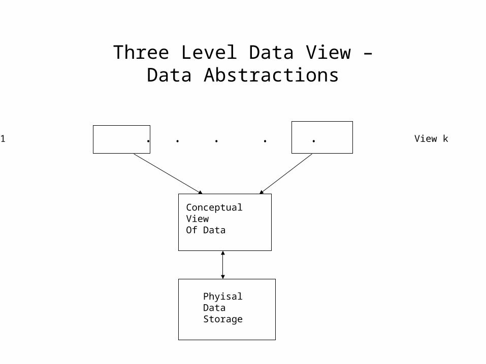
Three Level Data View –Data Abstractions
View1 View k
Conceptual View Of Data
Phyisal Data Storage
. . . . .
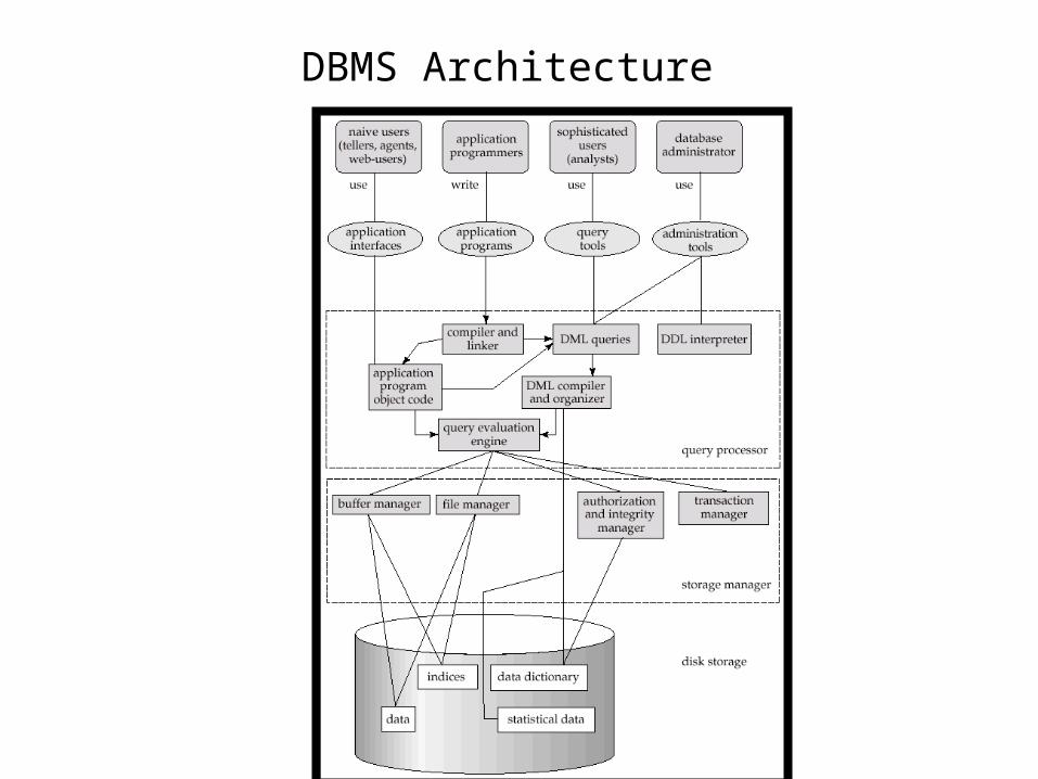
DBMS Architecture
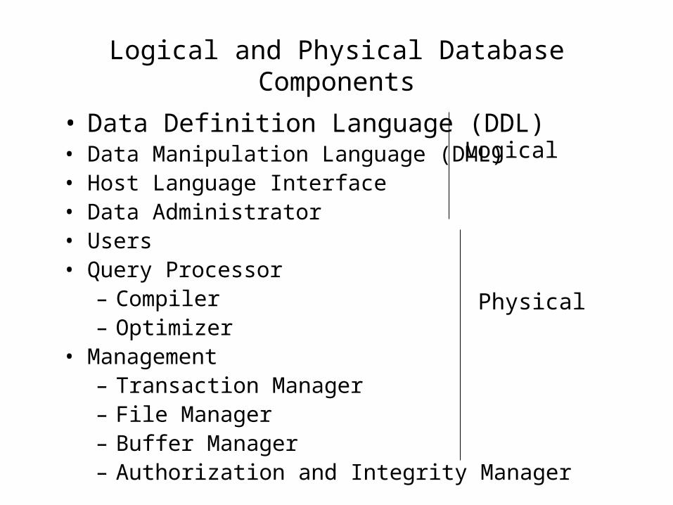
Logical and Physical Database Components
• Data Definition Language (DDL)• Data Manipulation Language (DML)• Host Language Interface• Data Administrator• Users• Query Processor
– Compiler– Optimizer
• Management– Transaction Manager– File Manager– Buffer Manager– Authorization and Integrity Manager
Logical
Physical
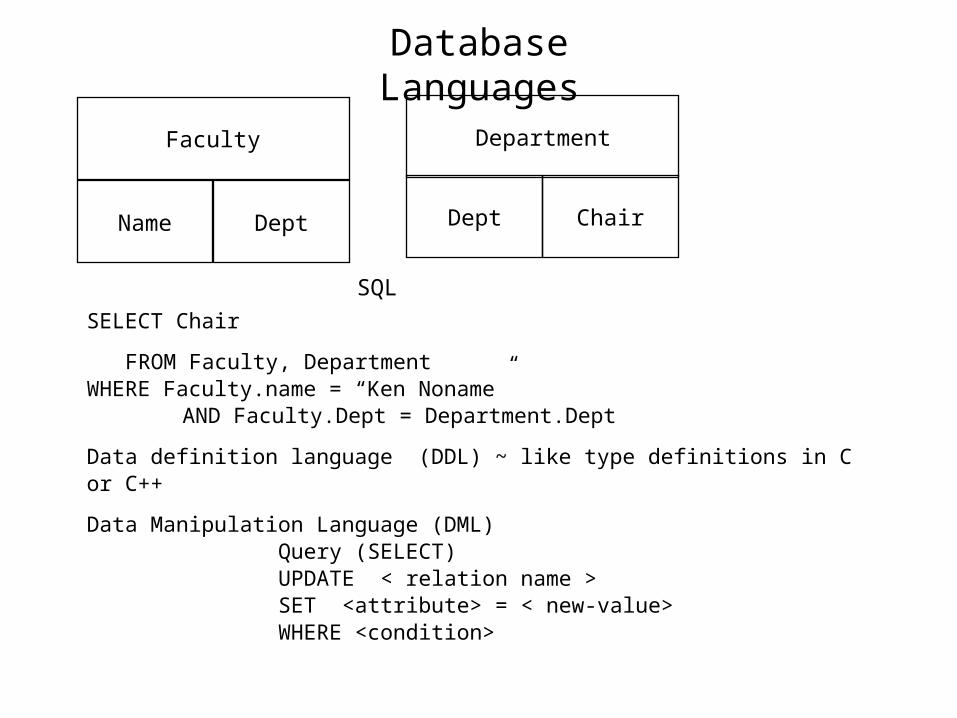
Database Languages
Faculty
Name Dept
Department
Dept Chair
SQL
SELECT Chair
FROM Faculty, DepartmentWHERE Faculty.name = “Ken Noname”
AND Faculty.Dept = Department.Dept
Data definition language (DDL) ~ like type definitions in C or C++
Data Manipulation Language (DML)Query (SELECT)UPDATE < relation name >SET <attribute> = < new-value>WHERE <condition>
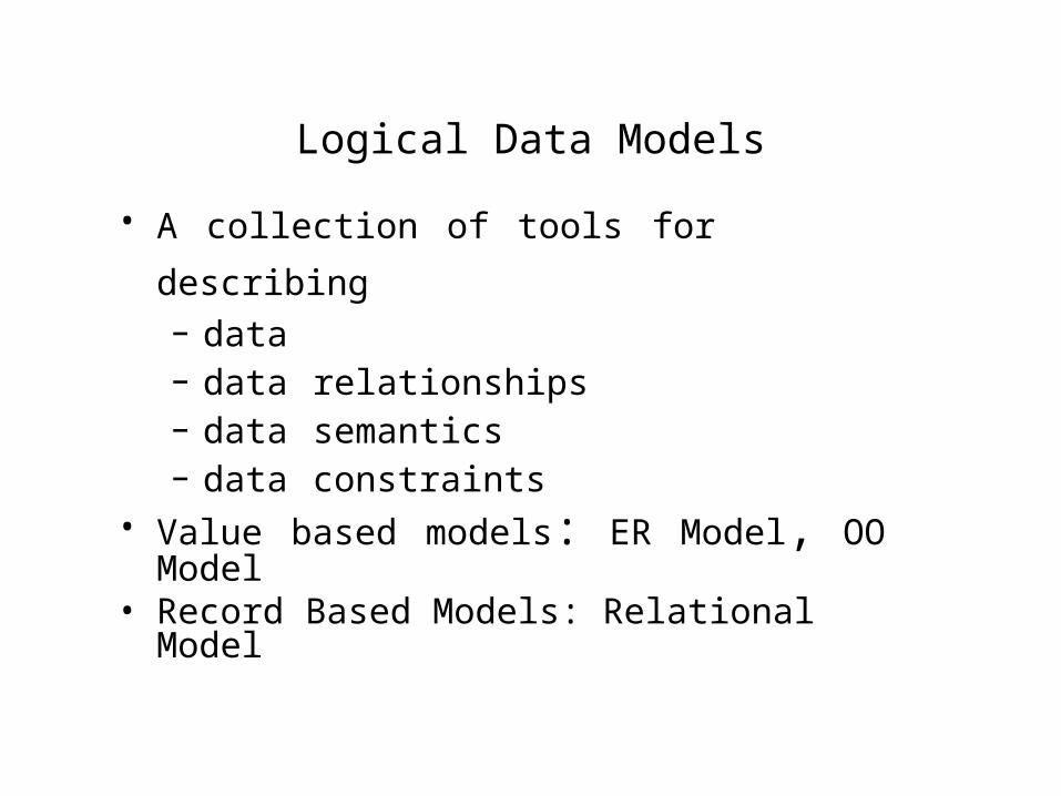
Logical Data Models
• A collection of tools for describing – data – data relationships– data semantics– data constraints
• Value based models: ER Model, OO Model• Record Based Models: Relational Model
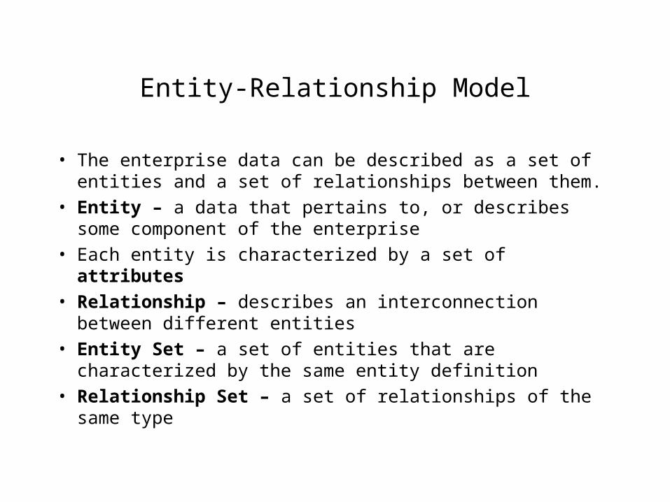
Entity-Relationship Model
• The enterprise data can be described as a set of entities and a set of relationships between them.
• Entity – a data that pertains to, or describes some component of the enterprise
• Each entity is characterized by a set of attributes
• Relationship – describes an interconnection between different entities
• Entity Set – a set of entities that are characterized by the same entity definition
• Relationship Set – a set of relationships of the same type
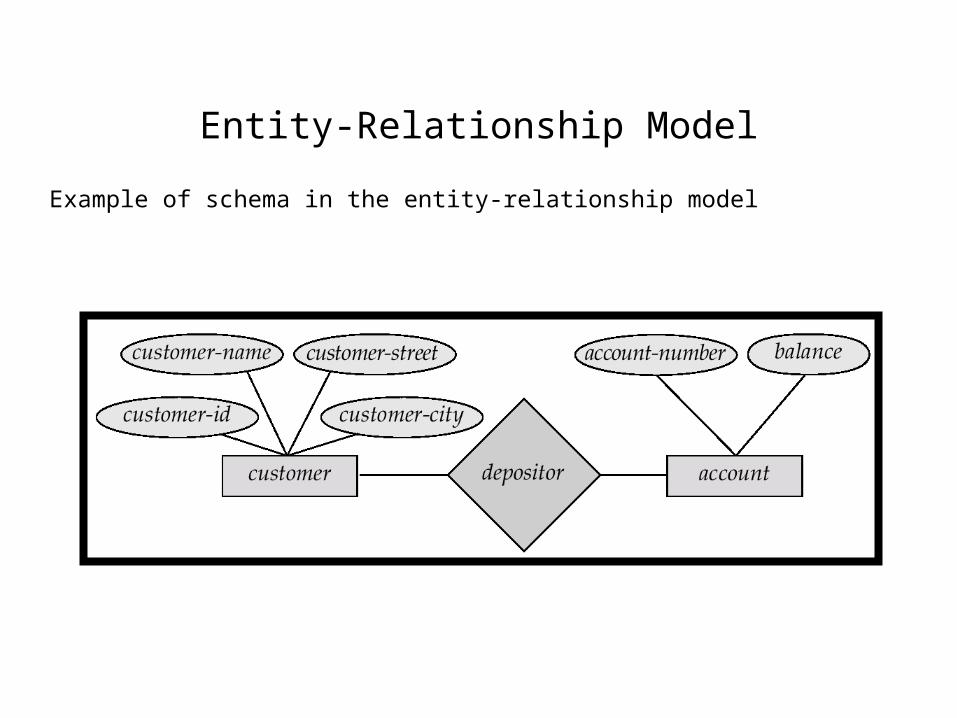
Entity-Relationship Model
Example of schema in the entity-relationship model
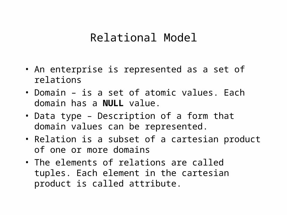
Relational Model
• An enterprise is represented as a set of relations
• Domain – is a set of atomic values. Each domain has a NULL value.
• Data type – Description of a form that domain values can be represented.
• Relation is a subset of a cartesian product of one or more domains
• The elements of relations are called tuples. Each element in the cartesian product is called attribute.
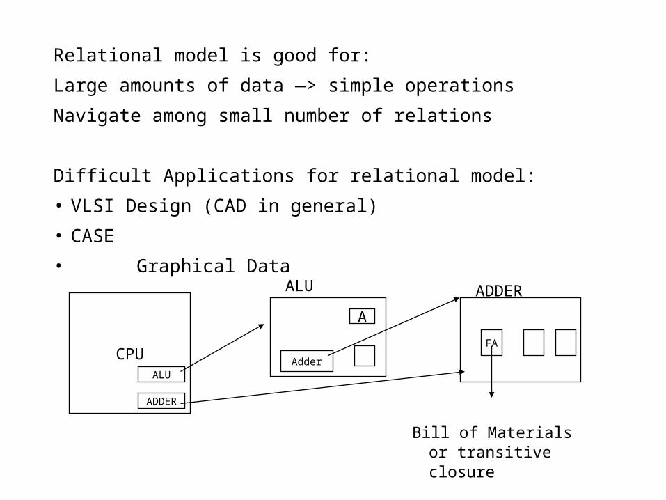
Relational model is good for:
Large amounts of data —> simple operations
Navigate among small number of relations
Difficult Applications for relational model:
• VLSI Design (CAD in general)
• CASE
• Graphical Data
CPUALU
ADDER
Adder
A
FA
ALU ADDER
Bill of Materials or transitive closure
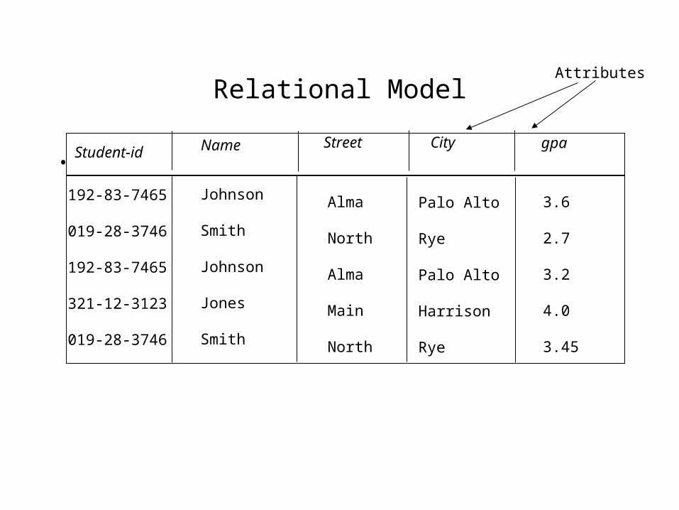
Relational Model
• Example of tabular data in the relational modelNameStudent-id
Street City gpa
Johnson
Smith
Johnson
Jones
Smith
192-83-7465
019-28-3746
192-83-7465
321-12-3123
019-28-3746
Alma
North
Alma
Main
North
Palo Alto
Rye
Palo Alto
Harrison
Rye
3.6
2.7
3.2
4.0
3.45
Attributes
Relational Algebra
Lecture 2
Relational Model
• Basic Notions• Fundamental Relational Algebra Operations• Additional Relational Algebra Operations• Extended Relational Algebra Operations• Null Values• Modification of the Database• Views• Bags and Bag operations
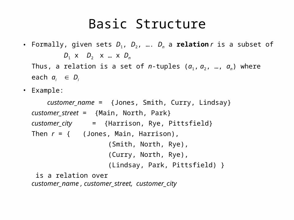
Basic Structure
• Formally, given sets D1, D2, …. Dn a relation r is a subset of
D1 x D2 x … x Dn
Thus, a relation is a set of n-tuples (a1, a2, …, an) where each ai Di
• Example:
customer_name = {Jones, Smith, Curry, Lindsay}
customer_street = {Main, North, Park}
customer_city = {Harrison, Rye, Pittsfield}
Then r = { (Jones, Main, Harrison),
(Smith, North, Rye),
(Curry, North, Rye),
(Lindsay, Park, Pittsfield) }
is a relation over customer_name , customer_street, customer_city
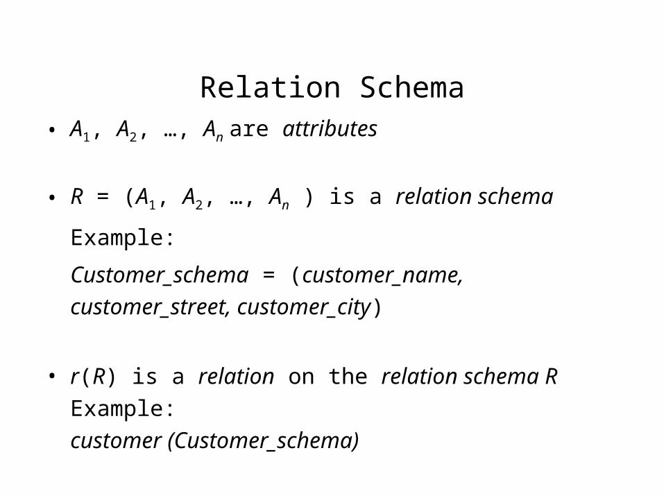
Relation Schema• A1, A2, …, An are attributes
• R = (A1, A2, …, An ) is a relation schema
Example:
Customer_schema = (customer_name, customer_street,
customer_city)
• r(R) is a relation on the relation schema R
Example:
customer (Customer_schema)
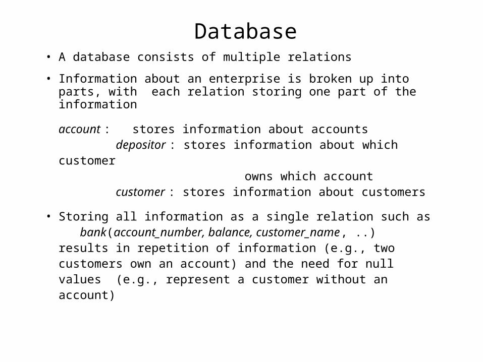
Database• A database consists of multiple relations
• Information about an enterprise is broken up into parts, with each relation storing one part of the information
account : stores information about accounts depositor : stores information about which customer owns which account customer : stores information about customers
• Storing all information as a single relation such as bank(account_number, balance, customer_name, ..)results in repetition of information (e.g., two customers own an account) and the need for null values (e.g., represent a customer without an account)
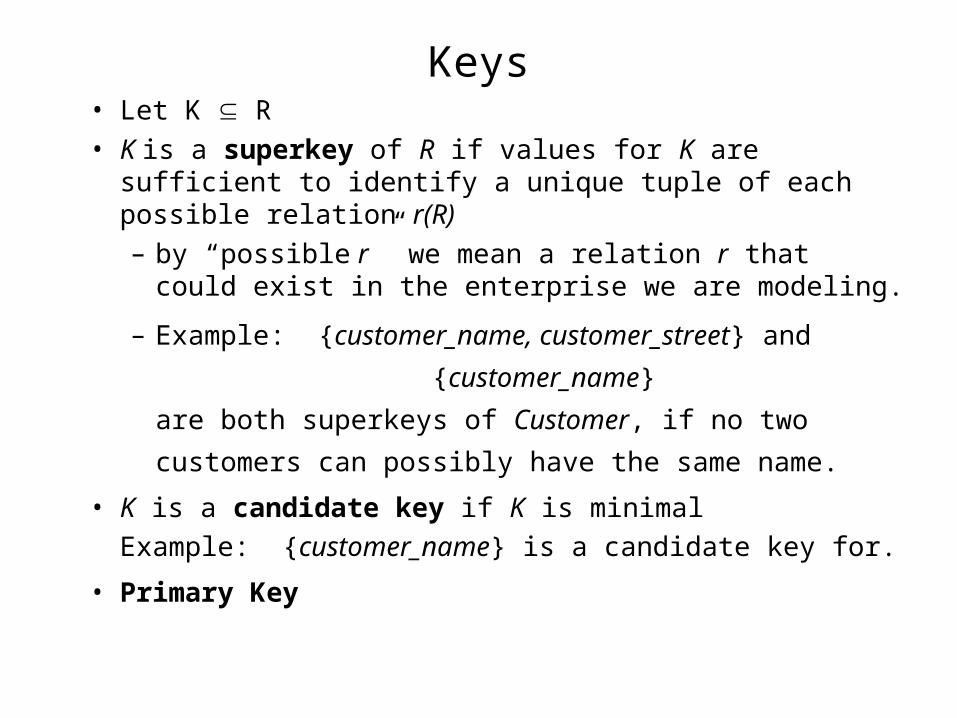
Keys• Let K R
• K is a superkey of R if values for K are sufficient to identify a unique tuple of each possible relation r(R)
– by “possible r ” we mean a relation r that could exist in the enterprise we are modeling.
– Example: {customer_name, customer_street} and
{customer_name}
are both superkeys of Customer, if no two customers can
possibly have the same name.
• K is a candidate key if K is minimal
Example: {customer_name} is a candidate key for.
• Primary Key
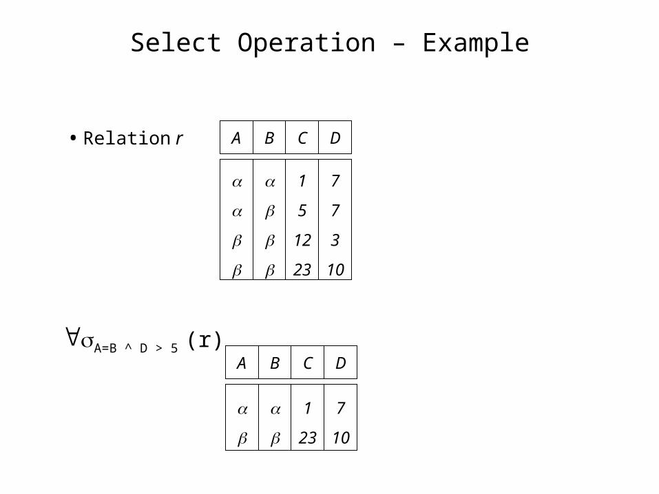
Select Operation – Example
• Relation r A B C D
1
5
12
23
7
7
3
10
A=B ^ D > 5 (r)A B C D
1
23
7
10
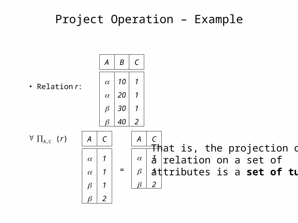
Project Operation – Example
• Relation r:
A B C
10
20
30
40
1
1
1
2
A C
1
1
1
2
=
A C
1
1
2
A,C (r)That is, the projection ofa relation on a set of attributes is a set of tuples
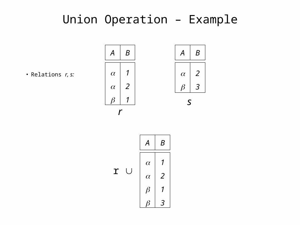
Union Operation – Example
• Relations r, s:
r s:
A B
1
2
1
A B
2
3
rs
A B
1
2
1
3
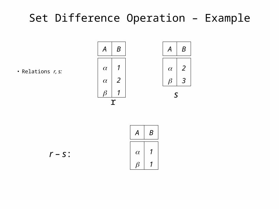
Set Difference Operation – Example
• Relations r, s:
r – s:
A B
1
2
1
A B
2
3
s
A B
1
1
r
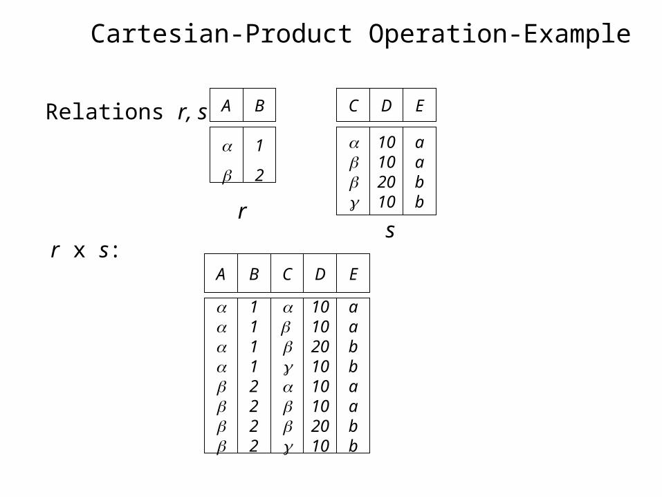
Cartesian-Product Operation-Example
Relations r, s:
r x s:
A B
1
2
A B
11112222
C D
1010201010102010
E
aabbaabb
C D
10102010
E
aabbr
s
Additional Operations
We define additional operations that do not add any powerto the relational algebra, but that simplify common queries.
• Set intersection• Natural join• Division• Assignment
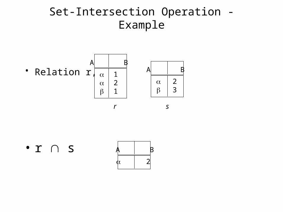
Set-Intersection Operation - Example
• Relation r, s:
• r s
A B
121
A B
23
r s
A B
2
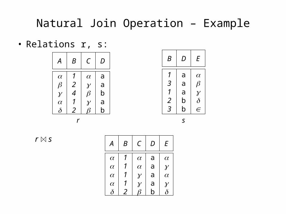
Natural Join Operation – Example
• Relations r, s:
A B
12412
C D
aabab
B
13123
D
aaabb
E
r
A B
11112
C D
aaaab
E
s
r s
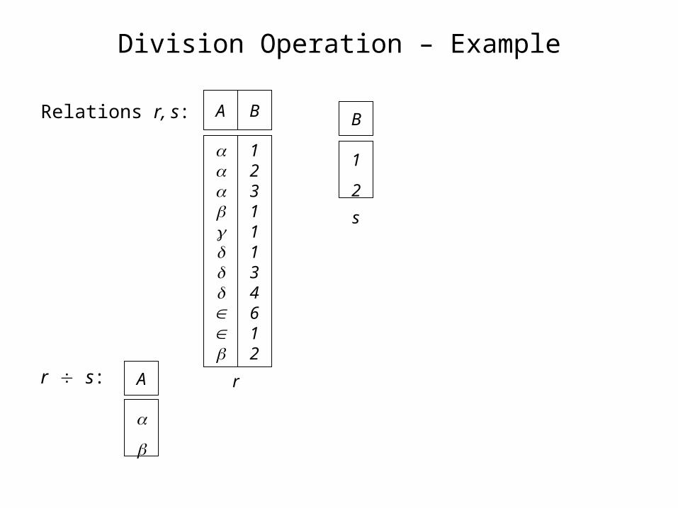
Division Operation – Example
Relations r, s:
r s: A
B
1
2
A B
12311134612
r
s
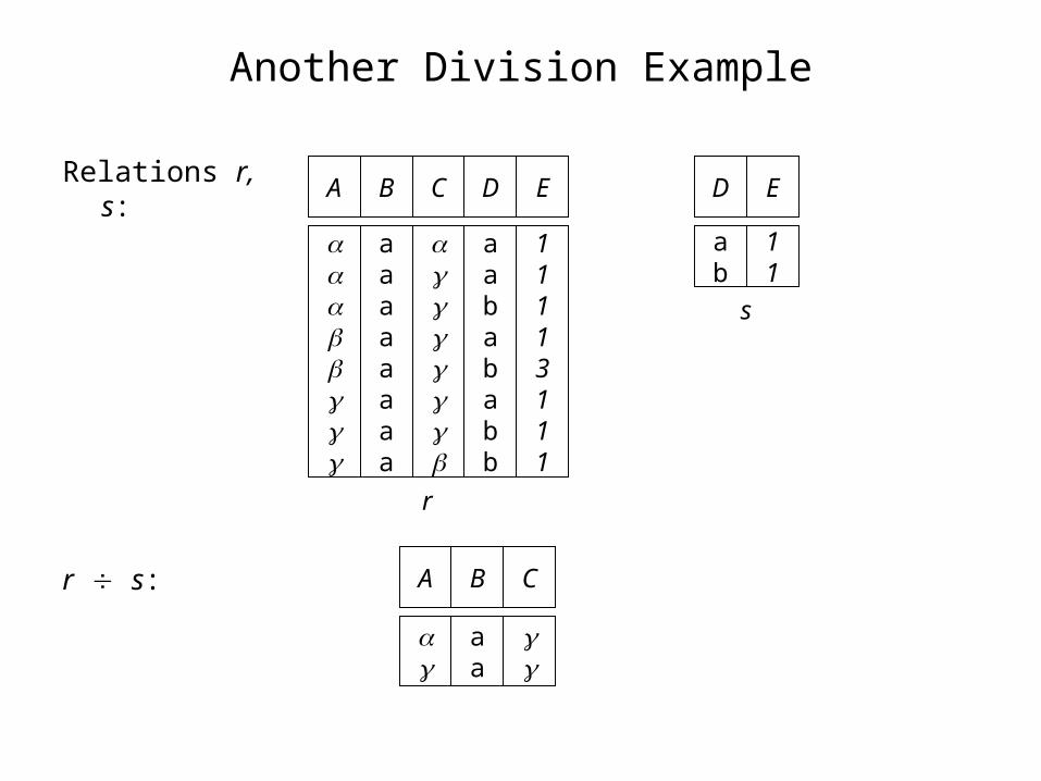
Another Division Example
A B
aaaaaaaa
C D
aabababb
E
11113111
Relations r, s:
r s:
D
ab
E
11
A B
aa
C
r
s
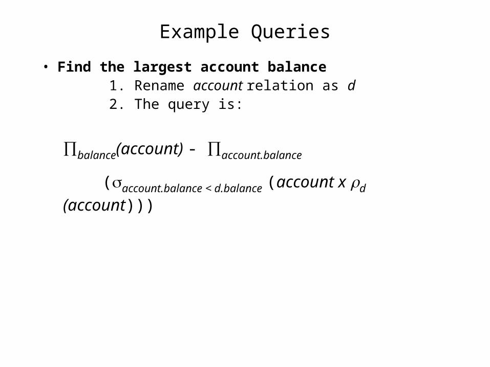
Example Queries
• Find the largest account balance 1. Rename account relation as d 2. The query is:
balance(account) - account.balance
(account.balance < d.balance (account x d (account)))
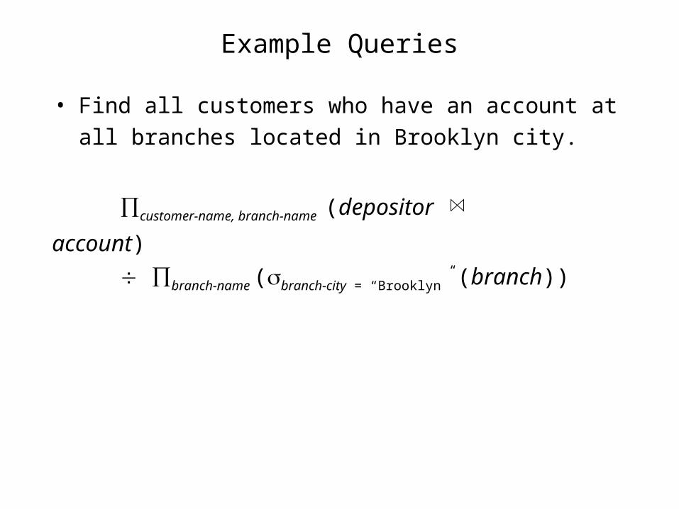
• Find all customers who have an account at all branches
located in Brooklyn city.
Example Queries
customer-name, branch-name (depositor account)
branch-name (branch-city = “Brooklyn” (branch))
Extended Relational-Algebra-Operations
• Generalized Projection
• Outer Join
• Aggregate Functions
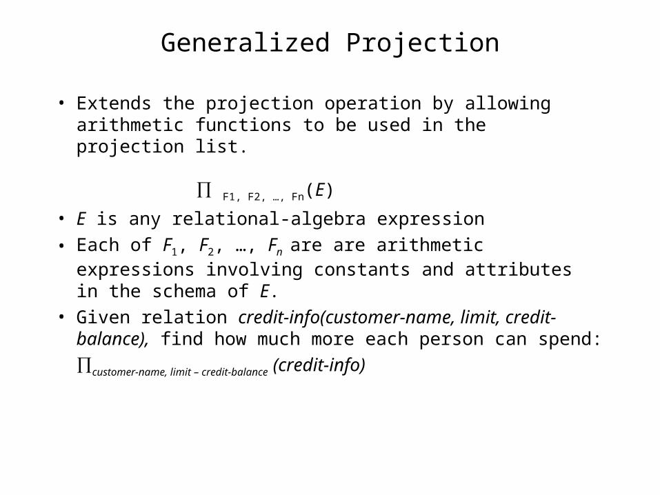
Generalized Projection
• Extends the projection operation by allowing arithmetic functions to be used in the projection list.
F1, F2, …, Fn(E)
• E is any relational-algebra expression
• Each of F1, F2, …, Fn are are arithmetic expressions involving constants and attributes in the schema of E.
• Given relation credit-info(customer-name, limit, credit-balance), find how much more each person can spend:
customer-name, limit – credit-balance (credit-info)
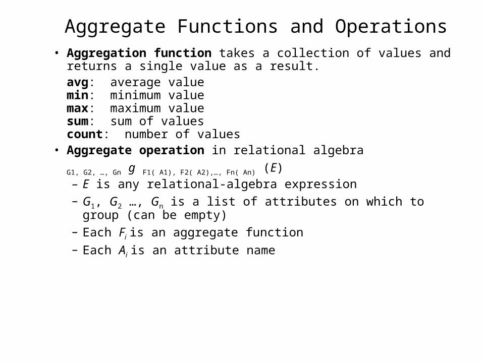
Aggregate Functions and Operations• Aggregation function takes a collection of values and returns a single
value as a result.avg: average valuemin: minimum valuemax: maximum valuesum: sum of valuescount: number of values
• Aggregate operation in relational algebra
G1, G2, …, Gn g F1( A1), F2( A2),…, Fn( An) (E)– E is any relational-algebra expression– G1, G2 …, Gn is a list of attributes on which to group (can be empty)– Each Fi is an aggregate function– Each Ai is an attribute name
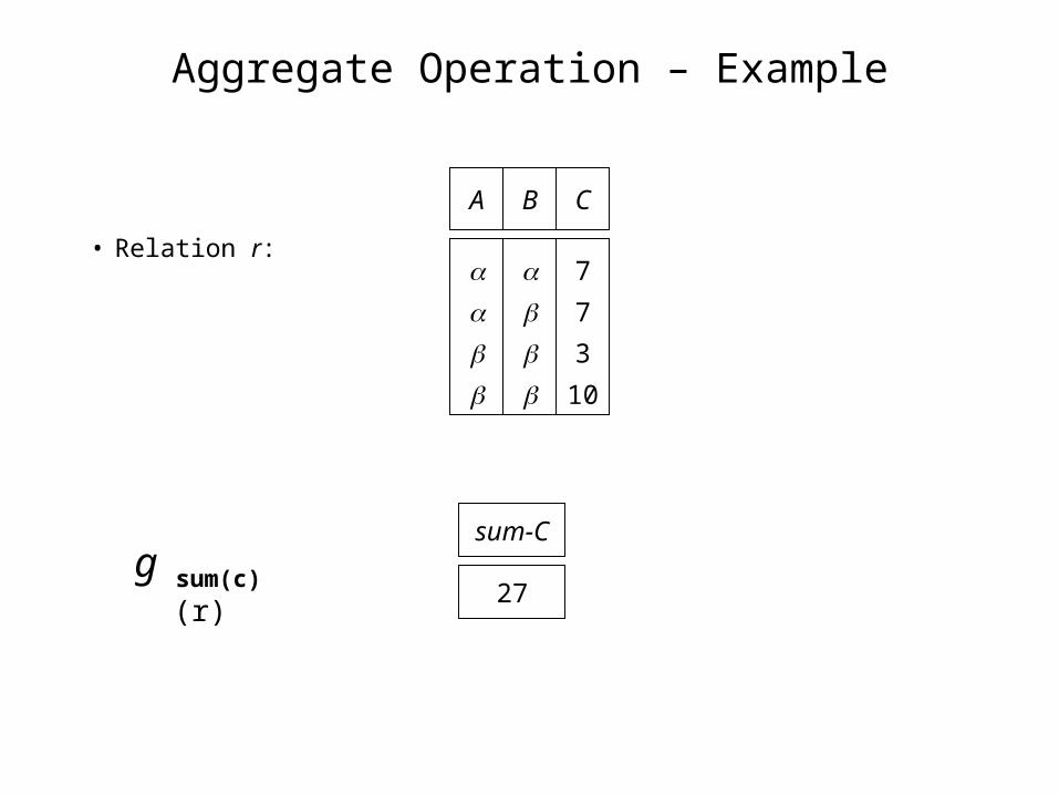
Aggregate Operation – Example
• Relation r:
A B
C
7
7
3
10
g sum(c) (r)sum-C
27
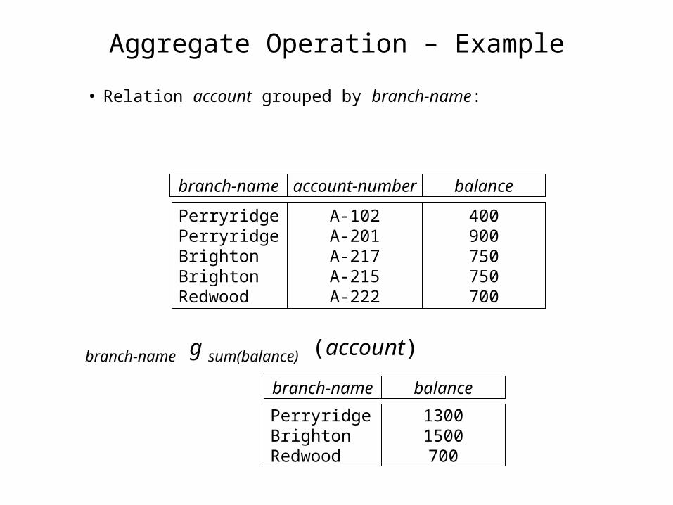
Aggregate Operation – Example
• Relation account grouped by branch-name:
branch-name g sum(balance) (account)
branch-name account-number balance
PerryridgePerryridgeBrightonBrightonRedwood
A-102A-201A-217A-215A-222
400900750750700
branch-name balance
PerryridgeBrightonRedwood
13001500700
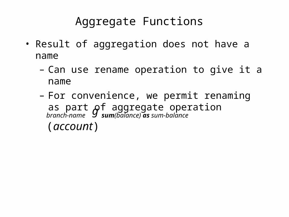
Aggregate Functions • Result of aggregation does not have a name
– Can use rename operation to give it a name
– For convenience, we permit renaming as part of aggregate operation
branch-name g sum(balance) as sum-balance (account)
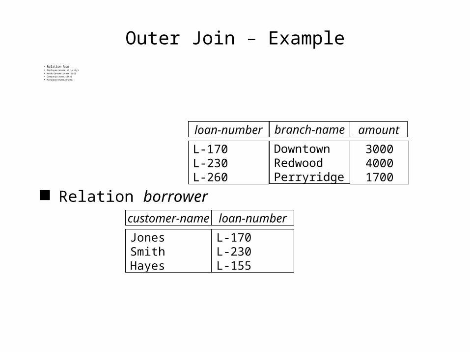
Outer Join – Example• Relation loan• Employee(ename,str,city)• Works(ename,cname,sal)• Company(cname,city)• Manages(ename,mname)
Relation borrowercustomer-name loan-number
JonesSmithHayes
L-170L-230L-155
300040001700
loan-number amount
L-170L-230L-260
branch-name
DowntownRedwoodPerryridge
SQLLecture 3
SQL• Data Definition• Basic Query Structure• Set Operations• Aggregate Functions• Null Values• Nested Subqueries• Complex Queries • Views
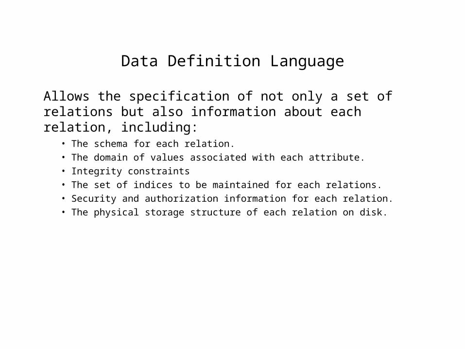
Data Definition Language
• The schema for each relation.
• The domain of values associated with each attribute.
• Integrity constraints
• The set of indices to be maintained for each relations.
• Security and authorization information for each relation.
• The physical storage structure of each relation on disk.
Allows the specification of not only a set of relations but also information about each relation, including:
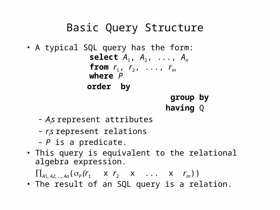
Basic Query Structure • A typical SQL query has the form:
select A1, A2, ..., An
from r1, r2, ..., rm
where P order by group by having Q
– Ais represent attributes– ris represent relations– P is a predicate.
• This query is equivalent to the relational algebra expression.
A1, A2, ..., An(P (r1 x r2 x ... x rm))• The result of an SQL query is a relation.
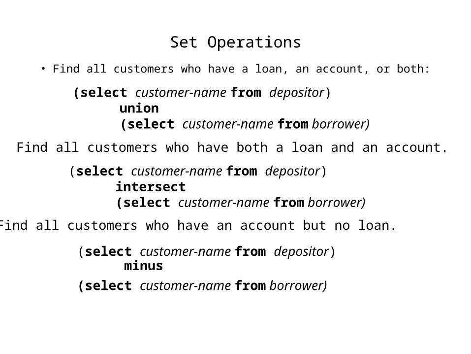
Set Operations
• Find all customers who have a loan, an account, or both:
(select customer-name from depositor)minus
(select customer-name from borrower)
(select customer-name from depositor)intersect(select customer-name from borrower)
Find all customers who have an account but no loan.
(select customer-name from depositor)union(select customer-name from borrower)
Find all customers who have both a loan and an account.
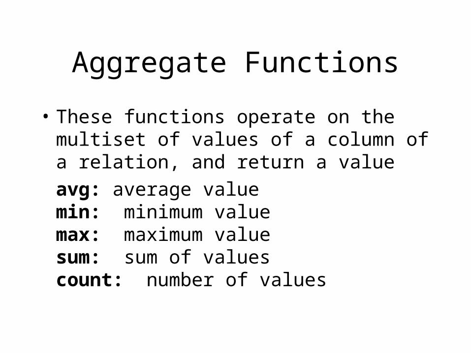
Aggregate Functions
• These functions operate on the multiset of values of a column of a relation, and return a value
avg: average valuemin: minimum valuemax: maximum valuesum: sum of valuescount: number of values
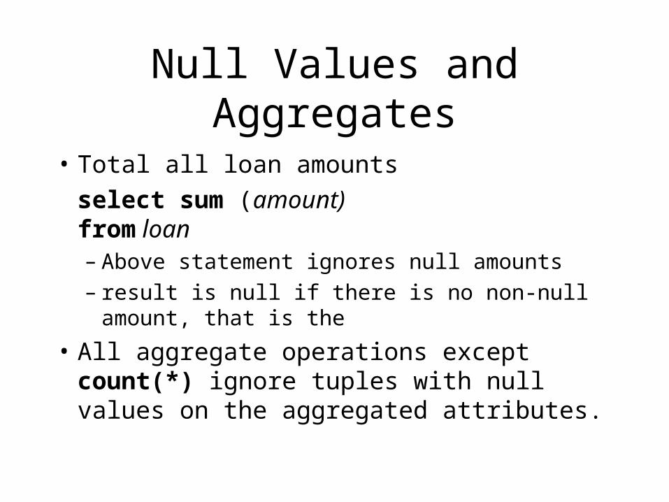
Null Values and Aggregates
• Total all loan amounts
select sum (amount)from loan
– Above statement ignores null amounts– result is null if there is no non-null amount, that is
the
• All aggregate operations except count(*) ignore tuples with null values on the aggregated attributes.
Nested Subqueries
• SQL provides a mechanism for the nesting of subqueries.
• A subquery is a select-from-where expression that is nested within another query.
• A common use of subqueries is to perform tests for set membership, set comparisons, and set cardinality.
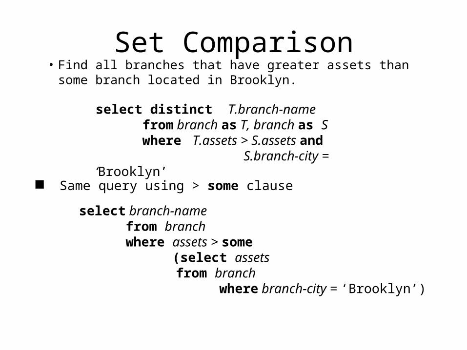
Set Comparison• Find all branches that have greater assets than some branch located in
Brooklyn.
Same query using > some clause
select branch-namefrom branchwhere assets > some (select assets from branch
where branch-city = ‘Brooklyn’)
select distinct T.branch-namefrom branch as T, branch as Swhere T.assets > S.assets and S.branch-city = ‘Brooklyn’
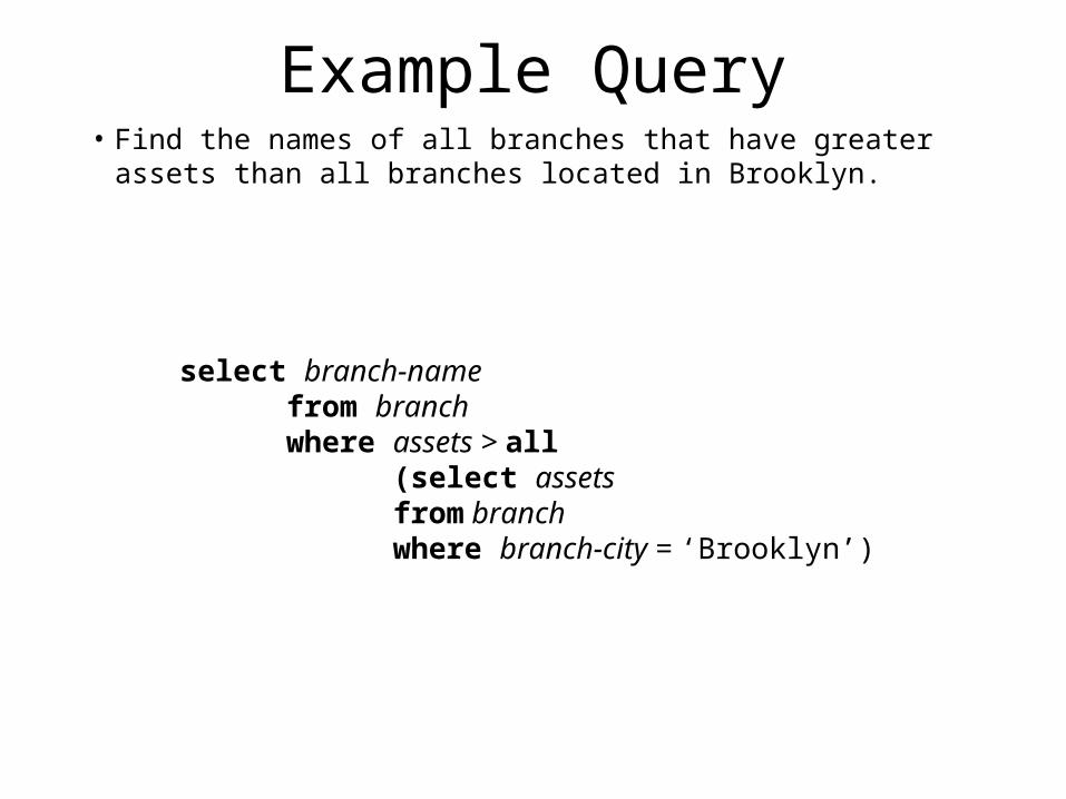
Example Query• Find the names of all branches that have greater assets than
all branches located in Brooklyn.
select branch-namefrom branchwhere assets > all
(select assetsfrom branchwhere branch-city = ‘Brooklyn’)
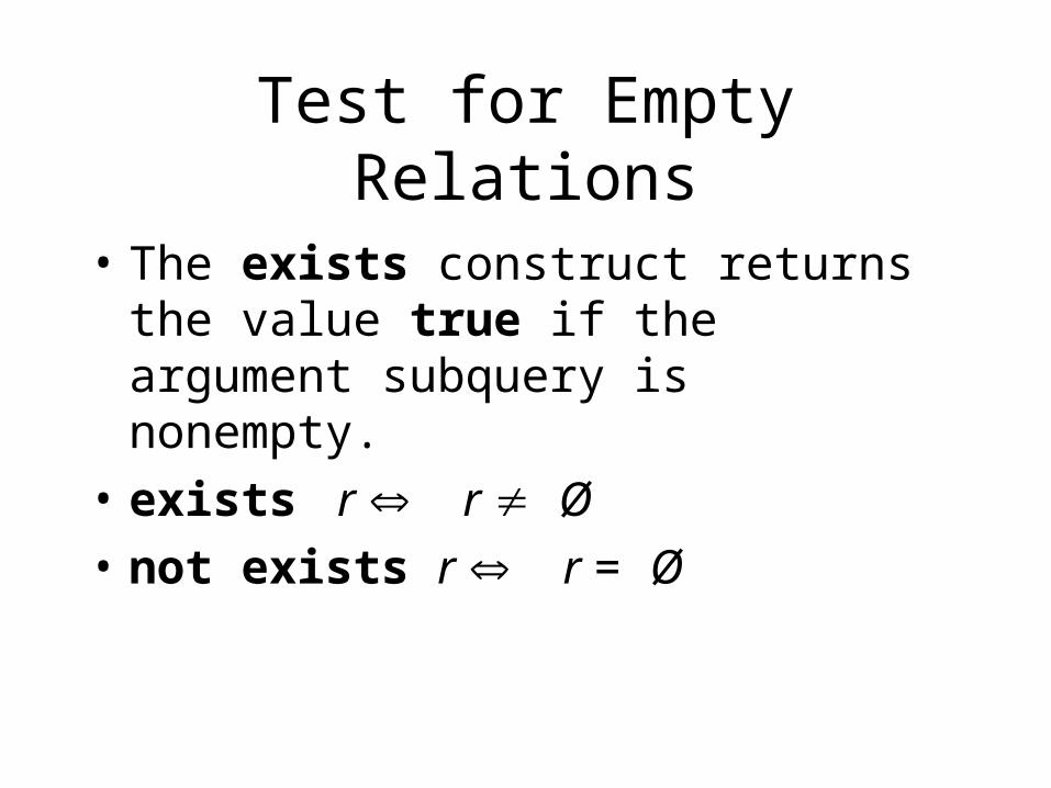
Test for Empty Relations
• The exists construct returns the value true if the argument subquery is nonempty.
• exists r r Ø
• not exists r r = Ø
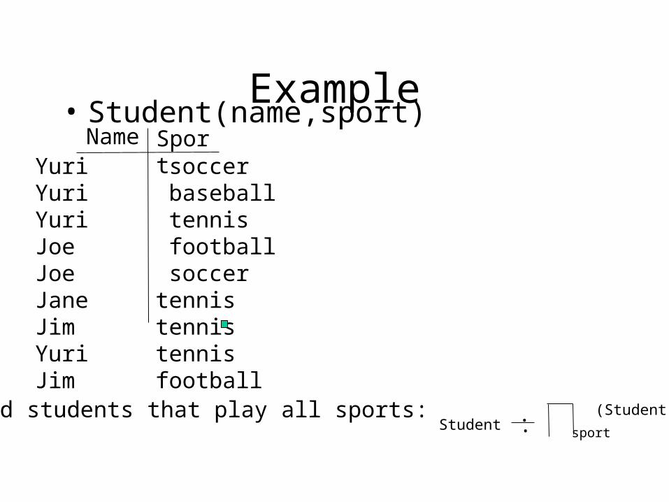
Example• Student(name,sport)
Name SportYuri soccerYuri baseballYuri tennisJoe footballJoe soccerJane tennisJim tennisYuri tennisJim footballFind students that play all sports:
sport
(Student)Student ..
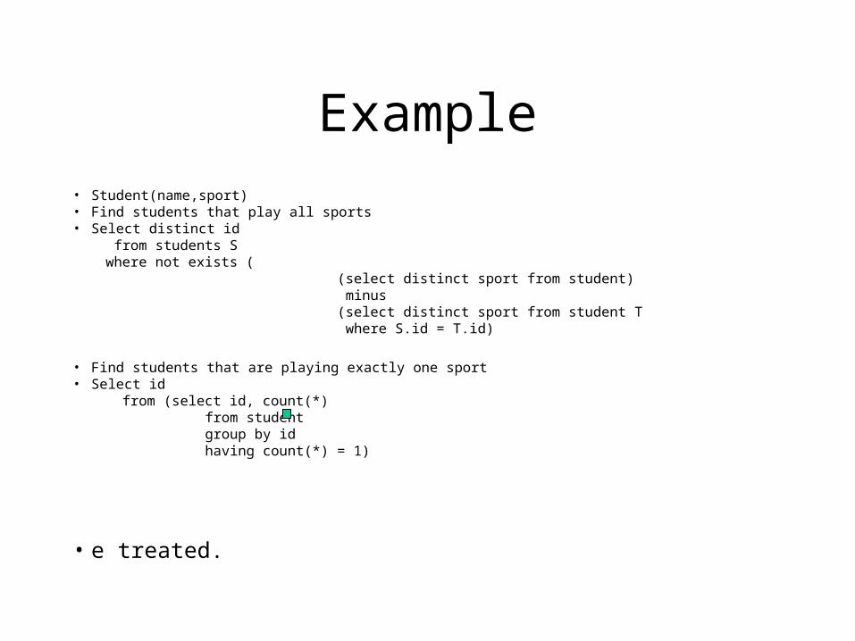
Example• Student(name,sport)• Find students that play all sports• Select distinct id from students S where not exists ( (select distinct sport from student) minus (select distinct sport from student T where S.id = T.id)
• Find students that are playing exactly one sport• Select id from (select id, count(*) from student group by id having count(*) = 1)
• e treated.
Entity-Relationship Model
Lecture 5
ER Model Components
• Entity Sets
• Attributes
• Relationships
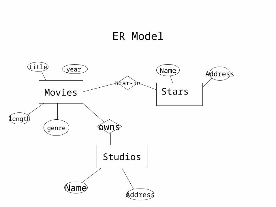
ER Model
Movies
Studios
title
length
genre owns
Star-in
Stars
year
NameAddress
Name Address
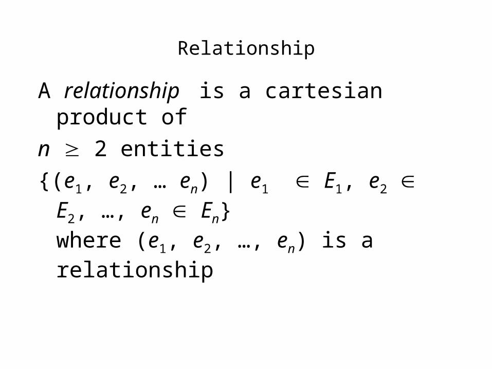
Relationship
A relationship is a cartesian product of
n 2 entities
{(e1, e2, … en) | e1 E1, e2 E2, …, en En}where (e1, e2, …, en) is a relationship
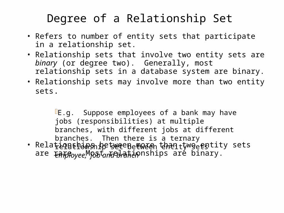
Degree of a Relationship Set
• Refers to number of entity sets that participate in a relationship set.
• Relationship sets that involve two entity sets are binary (or degree two). Generally, most relationship sets in a database system are binary.
• Relationship sets may involve more than two entity sets.
• Relationships between more than two entity sets are rare. Most relationships are binary.
E.g. Suppose employees of a bank may have jobs (responsibilities) at multiple branches, with different jobs at different branches. Then there is a ternary relationship set between entity sets employee, job and branch
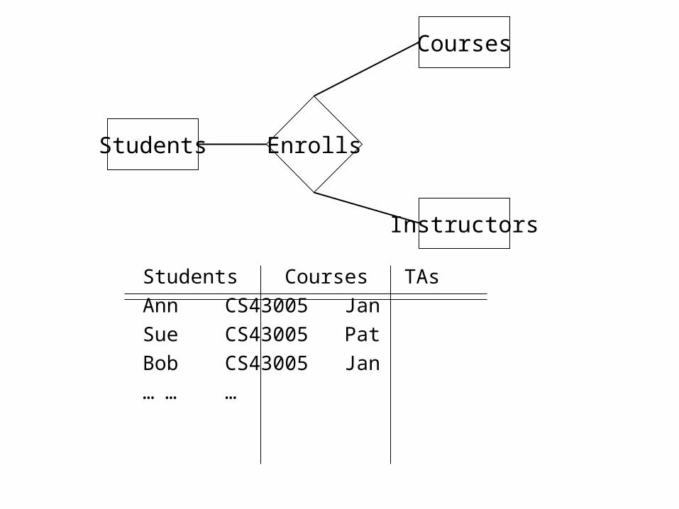
Students Courses TAs
Ann CS43005 Jan
Sue CS43005 Pat
Bob CS43005 Jan
… … …
Students
Courses
Instructors
Enrolls
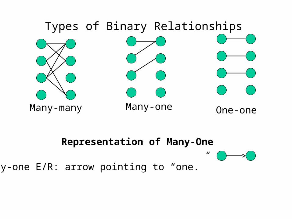
Types of Binary Relationships
Representation of Many-One
Many-many
Many-one E/R: arrow pointing to “one.”
One-oneMany-one
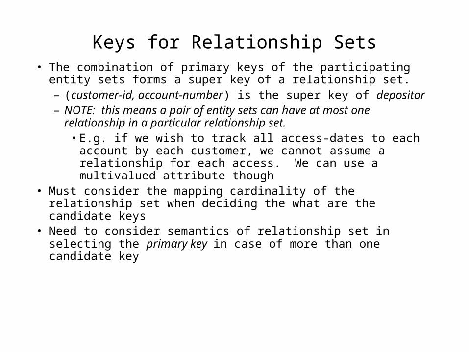
Keys for Relationship Sets• The combination of primary keys of the participating entity sets
forms a super key of a relationship set.– (customer-id, account-number) is the super key of depositor– NOTE: this means a pair of entity sets can have at most one
relationship in a particular relationship set. • E.g. if we wish to track all access-dates to each account
by each customer, we cannot assume a relationship for each access. We can use a multivalued attribute though
• Must consider the mapping cardinality of the relationship set when deciding the what are the candidate keys
• Need to consider semantics of relationship set in selecting the primary key in case of more than one candidate key
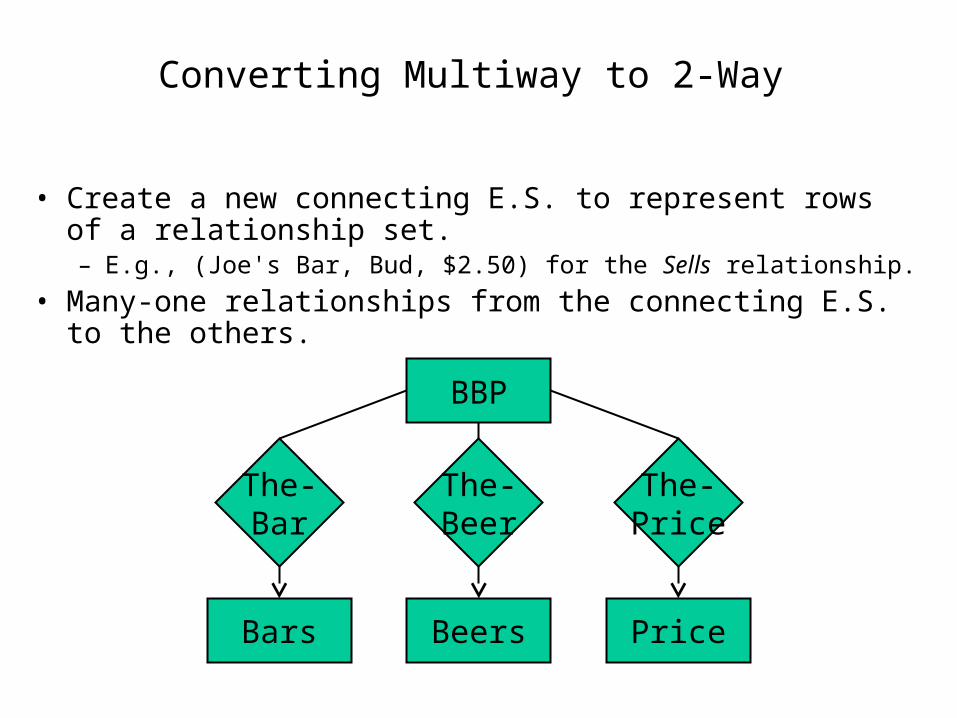
Converting Multiway to 2-Way
• Create a new connecting E.S. to represent rows of a relationship set.– E.g., (Joe's Bar, Bud, $2.50) for the Sells relationship.
• Many-one relationships from the connecting E.S. to the others.
Bars Beers
The-Bar
Price
The-Beer
The-Price
BBP
Specialization
• within an entity set that are distinctive from other entities in the set.
• These subgroupings become lower-level entity sets that have attributes or participate in relationships that do not apply to the higher-level entity set.
• Depicted by a triangle component labeled ISA (E.g. Top-down design process; we designate subgroupings customer “is a” person).
• Attribute inheritance – a lower-level entity set inherits all the attributes and relationship participation of the higher-level entity set to which it is linked.
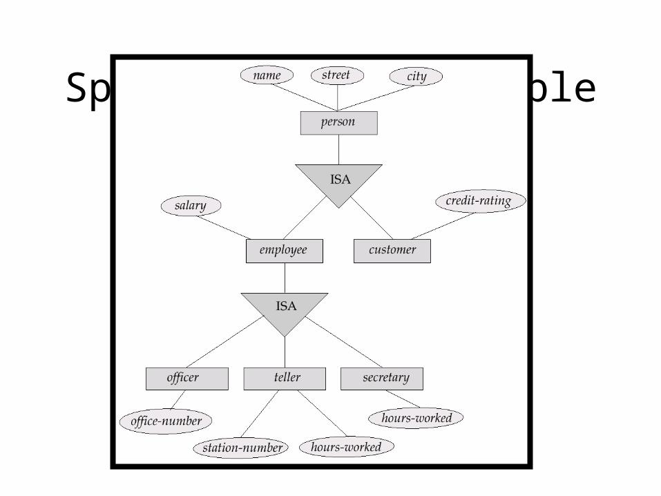
Specialization Example
Generalization
• A bottom-up design process – combine a number of entity sets that share the same features into a higher-level entity set.
• Specialization and generalization are simple inversions of each other; they are represented in an E-R diagram in the same way.
• The terms specialization and generalization are used interchangeably.
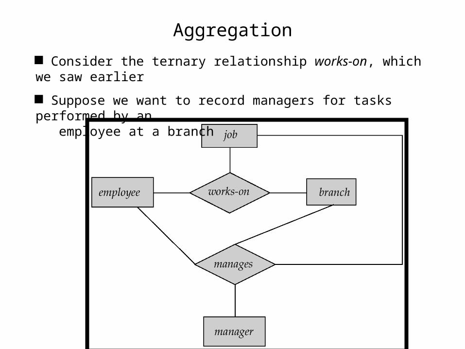
Aggregation
Consider the ternary relationship works-on, which we saw earlier
Suppose we want to record managers for tasks performed by an employee at a branch
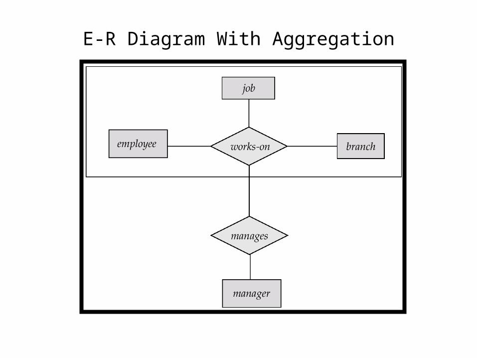
E-R Diagram With Aggregation
Weak Entity Sets
• An entity set that does not have a primary key is referred to as a weak entity set.
• The existence of a weak entity set depends on the existence of a identifying entity set– it must relate to the identifying entity set via a total, one-to-
many relationship set from the identifying to the weak entity set– Identifying relationship depicted using a double diamond
• The discriminator (or partial key) of a weak entity set is the set of attributes that distinguishes among all the entities of a weak entity set.
• The primary key of a weak entity set is formed by the primary key of the strong entity set on which the weak entity set is existence dependent, plus the weak entity set’s discriminator.
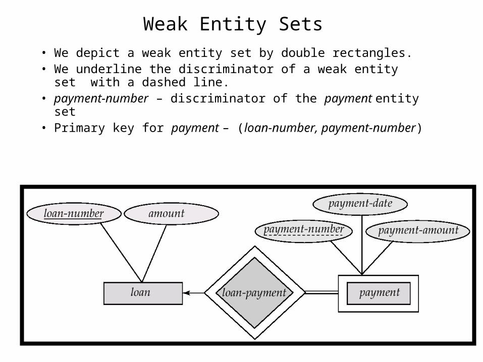
Weak Entity Sets • We depict a weak entity set by double rectangles.• We underline the discriminator of a weak entity set with a
dashed line.• payment-number – discriminator of the payment entity set • Primary key for payment – (loan-number, payment-number)
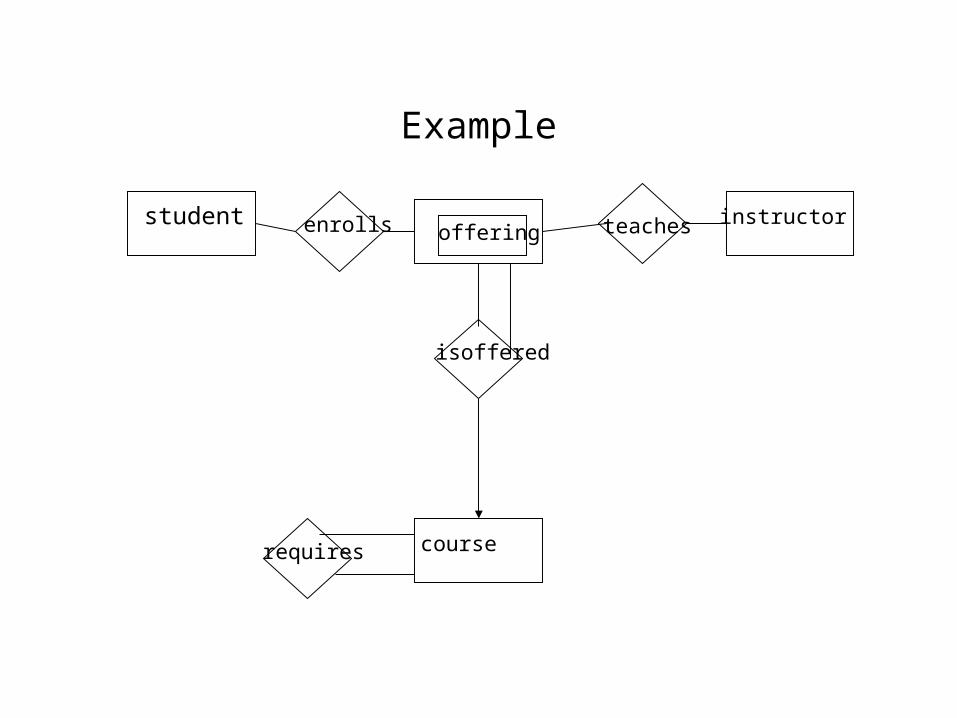
Example
studentoffering
instructor
course
enrolls teaches
isoffered
requires
Reduction of an E-R Schema to Tables
• Primary keys allow entity sets and relationship sets to be expressed uniformly as tables which represent the contents of the database.
• A database which conforms to an E-R diagram can be represented by a collection of tables.
• For each entity set and relationship set there is a unique table which is assigned the name of the corresponding entity set or relationship set.
• Each table has a number of columns (generally corresponding to attributes), which have unique names.
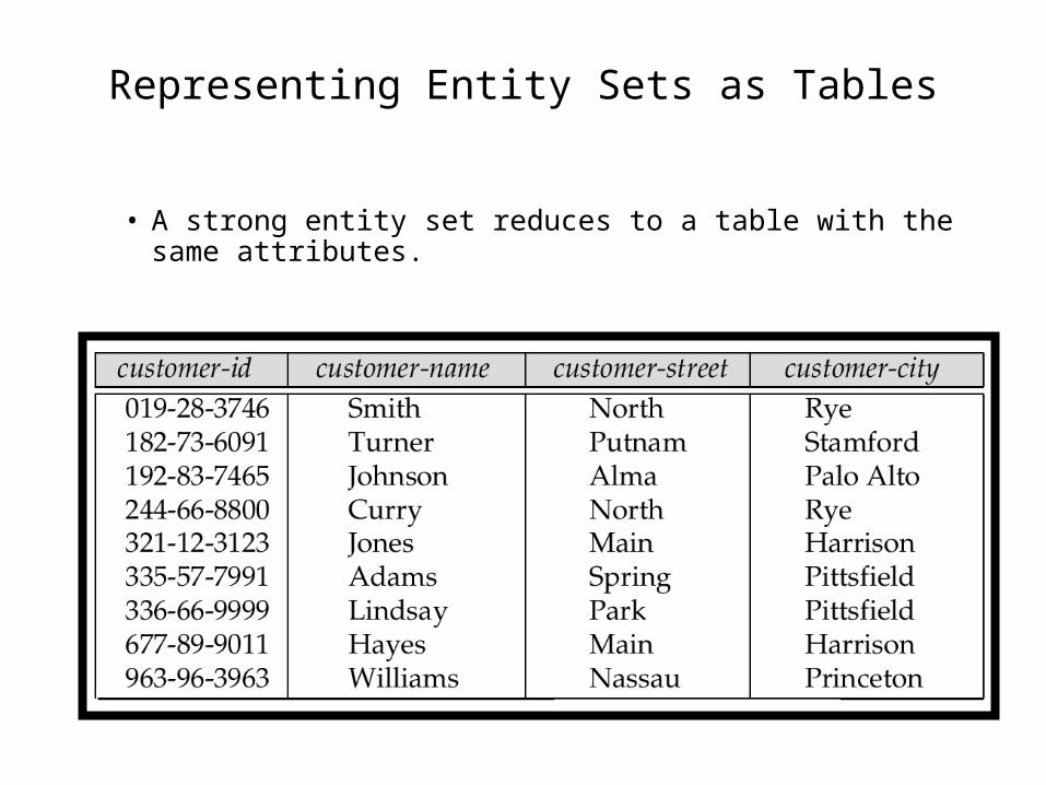
Representing Entity Sets as Tables
• A strong entity set reduces to a table with the same attributes.
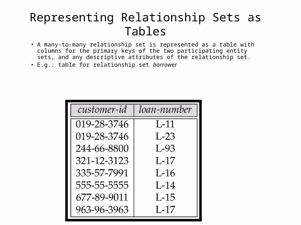
Representing Relationship Sets as Tables
• A many-to-many relationship set is represented as a table with columns for the primary keys of the two participating entity sets, and any descriptive attributes of the relationship set.
• E.g.: table for relationship set borrower
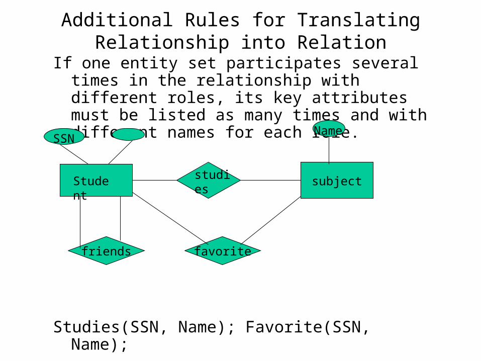
Additional Rules for Translating Relationship into Relation
If one entity set participates several times in the relationship with different roles, its key attributes must be listed as many times and with different names for each role.
Studies(SSN, Name); Favorite(SSN, Name);
Friends(SSN1, SSN2)
subject
friends favorite
Student studies
SSNName
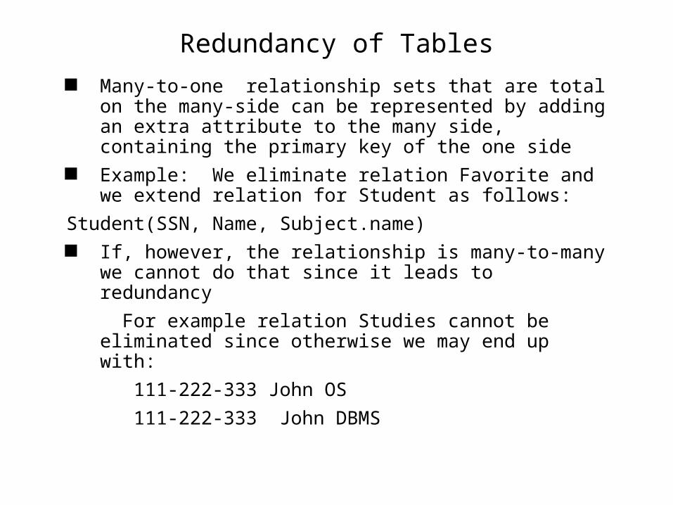
Redundancy of Tables
Many-to-one relationship sets that are total on the many-side can be represented by adding an extra attribute to the many side, containing the primary key of the one side
Example: We eliminate relation Favorite and we extend relation for Student as follows:
Student(SSN, Name, Subject.name) If, however, the relationship is many-to-many we cannot do
that since it leads to redundancy
For example relation Studies cannot be eliminated since otherwise we may end up with:
111-222-333 John OS
111-222-333 John DBMS
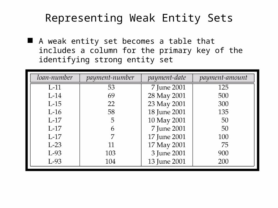
Representing Weak Entity Sets
A weak entity set becomes a table that includes a column for the primary key of the identifying strong entity set
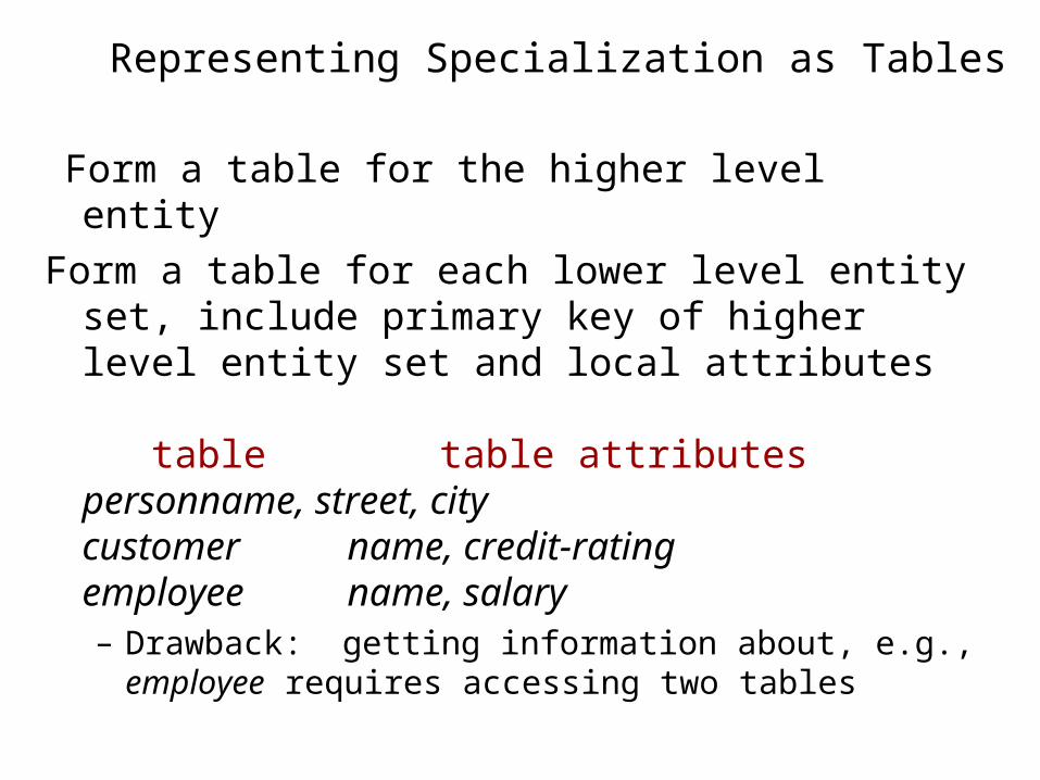
Representing Specialization as Tables
Form a table for the higher level entity
Form a table for each lower level entity set, include primary key of higher level entity set and local attributes
table table attributespersonname, street, city customer name, credit-ratingemployee name, salary– Drawback: getting information about, e.g., employee
requires accessing two tables
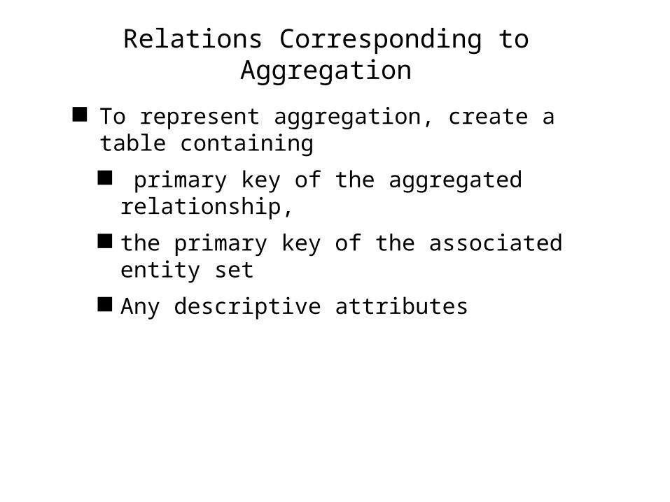
Relations Corresponding to Aggregation
To represent aggregation, create a table containing
primary key of the aggregated relationship,
the primary key of the associated entity set
Any descriptive attributes
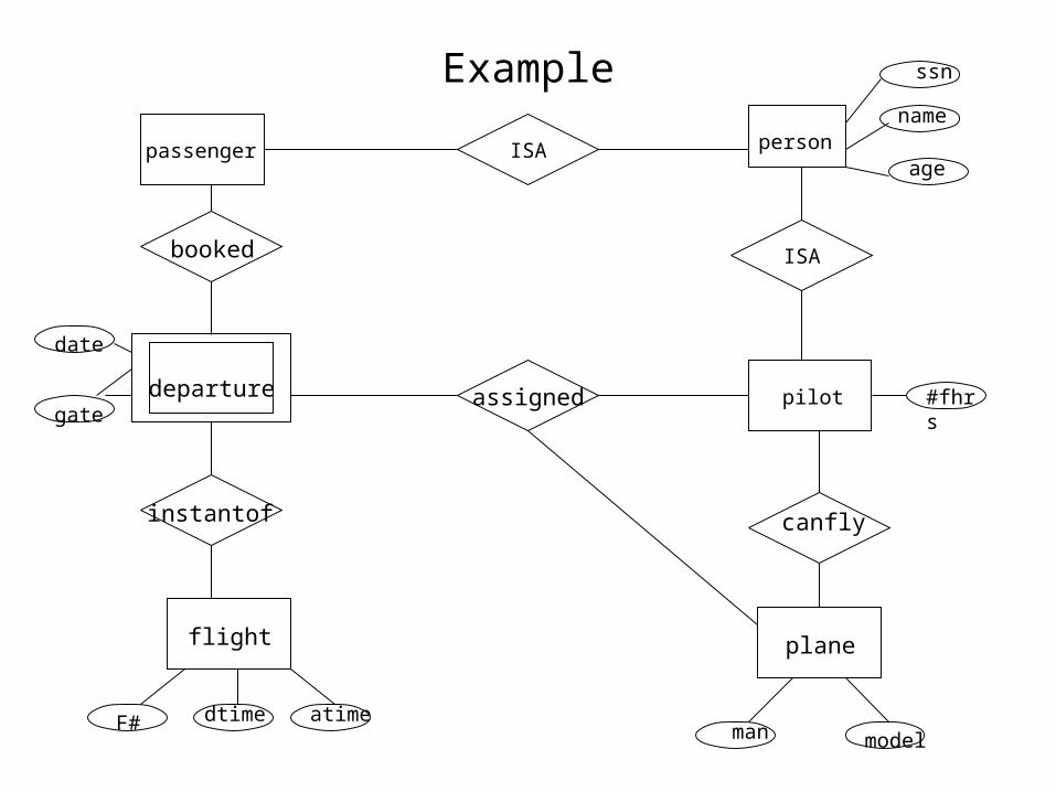
Example
ISA
ISA
passenger person
pilotdeparture
flight
booked
instantof
assigned
canfly
plane
date
gate
F# dtime atime
ssn
name
age
#fhrs
man model
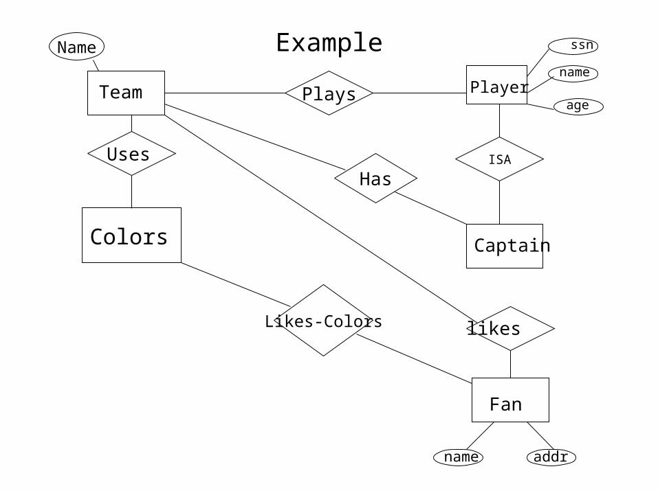
Example
Plays
ISA
Team Player
Captain
Uses
Fan
ssn
name
age
name addr
Name
Colors
likesLikes-Colors
Has
Relational Database Design Theory
Lecture 6
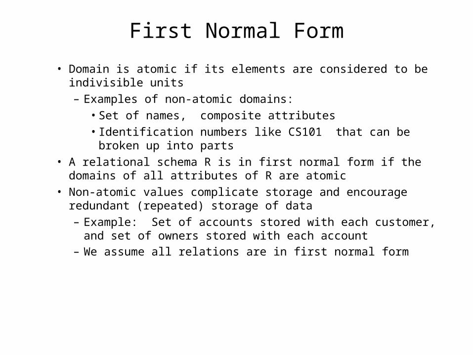
First Normal Form
• Domain is atomic if its elements are considered to be indivisible units– Examples of non-atomic domains:
• Set of names, composite attributes• Identification numbers like CS101 that can be broken up into
parts• A relational schema R is in first normal form if the domains of all
attributes of R are atomic• Non-atomic values complicate storage and encourage redundant
(repeated) storage of data– Example: Set of accounts stored with each customer, and set of
owners stored with each account– We assume all relations are in first normal form
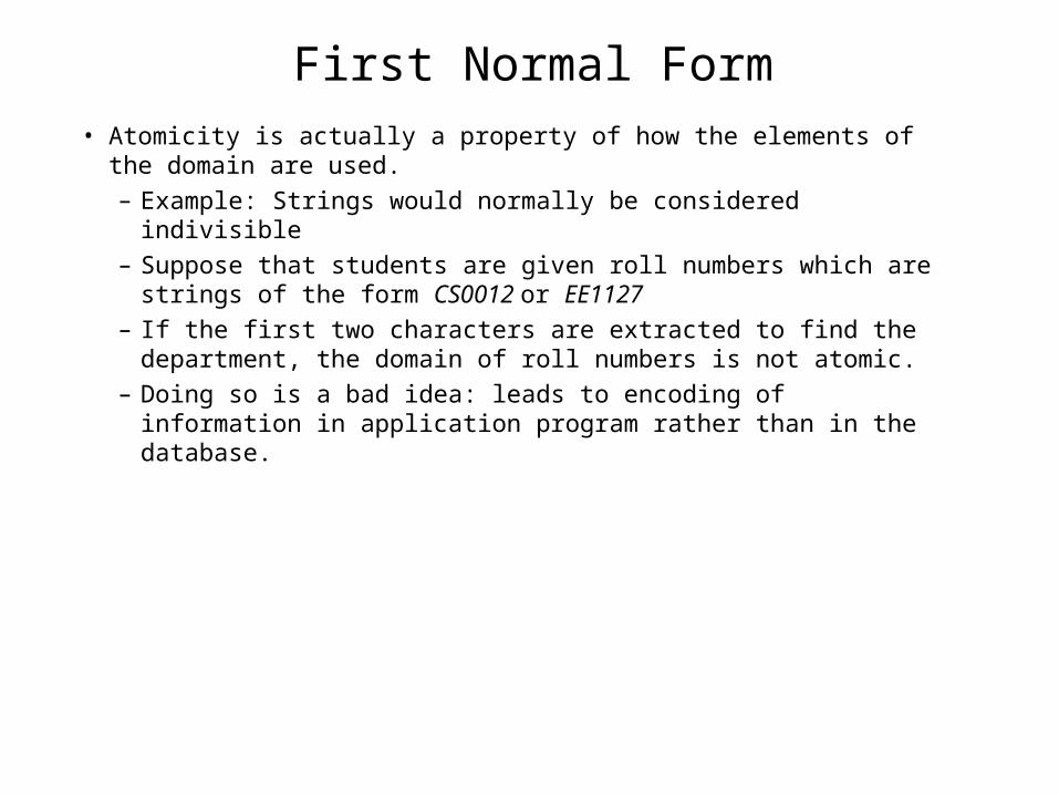
First Normal Form
• Atomicity is actually a property of how the elements of the domain are used.
– Example: Strings would normally be considered indivisible
– Suppose that students are given roll numbers which are strings of the form CS0012 or EE1127
– If the first two characters are extracted to find the department, the domain of roll numbers is not atomic.
– Doing so is a bad idea: leads to encoding of information in application program rather than in the database.
Functional Dependencies
• Constraints on the set of legal relations.
• Require that the value for a certain set of attributes determines uniquely the value for another set of attributes.
• A functional dependency is a generalization of the notion of a key.
Functional Dependencies
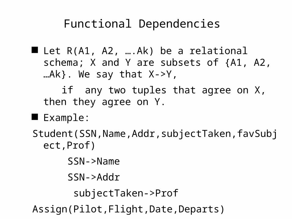
Let R(A1, A2, ….Ak) be a relational schema; X and Y are subsets of {A1, A2, …Ak}. We say that X->Y,
if any two tuples that agree on X, then they agree on Y.
Example:
Student(SSN,Name,Addr,subjectTaken,favSubject,Prof)
SSN->Name
SSN->Addr
subjectTaken->Prof
Assign(Pilot,Flight,Date,Departs)
Pilot,Date,Departs->Flight
Flight,Date->Pilot
Functional Dependencies
• A functional dependency X->Y is trivial if it is satisfied by any relation that includes attributes from X and Y
– E.g.
• customer-name, loan-number customer-name
• customer-name customer-name
– In general, is trivial if
Closure of a Set of Functional Dependencies
• Given a set F set of functional dependencies, there are certain other functional dependencies that are logically implied by F.
– E.g. If A B and B C, then we can infer that A C
• The set of all functional dependencies logically implied by F is the closure of F.
• We denote the closure of F by F+.
Closure of a Set of Functional Dependencies
• An inference axiom is a rule that states if a relation satisfies certain FDs, it must also satisfy certain other FDs
• Set of inference rules is sound if the rules lead only to true conclusions
• Set of inference rules is complete, if it can be used to conclude every valid FD on R
• We can find all of F+ by applying Armstrong’s Axioms:– if , then (reflexivity)– if , then (augmentation)– if , and , then (transitivity)
• These rules are – sound and complete
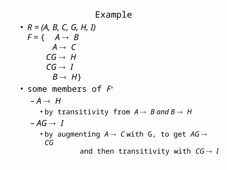
Example
• R = (A, B, C, G, H, I)F = { A B
A CCG HCG I B H}
• some members of F+
– A H • by transitivity from A B and B H
– AG I • by augmenting A C with G, to get AG CG
and then transitivity with CG I
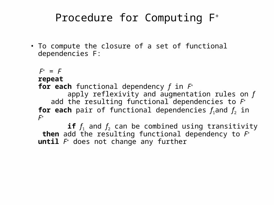
Procedure for Computing F+
• To compute the closure of a set of functional dependencies F:
F+ = Frepeat
for each functional dependency f in F+
apply reflexivity and augmentation rules on f add the resulting functional dependencies to F+
for each pair of functional dependencies f1and f2 in F+
if f1 and f2 can be combined using transitivity then add the resulting functional dependency
to F+
until F+ does not change any further
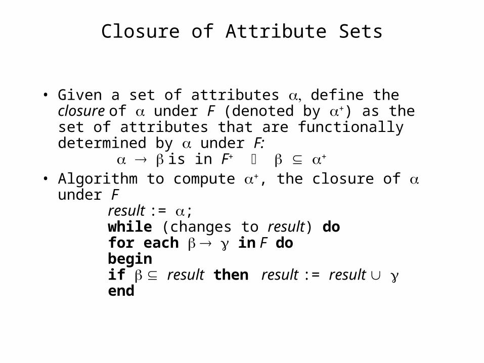
Closure of Attribute Sets
• Given a set of attributes define the closure of under F (denoted by +) as the set of attributes that are functionally determined by under F:
is in F+ +
• Algorithm to compute +, the closure of under Fresult := ;while (changes to result) do
for each in F dobegin
if result then result := result end
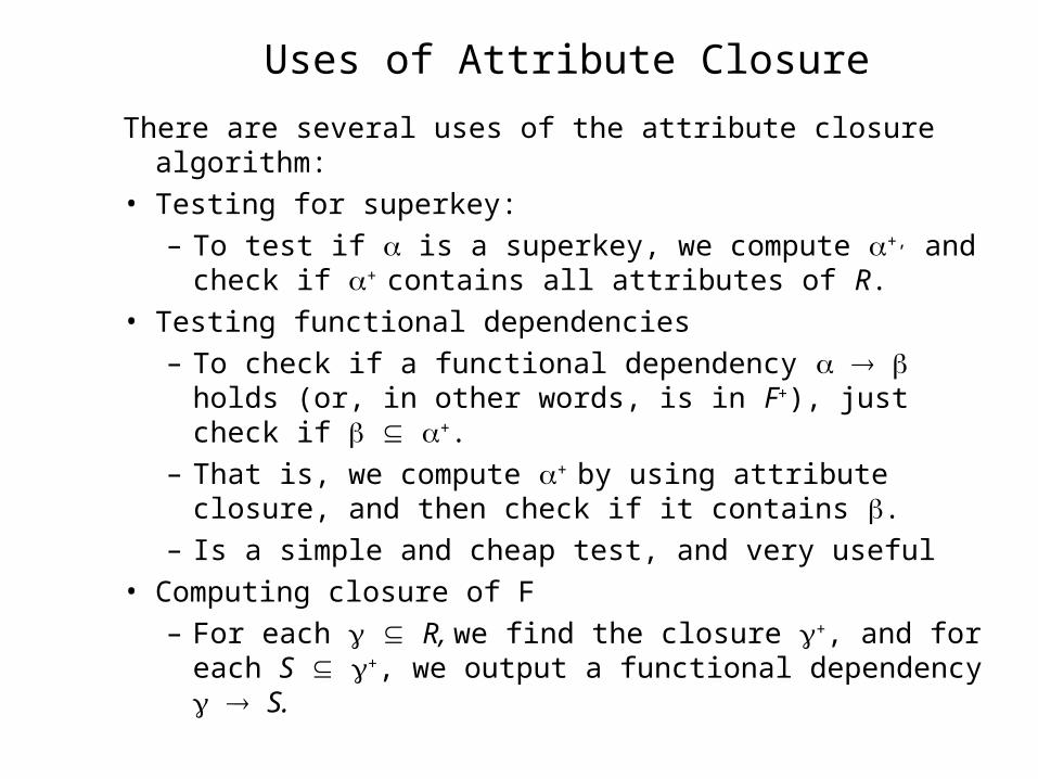
Uses of Attribute Closure
There are several uses of the attribute closure algorithm:
• Testing for superkey:
– To test if is a superkey, we compute +, and check if + contains all attributes of R.
• Testing functional dependencies
– To check if a functional dependency holds (or, in other words, is in F+), just check if +.
– That is, we compute + by using attribute closure, and then check if it contains .
– Is a simple and cheap test, and very useful
• Computing closure of F
– For each R, we find the closure +, and for each S +, we output a functional dependency S.
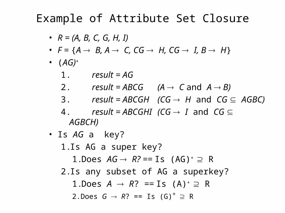
Example of Attribute Set Closure
• R = (A, B, C, G, H, I)
• F = {A B, A C, CG H, CG I, B H}
• (AG)+
1. result = AG
2. result = ABCG (A C and A B)
3. result = ABCGH (CG H and CG AGBC)
4. result = ABCGHI (CG I and CG AGBCH)
• Is AG a key?
1. Is AG a super key?
1. Does AG R? == Is (AG)+ R
2. Is any subset of AG a superkey?
1. Does A R? == Is (A)+ R
2. Does G R? == Is (G)+ R
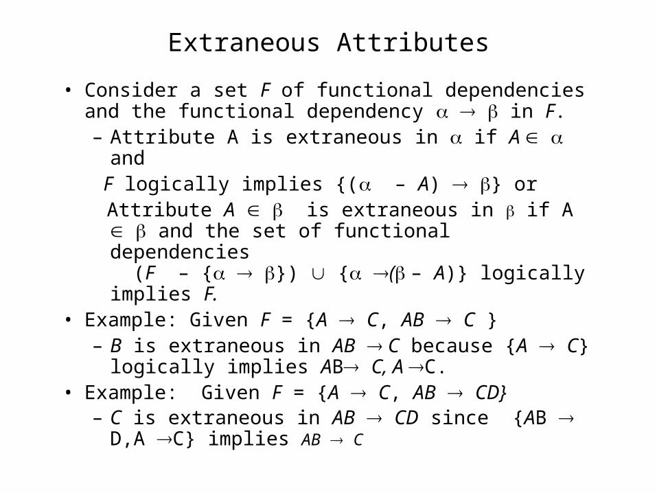
Extraneous Attributes
• Consider a set F of functional dependencies and the functional dependency in F.– Attribute A is extraneous in if A and F logically implies {( – A) } or Attribute A is extraneous in if A and the set
of functional dependencies (F – { }) { ( – A)} logically implies F.
• Example: Given F = {A C, AB C }– B is extraneous in AB C because {A C} logically
implies AB C, A C.• Example: Given F = {A C, AB CD}
– C is extraneous in AB CD since {AB D,A C} implies AB C
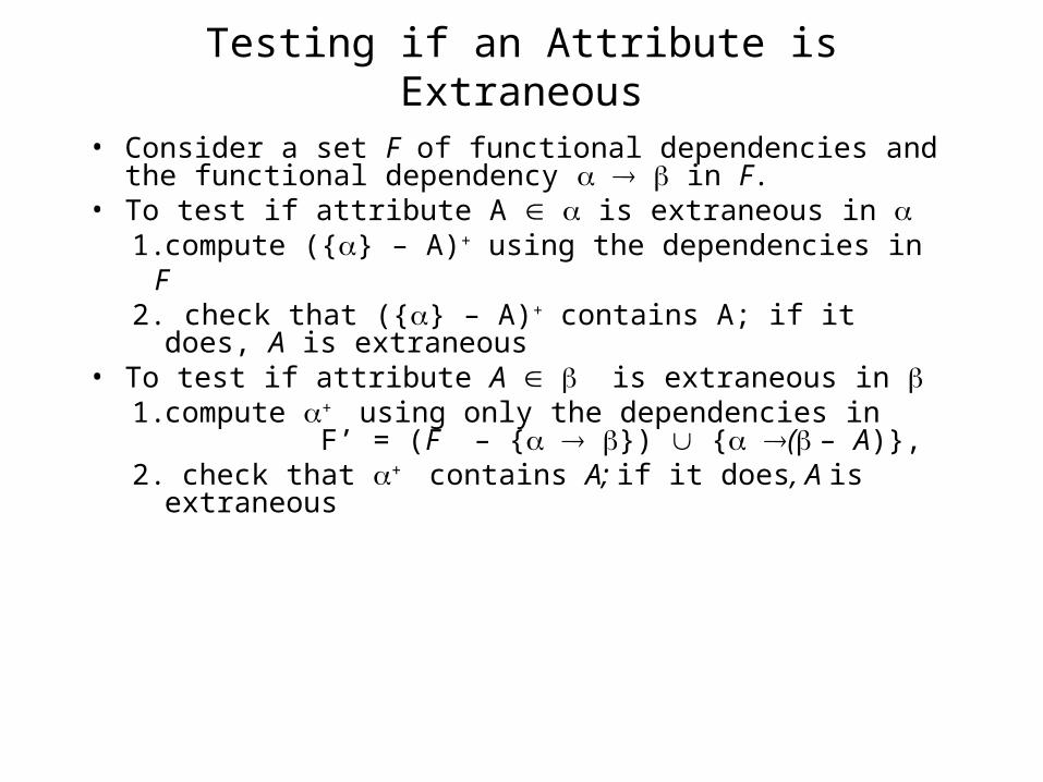
Testing if an Attribute is Extraneous
• Consider a set F of functional dependencies and the functional dependency in F.
• To test if attribute A is extraneous in 1. compute ({} – A)+ using the dependencies in F2. check that ({} – A)+ contains A; if it does, A is
extraneous• To test if attribute A is extraneous in
1. compute + using only the dependencies in F’ = (F – { }) { ( – A)},
2. check that + contains A; if it does, A is extraneous
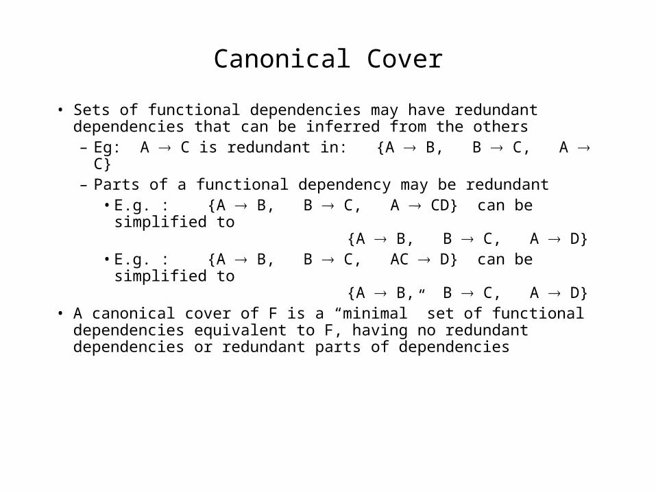
Canonical Cover
• Sets of functional dependencies may have redundant dependencies that can be inferred from the others– Eg: A C is redundant in: {A B, B C, A C}– Parts of a functional dependency may be redundant
• E.g. : {A B, B C, A CD} can be simplified to {A B, B C, A D}
• E.g. : {A B, B C, AC D} can be simplified to {A B, B C, A D}
• A canonical cover of F is a “minimal” set of functional dependencies equivalent to F, having no redundant dependencies or redundant parts of dependencies
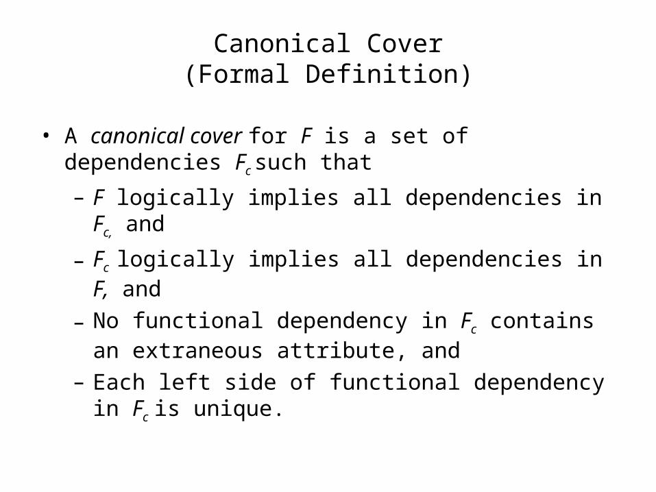
Canonical Cover(Formal Definition)
• A canonical cover for F is a set of dependencies Fc such that
– F logically implies all dependencies in Fc, and
– Fc logically implies all dependencies in F, and
– No functional dependency in Fc contains an extraneous attribute, and
– Each left side of functional dependency in Fc is unique.
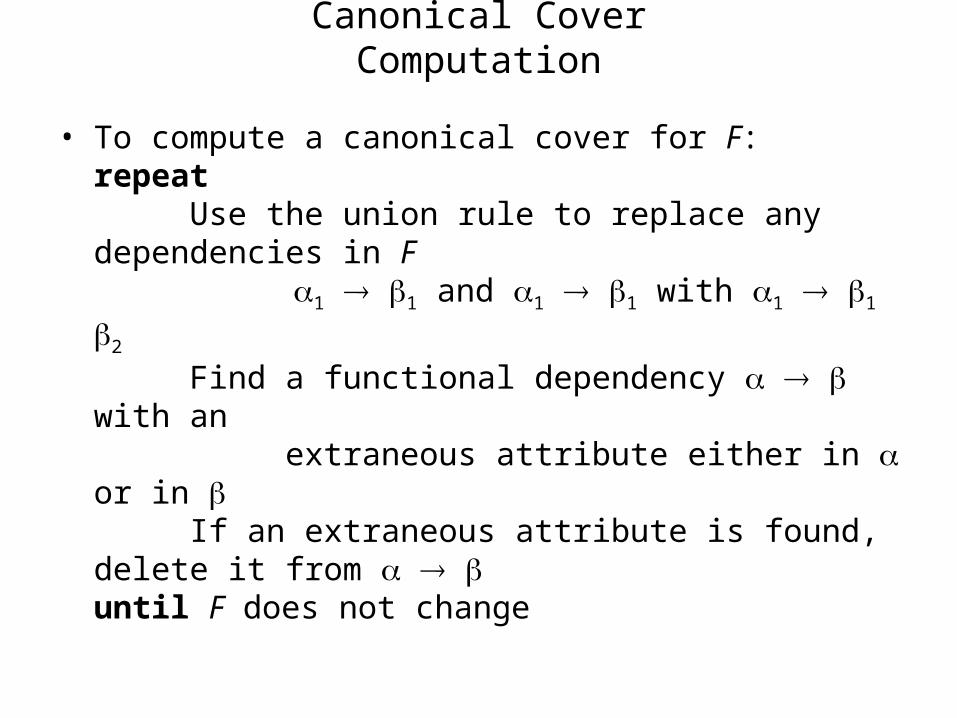
Canonical CoverComputation
• To compute a canonical cover for F:repeat
Use the union rule to replace any dependencies in F 1 1 and 1 1 with 1 1 2
Find a functional dependency with an extraneous attribute either in or in
If an extraneous attribute is found, delete it from
until F does not change
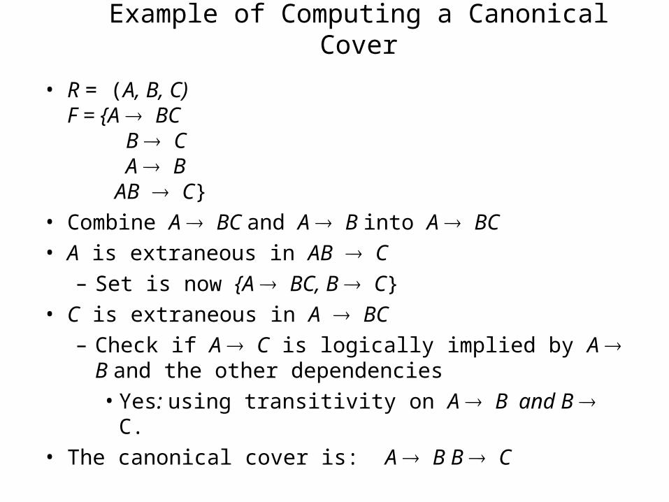
Example of Computing a Canonical Cover
• R = (A, B, C)F = {A BC
B C A BAB C}
• Combine A BC and A B into A BC
• A is extraneous in AB C
– Set is now {A BC, B C}
• C is extraneous in A BC
– Check if A C is logically implied by A B and the other dependencies
• Yes: using transitivity on A B and B C.
• The canonical cover is: A B B C
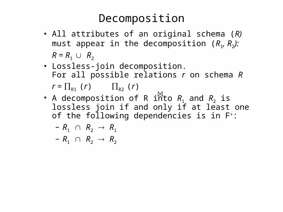
Decomposition• All attributes of an original schema (R) must appear in the
decomposition (R1, R2):
R = R1 R2
• Lossless-join decomposition.For all possible relations r on schema R
r = R1 (r) R2 (r) • A decomposition of R into R1 and R2 is lossless join if and
only if at least one of the following dependencies is in F+:– R1 R2 R1
– R1 R2 R2

Normalization Using Functional Dependencies
• When we decompose a relation schema R with a set of functional dependencies F into R1, R2,.., Rn we want
– Lossless-join decomposition: Otherwise decomposition would result in information loss.
– Dependency preservation: Let Fi be the set of dependencies F+ that include only attributes in Ri.
(F1 F2 … Fn)+ = F+
.
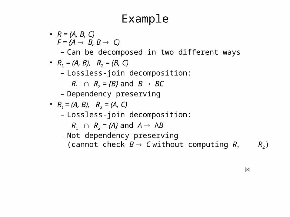
Example• R = (A, B, C)
F = {A B, B C)– Can be decomposed in two different ways
• R1 = (A, B), R2 = (B, C)– Lossless-join decomposition:
R1 R2 = {B} and B BC– Dependency preserving
• R1 = (A, B), R2 = (A, C)– Lossless-join decomposition:
R1 R2 = {A} and A AB– Not dependency preserving
(cannot check B C without computing R1 R2)
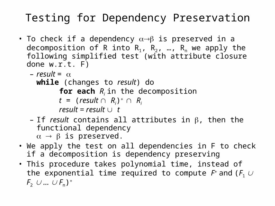
Testing for Dependency Preservation
• To check if a dependency is preserved in a decomposition of R into R1, R2, …, Rn we apply the following simplified test (with attribute closure done w.r.t. F)– result =
while (changes to result) dofor each Ri in the decomposition
t = (result Ri)+ Ri
result = result t– If result contains all attributes in , then the functional
dependency is preserved.
• We apply the test on all dependencies in F to check if a decomposition is dependency preserving
• This procedure takes polynomial time, instead of the exponential time required to compute F+ and (F1 F2 … Fn)+
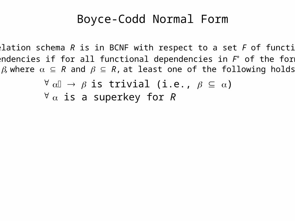
Boyce-Codd Normal Form
is trivial (i.e., ) is a superkey for R
A relation schema R is in BCNF with respect to a set F of functional
dependencies if for all functional dependencies in F+ of the form , where R and R, at least one of the following holds:
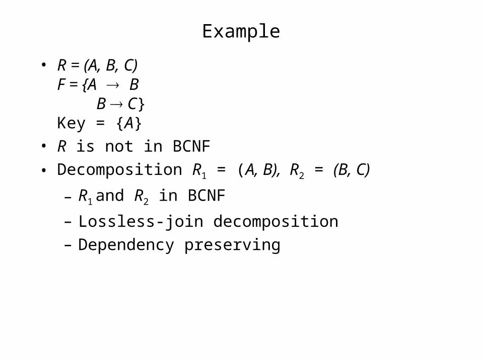
Example
• R = (A, B, C)F = {A B
B C}Key = {A}
• R is not in BCNF
• Decomposition R1 = (A, B), R2 = (B, C)
– R1 and R2 in BCNF
– Lossless-join decomposition
– Dependency preserving
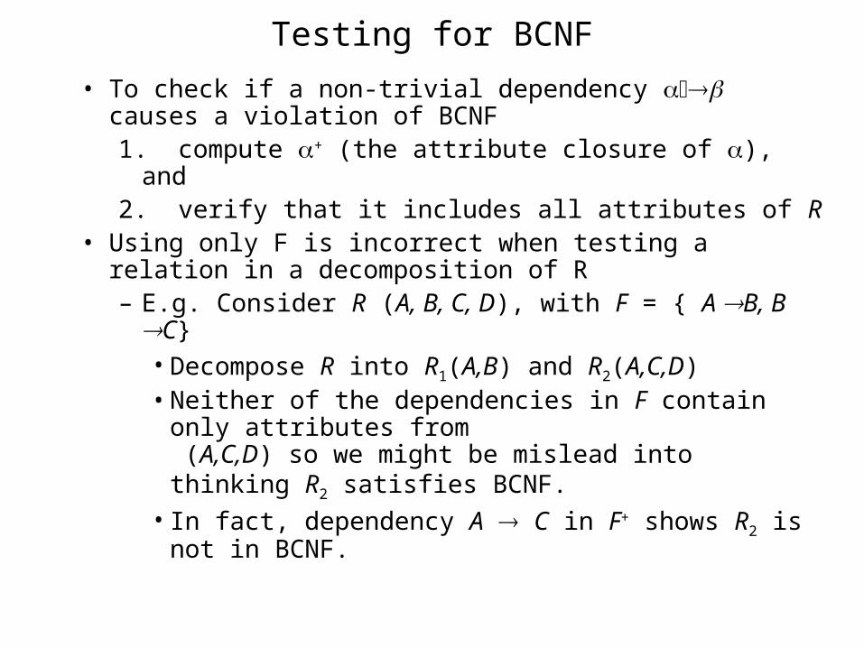
Testing for BCNF
• To check if a non-trivial dependency causes a violation of BCNF1. compute + (the attribute closure of ), and 2. verify that it includes all attributes of R
• Using only F is incorrect when testing a relation in a decomposition of R– E.g. Consider R (A, B, C, D), with F = { A B, B C}
• Decompose R into R1(A,B) and R2(A,C,D) • Neither of the dependencies in F contain only
attributes from (A,C,D) so we might be mislead into thinking R2 satisfies BCNF.
• In fact, dependency A C in F+ shows R2 is not in BCNF.
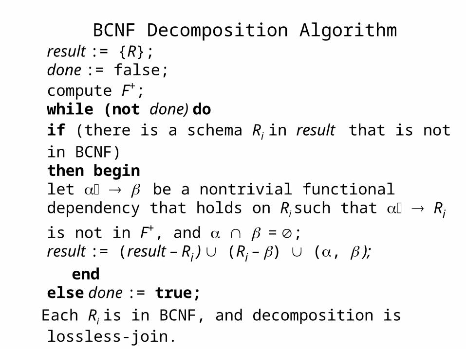
BCNF Decomposition Algorithmresult := {R};done := false;compute F+;while (not done) do
if (there is a schema Ri in result that is not in BCNF)
then beginlet be a nontrivial functional
dependency that holds on Ri such that Ri is not in
F+, and = ;result := (result – Ri ) (Ri – ) (, );
endelse done := true;
Each Ri is in BCNF, and decomposition is lossless-join.
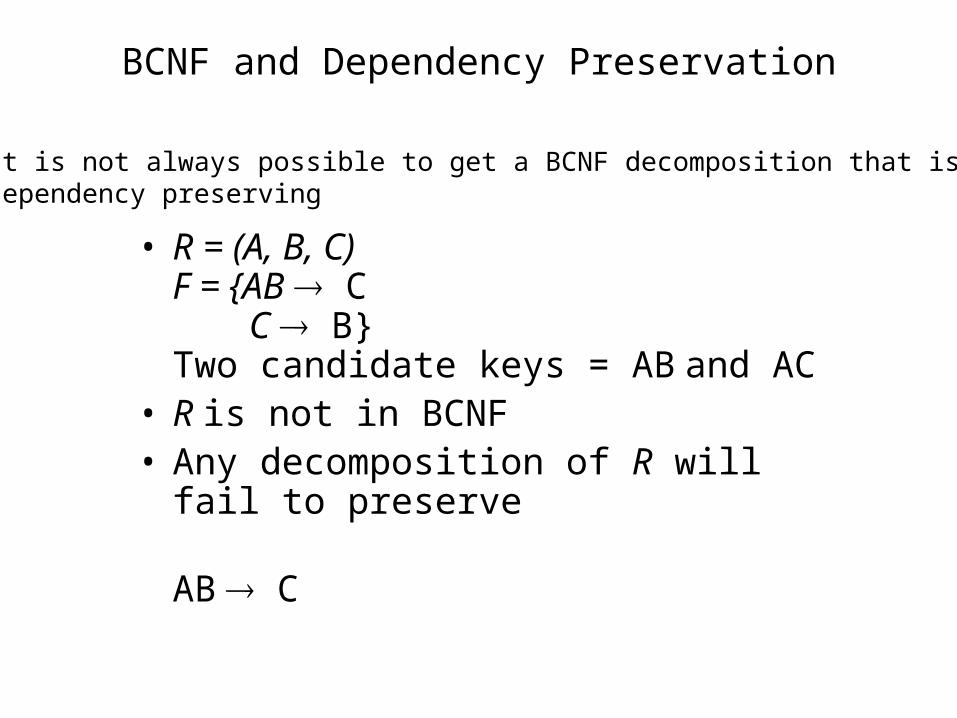
BCNF and Dependency Preservation
• R = (A, B, C)F = {AB C
C B}Two candidate keys = AB and AC
• R is not in BCNF• Any decomposition of R will fail to
preserve
AB C
It is not always possible to get a BCNF decomposition that is dependency preserving
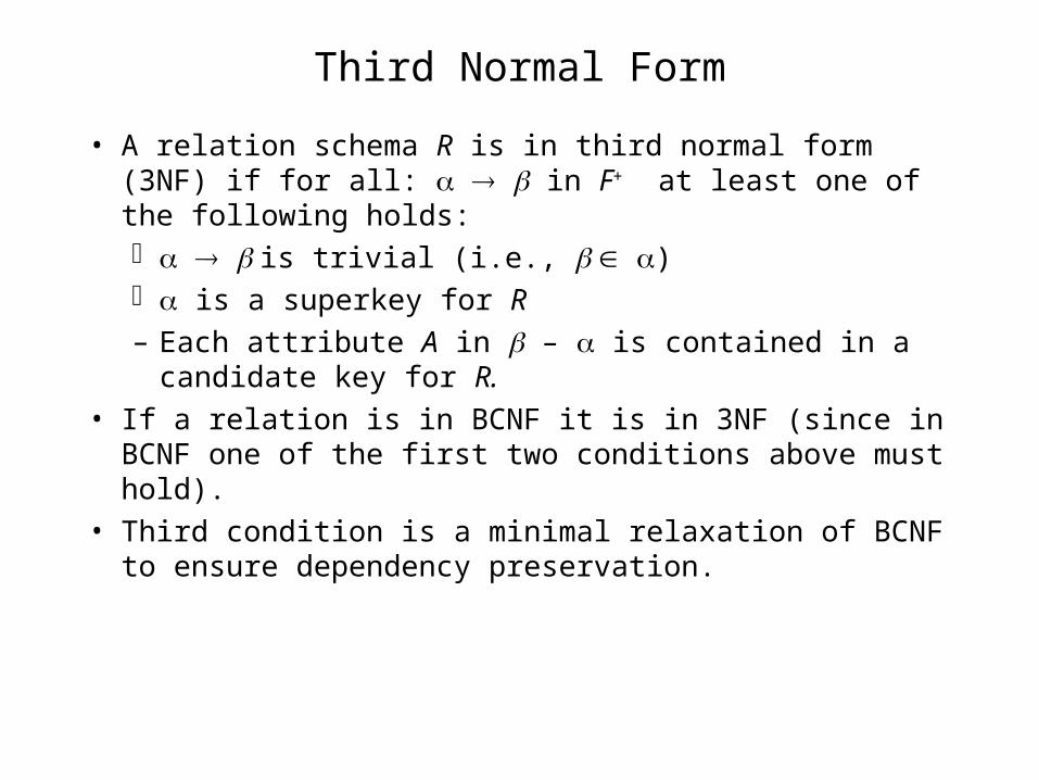
Third Normal Form
• A relation schema R is in third normal form (3NF) if for all: in F+ at least one of the following holds: is trivial (i.e., ) is a superkey for R
– Each attribute A in – is contained in a candidate key for R.
• If a relation is in BCNF it is in 3NF (since in BCNF one of the first two conditions above must hold).
• Third condition is a minimal relaxation of BCNF to ensure dependency preservation.
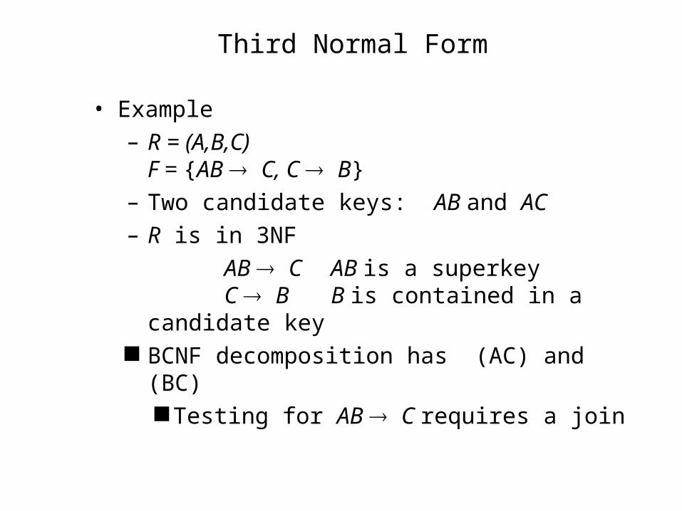
Third Normal Form
• Example
– R = (A,B,C)F = {AB C, C B}
– Two candidate keys: AB and AC
– R is in 3NF
AB C AB is a superkeyC B B is contained in a candidate key
BCNF decomposition has (AC) and (BC) Testing for AB C requires a join
Testing for 3NF
• Use attribute closure to check for each dependency , if is a superkey.
• If is not a superkey, we have to verify if each attribute in is contained in a candidate key of R
– this test is rather more expensive, since it involve finding candidate keys
– testing for 3NF has been shown to be NP-hard
– However, decomposition into third normal form can be done in polynomial time
3NF Decomposition Algorithm
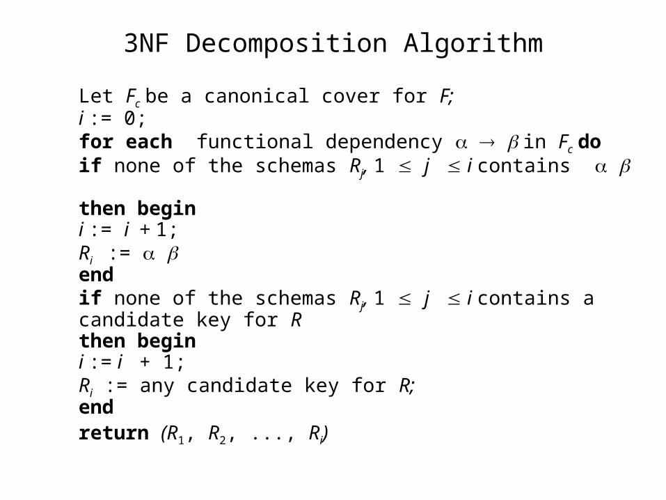
Let Fc be a canonical cover for F;i := 0;for each functional dependency in Fc do
if none of the schemas Rj, 1 j i contains then begini := i + 1;Ri := end
if none of the schemas Rj, 1 j i contains a candidate key for R
then begini := i + 1;Ri := any candidate key for R;end
return (R1, R2, ..., Ri)
Storage Hierarchy
Storage Hierarchy
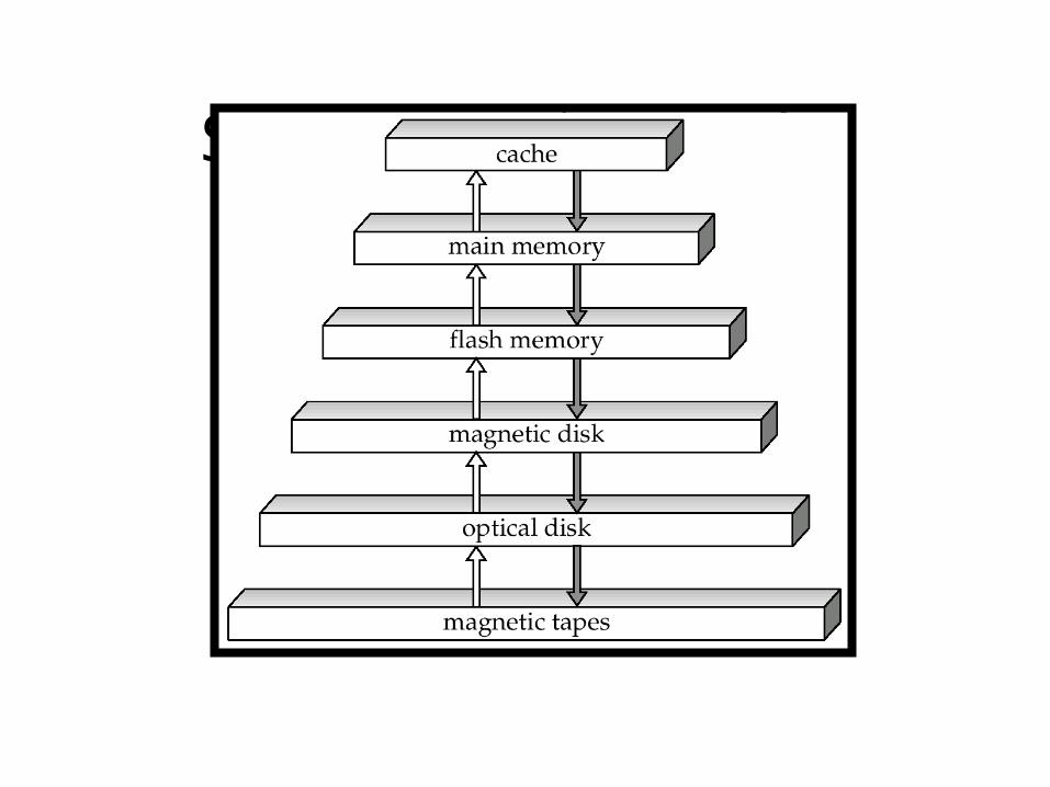
• primary storage: Fastest media but volatile (cache, main memory).
• secondary storage: next level in hierarchy, non-volatile, moderately fast access time
– also called on-line storage
– E.g. flash memory, magnetic disks
• tertiary storage: lowest level in hierarchy, non-volatile, slow access time
– also called off-line storage
– E.g. magnetic tape, optical storage
Magnetic Disks• Disk controller – interfaces between the computer system
and the disk drive hardware.– accepts high-level commands to read or write a sector – initiates actions such as moving the disk arm to the right
track and actually reading or writing the data– Computes and attaches checksums to each sector to
verify that data is read back correctly• If data is corrupted, with very high probability stored
checksum won’t match recomputed checksum– Ensures successful writing by reading back sector after
writing it– Performs remapping of bad sectors
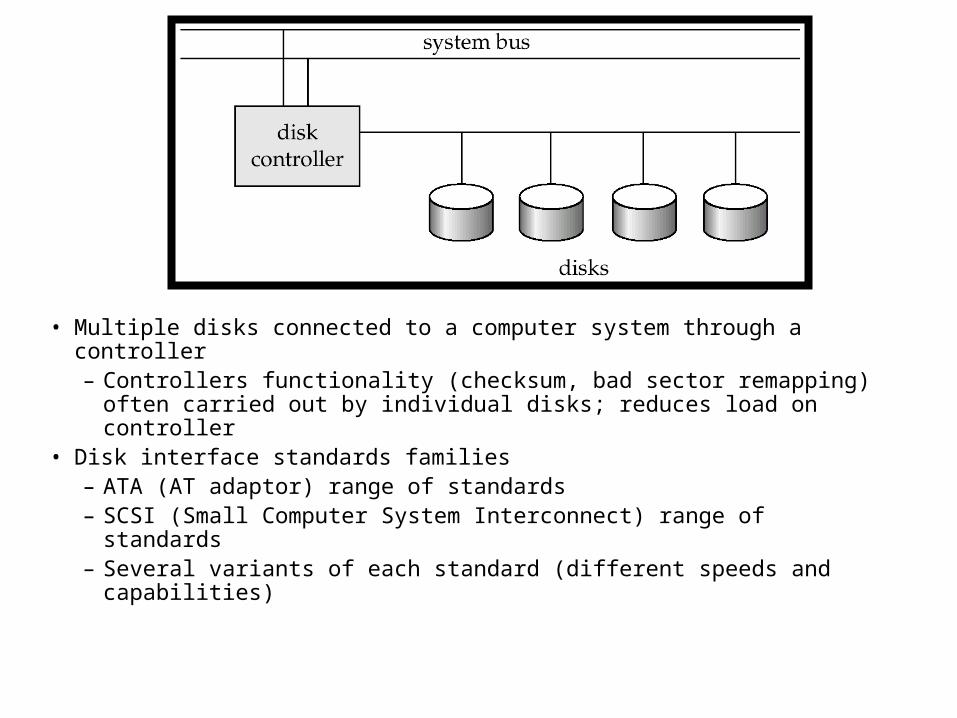
Disk Subsystem
• Multiple disks connected to a computer system through a controller– Controllers functionality (checksum, bad sector remapping)
often carried out by individual disks; reduces load on controller• Disk interface standards families
– ATA (AT adaptor) range of standards – SCSI (Small Computer System Interconnect) range of standards– Several variants of each standard (different speeds and
capabilities)
Performance Measures of Disks• Access time – the time it takes from when a read or write request is
issued to when data transfer begins. Consists of: – Seek time – time it takes to reposition the arm over the correct
track. • Average seek time is 1/2 the worst case seek time.• 4 to 10 milliseconds on typical disks
– Rotational latency – time it takes for the sector to be accessed to appear under the head. • Average latency is 1/2 of the worst case latency.• 4 to 11 milliseconds on typical disks
– Data-transfer rate – the rate at which data can be retrieved from or stored to the disk. • 4 to 8 MB per second is typical
– Multiple disks may share a controller, so transfer rate that controller can handle is also important• E.g. ATA-5: 66 MB/second, SCSI-3: 40 MB/s• Fiber Channel: 256 MB/s
Storage Access
• A database file is partitioned into fixed-length storage units called blocks. Blocks are units of both storage allocation and data transfer.
• Database system seeks to minimize the number of block transfers between the disk and memory. We can reduce the number of disk accesses by keeping as many blocks as possible in main memory.
• Buffer – portion of main memory available to store copies of disk blocks.
• Buffer manager – subsystem responsible for allocating buffer space in main memory.
Buffer Manager• Programs call on the buffer manager when they need a block
from disk.
1. If the block is already in the buffer, the requesting program is given the address of the block in main memory
2. If the block is not in the buffer,
1. the buffer manager allocates space in the buffer for the block, replacing (throwing out) some other block, if required, to make space for the new block.
2. The block that is thrown out is written back to disk only if it was modified since the most recent time that it was written to/fetched from the disk.
3. Once space is allocated in the buffer, the buffer manager reads the block from the disk to the buffer, and passes the address of the block in main memory to requester.
Buffer-Replacement Policies
• Most operating systems replace the block least recently used (LRU strategy)
• Idea behind LRU – use past pattern of block references as a predictor of future references
• Queries have well-defined access patterns (such as sequential scans), and a database system can use the information in a user’s query to predict future references– LRU can be a bad strategy for certain access patterns involving
repeated scans of data• e.g. when computing the join of 2 relations r and s by a nested
loops for each tuple tr of r do for each tuple ts of s do if the tuples tr and ts match …
– Mixed strategy with hints on replacement strategy providedby the query optimizer is preferable
Buffer-Replacement Policies• Pinned block – memory block that is not allowed to be
written back to disk.• Toss-immediate strategy – frees the space occupied by a
block as soon as the final tuple of that block has been processed
• Most recently used (MRU) strategy – system must pin the block currently being processed. After the final tuple of that block has been processed, the block is unpinned, and it becomes the most recently used block.
• Buffer manager can use statistical information regarding the probability that a request will reference a particular relation– E.g., the data dictionary is frequently accessed. Heuristic:
keep data-dictionary blocks in main memory buffer• Buffer managers also support forced output of blocks for the
purpose of recovery
File Organization
• The database is stored as a collection of files. Each file is a sequence of records. A record is a sequence of fields.
• One approach:
– assume record size is fixed
– each file has records of one particular type only
– different files are used for different relations
This case is easiest to implement; will consider variable length records later.
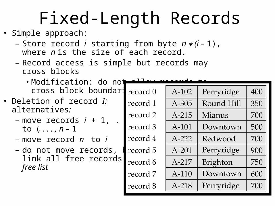
Fixed-Length Records• Simple approach:
– Store record i starting from byte n (i – 1), where n is the size of each record.
– Record access is simple but records may cross blocks• Modification: do not allow records to cross block
boundaries• Deletion of record I:
alternatives:– move records i + 1, . . ., n
to i, . . . , n – 1– move record n to i– do not move records, but
link all free records on afree list
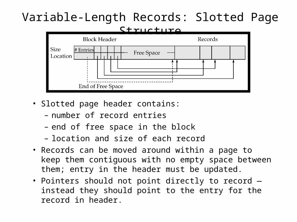
Variable-Length Records: Slotted Page Structure
• Slotted page header contains:
– number of record entries
– end of free space in the block
– location and size of each record
• Records can be moved around within a page to keep them contiguous with no empty space between them; entry in the header must be updated.
• Pointers should not point directly to record — instead they should point to the entry for the record in header.
Organization of Records in Files
• Heap – a record can be placed anywhere in the file where there is space
• Sequential – store records in sequential order, based on the value of the search key of each record
• Hashing – a hash function computed on some attribute of each record; the result specifies in which block of the file the record should be placed
• Records of each relation may be stored in a separate file. In a clustering file organization records of several different relations can be stored in the same file
– Motivation: store related records on the same block to minimize I/O
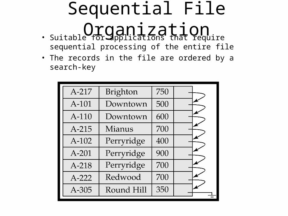
Sequential File Organization• Suitable for applications that require sequential
processing of the entire file
• The records in the file are ordered by a search-key
Clustering File Organization• Simple file structure stores each relation in a separate file • Can instead store several relations in one file using a clustering file organization• E.g., clustering organization of customer and depositor:
• l scan using a secondary index is expensive – each record access may fetch a new block from disk
• an entry was deleted from their parent)• Root node then had only one child, and was deleted and its child became the new root node