Embed Size (px)
Citation preview

Data Structuresand
Algorithms
Course slides: Hashing
www.mif.vu.lt/~algis
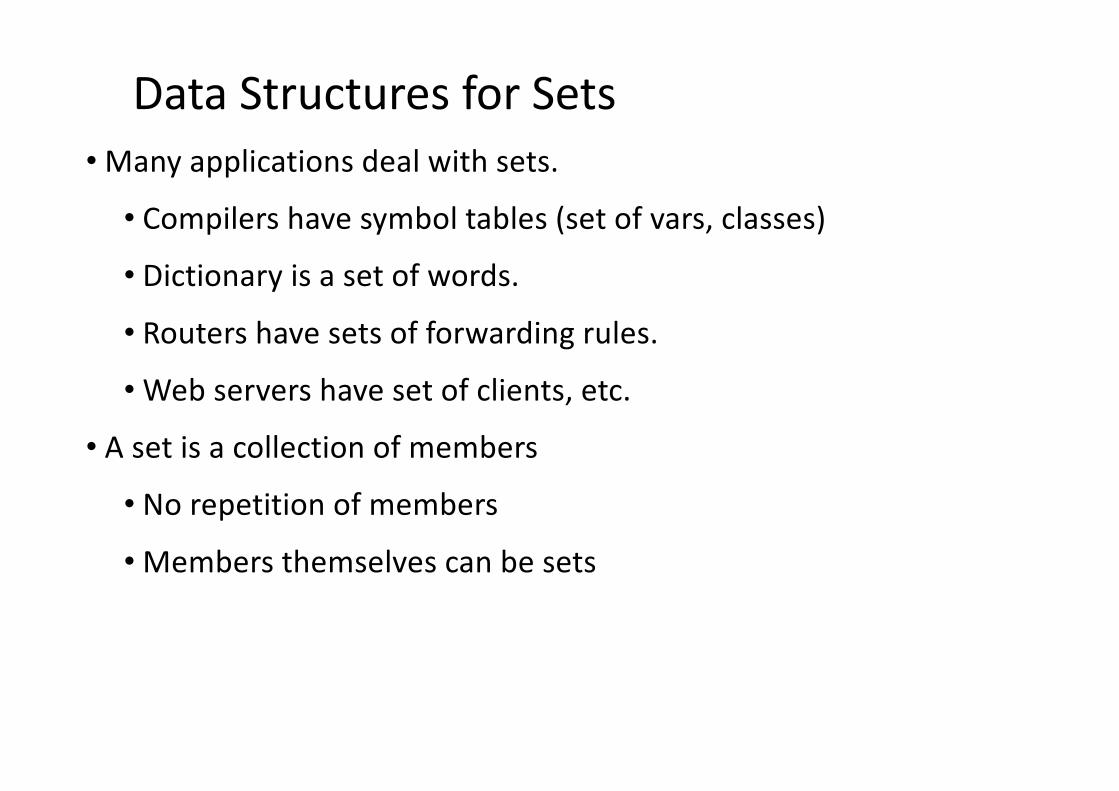
Data Structures for Sets• Many applications deal with sets.
• Compilers have symbol tables (set of vars, classes)
• Dictionary is a set of words.
• Routers have sets of forwarding rules.
• Web servers have set of clients, etc.
• A set is a collection of members
• No repetition of members
• Members themselves can be sets

Set Operations
• Unary operation: min, max, sort, makenull, …
Binary operations
Member Set
Member Order (=, <, >)
Find, insert, delete, split, …
Set Find, insert, delete, split, …
Union, intersection, difference, equal, …
Observations
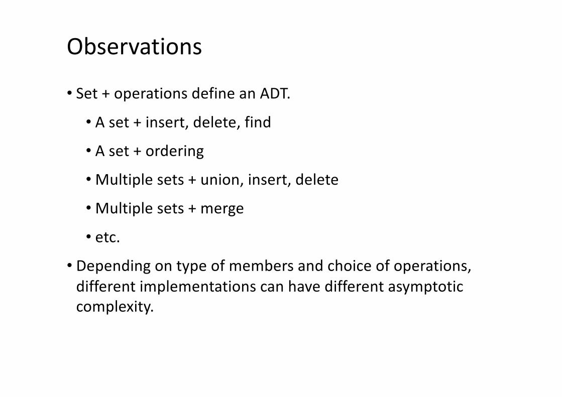
• Set + operations define an ADT.
• A set + insert, delete, find
• A set + ordering
• Multiple sets + union, insert, delete
• Multiple sets + merge
• etc.
• Depending on type of members and choice of operations, different implementations can have different asymptotic complexity.
Dictionary ADTs• Maintain a set of items with distinct keys with:
• find (k): find item with key k
• insert (x): insert item x into the dictionary
• remove (k): delete item with key k
• Where do we use them:
• Symbol tables for compiler
• Customer records (access by name)
• Games (positions, configurations)
• Spell checkers
• Peer to Peer systems (access songs by name), etc.
Naïve Implementations• The simplest possible scheme to implement a dictionary is “log
file” or “audit trail”.• Maintain the elements in a linked list, with insertions occuring
at the head.
• The search and delete operations require searching the entire list in the worst-case.
• Insertion is O (1), but find and delete are O (n).
• A sorted array does not help, even with ordered keys.
• The search becomes fast, but insert/delete take O(n).

Hash Tables: Intuition• Hashing is function that maps each key to a location in memory.
• A keyʼs location does not depend on other elements, and does not change after insertion.
• unlike a sorted list
• A good hash function should be easy to compute.
• With such a hash function, the dictionary operations can be implemented in O (1) time.

Hash Tables: Intuition• Let us denote the set of all possible key values (i.e., the universe
of keys) used in a dictionary application by U.
• An application may require a dictionary in which elements are assigned keys from the set of small natural numbers.
• That is, U ⊂ Z+ and ⏐U⏐ is relatively small.
• If no two elements have same key, this dictionary can be implemented by storing its elements in array T[0, ... , ⏐U⏐ - 1].
• This implementation is referred to as a direct-access table since each of the requisite DICTIONARY ADT operations - Search, Insert, and Delete - can always be performed in Θ(1) time by using a given key value to index directly into T

Hash Tables: Intuition
• The obvious shortcoming associated with direct-access tables is that the set U rarely has such "nice" properties.
• In practice, ⏐U⏐ can be quite large.
• This will lead to wasted memory if the number of elements actually stored in the table is small relative to ⏐U⏐.
• Furthermore, it may be difficult to ensure that all keys are unique.
• Finally, a specific application may require that the key values be real numbers, or some symbols which cannot be used directly to index into the table.
Hash Tables: Intuition• An effective alternative to direct-access tables are hash tables.
• A hash table is a sequentially mapped data structure
• It is similar to a direct-access table in that both attempt to make use of the random- access capability afforded by sequential mapping.

Hash Tables: Intuition
Hashing
Hashing Procedures Let us denote the set of all possible key values (i.e., the universe of keys) used in a dictionary application by U. Suppose an application requires a dictionary in which elements are assigned keys from the set of small natural numbers. That is, U � Z+ and ~U~ is relatively small. If no two elements have the same key, then this dictionary can be implemented by storing its elements in the array T[0, … , ~U~ - 1]. This implementation is referred to as a direct-access table since each of the requisite DICTIONARY ADT operations - Search, Insert, and Delete - can always be performed in 4(1) time by using a given key value to index directly into T, as shown:
The obvious shortcoming associated with direct-access tables is that the set U rarely has such "nice" properties. In practice, ~U~ can be quite large. This will lead to wasted memory if the number of elements actually stored in the table is small relative to ~U~. Furthermore, it may be difficult to ensure that all keys are unique. Finally, a specific application may require that the key values be real numbers, or some symbols which cannot be used directly to index into the table. An effective alternative to direct-access tables are hash tables. A hash table is a sequentially mapped data structure that is similar to a direct-access table in that both attempt to make use of the random-access capability afforded by sequential mapping. However, instead of using a key value to directly index into the hash table, the index is computed from the key value using a hash function, which we will denote using h. This situation is depicted as follows:
Hash Tables• All search structures so far
• Relied on a comparison operation
• Performance O (n) or O (log n)
• Assume there is a function
• f ( key ) → { integer value }
i.e. a function that maps a key to an integer
• What performance might I expect now?
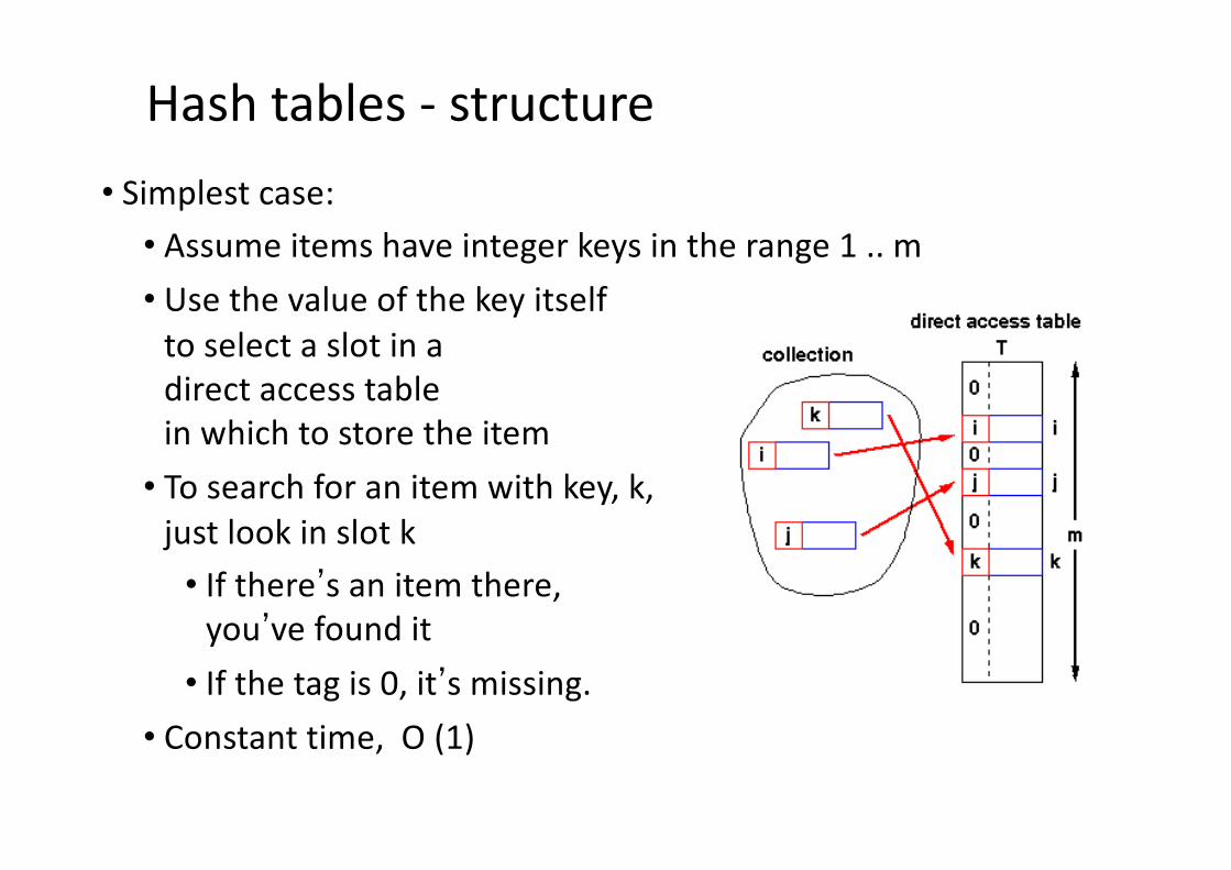
Hash tables - structure• Simplest case:
• Assume items have integer keys in the range 1 .. m• Use the value of the key itself
to select a slot in a direct access table in which to store the item
• To search for an item with key, k,just look in slot k
• If thereʼs an item there,youʼve found it
• If the tag is 0, itʼs missing.• Constant time, O (1)

Hashing : the basic idea
• Map key values to hash table addresses
keys -> hash table address
This applies to find, insert, and remove
• Usually: integers -> {0, 1, 2, …, Hsize-1}
• Typical example: f (n) = n mod Hsize
• Non-numeric keys converted to numbers
• For example, strings converted to numbers as
• Sum of ASCII values
• First three characters
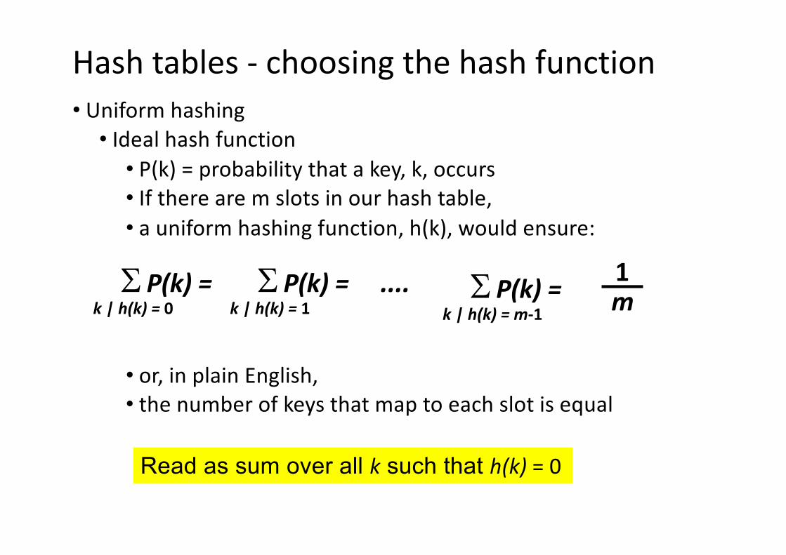
Hash tables - choosing the hash function• Uniform hashing
• Ideal hash function• P(k) = probability that a key, k, occurs• If there are m slots in our hash table,• a uniform hashing function, h(k), would ensure:
• or, in plain English, • the number of keys that map to each slot is equal
SP(k) =k | h(k) = 0
SP(k) = ....k | h(k) = 1
SP(k) =k | h(k) = m-1
1m
Read as sum over all k such that h(k) = 0

Hash Tables - A Uniform Hash Function• If the keys are integers randomly distributed in [ 0 , r ), then
is a uniform hash function.• Most hashing functions can be made to map the keys to [ 0 , r )
for some r• For example, adding the ASCII codes for characters mod 255 will
give values in [ 0, 256 ) or [ 0, 255 ]• Replace + by xor same range without the mod operation
Read as 0 ≤ k < rh(k) = mk
r

Hash Tables - Reducing the range to [ 0, m )• Weʼve mapped the keys to a range of integers
0 =< k < r
• Now we must reduce this range to [ 0, m )
where m is a reasonable size for the hash table
• Strategies:
• Division - use a mod function
• Multiplication
• Universal hashing

Hash Tables - Reducing the range to [ 0, m )Division
• Use a mod function
h (k) = k mod m
• Choice of m ?
• Powers of 2 are generally not good!h(k) = k mod 2n
selects last n bits of k
• All combinations are not generally equally likely
• Prime numbers close to 2 n seem to be good choices
eg want ~4000 entry table, choose m = 4093
0110010111000011010
k mod 28 selects these bits

Hash Tables - Reducing the range to [0, m )Multiplication method
• Multiply the key k by constant, A, 0 < A < 1
• Extract the fractional part of the product
k A - ⎣ k A ⎦
• Multiply this by mh(k) = ⎣ m ( k A - ⎣ k A ⎦ ) ⎦
• Now m is not critical and a power of 2 can be chosen.
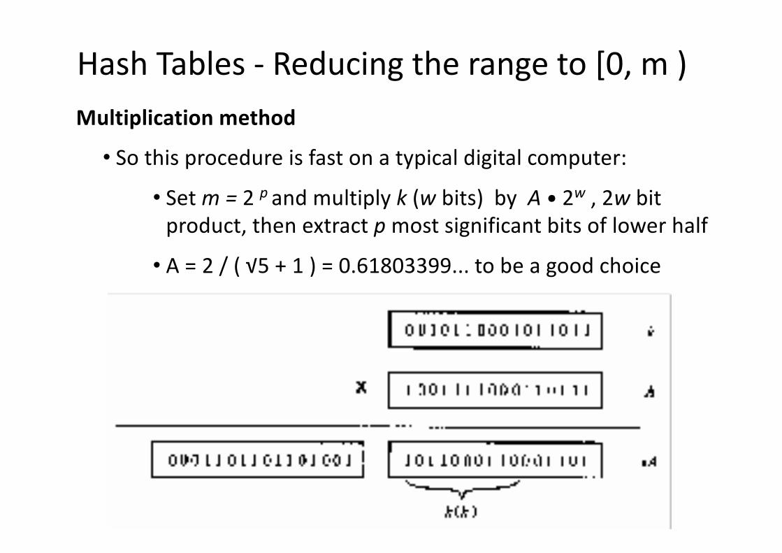
Hash Tables - Reducing the range to [0, m )Multiplication method
• So this procedure is fast on a typical digital computer:
• Set m = 2 p and multiply k (w bits) by A • 2w , 2w bit product, then extract p most significant bits of lower half
• A = 2 / ( √5 + 1 ) = 0.61803399... to be a good choice

Hash Tables - Reducing the range to [0, m)Universal Hashing
Definition: A randomized algorithm H for constructing hash functions
h: U→{1,…,M} is universal if for all x ≠ y in U,
we have Pr [ℎ ( 𝑥 ) = ℎ ( 𝑦 ) ] ≤ 1/𝑀
Select the hash function randomly (at run time) from a set of hash functions to reduce probability of poor performance.
A determined “adversary” can always find a set of data that will defeat any hash function.

Hash Tables - reducing the range to ( 0, m ]Universal Hashing
• We may design a set of universal hash functions easily
• Key, x = x0, x1, x2, ...., xr
• Choose a = <a0, a1, a2, ...., ar> as a sequence of elements chosen randomly from { 0, m-1 }
• ha(x) = Σ aixi mod m
• There are m r+1 sequences a, so there are m r+1 functions, ha(x)

Hash Tables - Constraints• Constraints
• Keys must be unique
• Keys must lie in a small range
• For storage efficiency,keys must be dense in the range
• If theyʼre sparse (lots of gaps between values),a lot of space is used to obtain speed
• Space for speed trade-off

Hash Tables - Relaxing the constraints• Keys must be unique
• Construct a linked list of duplicates “attached” to each slot
• If a search can be satisfiedby any item with key, k,performance is still O(1)but
• If the item has some other distinguishing featurewhich must be matched,we get O(nmax)where nmax is the largest numberof duplicates - or length of the longest chain

Hash Tables - Relaxing the constraints• Keys are integers
• Need a hash functionh ( key ) → integer
Id est: one that maps a key to an integer
• Applying this function to thekey produces an address
• If h maps each key to a uniqueinteger in the range 0 .. m-1then search is O (1)

Hash Tables - Collision handling• Collisions
• Occur when the hash function maps two different keys to the same address
• The table must be able to recognise and resolve this• Recognise
• Store the actual key with the item in the hash table• Compute the address
• k = h ( key )• Check for a hit
• if ( table[k].key == key ) then hitelse try next entry
• Resolution• Variety of techniques

Hash Tables - Separate chaining• 1. Separate chaining
• Collisions - Resolution
Linked list attached to each primary table slot
• h(i) == h(i1)
• h(k) == h(k1) == h(k2)
• Searching for i1
• Calculate h(i1)
• Item in table, i,doesnʼt match
• Follow linked list to i1• If NULL found, key isnʼt in table

Hash tables - Separate chaining• Separate chaining
• Maintain a list of all elements that hash to the same value
• Search -- using the hash function to determine which list to traverse
• Insert/deletion–once the “bucket” is found through Hash, insert and delete are list operations
14
42
29
20
1
36
5623
16
24
31
177
012345678910

Hash tables – Separate chaining
14
42
29
20
1
36
5623
16
24
31
177
012345678910
53 = 4 x 11 + 953 mod 11 = 9
14
42
29
20
1
36
5623
16
24
53
177
012345678910
31
Insertion: insert 53

Analysis of Hashing with Chaining• Worst case
• All keys hash into the same bucket
• a single linked list.
• insert, delete, find take O(n) time.
• Average case
• Keys are uniformly distributed into buckets
• O(1+N/B): N is the number of elements in a hash table, B is the number of buckets.
• If N = O(B), then O(1) time per operation.
• N/B is called the load factor of the hash table.

Hash Tables - Overflow area2. Overflow area
• Linked list constructedin special area of tablecalled overflow area
• h(k) == h(j)• k stored first• Adding j
• Calculate h(j)• Find k• Get first slot in overflow area• Put j in it• kʼs pointer points to this slot
• Searching - same as linked list

Open addressing
• If collision happens, alternative cells are tried until an empty cell is found.
• Linear probing :Try next available position
012345678910
42
9
14
1
16
24
31
287

hʼ(x) -second hash function
Hash Tables - Re-hashing
3. Use a second hash function• Many variations• General term: re-hashing
• H(k) == h(j)• K stored first• Adding j
• Calculate h(j)• Find k• Repeat until we find an empty slot• Calculate hʼ(j)• Put j in it
• Searching – Use h(x), then hʼ(x).

Hash Tables - Re-hash functions4. The re-hash function – Linear probing
• Many variations
• Linear probing
• hʼ(x) is +1
• Go to the next slotuntil you find one empty
• Can lead to bad clustering
• Re-hash keys fill in gapsbetween other keys and exacerbatethe collision problem

Linear Probing (insert 12)
012345678910
42
9
14
1
16
24
31
287
12 = 1 x 11 + 112 mod 11 = 1
012345678910
42
9
14
1
16
24
31
287
12

Search with linear probing (Search 15)
15 = 1 x 11 + 415 mod 11 = 4
012345678910
42
9
14
1
16
24
31
287
12
NOT FOUND !

Deletion with linear probing: LAZY (Delete 9)
9 = 0 x 11 + 99 mod 11 = 9
012345678910
42
9
14
1
16
24
31
287
12
FOUND !
012345678910
42
D
14
1
16
24
31
287
12

remove(j) { i = j;
empty[i] = true;i = (i + 1) % D; // candidate for swappingwhile ((not empty[i]) and i!=j) {
r = Hash(ht[i]); // where should it go without collision?gy?
if not ((j<r<=i) or (i<j<r) or (r<=i<j))then break; // yes find it from rehashing, swapi = (i + 1) % D; // no, cannot find it from
rehashing}if (i!=j and not empty[i])then {
ht[j] = ht[i];remove(i);
}}
Eager Deletion: fill holes!Remove and find replacement:
£Fill in the hole for later searches

Eager Deletion Analysis• If not full
• After deletion, there will be at least two holes• Elements that are affected by the new hole are
• Initial hashed location is cyclically before the new hole
• Location after linear probing is in between the new hole and the next hole in the search order
• Elements are movable to fill the hole
Next hole in the search orderNew hole
Initialhashed location
Location after linear probing
Next hole in the search order
Initialhashed location
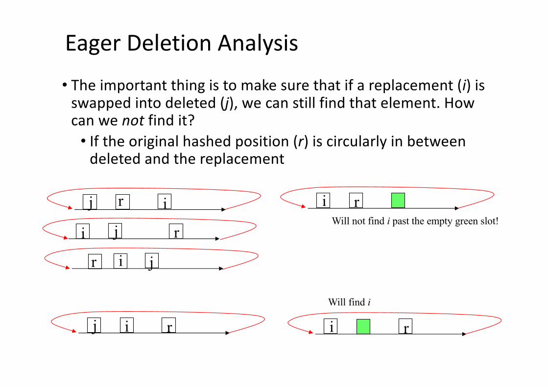
Eager Deletion Analysis
• The important thing is to make sure that if a replacement (i) is swapped into deleted (j), we can still find that element. How can we not find it?
• If the original hashed position (r) is circularly in between deleted and the replacement
j r i
j ri
jr i
i rWill not find i past the empty green slot!
j i r i r
Will find i

Deletion in Hashing with Linear Probing• Since empty buckets are used to terminate search, standard
deletion does not work.
• One simple idea is to not delete, but mark.
• Insert: put item in first empty or marked bucket.
• Search: Continue past marked buckets.
• Delete: just mark the bucket as deleted.
• Advantage: Easy and correct.
• Disadvantage: table can become full with dead items.
41
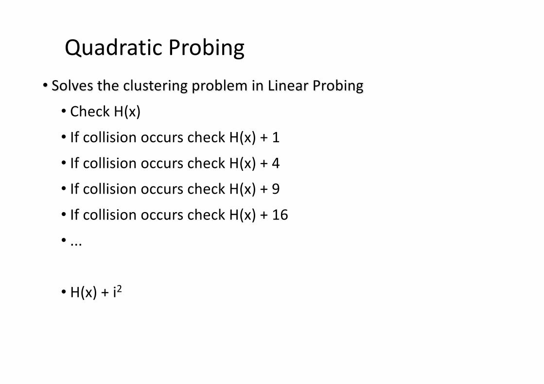
Quadratic Probing• Solves the clustering problem in Linear Probing
• Check H(x)
• If collision occurs check H(x) + 1
• If collision occurs check H(x) + 4
• If collision occurs check H(x) + 9
• If collision occurs check H(x) + 16
• ...
• H(x) + i2

Quadratic Probing (insert 12)
012345678910
42
9
14
1
16
24
31
287
12 = 1 x 11 + 112 mod 11 = 1
012345678910
42
9
14
1
16
24
31
287
12

Double Hashing• When collision occurs use a second hash function
• Hash2 (x) = R – (x mod R)
• R: greatest prime number smaller than table-size
• Inserting 12
H2(x) = 7 – (x mod 7) = 7 – (12 mod 7) = 2
• Check H(x)
• If collision occurs check H(x) + 2
• If collision occurs check H(x) + 4
• If collision occurs check H(x) + 6
• If collision occurs check H(x) + 8
• H(x) + i * H2(x)

Double Hashing (insert 12)
012345678910
42
9
14
1
16
24
31
287
12 = 1 x 11 + 112 mod 11 = 1
7 –12 mod 7 = 2
012345678910
42
9
14
1
16
24
31
287
12

Hash Tables - Re-hash functions5. The re-hash function – Quadratic probing
• Many variations
• Quadratic probing
• hʼ(x) is c i2 on the ith probe
• Avoids primary clustering
• Secondary clustering occurs
• All keys which collide on h(x) follow the same sequence
• First
• a = h (j) = h (k)
• Then a + c, a + 4c, a + 9c, ....
• Secondary clustering generally less of a problem

Hash Tables - Collision Resolution Summary• Chaining
+Unlimited number of elements+Unlimited number of collisions- Overhead of multiple linked lists
• Re-hashing+Fast re-hashing +Fast access through use of main table space- Maximum number of elements must be known- Multiple collisions become probable
• Overflow area+Fast access +Collisions don't use primary table space- Two parameters which govern performance need to be
estimated

Hash Tables - Summary• Potential O(1) search time
• If a suitable function h(key) ® integer can be found• Space for speed trade-off
• “Full” hash tables donʼt work• Collisions
• Inevitable• Hash function reduces amount of information in key
• Various resolution strategies• Linked lists• Overflow areas• Re-hash functions
• Linear probing hʼ is +1• Quadratic probing hʼ is +ci2• Any other hash function!
• or even sequence of functions!

Rehashing• If table gets too full, operations will take too long.
• Build another table, twice as big (and prime).
• Next prime number after 11 x 2 is 23
• Insert every element again to this table
• Rehash after a percentage of the table becomes full (70% for example)
49

Good and Bad Hashing Functions• Hash using the wrong key
• Age of a student
• Hash using limited information
• First letter of last names (a lot of Aʼs, few Zʼs)
• Hash functions choices :
• keys evenly distributed in the hash table
• Even distribution guaranteed by “randomness”• No expectation of outcomes
• Cannot design input patterns to defeat randomness

Examples of Hashing Function• B = 100, N = 100, keys = A0, A1, …, A99
• Hashing (A12) = (Ascii (A) + Ascii (1) + Ascii (2) ) / B
• H (A18) = H (A27) = H (A36) = H (A45) …
• Theoretically, N (1+N/B) = 200
• In reality, 395 steps are needed because of collision
• How to fix it?
• Hashing (A12) = (Ascii (A) * 22 + Ascii (1) * 2 + Ascci (2) ) / B
• H (A12)! = H (A21)
• Examples: numerical keys
• Use X2 and take middle numbers

Hash Tables - Load factor• Collisions are very probable!
• Table load factor must be kept low
• Detailed analyses of the average chain length(or number of comparisons/search) are available
• Separate chaining
• linked lists attached to each slot gives best performance
• but uses more space!
a =n
m
n = number of items
m = number of slots

Hash Tables - General DesignChoose the table size
• Large tables reduce the probability of collisions!• Table size, m• n items• Collision probability a = n / m
Choose a table organisation• Does the collection keep growing?
• Linked lists (....... but consider a tree!)• Size relatively static?
• Overflow area or• Re-hash
Choose a hash function

Hash Tables - General DesignChoose a hash function
• A simple (and fast) one may well be fine ...
• Read your text for some ideas!
Check the hash function against your data
Fixed data
• Try various h, muntil the maximum collision chain is acceptable
"Known performance
Changing data
• Choose some representative data
• Try various h, m until collision chain is OK
"Usually predictable performance

Hash Tables - Review• If you can meet the constraints+ Hash Tables will generally give good performance+ O (1) search
• Like radix sort, they rely on calculating an address from a key
• But, unlike radix sort, relatively easy to get good performance
• with a little experimentation not advisable for unknown data
• collection size relatively static• memory management is actually simpler• All memory is pre-allocated!

Collision Functions• Hi(x)= (H(x)+i) mod B
• Linear pobing
• Hi(x)= (H(x)+ci) mod B (c>1)
• Linear probing with step-size = c
• Hi(x)= (H(x)+i2) mod B
• Quadratic probing
• Hi(x)= (H(x)+ i * H2(x)) mod B
Analysis of Open Hashing• Effort of one Insert?
• Intuitively – that depends on how full the hash is
• Effort of an average Insert?
• Effort to fill the Bucket to a certain capacity?
• Intuitively – accumulated efforts in inserts
• Effort to search an item (both successful and unsuccessful)?
• Effort to delete an item (both successful and unsuccessful)?
• Same effort for successful search and delete?
• Same effort for unsuccessful search and delete?

Picking a Hash Function• In practice, hash functions often use the bit representation of
values.
• e.g. compute the binary representation of the characters in the search key and return the sum modulus the number of buckets.
• e.g. distribute first names over 59 buckets. Use ASCII values of the letters e.g. John (74 + 111 + 104 + 110 = 399), 399 modulo 59 = bucket 45.
• In practice schemes are more complicated than the above. See the big white algorithm book for more details (Cormen, Leiserson, Rivest).
Picking a Hash Function• For a hash table the idea is that there will be n entries.
• n = the number of actual values.
• the hope is that each of the n values maps to a different index (no collisions).
• For DB hash indexing the index is divided into buckets.
• each bucket maps to a disk page (which maps to a disk block).
• The hash function maps index entries to buckets with the intent that no bucket overflows.

Hash Function Problems• Poor distribution of values to buckets.
• This can happen because the hash function is either not random or not uniform.
• Solution: Change the hash function.
• Skewed data distribution.
• The distribution of search key values is skewed.
• That is, there is not a uniform distribution of values –many incidences of some values and few of others.
• Solution: There is no way this can be addressed by changing the hash function.
• If this is a problem then a hash index may not be a good choice.
Hash Function Problems• Collisions
• Overflow may be caused by inserts of data entries with the same hash value (but different search key values).
• Solution:
• Static hashing does not address this.
• Extendible hashing and linear hashing deal with collisions to some extent.

Static Hashing• Hash function
• A uniform and random hash function h evenly maps search key values to a primary page.
• With N buckets the hash function maps a search key value to buckets 0 to N-1.
• Primary pages
• The number of buckets (pages) is pre-determined.
• Each bucket is a disk page.
• Overflow pages
• As the DB grows primary pages become full.
• Additional data is placed in overflow pages chained to the primary pages.
• Finding a value involves searching these pages.

Static Hashing• Performance
• Generally a search requires one disk access.
• Insert or delete require two disk accesses.
• The number of primary pages is fixed.
• The structure becomes inefficient as the file grows (because of the overflow pages).
• It wastes space if the file shrinks.
• Re-hashing removes overflow until the DB grows again. This process is time-consuming and the index is inaccessible during it.

Extendible hashing: uses secondary storage• Suppose data does not fit in main memory
• Goal: Reduce number of disks accesses.
• Suppose N records to store and M records fit in a disk block
• Result: 2 disk accesses for find (~4 for insert)
• Let D be max number of bits so 2^D < M.
• This is for root or directory (a disk block)
• Algo: hash on first D bits, yields ptr to disk block
• Expected number of leaves: (N/M) log 2
• Expected directory size: O (N^ (1+1/M) / M)
• Theoretically difficult, more details for implementation
Extendible Hashing• The efficiency of static hashing declines as the file grows.
• Overflow pages increase search time.
• One solution would be to use a range of hash functions based on a bit value and double the number of buckets (and the function range) whenever an overflow page is needed.
• Such a reorganization is expensive.
• Is it possible to make local changes?

Extendible Hashing• Use a directory of pointers to buckets.
• Double the directory size when required.
• Only split the pages that have overflowed.
• The directory need only consist of an array of pointers to pages so is relatively compact.
• The array index represents the value computed by the hash function.
• At any time the array size is determined by how many bits of the hash result are being used.
• Usually the last d (least significant) bits are used.

Basic Structure
• The array index is the last two bits of the hash value.• Note that the values in the cells represents the hash value (not
the search key value).• Assume that three records fit on a page (so each bucket is a disc
page).• There are only four pages of data and none of the pages is full –
only two bits are required as an index.
64 16
00 1 17 5
01
10
11 6
31 15

Inserting Values
• Insert 14 and 9 into the index shown• 14 fits but inserting 9 causes the page to overflow. • Double the directory and split the overflowing bucket (01)
into two. Distribute the entries based on the last threedigits of the hash value.
• Directory pointers to the existing buckets are added for the other three new three digit hash values.
64 16
00 1 17 5
01 9
10
11 6 14
31 15
insert

Inserting Values Example
• Note how the directory has doubled in size but only one new bucket has been created. The directory is small (each entry consists of a value and a pointer). New index pages (buckets) are kept to a minimum.
64 16
1 17 9
000
001
010 6 14
011
100
101 31 15
110
111
5
new bucket

Keeping Track of Bits• After the directory is doubled some pages will be referenced
by two directory entries.
• If the referenced pages become full, subsequent insertions will require a new page to be allocated but will not require doubling the directory.
• If pages that are referenced by only one directory entry overflow the directory will have to be doubled again.
• Contrast inserting 4 and 12 (x00) into the example with inserting 25 (x01).
Keeping Track of Bits• How do we keep track of whether or not an insert requires
that the directory is doubled?
• Record the global depth of the hashed file.
• The number of bits required for the directory.
• Also record the local depth of each page.
• The number of bits needed to reference a particular page.

Local and Global Depth
2
64 16
3
1 17 9
000
001 2
010 6 14
011
100 2
101 31 15
110
111 3
5
3
local depthglobal depth

Summary• Create initial hash file and directory.
• Each directory entry points to a different bucket.• All local depths are equal to the global depth.
• Insert values• If no overflow occurs insert entry and finish.• If the bucket overflows compare the local depth of the
bucket with the global depth.• If the local depth is less than the global depth create a
new bucket and distribute the entries with no change to the directory. Increment the local depth of the split buckets.

Summary• If the local depth is the same as the global depth double
the directory, and split the bucket.
• Increment the local depth of the split buckets and the global depth of the directory.
• Delete values
• If the deletion empties the bucket it can be merged and the local depth decremented.
• If the local depth of all buckets is less than the global depth the directory can be halved.
• In practice this is often not done
Performance• Performance is identical to static hashing if the directory fits in
memory.
• If the directory does not fit in memory an additional disk access is required.
• It is likely that the directory will fit in memory.
• Collisions and Performance
• Collisions at low global depth are dealt with by doubling the directory, and the range of the hash function, and making local index changes.
• Many collisions will result in producing a large directory (that might not fit in memory).

Performance• Overflow pages
• If many entries have the same hash value across the entire range of bits overflow pages have to be allocated, reducing efficiency.
• This is because splitting a bucket (and doubling the directory) would cause another split if all the entries map the same bucket after splitting.
• This can occur if the hash function is poor.
• Collisions will occur if the distribution of values is skewed.

Linear Hashing• Another dynamic system.
• Like extendible hashing insertions and deletions are efficiently accommodated.
• Unlike extendible hashing a directory is not required.
• Collisions may result in chains of overflow pages.

Linear Hashing• Linear hashing, like extendible hashing uses a family of hash
functions.
• Each functionʼs range is twice that of its predecessor.
• Pages are split when overflows occur – but not necessarily the page with the overflow.
• Splitting occurs in turn, in a round robin fashion.
• When all the pages at one level (the current hash function) have been split a new level is applied.
• Splitting occurs gradually
• Primary pages are allocated consecutively.

Levels of Linear Hashing• Initial Stage.
• The initial level distributes entries into N0 buckets.• Call the hash function to perform this h0.
• Splitting buckets.• If a bucket overflows its primary page is chained to an overflow
page (increasing the bucketʼs size).• Also when a bucket overflows some bucket is split.
• The first bucket to be split is the first bucket in the file (notnecessarily the bucket that overflows).
• The next bucket to be split is the second bucket in the file … and so on until the Nth. has been split.

Levels of Linear Hashing• When buckets are split their entries (including those in
overflow pages) are distributed using h1.• To access split buckets the next level hash function (h1) is
applied.• h1 maps entries to 2N0 (or N1) buckets.
• Level progression.• Once all Ni buckets of the current level (i) are split the hash
function hi is replaced by hi+1.• The splitting process starts again at the first bucket and hi+2 is
applied to find entries in split buckets.

Linear Hashing example
The example above shows the index level equal to 0 where N0 equals 4 (three entries fit on a page).
next 64 36
1 17 5
6
31 15

Linear Hashing example
h0 maps index entries to one of four buckets.
Given the initial page of the file the appropriate primary page can be determined by using an offset. i.e. initial page + h0(search key value)
In the above example only h0 is used and no buckets have been split.
Now 9 is inserted (which will not fit in the second bucket).
Note that next indicates which bucket is to split next.
next 64 36
1 17 5
6
31 15

Linear Hashing example
The page indicated by next is split (the first one) and next is incremented.
An overflow page is chained to the primary page to contain the inserted value.
If h0 maps a value from zero to next – 1 (just the first page in this case) h1 must be used to where to insert the new entry (new page falls naturally into the sequence as the fifth page).
h1 next 64
h0 next 1 17 5 9
h0 6
h0 31 15
h1 36

Linear Hashing example
Assume inserts of 8, 7, 18, 14, 111, 32, 162, 10, 13, 233
After the 2nd split the base level is 1 (N1 = 8), use h1, subsequent splits will use h2 for inserts between the first bucket and next-1.
2 1
h1 h1 next3 64 8 32 16
h1 h1 1 17 9
h1 h0 next1 10 186 18 14
h0 h0 next2 1131 15 7 11
h1 h1 36
h1 h1 5 13
h1 - 6 14
- - 31 15 7 23

Comparing Linear and Extendible hashing• Differences
• Because buckets are split in turn linear hashing does not need a directory.
• Extendible hashing may lead to better use of space because the overflowing bucket is always the one that is split.
• In particular, linear hashing does not deal elegantly with collisions in that long overflow chains may develop.
• Collisions with extendible hashing lead to a large directory.• Similarities
• Doubling the directory and moving to the next level of hash function have the same effect: the range of buckets is doubled.
• The hash functions used by the two schemes may be the same. i.e. they can both use a bit translation of the search key value modulus the number of buckets required.

Applications
• Compilers: keep track of variables and scope• Graph Theory: associate id with name (general)• Game Playing: E.G. in chess, keep track of positions already
considered and evaluated (which may be expensive)• Spelling Checker: At least to check that word is right.
• But how to suggest correct word• Lexicon/book indices

Hash Sets vs Hash Maps• Hash Sets store objects
• supports adding and removing in constant time
• Hash Maps store a pair (key, object)
• this is an implementation of a Map
• Hash Maps are more useful and standard
• Hash Maps main methods are:
• Put (Object key, Object value)
• Get (Object key)
• Remove (Object key)
• All done in expected O(1) time.

Lexicon example• Inputs: text file (N) + content word file (the keys) (M)
• Output: content words in order, with page numbers
Algo:
Define entry = (content word, linked list of integers)
Initially, list is empty for each word.
Step 1: Read content word file and Make HashMap of content word, empty list
Step 2: Read text file and check if work in HashMap;
if in, add to page number, else continue.
Step 3: Use the iterator method to now walk thru the HashMap and put it into a sortable container.

Lexicon example• Complexity:
• step 1: O (M), M number of content words
• step 2: O (N), N word file size
• step 3: O (M log M) max. So O (max (N, M log M))
• Dumb Algorithm
• Sort content words O (M log M) (balanced tree)
• Look up each word in Content Word tree and update O(N*logM)
• Total complexity: O (N log M)
• N = 500*2000 =1,000,000 and M = 1000
• Smart algo: 1,000,000; dumb algo: 1,000,000*10.

Appendix: Hashingfor
Databases

Contents• Static Hashing
• File Organization• Properties of the Hash Function• Bucket Overflow• Indices
• Dynamic Hashing• Underlying Data Structure• Querying and Updating
• Comparisons• Other types of hashing• Ordered Indexing vs. Hashing
Static Hashing• Hashing provides a means for accessing data without the use
of an index structure.• Data is addressed on disk by computing a function on a
search key instead.
File organization
• A bucket in a hash file is unit of storage (typically a disk block) that can hold one or more records.
• The hash function, h, is a function from the set of all search-keys, K, to the set of all bucket addresses, B.
• Insertion, deletion, and lookup are done in constant time.

Querying and Updates• To insert a record into the structure compute the hash value
h(Ki), and place the record in the bucket address returned.• For lookup operations, compute the hash value as above and
search each record in the bucket for the specific record.• To delete simply lookup and remove.
Properties of the Hash Function• The distribution should be uniform.
• An ideal hash function should assign the same number of records in each bucket.
• The distribution should be random.• Regardless of the actual search-keys, the each bucket has
the same number of records on average• Hash values should not depend on any ordering or the
search-keys

Bucket Overflow• How does bucket overflow occur?
• Not enough buckets to handle data• A few buckets have considerably more records then
others. This is referred to as skew.• Multiple records have the same hash value• Non-uniform hash function distribution.
Solutions• Provide more buckets then are needed.• Overflow chaining
• If a bucket is full, link another bucket to it. Repeat as necessary.
• The system must then check overflow buckets for querying and updates. This is known as closed hashing.

Alternatives• Open hashing
• The number of buckets is fixed• Overflow is handled by using the next bucket in cyclic
order that has space.• This is known as linear probing.
• Compute more hash functions.Note: Closed hashing is preferred in database systems.
Indices• A hash index organizes the search keys, with their pointers,
into a hash file.• Hash indices never primary even though they provide direct
access.

Example of Hash Index

Dynamic Hashing• More effective then static hashing when the database grows
or shrinks• Extendable hashing splits and coalesces buckets
appropriately with the database size, i.e. buckets are added and deleted on demand.
The Hash Function• Typically produces a large number of values, uniformly and
randomly.• Only part of the value is used depending on the size of the
database.Data Structure• Hash indices are typically a prefix of the entire hash value.• More then one consecutive index can point to the same
bucket. The indices have the same hash prefix which can be shorter then the length of the index.

General Extendable Hash Structure
In this structure, i2 = i3 = i, whereas i1 = i – 1

Queries and Updates• Lookup
• Take the first i bits of the hash value.• Following the corresponding entry in the bucket address
table.• Look in the bucket.
•Insertion• Follow lookup procedure• If the bucket has space, add the record.• If not…
• Case 1: i = ij• Use an additional bit in the hash value
• This doubles the size of the bucket address table.• Makes two entries in the table point to the full bucket.

Insertion• Allocate a new bucket, z.
• Set ij and iz to i• Point the second entry to the new bucket• Rehash the old bucket
• Repeat insertion attempt • Case 2: i > ij
• Allocate a new bucket, z• Add 1 to ij, set ij and iz to this new value• Put half of the entries in the first bucket and half in the
other• Rehash records in bucket j• Reattempt insertion• If all the records in the bucket have the same search
value, simply use overflow buckets as seen in static hashing.

Use of Extendable Hash Structure: Example
Initial Hash structure, bucket size = 2

Example
• Hash structure after insertion of one Brighton and two Downtown records
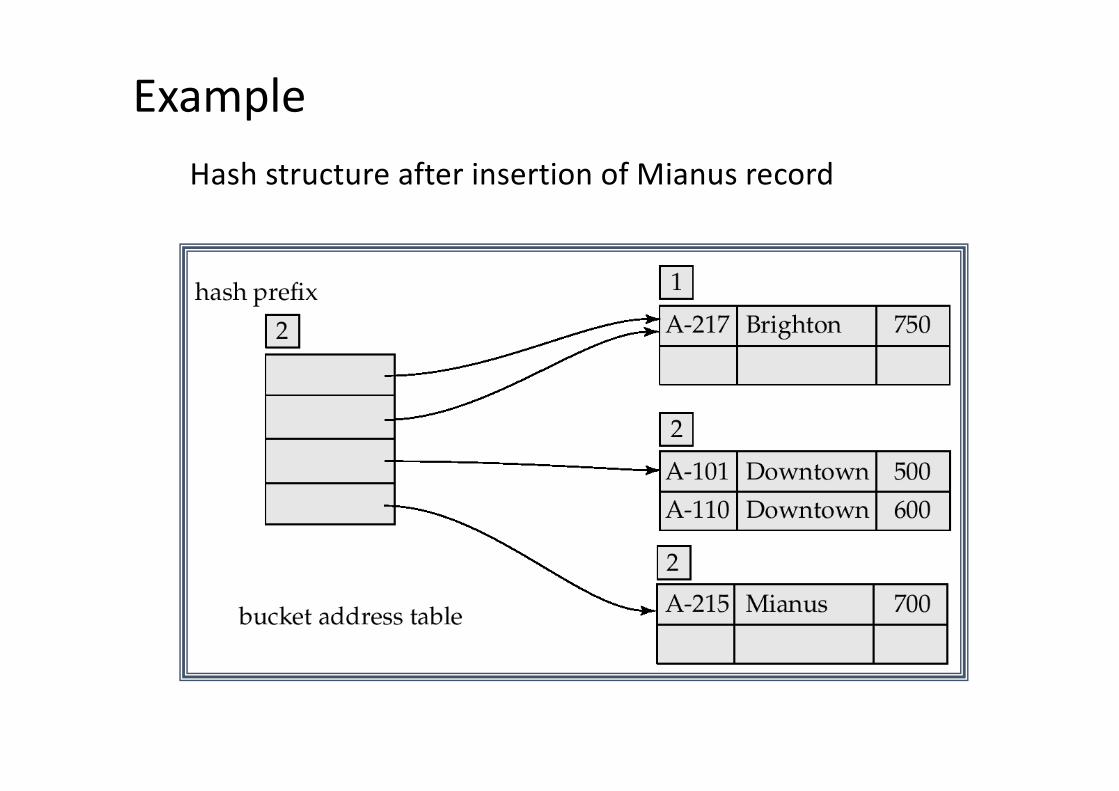
ExampleHash structure after insertion of Mianus record

Example
Hash structure after insertion of three Perryridge records
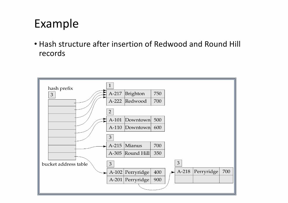
Example• Hash structure after insertion of Redwood and Round Hill
records

Comparison to Other Hashing Methods• Advantage: performance does not decrease as the database
size increases• Space is conserved by adding and removing as necessary
• Disadvantage: additional level of indirection for operations• Complex implementation
Ordered Indexing vs. Hashing• Hashing is less efficient if queries to the database include
ranges as opposed to specific values.• In cases where ranges are infrequent hashing provides faster
insertion, deletion, and lookup then ordered indexing.